Controllers and Controlled Systems

Technical Information

Part

1Fu

ndam

enta

ls

1Controllers and Controlled Systems

A A E A E A E A 1

2

3

y-t

A E

+

_

Generator Add PID PT1 PT1PT2 Time

PT1

Y

t

Part 1: Fundamentals

Part 2: Self-operated Regulators

Part 3: Control Valves

Part 4: Communication

Part 5: Building Automation

Part 6: Process Automation

Should you have any further questions or suggestions, pleasedo not hesitate to contact us:

SAMSON AG Phone (+49 69) 4 00 94 67V74 / Schulung Telefax (+49 69) 4 00 97 16Weismüllerstraße 3 E-Mail: [email protected] Frankfurt Internet: http://www.samson.de

Technical Information

Controller and Controlled Systems

Controller and Controlled Systems . . . . . . . . . . . . . . . . . . . 3

Introduction . . . . . . . . . . . . . . . . . . . . . . . . . . . . . 5

Controlled Systems . . . . . . . . . . . . . . . . . . . . . . . . . . 7

P controlled system . . . . . . . . . . . . . . . . . . . . . . . . . . . . . . . . . . . . 8

I controlled system . . . . . . . . . . . . . . . . . . . . . . . . . . . . . . . . . . . . . 9

Controlled system with dead time . . . . . . . . . . . . . . . . . . . . . . . . . 11

Controlled system with energy storing components . . . . . . . . . . . . . 12

Characterizing Controlled Systems . . . . . . . . . . . . . . . . . . 18

System response . . . . . . . . . . . . . . . . . . . . . . . . . . . . . . . . . . . . . 18

Proportional-action coefficient . . . . . . . . . . . . . . . . . . . . . . . . . . . 18

Nonlinear response. . . . . . . . . . . . . . . . . . . . . . . . . . . . . . . . . . . 19

Operating point (OP). . . . . . . . . . . . . . . . . . . . . . . . . . . . . . . . . . 20

Controllability of systems with self-regulation . . . . . . . . . . . . . . . . . 21

Controllers and Control Elements . . . . . . . . . . . . . . . . . . . 23

Classification . . . . . . . . . . . . . . . . . . . . . . . . . . . . . . . . . . . . . . . 23

Continuous and discontinuous controllers . . . . . . . . . . . . . . . . . . . 24

Auxiliary energy . . . . . . . . . . . . . . . . . . . . . . . . . . . . . . . . . . . . . 24

Determining the dynamic behavior . . . . . . . . . . . . . . . . . . . . . . . . 25

Continuous Controllers. . . . . . . . . . . . . . . . . . . . . . . . 27

Proportional controller (P controller) . . . . . . . . . . . . . . . . . . . . . . . 27

Proportional-action coefficient . . . . . . . . . . . . . . . . . . . . . . . . . . . 27

System deviation . . . . . . . . . . . . . . . . . . . . . . . . . . . . . . . . . . . . . 29

3

Part 1 ⋅ L102EN

SAM

SON

AG

⋅99/

10

CON

TEN

TS

Adjusting the operating point . . . . . . . . . . . . . . . . . . . . . . . . . . . . 30

Integral controller (I controller) . . . . . . . . . . . . . . . . . . . . . . . . . . . 35

Derivative controller (D controller) . . . . . . . . . . . . . . . . . . . . . . . . . 38

PI controllers . . . . . . . . . . . . . . . . . . . . . . . . . . . . . . . . . . . . . . . . 40

PID controller . . . . . . . . . . . . . . . . . . . . . . . . . . . . . . . . . . . . . . . 42

Discontinuous Controllers . . . . . . . . . . . . . . . . . . . . . . 45

Two-position controller . . . . . . . . . . . . . . . . . . . . . . . . . . . . . . . . 45

Two-position feedback controller . . . . . . . . . . . . . . . . . . . . . . . . . 47

Three-position controller and three-position stepping controller . . . . 48

Selecting a Controller . . . . . . . . . . . . . . . . . . . . . . . . 50

Selection criteria . . . . . . . . . . . . . . . . . . . . . . . . . . . . . . . . . . . . . 50

Adjusting the control parameters. . . . . . . . . . . . . . . . . . . . . . . . . . 51

Appendix A1: Additional Literature . . . . . . . . . . . . . . . . . . 54

4

Fundamentals ⋅ Controllers and Controlled Systems

SAM

SON

AG

⋅V74

/D

KE

CON

TEN

TS

Introduction

In everyday speech, the term �control� and its many variations is frequentlyused. We can control a situation, such as a policeman controlling the traffic,or a fireman bringing the fire under control. Or an argument may get out ofcontrol, or something might happen to us because of circumstances beyondour control. The term �control� obviously implies the restoration of a desirablestate which has been disturbed by external or internal influences.

Control processes exist in the most diverse areas. In nature, for instance, con-trol processes serve to protect plants and animals against varying environ-mental conditions. In economics, supply and demand control the price anddelivery time of a product. In any of these cases, disturbances may occur thatwould change the originally established state. It is the function of the controlsystem to recognize the disturbed state and correct it by the appropriate me-ans.

In a similar way as in nature and economics, many variables must be con-trolled in technology so that equipment and systems serve their intended pur-pose. With heating systems, for example, the room temperature must be keptconstant while external influences have a disturbing effect, such as fluctua-ting outside temperatures or the habits of the residents as to ventilation, etc.

In technology, the term �control� is not only applied to the control process, butalso to the controlled system. People, too, can participate in a closed loopcontrol process. According to DIN 19226, closed loop control is defined asfollows:

Closed loop control is a process whereby one variable, namely the variableto be controlled (controlled variable) is continuously moni-tored, comparedwith another variable, namely the reference variable and influenced in sucha manner as to bring about adaptation to the reference variable. The se-quence of action resulting in this way takes place in a closed loop in whichthe controlled variable continuously influences itself.

5

Part 1 ⋅ L102EN

SAM

SON

AG

⋅99/

10

control in

language use

control in

technology

Note: �Continuous� here also means a sufficiently frequent repetition of iden-tical individual processes of which the cyclic program sequence in digitalsampling controls is an example.

Being a little in the abstract, this definition is illustrated below with practicalexamples from control engineering applications. On the one hand, control-led systems and controllers will therefore be discussed as independent trans-fer elements and, on the other hand, their behavior in a closed control loopwill be shown and compared.

6


SAM

SON

AG

⋅V74

/D

KE

continuous or

sampling control

Controlled Systems

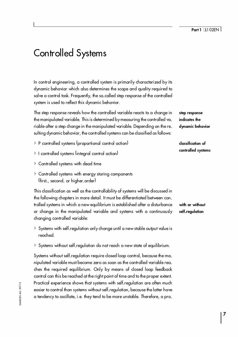
In control engineering, a controlled system is primarily characterized by itsdynamic behavior which also determines the scope and quality required tosolve a control task. Frequently, the so-called step response of the controlledsystem is used to reflect this dynamic behavior.

The step response reveals how the controlled variable reacts to a change inthe manipulated variable. This is determined by measuring the controlled va-riable after a step change in the manipulated variable. Depending on the re-sulting dynamic behavior, the controlled systems can be classified as follows:

4P controlled systems (proportional control action)

4 I controlled systems (integral control action)

4Controlled systems with dead time

4Controlled systems with energy storing components(first-, second- or higher-order)

This classification as well as the controllability of systems will be discussed inthe following chapters in more detail. It must be differentiated between con-trolled systems in which a new equilibrium is established after a disturbanceor change in the manipulated variable and systems with a continuouslychanging controlled variable:

4Systems with self-regulation only change until a new stable output value isreached.

4Systems without self-regulation do not reach a new state of equilibrium.

Systems without self-regulation require closed loop control, because the ma-nipulated variable must become zero as soon as the controlled variable rea-ches the required equilibrium. Only by means of closed loop feedbackcontrol can this be reached at the right point of time and to the proper extent.Practical experience shows that systems with self-regulation are often mucheasier to control than systems without self-regulation, because the latter havea tendency to oscillate, i.e. they tend to be more unstable. Therefore, a pro-

Part 1 ⋅ L102EN

SAM

SON

AG

⋅99/

10

7

step response

indicates the

dynamic behavior

classification of

controlled systems

with or without

self-regulation

perly adapted controller is more important in the case of systems withoutself-regulation.

P controlled system

In controlled systems with proportional action, the controlled variable xchanges proportional to the manipulated variable y. The controlled variablefollows the manipulated variable without any lag.

Since any energy transfer requires a finite amount of time, P control actionwithout any lag does not occur in practice. When the time lag between mani-pulated and controlled variable is so small, however, that it does not haveany effect on the system, this behavior is called proportional control action ofa system or a P controlled system.

4Example: Flow control

If the valve travel changes in the pressure control system illustrated in Fig. 1,a new flow rate q is reached (almost) instantaneously. Depending on the val-ve flow coefficient, the controlled variable changes proportional to the mani-pulated variable; the system has proportional control action.

Fig. 2 shows the block diagram symbol for proportional action and the dyna-mic behavior of a P controlled system after a step change in the input varia-

8


SAM

SON

AG

⋅V74

/D

KE

y

q = K * ys

q

y

Fig. 1: Proportional controlled system; reference variable: flow rate

P control action with-

out any lag is possible

in theory only

new equilibrium

without lag

ble. The characteristic curves clearly show that a proportional controlledsystem is a system with self-regulation, since a new equilibrium is reachedimmediately after the step change.

I controlled system

Integral controlled systems are systems without self-regulation: if the manipu-lated variable does not equal zero, the integral controlled system respondswith a continuous change � continuous increase or decrease � of the control-led variable. A new equilibrium is not reached.

4Example: Liquid level in a tank (Fig. 3)

In a tank with an outlet and equally high supply and discharge flow rates, aconstant liquid level is reached. If the supply or discharge flow rate changes,the liquid level will rise or fall. The level changes the quicker, the larger thedifference between supply and discharge flow.

This example shows that the use of integral control action is mostly limited inpractice. The controlled variable increases or decreases only until it reachesa system-related limit value: the tank will overflow or be discharged, maxi-mum or minimum system pressure is reached, etc.

9

Part 1 ⋅ L102EN

SAM

SON

AG

⋅99/

10

y ymax

y xt0 t

x xmax

t0 t

Fig. 2: Dynamic behavior of a P controlled system(y: control valve travel; x: flow rate in a pipeline)

block diagramm

systems without

self-regulation

marginal conditions

limit the I control action

Fig. 4 shows the dynamic behavior of an I controlled system after a stepchange in the input variable as well as the derived block diagram symbol forintegral control action. The integral-action time Tn serves as a measure forthe integral control action and represents the rise time of the controlledvariable. For the associated mathematical context, refer to the chapter�Controllers and Control Elements �.

10


SAM

SON

AG

⋅V74

/D

KE

H

L

Fig. 3: Integral controlled system; controlled variable: liquid level in a tank

y ymax

t0 tx

xmax

y x

t0

Ti

t

Fig. 4: Dynamic behavior of an I controlled system(y: valve travel; x: liquid level in a tank)

block diagramm

short integral-action

time causes high

rise time

Controlled system with dead time

In systems with dead time there is no dynamic response until a certainamount of time has elapsed. The time constant TL serves as a measure for thedead time or lag.

4Example: Adjustment of conveying quantity for conveyor belt (Fig. 5)

If the bulk material quantity fed to the conveyor belt is increased via slidegate, a change in the material quantity arriving at the discharge end of thebelt (sensor location) is only noticed after a certain time.

Pressure control in long gas pipes exhibits similar behavior. Since the medi-um is compressible, it takes some time until a change in pressure is noticeab-le at the end of the pipeline.

Often, several final control elements are the cause of dead times in a controlloop. These are created, e.g. through the switching times of contactors or theinternal clearance in gears.

Dead times are some of the most difficult factors to control in process controlsituations, since changes in the manipulated variable have a delaying effecton the controlled variable. Due to this delay, controlled systems with dead ti-mes often tend to oscillate. Oscillations always occur if controlled variableand manipulated variable periodically change toward each other, delayedby the dead time.

In many cases, dead times can be avoided or minimized by skillful planning(arrangement of the sensor and the control valve; if possible, by selectingshort pipelines; low heat capacities of the insulation media, etc. ).

11

Part 1 ⋅ L102EN

SAM

SON

AG

⋅99/

10

Fig. 5: Controlled system with dead time

delayed response

through lag

systems with dead

times tend to oscillate

Controlled system with energy storing components

Delays between changes in the manipulated and controlled variable are notonly created due to dead times. Any controlled system usually consists of se-veral components that are characterized by the capacity to store energy (e.g.heating system with heat storing pipes, jackets, insulation, etc.). Due to thesecomponents and their energetic state which changes only gradually, energyconsumption or discharge occurs time delayed. This also applies to all condi-tion changes of the controlled system, because these are originated in thetransfer or conversion of energy.

4Example: Room temperature control

A heating system is a controlled system with several energy storing compo-nents: boiler, water, radiator, room air, walls, etc.

When the energy supply to the boiler is changed or the radiator shut-off val-ve is operated in the heated room, the room temperature changes only gra-dually until the desired final value is reached.

It is characteristic of controlled systems with energy storing components thatthe final steady-state value is reached only after a finite time and that thespeed of response of process variable x changes during the transitional peri-

12


SAM

SON

AG

⋅V74

/D

KE

y ymax

t0 t

x xmax

y x

t0

TL

t

Fig. 6: Dynamic behavior of a controlled system with dead time(y: slide gate position; x: conveying quantity)

block diagram

delays caused by

storing components

od (Fig. 7). In principle, the speed of response slows down as it approachesits final value, until it asymptotically reaches its final value. While the outputvariable may suddenly change in systems with dead times, systems withenergy storing components can only change steadily.

The dynamic behavior of the system depends on those lags that produce thedecisive effect, thus, on the size of the existing storing components. Essential-ly, large components determine this factor so that smaller components fre-quently have no effect.

4Example: Room temperature control

The dynamic behavior of a room temperature control system is significantlyinfluenced by the burner capacity and the size of boiler, room and radiator.The dynamic behavior depends on the heating capacity of the heating pipesonly to a very small extent.

Controlled systems with energy storing components are classified accordingto the number of lags that produce an effect. For instance, a first-order sys-tem has one dynamic energy storing component, a second-order system hastwo energy storing components, etc. A system without any lags is also refer-red to as a �zero-order system� (see also P controlled system). A behavior re-sembling that of a zero-order system may occur in a liquid-filled pressuresystem without equalizing tanks.

13

Part 1 ⋅ L102EN

SAM

SON

AG

⋅99/

10

1

0,63

T1

x

t

Fig. 7: Exponential curves describe controlled systems with energy storingcomponents

exponential curves

characterize dynamic

behavior

classification of

systems with lags

one energy storingcomponent

more than one energystoring component

: time constant

� First-order system

A first-order system with only one dynamic energy storing component is illu-strated in Fig. 8: the temperature of a liquid in a tank equipped with inlet,outlet and agitator is adjusted via mixing valve. Due to the large tank volume,the temperature changes only gradually after the valve has been adjusted(step change).

The dynamic behavior of a first-order system is shown in Fig. 9. A measurefor the speed of response is the time constant T1. It represents the future time

14


SAM

SON

AG

⋅V74

/D

KE

Fig. 8: First-order controlled system; controlled variable: temperature

WW

KW T [°C]

H

y ymax

y xt0 t

x xmax

t0

T1

t

Fig. 9: Dynamic behavior of a first-order controlled system � PT1 element(y: valve position; x: temperature of liquid in tank)

block diagram

temperature control

via mixing valve

necessary for the controlled variable x (response curve) to reach 63% of itsfinal value after a step input has been introduced. The course of the functionis derived as follows:

Such delayed proportional behavior with a first-order lag is also referred toas PT1 behavior. The higher the time constant T1, the slower the change in thecontrolled variable and the larger the energy storing component causing thislag.

If the dynamic behavior of a system is only known as a response curve, T1

can be graphically determined with the help of the tangent shown in Fig. 9.

� Second-order and higher-order systems

If there are two or more energy storing components between themanipulated variable and the controlled variable, the controlled system isreferred to as second- or higher-order system (also called PT2, PT3 system,etc.). When two first-order systems are connected in series, the result is onesecond-order system, as shown in Fig. 10.

15

Part 1 ⋅ L102EN

SAM

SON

AG

⋅99/

10

( )x t etT= −

−1 1

Fig. 10: Second-order controlled system; controlled variable: temperature

H

T [°C]WW

KW

time constant defines

the dynamic behavior

n th order systems

exhibit PTn behavior

The dynamic behavior of such a system is reflected by the characteristic cur-ves shown in Fig. 11. The step response of the controlled variable shows aninflection point which is characteristic of higher-order systems (Figs. 11 and12): initially, the rate of change increases up to the inflection point and thencontinuously decreases (compare to behavior of first-order systems: Fig. 8).

Mathematically, the characteristic of a higher-order system is described bythe time constants T1, T2, etc. of the individual systems. The characteristiccurve for the step response is then derived as follows:

16


SAM

SON

AG

⋅V74

/D

KE

y ymax

y xt0 t

x xmax

t0 t

Fig. 11: Dynamic behavior of second- or higher-order controlled systems(y: valve position; x: medium temperature in the second tank)

y

xt

tTgTu

Fig. 12: Step response of a higher-order controlled system with the charac-teristic values Tu and Tg

block diagram

step response with

inflection point...

� and time constants

of the individual PT1

elements

tangent

inflectionpoint

For a simplified characterization of this behavior, the process lag Tu and theprocess reaction rate Tg are defined with the help of the inflection pointtangents (Fig. 12). Since process lag has the same effect as dead time, asystem is more difficult to control when Tu approaches the value of theprocess reaction rate Tg. The higher the system order, the less favorable doesthis relationship develop (Fig. 13).

The controllability improves, however, when the time constants T1, T2, etc.are as small as possible compared to the time required by the control loop forcorrective action. Highly different time constants (factor 10 or higher) alsosimplify the controller adjustment since it can then be focused on the highest,the time determining value. It is therefore on the part of the practitioner tocarefully consider these aspects already during the design phase of aprocess control system.

17

Part 1 ⋅ L102EN

SAM

SON

AG

⋅99/

10

( )x t e etT

tT= − −− −( ) ( )1 11 2

1x

t

Fig. 13: Dynamic behavior of higher-order controlled systems

first-order

fifth-order

fourth-order

third-order

second-order

time constants

characterize the

control response

Tu and Tg simplify

the evaluation

CharacterizingControlled Systems

System response

A complex controlled system can be described through the combined actionof several subsystems, each of which can be assigned with P, I, dead time orlag reaction. The system response is therefore a result of the combined actionof these individual elements (Fig. 14: Actuator with internal clearance in itsgears). In most cases, proportional or integral action occurs only after a cer-tain lag and/or dead time has elapsed.

The system-specific lags and/or dead times can also be so small that they donot have to be considered in the control process. In temperature controllers,for instance, the short time of opening the control valve can usually be ne-glected contrary to the much longer heating time.

Proportional-action coefficient

An important process variable in characterizing controlled systems withself-regulation is the factor KPS. This factor indicates the ratio of change in thecontrolled variable x to the corresponding change in the manipulated

18


SAM

SON

AG

⋅V74

/D

KE

y x

y x

Fig. 14: Dynamic behavior of an actuator with internal clearance in its gears(lagging integral response with dead time)

converter position (travel)internal clear-ance in gears

systems consist of

several subsystems

only time determining

elements are important

variable y under balanced, steady-state conditions:

To calculate KPS, the system must reach a new equilibrium after a step changein the manipulated variable ∆y. Since this requirement is only met by systemswith self-regulation, KPS is not defined for systems without self-regulation.

The factor KPS is frequently referred to as system gain. This term is not quitecorrect. If KPS is smaller than one, it does not have the effect of anamplification factor. Therefore, the proper term must be �proportional-actioncoefficient�. To ensure that the above relationship applies irrespective of thenature of the variables, input and output signals are normalized by dividingthem by their maximum values (100 % value).

Nonlinear response

In many practical applications, KPS is not constant over the complete range ofthe controlled variable, but changes depending on the correspondingoperating point. Such a response is termed nonlinear which is oftenencountered in temperature control systems.

19

Part 1 ⋅ L102EN

SAM

SON

AG

⋅99/

10

K xy

x xy yPS = =

−−

∆∆

2 1

2 1

w 20...100°Cx

Fig. 15: Steam-heated tank

dynamic behavior

depends on the

operating point

KPS: proportional-

action coefficient of the

system

4Example: Heating a steam-heated tank (Fig. 15)

A steam-heated water bath is a controlled system with self-regulation. Thewater bath and the tank material in which the pipeline is embedded are twolarge heat storing components which can be considered a second-ordercontrolled system. Since a body being heated will convey more and moreheat into the environment as the heating temperature increases, thecoefficient KPS changes with the water bath temperature (Fig. 16). Toincrease the temperature at high temperatures, comparatively more energymust be supplied than at low temperatures. Therefore, the following applies:

Operating point (OP)

If the reaction of nonlinear systems is analyzed with the help of stepresponses, a different dynamic behavior of the controlled variable can beobserved at each operating point. With the above illustration of water bathheating, entirely different values are obtained for KPS, Tu and Tg that dependon the operating temperature. This behavior is a disadvantage for thecontrolled system, because it leads to an operating point-dependent controlresponse of the system.

20


SAM

SON

AG

⋅V74

/D

KE

K C K CPS PS( ) ( )0 100° > °

T[°C]

∆T2

∆T1

∆P1 ∆P2 P[kW]

Fig. 16: Operating point-dependent behavior of the steam-heated tank

OP2

OP1

∆ ∆P P1 2=∆ Τ > ∆ Τ1 2

⇓

K OP K OPpS pS( ) ( )1 2>

heat dissipation

changes with the

temperature difference

nonlinearity makes

control more difficult

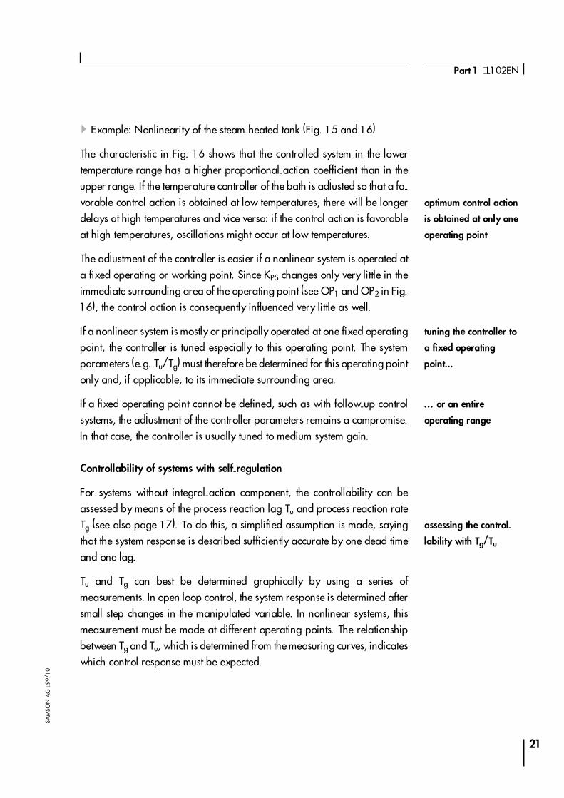
4Example: Nonlinearity of the steam-heated tank (Fig. 15 and 16)

The characteristic in Fig. 16 shows that the controlled system in the lowertemperature range has a higher proportional-action coefficient than in theupper range. If the temperature controller of the bath is adjusted so that a fa-vorable control action is obtained at low temperatures, there will be longerdelays at high temperatures and vice versa: if the control action is favorableat high temperatures, oscillations might occur at low temperatures.

The adjustment of the controller is easier if a nonlinear system is operated ata fixed operating or working point. Since KPS changes only very little in theimmediate surrounding area of the operating point (see OP1 and OP2 in Fig.16), the control action is consequently influenced very little as well.

If a nonlinear system is mostly or principally operated at one fixed operatingpoint, the controller is tuned especially to this operating point. The systemparameters (e.g. Tu/Tg) must therefore be determined for this operating pointonly and, if applicable, to its immediate surrounding area.

If a fixed operating point cannot be defined, such as with follow-up controlsystems, the adjustment of the controller parameters remains a compromise.In that case, the controller is usually tuned to medium system gain.

Controllability of systems with self-regulation

For systems without integral-action component, the controllability can beassessed by means of the process reaction lag Tu and process reaction rateTg (see also page 17). To do this, a simplified assumption is made, sayingthat the system response is described sufficiently accurate by one dead timeand one lag.

Tu and Tg can best be determined graphically by using a series ofmeasurements. In open loop control, the system response is determined aftersmall step changes in the manipulated variable. In nonlinear systems, thismeasurement must be made at different operating points. The relationshipbetween Tg and Tu, which is determined from the measuring curves, indicateswhich control response must be expected.

21

Part 1 ⋅ L102EN

SAM

SON

AG

⋅99/

10

optimum control action

is obtained at only one

operating point

tuning the controller to

a fixed operating

point...

� or an entire

operating range

assessing the control-

lability with Tg/Tu

4Example: Tu and Tg for controlled systems in process engineering

22


SAM

SON

AG

⋅V74

/D

KE

Controlledvariable

Type of controlledsystem

Tu Tg

Temperature Autoclaves Extruder 30 to 40 s1 to 6 min

10 to 20 min5 to 60 min

Pressure Oil-fired boiler 0 min 2.5 min

Flow rate Pipeline with gasPipeline with liquid

0 to 5 s0 s

0.2 s0 s

magnitude of

Tu and Tg

Ratio Tg/Tu System is ...

0 3< ≤TT

g

u

difficult to control;

3 10< <TT

g

u

only just controllable;

10 ≤TT

g

u

easy to control.

Controllers and Control Elements

A controller�s job is to influence the controlled system via control signal sothat the value of the controlled variable equals the value of the reference va-lue. Controllers consist of a reference and a control element (Fig. 17). The re-ference element calculates the error (e) from the difference betweenreference (w) and feedback variable (r), while the control element generatesthe manipulated variable (y) from the error:

Classification

Control elements can be designed in many different ways. For instance, themanipulated variable y can be generated

4mechanically or electrically,

4analog or digitally,

4with or without auxiliary energy

from the error e. Although these differences significantly influence the con-troller selection, they have (almost) no impact on the control response. Firstand foremost, the control response depends on the response of the manipu-lated variable. Therefore, controllers are classified according to their controlsignal response. Depending on the type of controller, the control signal caneither be continuous or discontinuous.

23

Part 1 ⋅ L102EN

SAM

SON

AG

⋅99/

10

e

x

w +

�

y

Fig. 17: Controller components

controller

controlelement

referenceelement x=r

functional principle

control signal response

⇔ control response

Continuous and discontinuous controllers

In continuous controllers, the manipulated variable can assume any valuewithin the controller output range. The characteristic of continuous controllersusually exhibits proportional (P), integral (I) or differential (D) action, or is asum of these individual elements (Fig. 18).

In discontinuous controllers, the manipulated variable y changes between di-screte values. Depending on how many different states the manipulated va-riable can assume, a distinction is made between two-position, three-position and multiposition controllers. Compared to continuous controllers,discontinuous controllers operate on very simple, switching final controllingelements. If the system contains energy storing components, the controlledvariable responds continuously, despite the step changes in the manipulatedvariable. If the corresponding time constants are large enough, good controlresults at small errors can even be reached with discontinuous controllersand simple control elements.

Auxiliary energy

Any controller and final controlling element requires energy to operate. Con-trollers externally supplied with pneumatic, electric or hydraulic energy areclassified as controllers with auxiliary energy. If no energy transfer mediumis available at the point of installation, self-operated regulators should be

24


SAM

SON

AG

⋅V74

/D

KE

Fig. 18: Classification of controllers

controllers

discontinuouscontrollers

continuoscontrollers

P controllerI controller

PD controller

PI controllerPID controller

two-position

multiposition

three-position

continuous...

...or discrete range of

the manipulated

variable

externally supplied

energy or energy deri-

ved from the system

used. They derive the energy they require to change the manipulated varia-ble from the controlled system. These cost-effective and rugged controllersare often used for pressure, differential pressure, flow and temperature con-trol. They can be used in applications where the point of measurement andthe point of change are not separated by great distances and where systemdeviations caused by energy withdrawal are acceptable.

Determining the dynamic behavior

As with the controlled systems, the following chapters will illustrate the dyna-mic behavior of individual controllers based on step responses (Fig. 19). Theresulting control response can be shown even more clearly in a closed con-trol loop.

25

Part 1 ⋅ L102EN

SAM

SON

AG

⋅99/

10

e PI

e y

y

Fig. 19: Step response of a controller

ew

w e y x

xyPI PT2

Fig. 20: Signal responses in a closed control loop

In a closed control loop, a step change in the reference variable first results ina step increase in the error signal e (Fig. 20). Due to the control action andthe feedback, the error signal will decrease in time. Finally, the controlled va-riable will reach a new steady state, provided that the control response is sta-ble (Fig. 20: Controlled variable x).

In order to be able to compare and analyze the response of different control-lers, each controller will be discussed in regard to its interaction with thesame �reference system�. This is a third-order system with the following para-meters:

Proportional-action coefficient: KP = 1

System parameters: T1 = 30 s; T2 = 15 s; T3 = 10 s .

The lag and the proportional-action of this system can be seen in Fig. 21. Itshows the step response, i.e. the response of the output variable (controlledvariable x) to a step change in the input variable (manipulated variable y).

26


SAM

SON

AG

⋅V74

/D

KE

Fig. 21: Step response the third-order reference system

comparison of control

responses based on

a ´reference system´

action flow in a closed

control loop

Continuous Controllers

Proportional controller (P controller)

The manipulated variable y of a P controller is proportional to the measurederror e. From this can be deducted that a P controller

4reacts to any deviation without lag and

4only generates a manipulated variable in case of system deviation.

The proportional pressure controller illustrated in Fig. 22 compares the forceFS of the set point spring with the force FM created in the elastic metal bellowsby the pressure p2. When the forces are off balance, the lever pivots aboutpoint D. This changes the position of the valve plug � and, hence, thepressure p2 to be controlled � until a new equilibrium of forces is restored.

� Proportional-action coefficient

The dynamic behavior of the P controller after a step change in the errorvariable is shown in Fig. 23. The amplitude of the manipulated variable y isdetermined by the error e and the proportional-action coefficient KP:

27

Part 1 ⋅ L102EN

SAM

SON

AG

⋅99/

10

manipulated variable

changes proportional

to error

p1 p2e

w

Kp

y x

Fig. 22: Design of a P controller (self-operated regulator)

metal bellow

D

set point spring

The term describes a linear equation whose gradient is determined by KP.Fig. 24 clearly shows that a high KP represents a strongly rising gradient, sothat even small system deviations can cause strong control actions.

Note: In place of the proportional-action coefficient KP, the old term�proportional band� is frequently used in literature which is represented bythe parameter XP[%]. The parameter is converted as follows:

28


SAM

SON

AG

⋅V74

/D

KE

e emax

e y

t1 t2t

y ymax

t1t2

t

Fig. 23: Dynamic behavior of a P controller(e: system devitation; y: manipulated variable)

y K eP= ⋅ with: K P as proportional-action coefficient

XKP

P

=100[%]

or KXP

P

=100[%]

block diagram

high KP causes

strong control action

proportional-action

coefficient or

proportional band

� System deviation

Controllers compensate for the effect of disturbance variables by generatinga corresponding manipulated variable acting in the opposite direction. SinceP controllers only generate a manipulated variable in case of system deviati-on (see definition by equation), a permanent change, termed �steady-stateerror�, cannot be completely balanced (Fig. 25).

Note: Stronger control action due to a high KP results in smaller systemdeviations. However, if KP values are too high, they increase the tendency ofthe control loop to oscillate.

29

Part 1 ⋅ L102EN

SAM

SON

AG

⋅99/

10

y y

y0Kp

ee

Fig. 24: Effect of KP and operating point adjustment

z

t

x

x0

t

e

Fig. 25: Steady-state error in control loops with P controllersx0: adjusted operating point of the controller

characteristic feature

of P controllers: steady-

state error

y0y0

� Adjusting the operating point

In the �ideal� control situation, i.e. with zero error, proportional-onlycontrollers do not generate control amplitudes (see above). This amplitude isrequired, however, if the controlled variable is to be kept at any level ofequilibrium in a system with self-regulation. In order to achieve this anyhow,P controllers require an option for adjusting the operating point. This optionis provided by adding a variable offset y0 to the manipulated variable of the

P controller:

This way, any control amplitude y0 can be generated, even with zero error.In mathematical terms, this measure corresponds to a parallel displacementof the operating characteristic over the entire operating range (see Fig. 24).

Note: Selecting an operating point � y0 nonzero � only makes sense forsystems with self-regulation. A system without self-regulation will only reachsteady state when the manipulated variable equals zero (example:motor-driven actuator).

4Example: Operating point and system deviation in pressure reducing val-ves

In a pressure control system (Fig. 26), p2 lies within the range of 0 to 20 bar,the operating point (pOP, qOp) is pOp = 8 bar.

If the proportional-action coefficient is set to KP = 10, the valve passesthrough the entire travel range with a 10 percent error. If the spring is notpreloaded (y0 = 0), the pressure reducing valve is fully open at 0 bar (H100)and fully closed at 2 bar (H0). The operating point (pOP, qOP) is not reached;significant system deviation will occur.

With the help of the operating point adjustment the spring can be preloadedin such a manner that the valve releases the cross-sectional area which isexactly equivalent to the operating point at p2 = 8 bar => zero systemdeviation.

30


SAM

SON

AG

⋅V74

/D

KE

y K e yP= ⋅ + 0 y0 : manipulated variable at operating point

selection of the

control amplitude

at steady state

operating point

adjustment by

preloading the spring

For instance, this would allow the following assignment (Fig. 26):

There is a maximum system deviation of ≤ 0.5 bar over the entire valve travelrange. If this is not tolerable, KP must be increased: a KP of 50 reduces thesystem deviation to ≤ 0.2 bar (20 bar/50 = 0.4 bar). However, KP cannot beincreased infinitely. If the response in the controller is too strong, thecontrolled variable will overshoot, so that the travel adjustment must besubsequently reversed for counteraction: the system becomes instable.

31

Part 1 ⋅ L102EN

SAM

SON

AG

⋅99/

10

20

10

8

6

2

qAP

p1 p2

KP = 50Kp = 10

q0 qmax

HAPH0 H100

Fig. 26: Functional principle and characteristics of a pressure reducing valve

9,0 bar: valve closed H0

8,0 bar: valve in mid-position (qOP) HOP

7,0 bar: valve fully open H100

high KP reduces system

deviation and increa-

ses the tendency to

oscillate

� Example: Proportional level control

The water in a tank (Fig. 27) is to be kept at a constant level, even if the outputflow rate of the water is varied via the drain valve (VA).

The illustrated controlling system is at steady state when the supplied as wellas the drained water flow rates are equally large the liquid level remainsconstant.

If the drain valve (VA) is opened a little further, the water level will start to fall.The float (SW) in the tank will descend together with the water level. This willcause the rigid lever connected to the float to open the inlet valve (VE). The in-creasing flow finally prevents the water level from dropping still lower so thatthe system reaches a new equilibrium level.

By displacing the pivot of the lever upward or downward, a different statio-nary water level can be adjusted. If the individual components are sized pro-perly, this type of control process will prevent the tank from discharging oroverflowing.

The above example shows the typical characteristics of proportional controlaction:

32


SAM

SON

AG

⋅V74

/D

KE

SW

L

W

Kp

VE

VA

Fig. 27: Level control with a P controller (self-operated regulator)

level control:

principle of operation

4 In case of disturbances, steady-state error is always sustained: when theoutlet flow rate permanently changes, it is urgently required for the liquidlevel to deviate from the originally adjusted set point to permanently chan-ge the position of the inlet valve (VE) as well.

4The system deviation decreases at high gain (high proportional action co-efficient), but also increases the risk of oscillation for the controlled varia-ble. If the pivot of the lever is displaced towards the float, the controllersensitivity increases. Due to this amplified controlling effect, the supplyflow changes more strongly when the level varies; too strong an amplifica-tion might lead to sustained variations in the water level (oscillation).

Note: The illustrated level control system uses a self-operated regulator. Thecontrol energy derived from the system is characteristic of this controller type:the weight of the float and the positioning forces are compensated for by thebuoyancy of the float caused by its water displacement.

� Control response (based on the example of the PT3 system)

Control of a PT3 system (KP = 1; T1 = 30 s; T2 = 15 s; T3 = 10 s) with a Pcontroller results in the control response shown in Fig. 28. As previouslymentioned, the system�s tendency for oscillation increases with increasing KP,while the steady-state error is simultaneously reduced.

33

Part 1 ⋅ L102EN

SAM

SON

AG

⋅99/

10

Fig. 28: Control response of the P controller based on a PT3 system

limit values in

adjusting KP

self-operated

regulators for simple

control tasks

steady-state error

P controllers exhibit the following advantages:

4Fast response to changes in the control process due to immediate correcti-ve action when an error occurs.

4Very stable control process, provided that KP is properly selected.

P controllers exhibit the following disadvantages:

4Steady-state error when disturbances occur, since only system deviationcauses a change in the manipulated variable.

P controller applications:P controllers are suited to noncritical control applications which can toleratesteady-state error in the event of disturbances: e.g. pressure, flow rate, leveland temperature control. P control action provides rapid response, althoughits dynamic properties can still be improved through additional control com-ponents, as described on page 38 ff.

34


SAM

SON

AG

⋅V74

/D

KE

P controllers: fast and

stable with steady-

state error

Integral controller (I controller)

Integral control action is used to fully correct system deviations at anyoperating point. As long as the error is nonzero, the integral action willcause the value of the manipulated variable to change. Only when referencevariable and controlled variable are equally large � at the latest, though,when the manipulated variable reaches its system specific limit value (Umax,pmax, etc.) � is the control process balanced. Mathematics expresses integralaction as follows: the value of the manipulated variable is changedproportional to the integral of the error e.

How rapidly the manipulated variable increases/decreases depends on theerror and the integral time Tn (reciprocal of integral-action coefficient Ki). Ifthe controller has a short integral time, the control signal increases morerapidly as for controllers with long integral time (small integral-actioncoefficient).

Note: The higher the integral action coefficient Ki, the greater the integralaction of an I controller, or it is the lower, the higher the integral time value Tn.

35

Part 1 ⋅ L102EN

SAM

SON

AG

⋅99/

10

y K e dti= ∫ with: KTi

n

=1

no error in

steady state

p1 p2

xy

Fig. 29: I pressure controller

metalbellow

set point spring

high Tn ⇒ slow

control action

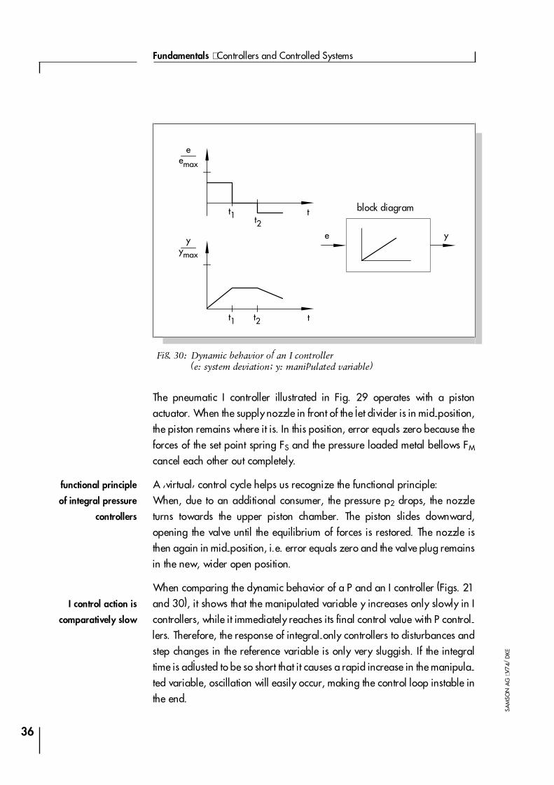
The pneumatic I controller illustrated in Fig. 29 operates with a pistonactuator. When the supply nozzle in front of the jet divider is in mid-position,the piston remains where it is. In this position, error equals zero because theforces of the set point spring FS and the pressure loaded metal bellows FM

cancel each other out completely.

A �virtual� control cycle helps us recognize the functional principle:When, due to an additional consumer, the pressure p2 drops, the nozzleturns towards the upper piston chamber. The piston slides downward,opening the valve until the equilibrium of forces is restored. The nozzle isthen again in mid-position, i.e. error equals zero and the valve plug remainsin the new, wider open position.

When comparing the dynamic behavior of a P and an I controller (Figs. 21and 30), it shows that the manipulated variable y increases only slowly in Icontrollers, while it immediately reaches its final control value with P control-lers. Therefore, the response of integral-only controllers to disturbances andstep changes in the reference variable is only very sluggish. If the integraltime is adjusted to be so short that it causes a rapid increase in the manipula-ted variable, oscillation will easily occur, making the control loop instable inthe end.

36


SAM

SON

AG

⋅V74

/D

KE

e emax

e y

t1 t2t

y ymax

t1 t2 t

Fig. 30: Dynamic behavior of an I controller(e: system deviation; y: manipulated variable)

block diagram

functional principle

of integral pressure

controllers

I control action is

comparatively slow


Fig. 31 shows how the PT3 system (KP = 1; T1 = 30 s; T2 = 15 s; T3 = 10 s) iscontrolled with an I controller. Contrary to Fig. 28 which showsproportional-action control, the time scale was doubled in this illustration. Itclearly shows that the I controller�s response is considerably slower, while thecontrol dynamics decreases with increasing Tn. A positive feature is thenonexistent error at steady state.

Note: Adjusting an operating point would not make any sense for I control-lers, since the integral action component would correct any set-point deviati-on. The change in the manipulated variable until error has been eliminated isequivalent to an �automated� operating point adjustment: the manipulatedvariable of the I controller at steady state (e=0) remains at a value whichwould have to be entered for P controllers via the operating point adjuster.

I controllers exhibit the following advantages:

4No error at steady state

I controllers exhibit the following disadvantages:

4Sluggish response at high Tn

4At small Tn, the control loop tends to oscillate/may become instable

37

Part 1 ⋅ L102EN

SAM

SON

AG

⋅99/

10

Fig. 31: Control response of the I controller with PT3 system(double time scale)

no steady-state error...

� by self-adaption to

the operating point

Derivative controller (D controller)

D controllers generate the manipulated variable from the rate of change ofthe error and not � as P controllers � from their amplitude. Therefore, they re-act much faster than P controllers: even if the error is small, derivative con-trollers generate � by anticipation, so to speak � large control amplitudes assoon as a change in amplitude occurs. A steady-state error signal, however,is not recognized by D controllers, because regardless of how big the error,its rate of change is zero. Therefore, derivative-only controllers are rarelyused in practice. They are usually found in combination with other controlelements, mostly in combination with proportional control.

In PD controllers (Fig. 32) with proportional-plus-derivative control action,the manipulated variable results from the addition of the individual P and Dcontrol elements:

The factor TV is the rate time, KD is the derivative-action coefficient. Bothvariables are a measure for the influence of the D component: high valuesmean strong control action.

As with the P controller, the summand y0 stands for the operating pointadjustment, i.e. the preselected value of the manipulated variable which isissued by the controller in steady state when e = 0.

38


SAM

SON

AG

⋅V74

/D

KE

y K e Kdedt

yP D= ⋅ + + 0 with: K K TD p v= ⋅

PD

P

D

e y e y=

Fig. 32: Elements of a PD controller

rapid response

to any change

combined P and

D controllers

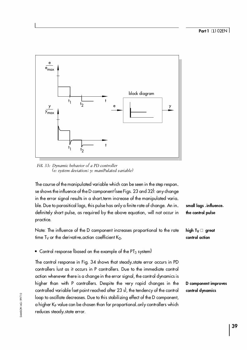
The course of the manipulated variable which can be seen in the step respon-se shows the influence of the D component (see Figs. 23 and 32): any changein the error signal results in a short-term increase of the manipulated varia-ble. Due to parasitical lags, this pulse has only a finite rate of change. An in-definitely short pulse, as required by the above equation, will not occur inpractice.

Note: The influence of the D component increases proportional to the ratetime TV or the derivative-action coefficient KD.


The control response in Fig. 34 shows that steady-state error occurs in PDcontrollers just as it occurs in P controllers. Due to the immediate controlaction whenever there is a change in the error signal, the control dynamics ishigher than with P controllers. Despite the very rapid changes in thecontrolled variable (set point reached after 23 s), the tendency of the controlloop to oscillate decreases. Due to this stabilizing effect of the D component,a higher KP value can be chosen than for proportional-only controllers whichreduces steady-state error.

39

Part 1 ⋅ L102EN

SAM

SON

AG

⋅99/

10

e emax

e yt1 t2

ty

ymax

t1 t2t

Fig. 33: Dynamic behavior of a PD controller(e: system deviation; y: manipulated variable)

block diagram

small lags ´influence´

the control pulse

high TV ⇒ great

control action

D component improves

control dynamics

PD controllers are employed in all applications where P controllers are notsufficient. This usually applies to controlled systems with greater lags, inwhich stronger oscillation of the controlled variable � caused by a high KP

value � must be prevented.

PI controllers

PI controllers are often employed in practice. In this combination, one P andone I controller are connected in parallel (Fig. 35). If properly designed, theycombine the advantages of both controller types (stability and rapidity; nosteady-state error), so that their disadvantages are compensated for at thesame time.

40


SAM

SON

AG

⋅V74

/D

KE

Fig. 34:Control response of the PD controller with PT3 system

PI

P

I

e y e y=

Fig. 35: Elements of a PI controller

suited to many

control tasks

The manipulated variable of PI controllers is calculated as follows:

The dynamic behavior is marked by the proportional-action coefficient KP

and the reset time Tn. Due to the proportional component, the manipulatedvariable immediately reacts to any error signal e, while the integralcomponent starts gaining influence only after some time. Tn represents thetime that elapses until the I component generates the same control amplitudethat is generated by the P component (KP) from the start (Fig. 36). As with Icontrollers, the reset time Tn must be reduced if the integral-action componentis to be amplified.


As expected, PI control of the PT3 system (Fig. 37) exhibits the positiveproperties of P as well as of I controllers. After rapid corrective action, thecontrolled variable does not show steady-state error. Depending on how

41

Part 1 ⋅ L102EN

SAM

SON

AG

⋅99/

10

e emax

e y

t1 t2t

y ymax

t1 t2 t

Tn

Fig. 36: Dynamic behavior of a PI controller(e: system deviation; y: manipulated variable)

y K e K e dtp i= ⋅ + ∫ with: KKTi

p

n

=

block diagram

division of tasks bet-

ween P and I control-

lers: fast and accurate

high the KP and Tn values are, oscillation of the controlled variable can bereduced, however, at the expense of control dynamics.

PI controller applications:Control loops allowing no steady-state error.Examples: pressure, temperature, ratio control, etc.

PID controller

If a D component is added to PI controllers, the result is an extremely versatilePID controller (Fig. 38). As with PD controllers, the added D component � ifproperly tuned � causes the controlled variable to reach its set point morequickly, thus reaching steady state more rapidly.

42


SAM

SON

AG

⋅V74

/D

KE

Fig. 37: Control response of the PI controller with PT3 system

=PID

P

I

D

e y e y

Fig. 38: Elements of a PID controller

PI controller with

improved control

dynamics

variable controller

design

In addition to the manipulated variable generated by the PI component (Fig.36), the D component increases the control action with any change in error(Fig. 39). Thus, the manipulated variable y results from the addition of thedifferently weighted P, I and D components and their associated coefficients:


The control response of PID controllers is favorable in systems with largeenergy storing components (higher-order controlled systems) that requirecontrol action as fast as possible and without steady-state error.

Compared to the previously discussed controllers, the PID controller thereforeexhibits the most sophisticated control response (Fig. 40) in the referencesystem example. The controlled variable reaches its set point rapidly,stabilizes within short, and oscillates only slightly about the set point. Thethree control parameters KP, Tn and TV provide an immense versatility in

43

Part 1 ⋅ L102EN

SAM

SON

AG

⋅99/

10

e emax

e y

t1 t2t

y ymax

t1 t2 t

Fig. 39: Dynamic behavior of a PID controller(e: system deviation; y: manipulated variable)

y K e K e dt K dedtp i D= ⋅ + +∫ with K

KT

K K TiP

nD P V= = ⋅;

block diagram

three control modes

provide high flexibility..

accurate and highly

dynamic control

adjusting the control response with respect to amplitude and controldynamics. It is therefore especially important that the controller be designedand tuned with care as well as be adapted to the system as good as possible(see chapter: Selecting a Controller).

PID controller applications:Control loops with second- or higher-order systems that require rapid stabili-zation and do not allow steady-state error.

44


SAM

SON

AG

⋅V74

/D

KE

Fig. 40: Control response of the PID controller with PT3 system

� and require careful

tuning adjustments

Discontinuous Controllers

Discontinuous controllers are also frequently called switching controllers. Themanipulated variable in discontinuous controllers assumes only a few discre-te values, so that energy or mass supply to the system can be changed only indiscrete steps.

Two-position controller

The simplest version of a discontinuous controller is the two-positioncontroller which, as the name indicates, has only two different output states,for instance 0 and ymax according to Fig. 41.

A typical application is temperature control by means of a bimetallic strip(e.g. irons). The bimetal serves as both measuring and switching element. Itconsists of two metal strips that are welded together, with each strip expan-ding differently when heated (Fig. 42).

If contact is made � bimetal and set point adjuster are touching � a currentsupplies the hot plate with electricity. If the bimetallic strip is installed near thehot plate, it heats up as well. When heated up, the bottom material expandsmore than the top material. This causes the strip to bend upward as the heatincreases, and it finally interrupts the energy supply to the heating coil. If thetemperature of the bimetal decreases, the electrical contact is made again,starting a new heating phase.

45

Part 1 ⋅ L102EN

SAM

SON

AG

⋅99/

10

y

ymax ymaxx

y

w x w xx x

Fig. 41: Switching charakteristic of the two-position controller(without and with differential gap xdg)

wxbot xtop

cyclic on/off switching

only definite number

of switching states

example: temperature

control via bimetal

xdg

To increase the service life of the contacts, as shown in Fig. 42, a differentialgap xdg can be created by using an iron plate and a permanent magnet. Theconditions for on/off switching are not identical anymore (xbot and xtop

according to Fig. 41), so that the switching frequency is reduced and sparkgeneration is largely prevented.

46


SAM

SON

AG

⋅V74

/D

KE

Ts

x

x

xmax

x

yt

t

Fig. 42: Control cycle of a two-position controller with differential gap andfirst-order controlled system

top

botxdg

differential gap

reduces switching

frequency

NS

Fe

~_ Q

.

I

Fig. 43: Temperature control via bimetallic switch

thermal convection

magnet

The typical behavior of manipulated and controlled variable as a function oftime in a two-position controller can be seen in Fig. 43. The dotted characte-ristic shows that at higher set points the temperature increase takes longerthan the cooling process. In this example we assume that the energy inflow(here: heating capacity) is sufficient to reach double the value of the selectedset point. The capacity reserve of 100% chosen here has the effect thaton/off switching periods are identical.

The temperature curve shown in Fig. 43 identifies a first-order controlledsystem. In higher-order controlled systems, the controlled variable wouldfollow the manipulated variable only sluggishly due to the lag. This causesthe controlled variable to leave the tolerance band formed by the switchingpoints xtop and xbot (Fig. 44). This effect must be taken into considerationwhen tuning the controller by applying the measures described below.

Two-position feedback controller

Should the displacement of the controlled variable as shown in Fig. 44 not betolerable, the differential gap can be reduced. This causes the switching fre-

47

Part 1 ⋅ L102EN

SAM

SON

AG

⋅99/

10

x

x∆xx

y t

t

Fig. 44: Control cycle of a two-position controller with differential gap andhigher-order controlled system

xtop

xbot

additional system

deviation due to lag

quency to increase, thus exposing the contacts to more wear. Therefore, atwo-position feedback controller is often better suited to controlling sluggishhigher-order systems.

In a two-position feedback temperature controller, an additional internalheating coil heats up the bimetallic strip when the controller is switched on,thus causing a premature interruption of energy supply. If properly adjusted,this measure results in a less irregular amplitude of the controlled variable atan acceptable switching frequency.

Three-position controller and three-position stepping controller

Three-position controllers can assume three different switching states. In atemperature control system, these states are not only �off� and �heating� as ina two-position controller, but also �cooling�. Therefore, a three-position con-troller fulfills the function of two coupled two-position controllers that switchat different states; this can also be seen in the characteristic of a three- positi-on controller with differential gap (Fig. 45).

In the field of control valve technology, three-position controllers are fre-quently used in combination with electric actuators. The three states of �coun-terclockwise� (e.g. opening), �clockwise� (e.g. closing) and �off� can be usedto adjust any valve position via relay and actuator motor (Fig. 46). Using adiscontinuous controller with integrated actuator (e.g. actuator motor) and

48


SAM

SON

AG

⋅V74

/D

KE

xymax

–ymax

x x

w

A B C

Fig. 45: Characteristic of a three-position controller with differential gap xdgand dead band xd

three-position control-

led actuator motors

quasi-continuous

control

xdg xdgxd

feedback control

improves the

control quality

applying suitable control signals, the result is a quasi-continuous P, PI or PIDcontrol response. Such three-position stepping controllers are frequentlyused in applications where pneumatic or hydraulic auxiliary energy is notavailable, but electric auxiliary energy.

When properly adapted to the system, the control response of a three-position stepping controller can barely be differentiated from that of acontinuous controller. Its control response may even be more favorable, forinstance, when the noise of a controlled variable caused by disturbances iswithin the dead band xd.

49

Part 1 ⋅ L102EN

SAM

SON

AG

⋅99/

10

e yyR

yR

y

t

t

Fig. 46: Control signal of a quasi-continuous controller(three-position controller with actuator motor)

Selecting a Controller

Selection criteria

To solve a control task it is required that

4 the controlled system be analyzed and

4a suitable controller be selected and designed.

The most important properties of the widely used P, PD, I, PI and PID controlelements are listed in the following table:

Which controller to select depends on the following factors:

4 Is the system based on integral or proportional control action (with or wit-hout self-regulation)?

4How great is the process lag (time constants and/or dead times)?

4How fast must errors be corrected?

4 Is steady-state error acceptable?

According to the previous chapters (see also above table), controllers andsystems can be assigned to each other as follows:

P controllers are employed in easy-to-control systems where steady-state er-ror is acceptable. A stable and dynamic control response is reached at mini-mum effort.

50


SAM

SON

AG

⋅V74

/D

KE

Control

element

Offset Operating point

adjustment

Speed of

response

P yes recommended high

PD yes recommended very high

I no N/A low

PI no N/A high

PID no N/A very high

what to consider when

selecting a controller

P controllers

It makes sense to employ PD controllers in systems with great lag where offsetis tolerable. The D component increases the speed of response so that controldynamics improve compared to P controllers.

I controllers are suitable for use in applications with low requirements as tothe control dynamics and where the system does not exhibit great lag. It is anadvantage that errors are completely eliminated.

PI controllers combine the advantages of both P and I controllers. This type ofcontroller produces a dynamic control response without exhibiting stea-dy-state error. Most control tasks can be solved with this type of controller.However, if it is required that the speed of response be as high as possible re-gardless of the great lag, a PID controller will be the proper choice.

PID controllers are suitable for systems with great lag that must be eliminatedas quick as possible. Compared to the PI controller, the added D componentresults in better control dynamics. Compared to the PD controller, the added Icomponent prevents error in steady state.

The selection of an appropriate controller significantly depends on the corre-sponding system parameters. Therefore, the above mentioned applicationsshould only be considered a general guideline; the suitability of a certaintype of controller must be thoroughly investigated to accommodate the pro-cess it controls.

Adjusting the control parameters

For a satisfactory control result, the selection of a suitable controller is animportant aspect. It is even more important that the control parameters KP, Tn

and TV be appropriately adjusted to the system response. Mostly, theadjustment of the controller parameters remains a compromise between avery stable, but also very slow control loop and a very dynamic, but irregularcontrol response which may easily result in oscillation, making the controlloop instable in the end.

For nonlinear systems that should always work in the same operating point,e.g. fixed set point control, the controller parameters must be adapted to thesystem response at this particular operating point. If a fixed operating pointcannot be defined, such as with follow-up control systems, the controller must

51

Part 1 ⋅ L102EN

SAM

SON

AG

⋅99/

10

PD controllers

I controllers

PI controllers

PID controllers

objectives in tuning

controllers

adaptation to operating

point or range

be adjusted to ensure a sufficiently rapid and stable control result within theentire operating range.

In practice, controllers are usually tuned on the basis of values gained by ex-perience. Should these not be available, however, the system response mustbe analyzed in detail, followed by the application of several theoretical orpractical tuning approaches in order to determine the proper control para-meters.

One approach is a method first proposed by Ziegler and Nichols, theso-called ultimate method. It provides simple tuning that can be applied inmany cases. This method, however, can only be applied to controlled sys-tems that allow sustained oscillation of the controlled variable. For this me-thod, proceed as follows:

4At the controller, set KP and TV to the lowest value and Tn to the highestvalue (smallest possible influence of the controller).

4Adjust the controlled system manually to the desired operating point (startup control loop).

4Set the manipulated variable of the controller to the manually adjusted va-lue and switch to automatic operating mode.

4Continue to increase KP (decrease XP) until the controlled variableencounters harmonic oscillation. If possible, small step changes in the setpoint should be made during the KP adjustment to cause the control loop tooscillate.

4Take down the adjusted KP value as critical proportional-action coefficientKP,crit.

52


SAM

SON

AG

⋅V74

/D

KE

KP Tn Tv

P 0 50, , .⋅K p crit - -

PI 0 45, , .⋅K p crit 0 85, .⋅Tcrit -

PID 0 59, , .⋅K P crit 0 50, .⋅Tcrit 0 12, .⋅Tcrit

Fig. 47: Adjustment values of control parameters acc. to Ziegler/Nichols: atK P crit, ., the controlled variable oscillates periodically with Tcrit.

ultimate tuning method

by Ziegler and Nichols

4Determine the time span for one full oscillation amplitude as Tcrit, ifnecessary by taking the time of several oscillations and calculating theiraverage.

4Multiply the values of KP,crit and Tcrit by the values according to the table inFig. 47 and enter the determined values for KP, Tn and TV at the controller.

4 If required, readjust KP and Tn until the control loop shows satisfactorydynamic behavior.

Part 1 ⋅ L102EN

SAM

SON

AG

⋅99/

10

53

Appendix A1:Additional Literature

[1] Terminology and Symbols in Control EngineeringTechnical Information L101EN; SAMSON AG

[2] Anderson, Norman A.: Instrumentation for Process Measurementand Control. Radnor, PA: Chilton Book Company

[3] Murrill, Paul W.: Fundamentals of Process Control Theory. ResearchTriangle Park, N.C.: Instrument Society of America, 1981

[4] DIN 19226 Part 1 to 6 �Leittechnik: Regelungstechnik undSteuerungstechnik� (Control Technology). Berlin: Beuth Verlag

[5] �International Electrotechnical Vocabulary�, Chapter 351:Automatic control. IEC Publication 50.

54


SAM

SON

AG

⋅V74

/D

KE

APP

ENDI

X

Figures

Fig. 1: Proportional controlled system; reference variable: flow rate . . 8

Fig. 2: Dynamic behavior of a P controlled system . . . . . . . . . . . 9

Fig. 3: Integral controlled system; controlled variable: liquid level . . . 10

Fig. 4: Dynamic behavior of an I controlled system . . . . . . . . . . 10

Fig. 5: Controlled system with dead time. . . . . . . . . . . . . . . 11

Fig. 6: Dynamic behavior of a controlled system with dead time . . . 12

Fig. 7: Exponential curves describe controlled systems . . . . . . . . 13

Fig. 8: First-order controlled system . . . . . . . . . . . . . . . . . 14

Fig. 9: Dynamic behavior of a first-order controlled system . . . . . . 14

Fig. 10: Second-order controlled system . . . . . . . . . . . . . . . 15

Fig. 11: Dynamic behavior of second- or higher-order controlled systems 16

Fig. 12: Step response of a higher-order controlled system . . . . . . . 16

Fig. 13: Dynamic behavior of higher-order controlled systems . . . . . 17

Fig. 14: Dynamic behavior of an actuator . . . . . . . . . . . . . . 18

Fig. 15: Steam-heated tank . . . . . . . . . . . . . . . . . . . . . 19

Fig. 16: Operating point-dependent behavior of the steam-heated tank. 20

Fig. 17: Controller components . . . . . . . . . . . . . . . . . . . 23

Fig. 18: Classification of controllers . . . . . . . . . . . . . . . . . 24

Fig. 19: Step response of a controller . . . . . . . . . . . . . . . . . 25

Fig. 20: Signal responses in a closed control loop . . . . . . . . . . . 25

Fig. 21: Step response the third-order reference system . . . . . . . . 26

Fig. 22: Design of a P controller (self-operated regulator) . . . . . . . 27

55

Part 1 ⋅ L102EN

SAM

SON

AG

⋅99/

10

FIG

URE

S

Fig. 23: Dynamic behavior of a P controller . . . . . . . . . . . . . . 28

Fig. 24: Effect of KP and operating point adjustment . . . . . . . . . . 29

Fig. 25: Steady-state error in control loops with P controllers . . . . . . 29

Fig. 26: Functional principle of a pressure reducing valve . . . . . . . 31

Fig. 27: Level control with a P controller (self-operated regulator) . . . . 32

Fig. 28: Control response of the P controller based on a PT3 system . . . 33

Fig. 29: I pressure controller . . . . . . . . . . . . . . . . . . . . . 35

Fig. 30: Dynamic behavior of an I controller . . . . . . . . . . . . . 36

Fig. 31: Control response of the I controller with PT3 system . . . . . . 37

Fig. 32: Elements of a PD controller. . . . . . . . . . . . . . . . . . 38

Fig. 33: Dynamic behavior of a PD controller . . . . . . . . . . . . . 39

Fig. 34: Control response of the PD controller with PT3 system . . . . . 40

Fig. 35: Elements of a PI controller . . . . . . . . . . . . . . . . . . 40

Fig. 36: Dynamic behavior of a PI controller . . . . . . . . . . . . . 41

Fig. 37: Control response of the PI controller with PT3 system . . . . . . 42

Fig. 38: Elements of a PID controller . . . . . . . . . . . . . . . . . 42

Fig. 39: Dynamic behavior of a PID controller . . . . . . . . . . . . . 43

Fig. 40: Control response of the PID controller with PT3 system . . . . . 44

Fig. 41: Switching charakteristic of the two-position controller . . . . . 45

Fig. 42: Control cycle of a two-position controller (first-order) . . . . . 46

Fig. 43: Temperature control via bimetallic switch . . . . . . . . . . . 46

Fig. 44: Control cycle of a two-position controller (higher-order) . . . . 47

Fig. 45: Characteristic of a three-position controller . . . . . . . . . . 48

Fig. 46: Control signal of a quasi-continuous controller . . . . . . . . 49

Fig. 47: Adjustment values of control parameters acc. to Ziegler/Nichols 52

56


SAM

SON

AG

⋅V74

/D

KE

FIG

URE

S

57

Part 1 ⋅ L102EN

SAM

SON

AG

⋅99/

10

NO

TES

58


SAM

SON

AG

⋅V74

/D

KE

NO

TES

SAMSON right on quality course

ISO 9001Our quality assurance system,

approved by BVQi, guarantees a high

quality of products and services.

SAMSON AG ⋅ MESS- UND REGELTECHNIK ⋅ Weismüllerstraße 3 ⋅ D-60314 Frankfurt am MainPhone (+49 69) 4 00 90 ⋅ Telefax (+49 69) 4 00 95 07 ⋅ Internet: http://www.samson.de

1999

/10

⋅L10

2EN

Controllers and Controlled Systems

Documents

Transcript of Controllers and Controlled Systems