Controlled and Conditioned Invariants in Linear System Theory
460
Controlled and Conditioned Invariants in Linear System Theory G. Basile and G. Marro Department of Electronics, Systems and Computer Science University of Bologna, Italy e-mail: gbasile, [email protected]
Transcript of Controlled and Conditioned Invariants in Linear System Theory

Controlled and Conditioned
Invariants in Linear
System Theory
G. Basile and G. Marro
Department of Electronics, Systems and Computer Science
University of Bologna, Italy
e-mail: gbasile, [email protected]


Preface
This book is based on material developed by the authors for an introductorycourse in System Theory and an advanced course on Multivariable ControlSystems at the University of Bologna, Italy and the University of Florida,Gainesville, Florida. A characterizing feature of the graduate-level course isthe use of new geometric-type techniques in dealing with linear systems, bothfrom the analysis and synthesis viewpoints. A primary advantage of thesetechniques is the formulation of the results in terms of very simple conceptsthat give the feeling of problems not masked by heavy, misleading mathemat-ics. To achieve this, fundamental tools known as “controlled invariants” andtheir duals, “conditioned invariants” (hence the title of the volume) have beendeveloped with a great deal of effort during the last twenty years by numer-ous researchers in system and control theory. Among them, we would like tomention W.M.Wonham, A.SMorse, J.B.Pearson, B.A. Francis, J.C.Willems,F. Hamano, H.Akashi, B.P.Molinari, J.M.H. Schumacher, S.P. Bhattacharyya,C.Commault, all of whose works have greatly contributed to setting up andaugmenting the foundations and applications of this geometric approach.
The presentation is organized as follows. Chapter 1 familiarizes the readerwith the basic definitions, properties, and typical problems of general dynamicsystems. Chapter 2 deals with linear system analysis: it is shown that thelinear structure allows the results to be carried forward in a simpler formand easier computational procedures to be developed. Basic topics, such asstability, controllability, and observability, are presented and discussed. Bothchapters are supported by the mathematical background given in Appendix A.The material presented up to this point meets the needs of an introductory-level course in system theory. Topics in Appendix A may be used in part orentirely, as required by the reader’s previous educational curriculum.
The remainder of the book addresses an advanced linear system audi-ence and stresses the geometric concepts. Chapter 3 establishes a connec-tion between basic concepts of linear algebra (like invariants, complementabil-ity, changes of basis) and properties of linear time-invariant dynamic sys-tems. Controllability and observability are revisited in this light and the mostimportant canonical forms and realization procedures are briefly presented.Then, elementary synthesis problems such as pole assignment, asymptotic ob-
ii Preface
server theory, state feedback, and output injection are discussed. Chapter 4first introduces the most specific tools of the geometric approach, then in-vestigates other linear time-invariant system properties, like constrained andfunctional controllability and observability, system invertibility, and invari-ant zeros. Controlled and conditioned invariants are widely used to treatall these topics.
Chapter 5 presents the most general linear time-invariant systems synthesisproblems, such as regulator and compensator design based on output dynamicfeedback. Complete constructive solutions of these problems, including thereduced-order cases, are presented, again using geometric tools and the conceptof invariant zero. Chapter 6 presents methods for extending the geometrictechniques to the case where some parameters of the controlled system aresubject to variation and the overall control scheme has to be “robust” againstthis, a case which is very important in practice. Finally, Appendix B providesthe computational bases and some software to support problems and exercises.
In courses that are more oriented to practice of regulation rather thanrigorous, unified mathematical description, most of Chapter 5 may be omitted.In fact Chapter 6, on robust regulation, which extends to the multivariablecase some classic automatic control design techniques, includes a completelyself-contained simplified statement of the regulator problem.
This material has been developed and brought to its final form with theassistance of many people to whom we wish to express our sincere appreciation.Among those to whom we owe a particular debt of gratitude are Dr. A. Piazzi,who made a substantial contribution to our research in the field of geometricapproach in recent years and in establishing most of the new material publishedhere.
We also wish to acknowledge the continuous and diligent assistance of Mrs.M. Losito of the Department of Electronics, Computer Sciences and Systemsof the University of Bologna for her precision in technically correcting themanuscript and preparing the software relative to specific algorithms and CADprocedures, and Mrs. T.Muratori, of the same department, for her artistictouch in preparing the layout of the text and the figures.
G. Basile and G. Marro
Bologna, ItalyJuly 1991

Glossary
a) Standard symbols and abbreviations
∀ for all� such that∃ there exists⇒ implies⇔ implies and is implied by:= equal by definitionA, X sets or vector spacesa, x elements of sets or vectors∅ the empty set{xi} the set whose elements are xiAf , Xf function spaces∈ belonging to⊂ contained in⊆ contained in or equal to⊃ containing⊇ containing or equal to∪ union� aggregation (union with repetition count)∩ intersection− difference of sets with repetition count× cartesian product⊕ direct sumB the set of binary symbols 0 and 1N the set of all natural integersZ the set of all integer numbersR the set of all real numbersC the set of all complex numbersR
n the set of all n-tuples of real numbers[t0, t1] a closed interval[t0, t1) a right open intervalf(·) a time function
f(·) the first derivative of function f(·)f(t) the value of f(·) at tf |[t0,t1] a segment of f(·)j the imaginary unitz∗ the conjugate of complex number zsignx the signum function (x real)|z| the absolute value of complex number zarg z the argument of complex number z

iv Glossary
‖x‖n the n-norm of vector x〈x, y〉 the inner or scalar product of vectors x and ygrad f the gradient of function f(x)sp{xi} the span of vectors {xi}dimX the dimension of subspace XX⊥ the orthogonal complement of subspace XO(x, ε) the ε-neighborhood of xintX the interior of set XcloX the closure of set XA,X matrices or linear transformationsO a null matrixI an identity matrixIn the n× n identity matrixAT the transpose of AA∗ the conjugate transpose of AA−1 the inverse of A (A square nonsingular)A+ the pseudoinverse of A (A nonsquare or singular)adjA the adjoint of AdetA the determinant of AtrA the trace of Aρ(A) the rank of AimA the image of Aν(A) the nullity of AkerA the kernel of A‖A‖n the n-norm of AA|I the restriction of the linear map A to the A-invariant IA|X/I the linear map induced by A on the quotient space X/I� end of discussion
Let x be a real number, the signum fuction of x is defined as
signx :=
{1 for x ≥ 0
−1 for x < 0
and can be used, for instance, for a correct computation of the argument of the complexnumber z=u+ jv:
|z| :=√
u2 + v2 ,
arg z := arcsinv√
u2 + v2signu+
π
2
(1− signu
)sign v ,
where the co-domain of function arcsin has been assumed to be (−π/2, π/2].

Glossary v
b) Specific symbols and abbreviations
J a generic invariantV a generic controlled invariantS a generic conditioned invariant
maxJ (A, C) the maximal A-invariant contained in CminJ (A,B) the minimal A-invariant containing BmaxV(A,B, E) the maximal (A,B)-controlled invariant
contained in EminS(A, C,D) the minimal (A, C)-conditioned invariant
containing DmaxVR(A(p),B(p), E) the maximal robust (A(p),B(p))-controlled
invariant contained in ER the reachable set of pair (A,B):
R=minJ (A,B), B := imBQ the unobservable set of pair (A,C):
Q=maxJ (A, C), C := kerCRE the reachable set on E :
RE =V∗ ∩minS(A, E ,B), where V∗ :=maxV(A,B, E), E := kerEQD the unobservable set containing D:
QD=S∗+maxV(A,D, C), where S∗ :=minS(A, C,D), D := imD
Φ(B+D,E) the lattice of all (A,B+D)-controlled invariantsself-bounded with respect to E and containing D:Φ(B+D,E) := {V : AV ⊆V + B , D⊆V ⊆E , V ⊇V∗ ∩B}
Ψ(C∩E,D) the lattice of all (A, C)-conditioned invariantsself-hidden with respect to D and contained in E :Ψ(C∩E,D) := {S : A(S ∩C)⊆S , D⊆S ⊆E , S ⊆S∗+ C}
Vm the infimum of Φ(B+D,E):Vm =V∗ ∩S∗1 , S∗1 :=minS(A, E ,B+D)
SM the supremum of Ψ(C∩E,D):(SM =S∗+V∗1 , V∗1 =maxV(A,D, C ∩E) )
VM a special element of Φ(B+D,E), defined as VM :=V∗ ∩ (V∗1 +S∗1 )Sm a special element of Ψ(C∩E,D), defined as Sm :=S∗+V∗1 ∩S∗1


Contents
Preface . . . . . . . . . . . . . . . . . . . . . . . . . . . . . . . . . . iGlossary . . . . . . . . . . . . . . . . . . . . . . . . . . . . . . . . . . iiiContents . . . . . . . . . . . . . . . . . . . . . . . . . . . . . . . . . . x
1 Introduction to Systems 11.1 Basic Concepts and Terms . . . . . . . . . . . . . . . . . . . . . 11.2 Some Examples of Dynamic Systems . . . . . . . . . . . . . . . 31.3 General Definitions and Properties . . . . . . . . . . . . . . . . 101.4 Controlling and Observing the State . . . . . . . . . . . . . . . 201.5 Interconnecting Systems . . . . . . . . . . . . . . . . . . . . . . 24
1.5.1 Graphic Representations of Interconnected Systems . . 241.5.2 Cascade, Parallel, and Feedback Interconnections . . . . 28
1.6 A Review of System and Control Theory Problems . . . . . . . 301.7 Finite-State Systems . . . . . . . . . . . . . . . . . . . . . . . . 35
1.7.1 Controllability . . . . . . . . . . . . . . . . . . . . . . . 381.7.2 Reduction to the Minimal Form . . . . . . . . . . . . . 431.7.3 Diagnosis and State Observation . . . . . . . . . . . . . 461.7.4 Homing and State Reconstruction . . . . . . . . . . . . 491.7.5 Finite-Memory Systems . . . . . . . . . . . . . . . . . . 51
2 General Properties of Linear Systems 572.1 The Free State Evolution of Linear Systems . . . . . . . . . . . 57
2.1.1 Linear Time-Varying Continuous Systems . . . . . . . . 572.1.2 Linear Time-Varying Discrete Systems . . . . . . . . . . 612.1.3 Function of a Matrix . . . . . . . . . . . . . . . . . . . . 622.1.4 Linear Time-Invariant Continuous Systems . . . . . . . 662.1.5 Linear Time-Invariant Discrete Systems . . . . . . . . . 73
2.2 The Forced State Evolution of Linear Systems . . . . . . . . . . 762.2.1 Linear Time-Varying Continuous Systems . . . . . . . . 762.2.2 Linear Time-Varying Discrete Systems . . . . . . . . . . 792.2.3 Linear Time-Invariant Systems . . . . . . . . . . . . . . 802.2.4 Computation of the Matrix Exponential Integral . . . . 842.2.5 Approximating Continuous with Discrete . . . . . . . . 87
2.3 IO Representations of Linear Constant Systems . . . . . . . . . 892.4 Relations Between IO and ISO Representations . . . . . . . . . 92
vii

viii Contents
2.4.1 The Realization Problem . . . . . . . . . . . . . . . . . 942.5 Stability . . . . . . . . . . . . . . . . . . . . . . . . . . . . . . . 100
2.5.1 Linear Time-Varying Systems . . . . . . . . . . . . . . . 1002.5.2 Linear Time-Invariant Systems . . . . . . . . . . . . . . 1042.5.3 The Liapunov and Sylvester Equations . . . . . . . . . . 107
2.6 Controllability and Observability . . . . . . . . . . . . . . . . . 1112.6.1 Linear Time-Varying Systems . . . . . . . . . . . . . . . 1112.6.2 Linear Time-Invariant Systems . . . . . . . . . . . . . . 118
3 The Geometric Approach: Classic Foundations 1253.1 Introduction . . . . . . . . . . . . . . . . . . . . . . . . . . . . . 125
3.1.1 Some Subspace Algebra . . . . . . . . . . . . . . . . . . 1253.2 Invariants . . . . . . . . . . . . . . . . . . . . . . . . . . . . . . 128
3.2.1 Invariants and Changes of Basis . . . . . . . . . . . . . 1283.2.2 Lattices of Invariants and Related Algorithms . . . . . . 1293.2.3 Invariants and System Structure . . . . . . . . . . . . . 1313.2.4 Invariants and State Trajectories . . . . . . . . . . . . . 1333.2.5 Stability and Complementability . . . . . . . . . . . . . 134
3.3 Controllability and Observability . . . . . . . . . . . . . . . . . 1373.3.1 The Kalman Canonical Decomposition . . . . . . . . . . 1383.3.2 Referring to the Jordan Form . . . . . . . . . . . . . . . 1433.3.3 SISO Canonical Forms and Realizations . . . . . . . . . 1453.3.4 Structural Indices and MIMO Canonical Forms . . . . . 150
3.4 State Feedback and Output Injection . . . . . . . . . . . . . . . 1553.4.1 Asymptotic State Observers . . . . . . . . . . . . . . . . 1633.4.2 The Separation Property . . . . . . . . . . . . . . . . . 166
3.5 Some Geometric Aspects of Optimal Control . . . . . . . . . . 1703.5.1 Convex Sets and Convex Functions . . . . . . . . . . . . 1723.5.2 The Pontryagin Maximum Principle . . . . . . . . . . . 1773.5.3 The Linear-Quadratic Regulator . . . . . . . . . . . . . 1883.5.4 The Time-Invariant LQR Problem . . . . . . . . . . . . 189
4 The Geometric Approach: Analysis 1994.1 Controlled and Conditioned Invariants . . . . . . . . . . . . . . 199
4.1.1 Some Specific Computational Algorithms . . . . . . . . 2034.1.2 Self-Bounded Controlled Invariants and their Duals . . . 2054.1.3 Constrained Controllability and Observability . . . . . . 2104.1.4 Stabilizability and Complementability . . . . . . . . . . 211
4.2 Disturbance Localization and Unknown-input State Estimation 2184.3 Unknown-Input Reconstructability, Invertibility, and Functional
Controllability . . . . . . . . . . . . . . . . . . . . . . . . . . . 2254.3.1 A General Unknown-Input Reconstructor . . . . . . . . 2274.3.2 System Invertibility and Functional Controllability . . . 230
4.4 Invariant Zeros and the Invariant Zero Structure . . . . . . . . 2324.4.1 The Generalized Frequency Response . . . . . . . . . . 2334.4.2 The Role of Zeros in Feedback Systems . . . . . . . . . 237

Contents ix
4.5 Extensions to Quadruples . . . . . . . . . . . . . . . . . . . . . 2394.5.1 On Zero Assignment . . . . . . . . . . . . . . . . . . . . 243
5 The Geometric Approach: Synthesis 2475.1 The Five-Map System . . . . . . . . . . . . . . . . . . . . . . . 247
5.1.1 Some Properties of the Extended State Space . . . . . . 2505.1.2 Some Computational Aspects . . . . . . . . . . . . . . . 2555.1.3 The Dual-Lattice Structures . . . . . . . . . . . . . . . . 260
5.2 The Dynamic Disturbance Localization and the Regulator Problem2675.2.1 Proof of the Nonconstructive Conditions . . . . . . . . . 2705.2.2 Proof of the Constructive Conditions . . . . . . . . . . . 2745.2.3 General Remarks and Computational Recipes . . . . . . 2805.2.4 Sufficient Conditions in Terms of Zeros . . . . . . . . . . 285
5.3 Reduced-Order Devices . . . . . . . . . . . . . . . . . . . . . . 2865.3.1 Reduced-Order Observers . . . . . . . . . . . . . . . . . 2905.3.2 Reduced-Order Compensators and Regulators . . . . . . 292
5.4 Accessible Disturbance Localization and Model-Following Control2955.5 Noninteracting Controllers . . . . . . . . . . . . . . . . . . . . . 298
6 The Robust Regulator 3076.1 The Single-Variable Feedback Regulation Scheme . . . . . . . . 3076.2 The Autonomous Regulator: A General Synthesis Procedure . 312
6.2.1 On the Separation Property of Regulation . . . . . . . . 3216.2.2 The Internal Model Principle . . . . . . . . . . . . . . . 323
6.3 The Robust Regulator: Some Synthesis Procedures . . . . . . . 3246.4 The Minimal-Order Robust Regulator . . . . . . . . . . . . . . 3356.5 The Robust Controlled Invariant . . . . . . . . . . . . . . . . . 338
6.5.1 The Hyper-Robust Disturbance Localization Problem . 3436.5.2 Some Remarks on Hyper-Robust Regulation . . . . . . 345
A Mathematical Background 349A.1 Sets, Relations, Functions . . . . . . . . . . . . . . . . . . . . . 349
A.1.1 Equivalence Relations and Partitions . . . . . . . . . . . 357A.1.2 Partial Orderings and Lattices . . . . . . . . . . . . . . 359
A.2 Fields, Vector Spaces, Linear Functions . . . . . . . . . . . . . 363A.2.1 Bases, Isomorphisms, Linearity . . . . . . . . . . . . . . 367A.2.2 Projections, Matrices, Similarity . . . . . . . . . . . . . 372A.2.3 A Brief Survey of Matrix Algebra . . . . . . . . . . . . . 376
A.3 Inner Product, Orthogonality . . . . . . . . . . . . . . . . . . . 380A.3.1 Orthogonal Projections, Pseudoinverse of a Linear Map 384
A.4 Eigenvalues, Eigenvectors . . . . . . . . . . . . . . . . . . . . . 387A.4.1 The Schur Decomposition . . . . . . . . . . . . . . . . . 391A.4.2 The Jordan Canonical Form. Part I . . . . . . . . . . . 392A.4.3 Some Properties of Polynomials . . . . . . . . . . . . . . 397A.4.4 Cyclic Invariant Subspaces, Minimal Polynomial . . . . 398A.4.5 The Jordan Canonical Form. Part II . . . . . . . . . . . 401

x Contents
A.4.6 The Real Jordan Form . . . . . . . . . . . . . . . . . . . 402A.4.7 Computation of the Characteristic and Minimal Polynomial403
A.5 Hermitian Matrices, Quadratic Forms . . . . . . . . . . . . . . 407A.6 Metric and Normed Spaces, Norms . . . . . . . . . . . . . . . . 410
A.6.1 Matrix Norms . . . . . . . . . . . . . . . . . . . . . . . . 414A.6.2 Banach and Hilbert Spaces . . . . . . . . . . . . . . . . 418A.6.3 The Main Existence and Uniqueness Theorem . . . . . . 421
B Computational Background 427B.1 Gauss-Jordan Elimination and LU Factorization . . . . . . . . 427B.2 Gram-Schmidt Orthonormalization and QR Factorization . . . 431
B.2.1 QR Factorization for Singular Matrices . . . . . . . . . 433B.3 The Singular Value Decomposition . . . . . . . . . . . . . . . . 435B.4 Computational Support with Matlab . . . . . . . . . . . . . . . 436

Chapter 1
Introduction to Systems
1.1 Basic Concepts and Terms
In this chapter standard system theory terminology is introduced and explainedin terms that are as simple and self-contained as possible, with some represen-tative examples. Then, the basic properties of systems are analyzed, and con-cepts such as state, linearity, time-invariance, minimality, equilibrium, control-lability, and observability are briefly discussed. Finally, as a first application,finite-state systems are presented.
Terms like “system,” “system theory,” “system science,” and “system en-gineering” have come into common use in the last three decades from variousfields (process control, data processing, biology, ecology, economics, traffic-planning, electricity systems, management, etc.), so that they have now cometo assume various shades of meaning. Therefore, before beginning our treat-ment of systems, we shall try to exactly define the object of our study andoutline the class of problems, relatively restricted, to which we shall refer inthis book.
The word system denotes an object, device, or phenomenon whose timeevolution appears through the variation of a certain number of measurableattributes as with, for example, a machine tool, an electric motor, a computer,an artificial satellite, the economy of a nation.
A measurable attribute is a characteristic that can be correlated with one ormore numbers, either integer, real or complex, or simply a set of symbols. Ex-amples include the rotation of a shaft (a real number), the voltage or impedancebetween two given points of an electric circuit (a real or complex number), anycolor belonging to a set of eight well-defined colors (an element of a set of eightsymbols; for instance, digits ranging from 1 to 8 or letters from a to h), theposition of a push button (a symbol equal to 0 or 1, depending on whether it isreleased or pressed). In dealing with distributed-parameter systems, attributescan be represented by real or complex-valued functions of space coordinates.Examples include the temperature along a continuous furnace (a real functionof space), the voltage of a given frequency along a transmission line (a complexfunction of space coordinates).
1
2 Chapter 1. Introduction to Systems
Σ
Figure 1.1. Schematic representation of a system.
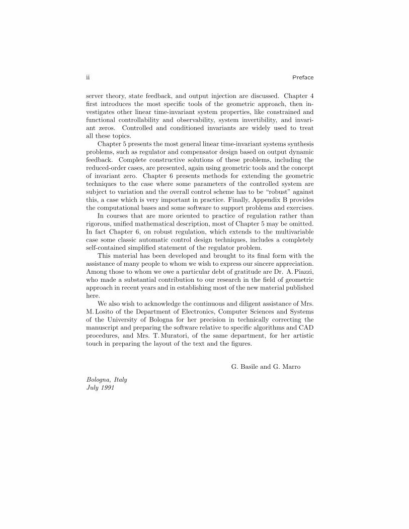
In order to reproduce and analyze the behavior of a system, it is necessaryto refer to a mathematical model which, generally with a certain approxima-tion, represents the links existing between the various measurable attributes orvariables of the system. The same system can be related to several mathemat-ical models, each of which may correspond to a different compromise betweenprecision and simplicity, and may also depend on the particular problem.
Since mathematical models are themselves systems, although abstract, it iscustomary to denote both the object of the study and its mathematical modelby the word “system.” The discipline called system theory pertains to thederivation of mathematical models for systems, their classification, investiga-tion of their properties, and their use for the solution of engineering problems.
A system can be represented as a block and its variables as connectionswith the environment or other systems, as shown by the simple diagram ofFig. 1.1.
As a rule, in order to represent a system with a mathematical model, itis first necessary to divide its variables into causes or inputs and effects oroutputs . Inputs correspond to independent and outputs to dependent variables.A system whose variables are so divided is called an oriented system and canbe represented as shown in Fig. 1.2, with the connections oriented by means ofarrows.
Σ
Figure 1.2. Schematic representation of an oriented system.
It is worth noting that the distinction between causes and effects appearsquite natural, so it is often tacitly assumed in studying physical systems;nevertheless in some cases it is anything but immediate. Consider, for instance,the simple electric circuit shown in Fig. 1.3(a), whose variables are v and i. Itcan be oriented as in Fig. 1.3(b), i.e., with v as input and i as output: this isthe most natural choice if the circuit is supplied by a voltage generator. Butthe same system may be supplied by a current generator, in which case i wouldbe the cause and v the effect and the corresponding oriented block diagram

1.2. Some Examples of Dynamic Systems 3
would be as shown in Fig. 1.3(c).
i
i
i v
v
v
R
L
Σ
Σ
(a)
(b)
(c)
Figure 1.3. An electric system with two possible orientations.
Systems can be divided into two main classes: memoryless or purely alge-braic systems, in which the values of the outputs at any instant of time dependonly on the values of the inputs at the same time, and systems with memory ordynamic systems , in which the values of the outputs depend also on the pasttime evolution of the inputs.
In dynamic systems the concept of state plays a fundamental role: inintuitive terms, the state of a system is the information that is necessary atevery instant of time, in order to be able to predict the effect of the past historyof the system on its future behavior. The state consists of a set of variables or, indistributed-parameter systems, of one or more functions of space coordinates,and is subject to variation in time depending on the time evolution of theinputs.
The terms “input,” “state,” and “output” of a system usually refer to all itsinput, state, and output variables as a whole, whereas the terms input function,output function, and motion refer to the time evolution of such variables. Inparticular, input and output functions are often called input and output signals ;the terms stimulus and response are also used.
A system that is not connected to the environment by any input is called afree or autonomous system; if, on the contrary, there exist any such inputs thatrepresent stimuli from the environment, they are called exogenous (variablesor signals) and it is said to be a forced system. In control problems, it is naturalto divide inputs into manipulable variables and nonmanipulable variables . Theformer are those whose values can be imposed at every instant of time in orderto achieve a given control goal. The latter are those that cannot be arbitrarilyvaried; if unpredictable, they are more precisely called disturbances .
1.2 Some Examples of Dynamic Systems
This section presents some examples of dynamic systems and their mathemat-ical models, with the aim of investigating their common features.

4 Chapter 1. Introduction to Systems
u
x
y
R1
R2
C
Figure 1.4. A simple electric circuit.
Example 1.2.1 (a simple electric circuit) Consider the electric circuit shownin Fig. 1.4. It is described by the equations, one differential and one algebraic,
x(t) = a x(t) + b u(t) (1.2.1)
y(t) = c x(t) + d u(t) (1.2.2)
where the functions on the right side are respectively called state velocityfunction and output function; u and y denote the input and output voltages,x the voltage across the capacitor, which can be assumed as the (only) statevariable, and x the time derivative dx/dt. Constants a, b, c, and d are relatedto the electric parameters shown in the figure by the following easy-to-deriverelations:
a := − 1
C(R1 +R2)b :=
1
C(R1 +R2)
c :=R1
R1 +R2d :=
R2
R1 +R2
(1.2.3)
The differential equation (1.2.1) is easily solvable. Let t0 and t1 (t1>t0) be twogiven instants of time, x0 the initial state, i.e., the state at t0 and u(·) a givenpiecewise continuous function of time whose domain is assumed to contain thetime interval [t0, t1]. The solution of equation (1.2.1) for t∈ [t0, t1] is expressedby
x(t) = x0 ea(t−t0) +
∫ t
t0
ea(t−τ) b u(τ) dτ (1.2.4)
as can be easily checked by direct substitution.1 Function (1.2.4) is called thestate transition function: it provides the state x(t) as a function of t, t0, x0,and u[t0, t]. By substituting (1.2.4) into (1.2.2) we obtain the so-called response
1 Recall the rule for the computation of the derivative of an integral depending on aparameter:
d
dt
∫ b(t)
a(t)f(x, t) dx = f
(b(t), t
)b− f
(a(t), t
)a+
∫ b(t)
a(t)f(x, t) dx
where
f(x, t) :=∂
∂tf(x, t)

1.2. Some Examples of Dynamic Systems 5
function
y(t) = c
(x0 e
a(t−t0) +
∫ t
t0
ea(t−τ) b u(τ) dτ
)+ d u(t) � (1.2.5)
ia
va
La Ra
ve
vc
ω, cm
cr
Figure 1.5. An electric motor.
Example 1.2.2 (an electromechanical system) Let us now consider theslightly more complicated electromechanical system shown in Fig. 1.5, i.e., anarmature-controlled d.c. electric motor. Its behavior is described by the follow-ing set of two differential equations, which express respectively the equilibriumof the voltages along the electric mesh and that of the torques acting on theshaft:
va(t) = Ra ia(t) + Lad iadt
(t) + vc(t) (1.2.6)
cm(t) = B ω(t) + Jdω
dt(t) + cr(t) (1.2.7)
In (1.2.6) va is the applied voltage, Ra and La the armature resistance andinductance, ia and vc the armature current and counter emf, while in (1.2.7) cmis the motor torque, B, J , and ω the viscous friction coefficient, the moment ofinertia, and the angular velocity of the shaft, and cr an externally applied loadtorque. If the excitation voltage ve is assumed to be constant, the followingtwo additional relations hold:
vc(t) = k1 ω(t) cm(t) = k2 ia(t) (1.2.8)
where k1 and k2 denote constant coefficients, which are numerically equal toeach other if the adopted units are coherent (volt and amp for voltages andcurrents, Nm and rad/sec for torques and angular velocities). Orient the systemassuming as input variables u1 := va, u2 := cr and as output variable y := θ, theangular position of the shaft, which is related to ω by the simple equation
dθ
dt(t) = ω(t) (1.2.9)

6 Chapter 1. Introduction to Systems
Then assume as state variables the armature current, the angular velocity, andthe angular position of the shaft, i.e., x1 := ia, x2 :=ω, x3 := θ. Equations (6–9)can be written in compact form (using matrices) as
x(t) = Ax(t) +B u(t) (1.2.10)
y(t) = C x(t) +Du(t) (1.2.11)
where2 x := (x1, x2, x3), u := (u1, u2) and
A :=
⎡⎣−Ra/La −k1/La 0
k2/J −B/J 00 1 0
⎤⎦ B :=
⎡⎣ 1/La 0
0 −1/J0 0
⎤⎦
C := [ 0 0 1 ] D := [ 0 0 ] �(1.2.12)
Note that the mathematical model of the electric motor has the samestructure as that of the simple electric circuit considered before, but with theconstants replaced by matrices. It is worth pointing out that such a structure iscommon to all lumped-parameter linear time-invariant dynamic systems, whichare the most important in connection with control problems, and will also bethe protagonists in this book. A further remark: the last term in equation(1.2.11) can be deleted, D being a null matrix. In fact, in this case the inputdoes not influence the output directly, but only through the state. Systemswith this property are very common and are called purely dynamic systems .
z1 qq1 z
u
Figure 1.6. A surge tank installation.
Example 1.2.3 (a hydraulic system) A standard installation for a hydroelec-tric plant can be represented as in Fig. 1.6: it consists of a reservoir, a conduitconnecting it to a surge tank, which in turn is connected to the turbines bymeans of a penstock. At the bottom of the surge tank there is a throttle, builtin order to damp the water level oscillations. Let z1 be the total elevation ofwater level in the reservoir, z that in the surge tank, F (z) the cross-sectionalarea of the surge tank, which is assumed to be variable, z2 the static head atthe end of the conduit, q the flow per second in the conduit, q1 that into the
2 Here and in the following the same symbol is used for a vector belonging to Rn and an× 1 matrix.

1.2. Some Examples of Dynamic Systems 7
surge tank, and u that in the penstock. Neglecting water inertia in the surgetank, it is possible to set up the equations
k2(z1(t)− z2(t)
)= k1 q(t) |q(t)| + q(t) (1.2.13)
z2(t)− z(t) = k3 q1(t) |q1(t)| (1.2.14)
z(t) = F (z) q1(t) (1.2.15)
q1(t) = q(t)− u(t) (1.2.16)
which can be referred to, respectively, as the conduit equation, the throttleequation, the surge tank equation, and the flow continuity equation; k1, k2, andk3 denote constants. By substituting for z2 and q1, the first-order differentialequations
q(t) = −k1 q(t) |q(t)| + k2
(z1(t)− z(t) −
k3(q(t)− u(t)
) ∣∣q(t)− u(t)∣∣) (1.2.17)
z(t) = F (z)(q(t)− u(t)
)(1.2.18)
are obtained. Let z2 be assumed as the output variable: this choice is consistentsince z2 is the variable most directly related to the power-delivering capabilityof the plant: it can be expressed by the further equation
z2(t) = z(t) + k3(q(t)− u(t)
) ∣∣q(t)− u(t)∣∣ (1.2.19)
If the water level elevation in the reservoir is assumed to be constant, theonly input is u, which is typically a manipulable variable. We choose as statevariables the flow per second in the conduit and the water level elevation inthe surge tank, i.e., x1 := q, x2 := z, and, as the only output variable the statichead at the penstock, i.e., y := z2. Equations (1.2.17–1.2.19) can be written inthe more compact form
x(t) = f(x(t), u(t)
)(1.2.20)
y(t) = g(x(t), u(t)
)(1.2.21)
where x := (x1, x2) and f , g are nonlinear continuous functions. �
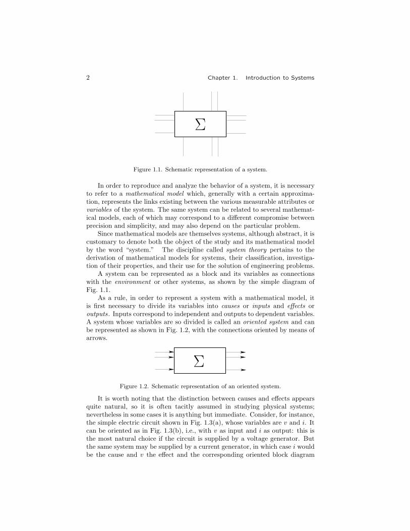
Example 1.2.4 (a distributed-parameter system) As an example of adistributed-parameter system, we consider the continuous furnace representedin Fig. 1.7(a): a strip of homogeneous material having constant cross-sectionalarea is transported with adjustable speed u through a furnace. Both the tem-perature distributions in the furnace and in the strip are assumed to be variablein the direction of movement z and uniform within sections orthogonal to thisdirection. Denote by f(z) the temperature along the furnace, which is assumedto be constant in time, and by x(t, z) that along the strip, which is a function of
8 Chapter 1. Introduction to Systems
u
z0 z1 zz z0 z1
f(z)
x(t, z)
(a) (b)
Figure 1.7. A continuous furnace and related temperature distributions.
both time and space. The system is described by the following one-dimensionalheat diffusion equation:
∂x(t, z)
∂t= k1
∂2x(t, z)
∂z2+ u(t)
∂x(t, z)
∂z+ k2
(x(t, z)− f(z)
)(1.2.22)
where k1 and k2 are constants related respectively to the internal and surfacethermal conductivity of the strip. We assume the speed u as the input variableand the temperature of the strip at the exit of the furnace as the output variable,i.e.,
y(t) = x(t, z1) (1.2.23)
The function x(t, ·) represents the state at time t; the partial differentialequation (1.2.23) can be solved if the initial state x(t0, ·) (initial condition),the strip temperature before heating x(·, z0) (boundary condition), usuallyconstant, and the input function u(·), are given. �
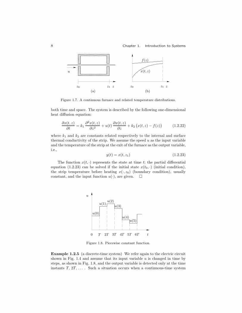
u
0 T 2T 3T 4T 5T 6T t
u(0)
u(1)u(2)
u(3)
u(4)u(5)
Figure 1.8. Piecewise constant function.
Example 1.2.5 (a discrete-time system) We refer again to the electric circuitshown in Fig. 1.4 and assume that its input variable u is changed in time bysteps, as shown in Fig. 1.8, and the output variable is detected only at the timeinstants T, 2T, . . . . Such a situation occurs when a continuous-time system

1.2. Some Examples of Dynamic Systems 9
is controlled by means of a digital processor, whose inputs and outputs aresampled data.
Denote by u(i ) the input value in the time interval [iT, (i + 1)T ) and byy(i ) the output value at the time iT ; the system is easily shown as beingdescribed by a difference equation and an algebraic equation, i.e.,
x(i+1) = ad x(i ) + bd u(i ) (1.2.24)
y(i ) = c x(i ) + d u(i ) (1.2.25)
where coefficients c and d are the same as in equation (1.2.2), whereas ad, bdare related to a, b and the sampling period T by
ad = eaT bd = b
∫ T
0
ea(T−τ) dτ =b
a
(eaT − 1
)(1.2.26)
Subscript d in the coefficients stands for “discrete.” In discrete-time systems,time is an integer variable instead of a real variable and time evolutions of thesystem variables are represented by sequences instead of continuous or piecewisecontinuous functions of time. Let j, i (i > j) be any two (integer) instants oftime, x0 the initial state, i.e., the state at time j, and u(·) the input sequencein any time interval containing [j, i].3 The state transition function is obtainedby means of a recursive application of (1.2.24) and is expressed by
x(i ) = adi−j x0 +
i−1∑k=1
adi−k−1 bd u(k) (1.2.27)
The response function is obtained by substituting (1.2.27) into (1.2.25) as
y(i ) = c
(ad
i−j x0 +i−1∑k=1
adi−k−1 bd u(k)
)+ d u(i ) � (1.2.28)
Example 1.2.6 (a finite-state system) The finite-state system is representedas a block in Fig. 1.9(a): the input variables u1, u2 are the positions of two pushbuttons and the output variable y is the lighting of a lamp. The value of eachvariable is represented by one of two symbols, for instance 1 or 0 accordingto whether the push buttons are pressed or released and whether the lampis lighted or not. The input data are assumed to be sampled, i.e., they areaccepted when a clock pulse is received by the system; also the possible outputvariable changes occur at clock pulses, so that their time evolution is inherentlydiscrete. The system behavior is described in words as follows: “lamp lights up
3 For the sake of precision, note that this time interval is necessary in connection withthe response function, but can be restricted to [j, i− 1] for the state transition function.
10 Chapter 1. Introduction to Systems
Σ
u1
u2
y
u1u2u1u2 f g
xx 0000 0101 1111 1010
00
0
00
00000 000
11 11 1
1
1
(a)
(b) (c)
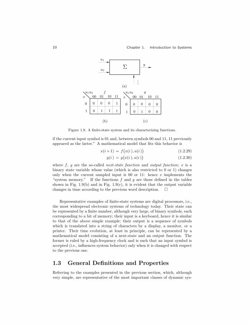
Figure 1.9. A finite-state system and its characterizing functions.
if the current input symbol is 01 and, between symbols 00 and 11, 11 previouslyappeared as the latter.” A mathematical model that fits this behavior is
x(i+1) = f(x(i ), u(i )
)(1.2.29)
y(i ) = g(x(i ), u(i )
)(1.2.30)
where f , g are the so-called next-state function and output function; x is abinary state variable whose value (which is also restricted to 0 or 1) changesonly when the current sampled input is 00 or 11: hence x implements the“system memory.” If the functions f and g are those defined in the tablesshown in Fig. 1.9(b) and in Fig. 1.9(c), it is evident that the output variablechanges in time according to the previous word description. �
Representative examples of finite-state systems are digital processors, i.e.,the most widespread electronic systems of technology today. Their state canbe represented by a finite number, although very large, of binary symbols, eachcorresponding to a bit of memory; their input is a keyboard, hence it is similarto that of the above simple example; their output is a sequence of symbolswhich is translated into a string of characters by a display, a monitor, or aprinter. Their time evolution, at least in principle, can be represented by amathematical model consisting of a next-state and an output function. Theformer is ruled by a high-frequency clock and is such that an input symbol isaccepted (i.e., influences system behavior) only when it is changed with respectto the previous one.
1.3 General Definitions and Properties
Referring to the examples presented in the previous section, which, althoughvery simple, are representative of the most important classes of dynamic sys-

1.3. General Definitions and Properties 11
tems, let us now state general definitions and properties in which the mostbasic connections between system theory and mathematics are shown.
First, consider the sets to which the variables and functions involved in thesystem mathematical model must belong. In general it is necessary to specify
1. a time set T2. an input set U3. an input function set Uf4. a state set X5. an output set Y
The values and functions belonging to the above sets are called admissi-ble. Only two possibilities will be considered for the time set: T =R (time ismeasured by a real number) and T =Z (time is measured by an integer num-ber). It is worth noting that the properties required for a set to be a time setfrom a strict mathematical viewpoint are fewer than the properties of eitherR or Z; for instance, multiplication does not need to be defined in a time set.Nevertheless, since the familiar R and Z fit our needs, it is convenient to adoptthem as the only possible time sets and avoid any subtle investigation in orderto find out what is strictly required for a set to be a time set. On the basis ofthis decision, the following definitions are given.
Definition 1.3.1 (continuous-time and discrete-time system) A system issaid to be continuous-time if T =R, discrete-time if T =Z.
Definition 1.3.2 (purely algebraic system) A memoryless or purely algebraicsystem is composed of sets T , U , Y, and an input-output function or input-output map:
y(t) = g(u(t), t
)(1.3.1)
Definition 1.3.3 (dynamic continuous-time system) A dynamic continuous-time system is composed of sets T (= R), U , Uf , X , Y of a state velocityfunction
x(t) = f(x(t), u(t), t
)(1.3.2)
having a unique solution for any admissible initial state and input function andof an output function or output map
y(t) = g(x(t), u(t), t
)(1.3.3)
Definition 1.3.4 (dynamic discrete-time system) A dynamic discrete-timesystem is composed of sets T (= Z), U , Uf , X , Y of a next-state function4
x(i+1) = f(x(i ), u(i ), i
)(1.3.4)
and of an output function or output map
y(i ) = g(x(i ), u(i ), i
)(1.3.5)
4 In the specific case of discrete-time systems, symbols i or k instead of t are used todenote time. However, in general definitions reported in this chapter, which refer both tothe continuous and the discrete-time case, the symbol t is used to denote a real as well as aninteger variable.
12 Chapter 1. Introduction to Systems
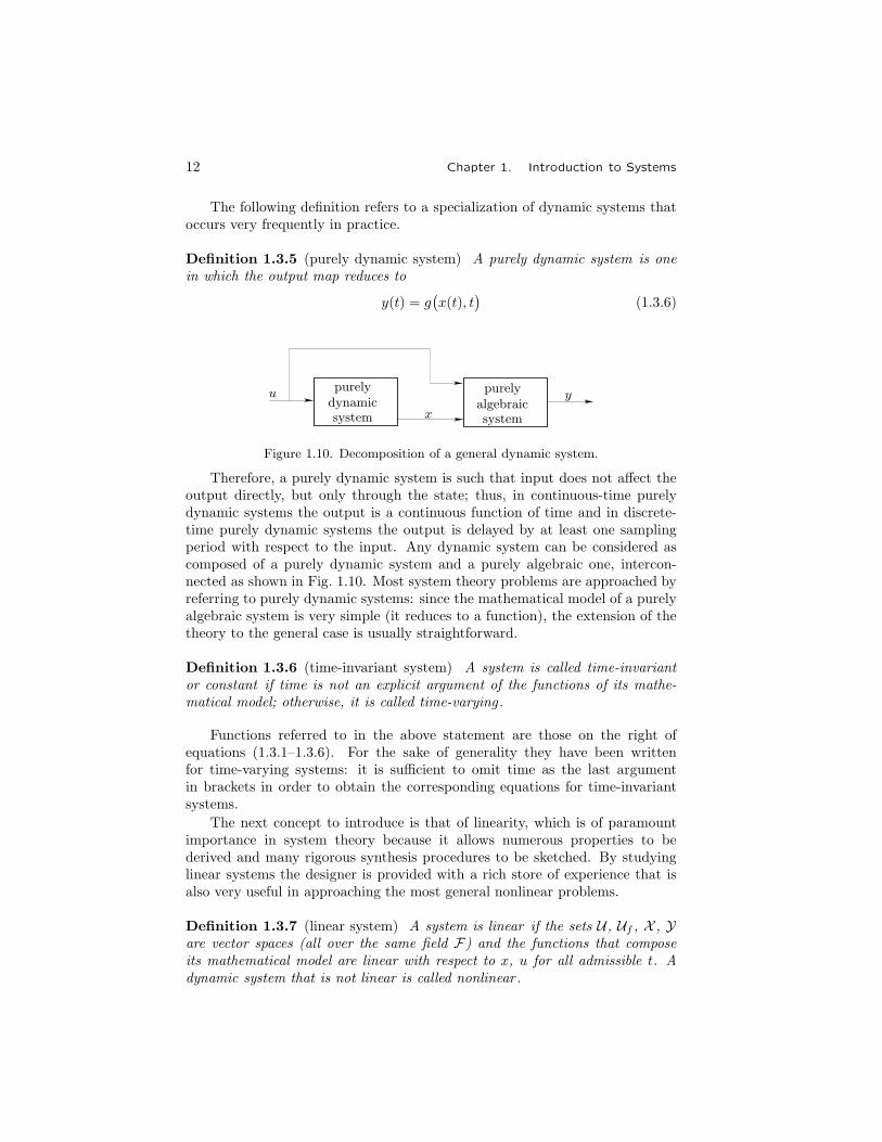
The following definition refers to a specialization of dynamic systems thatoccurs very frequently in practice.
Definition 1.3.5 (purely dynamic system) A purely dynamic system is onein which the output map reduces to
y(t) = g(x(t), t
)(1.3.6)
u
x
ypurelydynamicsystem
purelyalgebraicsystem
Figure 1.10. Decomposition of a general dynamic system.
Therefore, a purely dynamic system is such that input does not affect theoutput directly, but only through the state; thus, in continuous-time purelydynamic systems the output is a continuous function of time and in discrete-time purely dynamic systems the output is delayed by at least one samplingperiod with respect to the input. Any dynamic system can be considered ascomposed of a purely dynamic system and a purely algebraic one, intercon-nected as shown in Fig. 1.10. Most system theory problems are approached byreferring to purely dynamic systems: since the mathematical model of a purelyalgebraic system is very simple (it reduces to a function), the extension of thetheory to the general case is usually straightforward.
Definition 1.3.6 (time-invariant system) A system is called time-invariantor constant if time is not an explicit argument of the functions of its mathe-matical model; otherwise, it is called time-varying.
Functions referred to in the above statement are those on the right ofequations (1.3.1–1.3.6). For the sake of generality they have been writtenfor time-varying systems: it is sufficient to omit time as the last argumentin brackets in order to obtain the corresponding equations for time-invariantsystems.
The next concept to introduce is that of linearity, which is of paramountimportance in system theory because it allows numerous properties to bederived and many rigorous synthesis procedures to be sketched. By studyinglinear systems the designer is provided with a rich store of experience that isalso very useful in approaching the most general nonlinear problems.
Definition 1.3.7 (linear system) A system is linear if the sets U , Uf , X , Yare vector spaces (all over the same field F) and the functions that composeits mathematical model are linear with respect to x, u for all admissible t. Adynamic system that is not linear is called nonlinear.

1.3. General Definitions and Properties 13
As a consequence of the above definition, in the case of purely algebraiclinear systems instead of equation (1.3.1) we will consider the equation
y(t) = C(t)u(t) (1.3.7)
whereas in the case of continuous-time linear dynamic systems, instead ofequations (1.3.2, 1.3.3) we refer more specifically to the equations
x(t) = A(t)x(t) +B(t)u(t) (1.3.8)
y(t) = C(t)x(t) +D(t)u(t) (1.3.9)
In the above equations A(t), B(t), C(t), and D(t) denote matrices with el-ements depending on time which, in particular, are constant in the case oftime-invariant systems.
Similarly, for discrete-time linear dynamic systems instead of equations(1.3.4, 1.3.5) we refer to the equations
x(i+1) = Ad(i )x(i ) +Bd(i )u(i ) (1.3.10)
y(i ) = Cd(i )x(i ) +Dd(i )u(i ) (1.3.11)
where Ad(i ), Bd(i ), Cd(i ) and Dd(i ) are also matrices depending on discretetime that are constant in the case of time-invariant systems.
If, in particular, U :=Rp, X :=Rn, Y :=Rq, i.e., input, state, and output arerespectively represented by a p-tuple, an n-tuple, and a q-tuple of real numbers,A(t), B(t), C(t), D(t), and the corresponding symbols for the discrete-timecase can be considered to denote real matrices of proper dimensions, which arefunctions of time if the system is time-varying and constant if the system istime-invariant.
In light of the definitions just stated, let us again consider the six examplespresented in the previous section. The systems in Examples 1.2.1–1.2.4 arecontinuous-time, whereas those in Examples 1.2.5 and 1.2.6 are discrete-time.All of them are time-invariant, but may be time-varying if some of the pa-rameters that have been assumed to be constant are allowed to vary as givenfunctions of time: for instance, the elevation z1 of the water level in the reser-voir of the installation shown in Fig. 1.6 may be subject to daily oscillations(depending on possible oscillations of power request) or yearly oscillations ac-cording to water inlet dependence on seasons. As far as linearity is concerned,the systems considered in Examples 1.2.1, 1.2.2, and 1.2.5 are linear, whereasall the others are nonlinear.
The input sets are R, R2, R, R, R, B respectively, the state sets are R,R
3, R2, Rf , R, B, and the output sets are R, R, R, R, R, B. Rf denotes avector space of functions with values in R. Also the input function set Uf mustbe specified, particularly for continuous-time systems in order to guaranteethat the solutions of differential equation (1.3.2) have standard smoothnessand uniqueness properties. In general Uf is assumed to be the set of all thepiecewise continuous functions with values in U , but in some special cases, it
14 Chapter 1. Introduction to Systems
could be different: if, for instance, the input of a dynamic system is connectedto the output of a purely dynamic system, input functions of the former arerestricted to being continuous. In discrete-time systems in general Uf is asequence with values in U without any special restriction.
U
u2
u1
Figure 1.11. A possible input set contained in R2.
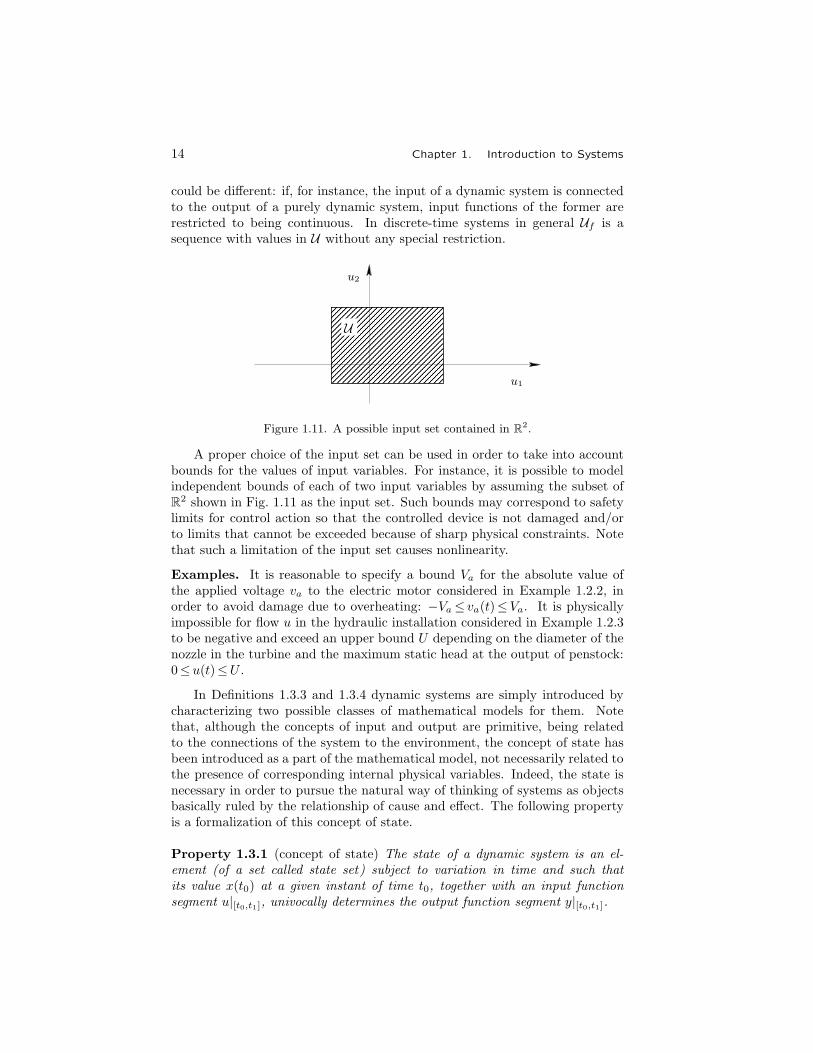
A proper choice of the input set can be used in order to take into accountbounds for the values of input variables. For instance, it is possible to modelindependent bounds of each of two input variables by assuming the subset ofR2 shown in Fig. 1.11 as the input set. Such bounds may correspond to safetylimits for control action so that the controlled device is not damaged and/orto limits that cannot be exceeded because of sharp physical constraints. Notethat such a limitation of the input set causes nonlinearity.
Examples. It is reasonable to specify a bound Va for the absolute value ofthe applied voltage va to the electric motor considered in Example 1.2.2, inorder to avoid damage due to overheating: −Va≤ va(t)≤Va. It is physicallyimpossible for flow u in the hydraulic installation considered in Example 1.2.3to be negative and exceed an upper bound U depending on the diameter of thenozzle in the turbine and the maximum static head at the output of penstock:0≤u(t)≤U .
In Definitions 1.3.3 and 1.3.4 dynamic systems are simply introduced bycharacterizing two possible classes of mathematical models for them. Notethat, although the concepts of input and output are primitive, being relatedto the connections of the system to the environment, the concept of state hasbeen introduced as a part of the mathematical model, not necessarily related tothe presence of corresponding internal physical variables. Indeed, the state isnecessary in order to pursue the natural way of thinking of systems as objectsbasically ruled by the relationship of cause and effect. The following propertyis a formalization of this concept of state.
Property 1.3.1 (concept of state) The state of a dynamic system is an el-ement (of a set called state set) subject to variation in time and such thatits value x(t0) at a given instant of time t0, together with an input functionsegment u|[t0,t1], univocally determines the output function segment y|[t0,t1].
1.3. General Definitions and Properties 15
Property 1.3.1 implies the property of causality: all dynamic systems whichare considered in this book are causal or nonanticipative, i.e., their output atany instant of time t does not depend on the values of input at instants of timegreater than t.
The nature of the state variables deeply characterizes dynamic systems, sothat it can be assumed as a classification for them, according to the followingdefinition.
Definition 1.3.8 (finite-state or finite-dimensional system) A dynamic sys-tem is called finite-state, finite-dimensional , infinite-dimensional if its stateset is respectively a finite set, a finite-dimensional vector space, or an infinite-dimensional vector space.
A more compact mathematical description of dynamic system behavior isobtained as follows: equation (1.3.2) – by assumption – and equation (1.3.4)– by inherent property – have a unique solution that can be expressed as afunction of the initial instant of time t0, the initial state x0 := x(t0), and theinput function u(·), that is:
x(t) = ϕ(t, t0, x0, u(·)
)(1.3.12)
Function ϕ is called the state transition function. Being the solution of adifferential or a difference equation, it has some special features, such as:
1. time orientation: it is defined for t≥ t0, but not necessarily for t< t0;
2. causality: its dependence on the input function is restricted to the timeinterval [t0, t]:
ϕ(t, t0, x0, u1(·)
)= ϕ
(t, t0, x0, u2(·)
)if u1|[t0,t] =u2|[t0,t]
3. consistency:x = ϕ
(t, t, x, u(·)
)4. composition: consecutive state transitions are congruent. i.e.,
ϕ(t, t0, x0, u(·)
)= ϕ
(t, t1, x1, u(·)
)provided that
x1 := ϕ(t1, t0, x0, u(·)
), t0 ≤ t1 ≤ t
The pair (t, x(t))∈ T ×X is called an event : when the initial event(t0, x(t0)) and the input function u(·) are known, the state transition func-tion provides a set of events, namely a function x(·) : T →X , which is calledmotion. To be precise, the motion in the time interval [t0, t1] is the set{
(t, x(t)) : x(t)=ϕ(t, t0, x(t0), u(·)
), t∈ [t0, t1]
}(1.3.13)
The image of motion in the state set, i.e., the set{x(t) : x(t)=ϕ
(t, t0, x(t0), u(·)
), t∈ [t0, t1]
}(1.3.14)

16 Chapter 1. Introduction to Systems
x
x(0)
0
0
t1
t1
t2
t2
t
t
u
(a)
(b)
Figure 1.12. A possible motion and the corresponding input function.
of all the state values in the time interval [t0, t1] is called the trajectory (of thestate in [t0, t1]).
When the state set X coincides with a finite-dimensional vector spaceR
n, the motion can be represented as a line in the event space T ×X andthe trajectory as a line in the state space X , graduated versus time. Therepresentation in the event space of a motion of the electric circuit described inExample 1.2.1 and the corresponding input function are shown in Fig. 1.12,while the representation in the state space of a possible trajectory of theelectromechanical system described in Example 1.2.2 and the correspondinginput function are shown in Fig. 1.13. For any given initial state differentinput functions cause different trajectories, all initiating at the same point ofthe state space; selecting input at a particular instant of time (for instance,t3) allows different orientations in space of the tangent to the trajectory at t3,namely of the state velocity (x1, x2, x3).
The analysis of dynamic system behavior mainly consists of studying tra-jectories and the possibility of influencing them through the input. Then thegeometric representation of trajectories is an interesting visualization of thestate transition function features and limits. In particular, it clarifies statetrajectory dependence on input.
Substituting (1.3.12) into (1.3.3) or (1.3.5) yields
y(t) = γ(t, t0, x0, u|[t0,t]
)t ≥ t0 (1.3.15)
Function γ is called the response function and provides the system output

1.3. General Definitions and Properties 17
x3
t
t
t1
t1
x(0)
0
0
t2
t2
t3
t3
x1
x2
u
(a)
(b)
Figure 1.13. A possible trajectory and the corresponding input function.
at generic time t as a function of the initial instant of time, the initial state,and a proper input function segment. Therefore equation (1.3.15) representsthe relationship of cause and effect which characterizes the time behavior of adynamic system and can be considered as an extension of the cause and effectrelationship expressed by (1.3.1) for memoryless systems. Equation (1.3.15)expresses a line in the output space, which is called output trajectory.
A very basic concept in system theory is that of the minimality of an input-state-output mathematical representation.
Definition 1.3.9 (indistinguishable states) Consider a dynamic system. Twostates x1, x2 ∈X are called indistinguishable in [t0, t1] if
γ(t, t0, x1, u(·)
)= γ
(t, t0, x2, u(·)
)∀ t ∈ [t0, t1] , ∀ u(·) ∈ Uf (1.3.16)
Definition 1.3.10 (equivalent states) Consider a dynamic system. Twostates x1, x2 ∈X that are indistinguishable in [t0, t1] ∀ t0, t1 ∈T , t1>t0 arecalled equivalent.
Definition 1.3.11 (minimal system) A dynamic system that has no equiva-lent states is said to be in minimal form or, simply, minimal.
Any nonminimal dynamic system can be made minimal by defining a newstate set in which every new state corresponds to a class of equivalent old states,and by redefining the system functions accordingly.

18 Chapter 1. Introduction to Systems
Definition 1.3.12 (equivalent systems) Two dynamic systems Σ1, Σ2
are said to be equivalent if they are compatible (i.e., if T1 = T2, U1 =U2,Uf1 =Uf2 =Uf , Y1 =Y2) and to any state x1 ∈X1 of Σ1 it is possible to asso-ciate a state x2 ∈X2 of Σ2, and vice versa, such that 5
γ1(t, t0, x1, u(·)
)= γ2
(t, t0, x2, u(·)
)∀ t0 , ∀ t≥ t0 , ∀u(·)∈Uf (1.3.17)
In some control problems it is necessary to stop the time evolution of thestate of a dynamic system at a particular value. This is possible only if such avalue corresponds to an equilibrium state according to the following definition.
Definition 1.3.13 (temporary equilibrium state) In a dynamic system anystate x∈X is a temporary equilibrium state in [t0, t1] if there exists an admis-sible input function u(·)∈Uf such that
x = ϕ(t, t0, x, u(·)
)∀ t ∈ [t0, t1] (1.3.18)
The state x is called simply an equilibrium state if it is a temporary equilibriumstate in [t0, t1] for all the pairs t0, t1 ∈T , t1>t0.
Note that, owing to the property of time-shifting of causes and effects, intime-invariant systems all temporary equilibrium states in any finite time in-terval are simply equilibrium states. Referring to the geometric representationof the state evolution as a state space trajectory, equilibrium states are oftenalso called equilibrium points .
When the corresponding dynamic system is either time-invariant or linear,functions ϕ and γ have special properties, which will now be investigated.
Property 1.3.2 (time-shifting of causes and effects) Let us consider a time-invariant system and for any τ ∈T and all the input functions u(·)∈Uf definethe shifted input function as
uΔ(t+ τ) := u(t) ∀ t ∈ T (1.3.19)
assume that uΔ(·) ∈ Uf for all u(·) ∈ Uf , i.e., that the input function set isclosed with respect to the shift operation. The state transition function and theresponse function satisfy the following relationships:
x(t) = ϕ(t, t0, x0, u(·)
)⇔ x(t) = ϕ
(t+ τ, t0 + τ, x0, uΔ(·)
)(1.3.20)
y(t) = γ(t, t0, x0, u(·)
)⇔ y(t) = γ
(t+ τ, t0 + τ, x0, uΔ(·)
)(1.3.21)
Proof. We refer to system equations (1.3.2, 1.3.3) or (1.3.4, 1.3.5) and assumethat the system is time-invariant, so that functions on the right are independentof time. The property is a consequence of the fact that shifting any function oftime implies also shifting its derivative (in the case of continuous-time systems)or all future values (in the case of discrete-time systems), so that equations arestill satisfied if all the involved functions are shifted. �
5 If Σ1 e Σ2 are both in minimal form, this correspondence between initial states is clearlyone-to-one.
1.3. General Definitions and Properties 19
Assuming in equations (1.3.20) and (1.3.21) τ := − t0, we obtain
x(t) = ϕ(t, t0, x0, u(·)
)⇔ x(t) = ϕ
(t− t0, 0, x0, uΔ(·)
)y(t) = γ
(t, t0, x0, u(·)
)⇔ y(t) = γ
(t− t0, 0, x0, uΔ(·)
)from which it can be inferred that
1. when the system referred to is time-invariant, the initial instant of timecan be assumed to be zero without any loss of generality;
2. the state transition and response functions of time-invariant systems areactually dependent on the difference t− t0 instead of t and t0 separately.
Property 1.3.3 (linearity of state transition and response functions) Let usconsider a linear dynamic system and denote by α, β any two elements ofthe corresponding field F , by x01, x02 any two admissible initial states and byu1(·), u2(·) any two admissible input function segments. The state transitionand response functions satisfy the following relationships:
ϕ(t, t0, α x01 + β x02, α u1(·)+ β u2(·)
)=
αϕ(t, t0, x01, u1(·)
)+ β ϕ
(t, t0, x02, u2(·)
)(1.3.22)
γ(t, t0, α x01 +β x02, α u1(·)+ β u2(·)
)=
αγ(t, t0, x01, u1(·)
)+ β ϕ
(t, t0, x02, u2(·)
)(1.3.23)
which express the linearity of ϕ and γ with respect to the initial state and inputfunction.
Proof. We refer to equation (1.3.8) or (1.3.10) and consider its solutionscorresponding to the different pairs of initial state and input function segmentsx01, u1(·) and x2, u2(·), which can be expressed as
x1(t) = ϕ(t, t0, x01, u1(·)
)x2(t) = ϕ
(t, t0, x02, u2(·)
)By substituting on the right of (1.3.8) or (1.3.10) αx1(t)+ β x2(t),αu1(t)+ β u2(t) in place of x(t), u(t) and using linearity, we obtain on the leftthe quantity α x1(t)+ β x2(t) in the case of (1.3.8), or αx1(t+1) + β x2(t+1)in the case of (1.3.10). Therefore, αx1(t)+ β x2(t) is a solution of the differ-ential equation (1.3.8) or difference equation (1.3.10); hence (1.3.22) holds. Asa consequence, (1.3.23) also holds, provided that γ is the composite functionof two linear functions. �
In the particular case α= β=1, equations (1.3.22, 1.3.23) correspond to theso-called property of superposition of the effects .

20 Chapter 1. Introduction to Systems
Property 1.3.4 (decomposability of state transition and response functions)In linear systems the state transition (response) function corresponding to theinitial state x0 and the input function u(·) can be expressed as the sum of thezero-input state transition (response) function corresponding to the initial statex0 and the zero-state state transition (response) function corresponding to theinput function u(·).Proof. Given any admissible initial state x0 and any admissible input functionu|[t0,t], assume in equations (1.3.22, 1.3.23), α := 1, β := 1, x01 :=x0, x02 := 0,u1(·) := 0, u2(·) := u(·); it follows that
ϕ(t, t0, x0, u(·)
)= ϕ(t, t0, x0, 0) + ϕ
(t, t0, 0, u(·)
)(1.3.24)
γ(t, t0, x0, u(·)
)= γ(t, t0, x0, 0) + γ
(t, t0, 0, u(·)
)� (1.3.25)
The former term of the above decomposition is usually referred to as the freemotion (free response), the latter as the forced motion (forced response). Thefollowing properties are immediate consequences of the response decompositionproperty.
Property 1.3.5 Two states of a linear system are indistinguishable in [t0, t1]if and only if they generate the same free response in [t0, t1].
Property 1.3.6 A linear system is in minimal form if and only if for anyinitial instant of time t0 no different states generate the same free response.
1.4 Controlling and Observing the State
The term controllability denotes the possibility of influencing the motion x(·)or the response y(·) of a dynamical system Σ by means of the input function(or control function) u(·)∈Uf .
In particular, one may be required to steer a system from a state x0 to x1or from an event (t0, x0) to (t1, x1): if this is possible, the system is said to becontrollable from x0 to x1 or from (t0, x0) to (t1, x1). Equivalent statementsare: “the state x0 (or the event (t0, x0)) is controllable to x1 (or to (t1, x1))”and “the state x1 (or the event (t1, x1)) is reachable from x0 (or from (t0, x0)).”
Example. Suppose the electric motor in Fig. 1.5 is in a given state x0 att=0: a typical controllability problem is to reach the zero state (i.e., to nullthe armature current, the angular velocity, and the angular position) at a timeinstant t1, (which may be specified in advance or not), by an appropriate choiceof the input function segment u|[0,t1]; if this problem has a solution, state x0 issaid to be controllable to the zero state (in the time interval [t0, t1]).
Controllability analysis is strictly connected to the definition of particularsubsets of the state space X , that is:
1. the reachable set at the final time t= t1 from the event (t0, x0)
R+(t0, t1, x0) :={x1 : x1 = ϕ
(t1, t0, x0, u(·)
), u(·)∈Uf
}(1.4.1)
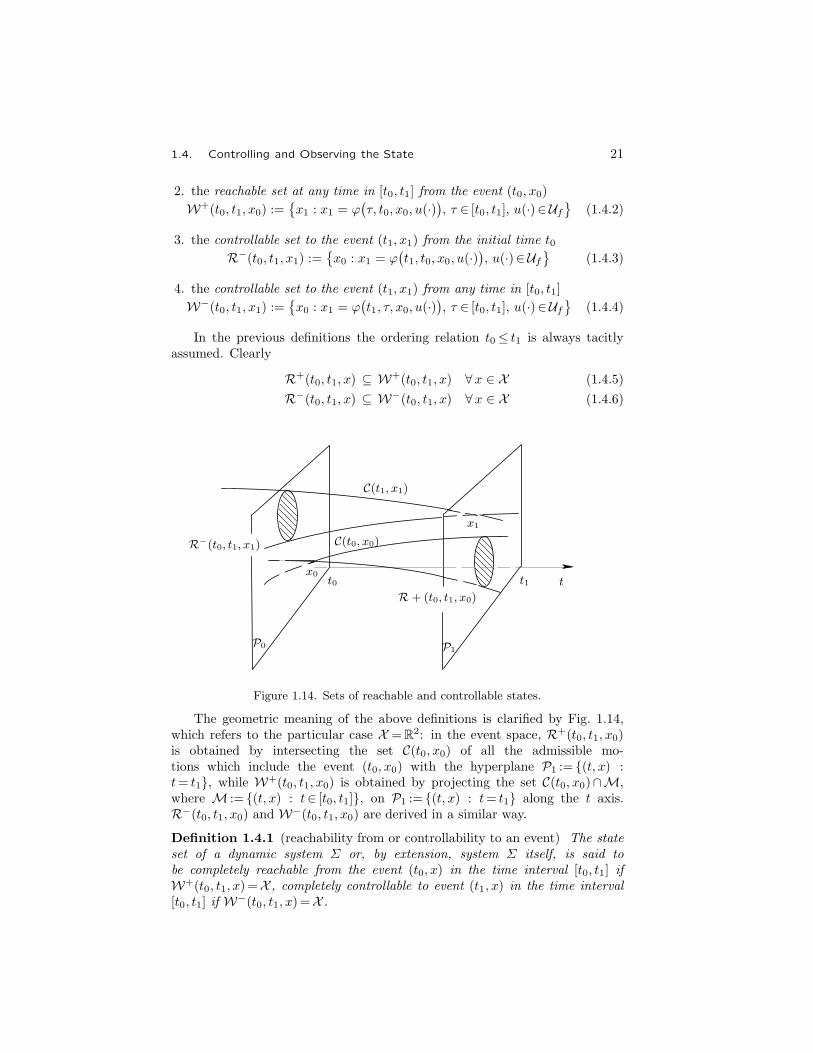
1.4. Controlling and Observing the State 21
2. the reachable set at any time in [t0, t1] from the event (t0, x0)
W+(t0, t1, x0) :={x1 : x1 = ϕ
(τ, t0, x0, u(·)
), τ ∈ [t0, t1], u(·)∈Uf
}(1.4.2)
3. the controllable set to the event (t1, x1) from the initial time t0R−(t0, t1, x1) :=
{x0 : x1 = ϕ
(t1, t0, x0, u(·)
), u(·)∈Uf
}(1.4.3)
4. the controllable set to the event (t1, x1) from any time in [t0, t1]
W−(t0, t1, x1) :={x0 : x1 = ϕ
(t1, τ, x0, u(·)
), τ ∈ [t0, t1], u(·)∈Uf
}(1.4.4)
In the previous definitions the ordering relation t0≤ t1 is always tacitlyassumed. Clearly
R+(t0, t1, x) ⊆ W+(t0, t1, x) ∀x ∈ X (1.4.5)
R−(t0, t1, x) ⊆ W−(t0, t1, x) ∀x ∈ X (1.4.6)
R−(t0, t1, x1)
C(t1, x1)
C(t0, x0)
x1
x0t0
R+ (t0, t1, x0)
P0 P1
t1 t
Figure 1.14. Sets of reachable and controllable states.
The geometric meaning of the above definitions is clarified by Fig. 1.14,which refers to the particular case X =R
2: in the event space, R+(t0, t1, x0)is obtained by intersecting the set C(t0, x0) of all the admissible mo-tions which include the event (t0, x0) with the hyperplane P1 := {(t, x) :t= t1}, while W+(t0, t1, x0) is obtained by projecting the set C(t0, x0)∩M,where M := {(t, x) : t∈ [t0, t1]}, on P1 := {(t, x) : t= t1} along the t axis.R−(t0, t1, x0) and W−(t0, t1, x0) are derived in a similar way.
Definition 1.4.1 (reachability from or controllability to an event) The stateset of a dynamic system Σ or, by extension, system Σ itself, is said tobe completely reachable from the event (t0, x) in the time interval [t0, t1] ifW+(t0, t1, x)=X , completely controllable to event (t1, x) in the time interval[t0, t1] if W−(t0, t1, x)=X .

22 Chapter 1. Introduction to Systems
In time-invariant systems, R+(t0, t1, x), W+(t0, t1, x), R−(t0, t1, x),W−(t0, t1, x) do not depend on t0, t1 in a general way, but only on the dif-ference t1− t0, so that the assumption t0 =0 can be introduced without anyloss of generality and notation is simplified as:
1. R+t1(x): the reachable set at t= t1 from the event (0, x);
2. W+t1(x): the reachable set at any time in [0, t1] from the event (0, x);
3. R−t1(x): the controllable set to x at t= t1 from the initial time 0;
4. W−t1 (x): the controllable set to x at any time in [0, t1] from initial time 0.
Given any two instants of time t1, t2 satisfying t1≤ t2, the following hold:
W+t1(x) ⊆ W
+t2(x) ∀x ∈ X (1.4.7)
W−t1 (x) ⊆ W−t2 (x) ∀x ∈ X (1.4.8)
Notations W+(x), W−(x) refer to the limits
W+(x) := limt→∞
W+t (x) W−(x) := lim
t→∞W−t (x)
i.e., denote the reachable set from x and the controllable set to x in an arbitrarilylarge interval of time.
Definition 1.4.2 (completely controllable system) A time-invariant systemis said to be completely controllable or connected if it is possible to reach anystate from any other state (so that W+(x)=W−(x)=X for all x∈X ).
Consider now the state observation. The term observability denotes gener-ically the possibility of deriving the initial state x(t0) or the final state x(t1)of a dynamic system Σ when the time evolutions of input and output in thetime interval [t0, t1] are known. Final state observability is denoted also withthe term reconstructability. The state observation and reconstruction problemsmay not always admit a solution: this happens, in particular, for observationwhen the initial state belongs to a class whose elements are indistinguishablein [t0, t1].
Like controllability, observability is also analyzed by considering propersubsets of the state set X , which characterize dynamic systems regarding thepossibility of deriving state from input and output evolutions, i.e.:
1. the set of all the initial states consistent with the functions u(·), y(·) in thetime interval [t0, t1]
Q−(t0, t1, u(·), y(·)
):=
{x0 : y(τ) = γ
(τ, t0, x0, u(·)
), τ ∈ [t0, t1]
}(1.4.9)
2. the set of all the final states consistent with the functions u(·), y(·) in thetime interval [t0, t1]
Q+(t0, t1, u(·), y(·)
):={
x1 : x1 = ϕ(t1, t0, x0, u(·)
), x0 ∈Q−
(t0, t1, u(·), y(·)
)}(1.4.10)

1.4. Controlling and Observing the State 23
It is clear that in relations (1.4.9) and (1.4.10) y(·) is not arbitrary, butconstrained to belong to the set of all the output functions admissible withrespect to the initial state and the input function. This set is defined by
Yf(t0, u(·)
):=
{y(·) : y(t) = γ
(t, t0, x0, u(·)
), t≥ t0 , x0 ∈X
}(1.4.11)
Definition 1.4.3 (diagnosis or homing of a system) The state set of a dy-namic system Σ or, by extension, system Σ itself, is said to be observable in[t0, t1] by a suitable experiment (called diagnosis) if there exists at least oneinput function u(·)∈Uf such that the set (1.4.9) reduces to a single elementfor all y(·)∈Yf (t0, u(·)); it is said to be reconstructable in [t0, t1] by a suitableexperiment (called homing) if there exists at least one input function u(·)∈Ufsuch that the set (1.4.10) reduces to a single element for all y(·)∈Yf (t0, u(·)).
A dynamic system without any indistinguishable states in [t0, t1] is notnecessarily observable in [t0, t1] by a diagnosis experiment since different inputfunctions may be required to distinguish different pairs of initial states. This istypical in finite-state systems and quite common in general nonlinear systems.
Definition 1.4.4 (completely observable or reconstructable system) Thestate set of a dynamic system Σ or, by extension, system Σ itself, is said to becompletely observable in [t0, t1] if for all input functions u(·)∈Uf and for alloutput functions y(·)∈Yf (t0, u(·)) the set (1.4.9) reduces to a single element;it is said to be completely reconstructable in [t0, t1] if for all input functionsu(·)∈Uf and for all output functions y(·)∈Yf (t0, u(·)) the set (1.4.10) reducesto a single element.
Since the final state is a function of the initial state and input, clearly everysystem that is observable by a suitable experiment is also reconstructable bythe same experiment and every completely observable system is also completelyreconstructable.
In time-invariant systems Q−(t0, t1, u(·), y(·)) and Q+(t0, t1, u(·), y(·)) donot depend on t0 and t1 in a general way, but only on the difference t1− t0,so that, as in the case of controllability, the assumption t0 =0 can be intro-duced without any loss of generality. In this case the simplified notationsQ−t1(u(·), y(·)), Q
+t1(u(·), y(·)) will be used.
The above sets are often considered in solving problems related to systemcontrol and observation. The most significant of these problems are:
1. Control between two given states: given two states x0 and x1 andtwo instants of time t0 and t1, determine an input function u(·) such thatx1 =ϕ(t1, t0, x0, u(·)).2. Control to a given output : given an initial state x0, an output valuey1 and two instants of time t0, t1, t1>t0, determine an input u(·) such thaty1 = γ(t1, t0, x0, u(·)).3. Control for a given output function: given an initial state x0, an admissible
output function y(·) and two instants of time t0, t1, t1>t0, determine an inputu(·) such that y(t)= γ(t, t0, x0, u(·)) for all t∈ [t0, t1].

24 Chapter 1. Introduction to Systems
4. State observation: given corresponding input and output functionsu(·), y(·) and two instants of time t0, t1, t1>t0, determine an initial statex0 (or the whole set of initial states) consistent with them, i.e., such thaty(t)= γ(t, t0, x0, u(·)) for all t∈ [t0, t1].5. State reconstruction: given corresponding input and output functions u(·),y(·) and two instants of time t0, t1, t1>t0, determine a final state x1 (or thewhole set of final states) consistent with them, i.e., corresponding to an initialstate x0 such that x1 =ϕ(t1, t0, x0, u(·)), y(t)= γ(t, t0, x0, u(·)) for all t∈ [t0, t1].6. Diagnosis : like 4, except that the solution also includes the choice of a
suitable input function.
7. Homing: like 5, except that the solution also includes the choice of asuitable input function.
Moreover, problems often arise where observation and control are simulta-neously required. For instance, problems 1 and 2 would be of this type if initialstate x0 was not given.
1.5 Interconnecting Systems
Decomposing complex systems into simpler interconnected subsystems makestheir analysis easier. It is useful because many properties of the overall systemare often determined by analyzing corresponding properties of subsystems.Furthermore, it is convenient to keep different types of devices distinct, forinstance those whose behavior can be influenced by a suitable design (likecontrollers and, more generally, signal processors), and those that, on thecontrary, cannot be affected in any way.
1.5.1 Graphic Representations of Interconnected Sys-tems
Complex systems consisting of numerous interconnected parts are generallyrepresented in drawings by means of block diagrams and signal-flow graphs .They will be adopted here too, so, although they are very well known, it seemsconvenient to briefly recall their distinguishing features and interpretative con-ventions.
Block diagrams. Block diagrams are a convenient representation forsystems that consist of numerous interconnected parts. In this book they willbe used in a rather informal way: they will be referred without any graphicdifference to the single-variable as well as to the multivariable case, and themathematical model of the subsystem represented with a single block will bereported inside the block not in a unified way, but in the form that is mostconsistent with the text.
The main linkage elements between blocks are the branching point , repre-sented in Fig. 1.15(a) and the summing junction, represented in Fig. 1.16(b).

1.5. Interconnecting Systems 25
Figure 1.15. Branching point and summing junction.
Figure 1.16. Some types of blocks.
They are described respectively by the simple relations
y(t) = x(t)
z(t) = x(t)
andz(t) = x(t) + y(t)
Some types of blocks are shown in Fig. 1.16(a–e): block (a) representsthe linear purely algebraic constant input-output relation y=K u, where Kis a real constant or a real matrix; (b) and (c) represent nonlinear purelyalgebraic constant input-output relations, specifically a saturation or a blockof saturations and an ideal relay or block of ideal relays (or signum functions): ifreferred to multivariable cases, they are understood to have the same number ofoutputs as inputs; (d) represents a dynamic link specified by means of a transferfunction in the single-variable case or a transfer matrix in the multivariablecase; (e) a dynamic link specified by an ISO description: note, in this case,the possible presence of a further input denoting the initial state. In someblock diagrams, as for instance those shown in Fig. 1.10 and 1.25 to 1.27, nomathematical model is specified inside the blocks, but simply a description in

26 Chapter 1. Introduction to Systems
words of the corresponding subsystem. When, on the other hand, a precisemathematical description is given for each block of a diagram, the completediagram is equivalent to a set of equations for the overall system, in whichinterconnection equations are those of branching points and summing junctions.
Signal-flow graphs. Signal-flow graphs are preferred to block diagramsto represent complex structures consisting of several elementary (single-inputsingle-output) parts, each described by a transfer constant or a transfer func-tion. Their use is restricted to show the internal structure of some linearsystems which, although possibly of the multivariable type, can be representedas a connection of single-variable elements. The major advantage of signal-flowgraphs over block diagrams is that the transfer constant or the transfer func-tion relating any input to any output can be derived directly from a simpleanalysis of the topological structure of the graph.
A signal-flow graph is composed of branches and nodes . Every branchjoins two nodes in a given direction denoted by an arrow, i.e., is oriented andcharacterized by a coefficient or transfer function, called transmittance or gain.Every node represents a signal , which by convention is expressed by a linearcombination of the signals from whose nodes there exist branches directed toit, with the transmittances of these branches as coefficients. A node that hasno entering branches is called an independent or input node, while the othernodes are called dependent nodes : clearly, every dependent node represents alinear equation, so that the graph is equivalent to as many linear equations inas many unknowns as there are dependent nodes.
Figure 1.17. A signal-flow graph.
As an example, consider the simple signal-flow graph represented inFig. 1.17: transmittances are denoted by a, b, c, d, e, f, g, h and can be realconstants or transfer functions. The graph corresponds to the set of linearequations
x1 = a x0 + hx4 (1.5.1)
x2 = b x1 + g x2 + f x4 (1.5.2)
x3 = e x1 + c x2 (1.5.3)

1.5. Interconnecting Systems 27
x4 = d x3 (1.5.4)
in the unknowns x1, x2, x3, x4.Choose x4 as the output signal: we can derive a gain that relates x4 to
x0 by solving equations (1.5.1–1.5.4). Otherwise, we can take advantage ofthe relative sparseness of the signal-flow graph (in the sense that nodes arenot connected by branches in all possible ways) to use a topological analysismethod which in most practical cases turns out to be very convenient.
For this, some further definitions are needed. A path joining two givennodes is a sequence of adjacent branches that originates in the first node andterminates in the second passing through any node only once. The transmit-tance of a path P is the product of the transmittances of all the branches in thepath. A loop is a closed path. The transmittance of a loop L is the product ofthe transmittances of all the branches in the loop. A loop consisting of a singlebranch and a single node, as for instance loop g in Fig. 1.17, is called a self-loop.Two paths or two loops, or a path and a loop are said to be nontouching ifthey do not have any common node.
The Mason formula allows determination of the gain relating any depen-dent node to any source node of a signal-flow graph as a function of the trans-mittances of all the paths joining the considered nodes and all loops in thegraph. In order to express the formula, a little topological analysis is needed:denote by Pi, i∈P , where Jp is a set of indexes, the transmittances of allthe different paths joining the considered nodes; by Lj, j ∈J1, those of all thedifferent loops in the graph; by J2 the set of the pairs of indices correspond-ing to nontouching loops; by J3 that of the triples of indices corresponding tonontouching loops by three, and so on; furthermore, let J1,i be the set of theindices of all the loops not touching path Pi; J2,i that of the indices of all thepairs of nontouching loops not touching path Pi, and so on. When a set ofindexes is empty, so are all subsequent ones.
The Mason formula for the transmittance coefficient relating the considerednodes is
T =1
Δ
∑i∈Jp
PiΔi (1.5.5)
where
Δ := 1−∑i∈J1
Li +∑
(i,j)∈J2
Li Lj −∑
(i,j,k)∈J3
Li Lj Lk + . . . (1.5.6)
Δi := 1−∑
i∈J1,i
Li +∑
(i,j)∈J2,i
Li Lj −∑
(i,j,k)∈J3,i
Li Lj Lk + . . . (1.5.7)
Δ is called the determinant of the graph, whereas Δi denotes the determi-nant of the partial graph obtained by deleting the path Pi, i.e., by deleting allnodes belonging to Pi and all pertinent branches.
Going back to the example of Fig. 1.17, in order to derive the gain T relatingx4 to x0, first identify all paths and loops and determine their transmittances:
P1 = abcd , P2 = aed , P3 = abf

28 Chapter 1. Introduction to Systems
L1 = edh , L2 = bcdh , L3 = bfh , L4 = g
then consider the corresponding nonempty index sets:
Jp = {1, 2, 3} , J1 = {1, 2, 3, 4} , J2 = {(1, 4)} , J12 = {4}
The Mason formula immediately yields
T =abcd+ aed (1−g) + abf
1− edh− bcdh− bfh− g + edhg
1.5.2 Cascade, Parallel, and Feedback Interconnections
It is useful to define three basic interconnections of systems, which are oftenreferred to when considering decomposition problems.
Figure 1.18. Cascaded systems.
1. Cascade. Two dynamic systems Σ1 and Σ2 are said to be connectedin cascade (or, briefly, cascaded) if, at any instant of time, the input of Σ2
is a function of the output of Σ1, as shown in Fig. 1.18. For the cascadeconnection to be possible, condition T1 =T2 is necessary. The input set of theoverall system is U =U1, whereas the output set is Y =Y2 and the state set isX =X1×X2.
Figure 1.19. Parallel systems.
2. Parallel . Two dynamic systems Σ1 and Σ2 are said to be connected inparallel if, at any instant of time, their inputs are functions of a single variableu∈U , which is the input of the overall system, while the output y∈Y of theoverall systems is, at any instant of time, a function of both outputs y1 and

1.5. Interconnecting Systems 29
Figure 1.20. Feedback-connected systems.
y2. Condition T1 =T2 is also required in this case; the state set of the overallsystem is X =X1×X2. The parallel connection is shown in Fig. 1.19.
3. Feedback . Two dynamic systems Σ1 and Σ2 are said to be connected inmutual feedback if, at any instant of time, their inputs u1 and u2 are functionsof y2 and y1 and of two further variables, v1 ∈V1 and v2 ∈V2 respectively. Theinput, output, and state sets of the overall system are U =V1×V2, Y =Y1×Y2,X =X1×X2. Condition T1 =T2 is also required in this case. The feedbackconnection is shown in Fig. 1.20.
Figure 1.21. Sampler.
When two (or more) systems are connected to each other, common signalsmust be congruent with regard both to the sets over which variables are definedand to time, which must be real or integer for all considered systems. However,connection is also possible in the absence of these congruences provided thatsuitable signal converters are used.
An output signal from a continuous system can be converted into an in-put signal to a discrete system by means of a device, called a sampler , whichperforms the processing represented in Fig. 1.21. This consists of taking sam-

30 Chapter 1. Introduction to Systems
Figure 1.22. Hold device.
Figure 1.23. Quantizer.
ples of the continuous signal at given instants of time. The reverse conversionis achieved by using a hold device, which maintains its output at the valuecorresponding to the last received sample, as shown in Fig. 1.22.
In order to obtain congruence of values, devices called quantizers are used.For instance, see in Fig. 1.23 the processing that transforms a real-valuedfunction of time into an integer-valued function of time; the input-outputcharacteristic function of the device is shown in Fig. 1.24.
When a continuous system is connected to a discrete system whose variableshave a finite number of values (for instance, a digital processor), both a samplerand a quantizer, connected to each other in cascade, are required.

1.6. A Review of System and Control Theory Problems 31
Figure 1.24. Input-output characteristic function of a quantizer.
1.6 A Review of System and Control TheoryProblems
In this section the most important problems pertinent to the system and controltheory area are briefly presented. The solution of some of them by means ofstate-space techniques is the aim of this book, so they will be the object ofmore ample consideration and discussion in subsequent chapters.
System theory problems can be divided into two major classes: analysisand synthesis problems, the former referring to the investigation of inherentproperties of systems, usually stated and approached through mathematicalmodels, the latter to the derivation of mathematical tools or artificial subsys-tems, called controllers or regulators , to influence system behavior properly. Ofcourse, there is a strict connection between analysis and synthesis since mostgeneral properties of systems are investigated to achieve precise informationon the solvability of certain synthesis problems or on the feasibility of somesynthesis-oriented procedures.

32 Chapter 1. Introduction to Systems
The most important analysis problems are the following:
1. Modeling: to derive a suitable mathematical model for a system;
2. Motion and response analysis : to determine the state time evolution(motion) and the output time evolution (response), given the initial state andthe input function;
3. Stability analysis : in plain terms, stability is the property of a systemto react with bounded variations of state and output functions to boundedvariations of the input function;
4. Controllability analysis : to investigate the possibility of reaching givenvalues of state or output vectors or obtaining particular types of state or outputevolutions by means of admissible input functions;
5. Observability analysis : to investigate the possibility of achieving knowl-edge of the state from complete or partial knowledge of the input and outputfunctions;
6. Identifiability analysis : to investigate the possibility of deriving an input-output model or some of its parameters from complete or partial knowledge ofthe input and output functions.
Some related synthesis problems are:
1. Control input synthesis : to determine an input function that, from a giveninitial state, causes system evolution to meet a specified control task;
2. Control input and initial state and time synthesis : same as above, but theinitial state and, in the time-varying case, the initial time have to be determinedbesides the input function, for a specified control task;
3. Synthesis of a state observer : to determine a procedure or a device toderive the state of a system from a finite record of input and output functions;
4. Synthesis of an identifier : to determine a procedure or a device thatderives a model of a system or some parameters of it from a finite record ofinput and output functions;
5. Synthesis of an automatic control apparatus : to design a processor that,taking into account measurements of some of the output variables, automati-cally sets the manipulable variables to achieve a given control task.
Problems 1 and 2 above are typical open-loop or feedforward control prob-lems, since the controller works without any information on the actual systemtime evolution, i.e., without being able to check whether the control objec-tive is being reached. The possibility of implementing a completely open-loopcontrol strategy largely depends on the precision of the available mathemati-cal model of the controlled system. The corresponding connection is shown inFig. 1.25, where r denotes the reference input for the controller, which is hereunderstood in a broad sense as the complete amount of information needed to

1.6. A Review of System and Control Theory Problems 33
Figure 1.25. Open-loop control connection.
Figure 1.26. Connection for observation or identification.
specify the control task, u the manipulable input, d the nonmanipulable inputor disturbance, y the output.
The “control task” is different from case to case; for instance, it mayconsist of reproducing a given state or output trajectory with a minimumerror, or in reaching a given final state from a given initial state in an optimalway; optimality is usually expressed in mathematical terms by a performanceindex , which is usually a given functional of the system time evolution, i.e.,of input, state, and output functions, to be minimized. The block diagram inFig. 1.25 shows a logical cause-effect connection rather than an actual physicalconnection: in fact, computation of an optimal open-loop control law is notnecessarily performed in real time.
Problems 3 and 4 are represented by the block diagram shown in Fig. 1.26,where the manipulable input u is assumed to be completely known, disturbanceinput d may be inaccessible or not for measurement, and z indicates theinformation provided by the device (estimate of state or parameters of aninput-output model). Again observation and identification, being open-loopoperations, are not necessarily performed in real time by means of a devicecontinuously connected to the system like the one shown in the figure, but canalso be viewed as off-line processing of recorded data.
When, on the other hand, continuous monitoring of the controlled system

34 Chapter 1. Introduction to Systems
Figure 1.27. Closed-loop control connection.
is needed to obtain the desired control task, it is necessary to use the closed-loop or feedback connection shown in Fig. 1.27 as a block diagram, in whichthe controller receives information both from the environment, through r andd, and the controlled system, through connection y. In the controlled system,d denotes the disturbance input, c the regulated output , possibly different fromthe informative output y, e the control error. The feedback connection is themost interesting for on-line control purposes since it allows any type of errormade in achieving the control task to be compensated by performing correc-tions over the manipulable variables related to measurements of representativequantities of the controlled system. Thus, lack of accuracy in the mathematicalmodel or in the manipulable variables actuation is automatically adjusted.
Example 1.6.1 (optimal control) Suppose a guided missile has to be con-trolled to reach an earth satellite. The manipulable variables are the intensityand direction of engine thrust. A preliminary step for control is to determinean optimum policy, i.e., the initial time, the initial situation if the launchingpad is not fixed, and the control function according to a given performanceindex; this could, for instance, be a minimum overall fuel consumption or theminimum time for a given total amount of fuel. The solution of this problemis usually achieved before the launch, hence it is completely open-loop. �
Example 1.6.2 (tracking control) After launch of the aforesaid missile, weare faced with a completely different control problem: to ensure that thepreviously determined trajectory is actually followed despite possible, relativelysmall imperfections of the mathematical model used and the thrust controllingapparatus. To this end, the actual trajectory is continuously monitored andcorrections are made should it tend to diverge from the desired one; this kindof control is a typical example of a closed-loop action and is called tracking.Contrary to the open-loop, it can automatically compensate for unknown andunpredictable disturbances or simply for precision limits of the mathematicalmodel. �

1.7. Finite-State Systems 35
Example 1.6.3 (adaptive control) A robot arm must handle several typesof objects whose mass is not known in advance, and deposit them in specifiedpositions. This, too, can be considered a tracking problem, but the systemdoes not have a completely known dynamic behavior because the mass isnot known in advance. The controller in this case must be adaptive or self-tuning , i.e., must vary its dynamics to achieve satisfactory performance in allcircumstances (good speed and absence of oscillations). Control action andparametric identification are obtained together, with interacting policies. Infact, by means of movement a twofold effect is obtained: to position objectsand evaluate their masses by measuring the corresponding effort, so that amotion trajectory which fits both these requirements must be followed. �
The above examples, although referred to particular cases, point out somegeneral aspects of control problems. Complicated control policies, such as thoserelating to overall optimization of multivariable plants, are usually computedoff-line, hence open-loop, but implemented by means of suitable closed-loopautomatic tracking apparatus. In some cases, an on-line identification processcoordinated with the control task is required to improve performance.
1.7 Finite-State Systems
A finite-state system, or finite-state machine, or automaton is a discrete-timesystem whose input, state, and output sets are finite. Finite-state systems areused as models of numerous physical and nonphysical objects, like computers,automatic machine-tools, computer programs, telephone switching apparatus.
In the framework of system theory, they are quite interesting because, al-though they require a very simple mathematical background (the most ele-mentary concepts of algebra), finite-state systems are generally nonlinear. Forthis reason, simple examples taken from finite-state system theory can be used,for instance, to clarify how restrictive linearity assumption is with respect togeneral system behavior. Furthermore, the algorithms that solve control andobservation problems of finite-state systems help to gain insight into the mean-ing and way of operation of the most relevant algorithms of the geometricapproach to linear systems, which have a very similar structure.
Finite-state systems, being particular discrete-time systems, satisfy Defini-tion 1.3.4. The input set is U := {u1, . . . , up}, the input function set Uf is theset of all the sequences u(·) : T → U , the state set is X := {x1, . . . , xn}, andthe output set is Y := {y1, . . . , yq}. Discrete time will be herein denoted by iso that the next-state function and the output function can be written as
x(i+1) = f(x(i ), u(i )
)(1.7.1)
y(i ) = g(x(i ), u(i )
)(1.7.2)
Transitions occur when a suitable synchronizing event or clock signal (forinstance, a sequence of impulses) is applied to a clock input. The synchronizing

36 Chapter 1. Introduction to Systems
events can be generated independently of the other inputs or related to them;for instance, when a keyboard is used as the input device, an impulse isgenerated when any key is pressed, causing the corresponding symbols tobe accepted. Hence, the synchronizing events do not necessarily need to beuniformly spaced in time.
In the usual automata terminology the mathematical model expressed by(1.7.1, 1.7.2), referring to a nonpurely dynamic system, is called a Mealy model ,whereas that expressed by the purely dynamic system
x(i+1) = f(x(i ), u(i )
)(1.7.3)
y(i ) = g(x(i )
)(1.7.4)
is called a Moore model .
Figure 1.28. A unit delay.
A particular finite-state purely dynamic system is the unit delay (seeFig. 1.28) described by the equations
x(i+1) = u(i ) (1.7.5)
y(i ) = x(i ) (1.7.6)
or by the sole input-output equation
y(i+1) = u(i ) (1.7.7)
As in the general case, a memoryless, or purely algebraic, or purely com-binatorial finite-state system is one whose mathematical model reduces to thesole algebraic relation
y(i ) = g(u(i )
)(1.7.8)
Property 1.7.1 Any finite-state system can be realized by interconnecting apurely combinatorial system and a unit delay.
Proof. Consider the connection shown in Fig. 1.29, which is clearly describedby (1.7.1, 1.7.2) and is obtained by connecting a memoryless system (pointedout by dashed lines) and a unit delay. �

1.7. Finite-State Systems 37
Figure 1.29. Realization of a finite-state system.
Functions f and g which, according to (1.7.1, 1.7.2), describe the behaviorof finite-state systems, can be specified by means of two tables or a graph, asfollows.
Figure 1.30. Transition and output tables.
1. Transition and output tables : In the most general case (Mealy model)transition and output tables are shown in Fig. 1.30(a,b). They have n rowsand p columns, labeled with the state and input symbols respectively: theintersection of row xi and column uj shows the value of next-state functionf(xi, uj) and output function g(xi, uj). In the case of a purely dynamic system(Moore model) the output table is simplified as shown in Fig. 1.30(c).

38 Chapter 1. Introduction to Systems
Figure 1.31. Transition graphs.
2. Transition graphs : The transition graph has n nodes, which represent then states of the system. Referring to Fig. 1.31(a), consider the generic node xiand denote by Uij the set of all the input symbols such that f(xi,Uij)= {xj},i.e., of symbols which cause transition from state xi to xj . If Uij is nonempty,the graph has an oriented branch joining nodes xi and xj , which is labeled withthe set of symbols {uk/yk}, where k is any subscript such that uk ∈Uij anduk := g(xi, uj). In other words, for every node xi there are as many outgoingbranches as there are possible transitions, i.e., as there are possible futurestates, which in the graph appear as the terminal nodes of these branches.Each branch is labeled with symbols of the type uk/yk, as many as the inputsymbols causing the considered transition. This type of graph refers to theMealy model; the graph for the Moore model is shown in Fig. 1.31(b): outputsare related to nodes instead of to each different transition in the branches.
Example 1.7.1 (a sequence detector) The input set is the set of charactersof a keyboard and the device is required to detect the sequence ARE�, where �denotes space; the output set is {0, 1} and the output is required to assumevalue 1 every time the sequence is detected. The transition table, output table,and transition graph corresponding to this description in words are shown inFig. 1.32: for the sake of simplicity, input σ is used for any character differentfrom ARE�.
Let us now examine the most important characterizing features of finite-state systems related to control and observation.
1.7.1 Controllability
Following the notation introduced in Section 1.3, let
ϕ(k, 0, x(0), u(·)
)(1.7.9)
γ(k, 0, x(0), u(·)
)(1.7.10)

1.7. Finite-State Systems 39
Figure 1.32. Transition and output table and transition graph of a
sequence detector.
be the transition and response functions of a finite-state system. Clearly(1.7.9, 1.7.10) are implicitly defined by recursion formulae (1.7.1, 1.7.2) or(1.7.3, 1.7.4).
Given any two states xi, xj ∈X , xi is said to be controllable to xj in k stepsor xj is said to be reachable from xi in k steps if there exists an input sequenceu|[0,k−1] such that
xj = ϕ(k, 0, xi, u(·)
)(1.7.11)
Given any two states xi, xj ∈X , xi is said to be controllable to xj or xjis said to be reachable from xi if there exists an input sequence u|[0,k−1] suchthat (1.7.11) holds.
Given any state x∈X , with R+k (x) we shall denote the set of all the
reachable states, or briefly, the reachable set, from x in k steps, with W+k (x)

40 Chapter 1. Introduction to Systems
the reachable set from x in any number of steps not greater than k. Clearly,R+
k (x)⊆W+k (x). Similarly, with R−k (x) and W
−k (x) we will refer to the set of
all the states controllable to x in k steps or in any number of steps not greaterthan k. Clearly, R−k (x)⊆W
−k (x).
Algorithm 1.7.1 The sets R+k (x) and R−k (x) are provided by the recursion
equations
R+0 (x) = {x}
R+i (x) =
p⋃j=1
f(R+
i−1(x), uj)
(i=1, . . . , k) (1.7.12)
R−0 (x) = {x}
R−i (x) =
p⋃j=1
f−1(R−i−1(x), uj
)(i=1, . . . , k) (1.7.13)
where f(R+i−1(x), uj) and f−1(R−i−1(x), uj) denote respectively the image of
R+i−1(x) and the inverse image of R−i−1(x) in the function f(x, uj) : X →X
(for any given uj).
Proof. The meaning of the recursion relation (1.7.12) is clear: the set ofreachable states from x in i steps is the union of sets that are obtained bytransforming, with respect to f , the set of reachable states from x in i− 1steps for all input symbols. A similar argument applies to (1.7.13). �
Algorithm 1.7.2 The sets W+k (x) and W−k (x) are provided by the recursion
equations
W+0 (x) = {x}
W+i (x) = W+
0 (x) ∪( p⋃j=1
f(W+
i−1(x), uj))
(i=1, . . . , k) (1.7.14)
W−0 (x) = {x}
W−i (x) = W−0 (x) ∪( p⋃j=1
f−1(W−i−1(x), uj
))(i=1, . . . , k) (1.7.15)
Proof. First, we consider relations (1.7.14) and prove that the recursionformula is equivalent to
W+i (x) =W+
i−1(x) ∪( p⋃j=1
f(W+
i−1(x), uj))
(i=1, . . . , k) (1.7.16)
1.7. Finite-State Systems 41
which, in turn, simply expresses the definition of W+i (x). Clearly, in (1.7.16)
it is W+i (x)⊇W+
i−1(x) (i=1, . . . , k), so that
p⋃j=1
f(W+
i−1(x), uj)⊇
p⋃j=1
f(W+
i−2(x), uj)
Substitute in the i-th relation of (1.7.16) the first term on the right, pro-vided by the previous relation (the i− 1-th). It follows that
W+i (x) = W+
i−2(x) ∪( p⋃j=1
f(W+
i−2(x), uj))∪
( p⋃j=1
f(W+
i−1(x), uj))
= W+i−2(x) ∪
( p⋃j=1
f(W+
i−1(x), uj))
(1.7.17)
In a similar way it is possible to prove that in (1.7.17) W+i−2(x) can be
substituted byW+i−3(x), and so on until (1.7.14) is obtained. Relations (1.7.15)
are proven by a similar argument. �
ByW+(x) we shall denote the set of states reachable from x (with sequencesof any length) and by W−(x) the set of states controllable to x. The followingholds.
Theorem 1.7.1 The sets W+(x) and W−(x) can be determined respectivelywith the recursion formulae (1.7.14) and (1.7.15), stopping at the first value ofi such that W+
i+1(x)=W+i (x) or W−i+1(x)=W−i (x).
Proof. If, for a value of i, say k, W+k+1(x)=W
+k (x), sequence (1.7.14) for
all values of i greater than k provides the same set, since at each additionalstep the same formula is applied to the same set. This argument also holds forsequence (1.7.15). �
Corollary 1.7.1 Consider a finite-state system having n states. If state xj isreachable from xi, transition can be obtained in, at most, n− 1 steps.
Proof. It has been remarked in the previous proof that the number of el-ements of sets W+
i (x) (i=0, 1, 2, . . . ) strictly increases until the conditionW+
i+1(x)=W+i (x) is met. Since W0(0) has at least one element, the total
number of transitions cannot be greater than n− 1. �
Theorem 1.7.2 A finite-state system is completely controllable or stronglyconnected if and only if W+(x)=W−(x)=X for all x∈X .Proof. Only if. In a strongly connected system both the transition from x toany other state and the inverse transition must be possible.

42 Chapter 1. Introduction to Systems
If. For any two states xi, xj ∈X , since xi ∈W−(x), xj ∈W+(x), it ispossible to reach x from xi and xj from x. �
Algorithms 1.7.1 and 1.7.2 are the basic tools for solving control problemsof finite-state systems. The most common of these problems are the following.
Problem 1.7.1 (control between two given states) Given any two statesxi, xj, find a minimal-length input sequence that causes transition from xi toxj .
Solution. For the problem to admit a solution, one of the following relationsmust clearly be satisfied:
xj ∈ W+(xi) (1.7.18)
or
xi ∈ W−(xj) (1.7.19)
Refer, for instance, to (1.7.19): let k be such that xi ∈ W−k (xj),xi /∈ W−k−1(xj); by definition, there exists an input u(0) such that x(1) =
f(xi, u(0)) ∈ W−k−1(xj), an input u(1) such that x(2) = f(x(1), u(1)) ∈W−k−2(xj), and so on. Thus, an input sequence u|[0,k−1] exists that tranfersthe state from xi to xj . �
Problem 1.7.2 (control to a given output) Given an initial state xi and anoutput value yj, find a minimal-length input sequence that, starting from xi,produces yj as the last output symbol.
Solution. The set of all the states that, by an appropriate choice of the input,can produce the output yj , is
Xj :=
p⋃r=1
g−1({yj}, ur
)(1.7.20)
By applying Algorithm 1.7.2 withW−0 (Xj) :=Xj an integer k is determinedsuch that xi ∈W−k (Xj), xi /∈W−k−1(Xj), then it is possible to proceed as in theprevious problem in order to derive the input sequence u|[0,k−1]. Let xk ∈Xj
be the state that can be reached by applying this sequence: by definition, thereexists an input u(k) such that yj = g(x(k), u(k)); this completes the sequenceu|[0,k], which solves the problem. �
Problem 1.7.3 (control for a given output sequence) Find, if possible, aninput sequence u|[0,k] that produces a given output sequence y|[0,k] starting at agiven initial state xi.
1.7. Finite-State Systems 43
Solution. The set of all the initial states compatible with the given outputsequence is provided by the recursion algorithm
Xk =
p⋃r=1
g−1({y(k)}, ur
)
Xk−i =
p⋃r=1
(g−1
({y(k− i )}, ur
)∩ f−1(Xk−i+1, ur)
)(i=1, . . . , k) (1.7.21)
which can be explained in the following terms: Xk is the set of all the statesfrom which, by a suitable input, it is possible to obtain the output y(k), whileXk−1 is the similar set which allows the output y(k− 1) and transition to astate belonging to Xk to be obtained, and so on. For the problem to admit asolution, it is clearly necessary that x(0)∈X0: the input sequence u|[0,k] canbe determined as for Problem 1.7.1. �
1.7.2 Reduction to the Minimal Form
In the particular case of finite-state systems, Definition 1.3.9 can be stated inthe following terms: two states xi, xj ∈X are said to be indistinguishable in ksteps or k-indistinguishable if
γ(r, 0, xi, u(·)
)= γ
(r, 0, xj , u(·)
)∀ r ∈ [0, k] , ∀u(·)
or, in words, if, for any input sequence of length k+1, the same output sequenceis obtained starting either at xi or xj . Note that k-indistinguishability, beingclearly reflexive, symmetric, and transitive, is an equivalence relation. Theinduced state partition will be denoted by Pk. Since the set of all the partitionsof a finite set X is a lattice, it is possible to define in the set of all the statepartitions a partial ordering relation, addition and multiplication, a supremum(the maximal partition PM , with a unique block), and an infimum (the minimalpartition Pm, with as many blocks as there are elements in X ). Furthermore,given a function f : X →Y and any partition P of Y, the inverse image of P inf is defined as the partition of X whose blocks are the inverse images in f ofthe blocks of P . In light of these additional definitions, the following algorithmcan be set.
Algorithm 1.7.3 The k-indistinguishability partition Pk is provided by therecursion equations
P0 =
p∏j=1
g−1(Pm, uj)
Pi = P0 ·( p∏j=1
f−1(Pi−1, uj))
(i=1, . . . , k) (1.7.22)

44 Chapter 1. Introduction to Systems
Proof. The first of (1.7.22) provides the 0-indistinguishability partition, i.e.,the partition of states whose blocks in relation (2) provide the same output forall inputs. Consider, instead of the next recursion relations (1.7.22),
Pi = Pi−1 ·( p∏j=1
f−1(Pi−1, uj))
(i=1, . . . , k) (1.7.23)
which will be proved to be equivalent to them. The i-th of (1.7.23) ex-presses that, for any two states to be i-indistinguishable, they must be (i− 1)-indistinguishable and any transition from them has to occur toward (i− 1)-indistinguishable states. In fact, if there should exist an input correspondingto a transition toward (i− 1)-distinguishable states, an input sequence u|[0,k]with this input as the first element would allow us to distinguish the two statesreferred to. We shall prove now that in (1.7.22) the recursion formula is equiv-alent to (1.7.23): note that in sequence (1.7.23) Pi≤Pi−1 (i=1, . . . , k), sothat
p∏j=1
f−1(Pi−1, uj) ≤p∏
j=1
f−1(Pi−2, uj) (1.7.24)
Then, substitute in the i-th relation of (1.7.23) the first term on the right, Pi−1,provided by the previous relation. It follows that
Pi = Pi−2 ·( p∏j=1
f−1(Pi−1, uj))·( p∏j=1
f−1(Pi−2, uj))
= Pi−2 ·( p∏j=1
f−1(Pi−1, uj))
(1.7.25)
In a similar way, it is possible to prove that in (1.7.25) Pi−2 can besubstituted by Pi−3, and so on, until (1.7.22) is obtained. �
In the particular case of finite-state systems, Definition 1.3.10 can be statedin the following terms: two states xi and xj are said to be equivalent ifthey are k-indistinguishable for any k. The corresponding state partitionP = {p1, . . . , ps} is called equivalence partition.
Theorem 1.7.3 The equivalence partition P can be determined with the re-cursion relations (1.7.22), stopping at the first value of i such that Pi+1 =Pi.
Proof. If, for a value of i, say k, Pk+1 =Pk, sequence (1.7.21) for all values ofi greater than k provides the same partition, since at each additional step thesame formula is applied to the same partition. �
Corollary 1.7.2 Consider a finite-state system having n states. Any two(n− 2)-indistinguishable states are equivalent.

1.7. Finite-State Systems 45
Proof. Partition P0 has at least two blocks and the subsequent Pi (i=1, 2, . . . )have a number of blocks strictly increasing until the condition Pk+1 =Pk isobtained for a certain k. Hence, the value of k cannot be greater than n− 2. �
According to Definition 1.3.11, a finite-state system is said to be in minimalform or minimal if it has no equivalent states, i.e., if P =Pm. According toDefinition 1.3.12, two finite-state systems Σ1 and Σ2 are said to be equivalentif U1 =U2, Y1 =Y2, and if for any state x1 ∈X1 (x2 ∈X2) of one of them thereexists a state x2 ∈X2 (x1 ∈X1) of the other such that
γ1(k, 0, x1, u(·)
)= γ2
(k, 0, x2, u(·)
)∀ k ≥ 0 , ∀u(·) (1.7.26)
Theorem 1.7.4 Two finite-state systems Σ1 and Σ2 are equivalent if and onlyif the composite system Σ defined by
1. U = U1 = U22. Y = Y1 = Y23. X = X1 ∪ X2
4. f(x, u) =
{f1(x, u) if x∈X1
f2(x, u) if x∈X2
5. g(x, u) =
{g1(x, u) if x∈X1
g2(x, u) if x∈X2
has states of both Σ1 and Σ2 in every block of the equivalence partition.
Proof. A characterizing feature of system Σ is that all transitions occurbetween states of X1 if the initial state belongs to X1 and between states of X2
if the initial state belongs to X2. In order to prove the theorem, simply notethat relation (1.7.26), which states the equivalence of Σ1 and Σ2, implies theequivalence of x1 and x2, considered as states of Σ. �
Definition 1.7.1 (minimal form of a finite-state system) Let Σ be a finite-state system not in minimal form: the minimal form of Σ is the equivalentsystem Σ′, defined by
1. U ′ = U2. Y ′ = Y3. X ′ = P = {p1, . . . , ps}4. f ′(pi, u) = pj if f(xi, u)=xj , xi ∈ pi, xj ∈ pj5. g′(pi, u) = g(xi, u) if xi ∈ pi
The concepts of k-indistinguishability and equivalence partition are usedin order to solve observation and reconstruction problems. One of the mostimportant of these is the pairwise diagnosis experiment , which is formulatedas follows.

46 Chapter 1. Introduction to Systems
Problem 1.7.4 (pairwise diagnosis experiment) Let xi and xj be the uniqueadmissible initial states of a minimal finite-state system Σ: determine an inputsequence having minimum length that allows us to determine which of them isthe actual initial state from the output function.
Solution. Let k be such that xi and xj belong to different blocks of Pk
but to the same block of Pk−1, i.e., such that they are k-distinguishableand (k− 1)-indistinguishable. Then, there exists an input u(0) which pro-duces transitions from xi and xj toward (k− 1)-distinguishable but (k− 2)-indistinguishable states, an input u(1) which produces transitions from suchstates toward (k− 2)-distinguishable but (k− 3)-indistinguishable states, andso on: the input u(k− 1) produces transitions toward 0-distinguishable states,so that a suitable input u(k) causes outputs to be different. The determinedinput sequence u|[0,k] allows the two initial states to be distinguished by con-sidering the last element of the corresponding output sequence y|[0,k]. Notethat, in any case, k≤n− 2. �
Example 1.7.2 An experiment to distinguish the initial states L and M inthe finite-state system shown in Fig. 1.32 can be determined as follows: first,subsequent k-indistinguishability partitions Pk (k=0, 1, . . . ) are determineduntil L and M are in different blocks. In the particular case referred to we get
P0 = {L,M,N ;O}P1 = {L,M ;N ;O}P2 = {L;M ;N ;O}
The states L and M are 2-distinguishable: in fact, input R causes transitionsto states L and N , then E to L and O, which are 0-distinguishable, since �
causes the output to be 0 and 1 respectively. Then the problem is solved by theinput sequence {R,E, �}, which produces either the output sequence {0, 0, 0}if the initial state is L or {0, 0, 1} if it is M . �
1.7.3 Diagnosis and State Observation
According to the definition stated in Section 1.4, the diagnosis problem of afinite-state system Σ, assumed to be minimal, is the following: given an admis-sible initial state set XA⊆X , determine the actual initial state by applying asuitable input sequence and considering the corresponding output sequence; inother words, an input sequence has to be determined such that the correspond-ing output sequence is different for every x(0)∈XA. It has been shown in theprevious section (Problem 1.7.4) that the diagnosis problem always admits asolution if XA has only two elements. If, on the other hand, elements of XA aremore numerous, the problem may not admit a solution. As an example of sucha case, consider the partial graph shown in Fig. 1.33 concerning a system with{0, 1} as input and output set: an input sequence beginning with 0 destroys

1.7. Finite-State Systems 47
Figure 1.33. A case where diagnosis is not possible.
all chances of distinguishing L and M , while an input sequence beginning with1 destroys all chances of distinguishing M and N . Therefore, diagnosis withXA := {L,M,N} is not possible, at least with a simple experiment , i.e., with asingle trial.
If the system can be “reset” after every trial (i.e., brought again to theunknown initial state), a multiple experiment can be performed: it will beshown (Theorem 1.7.5) that this kind of experiment always solves the diagnosisproblem.
The diagnosis experiments, simple or multiple, can be preset or adaptive:in a preset experiment the input sequence is determined in advance, while inan adaptive sequence it depends on the output values as they arrive.
Figure 1.34. A case where adaptive diagnosis is possible and preset diagnosis is not.
In some instances the diagnosis problem is solved with a simple, adaptiveexperiment, but not with a simple, preset experiment. As an example for this,consider the partial graph shown in Fig. 1.34, again referring to a system with
48 Chapter 1. Introduction to Systems
{0, 1} as input and output set. Let XA := {O,P,Q,R}: applying the inputsequence {0, 1} destroys all chances of distinguishing Q and R, while {0, 0}destroys those of distinguishing O and P . However, it is possible to followanother policy: apply input 0 and observe the output; if it is 0, Q and R areexcluded as initial states and subsequent application of input 1 allows us todistinguish between O and P , while if it is 1, O and P are excluded as initialstates and subsequent application of input 0 allows us to distinguish betweenQ and R.
A simple diagnosis experiment, although not generally providing the initialstate in XA (if elements of XA are more than two), allows the exclusion ofa certain number of elements of XA as initial states (at least one). In fact,there exists an input sequence that allows any pair of states xi, xj in XA to bedistinguished (i.e., a pairwise diagnosis sequence for them) and corresponds toa partition P0 of initial states with at least two blocks, since xi and xj clearlymust belong to different blocks. Hence the following result.
Theorem 1.7.5 The diagnosis problem always admits a solution with a mul-tiple experiment, which can be preset or adaptive.
Proof. Applying an input sequence that allows two states of XA to bedistinguished (pairwise diagnosis experiment) induces a partition of XA witha different output sequence associated to each block. This procedure canbe repeated for each block (multiple preset experiment) or for the particularblock to which the initial state actually turns out to belong (multiple adaptiveexperiment), until complete information on the initial state is obtained. �
The initial state partition induced by the knowledge of the output sequenceis provided by the following simple algorithm, which refers to the most generalcase XA =X .
Algorithm 1.7.4 Knowledge of the output sequence y|[0,k] corresponding to agiven input sequence u|[0,k] allows the establishment of a set of admissible initialstates, which coincides with one of the blocks of the partition P0 provided bythe recursion equation
Pk = g−1(Pm, u(k)
)Pk−i = g−1
(Pm, u(k− i )
)· f−1
(Pk−i+1, u(k− i )
)(i=1, . . . , k) (1.7.27)
Proof. Pk is the partition of the final states x(k) induced by the prop-erty of producing the same output y(k) under the input u(k) (which isclearly an equivalence relation); Pk−1 is induced by the property of caus-ing the same partial output sequence {y(k− 1), y(k)} under the partial inputsequence{u(k− 1), u(k)} (also an equivalence relation): in other words, statesx(k− 1) belonging to a block of Pk−1 produce the same output under the inputu(k− 1) and with this input are transformed into future states that produce

1.7. Finite-State Systems 49
the same output with input u(k). A similar argument applies for the genericPk−i. �
The observation problem (i.e., to derive information on the initial statefrom the knowledge of corresponding input and output sequences) can be solvedas stated in the following problem, by an iterative procedure very similar toAlgorithm 1.7.4.
Problem 1.7.5 (state observation) Determine the initial state set in XA
compatible with given sequences of input and output u|[0,k], y|[0,k].
Solution. The recursion relation
Xk = g−1({y(k)}, u(k)
)Xk−i = g−1
({y(k− i )}, u(k− i )
)∩ f−1
(Xk−i+1, u(k− i )
)(i=1, . . . , k) (1.7.28)
provides, as the last term, the set of initial states compatible with the givensequences, i.e., E−k (u(·), y(·)). The solution of the stated problem is clearlyXA ∩X0. �
1.7.4 Homing and State Reconstruction
According to the definition stated in Section 1.4, the homing problem of afinite-state system Σ, which is assumed to be minimal, consists of the followingproblem: given an admissible initial state set XA⊆X , determine the final(or current) state by applying a proper input sequence and considering thecorresponding output sequence.
Like diagnosis experiments, homing experiments can be preset or adaptive,according to whether the input sequence is determined in advance or made todepend on the output values as they arrive. Contrary to diagnosis, homingalways admits a solution with a simple experiment.
To present the algorithm that solves the homing problem, it is convenientto introduce the concept of partialization of a set X : a partialization of X is acollection Q of subsets of X (which, similar to those of partition, will be called“blocks” herein) such that
1. the same element can belong to several blocks of Q;
2. the sum of all elements in Q (possibly repeated) is not greater than n.
It is easy to check that, given both a function f : X →X and a partializationQ of X , the set Q′ := f(Q) whose elements are the images of all blocks of Qwith respect to f is also a partialization of X . In particular, transformingwith respect to f a partition of X , which is also a partialization, providesa partialization. The product of a partition P by a partialization Q is the
50 Chapter 1. Introduction to Systems
partialization whose blocks are obtained by intersecting blocks of P and Q inall possible ways.
Algorithm 1.7.5 Knowledge of the output sequence y|[0,k] corresponding to agiven input sequence u|[0,k] allows the establishment of a set of admissible futurestates x(k+1), which coincides with one of the blocks of the partialization Qk+1
and a set of admissible current states x(k), which coincides with one of theblocks of the partialization Q′k, provided by the recursion relations
Q0 = {XA}Qi = f
(Q′i−1, u(i− 1)
)(i=1, . . . , k+1) (1.7.29)
whereQ′i−1 = Qi−1 · g−1
(Pm, u(i− 1)
)(1.7.30)
Proof. First, we consider sequence (1.7.29): Q1 clearly is the partialization ofstates x(1) induced by the property of deriving with a transition correspondingto u(0) from states x(0) belonging to XA and producing the same output y(0)under the input u(0), Q2 is the partialization of states induced by the propertyof deriving with a transition corresponding to u(1) from states u(1) of a singleblock of Q1 producing the same output y(1) under the input u(1); in otherwords, every block of Q2 collects all states x(2) which correspond to the sameoutput sequence {y(0), y(1)} under the input sequence {u(0), u(1)}, providedthe initial state belongs to XA. In a similar way, by induction, the expressionof the generic Qi is derived. The meaning of the right side member of (1.7.30),which is a part of the right side member of (1.7.29), is implied by the previousargument. �
Theorem 1.7.6 Homing of a minimal finite-state system can always be per-formed with a single preset experiment.
Proof. Note that in the iterative procedure set by Algorithm 1.7.5 everyblock of Qi−1 may be partitioned (by intersection with g−1(Pm, u(i− 1)) andevery part is transformed to a block of Qi: hence, the number of elements ofevery block of Qi is not greater than that of the corresponding blocks of Qi−1.Thus, an input sequence that is not favorable (i.e., that does not improve theknowledge of state) in the worst case leaves the maximum number of elementsper block in Qi and Q′i unchanged. If, on the other hand, at a certain timei any two states, say xi and xj , belong to the same block, it is sufficient toapply a pairwise diagnosis sequence for them from that time on to be sure toimprove current state knowledge. By joining sequences that pairwise separateall states, an input sequence u|[0,k] is obtained which solves the homing problem,because it corresponds to a partializationQk+1 whose blocks all contain a singlestate. �
In the homing problem, as in the diagnosis problem, an adaptive experimentis, in general, shorter than a preset one, because the future input sequence is

1.7. Finite-State Systems 51
determined during the experiment referring to only one block of Qi, singledout by examining the previously occurred output sequence. The reconstructionproblem (i.e., to derive information on the final or current state from theknowledge of corresponding input and output sequences) can be solved by thefollowing iterative procedure very similar to Algorithm 1.7.5.
Problem 1.7.6 (state reconstruction) Given the set of admissible initialstates XA, determine the sets of states x(k+1) or x(k) compatible with giveninput and output sequences u|[0,k] and y|[0,k].
Solution. By an argument similar to the one developed to prove Algorithm1.7-5, the following recursion relations are derived:
X0 = {XA}Xi = f
(X ′i−1, u(i− 1)
)(i=1, . . . , k+1) (1.7.31)
whereX ′i−1 = Xi−1 ∩ g−1
(y(i− 1), u(i− 1)
)(1.7.32)
which provide the sets Xk+1 of future states x(k+1) and X ′k of current statesx(k) compatible with the given input and output sequences and with the giveninitial state set XA. �
When XA =X , the described procedure provides the set E+k (u(·), y(·)) de-fined in Section 1.4 as X ′k.
Figure 1.35. Connection of a state observer.
Relations (1.7.31, 1.7.32) allow us to define a state observer , i.e., a finite-state system which, connected to Σ as shown in Fig. 1.35, continuously providesthe set of future states Xi+1 or the set of current states X ′i . The input setof the observer is U ×Y, both state and output sets coincide with the setof all subsets of X , while next-state and output function are easily derivablefrom (1.7.31, 1.7.32). If the initial state of the observer is the single-elementset corresponding to the actual state of the observed system, its output isthe single-element set containing future state x(i+1) or current state x(i );if, on the other hand, the initial state is different, but congruent (i.e., a set

52 Chapter 1. Introduction to Systems
containing the actual state of the observed system, possibly the whole state setX ), the observer provides as output the maximum information on future andcurrent state of the observed system; in order to “synchronize” the observer forcomplete information, it is sufficient to apply an input sequence correspondingto a preset homing experiment, which always exists by virtue of Theorem 1.7.6.
1.7.5 Finite-Memory Systems
Definition 1.7.2 (finite-memory system) A finite-state system Σ is said tobe finite-memory if it can be represented by an input-output model of the type
y(i ) = g′(u(i ), u(i− 1), . . . , u(i−μ), y(i− 1), y(i− 2), . . . , y(i−μ)
)(1.7.33)
where g′ denotes a function from Uμ+1×Yμ to Y.
The minimal value of the integer μ is called the memory of Σ. A finite-memory finite-state system can be realized according to the interconnectionscheme shown in Fig. 1.36, which refers to the input-output model (1.7.33)instead of that shown in Fig. 1.29, which refers to the input-state-output model(1.7.1, 1.7.2).
Figure 1.36. Realization of a finite-memory system.
The most common finite-state systems are generally finite-memory; for in-stance, the sequence detector shown in Fig. 1.32 is finite-memory. On the otherhand, some finite-state systems, although very simple, are infinite-memory. Asan example, consider the system shown in Fig. 1.37, where U =Y = {0, 1}. Ifan arbitrarily long input sequence consisting of all 0 is applied, the system re-mains in any one of the two states with output 0 while, when input is 1, outputdepends on the state. Therefore, the output in any instant of time cannot beexpressed as a function of previous input and output sequences and currentinput.

1.7. Finite-State Systems 53
Figure 1.37. An example of infinite-memory system.
Theorem 1.7.7 If system (1.7.1, 1.7.2) is minimal and finite-memory, its statecan be expressed as a function of previous input and output sequences havinglength μ, i.e.,
x(i ) = f ′(u(i− 1), u(i− 2), . . . , u(i−μ), y(i− 1), y(i− 2), . . . , y(i−μ)
)(1.7.34)
where f ′ denotes a function from Uμ×Yμ to X .
Proof. If (1.7.34) does not hold, the same input sequence u|[i−μ,i−1] cantake the system into two distinguishable states also causing the same outputsequence y|[i−μ,i−1]. These states being distinguishable, there exists an inputsequence u|[i,i+r] (r≥ 0) such that the corresponding output sequences y|[i,i+r]
are different, so that (1.7.33) cannot hold. �
As a consequence of Theorem 1.7.7, any input sequence u|[0,μ−1] havinglength μ can be used as a homing sequence for a minimal finite-state systemwith finite memory μ. In other words, such a system is always reconstructable.On the other hand, if the system is not finite-memory, by definition there alwaysexists at least one input sequence u|[0,r], with r arbitrarily large, which doesnot solve the homing problem.
Going a step further with this argument, it is possible to derive a procedureto establish whether a minimal finite-state system is finite-memory or not. Toachieve this it is necessary to introduce the concept of cover of a set X : a coverC of X is a collection of subsets of X (again called “blocks”) with the followingproperties:
1. the same element can belong to several blocks of C ;
2. the union of all blocks coincides with X ;
3. no block is contained in another block.
Note that a partition is a particular cover. It can be easily proved thatthe set of all covers of X is a lattice with the partial order relation: Ci≤Cj ifevery block of Ci is contained in Cj . Denote by R(P) the reduction operationwhich, for any set P of subsets of X , consists of the elimination of everysubset contained in another set. Addition and multiplication of two covers are
54 Chapter 1. Introduction to Systems
defined as: C1 +C2 :=R(A), where A is the union of the blocks of C1 and C2;C1 ·C2 :=R(B), where B is the set whose elements are obtained by intersectingblocks of C1 and C2 in all possible ways. Minimal cover Cm and maximal coverCM of a given set X are equal respectively to the minimal partition Pm and tothe maximal partition PM .
Algorithm 1.7.6 Let Σ be a minimal, strictly connected, finite-state system:if the sequence of covers of X provided by the recursion relation
C0 = CM
Ci = R( p⋃j=1
f(Ci−1 · g−1(Pm, uj), uj
))(i=1, 2, . . . ) (1.7.35)
is such that Ck =Cm, Σ is finite-memory with memory μ= k. On the otherhand, if Ci =Ci−1 �=Cm for a certain i, Σ is not finite-memory.
Proof. Since Σ is strictly connected, every state has at least a predecessor,so that sets Ci on the left of (1.7.35) are covers of X . Furthermore, Ci≤Ci−1:in fact from C1≤C0 it follows that
p⋃j=1
f(C1 · g−1(Pm, uj), uj
)≤
p⋃j=1
f(C0 · g−1(Pm, uj), uj
)
hence, C2≤C1, and so on.If, for a value of i, say k, Ck+1 =Ck, sequence (1.7.35) for all values of i
greater than k provides the same cover, since at each additional step the sameformula is applied to the same cover.
Note that all blocks of partializations Qi (i=1, . . . , k+1) provided byAlgorithm 1.7.5 for a given input sequence u|[0,k] and for XA :=X , are containedin blocks of Ci. Hence, if there exists an input sequence u|[0,r−1], for r largeat will, which does not allow the final state to be determined, the equalityCr =Cm is not possible.
On the other hand, since every block of Ci has a corresponding sequenceu|[0,i−1] such that this block belongs to Qi, if any sequence u|[0,μ−1] allows thedetermination of the final state, condition Cμ =Cm is clearly necessary. �
References
1. Booth, T.L., Sequential Machines and Automata Theory , Wiley & Sons, NewYork, 1967.
2. Gill, A., Introduction to the Theory of Finite-State Machines, McGraw-Hill,New York, 1962.
3. Ginsburg, S., An Introduction to Mathematical Machine Theory , Addison-Wesley, Reading, Mass., 1962.

References 55
4. Hartmanis, J., and Stearn, R.E., Algebraic Structure Theory of SequentialMachines, Prentice Hall, Englewood Cliffs, N.J., 1966.
5. Kalman, R.E., Falb, P.L., and Arbib, M.A., Topics in MathematicalSystem Theory , McGraw-Hill, New York, 1969.
6. Klir, G.J., An Approach to General System Theory , Van Nostrand Reinhold,New York, 1969.
7. Liu, C.L., “Determination of the final state of an automaton whose initial stateis unknown,” IEEE Trans. Electron. Computers, vol. 12, pp. 918–921, 1963.
8. Luenberger, D.G., Introduction to Dynamic Systems: Theory, Models andApplications, Wiley & Sons, New York, 1979.
9. Massey, J.L., “Notes on finite-memory sequential machines,” IEEE Trans.Electron. Computers, vol. EC-15, pp. 658–659, 1966.
10. Padulo, L., and Arbib, M.A., System Theory , W.B. Saunders, Philadelphia,1974.
11. Rinaldi, S., Teoria dei Sistemi , Clup and Hoepli, Milan, Italy, 1973.
12. Sain, M.K., Introduction to Algebraic System Theory , Academic Press, NewYork, 1981.
13. Von Bertalanffy, L., General System Theory , Braziller, New York, 1970.
14. Wang, P.C.K., “Control of distributed parameter systems,” Advances in Con-trol Systems - I , edited by Leondes, C.T., Academic Press, New York, 1964.
15. Windeknecht, T.G., General Dynamical Processes: a Mathematical Intro-duction, Academic Press, New York and London, 1971.
16. Wood, P.E. Jr., Switching Theory , McGraw-Hill, New York, 1968.
17. Zadeh, L., and Desoer, C.A., Linear System Theory: the State SpaceApproach, McGraw-Hill, New York, 1963.
18. Zadeh, L.A., and Polak, E., System Theory , McGraw-Hill, New York, 1969.


Chapter 2
General Properties of LinearSystems
2.1 The Free State Evolution of Linear Systems
When dealing with multivariable dynamic systems, in most cases mathematicalmodels are used that consist of vector (i.e., with vectors as variables) differen-tial or difference equations. Although these equations are generally nonhomo-geneous because of the inputs, in the fundamental case of linear systems thebasic features of their solutions are closely related to those of the correspondinghomogeneous equations, which describe the free evolution of the state. Hence,it is helpful to study and classify the types of solutions of homogeneous lin-ear equations and their connections with the general properties of linear maps;in this framework a fundamental tool is the state transition matrix, which isherein defined and analyzed.
2.1.1 Linear Time-Varying Continuous Systems
Consider the linear time-varying system
x(t) = A(t)x(t) (2.1.1)
where x∈Fn (F :=R or F :=C) and A(t) is an n×n matrix of piecewisecontinuous functions of time with values in F . On the assumption that the real-valued function k(t) := ‖A(t)‖ is bounded and piecewise continuous, TheoremA.6.4 ensures the existence of a unique solution of (2.1.1) such that x(t0)=x0for all x0 ∈Fn and all t∈R.
Note that:
1. the set of all solutions of (2.1.1) is a vector space: in fact, given anytwo solutions x1( · ), x2( · ) of (2.1.1), α1x1( · )+α2x2( · ) is also a solutionof (2.1.1) for all α1, α2 ∈F ;
57

58 Chapter 2. General Properties of Linear Systems
2. the zero function x( · )= 0 is a solution of (2.1.1): it is called the trivialsolution; due to uniqueness, no other solution can vanish at any instant oftime.
The state transition matrix is a fundamental tool used to achieve a betterinsight into the structure of the vector space of the solutions of (2.1.1).
Definition 2.1.1 (state transition matrix) Let ϕi( · ) (i=1, . . . , n) be the nsolutions of (2.1.1) with initial conditions ϕi(t0)= ei (i=1, . . . , n), where eidenotes the i-th vector of the main basis of Fn, i.e., the i-th column of the n×nidentity matrix. The matrix Φ( · , t0) having the functions ϕi( · ) as columns iscalled the state transition matrix of system (2.1.1).
In other words, the state transition matrix is the solution of the matrixdifferential equation1
X(t) = A(t)X(t) (2.1.2)
with initial condition X(t0)= I. In (2.1.2) X(t) denotes an n×n matrix withelements in F .
A basic property of the state transition matrix is set in the followingtheorem.
Theorem 2.1.1 The state transition matrix Φ(t, t0) is nonsingular for allt, t0 ∈R, t≥ t0.2
Proof. Denote, as before, by ϕi(t) (i=1, . . . , n) the n columns of the statetransition matrix. By contradiction, assume that for a particular t the equality
α1ϕ1(t) + . . .+ αnϕn(t) = 0
holds with the αi (i=1, . . . , n) not all zero; since the right side is a solution of(2.1.1), due to uniqueness it must be the trivial solution, so that
α1ϕ1(t0) + . . .+ αnϕn(t0) = α1e1 + . . .+ αnen = 0
which is impossible, since vectors ei (i=1, . . . , n) are a linearly independentset. �
Corollary 2.1.1 The set of all solutions of (2.1.1) is an n-dimensional vectorspace over F .
Proof. Consider any solution x( · ) of (2.1.1) and denote by x1 its value atany instant of time t1≥ t0. Since Φ(t1, t0) is nonsingular, there exists a vectora∈Fn such that
x1 = Φ(t1, t0) a (2.1.3)
1 Time derivatives or time integrals of any matrixX(t) of functions of time are the matriceswhose elements are the time derivatives or time integrals of the elements of X(t).
2 The statement also holds for t< t0; this extension of the state transition matrix will bediscussed a little later.

2.1. The Free State Evolution of Linear Systems 59
hence, due to uniquenessx( · ) = Φ( · , t0) a
This means that the n columns of Φ( · , t0) are a basis for the vector space ofall solutions of (2.1.1). �
Another basic property of the state transition matrix can be derived fromthe previous argument. Since Φ(t0, t0)= I, relation (2.1.3) shows that a is thevalue x(t0) of function x( · ) at t0. Hence (2.1.1) can be rewritten as
x(t1) = Φ(t1, t0)x(t0) (2.1.4)
orx(t0) = Φ−1(t1, t0)x(t1)
Clearly, the state transition matrix Φ(t1, t0) represents the transformation ofthe initial state x(t0) at time t0 into the state x(t1) at time t1 performed bythe differential equation (2.1.1). Being nonsingular, it can be also used to solvethe inverse problem, i.e., to derive the state at time t0 to which a given stateat t1 corresponds in the relative solution of (2.1.1). In other words (2.1.4) isalso consistent when t1<t0.
The state transition matrix satisfies:
1. inversion:Φ(t, t0) = Φ−1(t0, t) (2.1.5)
2. composition:Φ(t, t0) = Φ(t, t1)Φ(t1, t0) (2.1.6)
3. separation:Φ(t, t0) = Θ(t)Θ−1(t0) (2.1.7)
4. time evolution of the determinant:
detΦ(t, t0) = e∫ tt0
trA(τ)dτ(2.1.8)
where trA denotes the trace of matrix A (the sum of all the elements onthe main diagonal).
Note that (2.1.7) can be obtained from (2.1.5) by setting for instanceΘ(t) :=Φ(t, 0) or Θ(t) :=Φ(t, t0) for any t0;
Proof of 4. The time derivative of detΦ(t, t0) is the sum of the determinantsof all the matrices obtained by substituting the elements of a row (column) ofΦ(t, t0) with their time derivatives. For instance, the first element of this sumis the determinant of ⎡
⎢⎢⎣ϕ11(t) ϕ12(t) . . . ϕ1n(t)ϕ21(t) ϕ22(t) . . . ϕ2n(t)
......
. . ....
ϕn1(t) ϕn2(t) . . . ϕnn(t)
⎤⎥⎥⎦ (2.1.9)
60 Chapter 2. General Properties of Linear Systems
Since the state transition matrix satisfies equation (2.1.2), it follows that
ϕ1i(t) =n∑
j=1
a1j(t)ϕji(t) (i = 1, . . . , n) (2.1.10)
By replacing the first row of (2.1.9) with (2.1.10) and recalling some propertiesof the determinants, such as linearity with respect to any row and vanishingwhen any row is a linear combination of other rows, it is easily seen that thedeterminant of (9) is a11(t) detΦ(t, t0). By taking into account all terms of thesum, it follows that
d
dtdetΦ(t, t0) = trA(t) detΦ(t, t0)
This scalar differential equation together with the initial conditiondetΦ(t0, t0)= 1 clearly implies (2.1.8). �
The following properties are consequences of the argument that provesTheorem A.6.4; in particular, Property 2.1.2 directly follows from CorollaryA.6.1.
Property 2.1.1 The Peano-Baker sequence
Φ0(t, t0) = I ,
Φi(t, t0) = I +∫ t
t0A(τ)Φi−1(τ, t0) dτ (i = 1, 2, . . .
(2.1.11)
converges uniformly to the state transition matrix Φ(t, t0).
Property 2.1.2 The elements of the state transition matrix Φ(t, t0) are con-tinuous functions of time.
Property 2.1.2 suggests an iterative procedure to compute the state tran-sition matrix of time-varying systems.
Definition 2.1.2 (continuous-time adjoint system) The linear time-varyingsystem
p(t) = −AT (t) p(t) (A(·) real) (2.1.12)
orp(t) = −A∗(t) p(t) (A(·) complex) (2.1.13)
is called the adjoint system of system (2.1.1).
Property 2.1.3 The inner product of a solution x(t) of equation (2.1.1) anda solution p(t) of equation (2.1.12) or (2.1.13) is a constant.
Proof. Consider the case of A( · ) being real and set the equalities
d
dt〈x(t), p(t)〉 = 〈x(t), p(t)〉 + 〈x(t), p(t)〉
= 〈A(t)x(t), p(t)〉 + 〈x(t),−AT (t)p(t)〉= 〈A(t)x(t), p(t)〉 − 〈A(t)x(t), p(t)〉 = 0

2.1. The Free State Evolution of Linear Systems 61
Since the components of x(t) and p(t) are continuous functions, it follows that〈x(t), p(t)〉 is a constant. The same argument with obvious changes applieswhen A( · ) is complex. �
Property 2.1.4 Let Φ(t, τ) be the state transition matrix of system (2.1.1),and Ψ(t, τ) that of the adjoint system (2.1.12) or (2.1.13). Then
ΨT (t, τ)Φ(t, τ) = I (A(·) real) (2.1.14)
orΨ∗(t, τ)Φ(t, τ) = I (A(·) complex) (2.1.15)
Proof. Let A( · ) be real. Note that for any τ all elements of matrixΨT (t, τ)Φ(t, τ) are left inner products of a solution of equation (2.1.1) bya solution of (2.1.12); hence the matrix is constant. On the other hand,ΨT (τ, τ)=Φ(τ, τ)= I; hence this constant matrix is the identity matrix I. Theconjugate transposes substitute the transpose matrices if A( · ) is complex. �
2.1.2 Linear Time-Varying Discrete Systems
The previous arguments will now be extended to the case of discrete-timesystems. Consider the linear time-varying homogeneous difference system
x(i+1) = Ad(i )x(i ) (2.1.16)
and apply a procedure similar to the aforementioned in order to derive thestate transition matrix. Instead of vector equation (2.1.16), refer to the corre-sponding matrix equation
X(i+1) = Ad(i )X(i ) (2.1.17)
where matrices of sequence X(i ) are assumed to be square. Solution of (2.1.17)with initial condition X( j )= I is the state transition matrix Φ(i, j ) of sys-tem (2.1.16).
Unlike continuous-time systems, state transition matrix Φ(i, j ) may besingular in this case: this happens if and only if Ad(k) is singular for at leastone value of k such that j≤ k≤ i− 1. However, if equation (2.1.16) has beenobtained from (2.1.1) by means of a sampling process, the corresponding statetransition matrix is nonsingular for all i, j.
The discrete-time state transition matrix satisfies the following properties:
1. inversion:Φ(i, j ) = Φ−1( j, i ) (2.1.18)
2. composition:Φ(i, j ) = Φ(i, k)Φ(k, j ) (2.1.19)

62 Chapter 2. General Properties of Linear Systems
3. separation (if for at least one k, Θ(i) :=Φ(i, k) is nonsingular for all i):
Φ(i, j ) = Θ(i )Θ−1( j ) (2.1.20)
4. time evolution of the determinant:
detΦ(i, j ) =
i−1∏k=j
detAd(k) (2.1.21)
Also, the adjoint system concept and related properties can easily be ex-tended as follows. Proofs are omitted, since they are trivial extensions of thosefor the continuous-time case.
Definition 2.1.3 (discrete-time adjoint system) The linear time-varying sys-tem
p(i ) = ATd (i ) p(i+1) (Ad(·) real) (2.1.22)
orp(i ) = A∗d(i ) p(i+1) (Ad(·) complex) (2.1.23)
if A( · ) is complex, is called the adjoint system of system (2.1.16).
Property 2.1.5 The inner product of a solution x(i ) of equation (2.1.16) anda solution p(i ) of equation (2.1.22) or (2.1.23) is a constant.
Property 2.1.6 Let Φ(i, j ) be the state transition matrix of system (2.1.16)and Ψ(i, j ) that of the adjoint system (2.1.22) or (2.1.23). Then
ΨT (i, j )Φ(i, j ) = I (A(·) real) (2.1.24)
orΨ∗(i, j )Φ(i, j ) = I (A(·) complex) (2.1.25)
2.1.3 Function of a Matrix
Consider a function f : F→F (F :=R or F :=C) that can be expressed as aninfinite series of powers, i.e.,
f(x) =
∞∑i=0
ci xi (2.1.26)
The argument of such a function can be extended to become a matrix insteadof a scalar through the following definition.
Definition 2.1.4 (function of a matrix) Let A be an n×n matrix with ele-ments in F and f a function that can be expressed by power series (2.1.26);function f(A) of matrix A is defined by
f(A) :=∞∑i=0
ciAi (2.1.27)

2.1. The Free State Evolution of Linear Systems 63
Note that, according to this definition, A and f(A) commute, i.e.,Af(A)= f(A)A. The infinite series (2.1.27) can be expressed in finite termsby applying one of the following procedures.
The Interpolating Polynomial Method. Let m(λ) be the minimal poly-nomial (monic) of A and α0, . . . , αm− 1 its coefficients, so that
Am+k = −(αm− 1A
m+ k− 1 + αm− 2Am+ k− 2 + . . .+ α0A
k)
(k = 0, 1, . . . )
hence it is possible to express any power of A equal to or higher than m in theright side of (2.1.27) as a linear combination of lower powers of A, so that bycollection of the common factors,
f(A) =
m−1∑i=0
γiAi (2.1.28)
This means that any function of a matrix f(A) can be expressed as a polyno-mial with degree not greater than that of the minimal polynomial of A. Letϕ(λ) and ψ(λ) be any pair of polynomials such that f(A)=ϕ(A)=ψ(A) orϕ(A)−ψ(A)=O. Thus, the minimal polynomial m(λ) divides ϕ(λ)−ψ(λ),i.e., there exists a polynomial q(λ) such that
ϕ(λ)− ψ(λ) = m(λ) q(λ)
Consider the eigenvalues of A (λ1, . . . , λh), which are roots of the minimalpolynomial, and denote by m1, . . . ,mh their multiplicities in m(λ). Since
m(λi) = m′(λi) = . . . = m(mi− 1)(λi) = 0 (i = 1, . . . , h)
it follows that
ϕ(λi) = ψ(λi)
ϕ′(λi) = ψ′(λi)
. . . . . . . . .
ϕ(mi − 1)(λi) = ψ(mi − 1)(λi) (i = 1, . . . , h)
We conclude that all the polynomials equal to f(A) and their derivatives up tothe (mi− 1)-th assume the same values over spectrum {λi (i=1, . . . , n)} of A.Let
ϕ(λ) :=
m−1∑i=0
γi λi (2.1.29)
be the polynomial at the right side of (2.1.28). Since the minimal polynomialand its derivatives are zero at λi (i=1, . . . , h), by the same argument used toderive (2.1.28) from (2.1.27) (i.e., by direct substitution into the infinite series(2.1.26) and its derivatives) it follows that
f(λi) =∑m−1
k=0 γk λki = ϕ(λi) (i = 1, . . . , h)
f ′(λi) = ϕ′(λi) (i=1, . . . , h)=. . . . . . . . .
f (mi− 1)(λi) = ϕ(mi− 1)(λi) (i = 1, . . . , h)
(2.1.30)

64 Chapter 2. General Properties of Linear Systems
Coefficients γi (i=1, . . . ,m− 1) can easily be obtained from (2.1.30). In fact,by substituting (2.1.29) into (2.1.30) we get a set of m linear equations thatcan be written in compact form as
V γ = v (2.1.31)
where V denotes an m×m matrix that can be partitioned by rows into mi×mmatrices Vi (i=1, . . . , h) defined as
Vi :=
⎡⎢⎢⎢⎢⎢⎢⎢⎢⎣
1 λi λ2i . . . λm−1i
0 1 2λi . . . (m− 1)λm−2i
0 0 2 . . .(m− 1)!(m− 3)!
λm−3i
......
.... . .
...
0 0 0 . . .(m− 1)!(m−mi)!
λm−mi
i
⎤⎥⎥⎥⎥⎥⎥⎥⎥⎦
In (2.1.31) γ ∈Rm denotes the vector having coefficients γi (i=0, . . . ,m− 1)as components and v is defined as
v :=(f(λ1) , f
′(λ1) , . . . , f (m1− 1)(λ1) , . . . ,
f(λh) , f′(λh) , . . . , f
(mh − 1)(λh))
(2.1.32)
Each row of Vi is the derivative of the previous one with respect to λi. Theelement in row j and column k has value zero for k < j and λk−ji (k− 1)!/(k− j)!for k≥ j.Matrix V is nonsingular; in fact, if during computation of each submatrix Viwe divide the general row j (j > 1) by j before differentiating it, we obtain amatrix V ′ such that
detV = k1 detV′
where k1 is the product of the integers by which the rows of V have beendivided. V ′ has a structure similar to V ; it consists of blocks like
V ′i =
⎡⎢⎢⎢⎢⎢⎢⎢⎢⎣
1 λi λ2i . . . λm−1i
0 1 2λi . . . (m− 1)λm−2i
0 0 1 . . .(m− 1)!2(m− 3)!
λm−3i
......
.... . .
...
0 0 0 . . .(m− 1)!
(mi− 1)! (m−mi)!λm−mi
i
⎤⎥⎥⎥⎥⎥⎥⎥⎥⎦
where the general coefficient belonging to row j and column k is zero fork < j and λk−ji (k− 1)!/((j− 1)! (k− j)!) for k≥ j; this particular structurecorresponds to the transpose of a generalized Vandermonde matrix, whosedeterminant is given by
detV ′ =∏
1≤i<j≤h(λj − λi)mjmi

2.1. The Free State Evolution of Linear Systems 65
hence it is different from zero, as the eigenvalues λi (i=1, . . . , h) are assumed tobe noncoincident. V being nonsingular, vector γ is finally derived as γ = V −1 v.Note that any element of f(A) is a linear function of v, i.e.(
f(A))ij= 〈kij(A), v〉
where vectors kij ∈Cm (i, j=1, . . . ,m) depend only on A, while v dependsboth on A and f .
The Maclaurin Expansion and the Jordan Form. Let function f beanalytic at the origin. Consider, as a particular case of (2.1.27), the Maclaurinexpansion
f(A) :=
∞∑i=0
f (i)(x)
i !
∣∣∣∣x=0
Ai (2.1.33)
Denote by B the Jordan form of A, expressed by (A.4.11). From
B = T−1AT
it follows that
Bi = T−1Ai T ∀ i ∈ N
hence
f(B) = T−1f(A)T or f(A) = T f(B)T−1
Function f(B) is easily derived, because of the particular structure of theJordan form, shown in (A.4.9). In fact
f(B) =
⎡⎢⎢⎢⎢⎢⎢⎢⎢⎣
f(B11) O . . . O . . . OO f(B12) . . . O . . . O...
.... . .
.... . .
...O O . . . f(B1,k1) . . . 0...
.... . .
.... . .
...O O . . . O . . . f(Bh,kh
)
⎤⎥⎥⎥⎥⎥⎥⎥⎥⎦
(2.1.34)
while the function of a single �× � Jordan block is obtained from series (2.1.33)as
f(Bij) =
⎡⎢⎢⎢⎢⎢⎢⎣
f(λi) f ′(λi)12f′′(λi) . . . 1
(�−1)!f(�−1)(λi)
0 f(λi) f ′(λi) . . . 1(�−2)!f
(�−2)(λi)
0 0 f(λi) . . . 1(�−3)!f
(�−3)(λi)
......
.... . .
...0 0 0 . . . f(λi)
⎤⎥⎥⎥⎥⎥⎥⎦
(2.1.35)
where f (k)(λi) denotes the k-th derivative of f(x) at x=λi.
66 Chapter 2. General Properties of Linear Systems
2.1.4 Linear Time-Invariant Continuous Systems
For stationary systems the concepts just presented assume a simpler form.Furthermore, the computational support needed for their use in engineeringdesign framework is quite standard, well checked, and reliable.
Consider the time-invariant or constant linear homogeneous system
x(t) = Ax(t) (2.1.36)
where A denotes a real or complex n×n matrix. Since A is constant, it iscustomary in this case to assume t0 =0. As before, denote the state transitionmatrix by Φ(t, 0) and consider the successive approximations method (2.1.11):
Φ0(t, 0) = I
Φi(t, 0) = I +At+A2t2
2+ . . .+
Aiti
i !(i = 1, 2, . . . )
from which it follows that
Φ(t, 0) = limi→∞
Φ(t, 0) =∞∑i=0
Aiti
i != eAt (2.1.37)
where the last equality is a consequence of Definition 2.1.4 of a function of amatrix.
Therefore, the state transition matrix of a constant system is the matrixexponential . As in the scalar case, the matrix exponential satisfies
eA(t+τ) = eAt eAτ (2.1.38)
which is an immediate consequence of the composition property of the statetransition matrix. On the other hand, in general
e(A+B)t �= eAt eB t (2.1.39)
In fact, consider the expansions
e(A+B)t = I + (A+B)t+(A+B)2t2
2+ . . .
and
eAteB t =
(I +At+
A2t2
2+ . . .
)(I +B t+
B2t2
2+ . . .
)
= I + (A+B) t+A2t2
2+AB t2 +
B2t2
2+ . . .
By subtraction we derive
e(A+B)t − eAteB t = (BA−AB)t2
2+ . . .
2.1. The Free State Evolution of Linear Systems 67
By continuing this expansion, it is easily seen that the right side vanishes ifand only if AB=BA, i.e., (2.1.39) holds with the equality sign if and only ifA and B commute.
Some methods for computation of the matrix exponential are now pre-sented.
The Power Series Expansion. The most natural way to compute the matrixexponential is to use the definition formula
eAt =
∞∑i=0
Aiti
i !(2.1.40)
The series on the right side of (2.1.40) for any finite t converges to a matrixhaving finite norm. In fact, letm := ‖A‖; since ‖Ai‖≤mi for all i∈N, it followsthat ∥∥∥∥
∞∑i=0
Aiti
i !
∥∥∥∥ ≤∞∑i=0
‖Ai‖|ti|i !
≤∞∑i=0
mi|ti|i !
= em|t|
Hence (2.1.40) can be used for computational purposes; however, it requiresmany multiplications and involves a truncation error that greatly dependson the properties of matrix A. A preliminary scaling is often introduced toimprove accuracy. For instance, repeatedly divide matrix A by 2 (say q times)until condition ‖At‖< 1/2 is met. Then apply expansion (2.1.40) until thedifference in norm of two consecutive partial sums is equal to a machine zeroand perform the inverse scaling by squaring q times the obtained result.3
Use of the Jordan Form. In this case matrix (2.1.34) becomes
eB t =
⎡⎢⎢⎢⎢⎢⎢⎢⎣
eB11t O . . . O . . . OO eB12t . . . O . . . O...
.... . .
.... . .
...O O . . . eB1,k1
t . . . 0...
.... . .
.... . .
...O O . . . O . . . eBh,kh
t
⎤⎥⎥⎥⎥⎥⎥⎥⎦
(2.1.41)
while the exponential of a single �× � Jordan block is the following particular-ization of (2.1.35):
eBijt =
⎡⎢⎢⎢⎢⎢⎢⎢⎣
eλit t eλit t2
2 eλit . . . t�−1
(�−1)!eλit
0 eλit t eλit . . . t�−2
(�−2)!eλit
0 0 eλit . . . t�−3
(�−3)!eλit
......
.... . .
...0 0 0 . . . eλit
⎤⎥⎥⎥⎥⎥⎥⎥⎦
(2.1.42)
3 See Golub and Van Loan [B.3], p. 558.
68 Chapter 2. General Properties of Linear Systems
The main drawback of this procedure is that the derivation of transformationT is quite laborious and subject to ill-conditioning effects.
The Interpolating Polynomial Method. By using the procedure consid-ered in Subsection 2.1.3, the general element of the exponential matrix can bederived as (
eAt)ij= 〈kij(A), v〉 (2.1.43)
where both kij(A) and v belong to Cm (m denotes the degree of the minimalpolynomial of A ). Vector v is
v :=(eλ1t, t eλ1t, . . . , tm1 − 1 eλ1t, , . . . , eλht, t eλht, . . . , tmh − 1 eλht
)(2.1.44)
Use of the Schur Form. It is shown in Section A.4 that for any real orcomplex n×n matrix A there exists a unitary similarity transformation Usuch that
B = U∗AU =
⎡⎢⎢⎣λ1 b12 . . . b1n0 λ2 . . . b2n...
.... . .
...0 0 . . . λn
⎤⎥⎥⎦ (2.1.45)
Matrix exponential eB t can be computed column by column as the solution ofthe n differential equations
zi(t) = B zi(t) , zi(0) = ei (i = 1, . . . , n) (2.1.46)
where ei denotes the i-th vector of the main basis of Cn.Note that, in particular, all the components of solution zi(t) with an index
greater than i are equal to zero, while the i-th component is the complexexponential eλit. Due to the particular structure of B, the solutions of (2.1.46)are easily obtained by substitution of the components of each vector zi(t),starting from the i-th, into the scalar differential equations corresponding tothe previous components.
It will be shown that every nonzero component of zi(t) is a linear combi-nation of exponential terms like
frj(t) = tr eλjt (j=1, . . . , h; r=0, . . . ,mj − 1) (2.1.47)
where mj is the multiplicity of λj in the minimal polynomial of A. Sincesuperposition holds, the problem reduces to solving some scalar differentialequations of the type
z(t) = λi z(t) + b frj(t) , z(0) = 0 (2.1.48)
Two cases are possible.
1. λi = λj . The solution of (2.1.48) is
z(t) =b tr+1
r + 1eλit (2.1.49)

2.1. The Free State Evolution of Linear Systems 69
since
z(t) =
∫ t
0
eλi(t−τ)b frj(τ) dτ = b eλit
∫ t
0
τr dτ =b tr+1
r + 1eλit
2. λi �=λj . In this case z(t) is computed by considering the sequence of func-tions w�(t) (�=0, . . . , r) defined below, which are the solutions of (2.1.48)with forcing terms f�j(t) (�=0, . . . , r). The solution is z(t)=wr(t), with
w0(t) = beλit − eλjt
λi − λj
w�(t) =1
λi − λj(� w�−1(t)− b t� eλjt
)(�=1, . . . , r)
(2.1.50)
The first of (2.1.50) is derived immediately. In order to prove the subsequentones, consider
w�(t) =
∫ t
0
eλi(t− τ)b τ � eλjτ dτ = b eλit
∫ t
0
e(λj −λi)τ τ � dτ
Integrating by parts with τ � as finite factor and e(λj − λi)τ dτ as differentialfactor
w�(t) = b eλit
(τ �e(λj −λi)τ
λj − λi
∣∣∣∣t
0
− �
λj − λi
∫ t
0
τ �− 1 e(λj −λi)τ dτ
)
=1
λj − λi
(b t� eλjt − �
∫ t
0
eλi(t− τ) b τ �− 1 eλjτ dτ
)
The value of r in (2.1.47) is limited to be at most mj − 1. In fact, case 1 isrecursively possible at most mj − 1 times, since the maximal dimension of thecyclic invariant subspaces corresponding to λj is mj .
The previous computational methods point out an important property:all the elements of the matrix exponential eAt are linear combinations withconstant complex coefficients of the time functions which appear as the com-ponents of vector v in (2.1.44). These functions, whose general expressions arealso given at the right side of (2.1.47), are called modes of system (2.1.36).
Modes expressed by eλt with real λ are shown in Fig. 2.1(a–c): the threecases correspond respectively to λ positive, negative, and zero; modes expressedby tr eλt, again with real λ positive, negative, and zero, are shown in Fig. 2.1(d–f).
If A is real it is convenient to sum the modes corresponding to pairsof complex conjugate eigenvalues that are linearly combined with complexconjugate coefficients in every element of the matrix exponential. A realfunction is obtained by means of the following standard procedure. Considerthe sum
S := h tr eλt + h ∗ tr eλ∗t (2.1.51)
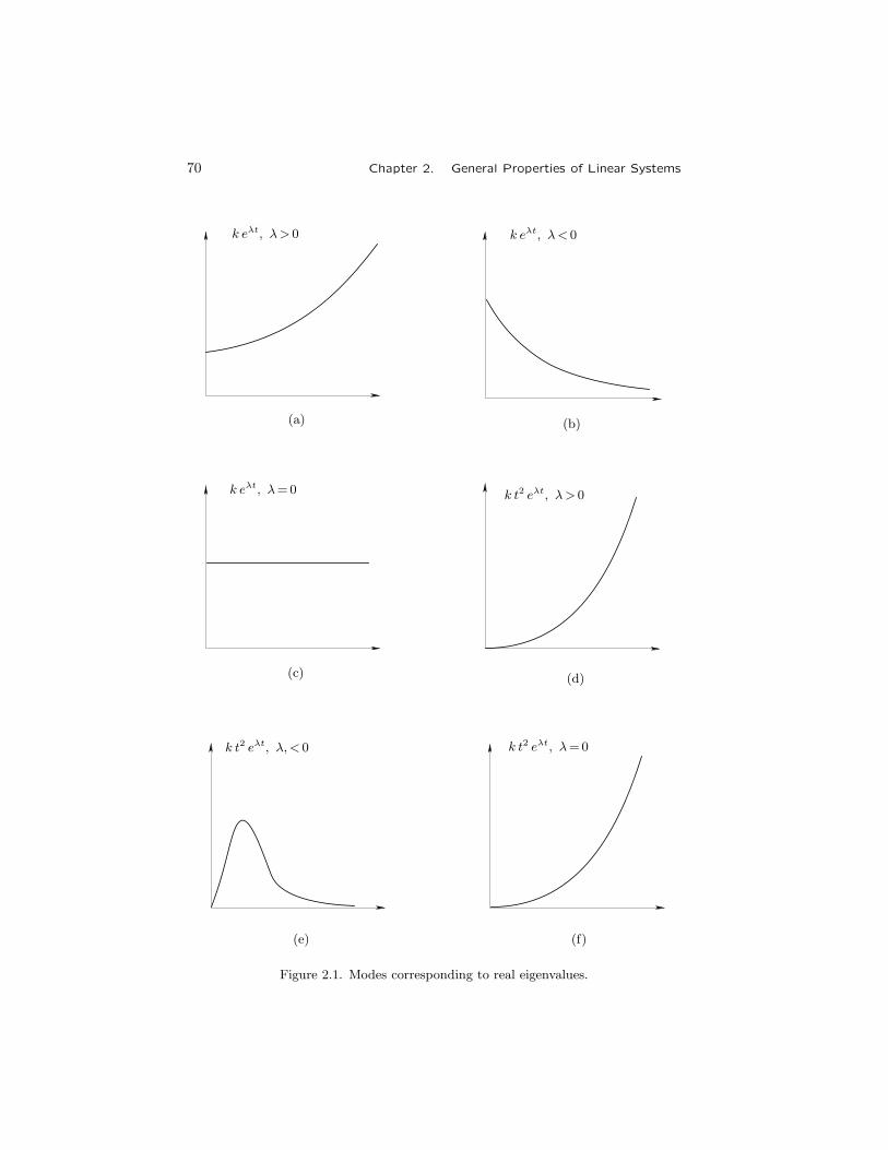
70 Chapter 2. General Properties of Linear Systems
k eλt, λ> 0 k eλt, λ< 0
k eλt, λ=0 k t2 eλt, λ> 0
k t2 eλt, λ,< 0 k t2 eλt, λ=0
(a) (b)
(c) (d)
(e) (f)
Figure 2.1. Modes corresponding to real eigenvalues.

2.1. The Free State Evolution of Linear Systems 71
k eλt + k∗ eλ∗ t, σ > 0 k eλt + k∗ eλ
∗ t, σ < 0
k eλt + k∗ eλ∗ t, σ=0 t2(k eλt + k∗ eλ
∗ t), σ > 0
t2(k eλt + k∗ eλ∗ t), σ < 0 t2(k eλt + k∗ eλ
∗ t), σ=0
(a) (b)
(c) (d)
(e) (f)
Figure 2.2. Modes corresponding to pairs of complex conjugate eigenvalues.

72 Chapter 2. General Properties of Linear Systems
and denote by u, v, and σ, ω the real and imaginary parts of h and λ respectively,so that
S = tr((u+ jv)e(σ+ jω)t + (u− jv)e(σ− jω)t
)By defining
m := 2 |h| , ϕ := arg h
it follows that
S =m
2tr eσt
(ej(ωt+ϕ) + e−j(ωt+ϕ)
)= mtr eσt cos(ωt+ ϕ)
= mtr eσt sin(ωt+ ϕ+
π
2
)When r is zero the resulting time function is typically one of those shown
in Fig. 2.2(a–c) (respectively for λ positive, negative, and zero), while for rdifferent from zero, for instance r=2, it is one of those shown in Fig. 2.2(d–f).
The same result could have been obtained by considering the “real” Jordanform whose general block is of the type (A.4.26): denote by σ, ω the real andimaginary part of λ and define
C :=
[σ ω−ω σ
](2.1.52)
so that
eC t =
[eσt cosωt eσt sinωt−eσt sinωt eσt cosωt
](2.1.53)
as can be checked by applying the identity
d
dteC t = C eC t
It is easily seen that the exponential of a “real” Jordan block of type (A.4.26)has the same structure as matrix (2.1.42), but with 2× 2 matrices eCit insteadof scalars eλit in the terms on and above the main diagonal, 2× 2 null matricesinstead of the scalar 0’s below the main diagonal.
It is now possible to draw some interesting conclusions: the general mode(2.1.47) corresponds to a function of time whose behavior as time approachesinfinity is one of the following:
1. It converges to zero if the real part of the corresponding eigenvalue isnegative;
2. It remains bounded if r is zero and the real part of the correspondingeigenvalue is zero;
3. It diverges if the real part of the corresponding eigenvalue is positive or ifr is different from zero and the real part of the eigenvalue is zero.
The above modes are called respectively asymptotically or strictly stable,(merely) stable and unstable.

2.1. The Free State Evolution of Linear Systems 73
2.1.5 Linear Time-Invariant Discrete Systems
All the previous arguments will be briefly extended to discrete-time systems.Consider the discrete-time constant homogeneous system
x(i + 1) = Ad x(i) (2.1.54)
whose state transition matrix is clearly
Φ(i, j) = Ai−jd (2.1.55)
i.e., reduces to the power of a matrix .The four procedures to compute the state transition matrix of continuous-
time systems can also be profitably used in the discrete-time case.
The Direct Method. Repeating the matrix multiplication many times mayinvolve significant errors due to truncation and great computation time. Tominimize these drawbacks, it is convenient to use the binary powering method :4
expand exponent k in binary form as
k =
n∑i=0
βi 2i
then initialize i← 0, Z←Ad, B← I if β0 =0 or B←Ad if β0 =1 and, untili=n, compute i← i+1, Z←Z2, B←B if βi=0 or B←ZB if βi=1. At theend, the result B=Ak
d is obtained. The coefficients βi (i=0, 1, . . . , n) can beobtained at each step as the remainders of repeated divisions of k by 2 in theset of integers, until the quotient is zero.
Use of the Jordan form. From
B = T−1Ad T
it follows that
Bk = T−1A kd T , hence A k
d = T Bk T−1
Consider (A.4.11). Clearly
Bk =
⎡⎢⎢⎢⎢⎢⎢⎢⎢⎣
Bk11 O . . . O . . . OO Bk
12 . . . O . . . O...
.... . .
.... . .
...O O . . . Bk
1,k1. . . 0
......
. . ....
. . ....
O O . . . O . . . Bkh,kh
⎤⎥⎥⎥⎥⎥⎥⎥⎥⎦
(2.1.56)
4 See Golub and Van Loan [B.3], p. 552.

74 Chapter 2. General Properties of Linear Systems
while the k-th power of a single �× � Jordan block is easily obtained by directcomputation as
Bkij =
⎡⎢⎢⎢⎢⎢⎢⎣
λki k λk− 1i
(k2
)λk− 2i . . .
(k
�−1)λk− �+1i
0 λki k λk− 1i . . .
(k
�−2)λk− �+2i
0 0 λki . . .(
k�−3
)λk− �+3i
......
.... . .
...0 0 0 . . . λki
⎤⎥⎥⎥⎥⎥⎥⎦
(2.1.57)
where (kh
):=
⎧⎪⎨⎪⎩k(k− 1) . . . (k− h+1)
h !for k ≥ h , h > 0
1 for k ≥ h , h = 00 for k < h
The Interpolating Polynomial Method. By means of the proceduredescribed in Subsection 2.1.3, the general element of the k-th power of matrixAd is obtained as (
A kd
)ij= 〈kij(Ad), v〉 (2.1.58)
where both kij(Ad) and v belong to Cm and m denotes the degree of theminimal polynomial of Ad . Vector v is defined as
v :=(λk1 , k λ
k− 11 , . . . , k(k− 1) . . . (k−m1 +2)λk−m1 +1
1 , . . . ,
λkh, k λk− 1h , . . . , k(k− 1) . . . (k−mh +2)λk−mh +1
h
)(2.1.59)
Relation (2.1.59) only makes sense when k≥m. However, the following equiv-alent expression for v holds without any constraint on the value of k.
v =(λk1 , k λ
k− 11 , 2!
(k2
)λk− 21 , . . . , (m1− 1)!
( k
m1− 1
)λk−m1 +11 , . . . ,
λkh, k λk− 1h , 2!
(k2
)λk− 2h , . . . , (mh− 1)!
( k
mh− 1
)λk−mh +1h
)(2.1.60)
Use of the Schur form. By means of a procedure similar to the onepresented for computation of the matrix exponential, it is possible to reduce thecomputation of A k
d to the solution of scalar difference equations of the generaltype
z(k + 1) = λi z(k) + b frj(k) , z(0) = 0 (2.1.61)
where
frj(k) = r!(kr
)λk−rj (j=1, . . . , h; r=0, . . . ,mj − 1) (2.1.62)
In the solution of (2.1.61) two cases are possible.
2.1. The Free State Evolution of Linear Systems 75
1. λi = λj . Solution of (2.1.61) is
z(k) =b
r+1(r+1)!
( k
r+1
)λk− r− 1i (2.1.63)
2. λi �=λj . In this case z(k) is computed by considering the sequence of func-tions w�(k) (�=0, . . . , r) defined below, which are the solutions of (2.1.61)with forcing terms f�j(k) (�=0, . . . , r). The solution is z(k)=wr(k), with
w0(k) = bλki − λkjλi − λj
w�(k) =1
λi − λj
(� w�−1(k)− b � !
(k�
)λk−�j
)(�=1, . . . , r)
(2.1.64)
Also in the case of discrete-time systems the components of vector v in(2.1.59) or (2.1.60) are called modes . Modes corresponding to a pair of complexconjugate eigenvalues appear with complex conjugate coefficients. The sum(2.1.51) in this case is changed into
S :=(kr
) (hλk− r + h ∗ λ∗ k− r
)(2.1.65)
or, by using the previously introduced notation
S =(kr
) ((u+ jv)(σ + jω)k− r + (u− jv)(σ − jω)k− r
)By setting
ρ := |λ| , ϑ := argλ
m := 2 |h| , ϕ := arg h
it follows that
S =m
2
(kr
)ρk
(ej((k− r)ϑ+ϕ) + e−j((k− r)ϑ+ϕ)
)
= m(kr
)ρk cos
((k− r)ϑ + ϕ
)
= m(kr
)ρk sin
((k− r)ϑ + ϕ+
π
2
)Furthermore, instead of (2.1.52, 2.1.53) the following matrices are easily derived
C =
[ρ cosϑ ρ sinϑ−ρ sinϑ ρ cosϑ
](2.1.66)

76 Chapter 2. General Properties of Linear Systems
Ck =
[ρk cos kϑ ρk sin kϑ−ρk sin kϑ ρk cos kϑ
](2.1.67)
The k-th power of a “real” Jordan block of type (A.4.26) has the same structureas matrix (2.1.57) but, on and above the main diagonal, functions λk− �+1
i arereplaced by 2× 2 matrices Ck− �+1
i and, below the main diagonal, zeros arereplaced by 2× 2 null matrices.
The general mode (2.1.62) has one of the following behaviors as k ap-proaches infinity:
1. It converges to zero if the magnitude of the corresponding eigenvalue is lessthan one;
2. It remains bounded if r is zero and the magnitude of the correspondingeigenvalue is equal to one;
3. It diverges if the magnitude of the corresponding eigenvalue is greater thanone or if r is different from zero and the magnitude of the eigenvalue isequal to one.
These modes are called respectively asymptotically or strictly stable,(merely) stable, and unstable.
2.2 The Forced State Evolution of Linear Sys-tems
Let us now examine specifically linear systems whose evolution in time isdescribed in Section 1.3 by equations (1.3.8, 1.3.9) in the continuous-time caseand (1.3.10, 1.3.11) in the discrete-time case. In order to derive solutions forthese equations, we will refer to the mathematical background presented in theprevious section, in particular to the concepts of the state transition matrixand the function of a matrix.
2.2.1 Linear Time-Varying Continuous Systems
First refer to differential equation (1.3.8) and denote by Φ(t, t0) the statetransition matrix of the related homogeneous equation
x(t) = A(t)x(t) (2.2.1)
An expression for the state transition function ϕ(t, t0, x0, u|[t0,t]) is derivedas follows.
Theorem 2.2.1 The solution of differential equation (1.3.8), with initial con-dition x(t0)= x0 and piecewise continuous input function u(·), is
x(t) = Φ(t, t0)x(t0) +
∫ t
t0
Φ(t, τ)B(τ)u(τ) dτ (2.2.2)

2.2. The Forced State Evolution of Linear Systems 77
Proof. First, clearly (2.2.2) satisfies the initial condition, since Φ(t0, t0)= I.Then by differentiating both members of (2.2.2) and taking into account therule for computation of the derivative of an integral depending on a parameter(see footnote 1 in Section 1.2) one obtains
x(t) = Φ(t, t0)x(t0) + Φ(t, t)B(t)u(t) +
∫ t
t0
Φ(t, τ)B(τ)u(τ) dτ
= A(t)
(Φ(t, t0)x0 +
∫ t
t0
Φ(t, τ)B(τ)u(τ) dτ
)+B(t)u(t)
= A(t)x(t) +B(t)u(t) �
Since Theorem 2.2.1 is of basic importance in linear system theory, wepresent another simple proof of it.
Another Proof of Theorem 2.2.1. For any identically nonsingular anddifferentiable matrix function of time X(t), consider the relation
d
dtX−1(t) = −X−1(t) X(t)X−1(t)
which is obtained by differentiating the identity X−1(t)X(t)= I. ReplacingX(t) with Φ(t, t0) yields
d
dt
(Φ−1(t, t0)x(t)
)= −Φ−1(t, t0) Φ(t, t0)Φ−1(t, t0)x(t) + Φ−1(t, t0) x(t)
From Φ(t, t0)=A(t)Φ(t, t0) and differential equation (1.3.8) it follows that
d
dt
(Φ−1(t, t0)x(t)
)= Φ−1(t, t0)
(x(t)−A(t)x(t)
)= Φ−1(t, t0)B(t)u(t)
By integrating both members, we finally obtain
Φ−1(t, t0)x(t) = c+
∫ t
t0
Φ−1(τ, t0)B(τ)u(τ) dτ
where c denotes a constant vector depending on the initial condition. Byusing inversion and composition properties of the state transition matrix, itis immediately shown that the above formula is equivalent to (2.2.2). �
Substitution of (2.2.2) into (1.3.9) immediately provides the following ex-pression for the response function γ(t, t0, x0, u|[t0,t]):
y(t) = C(t)Φ(t, t0)x0 + C(t)
∫ t
t0
Φ(t, τ)B(τ)u(τ) dτ +D(t)u(t)
= C(t)Φ(t, t0)x0 +
∫ t
t0
C(t)Φ(t, τ)B(τ)u(τ) dτ +D(t)u(t) (2.2.3)

78 Chapter 2. General Properties of Linear Systems
The integrals on the right of (2.2.2, 2.2.3) are convolution integrals whosekernels are the functions
V (t, τ) = Φ(t, τ)B(τ) (2.2.4)
W (t, τ) = C(t)Φ(t, τ)B(τ) +D(t) δ(t) (2.2.5)
Matrix W (t, τ) is called the impulse response of the system. The symbolδ(t) denotes a Dirac impulse which is introduced as follows. Consider thepiecewise continuous function Δ(τ, t0, ·) represented in Fig. 2.3 and supposethat parameter τ tends to zero: at the limit, we obtain having infinite amplitudeand unitary area. The Dirac impulse at t=0 will be denoted by δ(t) and att= t0 by δ(t− t0). Still referring to Fig. 2.3, we define∫ t2
t1
δ(t− t0) dt := limτ→0
∫ t2
t1
Δ(τ, t0, t) dt = 1
Δ(τ, t0, t)
1τ
0 t1 t0 t0 + τ t2 t
Figure 2.3. An impulse.
Similarly, for any continuous function of time f(·), we define∫ t2
t1
f(t) δ(t− t0) dt := limτ→0
∫ t2
t1
f(t)Δ(τ, t0, t) dt = f(t0)
Referring now to a purely dynamic system [D(t)=O in (1.3.9)] with zeroinitial state, apply the impulse represented in Fig. 2.3 to its i-th input, theother inputs being set equal to zero. At the limit for τ approaching zero weobtain
yi(t) =
∫ t
t0
W (t, τ) ei δ(t− t0) dτ =W (t, t0) ei (i=1, . . . , p)
where ei denotes the i-th column of the identity matrix Ip. Hence each singlecolumn of W (t, t0) represents the system response to a Dirac impulse appliedat t0 to each single input.
Relation (2.2.3) for a purely dynamic system with zero initial state becomes
y(t) =
∫ t
t0
W (t, τ)u(τ) dτ (2.2.6)

2.2. The Forced State Evolution of Linear Systems 79
This means that the zero-state response of a purely dynamic linear systemdepends only on its impulse response function. Equation (2.2.6) is a typicalinput-output model or IO model of a linear system, while equations (1.3.8, 1.3.9)represent an input-state-output model or ISO model .
2.2.2 Linear Time-Varying Discrete Systems
The previous considerations can easily be extended to the discrete-time case,corresponding to system equations (1.3.10, 1.3.11). Often discrete-time systemsderive from continuous ones subject to piecewise constant input functions of thetype shown in Fig. 1.8 and with output accordingly sampled. Denote by t0 + iT(i=0, 1, . . .) the times corresponding to input changes and output sampling.Matrices of the discrete-time model are related to those of the continuous-timeone by:
Ad(i ) = Φ(t0 +(i+1)T, t0+ iT
)(2.2.7)
Bd(i ) =
∫ t0+(i+1)T
t0+iT
Φ(t0 + (i+1)T, τ
)B(τ) dτ (2.2.8)
Cd(i ) = C(t0 + iT ) (2.2.9)
Dd(i ) = D(t0 + iT ) (2.2.10)
The state transition matrix Φ(i, j ) in this case is derived in connection withthe homogeneous difference equation
x(i + 1) = Ad(i )x(i ) (2.2.11)
The following theorem is the discrete counterpart of Theorem 2.2.1 and caneasily be proved by direct check.
Theorem 2.2.2 The solution of the difference equation (1.3.10) with initialcondition x(j )=x0 is
x(i ) = Φ(i, j )x0 +i−1∑k=j
Φ(i, k+1)Bd(k)u(k) (2.2.12)
Substitution of (2.2.12) into (1.3.10) yields
y(i ) = Cd(i )Φ(i, j )x0 + Cd(i )
i−1∑k=j
Φ(i, k+1)Bd(k)u(k) +
Dd(i )u(i ) (2.2.13)
The right side members of (2.2.12, 2.2.13) represent the state transition andresponse function of the discrete-time case, respectively. The matrix
W (i, j ) := Cd(i )Φ(i, j+1)Bd(j ) +Dd(i) (2.2.14)
is called the impulse response of the considered discrete-time system. Its mean-ing is analogous to the continuous-time case. Its k-th column represents thezero-state response to an input identically zero, except for the k-th component,which is equal to one at time j.

80 Chapter 2. General Properties of Linear Systems
2.2.3 Linear Time-Invariant Systems
The class of systems under consideration will now be further restricted to time-invariant ones which, in the continuous-time case, are described by
x(t) = Ax(t) +B u(t) (2.2.15)
y(t) = C x(t) +Du(t) (2.2.16)
and in the discrete-time case by
x(i + 1) = Ad x(i ) +Bd u(i ) (2.2.17)
y(i ) = Cd x(i ) +Dd u(i ) (2.2.18)
Time-invariance implies the following very important features:
1. A better computability of the state transition matrix and easier solvabilityof the nonhomogeneous differential equation which describes the state evolutionof the system subject to control. In fact, while in the time-varying case itis necessary to use numerical integration procedures (such as Runge-Kuttamethods), for time-invariant systems it is possible to express the state transitionmatrix in finite terms, for instance with the interpolating polynomial methodpresented in the previous section.
2. A more straightforward and deeper insight into the mathematical essenceof the structural constraints which may condition the action on the statethrough the input and/or the knowledge of the state through the output: suchan insight will be particularly stressed with the geometric techniques presentedin Chapters 3 and 4.
3. The possibility of relating state-space with polynomial matrix modelswhich, although very restricted in use (since they are not at all extensible tothe time-varying and nonlinear cases), allow a more satisfactory approach tosome structure-independent problems such as identification. This alternativemodeling of linear constant systems will be briefly reviewed in the next twosections.
In the continuous-time case the state transition function on the right of(2.2.2) is expressed in terms of the matrix exponential as follows:
x(t) = eAtx0 +
∫ t
0
eA(t− τ)B u(τ) dτ (2.2.19)
while in the discrete-time case the state transition function on the right of(2.2.12) is expressed in terms of the matrix power as
x(i ) = Adi x0 +
i−1∑j=0
Adi−j−1Bd u(j ) (2.2.20)
2.2. The Forced State Evolution of Linear Systems 81
Note that when dealing with time-invariant systems the initial time is usuallyassumed to be zero without any loss of generality because of the time-shiftingproperty. The two terms on the right of (2.2.19) and (2.2.20) represent thezero-input and zero-state transition function.
We now consider the computation of the right side member of (2.2.19).Thefirst term, i.e., the zero-input state transition function, is expressed in terms ofa simple matrix exponential, while a mathematical description of the inputfunction u(·) is needed to compute the second term, i.e., the convolutionintegral. Two important cases will be considered:
1. The input function is available as a sequence of samples;
2. The input function is available as a solution of a known homogeneous time-invariant differential equation.
Input Available as a Sequence of Samples. This case is easily trans-formed into a discrete-time case: denote by u(ti) (i=0, 1, . . . ) the input sam-ples and suppose that the actual input function is constant between samples,i.e., that u(t)=u(ti), ti≤ t< ti+1. This assumption is technically sound, sincein many cases input to a continuous-time system is provided by a digital pro-cessor with a “hold” output circuitry. In other cases, it is possible to use adiscretization fine enough to have good reproduction of the actual input, with-out any other approximation in solving the system differential equation. Inorder to improve the computational precision, it is also possible to introduce alinear interpolation between samples by means of an artifice, as will be shownin Subsection 2.2.5.
Consider a general instant of time t and denote by ti, ti+1 two subsequentsampling instants such that ti≤ t< ti+1; equation (2.2.19) can be written as
x(t) = eAtx0 +i−1∑k=0
(∫ tk+1
tk
eA(t−τ)dτ)B u(tk) +
(∫ t
ti
eA(t−τ)dτ)B u(ti)
= eAtx0 +
i−1∑k=0
eA(t−tk+1)f(A, (tk+1− tk)
)B u(tk) +
f(A, t)B u(ti) (2.2.21)
where f(A, t) denotes the matrix exponential integral, defined as
f(A, t) :=
∫ t
0
eAτdτ (2.2.22)
whose computation will be considered in the next subsection. In the previousderivation the following identity has been used:
∫ t1
t0
eA(t1−τ)dτ = −∫ 0
t1−t0eAxdx =
∫ t1−t0
0
eAτdτ
82 Chapter 2. General Properties of Linear Systems
In conclusion, the state transition function of a constant continuous-timesystem with a piecewise constant input is expressed as a finite sum whoseterms are easily computable using the matrix exponential and the matrixexponential integral. If sampling is uniform with period T and the output isalso synchronously sampled, the system is described by the discrete-time model(2.2.17, 2.2.18) where matrices Ad, Bd, Cd, Dd are related to the correspondingones of the continuous-time case by the relations
Ad := eAT (2.2.23)
Bd := f(A, T )B (2.2.24)
Cd := C (2.2.25)
Dd := D (2.2.26)
which particularize (2.2.7–2.2.10). In (2.2.24), f(A, T ) still denotes the functiondefined by (2.2.22). In conclusion, the computation is performed by using(2.2.20), which only requires a computational algorithm for the power of amatrix.
Input Provided by an Exosystem. We shall now consider the otherremarkable case in which the convolution integral in (2.2.19) is easily com-putable. The input is assumed to be a linear function of the solution of ahomogeneous linear differential equation, i.e., to be provided as the output ofthe time-invariant free system
v(t) = W v(t) , v(0) = v0 (2.2.27)
u(t) = L v(t) (2.2.28)
where W and L denote properly dimensioned real matrices. In explicit form,we have
u(t) = L eWt v0 (2.2.29)
This case has considerable practical importance: in fact, it allows the repro-duction of “test signals” such as steps, ramps, sine and cosine functions, whichare widely used for comparison and classification of dynamic system features.Since input in this case is a linear combination of modes, in order to distinguishthe outside modes from those inherent in the system itself, we will call the for-mer exogenous modes and the latter internal modes . System (2.2.27, 2.2.28),which generates exogenous modes, is called an exosystem. Design techniquesbased on using simple test signals as inputs, which are very easily manipulablein computations, are widely used in regulator synthesis.
Referring to the connection shown in Fig. 2.4, we introduce the extendedstate
x :=
[xv
]with x0 :=
[x0v0
]and the corresponding extended matrices
A :=
[A BLO W
], C := [C DL ]

2.2. The Forced State Evolution of Linear Systems 83
v0 x0
y
system
u
exosystem
v = W v
u = Lv
x = Ax+B u
y = C x+Du
Figure 2.4. A system connected to an exosystem.
The time evolution of the extended state and, in particular, of the system statethat is a part of it, is obtained as the solution of the homogeneous linear matrixdifferential equation
˙x(t) = A x(t) , x(0) = x0 (2.2.30)
Thusx(t) = eAt x0
and, consequently
y(t) = C x(t) = C eAt x0
i.e., the response function is determined by means of a matrix exponentialcomputation.
To show how this technique is used, let us report some examples. Considerthe single input system
x(t) = Ax(t) + b u(t) (2.2.31)
y(t) = C x(t) + d u(t) (2.2.32)
where b and d denote row matrices, and set the problem to determine its zero-state responses to the test signals shown in Fig. 2.5.
The signal shown in Fig. 2.5(a) is called a unit step: the zero-state responseof system (2.2.32, 2.2.32) to it is determined by extending the state with a scalarextra state coordinate v and considering the time evolution of the free system
˙x(t) = Ax(t) , x(0) = x0 (2.2.33)
y(t) = C x(t) (2.2.34)
where
A :=
[A bO 0
], x0 :=
[O1
], C := [C d ]
A similar procedure can be applied for the signal shown in Fig. 2.5(b), calleda unit ramp, for that shown in Fig. 2.5(c), consisting of the sum of a step anda ramp, and for the sinusoid shown in Fig. 2.5(d). In these cases two scalarextra state coordinates v1 and v2 are needed and matrices in (2.2.33, 2.2.34)are defined as
A :=
⎡⎣A b OO 0 1O 0 0
⎤⎦ , x0 :=
⎡⎣O01
⎤⎦ , C := [C d 0 ]

84 Chapter 2. General Properties of Linear Systems
uu
uu
t
t
tt
1
1
1
1
1
0
0
00
−1
k1
k2
u(t) =
{0 for t < 01 for t ≥ 0
u(t) =
{0 for t < 0t for t ≥ 0
u(t) =
{0 for t < 0k1 + k2 t for t ≥ 0
u(t) =
{0 for t < 0sin ω t for t ≥ 0
(a) (b)
(c) (d)
Figure 2.5. Some test signals.
A :=
⎡⎣A b OO 0 1O 0 0
⎤⎦ , x0 :=
⎡⎣ Ok1k2
⎤⎦ , C := [C d 0 ]
A :=
⎡⎣A b OO 0 ωO −ω 0
⎤⎦ , x0 :=
⎡⎣O01
⎤⎦ , C := [C d 0 ]
2.2.4 Computation of the Matrix Exponential Integral
Consider the matrix exponential integral, i.e., function f(A, t) defined by(2.2.22), which is used in expression (2.2.14) for the input distribution ma-trix of the discrete system corresponding to a uniformly sampled continuoussystem. If A is nonsingular, it can easily be expressed in terms of the matrix

2.2. The Forced State Evolution of Linear Systems 85
exponential by means of the relation
f(A, t) = A−1(eAt − I
)(2.2.35)
which follows from the term-by-term integration of the infinite series
eAt = I +At+A2t2
2+ . . .+
Aiti
i!+ . . . (2.2.36)
which yields
f(A, t) = It+At2
2+A2t3
6+ . . .+
Aiti+1
(i+1)!+ . . . (2.2.37)
clearly equivalent to (2.2.35). If A is singular, it is possible to use one of thefollowing two computational methods.
The Interpolating Polynomial Method. Consider the finite sum
f(A, t) =m−1∑i=0
ηi(t)Ai (2.2.38)
Define
w(t) :=(∫ t
0
eλ1τdτ ,
∫ t
0
τ eλ1τdτ , . . . ,
∫ t
0
τm1 − 1 eλ1τdτ , . . . ,∫ t
0
eλhτdτ ,
∫ t
0
τ eλhτdτ , . . . ,
∫ t
0
τmh − 1 eλhτdτ)
(2.2.39)
and compute the vector η(t)∈Rm having coefficients ηi(t) (i=0, . . . ,m− 1) ascomponents, by means of the relation
η(t) = V −1 w(t) (2.2.40)
where V is the same nonsingular matrix introduced in Subsection 2.1.3 tocompute a general function of a matrix. The components of vector w(t) areintegrals of the general type
Ik(t) :=
∫ t
0
τk eλτ dτ (2.2.41)
which, if λ �=0, can be computed by means of the recursion formula
Ik(t) =τk eλτ
λ
∣∣∣∣τ=t
τ=0
− k
λIk−1(t) (2.2.42)
This immediately follows from the well-known integration by parts∫ t1
t0
f(τ) g(τ) dτ = f(τ) g(τ)
∣∣∣∣τ=t1
τ=t0
−∫ t1
t0
f(τ) g(τ) dτ

86 Chapter 2. General Properties of Linear Systems
with the assumptions
f(τ) := τk hence f(τ) = k τk−1
g(τ) dτ := eλτ dτ hence g(τ) =1
λeλτ
On the other hand, for λ=0 it is possible to obtain directly
Ik(t) =tk+1
k + 1
Summing up:
Ik(t) =
⎧⎪⎪⎪⎪⎪⎨⎪⎪⎪⎪⎪⎩
eλt
λ
(tk − k
λtk−1 +
k(k− 1)λ2
tk−2−
. . . + (−1)k k!λk
)− (−1)k k!
λk+1 for λ �=0
tk+1
k + 1for λ=0
(2.2.43)
v0 x0
x
system
u
integrators
v = 0
u = vx = Ax+B u
Figure 2.6. Representation of extended system (2.2.44, 2.2.45).
A Submatrix of an Extended Matrix Exponential. Function f(A, t)can be computed also as a submatrix of the matrix exponential of a properlyextended system. We shall present this method for the direct computation ofmatrix Bd defined in (2.2.24): of course, it will provide f(A, t) in the particularcase Bd := In. Consider the continuous-time extended free system
˙x(t) = A x(t) , x(0) = x0 (2.2.44)
with
x :=
[xv
], x0 :=
[x0v0
], A :=
[A BO O
](2.2.45)
which represents the interconnection shown in Fig. 2.6. Clearly v(t)= v0 in thetime interval [0, T ] for any T , so that, from
x(T ) = eAT x0 =
[eATx0 + f(A, T )Bv0
v0
]it follows that
eAT =
[eAT f(A, T )BO Ip
]=
[Ad Bd
O Ip
](2.2.46)
i.e., Ad, Bd are easily derived as submatrices of the above extended matrixexponential.

2.2. The Forced State Evolution of Linear Systems 87
2.2.5 Approximating Continuous with Discrete
Discretizing the input function was presented in Subsection 2.2.3 as a methodto compute the convolution integral on the right of (2.2.19): the input was ap-proximated with a piecewise constant function, so that the convolution integralwas transformed into a finite sum with terms easily computable as functions ofthe “matrix exponential” and “matrix exponential integral” types.
uu
uu
00
00
jj
jj
j+1j+1
j+1j+1
ii
ii
tt
tt
(a) (b)
(c) (d)
Figure 2.7. Several ways to reconstruct a continuous function from samples.
Such a reconstruction of a continuous function from a finite sequence ofsamples is not unique: other means to reach the same goal are representedin Fig. 2.7. Two of them, those shown in Fig. 2.7(a) and Fig. 2.7(d), canalso be used to convert, in real time, a sequence of samples into a functionof time, so that they correspond to actual hold devices , while those shown inFig. 2.7(b) and Fig. 2.7(c) cannot be implemented in real time since they requireknowledge of the next sample at any instant of time; nevertheless, they can beused to compute the convolution integral, because in this case the sequence ofall samples can be assumed to be a priori known.
The four approximations are called, respectively: backward rectangular orzero-order hold , forward rectangular , trapezoidal , and first-order hold . The
88 Chapter 2. General Properties of Linear Systems
first-order hold approximation consists of maintaining between the sample atiT and that at (i+1)T , the constant slope corresponding to linear interpolationbetween samples at (i− 1)T and iT .
Recall definitions (2.2.23, 2.2.24) for Ad, Bd: the convolution integral inbackward rectangular and forward rectangular approximations is computed byexpressing the effect at time k of the pulse at generic time j (emphasized byhatching in figure) and summing over j. The following expressions are obtainedin the two cases:
k−1∑j=0
Ak−j−1d Bd u(j ) (2.2.47)
k−1∑j=0
Ak−j−1d Bd u(j+1) (2.2.48)
In the cases of trapezoidal and first-order hold approximations, the genericimpulse is trapezoidal instead of rectangular and can be expressed as the sum ofa rectangle and a triangle. The effect of the triangular pulse can be computedby means of an artifice, by considering that the triangular pulse with amplitudeΔu can be obtained from an auxiliary dynamic system that integrates over Ta rectangular pulse with amplitude Δu/T with zero initial condition. Considerthe extended system[
x(t)z(t)
]=
[A BO O
] [x(t)z(t)
]+
[OIp
]u(t)
which, in fact, represents the original system with an integrator on each input.Denote by A1 and B1 the corresponding matrices and set
C1 := [ In O ]
The effect at time T of a triangular pulse with amplitude Δu applied between0 and T is
1
TC1 f(A1, T )B1Δu
Let
Bt :=1
TC1 f(A1, T )B1
The convolution integral is approximated in the two cases by the sums
k−1∑j=0
Ak−j−1d
(Bd u(j ) +Bt
(u(j+1)− u(j )
))(2.2.49)
k−1∑j=0
Ak−j−1d
(Bd u(j ) +Bt
(u(j )− u(j− 1)
)), u(−1) := 0 (2.2.50)

2.3. IO Representations of Linear Constant Systems 89
Matrices Ad, Bd, Bt can be computed as submatrices of the exponential of aproperly extended matrix. In fact, it is easily shown that
eAT =
⎡⎣Ad Bd T Bt
O Ip T IpO O Ip
⎤⎦ if A :=
⎡⎣A B OO O IpO O O
⎤⎦ (2.2.51)
2.3 IO Representations of Linear Constant Sys-
tems
Consider a time-invariant continuous-time linear system Σ with input u∈Rp
and output y∈Rq. A typical input-output representation (or briefly IO repre-sentation) of Σ is a differential equation of the type5
μ∑k=0
Qkdk
dtky(t) =
μ∑k=0
Pkdk
dtku(t) (2.3.1)
where Pk and Qk (k=1, . . . , μ) denote real matrices with dimensions q× p andq× q respectively; in particular, Qμ is assumed to be nonsingular. The integerμ is called the order of the representation.
For a simpler notation and more straightforward algebraic handling, it iscustomary to represent with a polynomial any differential operator consistingof a linear combination of the derivatives of a given time function, like bothmembers of (2.3.1). Let, for any function of time6 c(·):
s x(t) :=d
dtx(t) , s2 x(t) :=
d2
dt2x(t) , . . .
and, accordingly, write (2.3.1) as
μ∑k=0
Qk sk y(t) =
μ∑k=0
Pk sk u(t)
or simplyQ(s) y(t) = P (s)u(t) (2.3.2)
5 The differential equation (2.3.1) has a meaning only if input and output functions aredifferentiable at least μ times. This assumption is very restrictive in system theory, whereit is often necessary to refer to piecewise continuous functions, which are not differentiable,at least at discontinuity points. For a rigorous approach (2.3.1) should be interpreted in thelight of distribution theory, i.e., in the framework of a suitable extension of the concept offunction. This is not at all worth doing for the particular case at hand, since the drawbackcan be overcome in a simple and realistic way by considering (2.3.1) merely as a conventionalrepresentation of the integral equation obtained by integrating both its members μ times,and introducing each time in one of its members a proper integration constant whose valueis related to the system initial condition.
6 It is worth noting at this point that the introduction of the Laplace transform andrelated mathematical background is very far beyond the scope of this book; here symbol sand polynomials in s are simply short notations for the linear operator “first derivative” anda linear combination of a function and its subsequent order derivatives.

90 Chapter 2. General Properties of Linear Systems
where P (s) and Q(s) denote polynomial matrices defined by
P (s) :=
μ∑k=0
Pk sk , Q(s) :=
μ∑k=0
Qk sk (2.3.3)
The discrete-time case can be handled in a very similar way. Considera time-invariant discrete-time linear system Σ with input u∈Rp and outputy ∈Rq. A typical input-output representation of Σ is a difference equation ofthe type
μ∑k=0
Qk y(i + k) =
μ∑k=0
Pk u(i+ k) (2.3.4)
where Pk and Qk (k=1, . . . , μ) denote real matrices with dimensions q× p andq× q respectively; in particular, Qμ is assumed to be nonsingular. The integerμ is called the order of the representation. For a simpler notation, referring toany sequence x(i ) (i=1, 2, . . . ) define
z x(i ) := x(i + 1) , z2 x(i ) := x(i + 2) , . . .
and write (2.3.4) accordingly as
Q(z) y(i ) = P (z)x(i ) (2.3.5)
where P (z) and Q(z) are the polynomial matrices
P (z) :=
μ∑k=0
Pk zk , Q(z) :=
μ∑k=0
Qk zk (2.3.6)
In the cases of single-input single-output systems, i.e., when p= q=1,equations (2.3.2) and (2.3.5), referring respectively to the continuous- and thediscrete-time cases, can be written simply as
y(t) =P (s)
Q(s)u(t) , y(i ) =
P (z)
Q(z)u(i )
In this way the product of a time function or a time sequence by a ratio ofpolynomials in the variable s (the derivative operator) or z (the shift operator)is given a well-defined conventional meaning. Such ratios are called transferfunctions of the systems referred to and are a complete representation of theirzero-state dynamic behavior; their usefulness is particularly clear in dealingwith complex systems consisting of numerous interconnected parts. In fact,the rules for the reduction of block diagrams and signal-flow graphs, which arebriefly presented as complementary material of this chapter, can be appliedto transfer functions as well as to real transmittance coefficients, and lead tooverall transfer functions which in the previous convention represent the ac-tual differential or difference equation relating the particular input and output
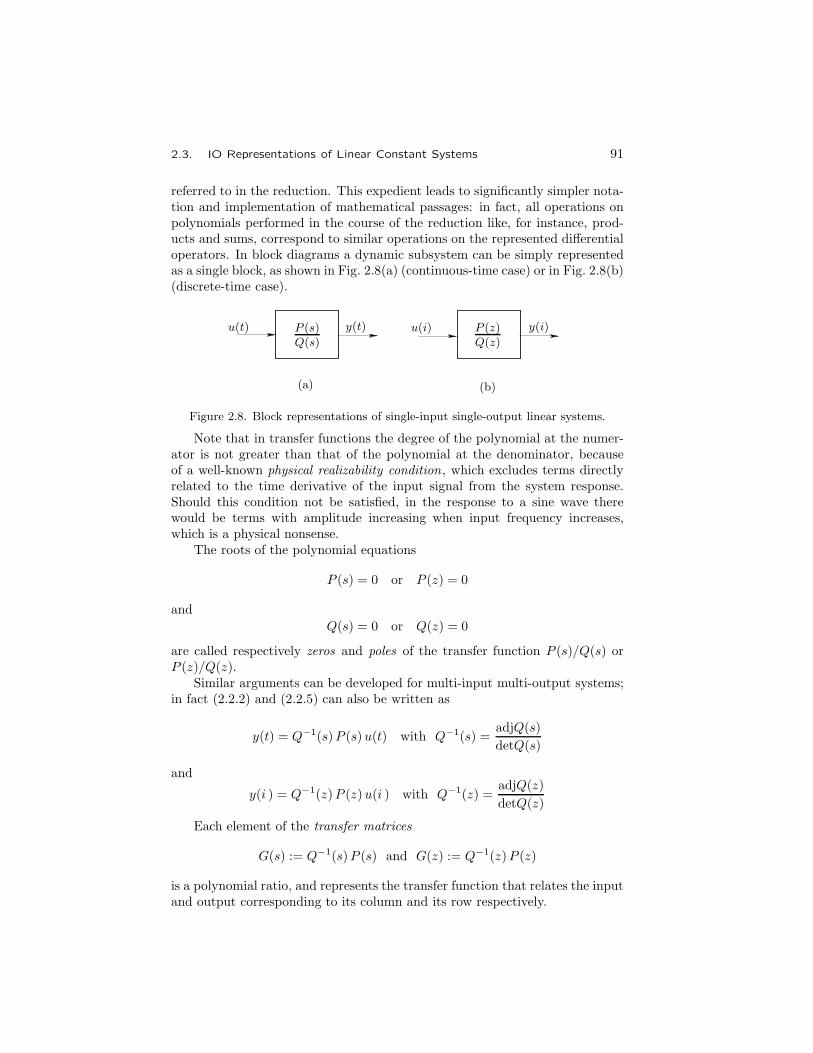
2.3. IO Representations of Linear Constant Systems 91
referred to in the reduction. This expedient leads to significantly simpler nota-tion and implementation of mathematical passages: in fact, all operations onpolynomials performed in the course of the reduction like, for instance, prod-ucts and sums, correspond to similar operations on the represented differentialoperators. In block diagrams a dynamic subsystem can be simply representedas a single block, as shown in Fig. 2.8(a) (continuous-time case) or in Fig. 2.8(b)(discrete-time case).
u(t) P (s)Q(s)
y(t) P (z)Q(z)
u(i) y(i)
(a) (b)
Figure 2.8. Block representations of single-input single-output linear systems.
Note that in transfer functions the degree of the polynomial at the numer-ator is not greater than that of the polynomial at the denominator, becauseof a well-known physical realizability condition, which excludes terms directlyrelated to the time derivative of the input signal from the system response.Should this condition not be satisfied, in the response to a sine wave therewould be terms with amplitude increasing when input frequency increases,which is a physical nonsense.
The roots of the polynomial equations
P (s) = 0 or P (z) = 0
and
Q(s) = 0 or Q(z) = 0
are called respectively zeros and poles of the transfer function P (s)/Q(s) orP (z)/Q(z).
Similar arguments can be developed for multi-input multi-output systems;in fact (2.2.2) and (2.2.5) can also be written as
y(t) = Q−1(s)P (s)u(t) with Q−1(s) =adjQ(s)
detQ(s)
and
y(i ) = Q−1(z)P (z)u(i ) with Q−1(z) =adjQ(z)
detQ(z)
Each element of the transfer matrices
G(s) := Q−1(s)P (s) and G(z) := Q−1(z)P (z)
is a polynomial ratio, and represents the transfer function that relates the inputand output corresponding to its column and its row respectively.

92 Chapter 2. General Properties of Linear Systems
In the multivariable case poles are the roots of the polynomial equationsdetQ(s)= 0 or detQ(z)= 0, while the extension of the concept of zero leadsto the so-called invariant zeros , which will be defined in Section 4.4 in theframework of the geometric approach.
2.4 Relations Between IO and ISO Representa-tions
It is quite evident that the IO (input-output) and the ISO (input-state-output)representations of linear dynamic constant systems are equivalent and relatedto each other. This section considers the problem of deriving any one of themfrom the other.
The IO description appears to be more compact and more direct, partic-ularly when a mathematical model of a real system is derived from records ofthe input and output functions by means of an identification procedure; how-ever, in engineering practice the state-space approach is more convenient forthe following reasons:
1. the relative ease with which some nonlinearities and physical bounds, suchas saturations, are taken into account;
2. a more direct dependence of the model coefficients on the actual values ofphysical parameters, which facilitates the study of sensitivity and robustness.
These reasons are important enough to adopt the ISO representation andrestrict the IO one to the domain of mathematical inquisitiveness, providedthe widespread belief that IO models are necessary to solve such problems asregulation, noninteraction, and stabilization, is absolutely unfounded. In fact,in this book such problems will be solved referring exclusively to ISO models:the passage from one to the other of the representations will be considered inthis section, merely as an interesting exercise.
We will consider first the passage from ISO to IO representation, for whicha constructive procedure is suggested in the proof of the following theorem.
Theorem 2.4.1 System (2.2.15, 2.2.16) admits an IO representation of thetype (2.3.2, 2.3.3), in which μ is the degree of the minimal polynomial of A.
Proof. Consider the subsequent time derivatives of both members of (2.2.16)and take into account (2.2.15):
y(t) = C x(t) +Du(t)
s y(t) = C Ax(t) + C B u(t) +D su(t)
s2 y(t) = C A2 x(t) + C AB u(t) + C B su(t) +D s2 u(t)
. . . . . . . . .
sμ y(t) = C Aμ x(t) +
μ−1∑j=0
C Aj B sμ−j−1 u(t) +D sμ u(t)
2.4. Relations Between IO and ISO Representations 93
Let λμ + q1λμ− 1 + . . . + qμ be the minimal polynomial of A. Multiply the
first of the above relations by qμ, the second by qμ− 1, and so on, so that thelast but one is multiplied by q1, and sum all of them. It follows that
sμ y(t) +
μ∑i=1
qi sμ−i y(t) =
μ∑i=1
Pi si u(t) (2.4.1)
where Pi (i=1, . . . , μ) are constant q× pmatrices. The obtained representationis clearly of the type (2.3.2, 2.3.2). �
The following similar result for discrete-time systems is derived by simplyreplacing s with z.
Corollary 2.4.1 System (2.2.17, 2.2.18) admits an IO representation of thetype (2.3.5, 2.3.6), in which μ is the degree of the minimal polynomial of Ad.
From (2.4.1) the transfer matrix G(s) is immediately derived. Collectingy(t) on the left and dividing by the minimal polynomial yields
G(s) =
∑μi=0 Pi s
i
sμ +∑μ
i=1 qi sμ−i (2.4.2)
Note that every element of the matrix on the right of (2.4.2) is a strictly properrational function.
Another procedure to derive the system transfer matrix is the following.Write (2.2.15, 2.2.16) in the form
s x(t) = Ax(t) +B u(t)
y(t) = C x(t) +Du(t)
Thus
x(t) = (sI − A)−1B u(t)y(t) =
(C (sI −A)−1B +D
)u(t)
hence
G(s) = C (sI −A)−1 B +D
=1
det(sI −A) C adj(sI −A)B +D (2.4.3)
The rational functions in matrix (2.4.3) are strictly proper, sincedet(sI −A) is a polynomial with degree n and C adj(sI −A)B is a polynomialmatrix whose elements have degrees less than or equal to n− 1. The possibledifference between the maximal degree of the polynomial at the denominatorof (2.4.2) and that of (2.4.3) is due to possible cancellations of common factorsin numerator and denominator of polynomial fractions, which have not beenconsidered in deriving (2.4.3).

94 Chapter 2. General Properties of Linear Systems
2.4.1 The Realization Problem
We now consider the inverse problem, i.e., the passage from IO to ISO rep-resentation. In literature this is called the realization problem. Given thepolynomial matrices P (s), Q(s) which appear in (2.3.2) or transfer matrixG(s)=Q−1(s)P (s), derive matrices A,B,C,D of a corresponding ISO repre-sentation of type (2.2.15, 2.2.16). The solution to the realization problem isnot unique: even the state-space dimension n may be different in different re-alizations of the same transfer matrix. A minimal realization is one in whichn is a minimum. In this section we present a constructive procedure to derivea convenient realization, but not a minimal one, at least in the multi-inputmulti-output case.
First refer to a single-input single-output (SISO) system with transferfunction G(s), which is assumed to be proper rational of the type
G(s) =P (s)
Q(s)= k0 +
M(s)
Q(s)(2.4.4)
where M(s)/Q(s) is strictly proper. Denote by m the degree of P (s) and byn that of Q(s), which is assumed to be monic without any loss of generality:if not, divide both numerator and denominator by the coefficient of its greaterpower in s. If m<n, set k0 := 0, M(s) :=P (s); if m=n, divide P (s) by Q(s)and set k0 equal to the quotient and M(s) to the remainder. Furthermore,denote by λi, mi (i=1, . . . , h) the roots of the polynomial equation Q(s)= 0and their multiplicities.
It is well known that the strictly proper function M(s)/Q(s) admits thepartial fraction expansion
M(s)
Q(s)=
h∑i=1
mi∑�=1
ki�(s− λi)�
where
ki� :=1
(mi − �)!dmi − �
dsmi − �
((s− λi)mi
M(s)
Q(s)
)∣∣∣∣s=λi
(i = 1, . . . , h; � = 1, . . . ,mi) (2.4.5)
so that the transfer function can be written as
G(s) = k0 +
h∑i=1
mi∑�=1
ki�(s− λi)�
(2.4.6)
It is convenient to transform (2.4.6) into a form with real coefficients:suppose that λ1, . . . , λr are real and λr+1, . . . , λc are complex poles with theimaginary part positive, and λc+1, . . . , λh are their conjugates. Denote with

2.4. Relations Between IO and ISO Representations 95
σi, ωi the real and imaginary part of λi (i= r+1, . . . , c), with ui�, vi� the realand imaginary part of ki� (i= r+1, . . . , c; �=1, . . . ,mi), i.e.,
λi =
{σi + j ωi (i = r+1, . . . , c)σi − j ωi (i = c+1, . . . , h)
ki� =
{ui� + j vi� (i = r+1, . . . , c; �=1, . . . ,mi)ui� − j vi� (i = c+1, . . . , h; �=1, . . . ,mi)
The equivalence of (2.4.6) to the real coefficients expression
G(s) = k0 +
r∑i=1
mi∑�=1
ki�(s− λi)�
+
c∑i= r+1
mi∑�=1
αi� s+ βi�(s2 − ai s+ bi)�
(2.4.7)
whereai := 2 σibi := σi
2 + ωi2 (2.4.8)
and αi�, βi� are functions of σi, ωi, uik, vik (k=1, . . . , �), can be proved bydirect check.
1
1
1
1
1
1
s−1s−1
s−1s−1
σ + j ωσ + j ω
σ − j ωσ − j ω
u1 + j v1 u2 + j v2
z1 + j i1 z2 + j i2
u2 − j v2
z1 − j i1z2 − j i2
u1 − j v1
Figure 2.9. The Jordan-type complex realization.
Example 2.4.1 Consider the expansion (2.4.6) and, in particular, supposethat a double complex pole is present in it with its conjugate, and refer to thecorresponding terms
u1 + jv1s− σ − jω +
u2 + jv2(s− σ − jω)2 +
u1 − jv1s− σ + jω
+u2 − jv2
(s− σ + jω)2(2.4.9)
A signal-flow graph realization for these is shown in Fig. 2.9. It representsthe Jordan realization in the complex field. Note that the involved signalsz1 + ji1, z2 + ji2, z1− ji1, z2− ji2, are complex conjugate.
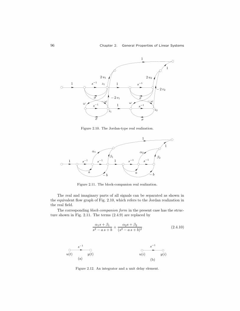
96 Chapter 2. General Properties of Linear Systems
1
1
1
1
1
s−1s−1
s−1s−1
σσ
σσ
2 u1 2u2
− 2 v2
i1 i2
− 2 v1
ωω−ω−ω
z1
Figure 2.10. The Jordan-type real realization.
1
1
11 s−1s−1s−1s−1
aa − b− b
α1 α2
β2β1
Figure 2.11. The block-companion real realization.
The real and imaginary parts of all signals can be separated as shown inthe equivalent flow graph of Fig. 2.10, which refers to the Jordan realization inthe real field.
The corresponding block-companion form in the present case has the struc-ture shown in Fig. 2.11. The terms (2.4.9) are replaced by
α1s+ β1s2 − a s+ b
+α2s+ β2
(s2 − a s+ b)2(2.4.10)
u(t)
s−1s−1
y(t) u(i) y(i)(a) (b)
Figure 2.12. An integrator and a unit delay element.

2.4. Relations Between IO and ISO Representations 97
chains of modes relating to λ1
chains of modes relating to λr
chains of modes relating to λr+1, λc+1
chains of modes relating to λc, λh
k0
u y
1
1
1
1
1
1
1
1
Figure 2.13. The general signal-flow graph for the single-input single-output case.
wherea = 2 σ , b = σ2 + ω2
α1 = 2 u1 , β1 = −2 u1 σ − 2 v1 ω + 2 u2
α2 = −4 v2 ω , β2 = −4 u2 ω2 + 4 v2 σ ω
The aforementioned identities can be derived by means of the followinggeneral procedure:
1. Express as a single fraction each pair of complex conjugate terms of theoriginal expansion;
2. Reduce the degree of the polynomial to one at the numerator of each termby means of repeated divisions: for instance, when the denominator is squared,use
N(s)
D2(s)=Q(s)
D(s)+
R(s)
D2(s)
where Q(s) and R(s) denote the quotient and the remainder of the division ofN(s) by D(s);
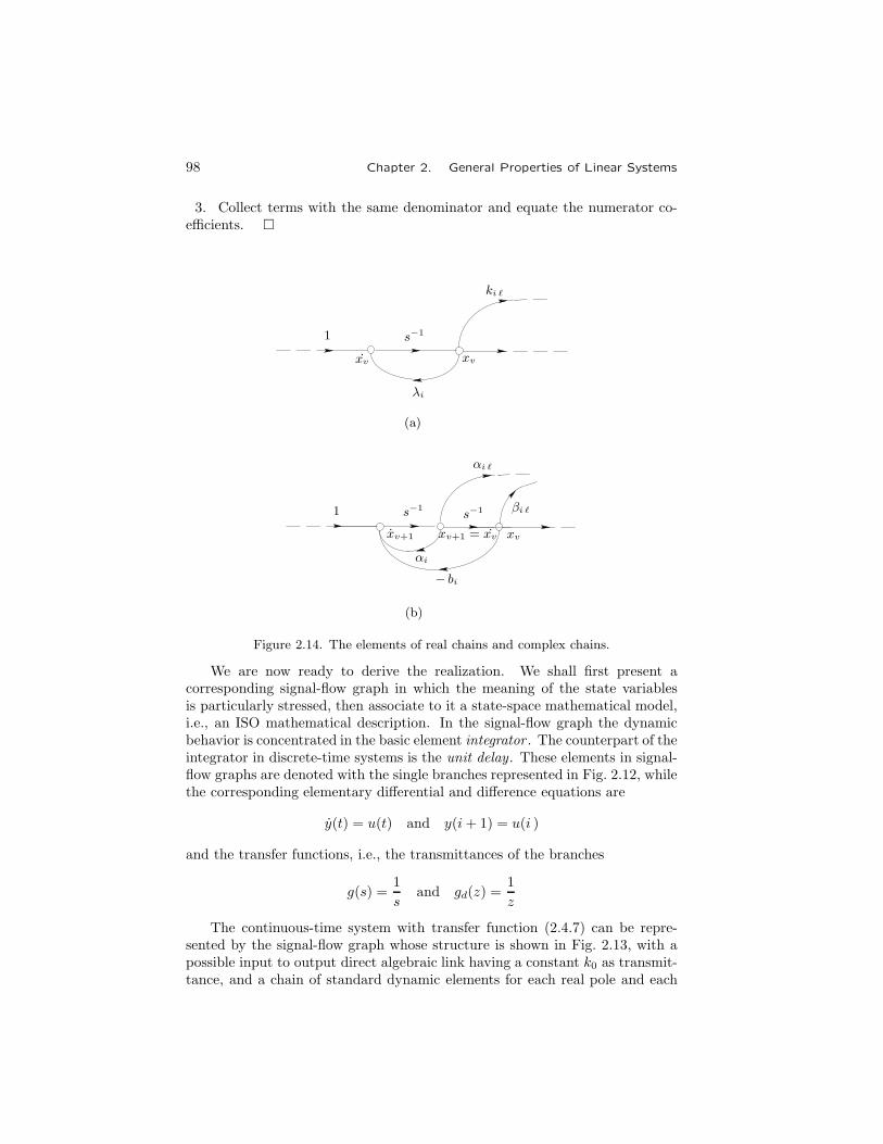
98 Chapter 2. General Properties of Linear Systems
3. Collect terms with the same denominator and equate the numerator co-efficients. �
1
1
s−1s−1
s−1
xv
xv
xv
λi
ki �
βi �
xv+1 xv+1 = xv
αi
− bi
αi �
(a)
(b)
Figure 2.14. The elements of real chains and complex chains.
We are now ready to derive the realization. We shall first present acorresponding signal-flow graph in which the meaning of the state variablesis particularly stressed, then associate to it a state-space mathematical model,i.e., an ISO mathematical description. In the signal-flow graph the dynamicbehavior is concentrated in the basic element integrator . The counterpart of theintegrator in discrete-time systems is the unit delay. These elements in signal-flow graphs are denoted with the single branches represented in Fig. 2.12, whilethe corresponding elementary differential and difference equations are
y(t) = u(t) and y(i+ 1) = u(i )
and the transfer functions, i.e., the transmittances of the branches
g(s) =1
sand gd(z) =
1
z
The continuous-time system with transfer function (2.4.7) can be repre-sented by the signal-flow graph whose structure is shown in Fig. 2.13, with apossible input to output direct algebraic link having a constant k0 as transmit-tance, and a chain of standard dynamic elements for each real pole and each
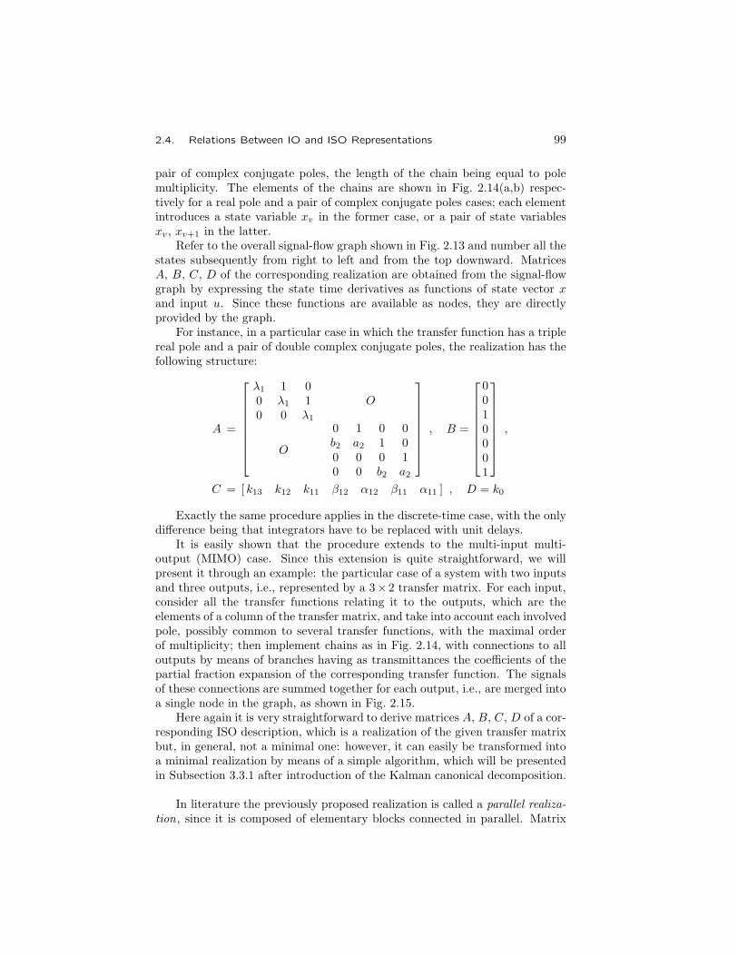
2.4. Relations Between IO and ISO Representations 99
pair of complex conjugate poles, the length of the chain being equal to polemultiplicity. The elements of the chains are shown in Fig. 2.14(a,b) respec-tively for a real pole and a pair of complex conjugate poles cases; each elementintroduces a state variable xv in the former case, or a pair of state variablesxv, xv+1 in the latter.
Refer to the overall signal-flow graph shown in Fig. 2.13 and number all thestates subsequently from right to left and from the top downward. MatricesA, B, C, D of the corresponding realization are obtained from the signal-flowgraph by expressing the state time derivatives as functions of state vector xand input u. Since these functions are available as nodes, they are directlyprovided by the graph.
For instance, in a particular case in which the transfer function has a triplereal pole and a pair of double complex conjugate poles, the realization has thefollowing structure:
A =
⎡⎢⎢⎢⎢⎢⎢⎢⎣
λ1 1 00 λ1 10 0 λ1
O
O
0 1 0 0b2 a2 1 00 0 0 10 0 b2 a2
⎤⎥⎥⎥⎥⎥⎥⎥⎦, B =
⎡⎢⎢⎢⎢⎢⎢⎢⎣
0010001
⎤⎥⎥⎥⎥⎥⎥⎥⎦,
C = [ k13 k12 k11 β12 α12 β11 α11 ] , D = k0
Exactly the same procedure applies in the discrete-time case, with the onlydifference being that integrators have to be replaced with unit delays.
It is easily shown that the procedure extends to the multi-input multi-output (MIMO) case. Since this extension is quite straightforward, we willpresent it through an example: the particular case of a system with two inputsand three outputs, i.e., represented by a 3× 2 transfer matrix. For each input,consider all the transfer functions relating it to the outputs, which are theelements of a column of the transfer matrix, and take into account each involvedpole, possibly common to several transfer functions, with the maximal orderof multiplicity; then implement chains as in Fig. 2.14, with connections to alloutputs by means of branches having as transmittances the coefficients of thepartial fraction expansion of the corresponding transfer function. The signalsof these connections are summed together for each output, i.e., are merged intoa single node in the graph, as shown in Fig. 2.15.
Here again it is very straightforward to derive matrices A, B, C, D of a cor-responding ISO description, which is a realization of the given transfer matrixbut, in general, not a minimal one: however, it can easily be transformed intoa minimal realization by means of a simple algorithm, which will be presentedin Subsection 3.3.1 after introduction of the Kalman canonical decomposition.
In literature the previously proposed realization is called a parallel realiza-tion, since it is composed of elementary blocks connected in parallel. Matrix

100 Chapter 2. General Properties of Linear Systems
chains corresponding
to G11(s), G21(s), G31(s)
chains corresponding
to G12(s), G22(s), G32(s)
u1y1
u2
y2
y3
Figure 2.15. A flow-graph realization of a 3× 2 transfer matrix.
A has a block-companion form. The most significant advantage offered by thisrealization over most of the other known ones is robustness with respect to pa-rameter variations. In fact, the eigenvalues of A, on which the system stabilitydepends, are related to the matrix nonzero coefficients by explicit simple for-mulae, so that their sensitivity to variations of these coefficients is very directand in any case can be easily computed and taken into account.
2.5 Stability
The term stability in the broad sense denotes the capability of a dynamic systemto react with bounded variations of its motion or response to bounded initialstate, input, or parameter perturbations. The notion of stability implies thatthe vector spaces of input, state, output, and parameter vectors and functionsare metric. This will be true for all dynamic systems considered in the sequel.Stability plays a fundamental role in approaching most linear system analysisand synthesis problems, since the property of being stable is required for allactual control system implementations. Hence, in this section we will reviewthe most important mathematical definitions and properties of stability.
2.5.1 Linear Time-Varying Systems
Refer to the linear time-varying free system
x(t) = A(t)x(t) (2.5.1)
The concept of stability is introduced through the following definition which,for linear systems, specializes the well-known concept of stability in the senseof Liapunov.
Definition 2.5.1 (stability in the sense of Liapunov) The linear system(2.5.1) is said to be stable in the sense of Liapunov if for all t0 and for allε> 0 there exists an η > 0 such that
‖x(t0)‖ < η ⇒ ‖x(t)‖ < ε ∀ t ≥ t0 (2.5.2)
2.5. Stability 101
It is said to be asymptotically stable in the sense of Liapunov if, in addition to2.5.2),
limt→∞
‖x(t)‖ = 0 (2.5.3)
The following theorems express stability of system (2.5.1) in terms of tran-sition matrix properties.
Theorem 2.5.1 The linear system (2.5.1) is stable in the sense of Liapunovif and only if for all t0 there exists a real number M such that
‖Φ(t, t0)‖ ≤M <∞ ∀ t ≥ t0 (2.5.4)
Proof. If. Fromx(t) = Φ(t, t0)x(t0)
it follows that‖x(t)‖ ≤ ‖Φ(t, t0)‖ ‖x(t0)‖ ≤M ‖x(t0)‖
hence, by assuming η := ε/M , we derive ‖x(t)‖<ε, t≥ t0, if ‖x(t0)‖<η.Only if. If at a time t1 no value of M exists such that (2.5.4) holds, owing
to the matrix norm inequality
‖A‖ ≤n∑
i=1
n∑j=1
|aij |
there exists at least one element ϕij(t1, t0) of Φ(t1, t0) whose absolute value isunbounded; by assuming an initial state x(t0) with the j-th component equalto η and the others equal to zero, an x(t1) is obtained with the i-th componentunbounded, i.e., an x(t1) unbounded in norm for any value of η; hence, thesystem is not stable. �
Theorem 2.5.2 System (2.5.1) is asymptotically stable in the sense of Lia-punov if and only if (2.5.4) holds for all t0 and
limt→∞
‖Φ(t, t0)‖ = 0 (2.5.5)
Proof. If. Let η := ‖x(t0)‖. Since
‖x(t)‖ ≤ ‖Φ(t, t0)‖ ‖x(t0)‖ = ‖Φ(t, t0)‖ η (2.5.6)
if (2.5.5) holds, the system is asymptotically stable in the origin.Only if. Since for a proper choice of x(t0) relation (2.5.6) holds with
the equality sign, if (2.5.5) were not satisfied it would not be true thatlimt→∞ ‖x(t)‖=0 for all x(t0) such that ‖x(t0)‖> 0. �
Let us refer now to equation (1.3.8) and consider system stability at zerostate with respect to input function perturbations. Since linear systems sta-bility with respect to input function perturbations does not depend on theparticular equilibrium state or on the particular motion referred to, it is possi-ble to define bounded input-bounded state stability as follows.

102 Chapter 2. General Properties of Linear Systems
Definition 2.5.2 (BIBS stability) The linear system (1.3.8) is said to bestable with respect to input function perturbations or bounded input-boundedstate (BIBS) stable if for all t0 and for all ε> 0 there exists an η > 0 such thatfrom ‖u(t)‖<η, t≥ t0 the following holds:
‖x(t)‖ = ‖∫ t
t0
Φ(t, τ)B(τ)u(τ) dτ‖ < ε ∀ t ≥ t0 (2.5.7)
Theorem 2.5.3 The linear system (1.3.8) is BIBS stable if and only if∫ t
t0
‖V (t, τ)‖ dτ :=
∫ t
t0
‖Φ(t, τ)B(τ)‖ dτ ≤M <∞ ∀ t ≥ t0 (2.5.8)
Proof. If. Norms satisfy
‖x(t)‖ = ‖∫ t
t0
Φ(t, τ)B(τ)u(τ) dτ‖ ≤∫ t
t0
‖V (t, τ)‖ ‖u(τ)‖ dτ
and, since ‖u(t)‖≤ η, t≥ t0, it follows that ‖x(t)‖≤Mη, t≥ t0. On the as-sumption η := ε/M equation (2.5.8) clearly holds.
Only if. If equation (2.5.8) is not satisfied, i.e., if there exists a time t1 suchthat the integral ∫ t1
t0
‖V (t1, τ)‖ dτ
is unbounded, the integral ∫ t1
t0
|vij(t1, τ)| dτ
is unbounded for at least one pair of indices i, j. In fact
∫ t1
t0
‖V (t1, τ)‖ dτ ≤∫ t1
t0
n∑r=1
p∑s=1
|vrs(t1, τ)| dτ
=n∑
r=1
p∑s=1
∫ t1
t0
|vrs(t1, τ)| dτ
≤ n p supr,s
∫ t1
t0
|vrs(t1, τ)| dτ
Assume an input function u(t) with the j-th component defined as
uj(t) := η sign (vij(t1, t))
and the other components identically zero. Since
xi(t1) =
∫ t1
t0
vij(t1, τ)uj(τ) dτ = η
∫ t1
t0
|vij(t1, τ)| dτ

2.5. Stability 103
for such an input function, the i-th component of x(t1) is unbounded, i.e., x(t1)is unbounded in norm for any value of η; hence, the system is not BIBS stablein the zero state. �
Bounded input-bounded output stability can be approached in a similarway: the following definition and theorem are derived.
Definition 2.5.3 (BIBO stability) The linear system (1.3.8, 1.3.9) is said tobe bounded input-bounded output (BIBO) stable if for all t0 and all ε> 0 thereexists an η > 0 such that from ‖u(t)‖<η, t≥ t0 it follows that
‖y(t)‖ = ‖C(t)∫ t
t0
Φ(t, τ)B(τ)u(τ) dτ +D(t)u(t)‖ < ε ∀ t ≥ t0 (2.5.9)
Theorem 2.5.4 The linear system (1.3.8, 1.3.9) is BIBO stable if and only if∫ t
t0
‖W (t, τ)‖ dτ =
∫ t
t0
‖C(t)Φ(t, τ)B(τ)‖ dτ ≤M <∞ ∀ t ≥ t0 (2.5.10)
Proof. (Hint) An argument similar to that reported above for Theorem 2.5-3can be used. Furthermore, it is also necessary to take into account the possibledirect action of input on output through matrix D(t). This does not cause anyproblem, since this matrix has been assumed to be bounded in norm for allt. �
The previous definitions and theorems refer to linear time-varying contin-uous systems of type (1.3.8, 1.3.9). Their extension to discrete systems of type(1.3.10, 1.3.11) in the same section is straightforward.
2.5.2 Linear Time-Invariant Systems
The results derived in the previous subsection for general linear time-varyingsystems correspond to a more direct computational framework in the particularcase of linear time-invariant systems.
Consider the linear time-invariant free system
x(t) = Ax(t) (2.5.11)
The main result, which relates stability to the eigenvalues of the system matrix,is stated in the following theorem.
Theorem 2.5.5 The linear system (2.5.11) is stable in the sense of Liapunovif and only if
1. no eigenvalue of A has positive real part;
2. the eigenvalues of A with zero real part are simple zeros of the minimalpolynomial.

104 Chapter 2. General Properties of Linear Systems
Proof. If. Recall that every element of the matrix exponential is a linearcombination of the time functions
eλ1t, t eλ1t, . . . , tm1−1eλ1t, . . . , eλht, t eλht, . . . , tmh−1eλht (2.5.12)
where λi, mi (i=1, . . . , h) denote the distinct eigenvalues of A and theirmultiplicities as zeros of the minimal polynomial. Hence, if conditions 1 and 2hold, i.e., if all modes are stable, it follows that
‖eAt‖ ≤M <∞ ∀ t ≥ 0 (2.5.13)
and, owing to Theorem 2.5.1, the system is stable in the zero state.Only if. It is necessary to prove that all functions (2.5.12) appear in
the elements of the matrix exponential, so that (2.5.13) holds only if 1 and2 are satisfied: if not, the absolute value of at least one element of the matrixexponential would be unbounded at the limit for t approaching infinity. Denoteby B the Jordan form of A. Since B=T−1AT , from (2.5.13) it follows that
‖eBt‖ ≤M ′ <∞ ∀ t ≥ 0
Since the multiplicity of an eigenvalue as a zero of the minimal polynomial isequal to the dimension of the greatest Jordan block of this eigenvalue (see belowfor proof), from relations (2.1.41, 2.1.42) it follows that all functions (2.5.12)are elements of eBt; hence, 1 and 2 are necessary. The minimal polynomial ofA can be written, in factored form, as
m(λ) = (λ− λ1)m1 (λ− λ2)m2 . . . (λ− λh)mh (2.5.14)
Since similar matrices have the same minimal polynomial, m(λ) is the minimalpolynomial of B also. Consider the identity
m(B) = (B − λ1I)m1 (B − λ2I)m2 . . . (B − λhI)mh = O (2.5.15)
The factor (B−λ1I)m1 has the block-diagonal form⎡⎢⎢⎢⎢⎢⎢⎣
(B11−λ1I)m1 . . . O . . . O...
. . ....
. . ....
O . . . (B1,k1 −λ1I)m1 . . . O...
. . ....
. . ....
O . . . O . . . (Bh,kh−λ1I)m1
⎤⎥⎥⎥⎥⎥⎥⎦
(2.5.16)
where the first k1 matrices on the main diagonal, which in the Jordan formcorrespond to the eigenvalue λ1, have the structure⎡
⎢⎢⎢⎢⎢⎢⎣
0 1 0 . . . 0 00 0 1 . . . 0 00 0 0 . . . 0 0...
......
. . ....
...0 0 0 . . . 0 10 0 0 . . . 0 0
⎤⎥⎥⎥⎥⎥⎥⎦

2.5. Stability 105
Denote the dimensions of such matrices with �1j (j=1, . . . , k1): they satisfy
(B1j − λ1I)�1j = O , (B1j − λ1I)�1j−1 �= O
or, in other terms, they are nilpotent of orders �1j. It follows that, if m1≥ �1j(j =1, . . . , k1) all submatrices in (2.5.16) concerning λ1 are zero; hence, thefirst factor in (2.5.15) is zero. The other factors are nonzero, being powers ofupper triangular matrices with nonzero elements on the main diagonal. Thus,relation m(B)=O implies that the value of each mi (i=1, . . . , h) is not lessthan the dimension of the greater Jordan block corresponding to λi. Actuallyit must be exactly equal since, if not, a polynomial nulled by B would existwith lower degree than the minimal polynomial: that obtained by substituting,in (2.5.14), mi with the dimension of the greatest Jordan block correspondingto λi. �
Corollary 2.5.1 The linear system (2.5.11) is stable in the sense of Liapunovif and only if
1. no eigenvalue of A has positive real part;
2. all Jordan blocks corresponding to eigenvalues with zero real part have di-mensions equal to one.
Proof. The proof is contained in that of the previous theorem. �
Theorem 2.5.6 The linear system (2.5.11) is asymptotically stable in thesense of Liapunov if and only if all eigenvalues of A have negative real part.
Proof. Also in this case similarity transformation into the Jordan formprovides the most direct proof argument. Recall Theorem 2.5.2 and definitionsof norms in finite-dimensional vector spaces: it is clear that system (2.5.11)is zero-state stable if and only if every element of eBt tends to zero for tapproaching infinity.Let λ= σ+ jω be a generic eigenvalue of A. Hence
limt→∞
tkeλt = limt→∞
tkeσtejωt = limt→∞
tkeσt(cosωt+ j senωt) = 0
if and only iflimt→∞
tkeσt = 0 (2.5.17)
It is easily seen by using De L’Hospital’s rule that (2.5.17) holds for all non-negative integers k if and only if σ< 0. �
As far as BIBS and BIBO stability are concerned, two interesting resultswill be stated in Subsection 3.3.1, after introduction of the Kalman canonicaldecomposition.

106 Chapter 2. General Properties of Linear Systems
Linear time-invariant discrete systems. The above theorems are easilyextended to linear discrete systems. First, recall that in the discrete-time casemodes, instead of functions of type (2.5.12), there are sequences of the type
λk1 , k λk−11 , . . . , �1!
(k
�1
)λk−�11 , . . . , λkh, k λ
k−1h , . . . , �h!
(k
�h
)λk−�hh (2.5.18)
with �j :=mj − 1 (j=1, . . . , h). In connection with stability of the free system
x(i+1) = Ad x(i ) (2.5.19)
the following results hold. They can be proved by a procedure similar to thatused earlier for continuous systems.
Theorem 2.5.7 The linear system (2.5.19) is stable in the sense of Liapunovif and only if
1. no eigenvalue of A has absolute value greater than one;
2. the eigenvalues of A with absolute value equal to one are simple zeros of theminimal polynomial.
Theorem 2.5.8 The linear system (2.5.19) is asymptotically stable in thesense of Liapunov if and only if all eigenvalues of A have absolute value lessthan one.
2.5.3 The Liapunov and Sylvester Equations
The concept of Liapunov function is basic in the stability theory of nonlinearsystems and will herein briefly be recalled in order to state some interestingresults for the very particular case of linear time-invariant systems. Refer tothe free system
x(t) = f(x(t)) (2.5.20)
where x∈Rn and function f is continuous and satisfies f(0)=0. A continuousfunction V : Rn → R is said to be positive definite in a domain D containingthe origin if V (0)=0 and V (x)> 0 for all x∈D, x �=0. It is called a Lia-punov function if, moreover, V (x) := 〈gradV, f(x)〉≤ 0 for all x∈D, x �=0 . LetDh := {x : V (x) < h}, Dh⊆D. A system that admits a Liapunov function issimply stable at the origin for every initial state belonging to Dh. Furthermore,it is asymptotically stable at the origin for every initial state belonging to Dh
if V (x) is strictly negative for all x∈Dh, x �=0.
The Liapunov Equation. Refer to the free system (2.5.11) and considerthe quadratic form
V (x) = 〈x, Px〉 (2.5.21)
2.5. Stability 107
where P denotes a n×n symmetric, real positive definite matrix. The timederivative along a generic trajectory is
V (x) = 〈Ax, Px〉 + 〈x, PAx〉= 〈x,ATPx〉+ 〈x, PAx〉= −〈x,Mx〉
(2.5.22)
with
M := −(ATP + PA) (2.5.23)
Note that, P being symmetric, M is symmetric. If the quadratic form (2.5.22)is negative definite, function (2.5.21) is a Liapunov function and system (2.5.11)is globally (i.e., for all initial states) asymptotically stable in the zero state. Theequation
ATX +XA = C (2.5.24)
is called a Liapunov matrix equation. The following results point out theimportance of Liapunov equations in connection with stability of linear time-invariant systems.
Lemma 2.5.1 Consider the functional
Γ :=
∫ ∞0
〈x(t),M x(t)〉 dt (2.5.25)
where M denotes any real symmetric matrix, and suppose that matrix A offree system (2.5.11) is strictly stable. The value of Γ along the trajectory of(2.5.11) starting at x0 is
Γ0 = 〈x0, P x0〉 (2.5.26)
where P is the unique solution of the Liapunov equation
AT P + P A = −M (2.5.27)
Proof. Existence and uniqueness of the solution of (2.5.27) are a consequenceof Theorem 2.5.10 reported herein, concerning the Sylvester equation. In fact,A being nonsingular by assumption, matrices A and −AT have no commoneigenvalues (their eigenvalues are nonzero and have opposite sign). Further-more, the solution is a symmetric matrix because the linear function on theleft transforms a symmetric matrix P into a symmetric matrix M and, byuniqueness, the inverse transformation has the same property. Function
s(t) := −〈eAt x0, P eAt x0〉
with P satisfying (2.5.27), is an indefinite integral of
−〈eAt x0,M eAt x0〉

108 Chapter 2. General Properties of Linear Systems
In fact,
s(t) = 〈AeAt x0, P eAt x0〉+ 〈eAt x0, P A e
At x0〉= 〈eAt x0, A
T P eAt x0〉+ 〈eAt x0, P A eAt x0〉
= −〈eAt x0,M eAt x0〉
hence
Γ0 = s(t)∣∣∣t=∞t=0
= 〈x0, P x0〉 �
Theorem 2.5.9 The Liapunov equation (2.5.27) admits a unique, symmetricpositive definite solution P for any symmetric positive definite M if and onlyif matrix A has all eigenvalues with the negative real part.
Proof. If. The statement directly follows from Lemma 2.5.1, since the functionunder the integral sign in (2.5.25) is strictly positive for all x(t) �=0; hence,(2.5.27) is strictly positive for all x0 �=0.
Only if. If (2.5.27) has a positive definite solution P with M positivedefinite, (2.5.21) is a Liapunov function, and system (2.5.11) is asymptoticallystable in the zero state. Thus, A has all eigenvalues with negative real partowing to Theorem 2.5.6. �
The Sylvester Equation. Consider the matrix equation
AX −XB = C (2.5.28)
where A is an m×m matrix, B an n×n matrix, and X and C are both m×n.Equation (2.5.28) is very basic in linear system theory: it is a generalizationof the Liapunov equation and expresses the complementability condition ofan invariant subspace, which recurs in numerous instances in regulation the-ory. Equation (2.5.28) can also be written as the following set of mn scalarequations:
m∑k=1
aikxkj −n∑
k=1
xikbkj = cij (i=1, . . . ,m ; j=1, . . . , n)
or, with a different matrix notation⎡⎢⎢⎣A− b11Im −b21Im . . . −bn1Im−b12Im A− b22Im . . . −bn2Im
......
. . ....
−b1nIm −b2nIm . . . A− bnnIm
⎤⎥⎥⎦
⎡⎢⎢⎣X1
X2...Xn
⎤⎥⎥⎦ =
⎡⎢⎢⎣C1
C2...Cn
⎤⎥⎥⎦
where Xj and Cj (j=1, . . . , n) denote the j-th columns of X and C.By properly redefining matrices, the previous equations can be written in
the formAx = b (2.5.29)

2.5. Stability 109
where A is (mn)× (mn), while x and b are both (mn)× 1. A well-knownnecessary and sufficient condition for equation (2.5.29) to have a solution is
b ∈ imA
A necessary and sufficient condition for the existence and uniqueness of thesolution is stated in the following theorem.
Theorem 2.5.10 Equation (2.5.28) admits a unique solution if and only if Aand B have no common eigenvalues.7
Proof. Only if. Let A and B be respectively m×m and n×n. Equation(2.5.28) is equivalent to a set of nm linear equations with nm unknowns. Itssolution is unique if and only if the corresponding homogeneous equation
AX −XB = O (2.5.30)
admits X =O as the unique solution. Let λ be a common eigenvalue, sothat there exist nonzero vectors (column matrices) u, v such that Av=λ v,BTu=λu, or, for transposes, uTB=λuT . The nonzero matrix X := v uT
satisfies equation (2.5.30). In fact,
Av uT − v uT B = λ v uT − v λuT = O
If. Let σ(B)= {μ1, . . . , μh} be the spectrum of B and
(λ− μi)mij (i=1, . . . , h; j=1, . . . , ki)
the elementary divisors of B: ki is the number of Jordan blocks correspond-ing to the eigenvalue μi and mij (j=1, . . . , ki) their dimensions. It is wellknown that B admits n linearly independent generalized eigenvectors vij�(i=1, . . . , h; j=1, . . . , ki; �=1, . . . ,mij), satisfying
B vij1 = μi vij1
B vij� = μi vij� + vij,�− 1
(i=1, . . . , h; j=1, . . . , ki; �=2, . . . ,mij)
If X is a nonzero solution of (2.5.30), there exists at least one generalizedeigenvector vij� such that X vij� �=0: choose � in the corresponding chain insuch a way that
X vij� �= 0 , X vij,�− 1 = 0
hence
0 = (AX −XB) vij� = AX vij� −X μi vij� = (A− μiI)X vij�
That is, μi is an eigenvalue of A. �7 The proof herein reported is due to Ostrowski and Schneider [24].

110 Chapter 2. General Properties of Linear Systems
Numerical solution of Sylvester equation (hence of Liapunov equation,which is a particular case) can be obtained through the Schur decompositionin the following terms.8
Algorithm 2.5.1 (solution of the Sylvester equation) Consider equation(2.5.24) and perform the Schur decomposition of A and B:
U M U∗X −X V N V ∗ = C
where U and V are unitary, M and N upper-triangular complex matrices.Premultiply by U∗ and postmultiply by V , thus obtaining
M D −DN = G with D := U∗X V , G := U∗ C V
which can be directly solved by
D1 = (M − n11 Im)−1G1
Di = (M − nii Im)−1(Gi +
i−1∑j=1
njiDj
)(i=2, . . . , n)
where Di and Gi (i=1, . . . , n) denote the i-th columns of D and G. Thencompute X =U DV ∗. �
2.6 Controllability and Observability
It will be shown that the sets defined in Section 1.4 assume particular structuresfor linear systems, so that procedures to solve general control and observationproblems can easily be derived.
2.6.1 Linear Time-Varying Systems
A basic property of the sets of states reachable from the origin and of statescontrollable to the origin is as follows.
Property 2.6.1 In the case of linear time-varying systems the reachable setfrom the origin R+(t0, t1, 0) and the controllable set to the origin R−(t0, t1, 0)are subspaces of the state space X .
Proof. The set R+(t0, t1, 0) is a subspace, being the image of the lineartransformation ϕ(t1, t0, 0, u(·)) from Uf to X . R−(t0, t1, 0) can be defined as{
x : (x, u(·)) ∈ N}
(2.6.1)
8 This method and Fortran programs for its implementation were proposed by Bartelsand Stewart [2].

2.6. Controllability and Observability 111
where N denotes the subset of X ×Uf defined by
N :={(x, u(·)) : 0 = ϕ
(t1, t0, x, u(·)
)}which is a subspace, being the kernel of a linear transformation. The set (2.6.1)is a subspace, being the projection of a subspace. �
On the other hand, the setsW+(t0, t1, 0) andW−(t0, t1, 0) are not generallysubspaces in the case of time-varying systems.9 It will be shown in the nextsubsection that, on the contrary, they are subspaces in the case of linear time-invariant systems.
As a consequence of Properties 2.6.1 and 1.3.4 (decomposability of motion),the following statement holds.
Property 2.6.2 In the case of linear time-varying systems the setR+(t0, t1, x0) is the linear variety defined as the sum of subspace R+(t0, t1, 0)and any state reachable from x0 in [t0, t1], while the set R−(t0, t1, x1) is thelinear variety defined as the sum of the subspace R−(t0, t1, 0) and any statefrom which x1 can be reached in [t0, t1].
Now we shall examine some computational aspects of control. Refer to thelinear time-varying system (1.3.8, 1.3.9) and consider the problem of computingbasis matrices for the subspaces R+(t0, t1, 0) and R−(t0, t1, 0).10
The following lemma will be the basic tool to derive the main results.
Lemma 2.6.1 Let F (·) be an n×m matrix whose elements are piecewise con-tinuous functions in [t0, t1] with values in R
m. The equality
FT (t)x = 0 ∀ t ∈ [t0, t1] (2.6.2)
holds if and only if x ∈ kerG(t0, t1), where G(t0, t1) denotes the Gramian matrixdefined as
G(t0, t1) :=
∫ t1
t0
F (t)FT (t) dt (2.6.3)
9 This can be shown with a simple example. Consider a linear discrete system describedby equations (1.3.10, 1.3.11), with
Ad(0) := Ad(1) :=
[0 01 0
], Bd(0) :=
[10
], Bd(1) :=
[01
]
Let Ad :=Ad(0)=Ad(1); clearly
R+(0, 1, 0) = imBd(0)
R+(0, 2, 0) = Ad imBd(0) + imBd(1)
and, since Ad imBd(0)= imBd(1), it follows that
W+(0, 2, 0) := R+(0, 1, 0) ∪R+(0, 2, 0) = imBd(0) ∪ imBd(1)
which shows that W+(0, 2, 0) is not a subspace.10 A generic subspace S ∈Rn is numerically determined by means of a matrix S such that
S =imS, which is called a basis matrix of S.
112 Chapter 2. General Properties of Linear Systems
Proof. MatrixG(t0, t1) is symmetric, being the integral of a symmetric matrix.Furthermore
〈x,G(t0, t1)x〉 =∫ t1
t0
‖FT (t)x‖ 22 dt ∀ x ∈ Rn
hence G(t0, t1) is positive semidefinite and any x∈Rn such that〈x,G(t0, t1)x〉=0 also satisfies the equality FT (t)x=0 for all t∈ [t0, t1] andvice versa. On the other hand, owing to Theorem A.5.4 from G(t0, t1)being positive semidefinite it follows that 〈x,G(t0, t1)x〉=0 if and only ifx∈ kerG(t0, t1). �
If relation (2.6.2) holds for x �=0, the rows of F (·) are linearly dependent in[t0, t1] by definition, so that the rows of F (·) are linearly independent in [t0, t1]if and only if G(t0, t1) is nonsingular.
Theorem 2.6.1 Refer to system (1.3.8, 1.3.9). The following equalities hold.
R+(t0, t1, 0) = imP (t0, t1) (2.6.4)
R−(t0, t1, 0) = Φ−1(t1, t0) imP (t0, t1) = Φ(t0, t1) imP (t0, t1) (2.6.5)
where P (t0, t1) denotes the symmetric positive semidefinite matrix
P (t0, t1) :=
∫ t1
t0
Φ(t1, τ)B(τ)BT (τ)ΦT (t1, τ) dτ (2.6.6)
Proof. Since kerP (t0, t1)= (imP (t0, t1))⊥, to prove (2.6.4) it is sufficient to
show that the nonzero states belonging to kerP (t0, t1) are not reachable fromthe origin in [t0, t1], while those belonging to imP (t0, t1) are reachable. Supposethat a state x1 is reachable from the origin in [t0, t1]; hence there exists an inputfunction u(·) such that
x1 =
∫ t1
t0
Φ(t1, τ)B(τ)u(τ) dτ (2.6.7)
Let x1 ∈ kerP (t0, t1). The left scalar product of both members of the previousrelation by x1 gives
〈x1, x1〉 =∫ t1
t0
〈BT (τ)ΦT (t1, τ)x1 , u(τ)〉 dτ
Owing to Lemma 2.6.1, BT (t)ΦT (t1, t)x1 =0 for all t∈ [t0, t1], so that for anyinput function u(·) condition x1 ∈ kerP (t0, t1) implies x1 =0. On the otherhand, let x1 ∈ imP (t0, t1), so that
x1 = P (t0, t1)P+(t0, t1)x1

2.6. Controllability and Observability 113
where P+(t0, t1) denotes the pseudoinverse of P (t0, t1); by using (2.6.6) theprevious expression can be written as
x1 =
∫ t1
t0
Φ(t1, τ)B(τ)BT (τ)ΦT (t1, τ)P+(t0, t1)x1 dτ
which, by comparison with (2.6.7), states that x1 is reachable from the originwith the particular input
u(t) := BT (t)ΦT (t1, t)P+(t0, t1)x1 (2.6.8)
To prove (2.6.5), note that relation x0 ∈R−(t0, t1, 0) implies the existence ofan input function u(·) such that
0 = Φ(t1, t0)x0 +
∫ t1
t0
Φ(t1, τ)B(τ)u(τ) dτ
i.e.,−Φ(t1, t0)x0 ∈ R+(t0, t1, 0)
hencex0 ∈Φ−1(t1, t0)R+(t0, t1, 0) = Φ(t0, t1)R+(t0, t1, 0)
This completes the proof. �
In conclusion, system (1.3.8, 1.3.9) is completely controllable and com-pletely reachable in [t0, t1] (i.e., R+(t0, t1, 0)=R−(t0, t1, 0)=Rn, henceR+(t0, t1, x)=R−(t0, t1, x)=Rn for all x∈Rn) if and only if matrix P (t0, t1),defined in (2.6.6), is nonsingular (strictly positive definite).
Problem 2.6.1 (control between two given states) Refer to system(1.3.8, 1.3.9). Determine an input function u(·) which produces transition be-tween two arbitrarily given states x0, x1 in the time interval [t0, t1].
Solution. By linearity, the input function that solves the problem also drivesthe system from the origin to x2 :=x1−Φ(t1, t0)x0, so that, for the problemto have a solution, relation x2 ∈R+(t0, t1, 0) must be satisfied. Recall (2.6.8):it is possible to assume
u(t) := BT (t)ΦT (t1, t)P+(t0, t1)x2 , t∈ [t0, t1] (2.6.9)
Owing to a well-known feature of the pseudoinverse matrix, such a controlfunction provides the best approximation (in euclidean norm) to the final statex1 when this is not reachable from x0. �
Matrix P (t0, t1) can be computed by the following procedure: denote byΦ(·, ·) the state transition matrix corresponding to the system matrix
A(t) :=
[A(t) B(t)BT (t)O −AT (t)
](2.6.10)

114 Chapter 2. General Properties of Linear Systems
and by M the submatrix corresponding to the first n rows and the last ncolumns of Φ(t1, t0). Then
P (t0, t1) =M ΦT (t1, t0) (2.6.11)
where Φ(·, ·) denotes the transition matrix corresponding to A(t). Computationis particularly simple in the case of time-invariant systems, where
Φ(T, 0) = eAT , ΦT (T, 0) = eATT
Extension of the preceding material on the state controllability to the out-put controllability is relatively simple, since “pointwise” output controllabilityis easily reconducted to state controllability. Continuous or “functional” out-put controllability will be investigated in Section 4.3 by using the geometricapproach.
We shall now consider observability of linear time-varying systems. The setsQ−(t0, t1, u(·), y(·)) andQ+(t0, t1, u(·), y(·)), defined in Section 1.4, have specialfeatures in the linear system case, owing to Property 1.3.4 (decomposability ofthe response function). The following two properties will be proved together.
Property 2.6.3 Like any other system, a linear system completely observablein [t0, t1] is also reconstructable in [t0, t1]. The converse is also true in the caseof linear continuous systems.
Property 2.6.4 A linear system completely observable by a diagnosis experi-ment or reconstructable by a homing experiment is simply completely observableor reconstructable. In other words, for linear systems there is no advantage inusing a special input function to derive the initial or final state from the re-sponse function.
Proof. The response decomposition property implies that
Q−(t0, t1, u(·), y(·)
)={
x : y(τ) = γ(τ, t0, x, 0) + γ(τ, t0, 0, u(·)
), τ ∈ [t0, t1]
}Assume y1(t) := γ(t, t0, 0, u(·)). It follows that
Q−(t0, t1, u(·), y(·)
)=
Q−(t0, t1, 0, y(·)− y1(·)
)= Q−
(t0, t1, 0, y0(·)
)(2.6.12)
where y0(·) := y(·)− y1(·) denotes the free response, which depends only on thestate at time t0. Then, from (1.4.10)
Q+(t0, t1, u(·), y(·)
)=
Φ(t1, t0)Q−(t0, t1, 0, y0(·)
)+
{ϕ(t1, t0, 0, u(·)
)}(2.6.13)
If the set (2.6.12) reduces to a single element, (2.6.13) also does, while thecontrary is true only if matrix Φ(t1, t0) is nonsingular, i.e., in particular, for

2.6. Controllability and Observability 115
continuous systems. If the set (2.6.12) or the set (2.6.13) reduces to a singleelement, this occurs independently on input u(·). �
Property 2.6.5 In the case of linear systems the sets Q−(t0, t1, 0, 0),Q+(t0, t1, 0, 0) are subspaces of X .
Proof. The set Q−(t0, t1, 0, 0) is a subspace, being the kernel of the lin-ear transformation from X to Yf which associates to any x∈X functiony(τ)= γ(τ, t0, x, 0), τ ∈ [t0, t1]. The set Q+(t0, t1, 0, 0) is a subspace, being itsimage in the linear transformation from X to X corresponding to the transitionmatrix Φ(t1, t0). �
The following result is a consequence of zero-input response linearity.
Property 2.6.6 In the case of linear systems the set Q−(t0, t1, 0, y0(·)) isthe linear variety defined as the sum of any initial state corresponding tofree response y0(·) in [t0, t1] and the subspace Q−(t0, t1, 0, 0), while the setQ+(t0, t1, 0, y0(·)) is the linear variety defined as the sum of any initial statecorresponding to free response y0(·) in [t0, t1] and the subspace Q+(t0, t1, 0, 0).
Computational aspects of observation problems for linear systems are sim-ilar to those of control problems. First of all, we shall consider determinationof the subspaces Q−(t0, t1, 0, 0) and Q+(t0, t1, 0, 0).
Theorem 2.6.2 Refer to system (1.3.8, 1.3.9). The following equalities hold.
Q−(t0, t1, 0, 0) = kerQ(t0, t1) (2.6.14)
Q+(t0, t1, 0, 0) = Φ(t1, t0) kerQ(t0, t1) (2.6.15)
where Q(t0, t1) denotes the symmetric positive semidefinite matrix
Q(t0, t1) :=
∫ t1
t0
ΦT (τ, t0)CT (τ)C(τ)Φ(τ, t0) dτ (2.6.16)
Proof. Owing to Lemma 2.6.1, the relation
y0(t) = C(t)Φ(t, t0)x0 = 0 ∀ t∈ [t0, t1]
is satisfied if and only if x0 ∈ kerQ(t0, t1). On the other hand, if the initial statex0 belongs to imQ(t0, t1), it can be uniquely determined from the free responsey0(t). In fact, by using (2.6.16) in the equality x0 =Q+(t0, t1)Q(t0, t1)x0, itfollows that
x0 = Q+(t0, t1)
∫ t1
t0
ΦT (τ, t0)CT (τ)C(τ)Φ(τ, t0)x0 dτ
i.e.,
x0 = Q+(t0, t1)
∫ t1
t0
ΦT (τ, t0)CT (τ) y0(τ) dτ (2.6.17)

116 Chapter 2. General Properties of Linear Systems
Relation (2.6.15) directly follows from (2.6.13). �
As a consequence of the previous theorem, it can be stated that sys-tem (1.3.8, 1.3.9) is completely observable and reconstructable in [t0, t1] (i.e.,Q−(t0, t1, 0, 0)=Q+(t0, t1, 0, 0)= {0}) if and only if matrix Q(t0, t1) defined in(2.6.16) is nonsingular (strictly positive definite).
Problem 2.6.2 (observing the initial state) Refer to system (1.3.8, 1.3.9).Given functions u(·), y(·) in the time interval [t0, t1], determine the initialstate x0.
Solution. Derive the free response
y0(t) = y(t)− C(t)∫ t
t0
Φ(t, τ)B(τ)u(τ) dτ −D(t)u(t)
and use (2.6.17). Owing to a property of the pseudoinverse matrix, the rightside of (2.6.17) directly provides the orthogonal projection of the initial stateon the orthogonal complement of Q−(t0, t1, 0, 0); this coincides with x0 if thesystem is completely observable. �
The problem of reconstructing final state x1, or its orthogonal projectionx2 on the orthogonal complement of Q+(t0, t1, 0, 0) when the system is notcompletely reconstructable, can be solved in a similar way. If the system iscompletely observable, i.e., if the problem of determining the initial state hasa unique solution, from (2.2.2) with t= t1 it is possible to derive x1 if x0 isknown.
To solve Problem 2.6.2 from a computational standpoint it is still conve-nient to use the adjoint system. In fact, consider the system
p(t) = −AT (t) p(t) + CT (t) y0(t) (2.6.18)
with initial condition p(t0)= 0. Solving in [t0, t1] provides
p(t1) =
∫ t1
t0
Ψ(t1, τ)CT (τ) y0(τ) dτ
= ΦT (t0, t1)
∫ t1
t0
ΦT (τ, t0)CT (τ) y0(τ) dτ
By comparison with (2.6.17), if the system is completely observable (hencematrix Q(t0, t1) is invertible), the initial state can be derived as
x0 = Q−1(t0, t1)Ψ(t0, t1) p(t1) (2.6.19)
The observation or reconstruction of the state can be realized “on line”as follows: by means of a model of system (1.3.8, 1.3.9) with zero initial statedetermine the forced response y1(·) and subtract it from the output function
2.6. Controllability and Observability 117
to obtain the free response y0(·), which, in turn, is the input function to theadjoint system (2.6.18), whose solution with zero initial condition provides thevalue p(t1) to use in (2.6.19). The final state owing to (2.2.2) is expressed as
x1 = Φ(t1, t0)Q−1(t0, t1)Ψ(t0, t1) p(t1) + ϕ1(t1)
where ϕ1(t1) is the final value of the forced motion.
Extension to Discrete Systems. The extension of the above to discretesystems is straightforward, so that we shall report the main results withoutproof.
Refer to system (1.3.10, 1.3.11). The following equalities hold.
R+(j, i, 0) = imP (j, i ) (2.6.20)
R−(j, i, 0) = Φ−1(i, j ) imP (j, i ) (2.6.21)
where P (j, i ) denotes the symmetric positive semidefinite matrix
P (j, i ) :=
i−1∑k=j
Φ(i, k+1)Bd(k)BTd (k)Φ
T (i, k+1)
The problem of controlling the state trajectory between two given statesx0, x1 in the time interval [j, i] is solved by
u(k) = BTd (k)Φ
T (i, k+1)P+(j, i )x2 , k ∈ [j, i− 1] (2.6.22)
with x2 := x1−Φ(i, j )x0.The subspaces of the initial and final states corresponding to zero response
in the time interval [j, i ] for system (1.3.10, 1.3.11) are, respectively
Q−(j, i, 0, 0) = kerQ(j, i ) (2.6.23)
Q+(j, i, 0, 0) = Φ(i, j ) kerQ(j, i ) (2.6.24)
where Q(j, i ) denotes the symmetric positive semidefinite matrix
Q(j, i ) :=
i∑k=j
ΦT (k, j )CTd (k)Cd(k)Φ(k, j )
The problem of determining the initial state x0 (or its orthogonal projec-tion on the orthogonal complement of Q−(j, i, 0, 0) when the system is notcompletely observable) from functions u(·), y(·) given in the time interval [j, i ],can be solved by means of
y0(k) = y(k)− Cd(k)
k−1∑h=j
Φ(k, h+1)Bd(h)u(h) −
Dd(k)u(k), k ∈ [j, i] (2.6.25)
x0 = Q+(j, i )
i∑k=j
ΦT (k, j )CTd (k) y0(k) (2.6.26)

118 Chapter 2. General Properties of Linear Systems
2.6.2 Linear Time-Invariant Systems
Consistent with notation introduced in Section 1.4, denote by R+t1(x) the
reachable set from x in [0, t1] and by R−t1(x) the controllable set to x in [0, t1].
By Property 2.6.1 R+t1(0) and R−t1(0) are subspaces of X , while by Property
2.6.2 R+t1(x) and R
−t1(x) are linear varieties contained in X .
Property 2.6.7 In the case of linear time-invariant systems the followinginclusions hold:
R+t1(0) ⊆ R
+t2(0) for t1 ≤ t2 (2.6.27)
R−t1(0) ⊆ R−t2(0) for t1 ≤ t2 (2.6.28)
Proof. Let x1 ∈R+t1(0), so that a control function u1(t), t∈ [0, t1] exists, which
drives the state from zero to x1 at time t1; the control function defined asu2(t)= 0 for t∈ [0, t2− t1] and u2(t)=u1(t− t2 + t1) for t∈ [t2− t1, t2] clearlydrives the state from zero to x1 at time t2, hence (2.6.27) holds. A similarargument proves (2.6.28). �
The following corollary is an immediate consequence of Property 2.6.7.
Corollary 2.6.1 In the case of linear time-invariant systems the followingequalities hold:
W+t1(0) = R+
t1(0) (2.6.29)
W−t1 (0) = R−t1(0) (2.6.30)
Let us consider, in particular, linear time-invariant continuous systems.The basic result for controllability is stated in the following theorem.
Theorem 2.6.3 Refer to system (2.2.15, 2.2.16). The reachable set from theorigin in [0, t1] is
R+t1(0) = imP with P := [B AB . . . An−1B] (2.6.31)
Proof. From Lemma 2.6.1 and Theorem 2.6.1 it follows that any x1 such that
x1 ∈ R+t1(0)
⊥ (2.6.32)
satisfies
BT ΦT (t1, τ)x1 = 0 ∀ τ ∈ [0, t1] (2.6.33)
and, conversely, (2.6.32) holds for all x1 satisfying (2.6.33). Let t := t1− τ , sothat (2.6.33) is written as
BT eAT t x1 = 0 ∀ t ∈ [0, t1] (2.6.34)

2.6. Controllability and Observability 119
Since the function on the left of (2.6.34) is analytic and identically zero in theinterval [0, t1], all its derivatives are also identically zero. Differentiating att=0 yields
BT (AT )i x1 = 0 (i = 0, . . . , n− 1) (2.6.35)
In (2.6.35) it is not necessary to consider powers higher than n− 1. In fact, theCayley-Hamilton theorem implies
An = −(a1An−1 + a2An−2 + . . .+ an I)
hence
An B = −(a1An−1B + a2An−2B + . . .+ anB) (2.6.36)
Transpose and multiply on the right by x1. Then
BT (AT )n x1 = −(a1BT (AT )n−1 x1 + . . .+ anBT x1)
so that (2.6.35) are satisfied also for i≥n. Recall the matrix exponential powerseries expansion: clearly relations (2.6.35) are not only necessary, but alsosufficient for (2.6.34) to hold. On the other hand, (2.6.35) are equivalent tox1 ∈ kerPT . Since (2.6.34) is satisfied if and only if (2.6.32) holds, (2.6.31) isproved. �
The following property expresses Theorem 2.6.3 in coordinate-free formand can be considered as a first step towards a geometric settling of thecontrollability and observability concepts.
Property 2.6.8 Refer to system (2.2.15, 2.2.16). The reachable set from theorigin in [0, t1] can be expressed as
R+t1(0) = minJ (A,B) (2.6.37)
where minJ (A,B) denotes the minimal A-invariant containing B := imB.11
Proof. It has already been proved that imP is an A-invariant. Since all thecolumns of matrix P clearly belong to all other A-invariants containing B, imPcoincides with minJ (A,B). �
Property 2.6.9 Refer to system (2.2.15, 2.2.16). The controllable set to theorigin is equal to the reachable set from the origin, i.e.,
R−t1(0) = R+t1(0) (2.6.38)
11 The set of all A-invariants containing a given subspace B is a non-distributive latticewith respect to ⊆,+,∩, which admits a supremum, the whole space X , and an infimum,minJ (A,B).

120 Chapter 2. General Properties of Linear Systems
Consider (2.6.5), which in this case can be written as
R−t1(0) = e−At1 R+t1(0)
and note that any A-invariant is also an invariant with respect to eAt ande−At, as immediately follows from the power series expansion of the matrixexponential; equality (2.6.38) is implied by e−At1 being nonsingular. �
It is remarkable that the expressions for R+t1(0) and R
−t1(0) derived earlier
are independent of t1, i.e., in the case of linear time-invariant continuoussystems the reachable subspace and the controllable subspace do not dependon the length of time for control, provided it is nonzero.
From now on, the simple symbol R will be used for many sets referring tocontrollability of linear time-invariant continuous systems:
R := minJ (A,B) = R+t1(0) = R
−t1(0) =W
+t1(0) =W
−t1 (0) (2.6.39)
The subspace B := imB will be called the forcing actions subspace and Rthe controllability set or controllability subspace. System (2.2.15, 2.2.16) willbe said to be completely controllable if R=X . In this case it is also customaryto say that the pair (A,B) is controllable.
Observability of linear time-invariant systems is now approached in a simi-lar way. Denote byQ−t1(u(·), y(·)) andQ
+t1(u(·), y(·)) the sets of all initial and fi-
nal states compatible with input function u(·) and output function y(·) in [0, t1],also called the unobservable set and the unreconstructable set in [0, t1] with re-spect to the given input and output functions. By Property 2.6.5 Q−t1(0, 0)and Q+
t1(0, 0) are subspaces of X , while by Property 2.6.6 Q−t1(u(·), y(·)) and
Q+t1(u(·), y(·)) are linear varieties contained in X .
Property 2.6.10 In the case of linear time-invariant systems the followingequalities hold:
Q−t1(0, 0) ⊇ Q−t2(0, 0) for t1 ≤ t2 (2.6.40)
Q+t1(0, 0) ⊇ Q
+t2(0, 0) for t1 ≤ t2 (2.6.41)
Proof. Initial states belonging to Q−t2(0, 0) cause zero free response in the
time interval [0, t2], which contains [0, t1], so that they also belong to Q−t1(0, 0)and (2.6.40) is proved. A similar argument proves (2.6.41). �
Let us consider, in particular, linear time-invariant continuous systems.The most important result of observability is stated in the following theorem,dual of Theorem 2.6.3.
Theorem 2.6.4 Refer to system (2.2.15, 2.2.16). The zero-input unobservableset in [0, t1] is
Q−t1(0, 0) = kerQ with QT := [CT ATCT . . . (AT )n−1CT ] (2.6.42)

2.6. Controllability and Observability 121
Proof. From Lemma 2.6.1 and Theorem 2.6.2 it follows that any x0 such that
x0 ∈ Q−t1(0, 0) (2.6.43)
satisfiesC Φ(τ, 0)x0 = 0 ∀ τ ∈ [0, t1] (2.6.44)
and, conversely, (2.6.43) holds for all x0 satisfying (2.6.44). Relation (2.6.44)can also be written as
C eAτ x0 = 0 ∀ τ ∈ [0, t1] (2.6.45)
and by the argument considered in the proof of Theorem 2.6.3 conditionx0 ∈ kerQ is proved to be necessary and sufficient for (2.6.43) to hold. �
Theorem 2.6.4 can be stated in coordinate-free form as follows.
Property 2.6.11 Refer to system (2.2.15, 2.2.16). The zero-input unobserv-able set in [0, t1] can be expressed as
Q−t1(0) = maxJ (A, C) (2.6.46)
where maxJ (A, C) denotes the maximal A-invariant contained in C := kerC.12
Proof. From the proof of Property 2.6.8 it follows that imQT is the minimalAT -invariant containing imCT , so that its orthogonal complement kerQ is themaximal A-invariant contained in kerC. �
Property 2.6.12 Refer to system (2.2.15, 2.2.16). The zero-input unrecon-structable set in [0, t1] is equal to the zero-input unobservable set, i.e.,
Q+t1(0, 0) = Q
−t1(0, 0) (2.6.47)
Proof. Consider (2.6.15), which in this case can be written as
Q+t1(0, 0) = eAt1 Q−t1(0, 0)
Equality (2.6.47) follows from Q−t1(0, 0) being an A-invariant, hence an invari-ant also with respect to eAt1 and from the matrix exponential being nonsingu-lar. �
The above expressions for Q−t1(0, 0) and Q+t1(0, 0) are independent of t1,
so that in the case of linear time-invariant continuous systems the zero-inputunobservable subspace and the zero-input unreconstructable subspace do notdepend on the length of time for observation, provided it is nonzero.
12 The set of all A-invariants contained in a given subspace C is a nondistributive latticewith respect to ⊆,+,∩, which admits a supremum, maxJ (A, C), and an infimum, theorigin {0}.

122 Chapter 2. General Properties of Linear Systems
In the following, the simple symbol Q will be used for both:
Q := maxJ (A, C) = Q−t1(0, 0) = Q+t1(0, 0) (2.6.48)
The subspace C := kerC will be called the inaccessible states subspace andQthe unobservability set or unobservability subspace. System (2.2.15, 2.2.16) willbe said to be completely observable if Q= {0}. In this case it is also customaryto say that the pair (A,C) is observable.
Extension to Discrete Systems. We shall now extend the results oncontrollability and observability to linear time-invariant discrete systems. Referto system (2.2.17, 2.2.18): let R+
i (0) be the reachable set from the origin in isteps. It is easy to see that
R+i (0) = imPi with Pi := [Bd Ad Bd . . . Ai−1
d Bd] (i=1, 2, . . . ) (2.6.49)
In fact, let x1 ∈R+i (0)
⊥. From (2.6.20) and Theorem A.5.4 it follows thatBT
d (ATd )
ix1 =0, hence x1 ∈ kerPTi . The Cayley-Hamilton theorem implies that
the maximal reachable subspace is attained in a number of steps not greaterthan n. It coincides with the minimal Ad-invariant containing the forcing actionsubspace Bd := imBd, i.e., R+(0) := limi→∞R+
i (0)=R+n (0)=minJ (Ad,Bd).
The controllable set to the origin in i steps is determined from(2.6.21) asR−i (0)=A−id R
+i (0). Moreover,R−(0) := limi→∞R−i (0)=R−n (0) =
A−nd minJ (Ad,Bd).The zero-input unobservable subspace in i steps Q−i (0, 0) (i=0, 1, . . . ) is
expressed by
Q−i (0, 0) = kerQi with QTi := [CT
d ATd CT
d . . . (ATd )
i CTd ] (i=0, 1, . . . )
(2.6.50)In fact, let x0 ∈Q−i (0, 0)⊥. From (2.6.23) and Theorem A.5.4 it fol-lows that CdA
idx0 =0, hence x0 ∈ kerQT
i . The Cayley-Hamilton theoremimplies that the minimal unobservable subspace corresponds to a num-ber of steps not greater than n− 1. It coincides with the maximal Ad-invariant contained in the inaccessible states subspace Cd := kerCd, i.e.,Q−(0, 0) := limi→∞Q−i (0, 0)=Q−n−1(0, 0)=maxJ (Ad, Cd).
The zero-input unreconstructable subspace in i steps is determined from(2.6.24) as Q+
i (0, 0)=AidQ−i (0, 0). Moreover, Q+(0, 0) := limi→∞Q+
i (0, 0) =Q+
n (0, 0)=And maxJ (Ad, Cd).
As for the continuous system, we define R :=R+(0)=minJ (Ad,Bd) andQ :=Q−(0, 0)=maxJ (Ad, Cd). However, for discrete systems the equalitiesR−(0)=R+(0) and Q−(0, 0)=Q+(0, 0) are not true in general. They are re-placed by the inclusions R−(0)⊇R+(0) and Q−(0, 0)⊇Q+(0, 0), which derivefrom the general property that if J is an A-invariant, both AJ and A−1J areA-invariants, hence, by a recursion argument, AiJ and A−iJ (i=2, 3, . . . ) areA-invariants.
References

References 123
1. Aizerman, M.A., and Gantmacher, F.R., Absolute Stability of RegulatorSystems, Holden-Day, San Francisco, 1964.
2. Bartels, R.H., and Stewart, G.W., “Solution of the matrix equationAX+XB=C,” Communications of the ACM , vol. 15, no. 9, pp. 820–826, 1972.
3. Bellman, R., Stability Theory of Differential Equations, McGraw-Hill, NewYork, 1953.
4. Brockett, R.W., Finite Dimensional Linear Systems, Wiley, New York, 1970.
5. Byers, R., “A LINPACK-style condition estimator for the equation AX−XBT =C,” IEEE Trans. on Aut. Control , vol. AC-29, pp. 926–928, 1984.
6. Callier, F.M., and Desoer, C.A., Multivariable Feedback Systems,Springer-Verlag, New York, 1982.
7. Chen, C.T., Introduction to Linear System Theory , Holt, Rinehart & Winston,New York, 1970.
8. — , Linear System Theory and Design, Holt, Rinehart & Winston, New York,1984.
9. De Russo, P.M., Roy, R.I., and Close, C.M., State Variables for Engi-neers, Wiley, New York, 1967.
10. Hahn, W., Theory and Application of Liapunov’s Direct Method , Prentice Hall,Englewood Cliffs, N.J., 1963.
11. Hale, J.K., Oscillation in Nonlinear Systems, McGraw-Hill, New York, 1963.
12. Kalman, R.E., “On structural properties of linear, constant, multivariablesystems,” Proceedings of the 3rd IFAC Congress, paper 6a, 1966.
13. Kalman, R.E., and Bertram, J.E., “Control system analysis and designvia the second method of Liapunov - I Continuous-time systems,” Trans. of theASME, J. of Basic Engineering , vol. 82, pp. 371–393, 1960.
14. — , “Control system analysis and design via the second method of Liapunov -II Discrete-time systems,” Trans. of the ASME, J. of Basic Engineering , vol. 82,pp. 394–400, 1960.
15. La Salle, J., and Lefschetz, S., Stability by Liapunov’s Direct Method withApplications, Academic, New York, 1961.
16. Lefschetz, S., Stability of Nonlinear Control Systems, Academic, New York,1965.
17. Liapunov, A.M., “Probleme general de la stabilite du mouvement,” Ann. Fac.Sci. Toulouse, vol. 9, pp. 203–474, 1907.
18. Luenberger, D.G., “Invertible solutions to the operator equation TA-BT=C,”Proc. Am. Math. Soc., vol. 16, pp. 1226–1229, 1965.
19. MacFarlane, A.G.J., “System matrices,” Proc. IEE , vol. 115, no. 5, pp.749–754, 1968.
20. — , “The development of frequency-response methods in automatic control,”IEEE Trans. Autom. Control , vol. AC-24, no. 2, pp. 250–265, 1979.
21. Minorsky, N., Introduction to Nonlinear Mechanics, J. W. Edwards, AnnArbor, 1947.
22. Molinari, B.E., “Algebraic solution of matrix linear equations in controltheory,” Proc. IEE , vol. 116, pp. 1748–1754.

124 Chapter 2. General Properties of Linear Systems
23. Ogata, K., State Space Analysis of Control Systems, Prentice Hall, EnglewoodCliffs, N.J., 1967.
24. Ostrowski, A., and Schneider, H., “Some theorems on the inertia ofgeneral matrices,” J. of Math. Analysis and Applications, vol. 4, pp. 72–84, 1962.
25. Rosenbrock, H.H., “Transformation of linear constant system equations,”Proc. IEE , vol. 114, no. 4, pp. 541–544, 1967.
26. — , “On linear system theory,” Proc. IEE , vol. 114, no. 9, pp. 1353–1359, 1967.
27. — , “Computation of minimal representations of a rational transfer-functionmatrix,” Proc. IEE , vol. 115, no. 2, pp. 325–327, 1968.
28. — , State-space and Multivariable Theory , Nelson, London, 1970.
29. Rosenbrock, H.H., and Storey, C., Mathematics of Dynamical Systems,Nelson, London, 1970.
30. Sansone, G., and Conti, R., Equazioni Differenziali Non Lineari , EdizioniCremonese, Rome, 1956.
31. Schultz, D.G., and Melsa, J.L., State Function and Linear Control Sys-tems, McGraw-Hill, New York, 1967.
32. Tou, J.T., Modern Control Theory , McGraw-Hill, New York, 1964.
33. Varah, J.M., “On the separation of two matrices,” SIAM J. Numer. Anal.,vol. 16, pp. 216–222, 1979.
34. Vidyasagar, M., Nonlinear System Analysis, Prentice Hall, Englewood Cliffs,N.J., 1978.
35. Vidyasagar, M., Control System Synthesis: A Factorization Approach, TheMIT Press, Cambridge, Mass., 1985.
36. Willems, J.L., Stability Theory of Dynamical Systems, Wiley, New York, 1970.
Chapter 3
The Geometric Approach:Classic Foundations
3.1 Introduction
The essence of the geometric approach consists of developing most of the math-ematical support in coordinate-free form, to take advantage of simpler and moreelegant results, which facilitate insight into the actual meaning of statementsand procedures; the computational aspects are considered independently of thetheory and handled by means of the standard methods of matrix algebra, oncea suitable coordinate system is defined. The cornerstone of the approach is theconcept of invariance of a subspace with respect to a linear transformation. Inthis chapter the properties and geometric meaning of invariants are presentedand investigated, and their connection with the most important classical sys-tem theory problems like controllability, observability, and pole assignability ispointed out.
3.1.1 Some Subspace Algebra
The coordinate-free approach used from now on in this book requires a com-putational background in terms of operations and transformations involvingsubspaces, which are reflected, of course, in numerical procedures referring totheir basis matrices. The most important of these operations and some of theirproperties are briefly reviewed in this section.
Consider subspaces X ,Y,Z of finite-dimensional inner product vectorspaces R
n,Rm (Cn,Cm) and denote with A both an m×n real (complex)matrix and its corresponding linear transformation from Rn to Rm (from Cn
to Cm).
The basic operations on subspaces are:
1. Sum:
Z = X + Y :={z : z = x+ y , x∈X , y∈Y
}(3.1.1)
125
126 Chapter 3. The Geometric Approach: Classic Foundations
2. Linear transformation:
Y = AX :={y : y = Ax , x∈X
}(3.1.2)
3. Orthogonal complementation:
Y = X⊥ :={y : 〈y, x〉 = 0 , x∈X
}(3.1.3)
4. Intersection:Z = X ∩ Y :=
{z : z ∈X , z ∈Y
}(3.1.4)
5. Inverse linear transformation:
X = A−1 Y :={x : y = Ax , y ∈Y
}(3.1.5)
The set of all the subspaces of a given vector space W is a nondistribu-tive lattice with ⊆ as the partial ordering relation and +, ∩ as the binaryoperations. Its universal bounds are W and {0}.
The following relations are often considered in algebraic manipulationsregarding subspaces. Their proofs, all quite simple, are here omitted for thesake of brevity.
X ∩ (Y + Z) ⊇ (X ∩ Y) + (X ∩ Z) (3.1.6)
X + (Y ∩ Z) ⊆ (X + Y) ∩ (X + Z) (3.1.7)
(X⊥)⊥ = X (3.1.8)
(X + Y)⊥ = X⊥ ∩ Y⊥ (3.1.9)
(X ∩ Y)⊥ = X⊥ + Y⊥ (3.1.10)
A (X ∩ Y) ⊆ AX ∩ AY (3.1.11)
A (X + Y) = AX +AY (3.1.12)
A−1 (X ∩ Y) = A−1 X ∩ A−1 Y (3.1.13)
A−1 (X + Y) ⊇ A−1 X +A−1 Y (3.1.14)
Relations (3.1.6), (3.1.7) show that the lattice of all subspaces of a givenvector space is nondistributive. A particular case in which they hold with theequality sign is considered in the following property.
Property 3.1.1 Relations (3.1.6),(3.1.7) hold with the equality sign if any oneof the involved subspaces X ,Y,Z is contained in any of the others.
Proof. First, consider (3.1.6). Let Y ⊆X and x be any vector belonging to thesubspace on the left, so that x∈X and there exist two vectors y ∈Y and z ∈Zsuch that x= y+ z but, since y ∈X , also z ∈X , then x∈ (X ∩Y)+ (X ∩Z).If X ⊆Y, both members reduce to X , while, if Y ⊆Z , both members reduceto X ∩Z. Now consider (3.1.7). Let X ⊆Y and y be any vector belonging tothe subspace on the right, so that y ∈Y and there exist two vectors x∈X and

3.1. Introduction 127
z ∈Z such that y=x+ z but, since x∈Y, also z ∈Y, then y∈X +(Y ∩Z). IfY ⊆X , both members reduce to X , while, if Z ⊆Y, both members reduce toX +Z. �
Two other properties, which relate a generic subspace to its orthogonalcomplement and allow interesting dualities to be set, are presented. One states,in particular, that the orthogonal complement of an A-invariant is an AT-invariant in the real field and an A∗-invariant in the complex field, and theother suggests a procedure to compute the inverse transform of a subspace.
Property 3.1.2 Consider a linear map A :Fn→Fm (F =R or F =C) andany two subspaces X ⊆Fn and Y ⊆Fm. In the real and complex fields thefollowing relations hold:
AX ⊆ Y ⇔ AT Y⊥ ⊆ X⊥ (3.1.15)
AX ⊆ Y ⇔ A∗ Y⊥ ⊆ X⊥ (3.1.16)
Proof. Refer to (3.1.15). Inclusion on the left implies 〈Ax, y〉=0 for all x∈Xand for all y∈Y⊥ or, equivalently, 〈x,AT y〉 for all x∈X and for all y ∈Y⊥which, in turn, implies and is implied by AT Y⊥⊆X⊥. �
Property 3.1.3 Consider a linear map A :Fn→Fm (F =R or F =C) and asubspace Y ⊆Fm. In the real and complex fields the following relations hold:
(A−1 Y)⊥ = AT Y⊥ (3.1.17)
(A−1 Y)⊥ = A∗ Y⊥ (3.1.18)
Proof. Refer to (3.1.17). Let Y be a basis matrix of Y⊥, so that imY =Y⊥,kerY T=Y. It follows that
AT Y⊥ = AT im Y = im (AT Y ) =(ker (Y TA)
)⊥= (A−1 kerY T)⊥
= (A−1 Y)⊥ �
To implement computational procedures for operations on subspaces, theGauss-Jordan elimination method or the Gram-Schmidt orthonormalizationprocess - both provided with a suitable linear dependence test - can be used.For instance, computations with the Gram-Schmidt process are realized asfollows.
1. Sum of two subspaces . Let X,Y be basis matrices of subspaces X ,Y ⊆Fn,with F =R or F =C. A basis matrix Z of Z :=X +Y is obtained byorthonormalizing the columns of matrix [X Y ].
2. Linear transform of a subspace. Let X be a basis matrix of subspaceX ⊆Fn. A basis matrix Y of Y :=AX is obtained by orthonormalizing thecolumns of matrix AX .

128 Chapter 3. The Geometric Approach: Classic Foundations
3. Orthogonal complement of a subspace. Let X , n×h, be a basis matrix ofsubspace X ⊆Fn. A basis matrix Y of Y :=X⊥ is obtained by orthonor-malizing the columns of matrix [X In] and selecting the last n−h of the nobtained vectors.
4. Intersection of two subspaces. It is reduced to sum and orthogonal com-plementation owing to (3.1.8), (3.1.10).
5. Inverse linear transform of a subspace. It is reduced to direct transformand orthogonal complementation owing to (3.1.8), (3.1.17), (3.1.18).
Some useful geometric-approach-oriented matlab routines based on theabove subspace computations are reported in Section B.4.
3.2 Invariants
Consider a linear transformation A : X →X with X :=Fn. Recall that anA-invariant is a subspace J ⊆X such that
AJ ⊆ J (3.2.1)
Property 3.2.1 A subspace J with basis matrix V is an A-invariant if andonly if there exists a matrix X such that
AV = V X (3.2.2)
Proof. Let vi (i=1, . . . , r) be the columns of V : J is an A-invariant if andonly if each transformed column is a linear combination of all columns, i.e., ifand only if there exist vectors xi such that Avi =V xi (i=1, . . . , r); relation(3.2.1) expresses these equalities in compact form. �
3.2.1 Invariants and Changes of Basis
Refer to a linear function A : Fn→Fm, with F =R or F =C, represented byan m×n real or complex matrix A with respect to the main bases of Fn andFm. Recall that a change of basis or similarity transformation1 is defined bytwo nonsingular real or complex matrices P,Q whose columns are the vectorsof the new bases expressed with respect to the main ones. If x, y are the oldcoordinates and ξ, η the new ones, so that x=Pξ, y=Qη, it follows that
η = Q−1APξ = A′ ξ, with A′ := Q−1AP
If A maps a vector space Fn into itself, so that it is possible to assume a uniquechange of basis represented by the transformation T :=Q=P , we obtain, as aspecial case
η = T−1ATξ = A′ ξ with A′ := T−1AT
1 Changes of coordinates are also treated in Section A.2. They are briefly recalled herefor the sake of completeness and in simpler form (the first reference bases are main bases).

3.2. Invariants 129
A suitable choice of matrix T is often used to point out structural features ofthe involved linear transformation. Typical examples are the Jordan canonicalform and the Schur decomposition presented in Appendix A.
By using (3.2.2) it can be immediately shown that invariance is acoordinate-free concept. Let V be a basis matrix of J and W the transformedbasis matrix in the new coordinates defined by T . Clearly W =T−1V . Theidentity
T−1AT (T−1V ) = (T−1V )X
which is easily derived from (3.2.2), is equivalent to
A′W =W X (3.2.3)
which proves the assertion.
Theorem 3.2.1 Let A : X →X , X :=Fn, be a linear map and J ⊆X be anA-invariant subspace. There exists a similarity transformation T such that
A′ := T−1AT =
[A′11 A′12O A′22
](3.2.4)
where A′11 is an h×h matrix with h := dimJ .
Proof. Assume T := [T1 T2], with imT1=J . Clearly
W := T−1 T1 =
[IhO
]
which, together with (3.2.3), implies structure (3.2.4). �
3.2.2 Lattices of Invariants and Related Algorithms
We shall now investigate some specific properties of invariant subspaces. LetA : X →X be a linear transformation and B any subspace of X : the set of allA-invariants containing B is a nondistributive lattice with respect to ⊆, +, ∩ .The supremum of the lattice is clearly X , while the infimum is the intersectionof all the A-invariants containing B. It will be called the minimal A-invariantcontaining B and denoted by the symbol minJ (A,B) . It can be determinedby means of the following algorithm.
Algorithm 3.2.1 (the minimal A-invariant containing imB) SubspaceminJ (A,B) coincides with the last term of the sequence
Z0 = B (3.2.5)
Zi = B +AZi−1 (i=1, . . . , k) (3.2.6)
where the value of k≤n− 1 is determined by condition Zk+1 =Zk.

130 Chapter 3. The Geometric Approach: Classic Foundations
Proof. First, note that Zi⊇Zi−1 (i=1, . . . , k). In fact, instead of (3.2.6),consider the recursion expression
Z ′i := Z ′i−1 +AZ ′i−1 (i=1, . . . , k)
with Z ′0 :=B, which defines a sequence such that Z ′i ⊇Z ′i−1 (i=1, . . . , k); hence,AZ ′i ⊇AZ ′i−1 (i=1, . . . , k). This sequence is equal to (3.2.6): by induction,note that if Z ′j =Zj (j=1, . . . , i− 1), also Z ′i =B+AZi−2 +AZi−1 =Zi (sinceAZi−2⊆AZi−1). If Zk+1 =Zk, also Zj =Zk for all j >k+1 and Zk is an A-invariant containing B. In fact, in such a case Zk =B+AZk; hence, B⊆Zk,AZk ⊆Zk. Since two subsequent subspaces are equal if and only if they haveequal dimensions and the dimension of the first subspace is at least one, an A-invariant is obtained in at most n− 1 steps. The last subspace of the sequenceis the minimal A-invariant containing B, as can be proved again by induction.Let J be another A-invariant containing B: if J ⊇Zi−1, it follows that J ⊇Zi.In fact, J ⊇B+AJ ⊇B+AZi−1 =Zi. �
These results are easily dualized: let A : X →X be a linear transformationand C any subspace of X : the set of all A-invariants contained in C is anondistributive lattice with respect to ⊆, +, ∩ . The infimum of the latticeis clearly {0}, while the supremum is the sum of all the A-invariants containedin C. It will be called the maximal A-invariant contained in C and denoted bythe symbol maxJ (A, C). It can be determined as follows (in the real case forthe sake of simplicity): from
AJ ⊆ J ⇔ AT J⊥ ⊆ J⊥
C ⊇ J ⇔ C⊥ ⊆ J ⊥
it follows thatmaxJ (A, C) =
(minJ (AT , C⊥)
)⊥(3.2.7)
This reduces computation of maxJ (A, C) to that of minJ (A,B) . Relation(3.2.7) can be used to prove the following algorithm, dual of Algorithm 3.2.1.
Algorithm 3.2.2 (the maximal A-invariant contained in kerC) SubspacemaxJ (A, C) coincides with the last term of the sequence
Z0 = C (3.2.8)
Zi = C ∩ A−1Zi−1 (i=1, . . . , k) (3.2.9)
where the value of k≤n− 1 is determined by condition Zk+1 =Zk.
Proof. Relations (3.2.8, 3.2.9) are equivalent to
Z⊥0 = C⊥
Z⊥i = (C ∩ A−1Zi−1)⊥ = C⊥ +AT Z⊥i−1
which, owing to Algorithm 3.2.1, converge to the orthogonal complement ofminJ (AT , C⊥) , which is maxJ (A, C) by (3.2.7). �

3.2. Invariants 131
3.2.3 Invariants and System Structure
Invariant subspaces define the structure of linear transformations, thus playingan important role in linear dynamic system analysis.
Definition 3.2.1 (restriction of a linear map) Consider a linear map A :X →X , X :=Fn, and an A-invariant subspace J ⊆X . The restriction of A toJ is the linear map ρ : J →J defined by
ρ(x) = A(x) ∀x ∈ J
The restriction of A to J is usually denoted by A|J .Let h := dimJ : owing to Theorem 3.2.1, A|J is represented in a suitable
basis by an h×h matrix.
Definition 3.2.2 (induced map on a quotient space) Consider a linear mapA : X →X , X :=Fn, and an A-invariant subspace J ⊆X . The map inducedby A on the quotient space X/J is the map ϕ : X/J →X/J defined by
ϕ({x}+J ) = {A(x)} + J ∀ {x}+J ∈ X/J
The function induced by A on the quotient space X/J is usually denoted byA|X/J .
Let n := dimX , h := dimJ : owing to Theorem 3.2.1, A|X/J is representedin a suitable basis by an (n− h)× (n− h) matrix.
The following corollary is an immediate consequence of Theorem 3.2.1.
Corollary 3.2.1 Let A : X →X , X :=Fn, be a linear map and J ,K⊆X bea pair of A-invariant subspaces such that J ⊕K=X . There exists a similaritytransformation T such that
A′ := T−1AT =
[A′11 OO A′22
](3.2.10)
where A′11 is an h×h matrix with h := dimJ and A′22 an (n−h)× (n−h)matrix.
Any pair of A-invariants J ,K such that J ⊕K=X is said to decomposethe linear map A : X →X into two restrictions ρ1 : J →J and ρ2 : K→K,defined by
ρ1(x) = A(x) ∀x ∈ J , ρ2(x) = A(x) ∀x ∈ K
Let h := dimJ , k := dimK: owing to Corollary 3.2.1 these restrictions are rep-resented in a suitable basis by an h×h matrix and a k× k matrix respectively.According to the previously considered notation, they can be denoted with sym-bols A|J and A|K. Consider the projections P and Q introduced in DefinitionA.2.16: the relation
ρ1(P (x)
)+ ρ2
(Q(x)
)= A(x) ∀x ∈ X
clarifies the origin of the expression “to decompose.”

132 Chapter 3. The Geometric Approach: Classic Foundations
Definition 3.2.3 (complementability of an invariant) Let A : X →X ,X :=Fn, be a linear map: an A-invariant J ⊆X is said to be complementableif there exists an A-invariant K such that J ⊕K=X . If so, K is called acomplement of J .
Complementability of invariant subspaces is a very basic concept for sys-tem theory applications of linear algebra, since it may be necessary for par-ticular subspaces of the state space to be complementable in order that somecontrol problems have a solution. Necessary and sufficient conditions for com-plementability are stated in the next two theorems.
Theorem 3.2.2 Let A : X →X , X :=Fn, be a linear map and V be a basismatrix of an A-invariant subspace J ⊆X , so that (3.2.4) holds with T := [V T2].J is complementable if and only if the Sylvester equation in X
A′11X −X A′22 = −A′12 (3.2.11)
admits a solution.
Proof. Let J be complementable and denote by Jc a complement of J . Inthe new reference system considered in the proof of Theorem 3.2.1
V ′ =
[IhO
]and V ′c =
[XIn−h
]
are basis matrices for J and Jc respectively. Assuming an identity submatrixin the last n−h rows of the second basis matrix does not affect generality.In fact, this submatrix must be nonsingular (since [V ′ V ′c ] is nonsingular);postmultiplying by its inverse the basis matrix again provides a basis matrixwith the structure of V ′c . Equation (3.2.11) immediately derives from the well-known condition (Property 3.2.1) that there exists an F such that
A′ V ′c = V ′c F �
In the old reference system a basis matrix for a complement Jc of J isgiven by Vc =V X +T2, where X is a solution of (3.2.11).
Theorem 3.2.3 Let A : X →X , X :=Fn, be a linear map and T1 a basis ma-trix of an A-invariant subspace J ⊆X , so that (3.2.4) holds with T := [T1 T2].J is complementable if and only if the elementary divisors 2 of A′, hence of A,are the union of those of A′11 and A′22.
2
Proof. Only if. Suppose A′12 =O and apply a block diagonal similaritytransformation which takes both A′11 and A′22 into the Jordan canonical form.
2 Elementary divisors are defined in Subsection A.4.5 in connection with the Jordancanonical form.

3.2. Invariants 133
The complete matrix is also in Jordan canonical form and its elementarydivisors are the union of those of the submatrices.
If. Apply a block upper-triangular similarity transformation that takes A′
into the Jordan canonical form: if the elementary divisors are separated, theoff-diagonal matrices are zero, hence J is complementable. �
3.2.4 Invariants and State Trajectories
Only linear time-invariant systems will be considered in what follows. To bemore concise in notation, a purely dynamic system like
x(t) = Ax(t) +B u(t) (3.2.12)
y(t) = C x(t) (3.2.13)
will be simply called the three-map system or the triple (A,B,C), while anonpurely dynamic system like
x(t) = Ax(t) +B u(t) (3.2.14)
y(t) = C x(t) +Du(t) (3.2.15)
will be called the four-map system or the quadruple (A,B,C,D).For the sake of simplicity, most of the analysis that follows will be referred
to triples: its extension to quadruples is often straightforward.In (3.2.12, 3.2.13) and (3.2.14, 3.2.15) u∈Rp, y ∈Rq, x∈X =R
n andA,B,C,D denote properly dimensioned real matrices. We assume that in-put function u(·) belongs to the class of piecewise continuous functions. Atriple can be represented with the block diagram shown in Fig. 3.1, where thealgebraic operators B and C, which provide respectively the forcing actionf ∈X =Rn as a function of u and the output y as a function of x are shownas separate from the strictly dynamic part of the system. Matrices A,B,C arecalled respectively the system matrix , the input distribution matrix , and theoutput distribution matrix . Usually p<n and q <n, so that matrices B and Care nonsquare, hence noninvertible: if B were square and invertible, the forcingaction f and, consequently, the state velocity x could be arbitrarily assigned atany instant of time by means of the input u, thus it could be possible to followany arbitrary continuous and continuously differentiable state trajectory. Sim-ilarly, if C were square and invertible, the state x would be completely knownat any instant of time by simply observing the output y. In the geometric ap-
uB
fx = Ax+ f
xC
y
Figure 3.1. A block diagram representation of a triple (A,B,C).
proach it is very important to state whether or not state trajectories exist that

134 Chapter 3. The Geometric Approach: Classic Foundations
completely belong to given subsets of the state space, especially to subspaces.For this purpose we present a useful lemma, which will be referred to very oftenthereafter.
Lemma 3.2.1 (the fundamental lemma of the geometric approach) Any statetrajectory x|[t0,t1] of (3.2.12) or (3.2.14) belongs to a subspace L⊆X if and onlyif x(t0)∈L and x(t)∈L almost everywhere in [t0, t1].
Proof. Recall that a Lebesgue measurable and integrable function is zeroalmost everywhere in [t0, t1] if and only if its integral in any subinterval of[t0, t1] is zero. Apply this property to function Y T x(t), where Y denotes abasis matrix of L⊥: the function is zero in [t0, t1] if and only if
Y T
∫ t
t0
x(τ) dτ = Y T(x(t)− x(t0)
)= 0 ∀ t∈ [t0, t1]
This clearly implies x(t)∈L for all t∈ [t0, t1]. �
Refer now to the free system
x(t) = Ax(t) (3.2.16)
Theorem 3.2.4 A subspace L⊆X is a locus of trajectories of system (3.2.16)(i.e., it contains any trajectory that originates on it) if and only if it is anA-invariant.
Proof. If. Let L be an A-invariant: at every x∈L the corresponding statevelocity Ax belongs to L, so that, owing to the fundamental lemma, everytrajectory of system (3.2.16) which originates at a point of L completely belongsto L.
Only if. Consider a trajectory x(·) of system (3.2.16), denote by L thesubspace of minimal dimension in which it is contained, and let k := dimL:there exist k instants of time t1, . . . , tk such that {x(t1), . . . , x(tk)} is a basisof L. Owing to the fundamental lemma it is necessary that
x(ti) = Ax(ti) ∈ L (i=1, . . . , k)
so that L is an A-invariant. �
3.2.5 Stability and Complementability
Still referring to the free system (3.2.16), we shall now introduce the conceptof stability of an invariant . We recall that system (3.2.16) is (asymptotically)3
stable if and only if all the eigenvalues of matrix A have negative real part. Byextension, in this case A is said to be a stable matrix .
3 From now on stability is always tacitly assumed to be strict or asymptotic.

3.2. Invariants 135
Since an A-invariant J ⊆X is a locus of trajectories, stability can be “split”with respect to J . To clarify this concept, recall the change of basis in Corollary3.2.1 and let x=Tz: in the new coordinate we obtain the system[
z1(t)z2(t)
]=
[A′11 A′12O A′22
] [z1(t)z2(t)
](3.2.17)
which is equivalent to (3.2.17). Consider an initial state x′0 ∈J : the corre-sponding transformed state z′0 =T−1x′0 decomposes into (z′01, 0). The motionon J is described by
z1(t) = A′11 z1(t) , z1(0) = z′01
while z2(t) remains identically zero. Therefore, the motion on J is stable ifand only if submatrix A′11 is stable. This situation is represented by trajectory1 in Fig. 3.2.
x′′0
2
1
x0′
J
Figure 3.2. Internal and external stability of an invariant.
On the other hand, consider an initial state x′′0 /∈J , so that z′′02 �=0; thetime evolution of the second component of the transformed state is describedby
z2(t) = A′22 z2(t) , z2(0) = z′′02
This means that the projection of the state along J on any complement of Jhas a stable behavior if and only if A′22 is a stable matrix. In other words, in thiscase the canonical projection of the state on the quotient space X/J tends tothe origin as t approaches infinity: this means that the linear variety parallelto J , which contains the state, tends to coincide with J for t approachinginfinity. This situation is represented by trajectory 2 in Fig. 3.2.
Invariant J is said to be internally stable if submatrix A′11 in (3.2.4) isstable and externally stable if A′22 is stable. A more formal, coordinate-freedefinition is stated as follows.

136 Chapter 3. The Geometric Approach: Classic Foundations
Definition 3.2.4 (internally or externally stable invariant) Consider a linearmap A : X → X : an A-invariant J ⊆X is said to be internally stable if A|Jis stable, externally stable if A|X/J is stable.
Owing to the Laplace expansion of determinants, from (3.2.4) it followsthat
detA = detA′ = detA′11 · detA′22hence a partition of the eigenvalues of A is associated to every A-invariant J :the eigenvalues internal with respect to J (those of A′11 or of A|J ) and theeigenvalues external with respect to J (those of A′22 or of A|X/J ).
Relative Stability. Internal and/or external stability of invariants can bereferred to other invariants: let J and Jc be A-invariants and define
J1 := J ∩ Jc (3.2.18)
J2 := J + Jc (3.2.19)
J1 and J2 are A-invariants too, as the intersection and the sum of A-invariantsrespectively. Perform the change of basis defined by T := [T1 T2 T3 T4], withimT1=J1, im[T1 T2] =J , im[T1 T3] =Jc. From Theorem 3.2.1 it follows that
A′ := T−1AT =
⎡⎢⎣A′11 A′12 A′13 A′14O A′22 O A′24O O A′33 A′34O O O A′44
⎤⎥⎦ (3.2.20)
Clearly J is internally stable (or, in coordinate-free notation, A|J is stable)if and only if matrices A′11 and A′22 are stable; it is externally stable (i.e.,A|X/J is stable) if and only if matrices A′33 and A′44 are stable. Similarly, Jc isinternally stable if and only if matrices A′11 and A′33 are stable; it is externallystable if and only if matrices A′22 and A′44 are stable. Structure (3.2.20) impliesthe following properties:
1. the sum of two internally stable invariants is an internally stable invariant;
2. the intersection of two externally stable invariants is an externally stableinvariant;
3. the intersection of an internally stable invariant and any other invariant isinternally stable;
4. the sum of an externally stable invariant and any other invariant is exter-nally stable.
External stability of an invariant with respect to another invariant contain-ing it can be easily defined. For instance, J1 is externally stable with respectto J if matrix A′22 is stable (i.e., if A|J /J1
is stable), externally stable withrespect to Jc if A′33 is stable (i.e., if A|Jc/J1
is stable), externally stable withrespect to J2 if both A′22 and A′33 are stable (i.e., if A|J2/J1
is stable).

3.3. Controllability and Observability 137
The set of all internally stable invariants and that of all externally stable(with respect to the whole space) invariants, possibly subject to the constraintof containing a given subspace B⊆X and/or of being contained in a givensubspace C ⊆X , are lattices with respect to ⊆, +, ∩ .Relative Complementability. Let J1, J and J2 be A-invariants satisfying
J1 ⊆ J ⊆ J2 (3.2.21)
J is said to be complementable with respect to (J1,J2) if there exists at leastone invariant Jc that satisfies (3.2.18, 3.2.19). To search for such an invari-ant, perform the change of basis defined by T := [T1 T2 T3 T4], with imT1=J1,im[T1 T2] =J , im[T1 T2 T3] =J2. It follows that
A′ := T−1AT =
⎡⎢⎣A′11 A′12 A′13 A′14O A′22 A′23 A′24O O A′33 A′34O O O A′44
⎤⎥⎦ (3.2.22)
Note that the structure of (3.2.22) is different from (3.2.20) only becausesubmatrix A′23 is in general nonzero; however it may happen that a suitablechoice of T3, performed within the above specified constraint, implies thatA′23 =O. If such a matrix T ′3 exists, J is complementable with respect to(J1,J2) and a complement Jc of J is provided by
Jc := im[T1 T′3] (3.2.23)
Owing to Theorem 3.2.2, J is complementable if and only if the Sylvesterequation
A′22X −X A′33 = −A′23 (3.2.24)
admits at least one solutionX . In such a case it is possible to assume in (3.2.24)T ′3 :=T2X +T3. In this way a complement Jc of J with respect to (J1,J2) isdetermined.
3.3 Controllability and Observability
Refer to a triple (A,B,C). We shall again derive Property 2.6.8 geometrically.The argument here presented will also be used in Section 4.1 to introduce theconcept of controlled invariance.
Theorem 3.3.1 For the triple (A,B,C) and any finite t1 the following holds:
R := R+t1 = minJ (A,B) with B := imB (3.3.1)
Proof. It will be proved that not only the final state x(t1), but also all theintermediate states x(t), t∈ [0, t1] of all the admissible trajectories starting at

138 Chapter 3. The Geometric Approach: Classic Foundations
the origin, belong to R: in fact, consider a generic point x1(ta) of trajectoryx1(·) corresponding to input function u1(·). The input function
u(t) :=
{0 for 0 ≤ t < t0− tau1(t− t1 + ta) for t1− ta ≤ t ≤ t1
corresponds to a trajectory that terminates in x1(ta), so that, by definition,x1(ta) belongs to R. Let h := dimR and xi(·) (i=1, . . . , h) be trajectories suchthat vectors xi(t1) (i=1, . . . , h) are a basis of R: since motions are continuousfunctions, there exists an ε> 0 such that states xi(t1− ε) (i=1, . . . , h) are stilla basis for R. In these states all the admissible velocities must belong to Rbecause, if not, it would be possible to maintain the velocity out of R fora finite time and reach points not belonging to R. This implies the inclusionAR+B⊆R, which means thatR is anA-invariant containing B. Furthermore,R is the minimal A-invariant containing B because at no point of it is it possibleto impose velocities not belonging to it, hence to drive out the state. �
The dual result concerning observability, already stated as Property 2.6.11,is geometrically approached as follows.
Corollary 3.3.1 For the triple (A,B,C) and any finite t1 the following holds:
Q := Q−t1 = maxJ (A, C) with C := kerC (3.3.2)
Proof. The statement is an immediate consequence of Theorem 3.2.4. �
3.3.1 The Kalman Canonical Decomposition
Invariance in connection with controllability and observability properties playsa key role in deriving the Kalman canonical decomposition, which provides arelevant insight into linear time-invariant system structure.
Property 3.3.1 A generic quadruple (A,B,C,D) is equivalent to quadruple(A′, B′, C′, D), where matrices A′, B′, and C′ have the structures
A′ =
⎡⎢⎣A′11 A′12 A′13 A′14O A′22 O A′24O O A′33 A′34O O O A′44
⎤⎥⎦ B′ =
⎡⎢⎣B′1B′2OO
⎤⎥⎦
C′ = [O C′2 O C′4 ]
(3.3.3)
Proof. Perform the change of basis x=T z, z=T−1 x, where submatricesof T := [T1 T2 T3 T4] satisfy imT1 =R ∩ Q, im[T1 T2] =R, im[T1 T3] =Q. Thestructure of A′ :=T−1AT is due to R and Q being A-invariants, that ofB′ :=T−1B to inclusion B⊆R and that of C′ :=C T to Q⊆C. �

3.3. Controllability and Observability 139
Consider the system expressed in the new basis, i.e.
z(t) = A′ z(t) +B′ u(t) (3.3.4)
y(t) = C′ z(t) +Du(t) (3.3.5)
Because of the particular structure of matrices A′, B′, C′ the systemcan be decomposed into one purely algebraic and four dynamic subsystems,interconnected as shown in Fig. 3.3. The signal paths in the figure show thatsubsystems 1 and 2 are controllable by input u, while subsystems 1 and 3 areunobservable from output y. Subsystems 2, 4 and D are all together a minimalform of the given system. Subsystem 2 is the sole completely controllable and
+
+ ++
u
D
y2
1 4
3
unobservable part
reachable part
Figure 3.3. The Kalman canonical decomposition.
observable, and the only one which, with memoryless system D, determines theinput-output correspondence, i.e., the zero-state response of the overall system.In fact
W (t) = C eAtB = C′ eA′tB′ = C′2 e
A′22tB′2 (3.3.6)
The Kalman decomposition is an ISO representation of linear time-invariant systems that provides complete information about controllability andobservability: in particular, if the system is completely controllable and observ-able, parts 1, 3, and 4 are not present (the corresponding matrices in (3.3.3)have zero dimensions).4
4 Furthermore, the system is stabilizable and detectable (see Section 3.4) respectively ifand only if A′
33, A′44 are stable and if and only if A′
11, A′33 are stable.

140 Chapter 3. The Geometric Approach: Classic Foundations
An interesting application of the Kalman canonical decomposition is toderive a minimal realization of an impulse response function W (t) or a transfermatrix G(s). This problem was introduced in Subsection 2.4.1 and can besolved by means of the previously considered change of basis: in fact, subsystem2 is a minimal realization as a consequence of the following property.
Property 3.3.2 A triple (A,B,C) is a minimal realization if and only if it iscompletely controllable and observable.
Proof. Only if. A system that is not completely controllable and observablecannot be minimal since, clearly, only subsystem 2 of the Kalman canonicaldecomposition influences its input-output behavior.
If. It will be proved that, given a system of order n completely controllableand observable, no system of order n1<n exists with the same transfer functionG(s), hence with the same impulse response W (t). In fact, suppose that theconsidered system is controlled by a suitable input function segment u|[0,t1)to an arbitrary state x1 ∈Rn at t1 and the output function, with zero input,is observed in a subsequent finite time interval [t1, t2]; since the system iscompletely observable, the state x(t1) and the response y[t1,t2] are related byan isomorphism: this means that with respect to a suitable basis of the outputfunctions space (whose n elements are each a q-th of functions consisting ofmodes and linear combinations of modes) the components of y[t1,t2] are equalto those of state x(t1) with respect to the main basis of Rn. In other terms, thezero-input output functions in [t1, t2] belong to an n-dimensional vector space,which cannot be related to Rn1 by a similar isomorphism. �
A similar argument applies to prove the following property.
Property 3.3.3 Any two different minimal realizations (A,B,C) and(A′, B′, C′) of the same impulse response W (t) or of the same transfer ma-trix G(s) are equivalent, i.e., there exists a nonsingular matrix T such thatA′=T−1AT , B′=T−1B, C′=C T .
How to Derive a Minimal Realization. In Subsection 2.4.1 a proce-dure based on partial fraction expansion was introduced to derive the so-calledparallel realization of a transfer matrix. The derived realization consists ofseveral subsystems in parallel for each input; each subsystem corresponds to asingle pole, with multiplicity equal to the maximum multiplicity in all transferfunctions concerning the considered input (a column of the transfer matrix).The parallel realization is completely controllable by construction, but may notbe completely observable, hence not minimal.
Matrices A,B of the parallel realization have numerous elements equalto zero. In particular, A has a structure similar to the real Jordan form,and therefore particularly suitable to emphasize the structural features of theconsidered system. We shall now describe a simple procedure to obtain aminimal realization from it which preserves such a simple structure.

3.3. Controllability and Observability 141
By means of Algorithm 3.2.2, derive a basis matrix Q of Q=minJ (A, C).Let nq be the number of columns of Q and Π the set of indices of thosevectors among ei (i=1, . . . , n) (the columns of the identity matrix In), whichare linearly independent of the columns of Q: these indices can be determinedby applying the Gram-Schmidt algorithm to the columns of [QIn]. The numberof elements of Π is clearly n−nq. Let P be the permutation matrix such thatP In has vectors ei, i∈Π as first columns. In matrix
P Q =
[Q1
Q2
]
submatrix Q2 (nq ×nq) is nonsingular. In fact the first n columns of P [QIn]are linearly independent so that matrix [PQ|I ′n] (where I ′n is defined as thematrix formed by the first n−nq columns of In) is nonsingular, as well as[I ′n|PQ]. PQ is a basis matrix of Q with respect to a new basis obtainedby applying the above permutation to the vectors of the previous one, as isP QQ−12 , having the same image. It follows that by the transformation
T := P
[In−nq Q1Q
−12
O Inq
], whence T−1 =
[In−nq −Q1Q
−12
O Inq
]PT
an equivalent system is obtained with the structure
A′ = T−1AT =
[A′11 OA′21 A′22
]B′ = T−1B =
[B′1B′2
]
C′ = C T = [C′1 O ]
Subsystem (B′1, A′11, C
′1) is a minimal realization. Since it has been ob-
tained from the parallel realization through transformation matrices with nu-merous zero elements, it generally maintains a simple structure.
The following theorems on BIBS and BIBO stability, which are statedreferring to the Kalman canonical form, complete the results of Subsection2.5.2 on the stability of linear time-invariant systems.
Theorem 3.3.2 A quadruple (A,B,C,D) is BIBS stable if and only if theeigenvalues of its controllable part have negative real part or, in other terms, ifand only if R is an internally stable A-invariant.
Proof. If. Refer to the Kalman canonical decomposition and consider thecontrollable part of the system, i.e., pair (A,B) with
A :=
[A′11 A′12O A′22
]B :=
[B′1B′2
](3.3.7)
which clearly is the only part to influence BIBS stability. We shall prove thatthe necessary and sufficient condition∫ t
0
‖eA(t−τ)B‖ dτ =
∫ t
0
‖eAτ B‖ dτ ≤M <∞ ∀ t ≥ 0 (3.3.8)

142 Chapter 3. The Geometric Approach: Classic Foundations
(stated by Theorem 2.5.3) holds if the eigenvalues of A have the real partnegative. Recall that a matrix norm is less than or equal to the sum of theabsolute values of the matrix elements (Property A.6.2) which, in this case,are linear combinations of modes, i.e., of functions of the types tr eσt andtr eσt cos (ωt+ϕ) . But, for σ< 0∫ ∞
0
|tr eσt cos (ωt+ϕ)| dt ≤∫ ∞0
tr eσt dt =n!
(−σ)n+1(3.3.9)
so that the preceding linear combinations are all less than or equal to sums ofpositive finite terms and condition (3.2.11) holds. To prove the identity on theright of (3.3.9), consider the family of integrals
Ir(t) =
∫ t
0
eστ τr dτ with σ< 0
Denote the function under the integral sign as f(τ) g(τ), with f(τ) := τr
(so that f = r τr−1), and g dτ := eστ dτ (so that g=(1/σ) eστ ). Integration byparts yields the recursion formula
Ir(t) =τr eστ
σ
∣∣∣∣τ=t
τ=0
− r
σIr−1(t) with I0(t) =
eστ
σ
∣∣∣∣τ=t
τ=0
from which (3.3.9) is derived as t approaches infinity.Only if. We prove that for a particular bounded input, relation (3.3.8)
does not hold if at least one eigenvalue of A has nonnegative real part. Referto the real Jordan form and suppose that by a suitable bounded input functionsegment u|[t0,t1), only one state component has been made different from zeroat t1 (this is possible because of the complete controllability assumption) andthat input is zero from t1 on, so that integral (3.3.8) is equal to
Q1 + k
∫ t
t1
∣∣∣( h∑k=0
τk
k!
)eστ cos (ωτ +ϕ)
∣∣∣ dτ (3.3.10)
where Q1 denotes integral (3.3.8) restricted to [t0, t1) (a positive finite realnumber), k a positive finite real number depending on the bound on inputand h an integer less or equal to m− 1, where m is the multiplicity of theconsidered eigenvalue in the minimal polynomial of A. Denote by t2 any valueof time greater than t1 such that
h∑k=0
τk
k!≥ 1
Since this sum is positive and monotonically increasing in time, the integralon the right of (3.3.8) is equal to
k Q2 + k
∫ t
t2
∣∣eστ cos (ωτ +ϕ)∣∣ dτ

3.3. Controllability and Observability 143
where Q2 denotes the integral in (3.3.10) restricted to [t1, t2), again a positivereal number. The integral in the previous formula is clearly unbounded as tapproaches infinity if σ≥ 0. �
Theorem 3.3.3 A quadruple (A,B,C,D) is BIBO stable if and only if theeigenvalues of its controllable and observable part have negative real part or,in other terms, if and only if R∩Q is an A-invariant externally stable withrespect to R (this means that the induced map A|R/Q∩R is stable).
Proof. (Hint) Refer to the Kalman canonical decomposition and consider thecontrollable and observable part of the system, i.e., the triple (A,B,C) withA :=A′22, B :=B′22, C :=C′22, which is clearly the only part to influence BIBOstability. A very slight modification of the argument used to prove Theorem3.3.2 can be used to prove that the necessary and sufficient condition
∫ t
0
‖C eA(t−τ)B‖ dτ =
∫ t
0
‖C eAτ B‖ dτ ≤M <∞ ∀ t ≥ 0 (3.3.11)
(stated by Theorem 2.5.4) holds if and only if the eigenvalues of A have negativereal part. �
3.3.2 Referring to the Jordan Form
Since the Jordan form provides good information about the structural featuresof linear dynamic systems, it may be convenient to consider complete control-lability and observability with respect to this form.
Theorem 3.3.4 Given a triple (A,B,C) derive, by a suitable transformationin the complex field, the equivalent system5
z(t) = J z(t) +B′ u(t) (3.3.12)
y(t) = C′ z(t) (3.3.13)
where J denotes an n×n matrix in Jordan form. Pair (A,B) is controllableif and only if:
1. the rows of B′ corresponding to the last row of every Jordan block arenonzero;
2. the above rows of B′ which, furthermore, correspond to Jordan blocks relatedto the same eigenvalue, are linearly independent.
Pair (A,C) is observable if and only if:
5 The results stated in Theorem 3.3.4 can easily be extended to the real Jordan form,which may be more convenient in many cases.

144 Chapter 3. The Geometric Approach: Classic Foundations
1. the columns of C′ corresponding to the first column of every Jordan blockare nonzero;
2. the above columns of C′ which, furthermore, correspond to Jordan blocksrelated to the same eigenvalue, are linearly independent.
Proof. Owing to Lemma 2.6.1 and Theorem 2.6.1, system (3.3.12, 3.3.13) iscompletely controllable if and only if the rows of matrix
eJtB′ (3.3.14)
which are vectors of Cp functions of time, are linearly independent in any finitetime interval and, owing to Theorem 2.6.2, it is completely observable if andonly if the columns of matrix
C′ eJt (3.3.15)
which are vectors of Cq functions of time, are linearly independent in any finitetime interval.
Conditions 1 are clearly necessary. To show that conditions 2 are necessaryand sufficient, note that, since functions
eλ1t, t eλ1t, . . . , tm1−1 eλ1t, . . . , eλht, t eλht, . . . , tmh−1 eλht
are linearly independent in any finite time interval, it is possible to have linearlyindependent rows in matrix (3.3.14) or linearly independent columns in matrix(3.3.15) only if two or more Jordan blocks correspond to the same eigenvalue.Nevertheless, this possibility is clearly excluded if and only if conditions 2hold. �
Controllability and Observability After Sampling. Theorem 3.3.4 canbe extended, in practice without any change, to the discrete triple (Ad, Bd, Cd).If this is a model of a sampled continuous triple, i.e., the corresponding matricesare related to each other as specified by (2.2.23–2.2.25), the question ariseswhether controllability and observability are preserved after sampling. A verybasic sufficient condition is stated in the following theorem.6
Theorem 3.3.5 Suppose that the triple (A,B,C) is completely controllableand/or observable and denote by λi =σi + jωi (i=1, . . . , h ) the distinct eigen-values of A. The corresponding sampled triple (Ad, Bd, Cd) is completely con-trollable and/or observable if
ωi − ωj �=2 ν π
Twhenever σi = σj (3.3.16)
where ν stands for any integer, positive or negative.
6 This result is due to Kalman, Ho, and Narendra [18].

3.3. Controllability and Observability 145
Proof. We refer to the Jordan canonical form (3.3.12, 3.3.13). Recall thatA′d := eJT has the structure displayed in (2.1.41, 2.1.42). Note that the struc-ture of J is preserved in A′d and distinct eigenvalues ofA′d correspond to distincteigenvalues of J if (3.3.16) holds. To be precise, A′d is not in Jordan form, butonly in block-diagonal form, with all blocks upper-triangular. However, everyblock can be transformed into Jordan form by using an upper-triangular trans-formation matrix, which influences only the magnitudes of the correspondinglast row in B′ and the corresponding first column in C′ (they are multiplied bynonzero scalars in the transformation), thus preserving the linear independencecondition stated in Theorem 3.3.4. Hence (A′d, B
′) or (Ad, B) is controllableand/or (A′d, C
′) or (Ad, C)= (Ad, Cd) observable. Furthermore, again from(2.1.41, 2.1.42), by taking the matrix integral it follows that
det f(J, T ) = det f(A, T ) =h∏
i=1
ρmi
i with ρi =
{eλiT − 1
λiif λi �=0
T if λi=0
where mi denotes the multiplicity of λi in the characteristic polynomial of A.Thus, f(A, T ) is nonsingular. Since it commutes with Ad – see expansions(2.2.36, 2.2.37) – it follows that
[Bd |AdBb | . . . |An−1d Bd] = f(A, T ) [B |AdB | . . . |An−1
d B]
The controllability matrix on the left has maximal rank since that on the righthas. �
Note that loss of controllability and observability after sampling can beavoided by choosing the sampling frequency 1/T sufficiently high.
3.3.3 SISO Canonical Forms and Realizations
First, we consider two canonical forms relative to input . Consider a controllablepair (A, b), where A and b are respectively an n×n and an n× 1 real matrix.We shall derive for A, b a canonical structure, called the controllability canonicalform. Assume the coordinate transformation matrix T1 := [p1 p2 . . . pn] with
p1 = bp2 = Ab. . .pn = An−1b
(3.3.17)
Vectors pi (i=1, . . . , n) are linearly independent because of the controllabilityassumption. In other words, controllability in this case implies that the linearmap A is cyclic in X and b is a generating vector of X with respect to A.Denote by (−α0,−α1, . . . ,−αn−1) the components of Anb with respect to thisbasis, i.e.
Anb = −n∑
i=1
αi−1pi = −n−1∑i=0
αiAib

146 Chapter 3. The Geometric Approach: Classic Foundations
Matrix AT1, partitioned columnwise, can be written as
AT1 �= =[Ap1 | Ap2 | . . . | Apn−1 | Apn
]�= =
[p2 | p3 | . . . | pn | −
n∑i=1
αi−1 pi]
Since the columns of the transformed matrix A1 coincide with those of AT1 ex-pressed in the new basis, and b is the first vector of the new basis, A1 :=T−11 AT2and b1 :=T−11 b have the structures
A1 =
⎡⎢⎢⎢⎢⎢⎢⎣
0 0 0 . . . 0 −α0
1 0 0 . . . 0 −α1
0 1 0 . . . 0 −α2...
......
. . ....
...0 0 0 . . . 0 −αn−20 0 0 . . . 1 −αn−1
⎤⎥⎥⎥⎥⎥⎥⎦
b1 =
⎡⎢⎢⎢⎢⎢⎢⎣
100...00
⎤⎥⎥⎥⎥⎥⎥⎦
(3.3.18)
Let us now derive for A, b another structure related to the controllabil-ity assumption, called the controller canonical form. Assume the coordinatetransformation matrix T2 := [q1 q2 . . . qn] with
qn = bqn−1 = Aqn + αn−1qn = Ab+ αn−1b. . . . . .q2 = Aq3 + α2qn = An−2b+ αn−1A
n−3b+ . . .+ α2bq1 = Aq2 + α1qn = An−1b+ αn−1A
n−2b+ . . .+ α1b
(3.3.19)
This can be obtained from the previous one by means of the transformationT2 =T1Q, with
Q :=
⎡⎢⎢⎢⎢⎣α1 . . . αn−2 αn−1 1α2 . . . αn−1 1 0α3 . . . 1 0 0...
. . ....
......
1 . . . 0 0 0
⎤⎥⎥⎥⎥⎦ (3.3.20)
which is clearly nonsingular (the absolute value of its determinant is equal toone). Columns of Q express the components of basis T2 with respect to basisT1. Since
Aq1 = Anb+∑n−1
i=1 αiAib = −α0b = −α0qn
Aqi = qi−1 − αi−1qn (i = 2, . . . , n)
matrix AT2, partitioned columnwise, is
AT2 =[−α0qn | q1−α1qn | . . . | qn−2−αn−2qn | qn−1−αn−1qn
]

3.3. Controllability and Observability 147
so that, in the new basis, A2 :=T−12 AT2 and b2 :=T−12 b have the structures
A2 =
⎡⎢⎢⎢⎢⎢⎢⎣
0 1 0 . . . 0 00 0 1 . . . 0 00 0 0 . . . 0 0...
......
. . ....
...0 0 0 . . . 0 1−α0 −α1 −α2 . . . −αn−2 −αn−1
⎤⎥⎥⎥⎥⎥⎥⎦
b2 =
⎡⎢⎢⎢⎢⎢⎢⎣
000...01
⎤⎥⎥⎥⎥⎥⎥⎦
(3.3.21)
Matrices A1 and A2 in (3.3.18) and (3.3.21) are said to be in companionform. The controllability and the controller canonical form can easily bedualized, if pair (A, c) is observable, to obtain the canonical forms relative tooutput , which are the observability canonical form and the observer canonicalform.
Four SISO Canonical Realizations. All the preceding canonical forms canbe used to derive SISO canonical realizations whose coefficients are directlyrelated to those of the corresponding transfer function. Refer to a SISO systemdescribed by the transfer function
G(s) =βns
n + βn−1sn−1 + . . .+ β0
sn + αn−1sn−1 + . . .+ α0(3.3.22)
and consider the problem of deriving a realization (A, b, c, d) with (A, b) con-trollable. To simplify notation, assume n=4. According to the above derivedcontrollability canonical form, the realization can be expressed as
z(t) = A1 z(t) + b1 u(t)
y(t) = c1 z(t) + d u(t)
with
A1 =
⎡⎢⎣0 0 0 −α0
1 0 0 −α1
0 1 0 −α2
0 0 1 −α3
⎤⎥⎦ b1 =
⎡⎢⎣1000
⎤⎥⎦
c1 = [ g0 g1 g2 g3 ] d = β4
(3.3.23)
The realization is called controllability canonical realization. The corre-sponding signal-flow graph is represented in Fig. 3.4. Coefficients gi are relatedto αi, βi (i=0, . . . , 3) by simple linear relations, as will be shown. By applyingthe similarity transformation A2 :=Q−1A1Q, b2 :=Q−1b1, c2 := c1Q, with
Q :=
⎡⎢⎣α1 α2 α3 1α2 α3 1 0α3 1 0 01 0 0 0
⎤⎥⎦ (3.3.24)

148 Chapter 3. The Geometric Approach: Classic Foundations
u1111 s−1s−1s−1s−1
z4
yd = β4
g0g1 g2 g3
−α3
−α2
−α1
−α0
z1 z1 z2 z2 z3 z3 z4
Figure 3.4. The controllability canonical realization.
u1111 s−1s−1s−1s−1
z1
yd = β4
β3β2 β1 β0
−α3
−α2
−α1
−α0
z4 z4 z3 z3 z2 z2 z1
Figure 3.5. The controller canonical realization.
we obtain the controller canonical realization, expressed by
z(t) = A2 z(t) + b2 u(t)
y(t) = c2 z(t) + d u(t)
with
A2 =
⎡⎢⎣
0 1 0 00 0 1 00 0 0 1−α0 −α1 −α2 −α3
⎤⎥⎦ b2 =
⎡⎢⎣0001
⎤⎥⎦
c2 = [ β0 β1 β2 β3 ] d = β4
(3.3.25)
The corresponding signal-flow graph is represented in Fig. 3.5. By usingthe Mason’s formula it is shown that the components of c2 are related to
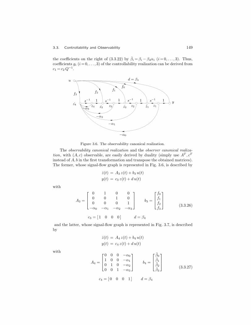
3.3. Controllability and Observability 149
the coefficients on the right of (3.3.22) by βi =βi−β4αi (i=0, . . . , 3). Thus,coefficients gi (i=0, . . . , 3) of the controllability realization can be derived fromc1 = c2Q
−1.
y1 1 1 1s−1 s−1 s−1 s−1
z4
u d = β4
f0f1f2f3
−α3
−α2
−α1
−α0
z1z1z2z2z3z3z4
Figure 3.6. The observability canonical realization.
The observability canonical realization and the observer canonical realiza-tion, with (A, c) observable, are easily derived by duality (simply use AT , cT
instead of A, b in the first transformation and transpose the obtained matrices).The former, whose signal-flow graph is represented in Fig. 3.6, is described by
z(t) = A3 z(t) + b3 u(t)
y(t) = c3 z(t) + d u(t)
with
A3 =
⎡⎢⎣
0 1 0 00 0 1 00 0 0 1−α0 −α1 −α2 −α3
⎤⎥⎦ b3 =
⎡⎢⎣f0f1f2f3
⎤⎥⎦
c3 = [ 1 0 0 0 ] d = β4
(3.3.26)
and the latter, whose signal-flow graph is represented in Fig. 3.7, is describedby
z(t) = A4 z(t) + b4 u(t)
y(t) = c4 z(t) + d u(t)
with
A4 =
⎡⎢⎣0 0 0 −α0
1 0 0 −α1
0 1 0 −α2
0 0 1 −α3
⎤⎥⎦ b4 =
⎡⎢⎣β0β1β2β3
⎤⎥⎦
c4 = [ 0 0 0 1 ] d = β4
(3.3.27)

150 Chapter 3. The Geometric Approach: Classic Foundations
y1 1 1 1s−1 s−1 s−1 s−1
z1
u d = β4
β3β2β1β0
−α3
−α2
−α1
−α0
z4z4z3z3z2z2z1
Figure 3.7. The observer canonical realization.
where βi =βi−β4αi (i=0, . . . , 3) are the same as in the controller canonicalrelization.
The identity of βi (i=0, . . . , 3) (the components of b4) with the correspond-ing βi’s on the left of (3.3.22) is proved again by using the Mason’s formula.Coefficients fi (i=0, . . . , 3) of the observer realization are consequently derivedfrom b3=Q−1b4.
3.3.4 Structural Indices and MIMO Canonical Forms
The concepts of controllability and controller canonical forms will now beextended to multi-input systems. Consider a controllable pair (A,B), whereA and B are assumed to be respectively n×n and n× p. We shall denoteby b1, . . . , bp the columns of B and by μ≤ p its rank. Vectors b1, . . . , bμ areassumed to be linearly independent. This does not imply any loss of generality,since, if not, inputs can be suitably renumbered. Consider the table
b1Ab1A2 b1. . .
b2 . . .A b2 . . .A2 b2 . . .
bμAbμA2 bμ
(3.3.28)
which is assumed to be constructed by rows: each column ends when a vector isobtained that can be expressed as a linear combination of all the previous ones.This vector is not included in the table and the corresponding column is notcontinued because, as will be shown herein, also all subsequent vectors wouldbe linear combinations of the previous ones. By the controllability assumption,a table with exactly n linearly independent elements is obtained. Denote byri (i=1, . . . , μ) the numbers of the elements of the i-th column: the abovecriterion to end columns implies that vector Ari bi is a linear combination of

3.3. Controllability and Observability 151
all previous ones, i.e.,
Ari bi = −μ∑
j=1
ri−1∑h=0
αijh Ah bj −
∑j<i
αijri Ari bj (i=1, . . . , μ) (3.3.29)
where the generic coefficient αijh is zero for h≥ rj . The following propertyholds.
Property 3.3.4 If Ari bi is a linear combination of the previous vectors intable (3.3.28), also Ari+k bi for all positive integers k, is a linear combinationof the previous vectors.
Proof. For k=1 the property is proved by multiplying on the right by A bothmembers of the i-th of (3.3.29) and by eliminating, in the sums at the rightside member, all vectors that, according to (3.3.29), can be expressed as linearcombinations of the previous ones, in particular Ari bi. The proof is extendedby induction to the case k > 1. �
Another interesting property of table (3.3.28) is the following.
Property 3.3.5 The set {ri (i=1, . . . , μ)} does not depend on the orderingassumed for columns of B in table (3.3.28).
Proof. The number of columns of table (3.3.28) with generic length i is equalto the integer Δρi−1 −Δρi, with
Δρi := ρ([B|AB| . . . |AiB])− ρ([B|AB| . . . |Ai−1 B])
which is clearly invariant with respect to permutations of columns of B. �
It is worth noting that, although the number of columns of table (3.3.28)with generic length i is invariant under a permutation of columns of B, thevalue of the ri’s corresponding to column bi may commute with each other.
Constants ri (i=1, . . . , μ) are called the input structural indices and rep-resent an important characterization of dynamic systems. The value of thegreatest input structural index is called the controllability index .
It is now possible to extend to multivariable systems the SISO canonicalforms and realizations described in Subsection 3.3.3. We shall consider only thecontrollability and the controller form, since the others, related to observability,can easily be derived by duality.
To maintain expounding at a reasonable level of simplicity we refer to aparticular case, corresponding to n=9, p=5, μ=3, in which table (3.3.28) isassumed to be
b1Ab1
b2Ab2A2 b2A3 b2
b3Ab3A2 b3
(3.3.30)

152 Chapter 3. The Geometric Approach: Classic Foundations
The input structural indices, presented in decreasing order, are in this case4, 3, 2, and the controllability index is 4. Relations (3.3.29) can be written as
A2b1 = −α110b1−α111Ab1−α120b2−α121Ab2−α130b3−α131Ab3
A4b2 = −α210b1−α211Ab1−α220b2−α221Ab2−α222A2b2−α223A
3b2 −α230b3−α231Ab3
A3b3 = −α310b1−α311Ab1−α320b2−α321Ab2−α322A2b2−α323A
3b2 −α330b3−α331Ab3 (3.3.31)
The controllability canonical form is obtained through the coordinate trans-formation defined by
T1 := [b1 |Ab1 |A2 b1 | b2 |Ab2 |A2 b2 |A3 b2 | b3 |Ab3 |A2 b3]
Matrices A1 :=T−11 AT1 and B1 :=T−11 B have the structures shown in(3.3.32, 3.3.33), as can easily be proved with arguments similar to the single-input case. Note that the submatrices on the main diagonal of A1 are incompanion form. In matrix B1, ε11, ε21, ε31 and ε12, ε22, ε32 denote, respectively,the components of b4 and b5 with respect to b1, b2, b3.
A1 =
⎡⎢⎢⎢⎢⎢⎢⎢⎢⎢⎢⎢⎢⎢⎢⎢⎢⎢⎣
0 −α110 0 0 0 −α210 0 0 −α310
1 −α111 0 0 0 −α211 0 0 −α311
0 −α120 0 0 0 −α220 0 0 −α320
0 −α121 1 0 0 −α221 0 0 −α321
0 0 0 1 0 −α222 0 0 −α322
0 0 0 0 1 −α223 0 0 −α323
0 −α130 0 0 0 −α230 0 0 −α330
0 −α131 0 0 0 −α231 1 0 −α331
0 0 0 0 0 −α232 0 1 −α332
⎤⎥⎥⎥⎥⎥⎥⎥⎥⎥⎥⎥⎥⎥⎥⎥⎥⎥⎦
(3.3.32)
B1 =
⎡⎢⎢⎢⎢⎢⎢⎢⎢⎢⎢⎢⎢⎢⎢⎢⎢⎢⎢⎣
1 0 0 ε11 ε12
0 0 0 0 0
0 1 0 ε21 ε22
0 0 0 0 0
0 0 0 0 0
0 0 0 0 0
0 0 1 ε31 ε32
0 0 0 0 0
0 0 0 0 0
⎤⎥⎥⎥⎥⎥⎥⎥⎥⎥⎥⎥⎥⎥⎥⎥⎥⎥⎥⎦
(3.3.33)

3.3. Controllability and Observability 153
We shall now extend the controller form to multi-input systems. First,write (3.3.29) as
Ari(bi +
∑j<i
αijri bj
)= −
μ∑j=1
ri−1∑h=0
αijh Ah bj (i=1, . . . , μ) (3.3.34)
By means of the assumption
b′i := bi +∑j<i
αijri bj (i=1, . . . , μ)
relations (3.3.34) can be put in the form
Ari b′i = −μ∑
j=1
ri−1∑h=0
βijh Ah b′j (i=1, . . . , μ) (3.3.35)
If vectors (3.3.28) are linearly independent, the vectors of the similar tableobtained from b′i (i=1, . . . , μ) are also so, since each one of them is expressedby the sum of a vector of (3.3.28) with a linear combination of the previousones. We assume vectors of the new table as a new basis. In the particularcase of (3.3.30) these are
b1, A b1, A2 b1, b2, A b2, A
2 b2, A3 b2, b
′3, A b
′3, A
2 b′3
with b′3 := b3 +α323b2. Matrices A′1 and B′1 that express A and B with respectto the new basis are obtained as A′1 =F−11 A1 F1, B
′1 =F−11 B1, with
F1 :=
⎡⎢⎢⎢⎢⎢⎢⎢⎢⎢⎢⎢⎢⎢⎢⎢⎢⎢⎣
1 0 0 0 0 0 0 0 0
0 1 0 0 0 0 0 0 0
0 0 1 0 0 0 α323 0 0
0 0 0 1 0 0 0 α323 0
0 0 0 0 1 0 0 0 α323
0 0 0 0 0 1 0 0 0
0 0 0 0 0 0 1 0 0
0 0 0 0 0 0 0 1 0
0 0 0 0 0 0 0 0 1
⎤⎥⎥⎥⎥⎥⎥⎥⎥⎥⎥⎥⎥⎥⎥⎥⎥⎥⎦
(3.3.36)

154 Chapter 3. The Geometric Approach: Classic Foundations
We obtain matrices having the structures
A′1 =
⎡⎢⎢⎢⎢⎢⎢⎢⎢⎢⎢⎢⎢⎢⎢⎢⎢⎢⎣
0 −β110 0 0 0 −β210 0 0 −β3101 −β111 0 0 0 −β211 0 0 −β311
0 −β120 0 0 0 −β220 0 0 −β3200 −β121 1 0 0 −β221 0 0 −β3210 0 0 1 0 −β222 0 0 −β3220 0 0 0 1 −β223 0 0 0
0 −β130 0 0 0 −β230 0 0 −β3300 −β131 0 0 0 −β231 1 0 −β3310 0 0 0 0 −β232 0 1 −β332
⎤⎥⎥⎥⎥⎥⎥⎥⎥⎥⎥⎥⎥⎥⎥⎥⎥⎥⎦
(3.3.37)
B′1 =
⎡⎢⎢⎢⎢⎢⎢⎢⎢⎢⎢⎢⎢⎢⎢⎢⎢⎢⎢⎣
1 0 0 ε′11 ε′12
0 0 0 0 0
0 1 −α323 ε′21 ε′22
0 0 0 0 0
0 0 0 0 0
0 0 0 0 0
0 0 1 ε′31 ε′32
0 0 0 0 0
0 0 0 0 0
⎤⎥⎥⎥⎥⎥⎥⎥⎥⎥⎥⎥⎥⎥⎥⎥⎥⎥⎥⎦
(3.3.38)
In (3.3.38) ε′11, ε′21, ε
′31 and ε′12, ε
′22, ε
′32 are the components of b4 and b5 with
respect to b′1, b′2, b′3. As the last step, express A and B with respect to the basis
q1 = Aq2 + β111 q2 + β211 q6 + β311 q9q2 = b′1 = b1q3 = Aq4 + β121 q2 + β221 q6 + β321 q9q4 = Aq5 + β222 q6 + β322 q9q5 = Aq6 + β223 q6 + β323 q9q6 = b′2 = b3q7 = Aq8 + β131 q2 + β231 q6 + β331 q9q8 = Aq9 + β232 q6 + β332 q9q9 = b′3
(3.3.39)

3.3. Controllability and Observability 155
The corresponding transformation T2 and the new matrices A2 =T−12 A′1 T2,B2 =T−12 B′1 are
T2 :=
⎡⎢⎢⎢⎢⎢⎢⎢⎢⎢⎢⎢⎢⎢⎢⎢⎢⎢⎣
β111 1 β211 0 0 0 β311 0 0
1 0 0 0 0 0 0 0 0
β121 0 β221 β222 β223 1 β321 β322 0
0 0 β222 β223 1 0 β322 0 0
0 0 β223 1 0 0 0 0 0
0 0 1 0 0 0 0 0 0
β131 0 β231 β232 0 0 β331 β332 1
0 0 β232 0 0 0 β332 0 0
0 0 0 0 0 0 1 0 0
⎤⎥⎥⎥⎥⎥⎥⎥⎥⎥⎥⎥⎥⎥⎥⎥⎥⎥⎦
(3.3.40)
A2 =⎡⎢⎢⎢⎢⎢⎢⎢⎢⎢⎢⎢⎢⎢⎢⎢⎢⎢⎢⎣
0 1 0 0 0 0 0 0 0
−β110 −β111 −β120 −β121 0 0 −β130 −β131 0
0 0 0 1 0 0 0 0 0
0 0 0 0 1 0 0 0 0
0 0 0 0 0 1 0 0 0
−β210 −β211 −β220 −β221 −β222 −β223 −β230 −β231 −β232
0 0 0 0 0 0 0 1 0
0 0 0 0 0 0 0 0 1
−β310 −β311 −β320 −β321 −β322 −β323 −β330 −β331 −β332
⎤⎥⎥⎥⎥⎥⎥⎥⎥⎥⎥⎥⎥⎥⎥⎥⎥⎥⎥⎦
(3.3.41)
B2 =
⎡⎢⎢⎢⎢⎢⎢⎢⎢⎢⎢⎢⎢⎢⎢⎢⎢⎢⎢⎢⎣
0 0 0 0 0
1 (−α214) (−α313) ε′11 ε′12
0 0 0 0 0
0 0 0 0 0
0 0 0 0 0
0 1 −α323 ε′21 ε′22
0 0 0 0 0
0 0 0 0 0
0 0 1 ε′31 ε′32
⎤⎥⎥⎥⎥⎥⎥⎥⎥⎥⎥⎥⎥⎥⎥⎥⎥⎥⎥⎥⎦
(3.3.42)

156 Chapter 3. The Geometric Approach: Classic Foundations
Vectors (3.3.39) are linearly independent since, considered in suitable order(i.e., in the reverse order in each chain), they can be obtained as the sum ofa vector of table (3.3.30) with a linear combination of the previous ones. Theelements in round brackets in (3.3.42) vanish in this particular case, but couldbe nonzero in the most general case.
The controllability canonical form and the controller canonical form arecanonical forms relative to input . By duality from pair (A,C) it is possible toderive the observability canonical form and the observer canonical form, alsocalled the canonical forms relative to output . The output structural indices canbe derived likewise. The value of the greatest output structural index is calledthe observability index of the system referred to.
3.4 State Feedback and Output Injection
The term feedback denotes an external connection through which the effects arebrought back to influence the corresponding causes. It is the main tool at thedisposal of designers to adapt system features to a given task, hence it is basicfor all synthesis procedures. In this section an important theorem concerningeigenvalues assignability will be stated and discussed. It directly relates con-trollability and observability with the possibility of arbitrarily assigning thesystem eigenvalues through a suitable feedback connection.
+
+
+
+
u
B
B
f
f
x = Ax+ f
x = Ax+ f
x
x
C
C
y
y
F
v
v
Σ
Σ
G
(a)
(b)
Figure 3.8. State feedback and output injection.
Refer to the triple (A,B,C) whose structure is represented in Fig. 3.1. In

3.4. State Feedback and Output Injection 157
Fig. 3.8 two basic feedback connections are shown: the state-to-input feedback ,often called simply state feedback , and the output-to-forcing action feedback ,also called output injection. In the former, the state is brought to act on theinput u through a purely algebraic linear connection, represented by the p×nreal matrix F , while in the latter the output is brought to act on forcing actionf again through a purely algebraic linear connection, represented by the n× qreal matrix G. The part shown in the dashed box in figures is the originalthree-map system Σ.
In actual physical systems neither connection is implementable, since nei-ther is the state accessible for direct measurement nor is the forcing actionaccessible for direct intervention. Nevertheless, these two schemes are use-ful to state some basic properties that will be referred to in the synthesis ofmore complex, but physically implementable, feedback connections, such as theoutput-to-input dynamic feedback, which will be examined later in this section.
We shall first refer to the standard state feedback connection, which isconsidered the basic one, since its properties are generally easily extensible tothe output injection by duality. The system represented in Fig. 3.8(a) has anew input v ∈Rp and is described by the equations
x(t) = (A+B F )x(t) +B v(t) (3.4.1)
y(t) = C x(t) (3.4.2)
in which matrix A has been replaced by A+BF . By a suitable choice of F anew system (3.4.1, 3.4.2) can be obtained with features significantly differentfrom those of the original one. One of these features is the spectrum of matrixA+BF , which can be completely assigned when pair (A,B) is controllable.The eigenvalue assignability theorem will be presented in two steps: first inrestricted form for SISO systems, then in the most general case of MIMOsystems.7
Theorem 3.4.1 (pole assignment: SISO systems) Refer to a SISO system(A, b, c). Let σ= {λ1, . . . , λn} be an arbitrary set of n complex numbers suchthat ρ∈σ implies ρ∗ ∈σ. There exists at least one row matrix f such that thespectrum of A+ bf coincides with σ if and only if (A, b) is controllable.
Proof. If. Let (A, b) be controllable. There exists a similarity transformationT such that A′ :=T−1AT and b′=T−1 b have the same structures as A2, b2 in(3.3.25). Parameters αi (i=0, . . . , n− 1) are the coefficients of the character-istic polynomial of A, which, in monic form, can in fact be written as
n−1∑i=0
αi λi + λn = 0
Let βi (i=0, . . . , n− 1) be the corresponding coefficients of the monic poly-nomial having the assigned eigenvalues as zeros; they are defined through the
7 The theorem on eigenvalue assignability is due to Langenhop [25] in the SISO case andWonham [38] in the MIMO case.

158 Chapter 3. The Geometric Approach: Classic Foundations
identityn−1∑i=0
βi λi + λn =
n∏i=1
(λ − λi)
Clearly the row matrix
f ′ := [α0− β0 |α1−β1 | . . . |αn−1−βn− 1]
is such that in the new basis A′+ b′f ′ has the elements of σ as eigenvalues.The corresponding matrix in the main basis
A+ b f with f := f ′ T−1
has the same eigenvalues, being similar to it.Only if. See the only if part of the MIMO case (Theorem 3.4.2). �
Theorem 3.4.2 (pole assignment: MIMO systems) Refer to a MIMO system(A,B,C). Let σ= {λ1, . . . , λn} be an arbitrary set of n complex numbers suchthat ρ∈σ implies ρ∗ ∈σ. There exists at least one p×n matrix F such thatthe spectrum of A+BF coincides with σ if and only if (A,B) is controllable.
Proof. If. For the sake of simplicity, a procedure for deriving a feedbackmatrix F that solves the pole assignment problem will be presented in theparticular case where pair (A,B) is transformed by T :=T2F1T1 into pair(A2, B2) whose structure is shown in (3.3.41, 3.3.42). The involved successivesimilarity transformations were derived in Subsection 3.3.4. We shall show thatby a suitable choice of the feedback matrix F it is possible to obtain for matrixB2FT , which represents BF in the new basis, the structure
B2 F T =
⎡⎢⎢⎢⎢⎢⎢⎢⎢⎢⎢⎢⎢⎢⎢⎢⎢⎢⎢⎣
0 0 0 0 0 0 0 0 0
× × × × × × × × ×
0 0 0 0 0 0 0 0 0
0 0 0 0 0 0 0 0 0
0 0 0 0 0 0 0 0 0
× × × × × × × × ×
0 0 0 0 0 0 0 0 0
0 0 0 0 0 0 0 0 0
× × × × × × × × ×
⎤⎥⎥⎥⎥⎥⎥⎥⎥⎥⎥⎥⎥⎥⎥⎥⎥⎥⎥⎦
(3.4.3)
where the elements denoted by × are arbitrary. Suppose, for a moment, thatthe last two columns of (3.3.42) are not present, i.e., that the system hasonly three inputs, corresponding to linearly independent forcing actions. It ispossible to decompose B2 as
B2 =M N (3.4.4)
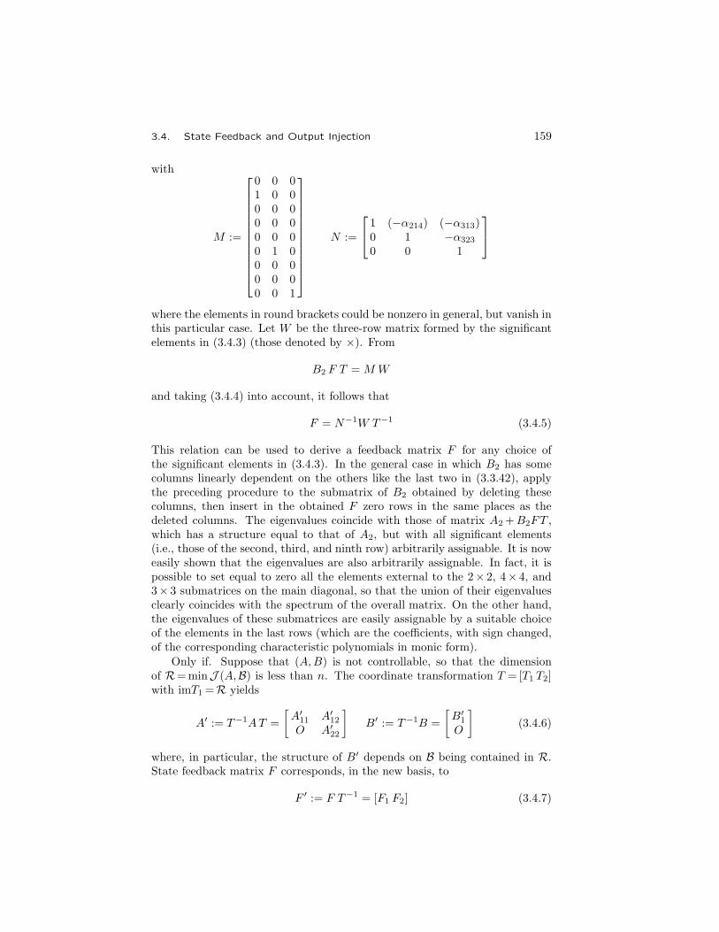
3.4. State Feedback and Output Injection 159
with
M :=
⎡⎢⎢⎢⎢⎢⎢⎢⎢⎢⎢⎢⎣
0 0 01 0 00 0 00 0 00 0 00 1 00 0 00 0 00 0 1
⎤⎥⎥⎥⎥⎥⎥⎥⎥⎥⎥⎥⎦
N :=
⎡⎣ 1 (−α214) (−α313)0 1 −α323
0 0 1
⎤⎦
where the elements in round brackets could be nonzero in general, but vanish inthis particular case. Let W be the three-row matrix formed by the significantelements in (3.4.3) (those denoted by ×). From
B2 F T =MW
and taking (3.4.4) into account, it follows that
F = N−1W T−1 (3.4.5)
This relation can be used to derive a feedback matrix F for any choice ofthe significant elements in (3.4.3). In the general case in which B2 has somecolumns linearly dependent on the others like the last two in (3.3.42), applythe preceding procedure to the submatrix of B2 obtained by deleting thesecolumns, then insert in the obtained F zero rows in the same places as thedeleted columns. The eigenvalues coincide with those of matrix A2 +B2FT ,which has a structure equal to that of A2, but with all significant elements(i.e., those of the second, third, and ninth row) arbitrarily assignable. It is noweasily shown that the eigenvalues are also arbitrarily assignable. In fact, it ispossible to set equal to zero all the elements external to the 2× 2, 4× 4, and3× 3 submatrices on the main diagonal, so that the union of their eigenvaluesclearly coincides with the spectrum of the overall matrix. On the other hand,the eigenvalues of these submatrices are easily assignable by a suitable choiceof the elements in the last rows (which are the coefficients, with sign changed,of the corresponding characteristic polynomials in monic form).
Only if. Suppose that (A,B) is not controllable, so that the dimensionof R=minJ (A,B) is less than n. The coordinate transformation T = [T1 T2]with imT1=R yields
A′ := T−1AT =
[A′11 A′12O A′22
]B′ := T−1B =
[B′1O
](3.4.6)
where, in particular, the structure of B′ depends on B being contained in R.State feedback matrix F corresponds, in the new basis, to
F ′ := F T−1 = [F1 F2] (3.4.7)
160 Chapter 3. The Geometric Approach: Classic Foundations
This influences only submatrices on the first row of A′, so that the eigenvaluesof A′22 cannot be varied. �
If there exists a state feedback matrix F such that A+BF is stable, thepair (A,B) is said to be stabilizable. Owing to Theorem 3.4.2 a completelycontrollable pair is always stabilizable. Nevertheless, the converse is not true:complete controllability is not necessary for (A,B) to be stabilizable, as thefollowing corollary states.
Corollary 3.4.1 Pair (A,B) is stabilizable if and only if R :=minJ (A,B) isexternally stable.
Proof. Refer to relations (3.4.6, 3.4.7) in the only if part of the proof ofTheorem 3.4.2: since (A′11, B
′1) is controllable, by a suitable choice of F ′1 it is
possible to obtain A′11 +B′1 F′1 having arbitrary eigenvalues, but it is impossible
to influence the second row of A′. Therefore, the stability of A′22 is necessaryand sufficient to make A′+B′F ′ (hence A+BF ) stable. �
Similar results concerning output injection are easily derived by duality.Refer to the system represented in Fig. 3.8(b), described by
x(t) = (A+GC)x(t) +B v(t) (3.4.8)
y(t) = C x(t) (3.4.9)
The more general result on pole assignment by state feedback (Theorem3.4.2) is dualized as follows.
Theorem 3.4.3 Refer to a MIMO system (A,B,C). Let σ= {λ1, . . . , λn} bean arbitrary set of n complex numbers such that ρ∈σ implies ρ∗ ∈σ. Thereexists at least one n× q matrix G such that the spectrum of A+GC coincideswith σ if and only if (A,C) is observable.
Proof. Since
maxJ (A, kerC) = {0} ⇔ minJ (AT , imCT ) = X
pair (A,C) is observable if and only if (AT , CT ) is controllable. In such a case,owing to Theorem 3.4.2 there exists at least one q×n matrix GT such thatthe spectrum of AT +CTGT coincides with the elements of σ. The statementfollows from the eigenvalues of any square matrix being equal to those of thetranspose matrix, which in this case is A+GC. �
If there exists an output injection matrix G such that A+GC is stable,pair (A,C) is said to be detectable. Owing to Theorem 3.4.3 an observablepair is always detectable. Nevertheless, the converse is not true: completeobservability is not necessary for (A,C) to be detectable, as stated by thefollowing corollary, which can easily be derived by duality from Corollary 3.4.1.

3.4. State Feedback and Output Injection 161
Corollary 3.4.2 Pair (A,C) is detectable if and only if Q :=maxJ (A, C) isinternally stable.
State feedback and output injection through eigenvalue variation influencestability. It is quite natural at this point to investigate whether they influenceother properties, as for instance controllability and observability themselves.We note that:
1. minJ (A,B)=minJ (A+BF,B) (state feedback does not influence control-lability);
2. maxJ (A, C)=maxJ (A+GC, C) (output injection does not influence ob-servability).
These properties can be proved in several ways. Referring to the former(the latter follows by duality), note that the feedback connection in Fig. 3.8(a)does not influence the class of the possible input functions u(·) (which, with orwithout feedback, is the class of all piecewise continuous functions with valuesin R
p), hence the reachable set. Otherwise refer to Algorithm 3.2.1 and notethat it provides a sequence of subspaces that does not change if A is replacedby A+BF . In fact, if this is the case, term BF Zi−1 is added on the rightof the definition formula of generic Zi: this term is contained in B, hence isalready a part of Zi.
On the other hand, state feedback can influence observability and outputinjection can influence controllability. For instance, by state feedback thegreatest (A,B)-controlled invariant (see next section) contained in C can betransformed into an (A+BF )-invariant. Since it is, in general, larger than Q,the unobservability subspace is extended.
Furthermore, feedback can make the structures of matrices A+BF andA+GC different from that of A, in the sense that the number and dimensionsof the Jordan blocks can be different. To investigate this point we shall referagain to the canonical forms, in particular to the proof of Theorem 3.4.2. First,consider the following lemma.
Lemma 3.4.1 A companion matrix has no linearly independent eigenvectorscorresponding to the same eigenvalue.
Proof. Consider the single-input controller form (A2, b2) defined in (3.3.20).Let λ1 be an eigenvalue of A2 and x=(x1, . . . , xn) a corresponding eigenvector,so that
(A2 − λ1I)x = 0
or, in detail
−λ1 x1 + x2 = 0
−λ1 x2 + x3 = 0
. . .
−λ1 xn−1 + xn = 0
−α0 x1 − α1 x2 − . . . − (αn−1 +λ1)xn = 0

162 Chapter 3. The Geometric Approach: Classic Foundations
These relations, considered as equations with x1, . . . , xn as unknowns, ad-mit a unique solution, which can be worked out, for instance, by setting x1 =1and deriving x2, . . . , xn from the first n− 1 equations. The last equation hasno meaning because, by substitution of the previous ones, it becomes
(α0 + α1λ1 + . . .+ αn−1λn1 )x1 = 0
which is an identity, since λ1 is a zero of the characteristic polynomial. �
This lemma is used to prove the following result, which points out theconnection between input structural indices and properties of the system matrixin the presence of state feedback.
Theorem 3.4.4 Let (A,B) be controllable. A suitable choice of F allows,besides the eigenvalues to be arbitrarily assigned, the degree of the minimalpolynomial of A+BF to be made equal, at least, to the controllability index of(A,B).8
Proof. The proof of Theorem 3.4.2 has shown that by a suitable choice of thefeedback matrix F a system matrix can be obtained in the block-companionform, i.e., with companion matrices on the main diagonal and the remainingelements equal to zero: the dimension of each matrix can be made equalto but not less than the value of the corresponding input structural index.The eigenvalues of these matrices can be arbitrarily assigned: if they are allmade equal to one another, owing to Lemma 3.4.1 a Jordan block of equaldimension corresponds to every companion matrix. Since multiplicity of aneigenvalue as a zero of the minimal polynomial coincides with the dimension ofthe corresponding greatest Jordan block (see the proof of Theorem 2.5.5), themultiplicity of the unique zero of the minimal polynomial is equal to the greatestinput structural index, i.e., to the controllability index. On the other hand, ifthe assigned eigenvalues were not equal to each other, the degree of the minimalpolynomial, which has all the eigenvalues as zeros, could not be less, since theeigenvalues of any companion matrix (hence of that with greatest dimension)have a multiplicity at least equal to the dimension of the corresponding Jordanblock in this matrix, which is unique owing to Lemma 3.4.1. In other words, inany case the degree of the minimal polynomial of a companion matrix is equalto its dimension. �
The theorem just presented is very useful for synthesis as a complementon “structure assignment” of Theorem 3.4.2 on pole assignment: in fact, itstates a lower bound on the eigenvalue multiplicity in the minimal polynomial.For instance, in the case of discrete-time systems, by a suitable state feedback(which sets all the eigenvalues to zero) the free motion can be made to converge
8 Recall that the controllability index is the minimal value of i such thatρ([B|AB| . . . |Ai B])=n, while the observability index is the minimal value of j such thatρ([CT |AT CT | . . . |(AT )j CT ])=n.

3.4. State Feedback and Output Injection 163
to zero in a finite time. The minimal achievable transient time is specified inthe following corollary.
Corollary 3.4.3 Let (A,B) be controllable. By a suitable choice of F , matrixA+BF can be made nilpotent of order equal, at least, to the controllabilityindex of (A,B).
Proof. Apply the procedure described in the proof of Theorem 3.4.4 to obtainan A+BF similar to a block companion matrix with all eigenvalues zero andwith blocks having dimensions equal to the values of the input structuralindices. This matrix coincides with the Jordan form: note that a Jordanblock corresponding to a zero eigenvalue is nilpotent of order equal to itsdimension. �
Theorem 3.4.4 and Corollary 3.4.3 are dualized as follows.
Theorem 3.4.5 Let (A,C) be observable. A suitable choice of G allows,besides the eigenvalues to be arbitrarily assigned, the degree of the minimalpolynomial of A+GC to be made equal, at least, to the observability index of(A,C).
Corollary 3.4.4 Let (A,C) be controllable. By a suitable choice of G, matrixA+GC can be made nilpotent of order equal, at least, to the observability indexof (A,C).
3.4.1 Asymptotic State Observers
Special dynamic devices, called asymptotic observers , are used to solve numer-ous synthesis problems.9 These are auxiliary linear time-invariant dynamicsystems that are connected to the input and output of the observed systemand provide an asymptotic estimate of its state, i.e., provide an output z thatasymptotically approaches the observed system state. In practice, after a cer-tain settling time from the initial time (at which the observer is connected tothe system), z(t) will reproduce the time evolution of the system state x(t).The asymptotic state observer theory is strictly connected to that of the eigen-value assignment presented earlier. In fact, for an asymptotic observer to berealized, a matrix G must exist such that A+GC is stable, i.e., pair (A,C)must be observable or, at least, detectable.
Consider a triple (A,B,C). If A is asymptotically stable (has all theeigenvalues with negative real part), a state asymptotic estimate z(t) (statereconstruction in real time) can be achieved by applying the same input signal
9 Although the word “observability” usually refers to the ability to derive the initial state,following the literature trend we shall indifferently call “observer” or “estimator” a specialdynamic device that provides an asymptotic estimate of the current state of a system towhose input and output it is permanently connected.

164 Chapter 3. The Geometric Approach: Classic Foundations
u x = Ax+B u
y = C x
y
z = Az +B uz
Figure 3.9. State estimate obtained through a model.
to a model of the system, i.e., another system, built “ad hoc,” with a state z(t)whose time evolution is described by the same matrix differential equation, i.e.
z(t) = Az(t) +B u(t) (3.4.10)
The corresponding connection is shown in Fig. 3.9. This solution has two maindrawbacks:
1. it is not feasible if the observed system is unstable;
2. it does not allow settling time to be influenced.
In fact, let e be the estimate error , defined by
e(t) := z(t)− x(t) (3.4.11)
Subtracting the system equation
x(t) = Ax(t) +B u(t) (3.4.12)
from (3.4.10) yieldse(t) = Ae(t)
from which it follows that the estimate error has a time evolution dependingonly on matrix A and converges to zero whatever its initial value is if and onlyif all the eigenvalues of A have negative real part.
A more general asymptotic observer, where both the above drawbacks canbe eliminated, is shown in Fig. 3.10. It is named identity observer and isdifferent from that shown in Fig. 3.9 because it also derives information fromthe system output. It is described by
z(t) = (A+GC) z(t) +B u(t)−Gy(t) (3.4.13)
Matrix G in (3.4.13) is arbitrary. The model of Fig. 3.9 can be derived as aparticular case by setting G=O. Subtracting (3.4.12) from (3.4.13) and using(3.4.11) yields the differential equation
e(t) = (A+GC) e(t) (3.4.14)
from which, owing to Corollary 3.4.2, it follows that if (A,C) is observable theconvergence of the estimate to the actual state can be made arbitrarily fast.These considerations lead to the following statement.

3.4. State Feedback and Output Injection 165
u x = Ax+B u
y = C x
y
z = (A+GC) z
+B u−Gy
z
Figure 3.10. State estimate obtained through an asymptotic observer.
Property 3.4.1 For any triple (A,B,C) with (A,C) observable there existsa state observer whose estimate error evolves in time as the solution of alinear, homogeneous, constant-coefficient differential equation of order n witharbitrarily assignable eigenvalues.
If (A,C) is not observable, a suitable choice of G can modify onlythe eigenvalues of A that are not internal to the unobservability subspaceQ :=maxJ (A, C): an asymptotic estimation of the state is possible if andonly if the system is detectable.
Asymptotic Observers and Complementability. We shall now showthat, under very general conditions, any stable dynamic system connected tothe output of a free system behaves as an asymptotic observer, because itprovides an asymptotic estimate of a linear function of the system state.10
Consider the free system
x(t) = Ax(t) (3.4.15)
y(t) = C x(t) (3.4.16)
and suppose a generic linear time-invariant dynamic system is connected to itsoutput. The time evolution of state z of this system is assumed to be describedby
z(t) = N z(t) +M y(t) (3.4.17)
with N stable. The problem is to state conditions under which there exists amatrix T such that
z(t) = T x(t) ∀ t> 0 (3.4.18)
if the initial conditions satisfy
z(0) = T x(0) (3.4.19)
From
z(t)− T x(t) = N z(t) +M C x(t) − T A x(t)
= (N T +M C − T A)x(t)10 The general theory of asymptotic observers, including these results, are due to Luen-
berger [28, 29, 31].

166 Chapter 3. The Geometric Approach: Classic Foundations
it follows that, because x(0) is generic, (3.4.18) holds if and only ifNT +MC −TA=0, i.e., if and only if T satisfies the Sylvester equation
N T − T A = −M C (3.4.20)
We recall that this equation has a unique solution T if and only if A andN have no common eigenvalues (Theorem 2.5.10). If (3.4.20) holds it followsthat
z(t)− T x(t) = N(z(t)− T x(t)
)Hence
z(t) = T x(t) + eNt(z(0)− T x(0)
)which means that, when initial condition (3.4.19) is not satisfied, (3.4.18) doesnot hold identically in time, but tends to be satisfied as t approaches infinity.
The obtained result is susceptible to geometric interpretation: by introduc-ing an extended state x, equations (3.4.15) and (3.4.17) can be written togetheras
˙x(t) = Ax(t)
where
x :=
[xz
]A :=
[A OMC N
]
In the extended state space X , the subspace
Z :={x : x = 0
}(the z coordinate hyperplane) is clearly an A-invariant: it corresponds to anasymptotic observer if and only if it is complementable.
If, instead of the free system (3.4.15, 3.4.16), we consider a system withforcing action B u(t), the asymptotic estimation of the same linear function ofstate can be obtained by applying a suitable linear function of input also tothe observer. In this case (3.4.17) is replaced by
z(t) = N z(t) +M y(t) + T B u(t) (3.4.21)
It may appear at this point that the identity observer, where
N := A+GC M = −G
with arbitraryG, is a very particular case. This is not true because any observerof order n providing a complete estimate of the state is equivalent to it (i.e.,has a state isomorphic to its state). In fact, let T be the corresponding matrixin (3.4.20) which, in this case, is nonsingular: from (3.4.20) it follows that
N = T AT−1 −M C T−1 = T (A− T−1M C)T−1 (3.4.22)
In the above arguments no assumption has been considered on systemobservability which, actually, is needed only as far as pole assignability of theobserver is concerned. Nevertheless, to obtain an asymptotic state estimate itis necessary that the observed system be detectable, since Q⊆ kerT for all Tsatisfying (3.4.20).
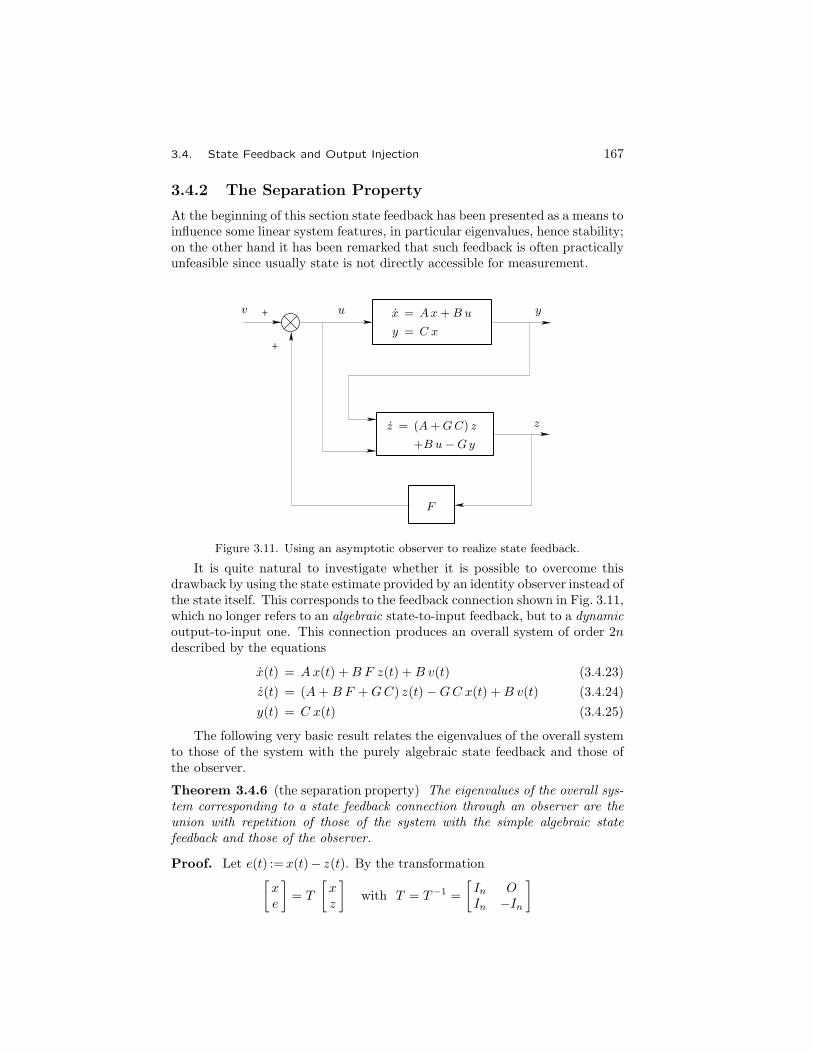
3.4. State Feedback and Output Injection 167
3.4.2 The Separation Property
At the beginning of this section state feedback has been presented as a means toinfluence some linear system features, in particular eigenvalues, hence stability;on the other hand it has been remarked that such feedback is often practicallyunfeasible since usually state is not directly accessible for measurement.
+
+
uv x = Ax+B u
y = C x
y
z = (A+GC) z
+B u−Gy
z
F
Figure 3.11. Using an asymptotic observer to realize state feedback.
It is quite natural to investigate whether it is possible to overcome thisdrawback by using the state estimate provided by an identity observer instead ofthe state itself. This corresponds to the feedback connection shown in Fig. 3.11,which no longer refers to an algebraic state-to-input feedback, but to a dynamicoutput-to-input one. This connection produces an overall system of order 2ndescribed by the equations
x(t) = Ax(t) +B F z(t) +B v(t) (3.4.23)
z(t) = (A+B F +GC) z(t)−GC x(t) +B v(t) (3.4.24)
y(t) = C x(t) (3.4.25)
The following very basic result relates the eigenvalues of the overall systemto those of the system with the purely algebraic state feedback and those ofthe observer.
Theorem 3.4.6 (the separation property) The eigenvalues of the overall sys-tem corresponding to a state feedback connection through an observer are theunion with repetition of those of the system with the simple algebraic statefeedback and those of the observer.
Proof. Let e(t) := x(t)− z(t). By the transformation[xe
]= T
[xz
]with T = T−1 =
[In OIn −In
]

168 Chapter 3. The Geometric Approach: Classic Foundations
from (3.4.23, 3.4.24) we derive[x(t)e(t)
]=
[A+B F −B F
O A+GC
] [x(t)e(t)
]+
[BO
]v(t) (3.4.26)
The spectrum of the system matrix in (3.4.26) is clearly σ(A+BF ) �σ(A+GC): it is equal to that of the original system (3.4.23, 3.4.24) from which(3.4.26) has been obtained by means of a similarity transformation. �
As a consequence of Theorems 3.4.2, 3.4.3, and 3.4.6, it follows that, ifthe triple (A,B,C) is completely controllable and completely observable, theeigenvalues of the overall system represented in Fig. 3.11 are all arbitrarilyassignable. In other words, any completely controllable and observable dynamicsystem of order n is stabilizable with an output-to-input dynamic feedback (or,simply, output dynamic feedback), i.e., through a suitable dynamic system, alsoof order n.
The duality between control and observation, a characteristic feature oflinear time-invariant systems, leads to the introduction of the so-called dualobservers or dynamic precompensators , which are also very important to char-acterize numerous control system synthesis procedures.
To introduce dynamic precompensators, it is convenient to refer to the blockdiagram represented in Fig. 3.12(a), which, like that in Fig. 3.9, represents theconnection of the observed system with a model; here in the model the purelyalgebraic operators have been represented as separated from the dynamic part,pointing out the three-map structure. The identity observer represented inFig. 3.10 is obtained through the connections shown in Fig. 3.12(b), in whichsignals obtained by applying the same linear transformationG to the outputs ofboth the model and the system are added to and subtracted from the forcingaction. These signals, of course, have no effect if the observer is trackingthe system, but influence time behavior and convergence to zero of a possibleestimate error.
The identity dynamic precompensator is, on the contrary, obtained byexecuting the connections shown in Fig. 3.12(c), from the model state to boththe model and system inputs. Also in this case, since contributions to inputsare identical, if the system and model states are equal at the initial time,their subsequent evolutions in time will also be equal. The overall system,represented in Fig. 3.12(c), is described by the equations
x(t) = Ax(t) +B F z(t) +B v(t) (3.4.27)
z(t) = (A+B F ) z(t) +B v(t) (3.4.28)
from which, by difference, it follows that
e(t) = Ae(t) (3.4.29)
If the triple (A,B,C) is asymptotically stable (this assumption is not veryrestrictive because, as previously shown, under complete controllability and

3.4. State Feedback and Output Injection 169
+
++
_
+
+
+
+
u
u
u
x = Ax+B u
y = C x
x = Ax+B u
y = C x
x = Ax+B u
y = C x
y
y
y
z = Az + ϕ
z = Az + ϕ
z = Az + ϕ
z
z
z
C
C
C
B
B
B
η
η
η
ϕ
ϕ
ϕ
G
G
F
F
v
(a)
(b)
(c)
Figure 3.12. Model, asymptotic observer and dynamic precompensator
(dual observer).

170 Chapter 3. The Geometric Approach: Classic Foundations
observability assumption eigenvalues are arbitrarily assignable by means of adynamic feedback), once the transient due to the possible difference in theinitial states is finished, system and precompensator states will be identical atevery instant of time. If the considered system is completely controllable, thedynamic behavior of the precompensator can be influenced through a suitablechoice of matrix F . For instance, an arbitrarily fast response can be obtainedby aptly assigning the eigenvalues of A+BF .
Note that the dynamic feedback shown in Fig. 3.11 can be obtained byperforming both connections of Fig. 3.12(b) (G blocks) and of Fig. 3.12(c)(F blocks): in the dynamic precompensator case it is equivalent to a purelyalgebraic feedback G from the output difference η− y to forcing action ϕ.
Extension to Discrete Systems. All the previous results on poleassignment, asymptotic state estimation, and the separation property can easilybe extended to discrete systems. A specific feature of these systems is thepossibility to extinguish the free motion in a finite number of transitions byassigning the value zero to all eigenvalues. This feature suggests alternativesolutions to some typical control problems. Two significant examples arereported in the following.
Problem 3.4.1 (control to the origin from a known initial state) Refer toa discrete pair (Ad, Bd), which is assumed to be controllable. Find a controlsequence u|[0,k] that causes the transition from an arbitrary initial state x(0) tothe origin in the minimal number of steps compatible with any initial state.11
Solution. Find a state feedback F such that Ad+BdF is nilpotent of orderequal to the controllability index of (Ad, Bd). This is possible owing to Corol-lary 3.4.3. Solution of the problem reduces to determination of the free motionof a discrete free system, i.e., to a simple iterative computation. �
Problem 3.4.2 (control to the origin from an unknown initial state) Refer toa discrete triple (Ad, Bd, Cd), which is assumed to be controllable and observ-able. Determine a control sequence u|[0,k] whose elements can be functions ofthe observed output, which causes the transition from an unknown initial stateto the origin.
Solution. Realize an output-to-input dynamic feedback (through a stateobserver) of the type shown in Fig. 3.11. From Theorem 3.4.6 and Corollaries3.4.3 and 3.4.4 it follows that by a suitable choice of F and G the overall systemmatrix can be made nilpotent of order equal to the sum of controllability andobservability indices, so that the number of steps necessary to reach the originis not greater than this sum. �
11 This problem was also solved in Subsection 2.6.2, but in the more general case of lineartime-varying discrete systems and with assigned control time.

3.5. Some Geometric Aspects of Optimal Control 171
3.5 Some Geometric Aspects of Optimal Con-
trol
In this section we shall present a geometric framework for dynamic optimizationproblems. Consider the linear time-varying system
x(t) = A(t)x(t) +B(t)u(t) (3.5.1)
where A(·) and B(·) are known, piecewise continuous real matrices, functions oftime. The state space is Rn and the input space Rm. We shall denote by [t0, t1]the optimal control time interval , i.e., the time interval to which the optimalcontrol problem is referred, by x0 :=x(t0) the initial state and by x1 := x(t1)the final state, or the extreme point of the optimal trajectory.
In many optimal control problems the control function is assumed to bebounded: for instance, it may be bounded in magnitude component by compo-nent, through the constraints
|uj(t)| ≤ H (j=1, . . . ,m) , t∈ [t0, t1] (3.5.2)
or, more generally, byu(t) ∈ Ω , t∈ [t0, t1] (3.5.3)
where Ω denotes a convex, closed, and bounded subset of Rp containing theorigin. Note that (3.3.2) expresses a constraint on the ∞-norm of controlfunction segment u[t0,t1]. Of course, different individual bounds on everycontrol component and unsymmetric bounds can be handled through suitablemanipulations of reference coordinates, such as translation of the origin andscaling.
In order to state an optimization problem a measure of control “goodness”is needed: this is usually expressed by a functional to be minimized, calledthe performance index . We shall here consider only two types of performanceindices: the linear function of the final state
Γ = 〈γ, x(t1)〉 (3.5.4)
where γ ∈Rn is a given vector, and the integral performance index
Γ =
∫ t1
t0
f(x(τ), u(τ), τ
)dτ (3.5.5)
where f is a continuous function, in most cases convex. In (3.5.4) and (3.5.5)symbol Γ stands for cost : optimization problems are usually formulated interms of achieving a minimum cost; of course, maximization problems arereduced to minimization ones by simply changing the sign of the functional.
In addition to the performance index, optimal control problems requiredefinition of an initial state set X0, and a final state set X1 (which may reduceto a single point or extend to the whole space). A typical dynamic optimization

172 Chapter 3. The Geometric Approach: Classic Foundations
problem consists of searching for an initial state x0 ∈X0 and an admissiblecontrol function u(·) such that the corresponding terminal state satisfies x1 ∈X1
and the performance index is minimal (with respect to all the other admissiblechoices of x0 and u(·)). The initial time t0 and/or the final time t1 are given apriori or must also be optimally derived.
isocost hyperplanes
X1
an admissibletrajectory
x1
an optimaltrajectory
x0
X0
W(t1)
γ
Figure 3.13. The geometric meaning of an optimization problem with
performance index defined as a linear function of the final state.
Fig. 3.13 shows a geometric interpretation of a dynamic optimization prob-lem with the performance index of the former type and fixed control timeinterval. W(t1) is the set of all states reachable at time t1 from event (x0, t0).Due to the superposition property, it can be expressed as
W(t1) := Φ(t1, t0)X0 +R+(t0, t1, 0) (3.5.6)
where
R+(t0, t1, 0) :={x1 : x1 =
∫ t1
t0
Φ(t1, τ)B(τ)u(τ) dτ , u(τ) ∈ Ω}
(3.5.7)
is the reachable set from the origin with bounded control. Note the layout ofthe isocost hyperplanes: the final state x1 of an optimal trajectory belongs tothe intersection of X1 and W(t1) and corresponds to a minimal cost.
3.5.1 Convex Sets and Convex Functions
In dealing with optimization in the presence of constraints, we need the con-cepts and some properties of convex sets and convex functions.12
12 Extended treatment of convexity is beyond the scope of this book, so we report only thebasic definitions and properties. Good references are the books by Eggleston [6] and Berge[2].
3.5. Some Geometric Aspects of Optimal Control 173
Refer to the vector space Rn with the standard euclidean norm induced bythe inner product. The concepts of subspace and linear variety are consideredin Appendix A; however, since in dealing with convexity special emphasis onorthogonality and topological properties is called for, it is convenient to use aslightly different notation, more suitable for the particular topic at hand.
Given an n× p matrix B having rank p, the set
M :={x : x = Bμ, μ ∈ R
p}
(3.5.8)
is a subspace or a through the origin, for which B is a basis matrix. In an innerproduct space an alternative way of defining a subspace is
M :={x : Ax = 0
}(3.5.9)
where A is an (n− p)×n matrix such that BTA=O, i.e., a basis matrix forkerBT = (imB)⊥.
Similarly, the “shifted” linear varietyMs := {x0}+M, parallel toM andpassing through x0, is defined as
Ms :={x : x = x0 +Bμ, μ ∈ R
p}
(3.5.10)
orMs :=
{x : A(x− x0) = 0
}(3.5.11)
Relations (3.5.8, 3.5.10) are said to define linear varieties in parametricform, (3.5.9, 3.5.11) in implicit form.
A particularization of (3.5.10) is the straight line through two points x0, x1:
L :={x : x = x0 + μ(x1− x0), μ ∈ R
}(3.5.12)
while a particularization of (3.5.11) is the hyperplane with normal a passingthrough x0:
P :={x : 〈a, (x− x0)〉 = 0
}(3.5.13)
The hyperplane through n points x0, . . . , xn− 1 ∈Rn, such thatB := {x1−x0, . . . , xn− 1−x0} is a linearly independent set, is defined as
P :={x : x = x0 +Bμ, μ ∈ R
n−1 }where B is the n× (n− 1) matrix having the elements of B as columns.
The line segment joining any two points x1, x2 ∈Rn is defined by
R(x1, x2) :={x : x = x1 + μ(x2−x1), 0≤μ≤ 1
}(3.5.14)
The sets
H+(P) :={x : 〈a, (x− x0)〉 ≥ 0
}(3.5.15)
H−(P) :={x : 〈a, (x− x0)〉 ≤ 0
}(3.5.16)
are called closed half-spaces bounded by P , the hyperplane defined in (3.5.13),while the corresponding sets without the equality sign in the definition arecalled open half-spaces bounded by P and denoted by H+(P), H−(P).
174 Chapter 3. The Geometric Approach: Classic Foundations
Definition 3.5.1 (convex set) A set X ⊆Rn is said to be convex if for anytwo points x1, x2 ∈X the straight line segment joining x1 and x2 is containedin X . In formula, αx1 +(1−α)x2 ∈X for all x1, x2 ∈X and all α∈ [0, 1].
The following properties of convex sets are easily derived:
1. the intersection of two convex sets is a convex set;
2. the sum or, more generally, any linear combination of two convex sets is aconvex set;13
3. the cartesian product of two convex sets is a convex set;
4. the image of a convex set in a linear map is a convex set.
Since Rn is metric with the norm induced by the inner product, it is possibleto divide the points of any given set X ⊆Rn into interior, limit, and isolatedpoints according to Definitions A.6.5, A.6.6, and A.6.7. Clearly, a convex setcannot have any isolated point.
Definition 3.5.2 (dimension of a convex set) The dimension of a con-vex set X is the largest integer m for which there exist m+1 points xi ∈X(i=0, . . . ,m) such that the m vectors x1−x0, . . . , xm−x0 are linearly inde-pendent.
A convex set of dimension m is contained in the linear varietyM := {x0}+Bμ, μ∈Rn, whose basis matrix B has the above m vectors ascolumns. A convex set whose interior is not empty has dimension n.
Given a convex set X of dimension m, with m<n, it is possible to definethe relative interior of X (denoted by rintX ) as the set of all interior points ofX considered in the linear varietyM, i.e., referring to an m-dimensional vectorspace.
Definition 3.5.3 (support hyperplane of a convex set) A hyperplane P thatintersects the closure of a convex set X and such that there are no points of Xin one of the open half-spaces bounded by P is called a support hyperplane ofX . In other words, let x0 be a frontier point of X : P defined in (3.5.13) is asupport hyperplane of X at x0 if X ⊆H+(P) or X ⊆H−(P), i.e.
〈a, (x− x0)〉 ≥ 0 or 〈a, (x− x0)〉 ≤ 0 ∀x∈X (3.5.17)
When considering a particular support hyperplane, it is customary to refer tothe outer normal, i.e., to take the sign of a in such a way that the latter of(3.5.17) holds.
13 Given any two sets X ,Y ⊆Rn, their linear combination with coefficients α, β is definedas
αX + βY :={z : z = αx+ βy, x∈X , y ∈Y
}

3.5. Some Geometric Aspects of Optimal Control 175
Property 3.5.1 Any convex set X admits at least one support hyperplane Pthrough every point x0 of its boundary. Conversely, if through every boundarypoint of X there exists a support hyperplane of X , X is convex.
Hence, any convex set is the envelope of all its support hyperplanes.
Definition 3.5.4 (cone) A cone with vertex in the origin is a set C such thatfor all x∈C the half-line or ray αx, α≥ 0, is contained in C. A cone withvertex in x0 is a set C such that for all x∈C the ray x0 +α(x− x0), α≥ 0, iscontained in C.
Definition 3.5.5 (polar cone of a convex set) Let x0 be any point of theconvex set X . The polar cone of X at x0 (which will be denoted by Cp(X −x0))is defined as
Cp(X −x0) :={p : 〈p, (x− x0)〉 ≤ 0 ∀x∈X
}(3.5.18)
If x0 is a boundary point of X , Cp(X −x0) is the locus of the outer normalsof all the support hyperplanes of X at x0. If dimX =n and x0 is an interiorpoint of X , Cp(X −x0) clearly reduces to the origin. It is easy to prove thatany polar cone of a convex set is convex.
Definition 3.5.6 (convex function) A function f : D→R, where D denotesa convex subset of Rn, is said to be a convex function if for any two pointsx1, x2 ∈D and any α∈ [0, 1]
f(αx1 + (1−α)x2
)≤ αf(x1) + (1−α)f(x2) (3.5.19)
If the preceding relation holds with the strict inequality sign, function f issaid to be strictly convex ; if f is a (strictly) convex function, −f is said to be(strictly) concave.
f(x)
αf(x1) + (1− α)f(x2)
f (αx1 + (1− α)x2)
0 x1 x2 x
Figure 3.14. A convex function with D⊆R.
For example, in Fig. 3.14 the graph of a possible convex function withdomain in R is represented and the meaning of condition (3.5.19) is pointedout: note that the function cannot be constant on any finite segment of itsdomain if the value at some other point is less.

176 Chapter 3. The Geometric Approach: Classic Foundations
Property 3.5.2 The sum or, more generally, any linear combination withnonnegative coefficients of two convex functions is a convex function.
Proof. Let f, g be two convex functions with the same domain D andϕ := βf + γg with β, γ≥ 0 a linear combination of them. It follows that
ϕ(αx1 + (1−α)x2
)= β f
(αx1 + (1−α)x2
)+ γ g
(αx1 + (1−α)x2
)≤ αβ f(x1) + (1−α)β f(x2) + αγ g(x1) + (1−α)γ g(x2)
= αϕ(x1) + (1−α)ϕ(x2) �
It is easy to prove that a linear combination with positive coefficients oftwo convex functions is strictly convex if at least one of them is so.
Property 3.5.3 Let f be a convex function with a sufficiently large domainand k any real number. The set
X1 :={x : f(x) ≤ k
}is convex or empty.
Proof. Let x1, x2 ∈X1 and k1 := f(x1), k2 := f(x2). Then f(αx1 +(1−α)x2)≤αf(x1)+ (1−α)f(x2)=αk1 +(1−α)k2≤ k. �
Property 3.5.4 A positive semidefinite (positive definite) quadratic form isa convex (strictly convex) function.
Proof. Let f(x) := 〈x,Ax〉: by assumption f(x)> 0 (f(x)≥ 0) for all x �=0.Hence
αf(x1) + (1−α)f(x2) = α〈x1, Ax1〉+ (1−α)〈x2, Ax2〉f(αx1 + (1−α)x2
)= α2〈x1, Ax1〉+ 2α(1−α)〈x1, Ax2〉+ (1−α)2〈x2, Ax2〉
By subtraction on the right one obtains
α(1−α)〈x1, Ax1〉 − 2α(1−α)〈x1, Ax2〉+ α(1−α)〈x2, Ax2〉= α(1−α)〈(x1 −x2), A(x1−x2)〉 > 0 (≥ 0) ∀ x1, x2, x1 �=x2
Since the same inequality must hold for the difference of the left, the propertyis proved. �
Property 3.5.5 Let f be a continuously differentiable function defined on aconvex domain and x0 any point of this domain. Denote by
g(x0) := gradf |x0
the gradient of f at x0. Then f is convex if and only if
f(x) ≥ f(x0) + 〈g(x0), (x− x0)〉 (3.5.20)
In other words, a function is convex if and only if it is greater than or equal toall its local linear approximations.
3.5. Some Geometric Aspects of Optimal Control 177
Proof. Only if. From
f(x0 + α(x− x0)
)= f
(αx + (1−α)x0
)≤ αf(x) + (1−α)f(x0) (3.5.21)
it follows that
f(x) ≥ f(x0) +f(x0 +α(x− x0)
)− f(x0)
α
which converges to (3.5.20) as α approaches zero from the right.If. Consider any two points x1, x2 in the domain of f and for any α,
0≤α≤ 1, define x0 :=αx1 + (1−α)x2. Multiply relation (3.5.20) with x :=x1by α and with x := x2 by 1−α and sum: it follows that
αf(x1) + (1−α)f(x2) ≥ f(x0) + 〈g(x0),(αx1 +(1−α)x2− x0
)〉
= f(αx1 + (1−α)x2
)�
3.5.2 The Pontryagin Maximum Principle
The maximum principle is a contribution to the calculus of variations developedby the Russian mathematician L.S. Pontryagin to solve variational problems inthe presence of constraints on the control effort.14 It can be simply and clearlyinterpreted geometrically, especially in particular cases of linear systems withperformance index (3.5.4) or (3.5.5). We shall present it here referring only tothese cases.
Property 3.5.6 The reachable set R+(t0, t1, 0) of system (3.5.1) with controlfunction u(·) subject to constraint (3.5.3) is convex.
Proof. Let x1, x2 be any two terminal states belonging to R+(t0, t1, 0),corresponding to the admissible control functions u1(·), u2(·). Since u(t) isconstrained to belong to a convex set for all t∈ [t0, t1], also αu1(·)+(1−α)u2(·)is admissible, so that the corresponding terminal state αx1+(1−α)x2 belongsto R+(t0, t1, 0). �
Remark. Refer to Fig. 3.13: if the initial and final state sets X0,X1 areconvex, the set of all admissible x(t1) is still convex, it being obtained throughlinear transformations, sums, and intersections of convex sets.
It is easily shown that for any finite control interval [t0, t1] the reachable setR+(t0, t1, 0) is also closed, bounded, and symmetric with respect to the originif Ω is so.
Theorem 3.5.1 (the maximum principle, part I) Consider system (3.5.1)in a given control interval [t0, t1] with initial state x0, constraint (3.5.3) onthe control effort, and performance index (3.5.4). A state trajectory x(·) with
14 See the basic book by Pontryagin, Boltyanskii, Gamkrelidze, and Mishchenko [33].

178 Chapter 3. The Geometric Approach: Classic Foundations
initial state x(t0)= x0, corresponding to an admissible control function u(·), isoptimal if and only if the solution p(t) of the adjoint system
p(t) = −AT (t) p(t) (3.5.22)
with final condition p(t1) := − γ, satisfies the maximum condition15
〈p(t), B(t) (u− u(t))〉 ≤ 0 ∀u ∈ Ω a.e. in [t0, t1] (3.5.23)
Variable p is usually called the adjoint variable.
Proof. If. Let u(·) be another admissible control function and x(·) thecorresponding state trajectory. By difference we derive
〈p(t1), (x(t1)− x(t1))〉 = 〈p(t1),∫ t1
t0
Φ(t1, τ )B(τ )(u(τ )− u(τ )) dτ 〉
=
∫ t1
t0
〈ΦT (t1, τ ) p(t1) , B(τ )(u(τ )− u(τ ))〉 dτ
=
∫ t1
t0
〈p(τ ) , B(τ )(u(τ )− u(τ ))〉 dτ
Condition (3.5.23) implies that the inner product under the integral sign onthe right is nonpositive for all t∈ [t0, t1], so that the inner product on the left isalso nonpositive. Since p(t1)= − γ, any admissible variation of the trajectorycorresponds to a nonnegative variation of the cost, hence x(·) is optimal.
Only if. Suppose there exists a subset T ⊆ [t0, t1] with nonzero measuresuch that (3.5.23) does not hold for all t∈T : then it is possible to choose anadmissible control function u(·) (possibly different from u(·) only in T ) suchthat the corresponding state trajectory x(·) satisfies 〈p(t1), (x(t1)− x(t1))〉> 0or 〈γ, (x(t1)− x(t1))〉< 0, so that x(·) is nonoptimal. �
A Geometric Interpretation. The maximum principle can be interpretedin strict geometric terms as a necessary and sufficient condition for a givenvector ϕ to belong to the polar cone of the reachable set at some boundary pointx(t1). It can be used to derive the reachable set as an envelope of hyperplanes(see Example 3.5.1).
Refer to Fig. 3.15, where R denotes the (convex) reachable set of system(3.5.1) from the initial state x0, in the time interval [t0, t1], with the control
15 Some particular terms, which derive from the classical calculus of variations, are oftenused in optimal control theory. Function H(p, x, u, t) := 〈p, (A(t) x+B(t) u)〉 is called theHamiltonian function and the overall system (3.5.1, 3.5.22), consisting of the controlledsystem and adjoint system equations, is called the Hamiltonian system. It can be derived interms of the Hamiltonian function as
x(t) =∂H
∂p, p(t) = −∂H
∂x
The maximum condition requires the Hamiltonian function to be maximal at the optimalcontrol u(t) with respect to any other admissible control action u∈Ω at every instant oftime.

3.5. Some Geometric Aspects of Optimal Control 179
p(t0)
x(t0)=x0
p(t)
x(t)δx(t)
BT(u− u(t)
)
p(t1)=ϕ= − γ
x(t1)
δx(t1)
R
Figure 3.15. A geometric interpretation of the maximum principle: case
in which cost Γ is defined as a linear function of the final state.
effort constrained by (3.5.3). Recall that the inner product of a solution of thefree system
x(t) = A(t)x(t) (3.5.24)
and a solution of the adjoint system (3.5.22) is a constant (Property 2.1.3):since any variation δx(t) of trajectory x(·) at time t (due to an admissiblepulse variation of the control function) is translated at the final time t1 asδx(t1)=Φ(t1, t) δx(t), the inner product 〈p(t1), δx(t1)〉 is nonpositive (so thatp(t1) is the outer normal of a support hyperplane of R at x(t1)) if and only ifp(t) belongs to the polar cone of B(t)(Ω− u(t)) almost everywhere in [t0, t1].These remarks lead to the following statement.
Corollary 3.5.1 Let R be the reachable set of system (3.5.1) under the con-straints stated in Theorem 3.5.1. Denote by x(·), u(·) an admissible state tra-jectory and the corresponding control function. For any given vector ϕ∈Rn
relation
ϕ ∈ Cp(R− x(t1)
)(3.5.25)
holds if and only if
p(t) ∈ Cp(B(t) (Ω− u(t))
)a.e. in [t0, t1] (3.5.26)
with
p(t) = −AT (t) p(t) , p(t1) = ϕ (3.5.27)
which is equivalent to the maximum condition expressed by (3.5.23).

180 Chapter 3. The Geometric Approach: Classic Foundations
Theorem 3.5.1 allows immediate solution of a class of optimization prob-lems: refer to system (3.5.1) with control function subject to constraints (3.5.2),the initial state x0, and the control interval [t0, t1] given, the final state free andperformance index (3.5.4). Assume that the system is completely controllable.
Algorithm 3.5.1 An extremal trajectory of system (3.5.1) from initial statex0 at a given time t0 with control action subject to saturation constraints(3.5.2), corresponding to a minimum of cost (3.5.4) (where time t1 is givenand the final state is completely free), is determined as follows:
1. Solve the adjoint system (3.5.22) with p(t1) := − γ, i.e., computep(t)=ΦT (t1, t)p(t1), where Φ(·, ·) is the state transition matrix of homogeneoussystem (3.5.24);
2. Determine the optimal control function by means of the maximum conditionas
uj(t) = H sign(BT p(t)
)(j=1, . . . ,m) , t∈ [t0, t1] (3.5.28)
Note that the control function is of the so-called bang-bang type: everycomponent switches from one to the other of its extremal values. If theargument of function sign is zero for a finite time interval, the correspondingvalue of uj is immaterial: the reachable set has more than one point in commonwith its support hyperplane, so that the optimal trajectory is not unique.
Also note that both the adjoint system and the maximum condition arehomogeneous in p(·), so that scaling γ and p(·) by an arbitrary positive factordoes not change the solution of the optimal control problem.
We shall now derive the maximum principle for the case of integral per-formance index (3.5.5). Let us extend the state space by adding to (3.5.1) thenonlinear differential equation
c(t) = f(x(t), u(t), t
), c(t0) = 0 (3.5.29)
where f , the function appearing in (3.5.5), is assumed to be convex. Denote byx=(c, x) the extended state: by using this artifice we still have the performanceindex expressed as a linear function of the (extended) terminal state, sinceclearly
Γ = c(t1) = 〈e0, x(t1)〉 (3.5.30)
where e0 denotes the unit vector in the direction of c axis. Let R⊆Rn+1 be thereachable set in the extended state space. The standard reachable set R⊆Rn
is related to it byR =
{x : (c, x) ∈ R
}(3.5.31)
In order to extend the above stated maximum principle to the case at hand,the following definition is needed.
Definition 3.5.7 (directionally convex set) Let z be any vector of Rn. Aset X ⊆Rn is said to be z-directionally convex 16 if for any x1, x2 ∈X and any
16Directional convexity was introduced by Holtzmann and Halkin [12].

3.5. Some Geometric Aspects of Optimal Control 181
α∈ [0, 1] there exists a β≥ 0 such that αx1 + (1−α)x2 +βz ∈X . A point x0is a z-directional boundary point of X if it is a boundary point of X and allx0 +βz, β≥ 0, do not belong to X . If set X is z-directionally convex, the set
Xs :={y : y = x− βz , x∈X , β≥ 0
}(3.5.32)
which is called z-shadow of X , is convex.
Property 3.5.7 R+(t0, t1, 0), the reachable set of the extended system(3.5.29, 3.5.1) with control function u(·) subject to constraint (3.5.3), is (−e0)-directionally convex.
Proof. Let u1(·), u2(·) be any two admissible control functions and x1(·), x2(·)the corresponding extended state trajectories. Apply the control functionu(·) :=αu1(·) + (1−α)u2(·): the corresponding trajectory x(·) is such that
c(t1) =
∫ t1
t0
f(αx1(τ )+ (1−α)x2(τ ), αu1(τ )+ (1−α)u2(τ ), τ
)dτ
≤ α
∫ t1
t0
f(x1(τ ), u1(τ ), τ
)dτ + (1−α)
∫ t1
t0
f(x2(τ ), u2(τ ), τ
)dτ
= α c1(t1) + (1−α) c2(t1)
Hence
c(t1) = α c1(t1) + (1−α) c2(t1)− β , β ≥ 0 �
Theorem 3.5.2 (the maximum principle, part II) Consider system (3.5.1)in a given control interval [t0, t1] with initial state x0, constraint (3.5.3) on thecontrol effort, and performance index (3.5.5), where function f is assumed tobe convex. A state trajectory x(·) with initial state x(t0)= x0 and a given finalstate x(t1) strictly internal to the reachable set R is optimal if and only if forany real constant ψ< 0 there exists a solution p(·) of the adjoint system
p(t) = −AT (t) p(t)− ψ gradx f∣∣∣ x(t)u(t)
(3.5.33)
which satisfies the maximum condition
〈p(t), B(t) (u− u(t))〉+ ψ(f(x(t), u, t
)− f
(x(t), u(t), t
))≤ 0
∀u ∈ Ω a.e. in [t0, t1] (3.5.34)
Proof. Only if. Apply Theorem 3.5.1 locally (in a small neighborhoodof trajectory c(·), x(·) in the extended state space). For a trajectory to beoptimal the necessary conditions for the linear case must be satisfied for the firstvariation: in fact, if not, there would exist a small, admissible control functionvariation causing decrease in cost. The extended adjoint system corresponding

182 Chapter 3. The Geometric Approach: Classic Foundations
c
Rs
R x(t1)
P
p(t1)
ψ(t1)p(t1)
x
Figure 3.16. The reachable set in the extended state space: case in
which cost Γ is defined as the integral of a convex functional of the
state and control trajectories.
to local linearization of (3.5.29, 3.5.1) defines the extended adjoint variablep=(ψ, p), where ψ(·) satisfies the differential equation
ψ(t) = 0 (3.5.35)
and p(·) satisfies (3.5.33). In (3.5.35) the right side member is zero becausevariable c does not appear in the Jacobian matrix of (3.5.29, 3.5.1). Equation(3.5.35) implies that ψ(·) is constant over [t0, t1]. At an optimal terminal point¯x(t1), which is a (−e0)-directional boundary point of the extended reachableset R (see Fig. 3.16), a support hyperplane P of Rs has the outer normal withnegative component in the direction of axis c, so that constant ψ is negative:furthermore, it is arbitrary because all conditions are homogeneous in p(·). The“local” maximum condition
〈p(t), B(t) (u− u(t))〉 + ψ 〈gradu f∣∣∣ x(t)u(t)
, (u− u(t))〉 ≤ 0
∀u ∈ Ω a.e. in [t0, t1] (3.5.36)
is equivalent to (3.5.34) by virtue of Property 3.5.5.If. Due to convexity of f , any finite variation of the control function and
trajectory with respect to u(·) and x(·) (with δx(t1)= 0 since the terminalstate is given) will cause a nonnegative variation δc(t1) of the performanceindex. Thus, if the stated conditions are satisfied, P is a support hyperplaneof Rs. �

3.5. Some Geometric Aspects of Optimal Control 183
We consider now some computational aspects of dynamic optimizationproblems. Cases in which solution is achievable by direct computation, with-out any trial-and-error search procedure, are relatively rare. Algorithm 3.5.1refers to one of these cases: direct solution is possible because the final statehas been assumed completely free. However, when the final state is given,as in the case of Theorem 3.5.2, we have a typical two-point boundary valueproblem: it is solved by assuming, for instance, ψ := − 1 and adjusting p(t0),both in direction and magnitude, until the state trajectory, obtained by solvingtogether (3.5.1) and (3.5.33) with initial conditions x(t0) := x0, p(t0) and withthe control function provided at every instant of time by the maximum condi-tion (3.5.34) or (3.5.36), reaches x1 at time t1. Two particular optimal controlproblems that can be solved with this procedure are the minimum-time controland the minimum-energy control , which are briefly discussed hereafter. In bothcases system (3.5.1) is assumed to be completely controllable in a sufficientlylarge time interval starting at t0.
Problem 3.5.1 (minimum-time control) Consider system (3.5.1) with initialstate zero, initial time t0, final state x1 and constraint (3.5.3) on the controlaction. Derive a control function u(·) which produces transition from the originto x1 in minimum time.
Solution. Denote, as before, by R+(t0, t1, 0) the reachable set of (3.5.1)under constraint (3.5.3). Since Ω contains the origin
R+(t0, t1, 0) ⊆ R+(t0, t2, 0) for t1 < t2 (3.5.37)
In fact a generic point x′ of R+(t0, t1, 0), reachable at t1 by applying somecontrol function u′(·), can also be reached at t2 by
u′′(t) =
{0 for 0 ≤ t < t2− t1u′(t+ t2− t1) for t2− t1 ≤ t ≤ t2 (3.5.38)
In most cases (3.5.37) is a strict inclusion and, since R+(t0, t1, 0) is closed forany finite control interval, all its boundary points are reachable at minimaltime t1. The boundary is called an isochronous surface (corresponding totime t1). The problem is solved by searching (by a trial-and-error or steepestdescent procedure) for a value of p(t0) (only direction has to be varied, sincemagnitude has no influence) such that the simultaneous solution of (3.5.1) and(3.5.22) with control action u(t) chosen at every instant of time to maximize〈p(t), B(t)u(t)〉 over Ω, provides a state trajectory passing through x1: thecorresponding time t1 is the minimal time. This means that x1 belongs to theboundary of R+(t0, t1, 0) and the corresponding p(t1) is the outer normal ofa support hyperplane of R+(t0, t1, 0) at x1. The same procedure, based ontrial-and-error search for p(t0), can also be used for any given initial state x0(not necessarily coinciding with the origin). If the control action is constrainedby (3.5.2) instead of (3.5.3), u(·) is of the bang-bang type and is given by (28)at every instant of time as a function of p(t). �

184 Chapter 3. The Geometric Approach: Classic Foundations
-3
-2
-1
0
1
2
3
-4 -3 -2 -1 0 1 2 3 4
Figure 3.17. The reachable set R+(0, 2, 0) of system (3.5.39).
Example 3.5.1 Consider the linear time-invariant system corresponding to
A :=
[0 10 0
]B :=
[01
](3.5.39)
in the control interval [0, 2] and with the control effort constrained by−1≤u≤ 1. The boundary of R+(0, 2, 1), i.e., the isochronous curve for t1 =2,is represented in Fig. 3-19: it has been obtained by connecting 50 terminalpoints, each of which has been computed by applying Algorithm 3.5.1 to oneof 50 equally angularly spaced unit vectors pi(t1) :=ϕi (i=1, . . . , 50). Thecorresponding control actions, of the bang-bang type, are
ui(t) = sign(BT pi(t)
)with pi(t) = eA
T t ϕi (i=1, . . . , 50) (3.5.40)
Fig. 3.18 shows four different isochronous curves obtained with this procedure.
Problem 3.5.2 (minimum energy control) Consider system (3.5.1) with ini-tial state x0, initial time t0, final state x1, and control interval [t0, t1]. Derivea control function u(·) that produces transition from x0 to x1 with minimumenergy. Energy is defined as
e =
(∫ t1
t0
‖u(τ)‖22 dτ) 1
2
(3.5.41)
i.e., as the euclidean norm of control function segment u|[t0,t1].
Solution. By virtue of Property 3.5.4 functional (3.5.41) is convex and theproblem can be solved by applying Theorem 3.5.2 with Γ := e2/2. First, note
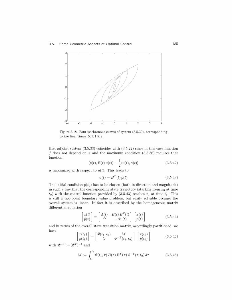
3.5. Some Geometric Aspects of Optimal Control 185
-3
-2
-1
0
1
2
3
-4 -3 -2 -1 0 1 2 3 4
Figure 3.18. Four isochronous curves of system (3.5.39), corresponding
to the final times .5, 1, 1.5, 2.
that adjoint system (3.5.33) coincides with (3.5.22) since in this case functionf does not depend on x and the maximum condition (3.5.36) requires thatfunction
〈p(t), B(t)u(t)〉 − 1
2〈u(t), u(t)〉 (3.5.42)
is maximized with respect to u(t). This leads to
u(t) = BT (t) p(t) (3.5.43)
The initial condition p(t0) has to be chosen (both in direction and magnitude)in such a way that the corresponding state trajectory (starting from x0 at timet0) with the control function provided by (3.5.43) reaches x1 at time t1. Thisis still a two-point boundary value problem, but easily solvable because theoverall system is linear. In fact it is described by the homogeneous matrixdifferential equation[
x(t)p(t)
]=
[A(t) B(t)BT (t)O −AT (t)
] [x(t)p(t)
](3.5.44)
and in terms of the overall state transition matrix, accordingly partitioned, wehave [
x(t1)p(t1)
]=
[Φ(t1, t0) M
O Φ−T (t1, t0)
] [x(t0)p(t0)
](3.5.45)
with Φ−T := (ΦT )−1 and
M :=
∫ t1
t0
Φ(t1, τ)B(τ)BT (τ)Φ−T (τ, t0) dτ (3.5.46)

186 Chapter 3. The Geometric Approach: Classic Foundations
which is nonsingular because of the controllability assumption: in fact matrixP (t0, t1) defined by (2.6.6) is related to it by
P (t0, t1) =M Φ−T (t0, t1) =M ΦT (t1, t0) (3.5.47)
From (3.5.45) we obtain
p(t0) =M−1 x2 with x2 := x1 − Φ(t1, t0)x0 (3.5.48)
and substitution into (3.5.43) yields the solution in the form
u(t) = BT (t)Φ−T (t, t0)M−1 x2 = BT (t)ΦT (t0, t)M
−1 x2 , t∈ [t0, t1] �(3.5.49)
Control law (3.5.49) coincides with (2.6.9).17 Hence (2.6.9) solves the problemof controlling the state from x0 to x1 with the minimum amount of energy.
Remark. If in Problem 3.5.2 the control action is constrained by (3.5.2), themaximum principle gives
uj(t) =
⎧⎨⎩H for u◦j (t) ≥ Hu◦j(t) for |u◦j (t)| < H−H for u◦j (t) ≤ −H
(j=1, . . . , p) , u◦(t) := BT (t) p(t)
(3.5.50)However in this case, (3.5.50) being nonlinear, p(t0) is not directly obtainableas a linear function of x0, x1.
Problem 3.5.3 (the reachable set with bounded energy)18 Determine thereachable set of system (3.5.1) from the origin in time interval [t0, t1] underthe control energy constraint
(∫ t1
t0
‖u(τ)‖22 dτ) 1
2
≤ H (3.5.51)
Solution. Denote by R+(t0, t1, 0, H) the reachable set of system (3.5.1) withconstraint (3.5.51). The functional on the left of (3.5.51) is the euclidean normof function segment u|[t0,t1] and, like any other norm, satisfies the triangleinequality
‖αu1(·) + (1−α)u2(·)‖ ≤ α ‖u1(·)‖ + (1−α) ‖u2(·)‖17This is proved by:
u(t) ns = BT (t)Φ−T (t, t0)M−1 x2
ns = BT (t)Φ−T (t, t0)Φ−T (t0, t1)P
−1(t0, t1) x2
ns = BT (t)ΦT (t1, t)P−1(t0, t1)x2
18The geometry of the reachable set with a bound on the generic p-norm of the controlfunction was investigated in the early 1960s by Kreindler [23] and Kranc and Sarachik [22].

3.5. Some Geometric Aspects of Optimal Control 187
This means that (3.5.51) defines a convex set in the functional space of allpiecewise continuous control functions u|t0,t1]. Hence R+(t0, t1, 0, H) is convexas the image of a convex set in a linear map. Furthermore, in the extendedstate space with cost defined by
c(t) =1
2〈u(t), u(t)〉 , c(t0) = 0
from R+(t0, t1, 0) being (−e0)-directionally convex it follows that
R+(t0, t1, 0, H1) ⊆ R+(t0, t1, 0, H2) for H1 < H2 (3.5.52)
(note that a generic R+(t0, t1, 0, H) is obtained by intersecting R+(t0, t1, 0)with a hyperplane orthogonal to the cost axis, called an isocost hyperplane). Itis also clear that relation (3.5.51) holds with the equality sign at every boundarypoint of R+(t0, t1, 0, H). By virtue of the maximum principle, a given vectorϕ is the outer normal of a support hyperplane of R+(t0, t1, 0, H) if and only if
u(t) = k BT (t)ΦT (t1, t)ϕ (3.5.53)
where constant k has to be chosen to satisfy (3.5.51). This requirement leadsto
u(t) =H BT (t)ΦT (t1, t)ϕ√〈ϕ, P (t0, t1)ϕ〉
(3.5.54)
The boundary of R+(t0, t1, 0, H) is the hyperellypsoid defined by
〈x1, P−1(t0, t1)x1〉 = H2 (3.5.55)
This can easily be checked by direct substitution of
x1 =
∫ t1
t0
Φ(t1, τ)B(τ)u(τ) dτ =H P (t0, t1)ϕ√〈ϕ, P (t0, t1)ϕ〉
�
Example 3.5.2 Consider again the linear time-invariant system correspond-ing to matrices (3.5.39) in the control interval [0, 2] and with the energy boundH := 1.6. The reachable set R+(t0, t1, 0, E) is shown in Fig. 3.19: also in thiscase it has been obtained by connecting 50 terminal points, each of which hasbeen computed by considering one of 50 equally angularly spaced unit vec-tors pi(t1) :=ϕi (i=1, . . . , 50). The corresponding control actions have beencomputed by means of (3.5.54) with ϕ :=ϕi.
3.5.3 The Linear-Quadratic Regulator
The linear-quadratic regulator problem, also called the LQR problem or theKalman regulator , can be considered as an extension of the minimum-energycontrol problem considered in the previous subsection.19
19Most of the results on the linear-quadratic regulator are due to Kalman [13, 14].

188 Chapter 3. The Geometric Approach: Classic Foundations
-3
-2
-1
0
1
2
3
-4 -3 -2 -1 0 1 2 3 4
Figure 3.19. The reachable set R+(0, 2, 0, 1.6) of system (3.5.39) with
energy constraint (3.5.51).
Problem 3.5.4 (the LQE problem) Consider system (3.5.1) with initial statex0, initial time t0, final state x1 and control interval [t0, t1]. Derive a controlfunction u(·) which produces transition from x0 to x1 while minimizing theperformance index
Γ =1
2
∫ t1
t0
(〈x(τ), Q(τ)x(τ)〉 + 〈u(τ), R(τ)u(τ)〉
)dτ (3.5.56)
where matrices Q(τ) and R(τ) are respectively symmetric positive semidefiniteand symmetric positive definite for all τ ∈ [t0, t1].
Solution. By virtue of Property 3.5.4 functional (3.5.56) is convex and theproblem can be solved by applying Theorem 3.5.2. Assume ψ := − 1: theadjoint system (3.5.33) in this case can be written as
p(t) = −AT (t) p(t) +Q(t)x(t) (3.5.57)
and the maximum condition (3.5.36) requires that
〈p(t), B(t)u(t)〉 − 1
2
(〈x(t), Q(t)x(t)〉 + 〈u(t), R(t)u(t)〉
)(3.5.58)
is maximized with respect to u(t). This yields
u(t) = R−1(t)BT (t) p(t) (3.5.59)
The Hamiltonian system is[x(t)p(t)
]=
[A(t) B(t)R−1(t)BT (t)Q(t) −AT (t)
] [x(t)p(t)
](3.5.60)

3.5. Some Geometric Aspects of Optimal Control 189
Denote by A (t) the overall system matrix in (3.5.60): in terms of the corre-sponding state transition matrix Φ(t1, t0), accordingly partitioned, we have[
x(t1)p(t1)
]=
[Φ1(t1, t0) Φ2(t1, t0)Φ3(t1, t0) Φ4(t1, t0)
] [x(t0)p(t0)
](3.5.61)
It can be proved that under the assumption that system (3.5.1) is completelycontrollable in time interval [t0, t1], matrix Φ2(t1, t0) is nonsingular, so that theproblem can be solved by deriving
p(t0) = Φ−12 (t1, t0)(x1 − Φ1(t1, t0)x0
)(3.5.62)
then using (3.5.60) with initial condition x0, p(t0). �
Remark. In Problem 3.5.4 both the initial and the final state are given. Itis possible, however, to formulate the LQR problem also with the final statecompletely free. Since R, the extended reachable set from (0, x0) in [t0, t1],is (−e0)-directionally convex, it presents a (−e0)-directional boundary pointcorresponding to a globally minimum cost. At this point Rs has a supporthyperplane P (see Fig. 3.16) orthogonal to the c axis. The correspondingglobally optimal final state is detected by condition p(t1)= 0 on the final valueof the adjoint variable, which leads to
p(t0) = −Φ−14 (t1, t0)Φ3(t1, t0)x0 (3.5.63)
to be used instead of (3.5.62) to solve the problem.
3.5.4 The Time-Invariant LQR Problem
The time-invariant LQR problem is a particular case of the previous LQRproblem. It refers to the time-invariant system
x(t) = Ax(t) +B u(t) (3.5.64)
with initial state x0 given, the final state completely free, the infinite optimalcontrol interval [0,∞] and performance index
Γ =1
2
∫ ∞0
(〈x(τ), Q x(τ)〉 + 〈u(τ), R u(τ)〉
)dτ (3.5.65)
where matrices Q and R are assumed to be respectively (symmetric) positivesemidefinite and positive definite. It is remarkable that in this case control u(t)is a linear function of state x(t) for all t≥ 0.
Theorem 3.5.3 (Kalman) Consider system (3.5.64) in control interval[0,∞], with initial state x0, final state free, and performance index (3.5.65).Assume that (A,B) is controllable and that Q can be expressed as CTC with(A,C) observable. The optimal control is given by
u(t) = F x(t) with F := −R−1BT P (3.5.66)

190 Chapter 3. The Geometric Approach: Classic Foundations
where P is the unique (symmetric) positive definite solution of the algebraicRiccati equation
P A+AT P − P BR−1BT P +Q = O (3.5.67)
Proof. First of all, note that if a matrix P satisfies (3.5.67), so does PT ,so that we can assume that P is symmetric without any loss of generality.Consider the Hamiltonian system[
x(t)p(t)
]=
[A BR−1BT
Q −AT
] [x(t)p(t)
](3.5.68)
and denote by AH the corresponding system matrix (called the Hamiltonianmatrix ). We shall prove that if λ is an eigenvalue of AH , −λ also is. DefineS :=BR−1BT and consider the equalities
det([A−λIn S
Q −AT −λIn
])= det
([AT −λIn QS −A−λIn
])= det
([ −Q −AT +λIn−A−λIn S
])= det
([A+λIn SQ −AT +λIn
])
which prove the above assertion. The first follows from M and MT havingthe same eigenvalues for any square realM , while the interchanges of rows andcolumns and related changes of signs in the other equalities have been obtainedby multiplying on the right and on the left by L1L2, with
L1 :=
[O InIn O
]and L2 :=
[−In OO In
]
whose determinants are both 1 if n is even and both −1 if it is odd. Due to thecontrollability assumption, the state can be controlled to the origin in finitetime and, due to the observability assumption, equilibrium at the origin is theonly motion corresponding to zero differential cost. Hence the solution of theoptimal control problem converges to the origin: this implies that n eigenvaluesof the Hamiltonian matrix have strictly negative real parts while the remainingn have strictly positive real parts. Relation (3.5.63) shows that in any LQRproblem with the final state free p(t0) depends on both the initial state x0and the control interval [t0, t1] (in this case on the control time T ). Since T isinfinity, p0 is related only to x0: in other words there exists a matrix P suchthat
p(t0) = −P x0 (3.5.69)
and, provided solution of the control problem cannot depend on the initial timebecause the system is time-invariant, it follows that the same equality holds atany time, i.e.
p(t) = −P x(t) ∀ t ≥ 0 (3.5.70)
3.5. Some Geometric Aspects of Optimal Control 191
This means that the subspace
JH := im([ In−P
])(3.5.71)
is an AH -invariant, so that in the product[In OP In
] [A BR−1RQ −AT
] [In O−P In
]
=
[A−BR−1BTP BR−1BT
PA−PBR−1BTP +Q+ATP PBR−1BT −AT
](3.5.72)
the first submatrix in the second row must be zero. This is expressed byequation (3.5.67). Since the final state is zero, JH must coincide with thesubspace of the stable modes ofAH which, due to the previously shown propertyof the eigenvalues, has dimension n and, since the problem admits a solutionfor any initial state by the controllability assumption, JH projects into thewhole controlled system state space. The internal eigenvalues of JH are thoseof the first submatrix in the first row of (3.5.72), so that
A+B F = A−BR−1BT P (3.5.73)
is a stable matrix. Define
M := Q+ FT RF with F := −R−1BT P (3.5.74)
and consider Lemma 2.5.1: it is easily seen that Liapunov equation (2.5.27)with A+BF instead of A coincides with Riccati equation (3.5.67), so thatP is, at least, positive semidefinite, M being positive semidefinite. Actually,it is positive definite, since the differential cost is maintained at zero only atthe origin. Any other solution P of the Riccati equation is related to an AH -invariant of type (3.5.71) which is internally unstable [matrix A+BF with Fdefined as in (3.5.74) is unstable] and cannot be positive semidefinite or positivedefinite. In fact, due to unstability, any state x1 such that V1 := 〈x1, Px1〉is positive and arbitrarily large would be reached from states x(t) such thatV (t) := 〈x(t), Px(t)〉 is less than V1 by an overall system trajectory on JH withV (t)= − 〈x(t),M x(t)〉 nonpositive at every instant of time, which is clearly acontradiction. �
Corollary 3.5.2 If in the above Theorem 3.5.3 assumptions are relaxed to(A,B) being stabilizable and (A,C) detectable, the statement remains valid,but with P being possibly positive semidefinite instead of positive definite.
Proof. Only minor changes in the above proof of Theorem 3.5.3 are nec-essary. Since the uncontrollable modes are stable and the arcs of trajectorycorresponding to zero differential cost (hence to zero control function) belongto the unobservability subspace (hence converge to the origin), the optimal

192 Chapter 3. The Geometric Approach: Classic Foundations
control problem still admits a solution converging to the origin, the Hamilto-nian matrix has n eigenvalues with strictly negative real parts and A+BF isstrictly stable. However in this case there are nonzero initial states (all the un-observable ones) which correspond to optimal trajectories with zero differentialcost, so that in this case matrix P is positive semidefinite. �
Corollary 3.5.3 For any given initial state x0 the optimal value of perfor-mance index (3.5.65) is
Γ0 =1
2〈x0, P x0〉
where P denotes, as before, the positive semidefinite or positive definite solutionof Riccati equation (3.5.67).
Proof. Consider Lemma 2.5.1 with A+BF instead of A and M defined asin (3.5.74). �
Remark. Solution P =O is not excluded. For instance, if A is stable andQ is zero (minimum-energy control to the origin) this is the only positivesemidefinite solution of the Riccati equation. In fact, in this case the mostconvenient control policy to reach the origin in infinite time is clearly not toapply any control, i.e., to choose u(·)= 0, which corresponds to zero energy.
We shall now briefly consider computational aspects of the Riccati equation.The most direct method derives from the above proof of Theorem 3.5-3: assumethat AH has distinct eigenvalues (hence linearly independent eigenvectors) andlet [
T1T2
]be the 2n×n matrix having as columns the eigenvectors corresponding to sta-ble eigenvalues. From (3.5.71) P = − T2T−11 directly follows. This procedurehas two (minor) drawbacks: it requires computations in the complex field andis not applicable when the eigenvalues of AH are not distinct, since standardcomputational routines for eigenvalues and eigenvectors in general do not pro-vide generalized eigenvectors. On the other hand, note that, due to genericity,this case is relatively rare.
An alternative, completely different computational procedure, based oniterative solution of a Liapunov equation, is set in the following algorithm,which, due to good convergence, is quite interesting in computational practice.
Algorithm 3.5.2 (Kleinman)20 The positive semidefinite or positive definitesolution of Riccati equation (3.5.67) can be computed through the followingsteps:
1. choose any F0 such that A0 :=A+BF0 is stable;
20A very complete and formal treatment of this algorithm was presented by Kleinman[20, 21] and Vit [35].

3.5. Some Geometric Aspects of Optimal Control 193
2. perform the recursive computations:
ATi Pi + PiAi +Q+ FT
i RFi = O (i=0, 1, . . . )
whereFi+1 := −R−1BT Pi , Ai+1 := A+B Fi+1 (3.5.75)
and stop when the difference in norm between two consecutive Pi is less than asmall real number (for instance 100 ε, where ε denotes the machine zero).
Proof. Owing to Lemma 2.5.1
Pk =
∫ ∞0
eATk τ (Q+ FT
k RFk) eAkτ dτ (3.5.76)
is positive semidefinite or positive definite if Ak is stable. LetX1, X2 be any twopositive semidefinite or positive definite symmetric matrices. We understandthat the inequality X1≥X2 means that 〈x,X1x〉≥ 〈x,X2x〉 for all x. Let S beany positive definite symmetric matrix, so that
(X1 −X2)S (X1 −X2) ≥ O (3.5.77)
The same inequality can also be written
X1 S X1 ≥ X1 S X2 +X2 S X1 −X2 S X2 (3.5.78)
orX1 S X1 = X1 S X2 +X2 S X1 −X2 S X2 +M (3.5.79)
with M ≥O. The equality holds in (3.5.78) or M =O in (3.5.79) if X1 =X2.The recursion formula (3.5.75) can be put in the form
ATi Pi + PiAi +Q + Pi−1 S Pi−1 = O with S :=BR−1BT (3.5.80)
or, by using (3.5.79) with X1 :=Pi−1 and X2 :=Pi ,
ATi Pi + PiAi +Q+ Pi−1 S Pi + Pi S Pi−1 − Pi S Pi +M = O
and, being Ai+1 :=A−SPi =Ai +SPi−1−SPi ,
ATi+1 Pi + PiAi+1 +Q+ Pi S P1 +M = O
The use of this and the subsequent recursion formula
ATi+1 Pi+1 + Pi+1 Ai+1 +Q+ Pi S Pi = O
in integral (3.5.76) yields the desired result. Let Pi =P with P satisfyingRiccati equation (3.5.67): it is easily shown that in this case Pi+1 =Pi and therecursion Liapunov equation (3.5.80) coincides with Riccati equation (3.5.67).Furthermore, Pi>P for any Pi that does not satisfy the Riccati equation. Thisis proved by using the above argument with Pi, P instead of Pi, Pi+1. Hence,the limit of sequence {Pi} is P . �

194 Chapter 3. The Geometric Approach: Classic Foundations
Problem 3.5.5 (the infinite-time reachable set with bounded quadratic cost)Consider system (3.5.64) with matrix A strictly stable. Determine the reachableset from the origin under the constraint∫ ∞
0
(〈x(τ), Q x(τ)〉 + 〈u(τ), R u(τ)〉
)dτ ≤ H2 (3.5.81)
where matrices Q and R are assumed to be respectively (symmetric) positivesemidefinite and positive definite.
Solution. We shall show that the reachable set is bounded by the hyperel-lypsoid
〈x1, (−P )x1〉 = H2 (3.5.82)
where P is the unique (symmetric) negative definite solution of Riccati equation(3.5.67). The proof closely follows that of Theorem 3.5.3: in fact the problemcan be reduced to the same optimization problem, but with modified extremalconditions. Let x1 be a boundary point of the reachable set, which is convex:then, there exists an infinite-time state trajectory x(·) from the origin to x1such that cost (3.5.65) is minimal (with respect to the other trajectories fromthe origin to x1) and its value is precisely H2/2. Refer to Hamiltonian system(3.5.68): along this trajectory relation (3.5.70) is still valid since the controlinterval is infinite and at every instant of time the control effort depends only onthe current state. This implies that the trajectory belongs to an AH -invariant,which in this case coincides with the subspace of the unstable modes of AH
(any trajectory, considered backward in time, tends to the origin). It is provedto be, at least, negative semidefinite by an argument similar to that presentedin the proof of Theorem 3.5.3 (which uses Lemma 2.5.1), considering matrix−A−BF (which is strictly antistable) instead of A+BF . As for Corollary3.5.1, the same argument proves that the quadratic form on the left of (3.5.82)is the related cost: since the differential cost corresponding to a finite arc oftrajectory from the origin cannot be zero due to strict stability, P cannot benegative semidefinite, but strictly negative definite. Relation (3.5.82) followsfrom the reachable set being bounded by an isocost surface. �
Problem 3.5.6 (the infinite-time reachable set with bounded energy) Con-sider system (3.5.64) with matrix A strictly stable. Determine the reachableset from the origin under the constraint∫ ∞
0
‖u(τ)‖22 dτ ≤ H2 (3.5.83)
Solution. This problem is a particular case of the previous one. However inthis case it is not necessary to solve an algebraic Riccati equation to derive P ,but only a Liapunov equation whose solution is unique. Consider (3.5.67) andassume R := Im, Q :=O; by multiplying on the left and right by P−1 we obtain
AP−1 + P−1AT −BBT = O (3.5.84)

3.5. Some Geometric Aspects of Optimal Control 195
The boundary of the reachable set in this case is still provided by (3.5.82),but with P (negative definite) obtainable through equation (3.5.84). A remarkis in order: recall Problem 3.5.3, which refers to the finite-time case and, inparticular, relation (3.5.55). By comparison, it follows that the infinite-timeGramian
P (0,∞) :=
∫ ∞0
eAtBBT eAT t dt (3.5.85)
satisfiesAP (0,∞) + P (0,∞)AT +BBT = O � (3.5.86)
-3
-2
-1
0
1
2
3
-4 -3 -2 -1 0 1 2 3 4
Figure 3.20. The reachable set R+(0, T, 0, 3) of system (3.5.87) with
energy constraint (3.5.88) (T = .2, .4, . . . , 3, T =∞).
Example 3.5.3 Consider the asymptotically stable linear time-invariant sys-tem with matrices
A :=
[−.5 2−2 −.5
]B :=
[01
](3.5.87)
in the control interval [0, T ], under the control energy constraint
∫ T
0
‖u(τ)‖22 dτ ≤ H2 with H =3 (3.5.88)
The boundary of the reachable set R+(0, T, 0, H) is
〈x1, P−1(0, T )x1〉 = H2

196 Chapter 3. The Geometric Approach: Classic Foundations
To compute P (0, T ), if T is finite, consider the Hamiltonian matrix
AH :=
[A BBT
O −AT
]
and denote by M the submatrix of eAHT corresponding to the first two rows
and the last two columns: then P (0, T )=M eATT . If T is infinite, use (3.5.86).
Some reachable sets referring to finite values of T and that corresponding toT =∞ are shown in Fig. 3.20.

References 197
References
1. Athans, M., and Falb, P.L., Optimal Control , McGraw-Hill, New York,1966.
2. Berge, C., Topological Spaces, Oliver & Boyd, London, 1963.
3. Brunovsky, P., “A classification of linear controllable systems,” Kybernetika(Prague), vol. 3, no. 6, pp. 173–187, 1970.
4. Chen, C.T., and Desoer, C.A., “Controllability and observability of com-posite systems,” IEEE Trans. Autom. Contr., vol. AC-12, pp. 402–409, 1967.
5. Dellon, F., and Sarachick, P.E., “Optimal control of unstable linear plantswith inaccessible states,” IEEE Trans. on Autom. Contr., vol. AC-13, no. 5, pp.491–495, 1968.
6. Eggleston, H.G., Convexity , Cambridge University Press, London, 1958.
7. Gilbert, E.G., “Controllability and observability in multivariable control sys-tems,” SIAM J. Control, vol. 2, no. 1, pp. 128–161, 1963.
8. Gopinath, B., “On the control of linear multiple input-output systems,” BellSystem Techn. J., vol. 50, no. 3, pp. 1063–1081, 1971.
9. Hautus, M.L.J., “A simple proof of Heymann’s lemma,” IEEE Trans. Autom.Contr., vol. AC-22, no. 5, pp. 825–826, 1977.
10. Heymann, M., “Comments on ‘Pole assignment in multi-input controllablelinear systems’ ,” IEEE Trans. Autom. Contr., vol. AC-13, pp. 748–749, 1968.
11. Hijab, O., Stabilization of Control Systems, Springer-Verlag, New York, 1987.
12. Holtzman, J.M. and Halkin,H., “Directional convexity and the maximumprinciple for discrete systems,” J. SIAM Control , vol. 4, no. 2, pp. 263–275, 1966.
13. Kalman, R.E., “Contributions to the theory of optimal control,” Bulletin dela Sociedad Matematica Mexicana, vol. 5, pp. 102–119, 1960.
14. — , “On the general theory of control systems,” Proceedings of the 1st IFACCongress, vol. 1, pp. 481–492, Butterworths, London, 1961.
15. — , “Canonical structure of linear dynamical systems,” Proc. Natl. Acad. Sci-ences, vol. 48, no. 4, pp. 596–600, 1962.
16. — , “Mathematical description of linear dynamical systems,” SIAM J. Control ,vol. 1, no. 2, pp. 152–192, 1963.
17. — , “Kronecker invariants and feedback,” in Ordinary Differential Equations,edited by L. Weiss, Academic, New York, 1972.
18. Kalman, R.E., Ho, Y.C., and Narendra, K.S., “Controllability of lineardynamical systems,” Contributions to Differential Equations, vol. 1, no. 2, pp.189–213, 1962.
19. Kipiniak, W., Dynamic Optimization and Control , the MIT Press and Wiley,New York, 1961.
20. Kleinman, D.L., “On the linear regulator problem and the matrix Riccatiequation,” M.I.T. Electronic System Lab., Cambridge, Mass., Rept. 271, 1966.
21. — , “On an iterative technique for Riccati equation computations,” IEEE Trans.on Autom. Contr., vol. AC-13, no. 1, pp. 114-115, 1968.

198 Chapter 3. The Geometric Approach: Classic Foundations
22. Kranc, G.M., and Sarachik, P.E., “An application of functional analysisto the optimal control problem,” Trans. ASME, J. Basic Engrg., vol. 85, no. 6,pp. 143–150, 1963.
23. Kreindler, E., “Contributions to the theory of time-optimal control,” J. ofthe Franklin Institute, no. 4, pp. 314–344, 1963.
24. Kreindler, A., and Sarachik, P.E., “On the concepts of controllability andobservability of linear systems,” IEEE Trans. Autom. Contr., vol. AC-9, no. 2,pp. 129–136, 1964.
25. Langenhop, C.E., “On the stabilization of linear systems,” Proc. Am. Math.Society , vol. 15, pp. 735–742, 1964.
26. Lee, E.B., and Markus, L., Foundations of Optimal Control Theory , Wiley,New York, 1967.
27. Leitmann, G., Topics in Optimization, Academic, New York, 1967.
28. Luenberger, D.G., “Observing the state of a linear system,” IEEE Trans.Mil. Electron., vol. MIL-8, pp. 74–80, 1964.
29. — , “Observers for multivariable systems,” IEEE Trans. Autom. Contr., vol. AC-11, pp. 190–197, 1966.
30. — , “Canonical forms for linear multivariable systems,” IEEE Trans. Autom.Contr., vol. AC-13, pp. 290–293, 1967.
31. — , “An introduction to observers,” IEEE Trans. Autom. Contr., vol. AC-16,no. 5, pp. 596–692, 1971.
32. O’ Reilly, J., Observers for Linear Systems, Academic, New York, 1983.
33. Pontryagin, L.S., Boltyanskii, V.G., Gamkrelidze, R.V., andMishchenko, E.F., The Mathematical Theory of Optimal Processes, Inter-science (Wiley), New York, 1962.
34. Potter, J.E., “Matrix quadratic solutions,” SIAM J. Appl. Math., vol. 14, no.3, pp. 496–501, 1966.
35. Vit, K., “Iterative solution of the Riccati equation,” IEEE Trans. Autom.Contr., vol. AC-17, no. 2, pp. 258-259, 1972.
36. Weiss, L., and Kalman, R.E., “Contributions to linear system theory,” Int.J. Engin. Sci., vol. 3, pp. 161–176, 1975.
37. Wolovich, W.A., and Falb, P.L., “On the structure of multivariable sys-tems,” SIAM J. Control , vol. 7, no. 3, pp. 437–451, 1969.
38. Wonham, W.M., “On pole assignment in multi-input controllable linear sys-
tems,” IEEE Trans. Autom. Contr., vol. AC-12, no. 6, pp. 660–665, 1967.

Chapter 4
The Geometric Approach:Analysis
4.1 Controlled and Conditioned Invariants
The extensions of invariance, namely controlled and conditioned invariance,provide means for further developments of linear system analysis: in this chap-ter properties like constrained controllability and observability, unknown-inputobservability, system left and right invertibility, and the concept of transmissionzero, are easily handled with these new mathematical tools.
Consider a three-map system (A,B,C). It has been proved that in theabsence of control action (i.e., when function u(·) is identically zero) a subspaceof the state space X is a locus of trajectories if and only if it is an A-invariant(Theorem 3.2.4). The extension of this property to the case in which the controlis present and suitably used to steer the state along a convenient trajectoryleads to the concept of (A,B)-controlled invariant and to the following formaldefinition.
Definition 4.1.1 (controlled invariant) Consider a pair (A,B). A subspaceV ⊆X is said to be an (A,B)-controlled invariant1 if
AV ⊆ V + B with B := imB (4.1.1)
The dual of the controlled invariant is the conditioned invariant, which isdefined as follows.
Definition 4.1.2 (conditioned invariant) Consider a pair (A,C). A subspaceS ⊆X is said to be an (A, C)-conditioned invariant if
A (S ∩ C) ⊆ S with C := kerC (4.1.2)
1 The concepts of controlled invariance and related computational algorithms were in-troduced by Basile and Marro [4], Wonham and Morse [44]. The concept of conditionedinvariance was contemporarily introduced in [4].
199

200 Chapter 4. The Geometric Approach: Analysis
Note that any A-invariant is also an (A,B)-controlled invariant for any Band an (A, C)-conditioned invariant for any C: in particular, the origin {0} andthe whole space X are so. Furthermore, the (A, {0})-controlled invariants and(A,X )-conditioned invariants are, in particular, A-invariants.
B
V
AV
B′
A(S ∩ C′)
A(S ∩ C)
S
C
(a)
(b)
Figure 4.1. The geometric meaning of controlled and conditioned invariants.
The geometric meaning of controlled and conditioned invariants is illus-trated by the examples shown in Fig. 4.1. In Fig. 4.1(a) the subspace V is an(A,B)-controlled invariant since, if imA and B are disposed as shown, clearlyAV ⊆V +B; however, it is not a controlled invariant with respect to (A,B′). InFig. 4.1(b) the subspace S is an (A, C)-conditioned invariant since, if A (S ∩C)is disposed as shown, it follows that A (S ∩C)⊆S; however, it is not an (A, C′)-conditioned invariant, because of the different layout of A (S ∩C′) with respectto S.
The following properties are easily proved by direct check.

4.1. Controlled and Conditioned Invariants 201
Property 4.1.1 The sum of any two (A,B)-controlled invariants is an (A,B)-controlled invariant.
Property 4.1.2 The intersection of any two (A, C)-conditioned invariants isan (A, C)-conditioned invariant.
In general, however, the intersection of two controlled invariants is nota controlled invariant and the sum of two conditioned invariants is not aconditioned invariant.
As a consequence of Property 4.1.1 the set of all (A,B)-controlled invariantscontained in a given subspace E ⊆X is an upper semilattice with respect to⊆, +, hence it admits a supremum, the maximal (A,B)-controlled invariantcontained in E , which will be denoted by maxV(A,B, E). Similarly, Property4.1.2 implies that the set of all (A, C)-conditioned invariants containing a givensubspace D⊆X is a lower semilattice with respect to ⊆, ∩, hence it admitsan infimum, the minimal (A, C)-conditioned invariant containing D, whichwill be denoted by minS(A, C,D). Algorithms to compute maxV(A,B, E)and minS(A, C,D) will be presented in Subsection 4.1.1. Duality betweencontrolled and conditioned invariants is stated in precise terms by the followingproperty.
Property 4.1.3 The orthogonal complement of an (A,L)-controlled (condi-tioned) invariant is an (AT ,L⊥)-conditioned (controlled) invariant.
Proof. By Property 3.1.2 it follows that
AV ⊆ V + L ⇔ AT (V + L)⊥ ⊆ V⊥
A (S ∩ L) ⊆ S ⇔ AT S⊥ ⊆ (S ∩ L)⊥
and, by (3.1.9, 3.1.10)
AV ⊆ V + L ⇔ AT (V⊥ ∩ L⊥) ⊆ V⊥
A (S ∩ L) ⊆ S ⇔ AT S⊥ ⊆ S⊥ + L⊥ �
The following theorem is basic: it establishes the connection between con-trolled invariants and dynamic systems.
Theorem 4.1.1 Consider a pair (A,B). A subspace V ⊆X is a locus of con-trolled trajectories of (A,B) if and only if it is an (A,B)-controlled invariant.
Proof. If. Let V be an (A,B)-controlled invariant: owing to (4.1.1), for anyx∈V there exists at least one value of control u such that Ax+Bu∈V : thismeans that at any point of V the state velocity can be maintained on V bya suitable control action, hence, by virtue of the fundamental lemma (Lemma3.2.1), for any initial state x0 in V there exists an admissible state trajectorystarting at x0 and completely belonging to V .
Only if. Consider a state trajectory x(·) of (A,B) and denote by V thesubspace of minimal dimension in which it is contained. Let h := dimV : there

202 Chapter 4. The Geometric Approach: Analysis
exist h values of time t1, . . . , th such that {x(t1), . . . , x(th)} is a basis of V . Thefundamental lemma implies
x(ti) = Ax(ti) +B u(ti) ∈ V (i=1, . . . , h)
hence AV ⊆V +B. �
A matrix characterization that extends Property 3.2.1 of simple invariantsis the following.
Property 4.1.4 A subspace V with basis matrix V is an (A,B)-controlledinvariant if and only if there exist matrices X,U such that
AV = V X +B U (4.1.3)
Proof. Let vi (i=1, . . . , r) be the columns of V : V is an (A,B)-controlledinvariant if and only if each transformed column is a linear combinationof columns of V and B, i.e., if and only if there exist vectors xi, ui suchthat Avi=V xi +B ui (i=1, . . . , r): relation (4.1.3) is the same in compactform. �
To show that controlled invariance is a coordinate-free concept, consider thechange of basis corresponding to the nonsingular transformation T . MatricesA′ :=T−1AT , B′ :=T−1B and W :=T−1V correspond to matrices A,B, V inthe new basis. Relation (4.1.3) can be written as
T−1AT (T−1V ) = (T−1V )X + T−1B U or A′W =W X +B′ U
Controlled and conditioned invariants are very important in connectionwith synthesis problems because of their feedback properties: in fact a con-trolled invariant can be transformed into a simple invariant by means of asuitable state feedback, just as a conditioned invariant can be transformed intoa simple invariant by means of a suitable output injection.
Theorem 4.1.2 A subspace V ⊆X is an (A,B)-controlled invariant if and onlyif there exists at least one matrix F such that (A+BF )V ⊆V.
Proof. Only if. Consider Property 4.1.4, in particular relation (4.1.3), andassume
F := −U (V T V )−1 V T (4.1.4)
Simple manipulations yield
(A+BF )V = V X
hence, by Property 3.2.1, V is an (A+BF )-invariant.If. Suppose that (4.1.1) does not hold: then, there exists at least one vector
x0 ∈V such that Ax0 cannot be expressed as the sum of two vectors x′0 ∈Vand B u0 ∈B, hence no F exists such that (A+BF )x0 ∈V . �

4.1. Controlled and Conditioned Invariants 203
Theorem 4.1.3 A subspace S ⊆X is an (A, C)-conditioned invariant if andonly if there exists at least one matrix G such that (A+GC)S ⊆S.
Proof. The statement is derived, by duality, from Theorem 4.1.2. In fact, byvirtue of Property 4.1.1, the defining relation (4.1.2) is equivalent to
AT S⊥ ⊆ S⊥ + C⊥ = S⊥ + imCT
By Theorem 4.1.2 this is a necessary and sufficient condition for the exis-tence of a matrix G such that (AT +CTGT )S⊥⊆S⊥ or, by Property 3.1.2,(A+GC)S ⊆S. �
The question now arises whether two or more controlled invariants can betransformed into simple invariants by the same state feedback. An answer iscontained in the following property.
Property 4.1.5 Let V1,V2 be (A,B)-controlled invariants. There exists amatrix F such that (A+BF )Vi⊆Vi (i=1, 2) if and only if V :=V1 ∩V2 isan (A,B)-controlled invariant.
Proof. If. This part can be proved in the same way as the only if partof Theorem 4.1.2. Let V1 be a basis matrix of V , [V1 V2] a basis matrixof V1, [V1 V3] a basis matrix of V2, so that [V1 V2 V3] is a basis matrix ofV1 +V2. Denote by U1, U2, U3 the corresponding matrices in relation (4.1.3).It is easy to check that matrix F defined as in (4.1.4) with U := [U1 U2 U3] andV := [V1 V2 V3], is such that (A+BF )Vi⊆Vi (i=1, 2) and (A+BF )V ⊆V .
Only if. If V is not an (A,B)-controlled invariant, owing to Theorem4.1.2 no F exists such that (A+BF )V ⊆V , hence (A+BF )Vi⊆Vi (i=1, 2),provided the intersection of two invariants is an invariant. �
This result is dualized as follows.
Property 4.1.6 Let S1,S2 be two (A, C)-conditioned invariants. There existsa matrix G such that (A+GC)Si⊆Si (i=1, 2) if and only if S :=S1 +S2 isan (A, C)-conditioned invariant.
4.1.1 Some Specific Computational Algorithms
Subspaces minS(A, C,D) and maxV(A,B, E), which are respectively the infi-mum of the semilattice of all (A, C)-conditioned invariants containing a givensubspace D and the supremum of the semilattice of all (A,B)-controlled invari-ants contained in a given subspace E , can be determined with algorithms thatextend those presented for simple invariants in Subsection 3.2.2. The basicalgorithm is the following.

204 Chapter 4. The Geometric Approach: Analysis
Algorithm 4.1.1 (minimal (A, kerC)-conditioned invariant containing imD)Subspace minS(A, C,D) coincides with the last term of the sequence
Z0 = D (4.1.5)
Zi = D +A (Zi−1 ∩ C) (i=1, . . . , k) (4.1.6)
where the value of k≤n− 1 is determined by condition Zk+1 =Zk.
Proof. First, note that Zi⊇Zi−1 (i=1, . . . , k). In fact, instead of (4.1.6),consider the recursion expression
Z ′i := Z ′i−1 +A (Z ′i−1 ∩ C) (i=1, . . . , k)
with Z ′0 :=D, which defines a sequence such that Z ′i ⊇Z ′i−1 (i=1, . . . , k),hence A (Z ′i ∩C)⊇A (Z ′i−1 ∩C) (i=1, . . . , k). This sequence is equalto (4.1.6): by induction, note that if Z ′j =Zj (j=1, . . . , i− 1), alsoZ ′i =D+A (Zi−2 ∩C)+A (Zi−1 ∩C)=Zi (since A (Zi−2 ∩C)⊆A (Zi−1 ∩C) ).
If Zk+1 =Zk, also Zj =Zk for all j > k+1 and Zk is an (A, C)-conditionedinvariant containing D. In fact, in such a case Zk =D+A (Zk ∩C), henceD⊆Zk, A (Zk ∩C)⊆Zk. Since two subsequent subspaces are equal if and onlyif they have equal dimensions and the dimension of the first subspace is at leastone, an (A, C)-conditioned invariant is obtained in at most n− 1 steps.
The last subspace of the sequence is the minimal (A, C)-conditioned in-variant containing C, as can be again proved by induction. Let S be another(A, C)-conditioned invariant containing D: if S ⊇Zi−1, it follows that S ⊇Zi.In fact, S ⊇D+A (S ∩C)⊇D+A (Zi−1 ∩C)=Zi. �
From Property 4.1.1 and from
E ⊇ V ⇔ E⊥ ⊆ V⊥ (4.1.7)
one can derive
maxV(A,B, E) =(minS(AT ,B⊥, E⊥)
)⊥(4.1.8)
which brings determination of maxV(A,B, E) back to that of minS(A, C,D).From relation (4.1.8) it is possible to derive also the following algorithm,
dual of Algorithm 4.1.1.
Algorithm 4.1.2 (maximal (A, imB)-controlled invariant contained in kerE)Subspace maxV(A,B, E) coincides with the last term of the sequence
Z0 = E (4.1.9)
Zi = E ∩ A−1 (Zi−1 + B) (i=1, . . . , k) (4.1.10)
where the value of k≤n− 1 is determined by the condition Zk+1 =Zk.

4.1. Controlled and Conditioned Invariants 205
Proof. Sequence (4.1.9, 4.1.10) is equivalent to
Z⊥0 = E⊥
Z⊥i =(E ∩ A−1 (Zi−1 + B)
)⊥= E⊥ +AT (Z⊥i−1 ∩ B⊥)
which, owing to Algorithm 4.1.1, converges to the orthogonal complement ofminS(AT ,B⊥, E⊥), which is maxV(A,B, E) by (4.1.8). �
Algorithm 4.1.3 (computation of the state feedback matrix F ) Let Vbe an (A,B)-controlled invariant. We search for a matrix F such that(A+BF )V ⊆V. The rank of B is assumed to be maximal: if not, delete lin-early dependent columns to obtain matrix B1, then derive F by adding to thecorresponding F1 an equal number of zero rows in the same places as the deletedcolumns of B. Let X1, X2, X3, X4 be basis matrices of subspaces B ∩V, V, B, X ;in particular, we can assume X4 := In. Orthonormalize matrix [X1X2X3X4](by the Gram-Schmidt process provided with a linear dependency test) and de-note by [M1M2M3M4] the orthonormal matrix obtained, in which the sub-matrices shown are not necessarily all present. The coordinate transformationT := [BM2M4] yields
A′ := T−1AT =
⎡⎣A′11 A′12 A′13A′21 A′22 A′23O O A′33
⎤⎦ B′ := T−1B =
⎡⎣ IpOO
⎤⎦ (4.1.11)
The state feedback matrix
F ′ := [−A′11 −A′12 O ] (4.1.12)
is such that A′+B′F ′ transforms, in the new basis, vectors of B+V intovectors of V, hence fits our needs. The corresponding matrix in the old referenceis F :=F ′T−1. Note that kerF =(B+V)⊥.
4.1.2 Self-Bounded Controlled Invariants and their Duals
Self-bounded controlled invariants are a particular class of controlled invariantsthat has interesting properties, the most important of which is to be a latticeinstead of a semilattice, hence to admit both a supremum and an infimum.They are introduced through the following argument: given any subspaceE ⊆X , define
V∗ := maxV(A,B, E) (4.1.13)
(the maximal (A,B)-controlled invariant contained in E): it is well known(Theorem 4.1.1) that a trajectory of the pair (A,B) can be controlled on Eif and only if its initial state belongs to a controlled invariant contained in E ,hence in V∗. In general, for any initial state belonging to a controlled invariantV , it is possible not only to continuously maintain the state on V by means

206 Chapter 4. The Geometric Approach: Analysis
of a suitable control action, but also to leave V with a trajectory on E (henceon V∗) and to pass to some other controlled invariant contained in E (hence inV∗). On the other hand there exist controlled invariants that are closed withrespect to the control, i.e., that cannot be exited by means of any trajectoryon E : these will be called self-bounded with respect to E .
The following lemma will be used to introduce a characterizing property ofself-bounded controlled invariants.
Lemma 4.1.1 Consider three subspaces X ,Y,Z such that X ⊆Y +Z. Forany vector x0 ∈X all possible decompositions x0 = y+ z, y ∈Y, z ∈Z, are ob-tainable from any one of them, say x0 = y0+ z0, by summing to y0 and sub-tracting from z0 all vectors of Y ∩Z.
Proof. Let x0 = y1 + z1 be another decomposition of x0: by difference,0= (y0− y1)+ (z0− z1), i.e. (y0− y1)= − (z0− z1): since in this equality thefirst vector belongs to Y and the second to Z, both must belong to Y ∩Z. Onthe other hand, if a vector belonging to Y ∩Z is summed to y0 and subtractedfrom z0, two vectors belonging respectively to Y and Z are obtained whosesum is x0: a decomposition of x0 is thus derived. �
Definition 4.1.3 (self-bounded controlled invariant) Let V be an (A,B)-controlled invariant contained in a subspace E ⊆X : V is said to be self-boundedwith respect to E if
V∗ ∩ B ⊆ V (4.1.14)
where V∗ is the subspace defined by (4.1.13).
It is easily shown that the above definition implies that V is closed with respectto trajectories lying on E . Let F be a matrix such that (A+BF )V ⊆V : givenany state x∈V , owing to Lemma 4.1.1 the set of all admissible velocities onV∗ is the linear variety
T (x) = (A+B F )x+ V∗ ∩ B
On the other hand the fundamental lemma implies that trajectories belongingto E , hence to V∗, cannot leave V if and only if
T (x) ⊆ V ∀x ∈ V
hence if and only if V∗ ∩B⊆V .To show that the set of all controlled invariants self-bounded with respect
to E is a lattice, let us first introduce the following characterizing properties.
Property 4.1.7 Let F be a matrix such that (A+BF )V∗⊆V∗. Any controlledinvariant V self-bounded with respect to E satisfies (A+BF )V ⊆V.

4.1. Controlled and Conditioned Invariants 207
Proof. By definition V satisfies the inclusions
AV ⊆ V + B , V ⊆ V∗ , V ⊇ V∗ ∩ B (4.1.15)
and F is such that(A+B F )V∗ ⊆ V∗ (4.1.16)
The second of (4.1.15) and (4.1.16) lead to
(A+B F )V ⊆ V∗ (4.1.17)
while the trivial inclusion BFV ⊆B and the first of (4.1.15) imply
(A+B F )V ⊆ V + B (4.1.18)
Intersecting both members of (4.1.17, 4.1.18) finally yields
(A+B F )V ⊆ (V + B) ∩ V∗ = V + B ∩ V∗ = V �
Property 4.1.8 The intersection of any two (A,B)-controlled invariants self-bounded with respect to E is an (A,B)-controlled invariant self-bounded withrespect to E.
Proof. By virtue of Property 4.1.7 above, a matrix F such that(A+BF )V∗⊆V∗ also satisfies (A+BF )Vi⊆Vi (i=1, 2). Define V :=V1 ∩V2:then (A+BF )V ⊆V (since the intersection of two (A+BF )-invariants is an(A+BF )-invariant). Therefore by Theorem 4.1.2, V is an (A,B)-controlledinvariant. V is self-bounded with respect to E since from Vi⊆E , Vi⊇V∗ ∩B(i=1, 2) it follows that V ⊆E , V ⊇V∗ ∩B. �
Owing to this property, the set of all (A,B)-controlled invariants self-bounded with respect to E is closed with respect to the intersection. Beingclosed also with respect to the sum by Property 4.1.1, it is a lattice (nondis-tributive) with respect to ⊆,+,∩; it will be denoted by Φ(B,E). Its definitionformula is
Φ(B,E) :={V : AV ⊆ V + B , V ⊆ E , V ⊇ V∗ ∩ B
}(4.1.19)
The supremum of Φ(B,E) is V∗, the maximal (A,B)-controlled invariant con-tained in E , which is clearly self-bounded (it contains V∗ ∩B), while its infimumwill be determined below.
The following theorem defines the infimum of Φ(B,E). It is remarkable thatit is expressed as the intersection of the supremum, which can be determinedby means of Algorithm 4.1.2, with the infimum of a particular semilattice ofconditioned invariants, which can be determined by means of Algorithm 4.1.1.Since these algorithms are equivalent to each other by duality, in practice justone computational procedure is sufficient to determine both limits of Φ(B,E).

208 Chapter 4. The Geometric Approach: Analysis
Theorem 4.1.4 The infimum of Φ(B,E) is2
V∗ ∩ S∗2 with S∗2 := minS(A, E ,B) (4.1.20)
Proof. LetS∗2 := minS(A,V∗,B) (4.1.21)
The proof will be developed in three steps:
1. Any element of Φ(B,E) contains V∗ ∩ S∗2 ;
2. V∗ ∩ S∗2 is an element of Φ(B,E) ;
3. V∗ ∩ S∗2 is equal to V∗ ∩S∗2 .
Step 1. Consider the sequence that defines S∗2 :
Z ′0 = BZ ′i = B +A (Z ′i−1 ∩ V∗) (i=1, . . .)
Let V be a generic element of Φ(B,E), so that
AV ⊆ V + B , V ⊇ V∗ ∩ B
We proceed by induction: clearly
Z ′0 ∩ V∗ ⊆ V
and fromZ ′i−1 ∩ V∗ ⊆ V
it follows thatA (Z ′i−1 ∩ V∗) ⊆ V + B (4.1.22)
since V is an (A,B)-controlled invariant. Summing B to both members of(4.1.22) yields
B +A (Z ′i−1 ∩ V∗) ⊆ V + Band, by intersection with V∗,
Z ′i ∩ V∗ ⊆ V
which completes the induction argument and the proof of step 1.
Step 2. From
AV∗ ⊆ V∗ + BA (S∗2 ∩ V∗) ⊆ S∗2
2 Note the symmetry in (4.1.20), which defines the reachable set on E as the intersection ofthe maximal (A,B)-controlled invariant contained in E with the minimal (A, E)-conditionedinvariant containing B. Relation (4.1.20) was first derived by Morse [33].

4.1. Controlled and Conditioned Invariants 209
which simply express V∗ to be an (A,B)-controlled invariant and S∗2 to be an(A,V∗)-conditioned invariant, by intersection it follows that
A (S∗2 ∩ V∗) ⊆ A S∗2 ∩ AV∗ ⊆ S∗2 ∩ (V∗ + B) = S∗2 ∩ V∗ + B
thus S∗2 ∩V∗ is an (A,B)-controlled invariant. It is self-bounded, since S∗2 ⊇ B,hence V∗ ∩ S∗2 ⊇V∗ ∩B.
Step 3. It will be proved that the following holds:
S∗2 = S∗2 ∩ V∗ + B (4.1.23)
from which our thesis V∗ ∩ S∗2 =V∗ ∩S∗2 follows.Equality (4.1.23) can be proved by considering the sequences
Z ′0 = BZ ′i = B +A (Z ′i−1 ∩ V∗)
Z0 = BZi = B +A (Zi−1 ∩ E) (i=1, . . . )
which converge respectively to S∗2 and to S∗2 . It can be shown by inductionthat
Z ′i = Zi ∩ (V∗ + B) = Zi ∩ V∗ + B (since B⊆Zi)
ifZ ′i−1 = Zi−1 ∩ (V∗ + B)
In fact
Z ′i = B +A(Zi−1 ∩ (V∗+B) ∩ V∗
)= B +A (Zi−1 ∩ V∗)
= B +A(Zi−1 ∩
(E ∩ A−1 (V∗ + B)
))= B +A (Zi−1 ∩ E) ∩ (V∗ + B)
= Zi ∩ (V∗ + B)
In previous manipulations relation V∗= E ∩A−1 (V∗+B) (which ex-presses the limit of the sequence of Algorithm 4.1.2) and the identityA(X ∩A−1 Y)=AX ∩ Y have been used. Since
Z ′0 = Z0 ∩ (V∗ + B)
the proof by induction of (4.1.23) is complete. �
The following corollary, whose proof is contained in the argument justpresented for Theorem 4.1.4, provides an alternative expression for the infimumof Φ(B,E).
Corollary 4.1.1 The infimum of Φ(B,E) is V∗ ∩ S∗2 , with V∗ and S∗2 defined by(4.1.13, 4.1.21).
The preceding results will be extended to conditioned invariants by duality.The duals of the self-bounded controlled invariants are the self-hidden condi-tioned invariants: their characterizing property is the possibility to become allunobservable by means of an output injection of the type shown in Fig. 3.8(b).

210 Chapter 4. The Geometric Approach: Analysis
In the following, the subspace
S∗ := minS(A, C,D) (4.1.24)
will be referred to frequently. According to our standard notation, it representsthe minimal (A, C)-conditioned invariant containing D.Definition 4.1.4 (self-hidden conditioned invariant) Let S be an (A, C)-conditioned invariant containing a subspace D⊆X : S is said to be self-hiddenwith respect to D if
S ⊆ S∗ + C (4.1.25)
where S∗ is the subspace defined by (4.1.24).
Property 4.1.9 Let G be a matrix such that (A+GC)S∗ ⊆S∗. Any condi-tioned invariant S self-hidden with respect to D satisfies (A+GC)S ⊆S.
Property 4.1.10 The sum of any two (A, C)-conditioned invariants self-hidden with respect to D is an (A, C)-conditioned invariant self-hidden withrespect to D.
Refer now to the set
Ψ(C,D) :={S : A (S ∩ C) ⊆ S , S ⊇ D , S ⊆ S∗ + C
}(4.1.26)
which is the lattice of all (A, C)-conditioned invariants self-hidden with respectto D. Ψ(C,D) is a nondistributive lattice with respect to ⊆,+,∩ whose infimumis S∗. Its supremum is defined by the following theorem, dual of Theorem 4.1.4.
Theorem 4.1.5 The supremum of Ψ(C,D) is
S∗ + V∗2 with V∗2 := maxV(A,D, C) (4.1.27)
As for the infimum of the lattice of self-bounded controlled invariants, it isalso possible to give an alternative expression for the supremum of that of self-hidden conditioned invariants. It is stated by the following corollary, dual ofCorollary 4.1.1.
Corollary 4.1.2 The supremum of Ψ(C,D) is S∗+V∗2 , with
V∗2 := maxV(A,S∗, C) (4.1.28)
4.1.3 Constrained Controllability and Observability
Controlled invariants are subspaces such that, from any initial state belongingto them, at least one state trajectory can be maintained on them by means of asuitable control action. In general, however, it is not possible to reach any pointof a controlled invariant from any other point (in particular, from the origin)by a trajectory completely belonging to it. In other words, given a subspaceE ⊆ X , by leaving the origin with trajectories belonging to E , hence to V∗ (themaximal (A,B)-controlled invariant contained in E), it is not possible to reachany point of V∗, but only a subspace of V∗, which is called the reachable set onE (or on V∗) and denoted by RE (or RV∗). The following theorem holds.

4.1. Controlled and Conditioned Invariants 211
Theorem 4.1.6 RE , the reachable set on E, coincides with the minimal (A,B)-controlled invariant self-bounded with respect to E.
Proof. Consider a state feedback F such that (A+BF )V∗⊆V∗. The set ofall admissible state velocities at a generic state x∈V∗ is
T (x) = (A+B F )x+ V∗ ∩ B
and does not depend on F . In fact, for a different choice of F , denoted here byF1, it becomes
T1(x) = (A+B F1)x+ V∗ ∩ B
with both (A+BF )x and (A+BF1)x belonging to V∗ ; by differ-ence, B (F −F1)x∈V∗. But, because of the premultiplication by B,B (F −F1)x∈V∗ ∩B, so that T (x)= T1(x). Owing to Theorem 3.3.1 it fol-lows that
RE = RV∗ = minJ (A+BF,V∗ ∩B) (4.1.29)
which together with Theorem 4.1.2 and Definition 4.1.3 prove the state-ment. �
A more elegant expression for RE , not depending on matrix F , which isnot unique, is
RE = RV∗ = V∗ ∩ S∗2 with S∗2 := minS(A, E ,B) (4.1.30)
which directly derives from Theorem 4.1.4.By duality, given a subspace D⊆X , it is possible to define the unobservable
set containing D, in symbols QD, as the maximum unobservability subspacewith a dynamic pole-assignable observer in the presence of an unknown forcingaction belonging to D (see Section 4.2 for details on this type of observer). Thefollowing is the dual of Theorem 4.1.6.
Theorem 4.1.7 QD, the unobservable set containing D, coincides with themaximal (A, C)-conditioned invariant self-hidden with respect to D. Let S∗be the minimal (A, C)-conditioned invariant containing D. The following twoexpressions for QD are the duals of (4.1.29, 4.1.30):
QD = QS∗ = max I(A+GC,S∗+ C) (4.1.31)
where G denotes any matrix such that (A+GC)S∗⊆S∗, and
QD = QS∗ = S∗ + V∗2 with V∗2 := maxV(A,D, C) (4.1.32)
4.1.4 Stabilizability and Complementability
The concepts of internal and external stabilizability and complementabilityof A-invariants, introduced and discussed in Subsection 3.2.5 referring to the

212 Chapter 4. The Geometric Approach: Analysis
asymptotic behavior of trajectories of linear free dynamic systems, will be ex-tended now to controlled and conditioned invariants. In the particular case ofself-bounded controlled and self-hidden conditioned invariants the extension isimmediate; in fact, it will be shown that in this case a proper similarity trans-formation reduces controlled and conditioned invariants to simple invariants.
Definition 4.1.5 (internally stabilizable controlled invariant) An (A,B)-controlled invariant V is said to be internally stabilizable if for any x(0)∈Vthere exists at least one admissible trajectory of the pair (A,B) belonging to Vand converging to the origin.
Because of linearity, the sum of any two internally stabilizable controlled in-variants is clearly internally stabilizable. Therefore, the set of all internally sta-bilizable controlled invariants, possibly constrained to be contained in a givensubspace E and to contain a given subspace D⊆V∗, is an upper semilatticewith respect to ⊆,+ .
As in the case of simple invariants, the internal stabilizability of a controlledinvariant V will be checked by means of a simple change of basis. Consider RV ,the reachable set on V , which can be expressed as RV =V ∩S ′, with
S ′ := minS(A,V ,B) (4.1.33)
and perform suitable changes of basis in the state and input spaces: define thesimilarity transformations T := [T1 T2 T3 T4], with imT1=RV , im[T1 T2] =V ,im[T1 T3] =S ′, and U := [U1 U2 U3], with im(BU1) = RV ∩B = V ∩B,im(BU2) = S ′ ∩B, im(BU)=B. Matrices A′ :=T−1AT and B′ :=T−1B U ,corresponding to A and B in the new bases and accordingly partitioned, havethe structures
A′ =
⎡⎢⎣A′11 A′12 A′13 A′14O A′22 A′23 A′24A′31 A′32 A′33 A′34O O A′43 A′44
⎤⎥⎦ B′ =
⎡⎢⎣B′11 O B′13O O OO B′32 B′33O O O
⎤⎥⎦ (4.1.34)
The structure ofB′ depends on B being contained in S ′. The first submatrixin the second row of A′ is zero because of the particular structure of B′ andbecause RV is an (A+BF )-invariant for all F such that (A+BF )V ⊆V . Alsothe zero submatrices in the fourth row are due to the invariance of V withrespect to A+BF .
Let r := dimRV , k := dimV . Denote by z :=T−1x and α :=U−1u the stateand the control in the new bases, accordingly partitioned. For all initial stateson V (so that z3(0)= z4(0)=0), at every instant of time it is possible tomaintain z3(t)= z4(t)= 0 by means of a suitable control action α2(t). Differentchoices of α2(t) clearly do not influence the set of all admissible velocities onV , which can be influenced only by α1(t). Since (A′, B′) is controllable, it ispossible to obtain a trajectory on V converging to the origin if and only if A′22is stable. The k− r eigenvalues of this matrix do not depend on the particularbasis since both stability and controllability are coordinate-free properties.

4.1. Controlled and Conditioned Invariants 213
They will be called the unassignable internal eigenvalues of V and clearlycoincide with the elements of σ((A+BF )|V/RV ), where F is any matrix suchthat (A+BF )V ⊆V . This leads to the following property.
Property 4.1.11 A controlled invariant V is internally stabilizable if and onlyif all its unassignable internal eigenvalues are stable.
In the literature, internal stability of controlled invariants is often definedreferring to state feedback. The following property makes the two definitionsequivalent.
Property 4.1.12 A controlled invariant V is internally stabilizable if andonly if there exists at least one real matrix F such that (A+BF )V ⊆V with(A+BF )|V stable.
Proof. Consider a matrix F , expressed in the same basis as (4.1.34) andaccordingly partitioned, with the structure
F ′ := U−1F T =
⎡⎣F ′11 O O OF ′21 F ′22 F ′23 F ′24F ′31 F ′32 F ′33 F ′34
⎤⎦ (4.1.35)
First, define F ′ij (i=2, 3; j=1, 2) such that the first two elements of thethird row in A′+B′F ′ are nulled. Since (A′11, B
′11) is controllable and con-
trollability is not influenced by state feedback, F ′11 can be chosen such that(A′11 +B′13F
′31)+B′11F
′11 is stable (with arbitrary eigenvalues). The submatri-
ces F ′ij (i=2, 3; j=3, 4) have not been used. However, if the pair (A,B) iscontrollable they can be defined in such a way the submatrix correspondingto the third and fourth row and column of A′+B′F ′ is stable (with arbi-trary eigenvalues) – see Property 4.1.13 below. The F ′ obtained is such thatA′+B′F ′ is stable if and only if A′22 is stable. �
A similar approach is used for external stabilizability of controlled invari-ants.
Definition 4.1.6 (externally stabilizable controlled invariant) An (A,B)-controlled invariant V is said to be externally stabilizable if for any x(0)∈Xthere exists at least one admissible trajectory of the pair (A,B) converging to V.
Property 4.1.13 Denote with R the reachable set of the pair (A,B). Acontrolled invariant V is externally stabilizable if and only if subspace V +R,which is an A-invariant, is externally stable, i.e., if and only if A|X/(V+R) isstable.
Proof. Only if. Perform the changes of basis in the state and input spacescorresponding to the similarity transformations T := [T1 T2 T3], with imT1 =V ,im[T1 T2] =V +R, and U := [U1 U2], with im(BU1)=V ∩B, im(BU)=B.

214 Chapter 4. The Geometric Approach: Analysis
Matrices A′ :=T−1AT and B′ :=T−1B U can be accordingly partitionedas
A′ =
⎡⎣A′11 A′12 A′13A′21 A′22 A′23O O A′33
⎤⎦ B′ =
⎡⎣B′11 B′12O B′22O O
⎤⎦ (4.1.36)
The structure of B′ depends on B being contained in R, while the first twosubmatrices in the third row of A′ are zero because R is an A-invariant. If A′33were not stable, there would be noncontrollable trajectories external to V andnot converging to V .
If. Consider a state feedback matrix F such that
F ′ := U−1F T =
[O O OF ′21 F ′22 O
](4.1.37)
It is possible to choose F ′21 such that B′22F′21 = − A′21: since this particular
assumption, like any state feedback, does not influence controllability, thepair (A′22, B
′22) must be controllable, so that A′22 +B′22F
′22 has the eigenvalues
completely assignable by a suitable choice of F ′22. �
It follows that the sum of two controlled invariants is externally stabilizableif any one of them is. The preceding argument also proves the followingproperty.
Property 4.1.14 A controlled invariant V is externally stabilizable if andonly if there exists at least one real matrix F such that (A+BF )V ⊆V with(A+BF )|X/V stable.
Since the changes of basis introduced in the proofs of Properties 4.1.12 and4.1.13 are congruent (in the sense that they could coexist in a finer partition ofthe basis vectors) and correspond to the same partition of the forcing action,it can easily be checked that internal and external stabilization of a controlledinvariant are independent of each other. Thus, the following statement holds.
Property 4.1.15 A controlled invariant V is both internally and externallystabilizable if and only if there exists at least one real matrix F such that(A+BF )V ⊆V with A+BF stable.
External stabilizability of controlled invariants is often tacitly assumed, itbeing assured under general conditions on the controlled system referred to.Regarding this, consider the following property.
Property 4.1.16 If the pair (A,B) is stabilizable, all the (A,B)-controlledinvariants are externally stabilizable.
Proof. We recall that (A,B) is stabilizable if R, which is an A-invariant, isexternally stable. Let V be any (A,B)-controlled invariant: all the more reasonfor V +R, which is an A-invariant containing R, being externally stable. �

4.1. Controlled and Conditioned Invariants 215
All the previous definitions and properties can be extended to conditionedinvariants by duality. For the sake of simplicity, instead of Definitions 4.1.5and 4.1.6, which refer to state trajectories and are not directly dualizable, weshall assume as definitions the duals of Properties 4.1.12 and 4.1.13.
Definition 4.1.7 (externally stabilizable conditioned invariant) A condi-tioned invariant S is said to be externally stabilizable if there exists at leastone real matrix G such that (A+GC)S ⊆S with (A+GC)|X/S stable.
The intersection of any two externally stabilizable conditioned invariantsis an externally stabilizable conditioned invariant. Therefore, the set of allexternally stabilizable conditioned invariants, possibly constrained to be con-tained in a given subspace E ⊇S∗ and to contain a given subspace D, is a lowersemilattice with respect to ⊆,∩.
Any (A, C)-conditioned invariant S is externally stabilizable if and only ifS⊥ is internally stabilizable as an (AT , C⊥)-controlled invariant.
The unassignable external eigenvalues of S can be defined by referring to achange of basis for matrices (A,C) dual to (4.1.34). They are the elements ofσ((A+GC)|QS/S), with G being any matrix such that (A+GC)S ⊆S and
coincide with the unassignable internal eigenvalues of S⊥ as an (AT , C⊥)-controlled invariant. A conditioned invariant is externally stabilizable if andonly if all its unassignable external eigenvalues are stable.
Definition 4.1.8 (internally stabilizable conditioned invariant) A conditionedinvariant S is said to be internally stabilizable if there exists at least one realmatrix G such that (A+GC)S ⊆S with (A+GC)|S stable.
Property 4.1.17 Denote with Q the unobservable set of the pair (A,C). Aconditioned invariant S is internally stabilizable if and only if subspace S ∩Q,which is an A-invariant, is internally stable, i.e., if and only if A|S∩Q is stable.
It follows that the intersection of two conditioned invariants is internallystabilizable if any one of them is.
Property 4.1.18 A conditioned invariant S is both internally and externallystabilizable if and only if there exists at least one real matrix G such that(A+GC)S ⊆S with A+GC stable.
Property 4.1.19 If the pair (A,C) is detectable, all the (A, C)-conditionedinvariants are internally stabilizable.
Let V be an (A,B)-controlled invariant. Fig. 4.2(a) specifies the eigen-values assignability of A+BF subject to the constraint (A+BF )V ⊆V . Forinstance, spectrum σ((A+BF )|X/(V+R)) is fixed, while σ((A+BF )|(V+R)/V)is assignable, and so on. Fig. 4.2(b) concerns the similar diagram for matrixA+GC such that (A+GC)S ⊆S, where S is an (A, C)-conditioned invariant.

216 Chapter 4. The Geometric Approach: Analysis
XX
V +R QS
V S
RV S ∩ Q
{0}{0}
free
free
free
free
free
fixed
fixed
fixed
(a) (b)
Figure 4.2. Assignability of the spectrum of A+BF in connection
with the controlled invariant V and of A+GC in connection with the
conditioned invariant S .
Self-bounded controlled and self-hidden conditioned invariants have par-ticular stabilizability features. Refer to the triple (A,B,C) and consider thefundamental lattices
Φ(B,C) :={V : AV ⊆ V + B , V ⊆ C , V ⊇ V∗0 ∩ B
}(4.1.38)
Ψ(C,B) :={S : A (S ∩ C) ⊆ S , S ⊇ B , S ⊆ S∗0 + C
}(4.1.39)
with
V∗0 := maxV(A,B, C) (4.1.40)
S∗0 := minS(A, C,B) (4.1.41)
Structure and stabilizability properties of these lattices will be pointedout through a change of basis. Consider the similarity transformationT := [T1 T2 T3 T4], with imT1 =V∗0 ∩S∗0 , im[T1 T2] =V∗0 , im[T1 T3] =S∗0 . Matri-ces A′ :=T−1AT , B′ :=T−1B and C′ :=C T have the structures
A′ =
⎡⎢⎣A′11 A′12 A′13 A′14O A′22 A′23 A′24A′31 A′32 A′33 A′34O O A′43 A′44
⎤⎥⎦ B′ =
⎡⎢⎣B′1OB′3O
⎤⎥⎦
C′ := [O O C′3 C′4 ]
(4.1.42)
The zero submatrices in B′ and C′ depend on S∗0 containing B, and V∗0being contained in C, while the zero submatrix in the second row of A′ is due

4.1. Controlled and Conditioned Invariants 217
to the particular structure of B′ and to V∗0 ∩S∗0 being a controlled invariant (itis the reachable set on V∗0 ), those in the fourth row to the whole V∗0 being acontrolled invariant.
Furthermore, V∗0 being a controlled invariant, submatrices A′31 and A′32can be zeroed by means of a suitable state feedback F ′; similarly, S∗0 being aconditioned invariant, A′23 and A
′43 can be zeroed by means of a suitable output
injection G′. Clearly these feedbacks cause V∗0 to be an (A+BF )-invariant,with F :=F ′T and S∗0 an (A+GC)-invariant, with G :=T−1G′. It is known(Properties 4.1.7 and 4.1.9) that these feedbacks transform any element ofΦ(B,C) into an (A+BF )-invariant and any element of Ψ(C,B) into an (A+GC)-invariant.
The unassignable internal eigenvalues of V∗0 are those of A′22: since theyclearly coincide with the unassignable external eigenvalues of S∗0 , the followingproperty holds.
Property 4.1.20 V∗0 is internally stabilizable if and only if S∗0 is externallystabilizable.
The preceding argument reveals the existence of two interesting one-to-one correspondences between the elements of the lattices Φ(B,C) andΨ(C,B) and the invariants of the linear transformation corresponding to A′22(which, as remarked, expresses (A+BF )|V∗
0 /(V∗0∩S∗
0 )or (A+GC)|(V∗
0+S∗0 )/S∗
0).
More precisely, the two one-to-one correspondences are set as follows: letr := dim(V∗0 ∩S∗0 ), k := dimS∗0 , and X ′ be a basis matrix of a generic A′22-invariant. The subspaces
V := im(T
⎡⎢⎣Ir OO X ′
O OO O
⎤⎥⎦)
S := im(T
⎡⎢⎣Ir O OO X ′ OO O Ik−rO O O
⎤⎥⎦)
(4.1.43)
are generic elements of Φ(B, C) and Ψ(C,B) respectively.We shall now consider the extension of the concept of complementability,
introduced for simple invariants in (Subsection 3.2.5), to controlled and condi-tioned invariants.
Definition 4.1.9 (complementable controlled invariant) Let V, V1, and V2be three controlled invariants such that V1⊆V ⊆V2. V is said to be comple-mentable with respect to (V1,V2) if there exists at least one controlled invariantVc such that
V ∩ Vc = V1V + Vc = V2
Definition 4.1.10 (complementable conditioned invariant) Let S, S1, andS2 be three conditioned invariants such that S1⊆S ⊆S2. S is said to becomplementable with respect to (S1,S2) if there exists at least one conditionedinvariant Sc such that

218 Chapter 4. The Geometric Approach: Analysis
S ∩ Sc = S1S + Sc = S2
In the particular case of self-bounded controlled and self-hidden conditionedinvariants, the complementability condition can still be checked by means ofthe Sylvester equation. In fact, they correspond to simple A′22-invariants instructure (4.1.42).
The Sylvester equation can also be used in the general case. It is worthnoting that the complementability condition can be influenced by the feedbackmatrices which transform controlled and conditioned invariants into simple(A+BF )-invariants or (A+GC)-invariants.
The one-to-one correspondences between the elements of suitable latticesof self-bounded controlled and self-hidden conditioned invariants and the in-variants of related linear transformations are the basis to derive constructivesolutions in the framework of the geometric approach, for the most importantcompensator and regulator synthesis problems.
4.2 Disturbance Localization and Unknown-input State Estimation
The disturbance localization problem is one of the first examples of synthe-sis through the geometric approach3. It is presented in this chapter, whichconcerns analysis problems, because it is very elementary and completes, byintroducing a well-defined structural constraint, the pole assignability problemwith state feedback, previously considered. Furthermore, it can be consideredas a basic preliminary approach to numerous more sophisticated regulationproblems.
ux = Ax+
B u+Dd
dx
Ee
F
Figure 4.3. The inaccessible disturbance localization problem.
Consider the system
x(t) = Ax(t) +B u(t) +Dd(t) (4.2.1)
e(t) = E x(t) (4.2.2)
where u denotes the manipulable input, d the nonmanipulable input, which atthe moment is assumed to be also completely inaccessible for measurement,
3 See Basile and Marro [6], and Wonham and Morse [44].

4.2. Disturbance Localization and Unknown-input State Estimation 219
and set the problem of realizing, if possible, a state feedback of the typeshown in Fig. 4.3 such that, starting at the zero state, e(·)= 0 results for alladmissible d(·). This is called the inaccessible disturbance localization problem.The system with state feedback is described by
x(t) = (A+B F )x(t) +Dd(t) (4.2.3)
e(t) = E x(t) , (4.2.4)
and presents the requested behavior if and only if its reachable set by d, i.e. theminimal (A+B F )-invariant containing D := imD, is contained in E := kerE.Since, owing to Theorem 4.1.2, any (A+B F )-invariant is an (A,B)-controlledinvariant, the inaccessible disturbance localization problem admits a solutionif and only if the following structural condition holds:
D ⊆ V∗ (4.2.5)
where V∗ :=max V(A,B, E) is the same as defined in (4.1.13).Checking disturbance localization feasibility for a system whose matrices
A,B,D,E are known, reduces to few subspace computations: determination ofV∗ by means of Algorithm 4.1.2 and checking (4.2.5) by using the algorithmsdescribed at the end of Subsection 3.1.1 and implemented in Appendix B.For instance, a simple dimensionality check on basis matrices can prove theequalities V∗+D=V∗ and V∗ ∩D=D, clearly equivalent to (4.2.5). A matrixF which makes V∗ to be an (A+BF )-invariant can be determined by meansof the algorithm described in Subsection 4.1.1. On the other hand it is worthnoting that:
1. state-to-input feedback in practice is not feasible since in most cases stateis not completely accessible for measurement;
2. for the problem to be technically sound it is also necessary to impose thestability requirement, i.e. that matrix F , besides disturbance localization,achieves stability of the overall system matrix A+BF .
Point 1 will be overcome in the next chapter, where the more general prob-lem of disturbance localization by dynamic output-to-input feedback will beconsidered. Point 2 leads to the inaccessible disturbance localization problemwith stability, which will be solved later.
We now consider the disturbance localization problem with d accessible:our aim is to make e insensitive to disturbance d by using a linear algebraicregulator that determines control u as a function of state x and disturbance ditself, as shown in Fig. 4.4. In this case (4.2.5) is replaced by the less restrictivestructural condition
D ⊆ V∗ + B (4.2.6)
which implies the existence of an (A,B)-controlled invariant V contained in Eand such that D⊆V +B (nonconstructive necessary and sufficient structuralcondition). Let V be a basis matrix of V ; the linear algebraic equation
V α−B u = Dd (4.2.7)

220 Chapter 4. The Geometric Approach: Analysis
++
ux = Ax+
B u+Dd
dx
Ee
F
S
Figure 4.4. The accessible disturbance localization problem.
admits at least one solution in α, u for all d. Express a solution with respect to uas u=S d : it is clear that the total forcing action due to the disturbance, whichis (D+BS)d belongs to V , and its effect can be maintained on V , hence on E , bya state feedback F such that (A+BF )V ⊆V . In order to take into account thestability requirement, consider the lattice Φ(B+D,E) of all (A,B+D)-controlledinvariants self-bounded with respect to E . The following properties hold.
Property 4.2.1 Let V∗ :=maxV(A,B, E). If D⊆V∗ or D⊆V∗+B, the sub-space maxV(A,B+D, E) coincides with V∗.
Proof. Apply Algorithm 4.1.2 with B+D instead of B and note that theinclusion D⊆Zi +B holds for all terms of the sequence, which clearly does notchange if B is replaced with B+D. �
Property 4.2.2 If D⊆V∗ (D⊆V∗+B) any element of Φ(B+D,E) satisfiesD⊆V (D⊆V +B).
Proof. By the self-boundedness property V∗ ∩ (B+D)⊆V . If D⊆V∗, theintersection is distributive with respect to the sum, so that V∗ ∩B+D⊆V ,hence D⊆V . If D⊆V∗+B, add B to both members, thus obtaining (V∗+B)∩(B+D) ⊆ V +B and note that D is contained in both terms of the intersectionon the left. �
Denote by
Vm := V∗ ∩ S∗1 with S∗1 := minS(A, E ,B+D) (4.2.8)
the infimum of Φ(B+D,E). By Property 4.2.2 it satisfies D⊆Vm if (4.2.5) holdsor D⊆Vm +B if (4.2.6) holds. The following lemma is basic to derive aconstructive solution to numerous problems with stability.4
4 See Basile and Marro [8] and Schumacher [39].

4.2. Disturbance Localization and Unknown-input State Estimation 221
Lemma 4.2.1 Let D⊆V∗ (D⊆V∗+B). If Vm, the minimal (A,B+D)-controlled invariant self-bounded with respect to E is not internally stabilizable,no internally stabilizable (A,B)-controlled invariant V exists that satisfies bothV ⊆E and D⊆V (D⊆V +B).
Proof. Let V be any (A,B)-controlled invariant satisfying all requirements inthe statement. Consider the subspace
V := V +RV∗ (4.2.9)
which is a controlled invariant as the sum of two controlled invariants and sat-isfies the inclusions D⊆ V (D⊆ V +B) and V∗ ∩B⊆ V since D⊆V (D⊆V +B)and V∗ ∩B⊆RV∗ ; by summing B to both members of the former inclusion weobtain B+D⊆ V +B. By intersecting with V∗ it follows that V∗ ∩ (B+D)⊆ V ,hence V ∈Φ(B+D, E). Furthermore, V is internally stabilizable, being thesum of two internally stabilizable controlled invariants (in particular, the in-ternal eigenvalues of RV∗ are actually all assignable). Then, there exists anF such that V is an internally stable (A+BF )-invariant: all the elements ofΦ(B+D, E) contained in V , in particular Vm, are internally stable (A+BF )-invariants, hence internally stabilizable (A,B)-controlled invariants. �
We also state, obviously without proof, the dual lemma. Refer to lat-tice Ψ(C∩E,D), whose infimum is S∗ :=minS(A, C,B), provided that E ⊇S∗ orE ⊇S∗ ∩C, and whose supremum is
SM := S∗ + V∗1 with V∗1 := maxV(A,D, C ∩E) (4.2.10)
If one of the preceding inclusions regarding S∗ holds, any element S of Ψ(C∩E,D)
satisfies the similar inclusion E ⊇S or E ⊇S ∩C.
Lemma 4.2.2 Let E ⊇S∗ (E ⊇S∗ ∩C). If SM , the maximal (A, C ∩E)-conditioned invariant self-hidden with respect to D, is not externally stabiliz-able, no externally stabilizable (A, C)-conditioned invariant S exists that satis-fies both D⊇S and E ⊇S (E ⊇S ∩C).
These results are basic to solving both the inaccessible and accessibledisturbance localization problem with stability.
Theorem 4.2.1 (inaccessible disturbance localization) Consider the system(4.2.1, 4.2.2) and assume that (A,B) is stabilizable. The inaccessible distur-bance localization problem with stability has a solution if and only if
1. D ⊆ V∗ ; (4.2.11)
2. Vm is internally stabilizable. (4.2.12)
Proof. Only if. Suppose that the problem has a solution, so that there existsan F such that A+BF is stable and V :=minJ (A+BF,D) is contained in E .

222 Chapter 4. The Geometric Approach: Analysis
Hence V is an (A,B)-controlled invariant both internally and externally stabi-lizable. Condition (4.2.11) follows from V being contained in E and containingD. In turn, (4.2.11) implies that the supremum of Φ(B+D, E) is V∗ and allelements contain D (Properties 4.2.1 and 4.2.2). External stabilizability of Vdoes not correspond to any particular condition, since stabilizability of (A,B)involves external stabilizability of all controlled invariants (Property 4.1.16).Internal stabilizability implies (4.2.12) owing to Lemma 4.2.1.
If. If (4.2.11, 4.2.12) hold, there exists an F such that A+BF is stable and(A+BF )Vm⊆Vm, so that the problem admits a solution. �
Note that the necessary and sufficient conditions stated in Theorem 4.2.1are constructive, in the sense that they provide a procedure to solve the prob-lem. In general, in the geometric approach to synthesis problems it is possible tostate nonconstructive necessary and sufficient conditions, simple and intuitive,and constructive conditions, more involved, but easily checkable with standardalgorithms. For the problem considered here, the nonconstructive structuralcondition consists simply of the existence of a controlled invariant contained inE and containing D, while the condition with stability requires moreover thatthis controlled invariant is internally stabilizable. The structural constructivecondition is expressed by (4.2.5), that with stability by (4.2.11, 4.2.12).
For the accessible disturbance localization problem with stability, the non-constructive condition differs from the structural one only in the requirementthat V is internally stabilizable, while the constructive one is stated as follows.
Theorem 4.2.2 (accessible disturbance localization) Consider the system(4.2.1, 4.2.2) and assume that (A,B) is stabilizable. The accessible disturbancelocalization problem with stability has a solution if and only if
1. D ⊆ V∗ + B ; (4.2.13)
2. Vm is internally stabilizable. (4.2.14)
Proof. The statement is proved similarly to Theorem 4.2.1, by again usingLemma 4.2.1. �
We shall now consider the dual problem, which is the asymptotic estimationof a linear function of the state (possibly the whole state) in the presence of aninaccessible disturbance input.5
Consider the behavior of an identity observer when the observed systemhas, besides the accessible input u, an inaccessible input d; referring to themanipulations reported in Subsection 3.4.1, subtract (4.2.1) from
z(t) = (A+GC) z(t) +B u(t)−Gy(t)
thus obtaining the differential equation
ε(t) = (A+GC) ε(t)−Dd(t) (4.2.15)
5 See Marro [26] and Bhattacharyya [13].

4.2. Disturbance Localization and Unknown-input State Estimation 223
which shows that the estimate error does not converge asymptotically to zero,even if A+GC is a stable matrix, but converges asymptotically to the subspaceminJ (A+GC,D), i.e., to the reachable set of the system (4.2.15). It followsthat, in order to obtain the maximal state estimate, it is convenient to chooseG to make this subspace of minimal dimension: since it is an (A, C)-conditionedinvariant by Theorem 4.1.3, the best choice of G corresponds to transforminginto an (A+GC)-invariant the minimal (A, C)-conditioned invariant containingD (this is the structural requirement, which refers to the possibility of estimat-ing the state if initial states of both system and observer are congruent) or theminimal externally stabilizable (A, C)-conditioned invariant containing D (thisis the stability requirement, which guarantees the convergence of estimate toactual state even if the initial states are not congruent). In the latter case theinternal stabilizability of the conditioned invariant is implied on the assump-tion that (A,C) is detectable (Property 4.1.19), which is clearly necessary if afull-order or identity observer is considered.
Let S be the minimal (A+GC)-invariant containing D and assume thatA+GC is stable. The observer provides an asymptotic estimate of the state“modulo” S or, in more precise terms, an asymptotic estimate of the statecanonical projection on X/S (similarly, the direct use of output without anydynamic observer would provide knowledge of state modulo C, or its canonicalprojection on X/C). This incomplete estimate may be fully satisfactory if, forinstance, it is not necessary to know the whole state, but only a given linearfunction of it: in this case the asymptotic estimate of this function is completeif and only if S is contained in its kernel.
These arguments lead to the following statement of the problem of asymp-totic estimation of a linear function of state in the presence of an inaccessibleinput: given the time-invariant linear system
x(t) = Ax(t) +Dd(t) (4.2.16)
y(t) = C x(t) (4.2.17)
determine an identity observer linear system which, by using y as input, pro-vides an asymptotic estimate of the linear function
e(t) = E x(t) (4.2.18)
For the sake of simplicity, the accessible input u has not been considered in(4.2.16): in fact, if present, it can be applied also to the asymptotic observer.Connections to the system, in cases of both a purely dynamic and a nonpurelydynamic asymptotic observer, are shown respectively in Fig. 4.5 and 4.6.
In conclusion, in geometric terms the synthesis of an asymptotically stable,full-order, purely dynamic state observer reduces to deriving an externallystabilizable (A, C)-conditioned invariant S such that D⊆S and S ⊆E while,if the estimator is allowed to be nonpurely dynamic, the last condition isreplaced by S ∩ C ⊆E . The pair (A,C) is assumed to be detectable so S is
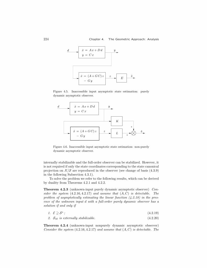
224 Chapter 4. The Geometric Approach: Analysis
z
x = Ax+Dd
y = C x
d y
Eex = (A+GC) z
− Gy
Figure 4.5. Inaccessible input asymptotic state estimation: purely
dynamic asymptotic observer.
+
+
z
x = Ax+Dd
y = C x
d y
K
ex = (A+GC) z
− GyL
Figure 4.6. Inaccessible input asymptotic state estimation: non-purely
dynamic asymptotic observer.
internally stabilizable and the full-order observer can be stabilized. However, itis not required if only the state coordinates corresponding to the state canonicalprojection on X/S are reproduced in the observer (see change of basis (4.3.9)in the following Subsection 4.3.1).
To solve the problem we refer to the following results, which can be derivedby duality from Theorems 4.2.1 and 4.2.2.
Theorem 4.2.3 (unknown-input purely dynamic asymptotic observer) Con-sider the system (4.2.16, 4.2.17) and assume that (A,C) is detectable. Theproblem of asymptotically estimating the linear function (4.2.18) in the pres-ence of the unknown input d with a full-order purely dynamic observer has asolution if and only if
1. E ⊇ S∗ ; (4.2.19)
2. SM is externally stabilizable. (4.2.20)
Theorem 4.2.4 (unknown-input nonpurely dynamic asymptotic observer)Consider the system (4.2.16, 4.2.17) and assume that (A,C) is detectable. The

4.3. Unknown-Input Reconstructability, Invertibility, and Functional Controllability225
problem of asymptotically estimating linear function (4.2.18) in the presenceof the unknown input d with a full-order nonpurely dynamic observer has asolution if and only if
1. E ⊇ S∗ ∩ C ; (4.2.21)
2. SM is externally stabilizable. (4.2.22)
In (4.2.19, 4.2.21) S∗ is the subspace defined by (4.1.24), whereas in(4.2.20, 4.2.22) SM is the subspace defined by (4.2.10), which is the maximal(A, C ∩E)-conditioned invariant self-hidden with respect to D provided (4.2.19)or (4.2.21) holds.
When E = {0}, i.e., when an estimate of the whole state is sought, (4.2.20)cannot hold (of course, the trivial case D= {0} is excluded), so a nonpurelydynamic observer must be used. This is possible if the conditions stated in thefollowing corollary, immediately deductable from Theorem 4.2.4, are satisfied.
Corollary 4.2.1 Consider the system (4.2.16, 4.2.17) and suppose that (A,C)is detectable. The problem of asymptotically estimating the whole state in thepresence of the unknown input d has a solution with a nonpurely dynamicobserver if and only if
1. S∗ ∩ C = {0} ; (4.2.23)
2. S∗ is externally stabilizable. (4.2.24)
Computational “recipes” for matrices G,K,L of the observers representedin Fig. 4.5 and 4.6 will be considered in the next chapter (Subsection 5.1.2).
4.3 Unknown-Input Reconstructability, Invert-ibility, and Functional Controllability
The problem of observing the state in the presence of inaccessible inputs bymeans of a suitable asymptotically stable dynamic system (the estimator ordynamic observer) has been considered in the previous section as a basicapplication of conditioned invariance. In this section the same problem willbe considered in a more extended way and it will be shown that to obtainthe maximal information on state in the presence of inaccessible inputs it isnecessary to use differentiators , so the most general observers are not includedin the class of dynamic systems. In other words, the mathematical problem ofobtaining final state from input and output functions when some of the inputsare unknown has solvability conditions more extended than the problem ofestimating the state through a dynamic observer.
The need to use differentiators, which are linear operators, but not belong-ing to the class of linear dynamic systems considered in the first two chaptersof this book and not susceptible to any ISO representation, is pointed out by asimple example. Consider a dynamic system consisting of n cascaded integra-tors, with input u to the first and output y from the last: it can be represented

226 Chapter 4. The Geometric Approach: Analysis
by a triple (A, b, c), but its state (which consists of the integrator outputs)can be determined only by means of n− 1 cascaded differentiators connectedto output y. The technique described in the previous section, which uses adynamic system, clearly cannot be applied in this case.
From a strictly mathematical viewpoint, unknown-input observability isintroduced as follows. It is well known that the response of the triple (A,B,C)is related to initial state x(0) and control function u(·) by
y(t) = C eAt x(0) + C
∫ t
0
eA(t−τ)B u(τ) dτ (4.3.1)
where the first term on the right is the free response and the second is theforced response. In order to simplify notation, refer to a fixed time interval[0, T ]. Hence
y|[0,T ] = γ(x(0), u|[0,T ]
)= γ1
(x(0)
)+ γ2
(u|[0,T ]
)(4.3.2)
We recall that (A,C) is observable or reconstructable (in the continuous-time case these properties are equivalent) if γ1 is invertible, i.e., kerγ1 = {0}.In this case it is possible to derive the initial or the final state from inputand output functions. The following definitions extend the reconstructabilityconcept to the case where the input function is unknown and introduce theconcept of system invertibility, which will be proved to be equivalent to it(Theorem 4.3.1).
Definition 4.3.1 The triple (A,B,C) is said to be unknown-state, unknown-input reconstructable or unknown-state, unknown-input invertible if γ is in-vertible, i.e., kerγ= {0}.
Definition 4.3.2 The triple (A,B,C) is said to be zero-state, unknown-inputreconstructable or zero-state, unknown-input invertible if γ2 is invertible, i.e.,kerγ2 = {0}.
When (A,C) is not observable or reconstructable, the initial or final statecan be determined modulo the subspace
ker γ1 = Q := maxJ (A, C) (4.3.3)
which is called the unobservability subspace or the unreconstructability sub-space. This means that the state canonical projection on X/Q can be deter-mined from the output function. Q is the locus of the free motions correspond-ing to the output function identically zero.
Unknown-input reconstructability in the cases of the above definitions isapproached in a similar way: by linearity, when reconstructability is not com-plete, only the canonical projection of the final state on X/Q1 or on X/Q2 canbe determined, where Q1 is called the unknown-state, unknown-input unrecon-structability subspace and Q2 the zero-state, unknown-input unreconstructabil-ity subspace. Clearly Q2⊆Q1. Geometric expressions for these subspaces areprovided in the following properties.
4.3. Unknown-Input Reconstructability, Invertibility, and Functional Controllability227
Property 4.3.1 Refer to the triple (A,B,C). The unknown-state, unknown-input unreconstructability subspace is
Q1 = V∗0 := maxV(A,B, C) (4.3.4)
Proof. The statement is an immediate consequence of Theorem 4.1.1. �
Property 4.3.2 Refer to the triple (A,B,C). The zero-state, unknown-inputunreconstructability subspace is
Q2 = RV∗0= V∗0 ∩ S∗0 with S∗0 := minS(A, C,B) (4.3.5)
Proof. The statement is an immediate consequence of Theorem 4.1.6. �
4.3.1 A General Unknown-Input Reconstructor
We shall here describe how to implement a general unknown-input state re-constructor. First, we show that the current state is derivable modulo Q1 bymeans of an algebraic system with differentiators connected only to the systemoutput. The starting point is the relation
y(t) = C x(t) (4.3.6)
which, to emphasize the iterative character of the procedure, is written as
q0(t) = Y0 x(t) (4.3.7)
where q0 := y is a known continuous function in [0, T ] and Y0 :=C is a knownconstant matrix. The state modulo kerY0 can be derived from (4.3.7). Differ-entiating (4.3.7) and using the system equation x(t)=Ax(t)+B u(t) yields
q0(t)− Y0B u(t) = Y0Ax(t)
Let P0 be a projection matrix along im(Y0B), so that im(Y0B)=kerP0 and
P0 q0(t) = P0 Y0 Ax(t) (4.3.8)
Equations (4.3.7, 4.3.8) can be written together as
q1(t) = Y1 x(t)
where q1 denotes a known linear function of the output and its first derivative,and
Y1 :=
[Y0
P0 Y0A
]
228 Chapter 4. The Geometric Approach: Analysis
Simple manipulations provide
kerY1 = kerY0 ∩ ker(P0 Y0 A)
= kerY0 ∩ A−1Y −10 kerP0
= kerY0 ∩ A−1Y −10 Y0 imB
= kerY0 ∩ A−1(kerY0 + imB)
Iterating k times the procedure yields
qk(t) = Yk x(t)
where qk denotes a known linear function of the output and its derivatives upto the k-th, and Yk a matrix such that
kerYk = kerYk−1 ∩ A−1(kerYk−1 + imB)
= kerY0 ∩ A−1(kerYk−1 + imB)
where the last equality can be derived with an argument similar to that usedin the proof of Algorithm 4.1.1. Sequence kerYk (k=0, 1, . . .) converges toV∗0 , since it coincides with the sequence provided by Algorithm 4.1.2 to derivemaxV(A,B, C).
Note that the length of the observation interval [0, T ] has not been con-sidered in the preceding argument: since the described technique is based ondifferentiators, it is only required to be nonzero: functions qk(·) are continu-ous, hence differentiable, because each of them is obtained by projecting theprevious one along its possible discontinuity directions. Furthermore, from theargument it follows that the maximum order of the involved derivatives is n− 1.
We shall now prove that a dynamic device exists which, connected to thesystem output and with initial state suitably set as a linear function of thesystem state (which is assumed to be known), provides tracking of the systemstate modulo S∗0 . This device is quite similar to the unknown-input asymptoticestimators considered in the previous section, but it is not necessarily stable.Consider the identity observer shown in Fig. 3.10 and choose matrix G suchthat (A+GC)S∗0 ⊆S∗0 . The observer equations, expressed in the new basiscorresponding to the similarity transformation T := [T1 T2], with imT1 =S∗0 ,are [
η1(t)η2(t)
]=
[A′11 A′12O A′22
] [η1(t)η2(t)
]+
[B′1O
]u(t) +
[G′1G′2
]y(t) (4.3.9)
In (4.3.9), η denotes the new state, related to z by z=Tη. Zero submatricesare due to S∗0 being an (A+GC)-invariant containing B.
Note that only the second matrix differential equation of (4.3.9) (thatcorresponding to η2(t) at the left), has to be reproduced in the observer, sinceη2 is not influenced by η1 or u. If the observer initial state is set according toη(0)=T−1x(0), through
z2(t) = T2 η2(t) (4.3.10)

4.3. Unknown-Input Reconstructability, Invertibility, and Functional Controllability229
z1
x = Ax+B u
y = C x
u y algebraicreconstructor
(with differentiators)
zdynamic trackingdevice
z = M z1 +N z2
(x(0))
z2
Figure 4.7. The general block diagram of an unknown-input state reconstructor.
a state estimate modulo S∗0 is derived.The estimator scheme shown in Fig. 4.7 is based on both of the preceding
techniques: the algebraic reconstructor with differentiators provides as outputz1 a state estimate modulo Q1 and works if neither the initial state nor theinput function is known, while the dynamic tracking device provides as z2 astate estimate modulo S∗0 , but requires the initial state to be known. A stateestimate modulo Q2 is obtained as a linear function of the outputs of bothdevices. Note that the enlarged knowledge of the state obtained by algebraicreconstructor with differentiators is not useful in the dynamic device since ifS∗0 is replaced by minS(A,V∗0 ,B), the intersection in equation (4.3.5) does notchange owing to Corollary 4.1.1. The following properties, concerning completeunknown-input reconstructability, are particular cases of previous Properties4.3.1 and 4.3.2.
Property 4.3.3 The triple (A,B,C) is unknown-state, unknown-input com-pletely reconstructable in any finite time interval [0, T ] if and only if
V∗0 := maxV(A,B, C) = {0} (4.3.11)
Note that, if the triple (A,B,C) is unknown-state, unknown-input com-pletely reconstructable, the pair (A,C) is observable because of the inclusionmaxJ (A, C)⊆maxV(A,B, C).
Property 4.3.4 The triple (A,B,C) is zero-state, unknown-input completelyreconstructable in any finite time interval [0, T ] if and only if
V∗0 ∩ B = {0} (4.3.12)
Proof. An alternative expression for Q2 =RV∗ defined in (4.3.5) isQ2 =minJ (A+BF,V∗ ∩B), with F any matrix such that (A+BF )V∗⊆V∗.Therefore Q2 = {0} if and only if (4.3.12) holds. �
The state reconstructor shown in Fig. 4.7 provides the maximal informationon the system state when the input function is unknown and the initial state

230 Chapter 4. The Geometric Approach: Analysis
known, by observing the output in any nonzero time interval [0, T ]. The samescheme can also be used to provide an asymptotic state estimate when theinitial state is unknown, provided S∗0 is externally stabilizable. Since in thiscase matrix A′22 in (4.3.9) can be made stable by a suitable choice of G, functionz2(t) in (4.3.10) asymptotically converges to a state estimate modulo S∗0 alsoif the initial state of the dynamic tracking device is not congruent with that ofthe system. Necessary and sufficient conditions for complete state asymptoticestimation by means of a device including differentiators are stated in thefollowing property.
Property 4.3.5 The triple (A,B,C) is unknown-state, unknown-input com-pletely asymptotically observable if and only if
1. V∗0 ∩ B = {0} ; (4.3.13)
2. S∗0 is externally stabilizable. (4.3.14)
Proof. Recall Corollary 4.2.1 and note that processing the output throughthe algebraic reconstructor with differentiators provides the state modulo V∗0instead of modulo C. Hence (4.3.13) follows from (4.2.21) and from the proofof Property 4.3.4. �
Point 2 of Property 4.3.5 can also be expressed in terms of invariant ze-ros. The external unassignable eigenvalues of S∗0 or the internal unassignableeigenvalues of V∗0 , which are equal to each other owing to Property 4.1.20, arecalled the invariant zeros of the triple (A,B,C) (see next section). Therefore, ageneral unknown-state, unknown-input asymptotic estimator exists if and onlyif V∗0 ∩B reduces to the origin and all invariant zeros of the system are stable.
4.3.2 System Invertibility and Functional Controllability
Refer to a triple (A,B,C). The term system invertibility denotes the possibilityof reconstructing the input from the output function. Although for the sakeof precision it is possible to define both the unknown-state, unknown-inputinvertibility and the zero-state, unknown-input invertibility (see Definitions4.3.1 and 4.3.2, the term invertibility “tout court” is referred to the latter, i.e.,to the invertibility of map γ2 in (4.3.2).
The term functional controllability denotes the possibility of imposing anysufficiently smooth output function by a suitable input function, starting atthe zero state. Here “sufficiently smooth” means piecewise differentiable atleast n times. It is often also called right invertibility, from the identityy(·)= γ2(u(·)) ◦ γ−12 (y(·)), while simple invertibility is also called left invert-ibility, from u(·)= γ−12 (y(·)) ◦ γ2(u(·)).
Theorem 4.3.1 The triple (A,B,C), with B having maximal rank, isunknown-state (zero-state) invertible if and only if it is unknown-state,unknown-input (zero-state, unknown-input) completely reconstructable.

4.3. Unknown-Input Reconstructability, Invertibility, and Functional Controllability231
Proof. If. From the system differential equation x(t)=Ax(t)+B u(t) itfollows that
u(t) = (BTB)−1 BT(x(t)−Ax(t)
)(4.3.15)
which provides u(t) almost everywhere in [0, T ] if from y|[0,T ] (and x(0)) it ispossible to derive x|[0,T ], hence x|[0,T ] almost everywhere.
Only if. Let the considered system be invertible, i.e., from the outputfunction y|[0,T ] it is possible to derive input u|[0,T ]. By subtracting the forcedresponse from the total response we derive the free response, i.e., the outputfunction of the free system
x(t) = Ax(t)
y(t) = C x(t)
whose current state x(t) can be determined by repeatedly differentiating theoutput function if the initial state is unknown (recall that in this case completereconstructability implies complete observability) or by an identity observer ifknown. �
From now on, the term “invertibility” will be strictly referred to zero-stateinvertibility. The following statement is immediately derived from Theorem4.3.1 and Property 4.3.4.
Property 4.3.6 (left invertibility of a triple) The triple (A,B,C) is invertible(left-invertible) if and only if (4.3.12) holds.
The device whose block diagram is represented in Fig. 4.7 can easily beextended so as to be a realization of the inverse system of the triple (A,B,C):connect a further differentiator stage on output z1 (the time derivative of z2can be directly computed as a linear function of z2 and y): a linear algebraicblock implementing (4.3.15) will provide input u.
Owing to Property 4.3.5 and related discussion, the inverse system isasymptotically stable if and only if all the invariant zeros of (A,B,C) are stable(or, equivalently, V∗0 is internally stabilizable or S∗0 is externally stabilizable).
We shall now consider the dual concept and prove a theorem that is dualto Property 4.3.6.
Theorem 4.3.2 (functional controllability of a triple) The triple (A,B,C) isfunctionally output controllable (or right-invertible) if and only if
S∗0 + C = X (4.3.16)
Proof. Consider the linear operator γ2 in (4.3.2), which is left invertible ifand only if (4.3.12) holds. Its adjoint operator
u|[0,T ] = γT2(u|[0,T ]
)

232 Chapter 4. The Geometric Approach: Analysis
is defined by
u(t) = BT
∫ t
0
eAT (t−τ)CT y(τ) dτ t ∈ [0, T ]
From
(γT2 )−1 ◦ γT2 = i
where i denotes the identity operator, by taking the adjoint of both membersit follows that
γ2 ◦ γ−12 = i
Hence γ2 admits a right inverse if and only if γT2 admits a left inverse, i.e., ifand only if
maxV(AT , imCT , kerBT ) ∩ imCT = {0}
from which (4.3.16) follows by orthogonal complementation. �
The functional controller is realizable in exactly the same way as the inversesystem, i.e., by a state reconstructor of the type shown in Fig. 4.3 completedwith a further differentiator stage and an algebraic part. Its dynamic part isasymptotically stable if and only if all the invariant zeros of (A,B,C) are stable(or, equivalently, S∗0 is externally stabilizable or V∗0 is internally stabilizable).However, since in this case the system is not necessarily invertible, inputfunction u(·) corresponding to the desired output function is not in generalunique. On the other hand, the difference between any two admissible inputfunctions corresponds to a zero-state motion on RV∗
0which does not affect the
output function, so that the functional controller can be realized to provideany one of the admissible input functions, for instance by setting to zero inputcomponents which, expressed in a suitable basis, correspond to forcing actionsbelonging to V∗0 ∩B.
4.4 Invariant Zeros and the Invariant ZeroStructure
Consider a triple (A,B,C). The concept of “zero,” which is a natural coun-terpart to the concept of “pole” in IO descriptions, is introduced in geometricapproach terms through the following definition.6
6 In the literature concerning the matrix polynomial approach, the transmission zerosare defined as the zeros of the Smith-Macmillan form of the transfer matrix, while thoseintroduced in Definition 4.4-1 are usually named invariant zeros. These definitions ofzeros are equivalent to each other if (A,B, C) is minimal (i.e., completely controllable andobservable). In this case transmission or invariant zeros have a precise physical meaning,i.e., they “block” transmission of certain frequencies from input to output. Definition 4.4-1 is implicit in an early work by Morse [33] and specifically investigated by Molinari [31].Extensive reviews on definitions and meanings of multivariable zeros are reported by Francisand Wonham [19], MacFarlane and Karcanias [25], and Schrader and Sain [36].
4.4. Invariant Zeros and the Invariant Zero Structure 233
Definition 4.4.1 (invariant zeros) The invariant zeros of the triple (A,B,C)are the internal unassignable eigenvalues of V∗0 :=maxV(A,B, C) or, equiva-lently by virtue of Property 4.1.20, the external unassignable eigenvalues ofS∗0 :=minS(A, C,B).
Note that a system whose state or forcing action is completely accessible,i.e., with B=X or C= {0}, has no invariant zeros. Invariant zeros are easilycomputable by using the specific geometric approach algorithms.
A more complete definition, which includes the previous one as a particu-lar case, refers to the internal unassignable eigenstructure of V∗0 or the externalunassignable eigenstructure of S∗0 . The eigenstructure of a linear transforma-tion is complete information on its real or complex Jordan form (eigenvalues,number and dimensions of the corresponding Jordan blocks, or orders of cor-responding elementary divisors). As for the unassignable eigenvalues, matrixA′22 in (4.1.34) is referred to for the eigenstructures here considered.
Definition 4.4.2 (invariant zero structure) The invariant zero struc-ture of the triple (A,B,C) is the internal unassignable eigenstructure ofV∗0 :=maxV(A,B, C) or, equivalently, the external unassignable eigenstructureof S∗0 :=minS(A, C,B).
A quite common physical justification of the word “zero” is related to theproperty to block frequencies. It is worth discussing this property by referringto a suitable extension of the frequency response.
4.4.1 The Generalized Frequency Response
Refer to the block diagram in Fig. 2.4, which represents the quadruple(A,B,C,D), cascaded to an exosystem, described by the equations
v(t) = W v(t) (4.4.1)
u(t) = L v(t) (4.4.2)
We temporarily assume that A is asymptotically stable, whileW , the exosystemmatrix, is assumed to have all the eigenvalues with the real parts zero orpositive. For instance, the exosystem output could be one of those representedin Fig. 2.5) or any linear combinations of unstable modes.
The exosystem output is
u(t) = L eWt v0 (4.4.3)
Our aim is to search for conditions that ensure that the state evolution of thesystem, when the possible transient condition is finished, can be expressed asa function of the sole exogenous modes or, in other words, conditions for theexistence of a matrix X such that
limt→∞
x(t) = X eWt v0

234 Chapter 4. The Geometric Approach: Analysis
for any exosystem initial state v0. Function
xs(t) := X eWt v0 (4.4.4)
where xs is the state in the steady condition, is necessarily a solution of theoverall system differential equation and can be defined also when the systemmatrix A is unstable. By substituting it in the system differential equationx(t)=Ax(t)+B u(t) and taking into account (4.4.3) we get
XW eWt v0 = AX eWt v0 +B LeWt v0
Since v0 is arbitrary and the matrix exponential nonsingular, it follows that
AX −XW = −B L (4.4.5)
Matrix X is called state generalized frequency response. In general it is afunction of matrices W,L of the exosystem.
Relation (4.4.5) is a Sylvester equation: if for a given W it admits nosolution, the system is said to present a resonance atW ; owing to Theorem [2.5-10] this can occur only if the system and exosystem have common eigenvalues.Let
x(t) = xt(t) + xs(t)
Component xt is the state in the transient condition; since both x(t) and xs(t)satisfy the system differential equation, by difference we obtain
xt(t) = Axt(t)
whencext(t) = eAt x0t = eAt (x0 − x0s) (4.4.6)
where, according to (4.4.4), x0s =X v0 is the particular value of the initialcondition that makes the transient motion vanish, i.e., such that the equalityx(t)= xs(t) holds identically in time, not only as t approaches infinity.
As far as the output is concerned, by substituting (4.4.3) and (4.4.4) in theoutput equation y(t)=C x(t)+Du(t) it follows that
ys(t) = (C X +DL) eWt v0 = Y eWt v0 (4.4.7)
whereY := C X +DL (4.4.8)
is called the output generalized frequency response, which is also a function ofmatrices W,L of the exosystem.
Particular, interesting cases are those of an exosystem with a single realeigenvalue ρ and of an exosystem with a pair of complex conjugate eigenvaluesσ± jω, i.e.
W := ρ W :=
[σ ω−ω σ
](4.4.9)

4.4. Invariant Zeros and the Invariant Zero Structure 235
or, to consider multiple eigenvalues, the corresponding real Jordan blocks oforder k. For instance, in the cases of a double real eigenvalue and a pair ofcomplex conjugate eigenvalues with multiplicity two, we assume respectively
W :=
[ρ 10 ρ
]W :=
⎡⎢⎣
σ ω−ω σ
I2
Oσ ω−ω σ
⎤⎥⎦ (4.4.10)
In these cases matrix L is p× k or p× 2k and produces the distribution onthe system inputs of the exogenous modes corresponding to the consideredeigenvalues or Jordan blocks.
Referring to the generalized frequency response, it is possible to introducethe concepts of blocking zero and blocking structure as follows.
Definition 4.4.3 (blocking zero and blocking structure) A blocking zero ofthe quadruple (A,B,C,D) is a value of ρ or σ± jω such that for W defined asin (4.4.9) there exists at least one input distribution matrix L corresponding toa state generalized frequency response X such that the pair (W,X) is observableand the output generalized frequency response is zero. A blocking structure isdefined by extending the above to the case of an arbitrary W in real Jordanform.
In other words, a blocking zero or a blocking structure is an exosystemmatrix W such that there exists at least one zero-output state trajectory thatis a function of all the corresponding modes. Hence, for such a W there existmatrices X,L with (W,X) observable such that
AX −XW = −BL (4.4.11)
C X +DL = O (4.4.12)
Equations (4.4.11, 4.4.12) are linear in X,L for any W . In the case of a purelydynamic system (i.e., for D=O) blocking zeros or blocking structures are notaffected by state feedback or output injection. In fact, X0,W0, and L0 satisfy(4.4.11, 4.4.12) with D=O. Then
(A+B F )X0 −X0W0 = −BL1 , with L1 := L0 − F X0
(A+GC)X0 −X0W0 = −BL0 , since C X0 = O
Invariant zeros and the invariant zero structure are related to blocking zerosand blocking structures, as the following properties state.
Property 4.4.1 Consider a triple (A,B,C). Its invariant zeros and the in-variant zero structure are also blocking zeros and a blocking structure.
Proof. Let F be such that (A+BF )V∗0 ⊆V∗0 : among all possible state feed-back matrices, this corresponds to the maximal unobservability subspace, sinceV∗0 is the maximal controlled invariant contained in C. Furthermore, it allows

236 Chapter 4. The Geometric Approach: Analysis
all the eigenvalues to be arbitrarily assigned, except the internal unassignableeigenvalues of V∗0 , so we can assume that no other eigenvalue of A+BF is equalto them. On this assumption RV∗
0as an (A+BF )-invariant is complementable
with respect to ({0},V∗0 ): this means that there exists a V such that
RV∗0⊕ V = V∗0
(A+B F )V ⊆ V
Consider the change of basis defined by transformation T := [T1 T2 T3], withimT1=RV∗
0, imT2=V . Thus
T−1(A+BF )T =
⎡⎣A′11 O A′13O A′22 A′23O O A′33
⎤⎦ (4.4.13)
clearly the invariant zeros are the eigenvalues of A′22 (the invariant zero struc-ture is the eigenstructure of A′22). The statement follows by assuming
W := A′22 X := T2 L := F T2 (4.4.14)
In fact, it will be shown that the above matrices are such that
i) (X,W ) is observable;
ii) C X = O ;
iii) AX −XW = −B L .
Property i is due to the rank of X being maximal and equal to the dimensionof W , relation ii follows from imX =V ⊆V∗0 , while iii is equivalent to
AT2 − T2A′22 = −BF T2
i.e.
(A+B F )T2 = T2A′22
which directly follows from (4.4.13). �
Property 4.4.2 Let the triple (A,B,C) be completely controllable and (left)invertible. Its blocking zeros and blocking structures are invariant zeros andparts of the invariant zero structure.
Proof. Let (W,X) be the Jordan block and the state frequency responsecorresponding to a blocking zero, so that
AX −XW = −BL (4.4.15)
C X = O (4.4.16)

4.4. Invariant Zeros and the Invariant Zero Structure 237
This means that the extended free system
˙x(t) = A x(t) with A :=
[A BLO W
]
admits solutions of the type
x(t) = X eWt v0 with imX ⊆ V∗0 ⊆ C
Let F be a state feedback matrix such that (A+BF )V∗0 ⊆V∗0 ; by adding BFXto both members of (4.4.15) it follows that
(A+BF )X −XW = −B L+B F X
The image of the matrix on the right must belong to V∗0 since those of bothmatrices on the left do. On the other hand, provided V∗0 ∩B= {0} owing tothe invertibility assumption, matrix on the right is zero. Hence
(A+BF )X −XW = O
and, consequentlyx(t) = e(A+BF )tX v0 = X eWt v0
The pair (W,X) is observable by assumption. Since the modes correspondingto both matrix exponentials in the preceding relations must be identical infunction x(t), there exists a Jordan block in A+BF internal to V∗0 (in thiscase nonassignable, like all the eigenvalues internal to V∗0 ), equal to W . �
Note that, while Definitions 4.4.1 and 4.4.2 (invariant zero and invariantzero structure) refer to a quadruple, Definition 4.4.3 refers to a triple. On theother hand, its extension to quadruples can be achieved by using an artifice,i.e., by cascading to the system a stage of integrators, which does not presenteither invariant or blocking zeros, so that the invariant zeros and the invariantzero structure of the quadruple can be assumed to be equal to those of theaugmented system. This topic will be reconsidered in the next section.
4.4.2 The Role of Zeros in Feedback Systems
The concept of zero is of paramount importance in connection with stabilizabil-ity of feedback systems. It is well known from the automatic control systemsanalysis, which is normally developed by using transfer functions, that the pres-ence of zeros in the right-half s plane, i.e., the nonminimum phase condition,generally causes serious stabilizability problems. The preceding multivariableextension of the concept of zero strictly developed in the framework of the ge-ometric approach is similarly connected with stabilizability in the presence offeedback and plays a basic role in synthesis problems.
To clarify this by means of an example, we shall show here that thestabilizability condition for the disturbance localization problem and its dual

238 Chapter 4. The Geometric Approach: Analysis
(see Section 4.2) is susceptible to a quite simple and elegant reformulation interms of invariant zeros.
Referring to the system (4.2.1, 4.2.2), denote by Z(u ; e) the set of allinvariant zeros between input u and output e, and by Z(u, d ; e) that betweeninputs u, d (considered as a whole), and output e. The basic result is set in thefollowing theorem.
Theorem 4.4.1 Let D⊆V∗ or D⊆V∗+B, with V∗ :=maxV(A,B, E). ThenVm :=V∗ ∩S∗1 , with S∗1 :=minS(A, E ,B+D), is internally stabilizable if andonly if all the elements of Z(u ; e) − Z(u, d ; e) are stable (recall that − denotesdifference with repetition count).
Proof. It has been proved in Section 4.2 that the assumption regarding Dimplies maxV(A,B, E)=maxV(A,B+D, E), so that the reachable set on E bythe only input u is RE :=V∗ ∩minS(A, E ,B), while the reachable set by bothinputs u, d used together is Vm :=V∗ ∩minS(A, E ,B+D).
Assume a coordinate transformation T := [T1 T2 T3 T4] with imT1=RE ,im[T1 T2] =Vm, im[T1 T2 T3] =V∗, im[T1 T4]⊇B, im[T1 T2 T4]⊇S∗1 ⊇D. Matri-ces A′ :=T−1AT , B′ :=T−1B and D′ :=T−1D have the structures
A′ =
⎡⎢⎣A′11 A′12 A′13 A′14O A′22 A′23 A′24O O A′33 A′34A′41 A′42 A′43 A′44
⎤⎥⎦ B′ =
⎡⎢⎣B′1OOB′4
⎤⎥⎦ D′ =
⎡⎢⎣D′1D′2OD′4
⎤⎥⎦
where the zero submatrices of A′ are due to RE and Vm being respectively an(A,B)- and an (A,B+D)-controlled invariant and to the structures of B′ andD′. The elements of Z(u ; e) are the union of the eigenvalues of A′22 and A′33,while those of Z(u, d ; e) are the eigenvalues of A′33. �
The main results of disturbance localization and unknown-input asymptoticstate estimation can be reformulated as follows.
Corollary 4.4.1 (inaccessible disturbance localization) Consider the system(4.2.1, 4.2.2) and assume that (A,B) is stabilizable. The inaccessible distur-bance localization problem with stability has a solution if and only if
1. D ⊆ V∗ ; (4.4.17)
2. Z(u ; e) − Z(u, d ; e) has all its elements stable. (4.4.18)
Corollary 4.4.2 (accessible disturbance localization) Consider the system(4.2.1, 4.2.2) and assume that (A,B) is stabilizable. The accessible disturbancelocalization problem with stability has a solution if and only if
1. D ⊆ V∗ + B ; (4.4.19)
2. Z(u ; e) − Z(u, d ; e) has all its elements stable. (4.4.20)

4.5. Extensions to Quadruples 239
The dual results are stated as follows. Consider the system (4.2.16–4.2.18)and denote by Z(d ; e) the set of all invariant zeros between input u and outpute and by Z(d ; y, e) that between input d and outputs y, e (considered as awhole).
Theorem 4.4.2 Let E ⊇S∗ or D⊇S∗ ∩C, with S∗ :=minS(A, C,D). ThenSM :=S∗+maxV(A,D, C ∩E) is externally stabilizable if and only if all theelements of Z(d ; y) − Z(d ; y, e) are stable.
Corollary 4.4.3 (unknown-input purely dynamic asymptotic observer) Con-sider the system (4.2.16, 4.2.17) and assume that (A,C) is detectable. Theproblem of asymptotically estimating the linear function e(t)=E x(t) in thepresence of the unknown input d with a full-order purely dynamic observer, hasa solution if and only if
1. E ⊇ S∗ ; (4.4.21)
2. Z(d ; y) − Z(d ; y, e) has all its elements stable. (4.4.22)
Corollary 4.4.4 (unknown-input nonpurely dynamic asymptotic observer)Consider the system (4.2.16, 4.2.17) and assume that (A,C) is detectable. Theproblem of asymptotically estimating the linear function e(t)=E x(t) in thepresence of the unknown input d with a full-order purely dynamic observer hasa solution if and only if
1. E ⊇ S∗ ∩ C ; (4.4.23)
2. Z(d ; y) − Z(d ; y, e) has all its elements stable. (4.4.24)
4.5 Extensions to Quadruples
Most of the previously considered problems were referred to purely dynamicsystems of the type (A,B,C) instead of nonpurely dynamic systems of thetype (A,B,C,D), which are more general. There are good reasons for this:triples are quite frequent in practice, referring to triples greatly simplifiesarguments, and extension to quadruples can often be achieved by using somesimple, standard artifices.
A very common artifice that can be adopted for many analysis problemsis to connect an integrator stage in cascade to the considered quadruple, atthe input or at the output: in this way an extended system is obtained thatis modeled by a triple. Problems in which smoothness of the input or out-put function is a standard assumption, like unknown-input reconstructability,invertibility, functional controllability, introduction of the concepts of trans-mission zero and zero structure, can thus be extended to quadruples withoutany loss of generality.
Consider the connections shown in Fig. 4.8: in the case of Fig. 4.8,a theoverall system is modeled by
˙x(t) = A x(t) + B v(t) (4.5.1)
y(t) = C x(t) (4.5.2)

240 Chapter 4. The Geometric Approach: Analysis
y
u = vv u x = Ax+B u
y = C x+Du
y
x = Ax+B u
y = C x+Duz = y
u z
(a)
(b)
Figure 4.8. Artifices to reduce a quadruple to a triple.
with
x :=
[xu
]A :=
[A BO O
]B :=
[OIp
]C := [C D ] (4.5.3)
while in the case of Fig. 4.8(b) the system is described by
˙x(t) = A x(t) + B u(t) (4.5.4)
z(t) = C x(t) (4.5.5)
with
x :=
[xz
]A :=
[A OC O
]B :=
[BD
]C := [O Iq ] (4.5.6)
To approach unknown-input reconstructability and system invertibility itis quite natural to refer to the extended system shown in Fig. 4.8(a), while forfunctional controllability, that of Fig. 4.8(b) is preferable. For invariant zerosand the invariant zero structure, any one of the extended systems can be used,since in both cases the integrator stage has no influence on zeros.
We shall now consider in greater detail the extension of the concept of zero,referring to (4.5.4–4.5.6). A controlled invariant contained in C := kerC can beexpressed as
V =
{[xz
]: x ∈ V , z = 0
}(4.5.7)
because of the particular structure of C. The definition property
AV ⊆ V + B (4.5.8)
implies
AV ⊆ V + B (4.5.9)
C V ⊆ imD (4.5.10)

4.5. Extensions to Quadruples 241
From (4.5.9) it follows that V is an (A,B)-controlled invariant. Since anymotion on the “extended” controlled invariant V satisfies z(·)= 0, then y(·)= 0,any state feedback matrix such that (A+ BF )V ⊆ V has the structure F = [F O]with
(A+B F )V ⊆ V V ⊆ ker (C +DF ) (4.5.11)
Relations (4.5.7, 4.5.8) and (4.5.11) can be considered respectively the defi-nition and main property of a geometric tool similar to the controlled invariant,which is called in the literature output-nulling controlled invariant .7
Of course, being an extension of the regular controlled invariant, it satisfiesall its properties, including the semilattice structure. A special algorithm toderive the maximal output-nulling controlled invariant is not needed, since itis possible to use the standard algorithm for the maximal controlled invariantreferring to the extended system (4.5.4–4.5.6).
The dual object, the input-containing conditioned invariant can also bedefined, referring to (4.5.1–4.5.3) instead of (4.5.4–4.5.6).
A conditioned invariant of the extended system containing B := imB canbe expressed as
S =
{[xu
]: x ∈ S , u ∈ R
p
}(4.5.12)
because of the particular structure of B. Relation
A (S ∩ C) ⊆ S (4.5.13)
together with (4.5.12) implies
A (S ∩C) ⊆ S (4.5.14)
B−1 S ⊇ kerD (4.5.15)
It follows that a conditioned invariant S is input-containing if and only if thereexists an extended output injection GT = [GT O] such that
(A+GC)S ⊆ S S ⊇ im (B +GD) (4.5.16)
The minimal input-containing conditioned invariant is the minimalzero-state unknown-input unreconstructability subspace of the quadruple(A,B,C,D) by means of a device of the type shown in Fig. 4.7.
The maximal output-nulling controlled invariant and the minimal input-containing conditioned invariant can be determined by means of the stan-dard algorithms referring respectively to the extended system (4.5.4–4.5.6)and (4.5.1–4.5.3). Denote them by V∗0 and S∗0 : it can easily be checkedthat the reachable set on V∗0 is V∗0 ∩S∗0 and the unobservable set contain-ing S∗0 is V∗0 +S∗0 . The invariant zeros of (A,B,C,D) are the elements ofσ((A+BF )|V∗
0 /(V∗0∩S∗
0 )) or those of σ((A+GC)|(V∗
0+S∗0 )/S∗
0): it is easy to show
that these two spectra are identical. The invariant zero structure of (A,B,C,D)coincides with any of the eigenstructures of the corresponding induced maps.
7 The output-nulling (controlled) invariants were introduced and investigated by Anderson[2,3]. Deep analysis of their properties, definition of their duals, and a complete bibliographyare due to Aling and Schumacher [1].

242 Chapter 4. The Geometric Approach: Analysis
+
_
u
x = Ax+B u
y = C x+Du
u
D
y
x = Ax+B u
y = C x+Du
y1
u = vv y
y1 ≡ u
(a)
(b)
Figure 4.9. Other artifices to deal with quadruples.
Feedback Connections. When a quadruple, which is a nonpurely dynamicsystem and hence has an algebraic signal path directly from input to output,is subject to nonpurely dynamic or simply algebraic feedback, like state feed-back and output injection, an algebraic closed loop is present and the stabilityproblem cannot be properly approached. In these cases, in general, the as-sumed mathematical model is not correct for the problem concerned and someneglected dynamics have to be considered.
Nevertheless, there exist artifices that allow standard feedback connectionsapproached for triples to be extended to quadruples. One of these is shownin Fig. 4.9(a): signal Du is subtracted from the output, thus obtaining a newoutput y1 which can be used for a possible feedback connection. In this way,for instance, the quadruple (A,B,C,D) can be stabilized through an observerexactly in the same way as the triple (A,B,C).
A drawback of this procedure is that the system feature of being purelydynamic is not robust with respect to uncertainty in D, so that it is oftenpreferable to use one of the artifices shown in Fig. 4.8 again, but providing themaximal observability in the first case and the maximal controllability in thesecond. For instance, in the first case this is obtained as shown in Fig. 4.9(b),i.e., by including also the auxiliary state variables, which are accessible, in theoutput distribution matrix C, which becomes
C :=
[C DO Ip
]
4.5.1 On Zero Assignment
In some multivariable synthesis problems it is necessary to assign invariant zerosthrough a convenient choice of the system matrices. Refer to a controllable pair(A,B) and consider the problem of deriving suitable matrices C,D such that

4.5. Extensions to Quadruples 243
the quadruple (A,B,C,D) has as many as possible zeros arbitrarily assigned,or, by duality, given the observable pair (A,C) derive B,D such that again(A,B,C,D) has as many as possible zeros arbitrarily assigned. These problemsare both reduced to standard pole assignment by state feedback. Denote byp and q respectively the number of the inputs and that of the outputs of thequadruple to be synthesized.
Algorithm 4.5.1 (zero assignment for a quadruple) Let (A,B) be controllableand p≤ q. It is possible to assign n invariant zeros of the quadruple (A,B,C,D)by the following procedure:
1. Choose D arbitrary of maximal rank;
2. Derive F such that A+BF has the zeros to be assigned as eigenvalues;
3. Assume C := −DF .
Proof. Refer to the extended system (4.5.6) and assume
V∗ := kerC =
[InO
](4.5.17)
Being p≤ q and D of maximal rank, clearly
V∗ ∩ B = {0} (4.5.18)
Due to the particular choice of C, F := [F O] is such that
A+ B F =
[A+BF O
O O
]
This means that V∗ is an (A + BF )-invariant (hence the maximal (A, B)-controlled invariant contained in kerC) and its internal eigenvalues are thoseof A+BF . Due to (4.5.18) all these eigenvalues are unassignable, hence theycoincide with the invariant zeros of (A,B,C,D). �
If p≥ q, the preceding algorithm can be used to derive B,D instead of C,D,provided that (A,C) is observable. In fact, the invariant zeros of (A,B,C,D)coincide with those of (AT , CT , BT , DT ).

244 Chapter 4. The Geometric Approach: Analysis
References
1. Aling, H., and Schumacher, J.M., “A nine-fold canonical decompositionfor linear systems,” Int. J. Control , vol. 39, no. 4, pp. 779–805, 1984.
2. Anderson, B.D.O., “Output nulling invariant and controllability subspaces,”Proceedings of the 6th IFAC World Congress, paper no. 43.6, August 1975.
3. — , “A note on transmission zeros of a transfer function matrix,” IEEE Trans.Autom. Contr., vol. AC-21, no. 3, pp. 589–591, 1976.
4. Basile, G., and Marro, G., “Controlled and conditioned invariant subspacesin linear system theory,” J. Optimiz. Th. Applic., vol. 3, no. 5, pp. 305–315, 1969.
5. — , “On the observability of linear time-invariant systems with unknown inputs,”J. of Optimiz. Th. Applic., vol. 3, no. 6, pp. 410–415, 1969.
6. — , “L’invarianza rispetto ai disturbi studiata nello spazio degli stati,” Rendicontidella LXX Riunione Annuale AEI , paper 1-4-01, Rimini, Italy, 1969.
7. — , “A new characterization of some properties of linear systems: unknown-inputobservability, invertibility and functional controllability,” Int. J. Control , vol. 17,no. 5, pp. 931–943, 1973.
8. — , “Self-bounded controlled invariant subspaces: a straightforward approachto constrained controllability,” J. Optimiz. Th. Applic., vol. 38, no. 1, pp. 71–81,1982.
9. — , “Self-bounded controlled invariants versus stabilizability,” J. Optimiz. Th.Applic., vol. 48, no. 2, pp. 245–263, 1986.
10. Basile, G., Hamano, F., and Marro, G., “Some new results on unknown-input observability,” Proceedings of the 8th IFAC Congress, paper no. 2.1, 1981.
11. Basile, G., Marro, G., and Piazzi, A., “A new solution to the dis-turbance localization problem with stability and its dual,” Proceedings of the’84 International AMSE Conference on Modelling and Simulation, vol. 1.2, pp.19–27, Athens, 1984.
12. Bhattacharyya, S.P., “On calculating maximal (A,B)-invariant subspaces,”IEEE Trans. Autom. Contr., vol. AC-20, pp. 264–265, 1975.
13. — , “Observers design for linear systems with unknown inputs,” IEEE Trans.on Aut. Contr., vol. AC-23, no. 3, pp. 483–484, 1978.
14. Davison,E.J., andWang, S.H., “Properties and calculation of transmissionzeros of linear multivariable systems,” Automatica, vol. 10, pp. 643–658, 1974.
15. — , “Remark on multiple transmission zeros” (correspondence item), Automa-tica, vol. 10, pp. 643–658, 1974.
16. Desoer, C.A., and Schulman, J.D., “Zeros and poles of matrix transferfunctions and their dynamical interpretation,” IEEE Trans. Circ. Syst., vol. CAS-21, no. 1, pp. 3–8, 1974.
17. Dorato, P., “On the inverse of linear dynamical systems,” IEEE Trans. SystemSc. Cybern., vol. SSC-5, no. 1, pp. 43–48, 1969.
18. Fabian, E., and Wonham, W.M., “Decoupling and disturbance rejection,”IEEE Trans. Autom. Contr., vol. AC-19, pp. 399–401, 1974.

References 245
19. Francis, B.A., andWonham,W.M., “The role of transmission zeros in linearmultivariable regulators,” Int. J. Control , vol. 22, no. 5, pp. 657–681, 1975.
20. Fuhrmann, P.A., andWillems, J.C., “A study of (A,B)-invariant subspacesvia polynomial models,” Int. J. Control , vol. 31, no. 3, pp. 467–494, 1980.
21. Hautus, M.L.J., “(A,B)-invariant and stabilizability subspaces, a frequencydomain description,” Automatica, no. 16, pp. 703–707, 1980.
22. Kouvaritakis, B., and MacFarlane, A.G.J., “Geometric approach toanalysis and synthesis of system zeros - Part 1. Square systems,” Int. J. Control ,vol. 23, no. 2, pp. 149–166, 1976.
23. — , “Geometric approach to analysis and synthesis of system zeros - Part 2.Non-square systems,” Int. J. Control , vol. 23, no. 2, pp. 167–181, 1976.
24. MacFarlane, A.G.J., “System matrices,” Proc. IEE , vol. 115, no. 5, pp.749–754, 1968.
25. MacFarlane, A.G.J., and Karcanias, N., “Poles and zeros of linearmultivariable systems: a survey of the algebraic, geometric and complex-variabletheory,” Int. J. Control , vol. 24, no. 1, pp. 33–74, 1976.
26. Marro, G., “Controlled and conditioned invariants in the synthesis of unknown-input observers and inverse systems,” Control and Cybernetics (Poland), vol. 2,no. 3/4, pp. 81–98, 1973.
27. — , Fondamenti di Teoria dei Sistemi , Patron, Bologna, Italy, 1975.
28. Meditch, J.S., and Hostetter, G.H., “Observers for systems with un-known and inaccessible inputs,” Int. J. Control , vol. 19, pp. 473–480, 1974.
29. Molinari, B.P., “Extended controllability and observability for linear sys-tems,” IEEE Trans. Autom. Contr., vol. AC-21, pp. 136–137, 1976.
30. — , “A strong controllability and observability in linear multivariable control,”IEEE Trans. Autom. Contr., vol. AC-21, pp. 761–763, 1976.
31. — , “Zeros of the system matrix,” IEEE Trans. Autom. Contr., vol. AC-21, pp.795–797, 1976.
32. Morse, A.S., “Output controllability and system synthesis,” SIAM J. Control ,vol. 9, pp. 143–148, 1971.
33. — , “Structural invariants of linear multivariable systems,” SIAM J. Control ,vol. 11, pp. 446–465, 1973.
34. Pugh, A.C., and Ratcliffe, P.A., “On the zeros and poles of a rationalmatrix,” Int. J. Control , vol. 30, no. 2, pp. 213–226, 1979.
35. Sain, M.K., and Massey, J.L., “Invertibility of linear time-invariant dynam-ical systems,” IEEE Trans. Autom. Contr., vol. AC-14, no. 2, pp. 141–149, 1969.
36. Schrader, C.B., and Sain, M.K., “Research on system zeros: a survey,”Int. J. Control , vol. 50, no. 4, pp. 1407–1433, 1989.
37. Schumacher, J.M., “(C,A)-invariant subspaces: some facts and uses,” VrijeUniversiteit, Amsterdam, Holland, Report no. 110, 1979.
38. — , “Complement on pole placement,” IEEE Trans. Autom. Contr., vol. AC-25,no. 2, pp. 281–282, 1980.
39. — , “On a conjecture of Basile and Marro,” J. Optimiz. Th. Applicat., vol. 41,no. 2, pp. 371–376, 1983.

246 Chapter 4. The Geometric Approach: Analysis
40. Silverman, L.M., “Inversion of multivariable linear systems,” IEEE Trans.Autom. Contr., vol. AC-14, no. 3, pp. 270–276, 1969.
41. Wen, J.T., “Time domain and frequency domain conditions for strict positiverealness,” IEEE Trans. Autom. Contr., vol. 33, no. 10, pp. 988–992, 1988.
42. Wonham, W.M., “Algebraic methods in linear multivariable control,” SystemStructure, ed. A. Morse, IEEE Cat. n. 71C61, New York, 1971.
43. — , Linear Multivariable Control: A Geometric Approach, Springer-Verlag, NewYork, 1974.
44. Wonham, W.M., and Morse, A.S., “Decoupling and pole assignment inlinear multivariable systems: a geometric approach,” SIAM J. Control , vol. 8,no. 1, pp. 1–18, 1970.
45. — , “Feedback invariants of linear multivariable systems,” Automatica, vol. 8,
pp. 93–100, 1972.

Chapter 5
The Geometric Approach:Synthesis
5.1 The Five-Map System
In this chapter the features of the most general feedback connection, the output-to-input feedback through a dynamic system (or, simply, the output dynamicfeedback) are investigated and discussed. Two particular problems are pre-sented as basic applications of output dynamic feedback, namely the distur-bance localization problem by means of a dynamic compensator and the reg-ulator problem, which is the most interesting and complete application of thegeometric approach.
For either problem, a five-map system (A,B,C,D,E) is needed, modeledby
x(t) = Ax(t) +B u(t) +Dd(t) (5.1.1)
y(t) = C x(t) (5.1.2)
e(t) = E x(t) (5.1.3)
It is called the controlled system and is connected as shown in Fig. 5.1 to acontroller (compensator or regulator) described by
z(t) = N z(t) +M y(t) +Rr(t) (5.1.4)
u(t) = L z(t) +K y(t) + S r(t) (5.1.5)
The compensator is a device that influences the structural features of thecontrolled system to which it is connected, while the regulator influences boththe system structural features and asymptotic behavior. Themanipulable inputu is separate from the nonmanipulable input d, and the informative output yis separate from the regulated output e. When d is completely inaccessiblefor measurement, it is also called disturbance. Therefore, two distinct inputdistribution matrices, B and D, and two distinct output distribution matrices,C and E, are considered. The compensator or regulator is a nonpurely dynamicsystem with an input y (which coincides with the informative output of the
247

248 Chapter 5. The Geometric Approach: Synthesis
y
r
x = Ax+B u+Dd
y = C x
e = E x
d e
u
x = N z +M y +Rr
u = Lz +K y + S r
Figure 5.1. Controlled system and controller.
controlled system), a reference input r, which provides information on thecontrol tasks and possibly includes a part of d (when the nonmanipulable inputis accessible for measurement). In the overall system there are two separatestate vectors, x∈X :=Rn, the controlled system state, and z ∈Z :=Rm, thecontroller state.
The overall system considered is very general and versatile: by settingequal to zero some of its matrices it can reproduce in practice all control situ-ations: with dynamic or algebraic output feedback, with dynamic or algebraicprecompensation (feedforward), or with mixed feedback and feedforward.
The overall system inputs d and r are assumed to be completely general,i.e., to belong to the class of piecewise continuous functions. In solving con-trol system synthesis problems such a generality may be superfluous and toorestrictive: it may be convenient, for instance, to assume that all these inputsor a part of them are generated by a linear time-invariant exosystem. Since insynthesis the exosystem features directly influence some of the obtained regu-lator features (for instance order and structure), it is convenient to embed theexosystem matrix in that of the controlled system. The controlled system statewill be partitioned as
x =
[x1x2
](5.1.6)
where x1 denotes the state of the plant and x2 that of the exosystem. MatricesA,B,C,D,E are accordingly partitioned as
A =
[A1 A3
O A2
]B =
[B1
O
]D =
[D1
O
]C = [C1 C2 ] E = [E1 E2 ]
(5.1.7)
Note that the exosystem cannot be influenced by either input, but directlyinfluences both outputs. The controlled system structure is shown in Fig. 5.2.The system is not completely controllable, since inputs act only on the plant,but it is assumed to be completely observable (or, at least, reconstructable)

5.1. The Five-Map System 249
u y
x2 = A2 x2
x1 = A1 x1 + A3 x2 +
B1 u+D1 d
y = C1 x1 + C2 x2
e = E1 x1 + E2 x2
x2
d e
Figure 5.2. Controlled system including an exosystem.
through the informative output. In fact the regulator must receive information,direct or indirect, on all the exogenous modes to counterbalance their effectson the regulated output.
Summing up, the following assumptions are introduced:
1. the pair (A1, B1) is stabilizable
2. yje pair (A,C) is detectable
Note that the plant is a well-defined geometric object, namely the A-invariantdefined by
P :={x : x2 = 0
}(5.1.8)
The overall system represented in Fig. 5.1 is purely dynamic with two inputs,d and r, and one output, e. In fact, by denoting with
x :=
[xz
](5.1.9)
the extended state (controlled system and regulator state), the overall systemequations can be written in compact form as
˙x(t) = A x(t) + D d(t) + R r(t) (5.1.10)
e(t) = E x(t) (5.1.11)
where
A :=
[A+BKC BLMC N
]D :=
[DO
]
R :=
[BSR
]E := [E O ]
(5.1.12)
Note that, while the quintuple (A,B,C,D,E) that defines the controlledsystem is given, the order m of the regulator and matrices K,L,M,N,R, S are

250 Chapter 5. The Geometric Approach: Synthesis
y
x = Ax+B u+Dd
y = C x
e = E x
d e
u
x = N z +M y
u = Lz +K y
Figure 5.3. Reference block diagram for the disturbance localization
problem by dynamic compensator, and the regulator problem.
a priori unknown: the object of synthesis is precisely to derive them. Thus,the overall system matrices A, R are also a priori unknown.
In some important synthesis problems, like the disturbance localization bydynamic compensator, and the regulator problem (which will both be statedin the next section), input r is not present, so that the reference block diagramsimplifies as in Fig. 5.3.
5.1.1 Some Properties of the Extended State Space
We shall now show that geometric properties referring to A-invariants in theextended state space reflect into properties of (A,B)-controlled and (A, C)-conditioned invariants, regarding the controlled system alone. This makes itpossible to state necessary and sufficient conditions for solvability of the mostimportant synthesis problems in terms of the given quintuple (A,B,C,D,E).
The following property, concerning algebraic output-to-input feedback, isuseful to derive the basic necessary structural condition for dynamic compen-sator and regulator design.1
Property 5.1.1 Refer to the triple (A,B,C). There exists a matrix K suchthat a given subspace V is an (A+BKC)-invariant if and only if V is both an(A,B)-controlled and an (A, C)-conditioned invariant.
Proof. Only if. This part of the proof is trivial because if there exists amatrix K such that (A+BKC)V ⊆V clearly there exist matrices F :=KCand G :=BK such that V is both an (A+BF )-invariant and an (A+GC)-invariant, hence an (A,B)-controlled and an (A, C)-conditioned invariant.
If. Consider a nonsingular matrix T := [T1 T2 T3 T4], with imT1=V ∩C,im [T1 T2] =V , im [T1 T3] = C, and set the following equation in K:
K C [T2 T4] = F [T2 T4] (5.1.13)
1 See Basile and Marro [4.6], Hamano and Furuta [18].

5.1. The Five-Map System 251
Assume that C has maximal rank (if not, it is possible to ignore some outputvariables to meet this requirement and insert corresponding zero columns in thederived matrix). On this assumption C [T2 T4] is clearly a nonsingular squarematrix, so that the equation (5.1.13) admits a solution K for all F . Since V isan (A, C)-conditioned invariant
(A+BK C) imT1 = A (V ∩ C) ⊆ VOn the other hand, with KCT2=FT2 owing to (5.1.13), it follows that
(A+BK C) imT2 = (A+B F ) imT2 ⊆ (A+B F )V ⊆ V �
++
+
+
y
x = Ax+B u+Dd
y = C x
e = E x
d e
u
K
M
x = v
w = z
v w
N
L
Figure 5.4. Artifice to transform a dynamic output-to-input feedback
into an algebraic one.
It is now convenient to introduce a new formulation of the problem, wherethe synthesis of a dynamic regulator is precisely reduced to the derivation ofan algebraic output feedback for a new extended system, still of order n+m.2
The overall system of Fig. 5.3 is equivalent to that shown in Fig. 5.4, wherethe extended system
˙x(t) = A0 x(t) + B0 u(t) + D d(t) (5.1.14)
y(t) = C0 x(t) (5.1.15)
e(t) = E x(t) (5.1.16)
2 This artifice is due to Willems and Commault [37].

252 Chapter 5. The Geometric Approach: Synthesis
with state, input, and output defined as
x :=
[xz
]u :=
[uv
]y :=
[yw
](5.1.17)
and matrices
A0 :=
[A OO O
]B0 :=
[B OO Im
]D :=
[DO
]
C0 :=
[C OO Im
]E := [E O ]
(5.1.18)
is subject to the algebraic output feedback
K :=
[K LM N
](5.1.19)
Note that in (5.1.18) D and E are defined as in (5.1.12).The equivalence between the block diagrams of Fig. 5.3 and 5.4 and Prop-
erty 5.1.1 immediately leads to the following statement.
Property 5.1.2 Any extended subspace W that is an A-invariant is both an(A0, B0)-controlled and an (A0, C0)-conditioned invariant.
Consider the following subspaces of X (the controlled system state space):
P (W) :=
{x :
[xz
]∈ W
}(5.1.20)
I(W) :=
{x :
[x0
]∈ W
}(5.1.21)
which are called, respectively, the projection of W on X and the intersectionof W with X . They are effective tools to deal with extended systems.
In the extended state space the controlled system and controller state spacesare respectively
X :=
{[xz
]: z = 0
}Z :=
{[xz
]: x = 0
}(5.1.22)
They are orthogonal to each other and satisfy the following, easily derivablerelations:
P (W) = I(W + Z) (5.1.23)
I(W) = P (W ∩ X ) (5.1.24)
I((W ∩ X )⊥
)= P
((W ∩ X )⊥
)= I(W)⊥ (5.1.25)
P((W + Z)⊥
)= I
((W + Z)⊥
)= P (W)⊥ (5.1.26)

5.1. The Five-Map System 253
Property 5.1.3 The projection of the orthogonal complement of any extendedsubspace is equal to the orthogonal complement of its intersection:
P (W⊥) = I(W)⊥ (5.1.27)
Proof. Equalities (5.1.23) and (5.1.25) lead to
P (W⊥) = I(W⊥ + Z) = I((W ∩ X )⊥
)= I(W)⊥ �
Consider now the following lemma, which will be used in the next sectionto prove the nonconstructive necessary and sufficient conditions.
Lemma 5.1.1 Subspace V is an internally and/or externally stabilizable(A0, B0)-controlled invariant if and only if P (V) is an internally and/or ex-ternally stabilizable (A,B)-controlled invariant.
Proof. Only if. This part of the proof is an immediate consequence ofDefinitions 4.1.5 and 4.1.6 (internal and external stabilizability of a controlledinvariant).
If. Let V :=P (V) : it is easily seen that V can be expressed as
V :=
{[xz
]: x ∈ V , z =W x+ η , η ∈ L
}(5.1.28)
whereW denotes a suitablem×nmatrix and L a suitable subspace of the regu-lator state space Z. From (5.1.28) it clearly follows that dimV =dimV +dimL.Assume a basis matrix V of V and, if necessary, reorder its columns in such away that in the partition
V =
[V1 V2V3 V4
]
V1 is a basis matrix of V . Since all columns of V2 are linear combinations ofthose of V1, by subtracting these linear combinations a new basis matrix of Vcan be obtained with the structure
V ′ =
[V1 OV3 V ′4
]
where V1 and V ′4 have maximal rank. Any x∈ V can be expressed as
x =
[V1 OV3 V ′4
] [α1
α2
]
with α1, α2 properly dimensioned arbitrary real vectors, i.e., as
x = V1 α1
z = V3 α1 + V ′4 α2
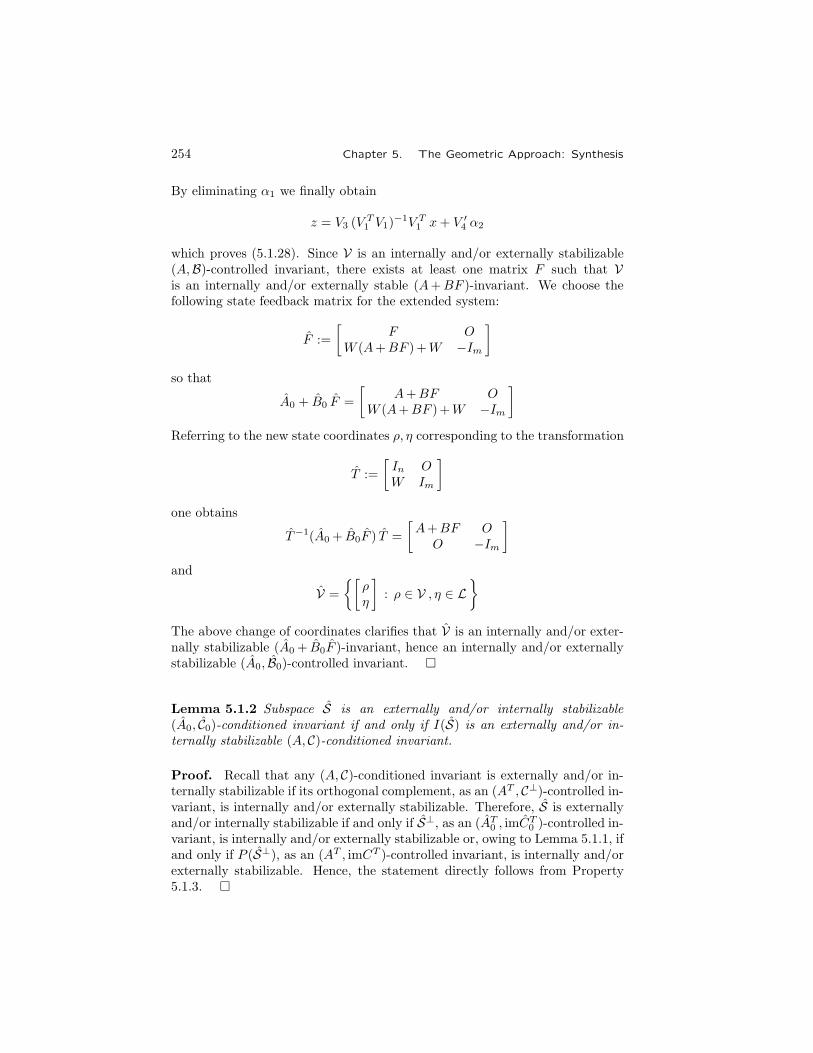
254 Chapter 5. The Geometric Approach: Synthesis
By eliminating α1 we finally obtain
z = V3 (VT1 V1)
−1V T1 x+ V ′4 α2
which proves (5.1.28). Since V is an internally and/or externally stabilizable(A,B)-controlled invariant, there exists at least one matrix F such that Vis an internally and/or externally stable (A+BF )-invariant. We choose thefollowing state feedback matrix for the extended system:
F :=
[F O
W (A+BF )+W −Im
]
so that
A0 + B0 F =
[A+BF O
W (A+BF )+W −Im
]
Referring to the new state coordinates ρ, η corresponding to the transformation
T :=
[In OW Im
]
one obtains
T−1(A0 + B0F ) T =
[A+BF O
O −Im
]
and
V =
{[ρη
]: ρ ∈ V , η ∈ L
}
The above change of coordinates clarifies that V is an internally and/or exter-nally stabilizable (A0 + B0F )-invariant, hence an internally and/or externallystabilizable (A0, B0)-controlled invariant. �
Lemma 5.1.2 Subspace S is an externally and/or internally stabilizable(A0, C0)-conditioned invariant if and only if I(S) is an externally and/or in-ternally stabilizable (A, C)-conditioned invariant.
Proof. Recall that any (A, C)-conditioned invariant is externally and/or in-ternally stabilizable if its orthogonal complement, as an (AT , C⊥)-controlled in-variant, is internally and/or externally stabilizable. Therefore, S is externallyand/or internally stabilizable if and only if S⊥, as an (AT
0 , imCT0 )-controlled in-
variant, is internally and/or externally stabilizable or, owing to Lemma 5.1.1, ifand only if P (S⊥), as an (AT , imCT )-controlled invariant, is internally and/orexternally stabilizable. Hence, the statement directly follows from Property5.1.3. �

5.1. The Five-Map System 255
5.1.2 Some Computational Aspects
The synthesis procedures that will be presented and used in the next sectioncan be considered extensions of dynamic systems stabilization by means ofobservers and dual observers, already discussed in Section 3.4.
In general, as a first step it is necessary to derive a matrix F suchthat a given internally and externally stabilizable controlled invariant V isan (A+BF )-invariant with A+BF stable or a matrix G such that a givenexternally and internally stabilizable conditioned invariant S is an (A+GC)-invariant with A+GC stable. The structure requirement can be imposed in-dependently of the stability requirement: for instance, as far as matrix F isconcerned, first derive an F1 such that (A+BF1)V ⊆V by means of Algorithm4.1-3, then express matrices A+BF1 and B in a basis whose vectors spanRV ,V ,X (which are (A+BF1)-invariants). Then apply an eigenvalue assign-ment procedure to the controllable pairs of submatrices (A′ij , B
′i) corresponding
to RV and X/V , which are respectively controllable by construction and sta-bilizable by assumption. In this way a matrix F2 is determined which, addedto F1, solves the problem. This procedure can be dualized for matrix G inconnection with conditioned invariants.
Refer to the block diagram of Fig. 3.11, where an identity observer isused to indirectly perform state feedback: the purely algebraic block F can beconsidered as connected between output z of the asymptotic observer shownin Fig. 3.12(b) and the system input u. Note that the same result is obtainedreferring to the dual observer of Fig. 3.12(c): a purely algebraic block G isconnected between a summing junction providing the difference η− y (of themodel and the system outputs) and the model forcing action ϕ.
In the former case, information on the system state to perform state feed-back is completely derived from the asymptotic observer, and the direct partialinformation provided by the system output is not taken into account. A moregeneral way to realize state feedback, which includes the complete direct statefeedback (which would be possible if C were square and nonsingular) and thecomplete indirect feedback through the observer as particular cases, is thatshown in Fig. 5.4(a). Information on state is there derived as a linear combi-nation of both the system output and the observer state (algebraic blocks L1
and L2 and summing junction), then applied to the system input through thealgebraic block F .
Let L1 and L2 satisfyL1C + L2 = In (5.1.29)
and apply to the extended system[x(t)z(t)
]=
[A+BFL1C BFL2
BFL1C −GC A+GC +BFL2
] [x(t)z(t)
]+
[DO
]d(t) (5.1.30)
the coordinate transformation expressed by[xz
]=
[In OIn −In
] [ρη
](5.1.31)

256 Chapter 5. The Geometric Approach: Synthesis
++
+
+
+
_
++
_
+_
+
y
y
x = Ax+B u+Dd
y = C x
e = E x
x = Ax+B u+Dd
y = C x
e = E x
d
d
e
e
u
u
G
G
z = Az + ϕ
z = Az + ϕ
C
C
η
η
ϕ
ϕ
L2
L2
L1
L1
B
B
F
F
z
(a)
(b)
Figure 5.5. Controllers based respectively on the identity observer and
the identity dual observer.
5.1. The Five-Map System 257
i.e., ρ :=x, η :=x− z. The equivalent system[ρ(t)η(t)
]=
[A+BF −BFL2
O A+GC
] [ρ(t)η(t)
]+
[DD
]d(t) (5.1.32)
is obtained. Note, in particular, that the separation property expressed byTheorem 3.4.6 still holds.
Fig. 5.5(b) shows the dual connection: difference η− y is processed throughthe algebraic block G, then applied both to the system input and the dualobserver forcing action through the algebraic blocks L1 and L2 and summingjunctions.
LetB L1 + L2 = In (5.1.33)
From the extended system, described by[x(t)z(t)
]=
[A+BL1GC BF −BL1GC−L2GC A+BF +L2GC
] [x(t)z(t)
]+
[DO
]d(t) (5.1.34)
through the coordinate transformation[xz
]=
[−In InO In
] [ρη
](5.1.35)
i.e., ρ :=x− z, η := z, the equivalent system[ρ(t)η(t)
]=
[A+GC OL2GC A+BF
] [ρ(t)η(t)
]+
[−DO
]d(t) (5.1.36)
is obtained. The separation property also clearly holds in this case.The crucial point of these procedures is the choice of matrices L1 and L2:
in fact, while respecting the constraints expressed by (5.1.29) and (5.1.33),it may be possible to impose further conditions that imply special structuralproperties for the overall system. The following lemmas provide a useful linkbetween geometric-type conditions and computational support for this problem.
Lemma 5.1.3 Let C be any q×n matrix and L a subspace of X such thatL∩C= {0}, with C := kerC. There exist two matrices L1, L2 such that
L1 C + L2 = In kerL2 = L (5.1.37)
Proof. Let Lc be any subspace that satisfies
L⊕ Lc = X Lc ⊇ C (5.1.38)
Define L2 as the projecting matrix on Lc along L, so that In−L2 is thecomplementary projecting matrix and ker (In−L2)=Lc. Hence, the equation
L1C = In − L2

258 Chapter 5. The Geometric Approach: Synthesis
is solvable in L1 owing to the second of (5.1.38). In fact, recall that thegeneric linear system AX =B or XTAT =BT is solvable in X if imA⊇ imBor kerAT ⊆ kerBT . �
Note that this proof is constructive, i.e., it provides a procedure to deriveL1, L2. The dual result, which is useful for synthesis based on the dual observer,is stated without proof as follows.
Lemma 5.1.4 Let B be any n× p matrix and L a subspace of X such thatL+B=X , with B := imB. There exist two matrices L1, L2 such that
B L1 + L2 = In imL2 = L (5.1.39)
Two Simple Applications. To show how the preceding lemmas can be usedin synthesis procedures, we shall look at two simple computational problems.First, consider again the unknown-input asymptotic observers whose blockdiagrams are shown in Fig. 4.5 and 4.6 or, in more compact form, in Fig. 5.6.
e
x = Ax+Dd
y = C x
e = E x
d
e
y
z = N z +M y
e = Lz +K y
Figure 5.6. Unknown-input nonpurely dynamic asymptotic observer.
Let S be our resolvent , i.e., an internally and externally stabilizable (A, C)-conditioned invariant such that S ⊇D and S ∩C ⊆E . First, determine a ma-trix G such that (A+GC)S ⊆S with A+GC stable. Assume N :=A+GC,M := −G, and K =O in the case of a purely dynamic observer. Our aim is toderive L in the purely dynamic case (it may be different from E if a reduced or-der device is sought) and K,L in the other case. To this end, derive a subspaceL that satisfies L⊕S ∩C = S (or L+S ∩C=S and L∩ (S ∩C)= {0}), i.e., acomplement of S ∩C to S. Clearly C ∩L= {0}. Owing to Lemma 5.1.3 thereexist two matrices L1, L2 such that L1C +L2= In, kerL2=L. Premultiplyingby E yields EL1C +EL2 =E, which, by assuming K :=EL1, L :=EL2, canalso be written as
K C + L = E with kerL ⊇ S (5.1.40)
To compute L1, L2, first derive a matrix X := [X1X2] such that imX1 =S ∩C,im[X1X2] =S, and assume L := imX2: clearly L∩C= {0}, L+S ∩C=S.
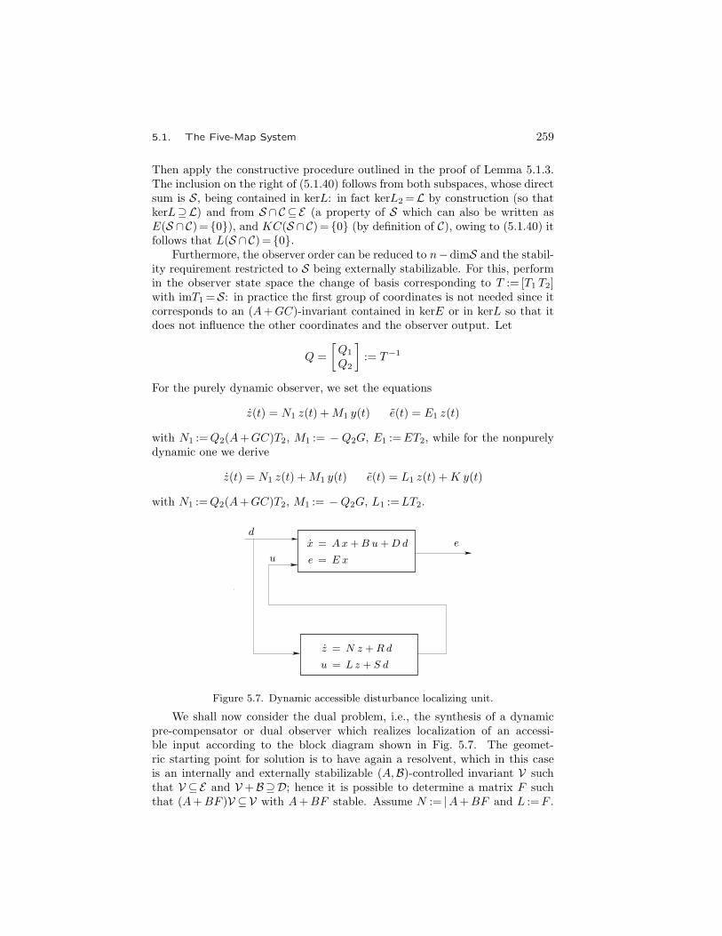
5.1. The Five-Map System 259
Then apply the constructive procedure outlined in the proof of Lemma 5.1.3.The inclusion on the right of (5.1.40) follows from both subspaces, whose directsum is S, being contained in kerL: in fact kerL2=L by construction (so thatkerL⊇L) and from S ∩ C ⊆E (a property of S which can also be written asE(S ∩C)= {0}), and KC(S ∩C)= {0} (by definition of C), owing to (5.1.40) itfollows that L(S ∩C)= {0}.
Furthermore, the observer order can be reduced to n−dimS and the stabil-ity requirement restricted to S being externally stabilizable. For this, performin the observer state space the change of basis corresponding to T := [T1 T2]with imT1 =S: in practice the first group of coordinates is not needed since itcorresponds to an (A+GC)-invariant contained in kerE or in kerL so that itdoes not influence the other coordinates and the observer output. Let
Q =
[Q1
Q2
]:= T−1
For the purely dynamic observer, we set the equations
z(t) = N1 z(t) +M1 y(t) e(t) = E1 z(t)
with N1 :=Q2(A+GC)T2, M1 := − Q2G, E1 :=ET2, while for the nonpurelydynamic one we derive
z(t) = N1 z(t) +M1 y(t) e(t) = L1 z(t) +K y(t)
with N1 :=Q2(A+GC)T2, M1 := −Q2G, L1 :=LT2.
x = Ax+B u+Dd
e = E x
de
u
z = N z +Rd
u = Lz + S d
Figure 5.7. Dynamic accessible disturbance localizing unit.
We shall now consider the dual problem, i.e., the synthesis of a dynamicpre-compensator or dual observer which realizes localization of an accessi-ble input according to the block diagram shown in Fig. 5.7. The geomet-ric starting point for solution is to have again a resolvent, which in this caseis an internally and externally stabilizable (A,B)-controlled invariant V suchthat V ⊆E and V +B⊇D; hence it is possible to determine a matrix F suchthat (A+BF )V ⊆V with A+BF stable. Assume N := |A+BF and L :=F .

260 Chapter 5. The Geometric Approach: Synthesis
Then, determine a subspace L that satisfies L∩V +B=V and L+(V +B)=X .Clearly B+L=X . Owing to Lemma 5.1.3 there exist two matrices L1, L2 suchthat BL1 +L2 = In, imL2 =L. Postmultiplying byD yields BL1D+L2D=Dwhich, by assuming S := − L1D, R :=L2D, can also be written as
−BS +R = D with imR ⊆ V (5.1.41)
The last condition follows from both subspaces whose intersection is S con-taining imR: in fact imL2=L by construction (so that imR⊆L) and fromV +B⊇D (a property of V which can also be written as D−1(V +B)=X ),and (BS)−1(V +B)=X (by definition of B), owing to (5.1.41) it follows thatR−1(V +B)=X or V +B⊇ imR.
Furthermore, the dual observer order can be reduced to dimV and thestability requirement restricted to V being internally stabilizable. For this,perform in the dual observer state space the change of basis corresponding toT := [T1 T2] with imT1=V : in practice the second group of coordinates is notneeded since all the zero-state admissible trajectories are restricted to the firstgroup, which is an (A+BF )-invariant containing imR so that it coincides withthe reachable subspace of the dual observer. The recipe for the localizing unitis stated as follows: let
Q =
[Q1
Q2
]:= T−1
and set the equations
z(t) = N1 z(t) +R1 d(t) y(t) = L1 z(t) + S d(t)
with N :=Q1(A+BF )T1, R1 :=Q1R, L1 :=FT1.
5.1.3 The Dual-Lattice Structures
Theorems 4.1.4 and 4.1.5 point out an interesting connection between con-trolled and conditioned invariants, which no longer appear as separate objects,connected only by duality relations, but as elements that are both necessary toderive remarkably simple and elegant algebraic expressions: see, for instance,expressions (4.1.30, 4.1.32), which provide the constrained reachable set and itsdual.
In this subsection the algebraic basic structures of lattices Φ(∗,∗) and Ψ(∗,∗),introduced in Section 4.1, are presented and investigated as a convenient back-ground to their use in solving synthesis problems. Structures will be graphicallyrepresented by means of Hasse diagrams referring to the inclusion, which al-low a simple representation of relations between the elements that contributeto problem solution, some a priori known and some available through suitablealgorithms.
First, we refer to the triple (A,B,C) and consider the fundamental latticesΦ(B,C) and Ψ(C,B), with B := imB, C := kerC. This particular case will be usedas a reference to derive more complex structures, like those that are used in

5.1. The Five-Map System 261
connection with quintuple (A,B,C,D,E) to solve synthesis problems. Thebasic property that sets a one-to-one correspondence between the lattice of all(A,B)-controlled invariants self-bounded with respect to C and that of (A, C)-conditioned invariants self-hidden with respect to B, is stated as follows.
Property 5.1.4 Let V be any (A,B)-controlled invariant contained in C, andS any (A, C)-conditioned invariant containing B: then
1. V ∩S is an (A,B)-controlled invariant;
2. V +S is an (A, C)-conditioned invariant.
Proof. From
A (S ∩ C) ⊆ S S ⊇ B (5.1.42)
AV ⊆ V + B V ⊆ C (5.1.43)
it follows that
A (V ∩S) = A (V ∩S ∩C) ⊆ AV ∩ A (S ∩C) ⊆ (V +B) ∩ S = V ∩S + B
A((V +S) ∩ C
)= A (V +S ∩C) = AV +A (S ∩ C) ⊆ V +B+S = V +S �
The fundamental lattices are defined as
Φ(B,C) :={V : AV ⊆ V + B , V ⊆ C , V ⊇ V∗0 ∩ B
}(5.1.44)
Ψ(C,B) :={S : A (S ∩ C) ⊆ S , S ⊇ B , S ⊆ S∗0 + C
}(5.1.45)
with
V∗0 := maxV(A,B, C) (5.1.46)
S∗0 := minS(A, C,B) (5.1.47)
Referring to these elements, we can state the following basic theorem.
Theorem 5.1.1 Relations
S = V + S∗0 (5.1.48)
V = S ∩ V∗0 (5.1.49)
state a one-to-one function and its inverse between Φ(B, C) and Ψ(C,B). Sumsand intersections are preserved in these functions.
Proof. V +S∗0 is an (A, C)-conditioned invariant owing to Property 5.1.4,self-hidden with respect to B since it is contained in S∗0 + C. Furthermore
(V + S∗0 ) ∩ V∗0 = V + S∗0 ∩ V∗0 = V

262 Chapter 5. The Geometric Approach: Synthesis
because V , being self-bounded with respect to C, contains the infimum ofΦ(B, C), V∗0 ∩S∗0 . By duality, S ∩V∗0 is an (A,B)-controlled invariant againby Property 5.1.4, self-bounded with respect to E because it contains V∗0 ∩B.Furthermore
(S ∩ V∗0 ) + S∗0 = S ∩ V∗0 + S∗0 = S
because S, being self-hidden with respect to B, is contained in the supremumof Ψ(B, C), V∗0 +S∗0 . Functions defined +by (5.1.48, 5.1.49) are one-to-onebecause, as just proved, their product is the identity in Φ(B,C) and their inverseproduct is the identity in Ψ(C,B). Since (5.1.48) preserves sums and (5.1.49)intersections and both are one-to-one, sums and intersections are preserved inboth functions. �
XX
C C+S∗0
V∗0
QB = QS∗0=
V∗0 + S∗
0
B ∩ V∗0 B
{0}{0}
free
free
fixed:Z (u; y)
fixed:Z (u; y)
Φ(B,C)S∗0
Ψ(C,B)
RC = RV∗0=
V∗0 ∩ S∗
0
S∗0
freeif (A, C) is
observable
freeif (A, C) is
controllable
∩V∗0
Figure 5.8. The fundamental lattices Φ(B,C) and Ψ(C,B).
Figure Fig. 5.8 shows the Hasse diagrams of the subspace sets that arereferred to in the definitions of the fundamental lattices. Thicker lines denotethe parts of the diagrams corresponding to lattices. Note that the eigenvalueassignability is also pointed out and the “zones” corresponding to invariantzeros of the triple (A,B,C) are specified in both lattices.
We shall now show that the above one-to-one correspondence can be ex-tended to other lattices, which are more directly connected with the searchfor resolvents for synthesis problems, which usually concerns the quintuple(A,B,C,D,E). Let D := imD, E := kerE, and assume
D ⊆ V∗ (5.1.50)

5.1. The Five-Map System 263
E E +S∗2 =
E + S∗i
V∗ +S∗1 =
V∗ + S∗2
V∗
Vm := V∗ ∩ S∗1
S∗2
{0} {0}
Ψ(E,B+D)
Z(u, d; e)+S∗2
RE = RV∗ =V∗ ∩ S∗
2
S∗1
Φ(B,E)Z(u; e)
Φ(B+D,E)Z(u, d; e)
Ψ(E,B)
Z(u; e)∩V∗
Figure 5.9. Lattices Φ(B,E) and Φ(B+D,E) (on the left) and their auxiliary duals.
By Property 4.2.1, on this assumption
V∗ :=maxV(A,B, E)=maxV(A,B+D, E) (5.1.51)
Consider the latticesΦ(B,E) and Φ(B+D,E) (5.1.52)
which, the latter being a part of the former (see Property 4.4.2), can berepresented in the same Hasse diagram, as shown in Fig. 5.9 In the figurethe following notations have been introduced:
S∗1 := minS(A, E ,B+D) (5.1.53)
S∗2 := minS(A, E ,B) (5.1.54)
Their auxiliary dual lattices are
Ψ(E,B) and Ψ(E,B+D) (5.1.55)
i.e., the lattices of all (A, E)-conditioned invariants self-hidden with respectto B and B+D, which can also be represented in the same Hasse diagram.Note that the elements of the second auxiliary lattice can be obtained bysumming S∗2 instead of S∗1 to the corresponding controlled invariants, sinceall these controlled invariants contain D. The dual-lattice diagram representedin Fig. 5.9 is obtained from the fundamental one simply by replacing B with

264 Chapter 5. The Geometric Approach: Synthesis
XX
QD = QS∗ =S∗ + V∗
2
V∗2
V∗1
S∗
DD ∩ V∗2 =
D ∩ V∗1
Ψ(C,D)
Z(d; y)+S∗
S∗ ∩ V∗2 =
S∗ ∩ V∗1
SM := S∗ +V∗1
Φ(D,C∩E)Z(d; y, e)
Φ(D,C)Z(d; y)
Ψ(C∩E,D)
Z(d; y, e)∩V∗
2
Figure 5.10. Lattices Ψ(C,D) and Ψ(C∩E,D) (on the right) and their auxiliary duals.
B+D and C with E . Also note that invariant zeros are related to lattices,being the unassignable internal or external eigenvalues of suitable well-definedsublattices of controlled or conditioned invariants.
All of the preceding is dualized as follows. Let
S∗ ⊇ E (5.1.56)
By the dual of Property 4.2.1, on this assumption
S∗ :=minS(A, C,D)=minS(A, C ∩E ,D) (5.1.57)
Consider the latticesΨ(C,D) and Ψ(C∩E,D) (5.1.58)
which, the latter being a part of the former (see Property 4.4.2), can berepresented in the same Hasse diagram, as shown in Fig. 5.10. In the figure,the following notations have been introduced:
V∗1 := maxV(A,D, C ∩E) (5.1.59)
V∗2 := maxV(A,D, C) (5.1.60)
Their auxiliary dual lattices are
Φ(D,C) and Φ(D,C∩E) (5.1.61)
5.1. The Five-Map System 265
i.e., the lattices of all (A,D)-controlled invariants self-bounded with respect toC and C ∩ E , which can also be represented in the same Hasse diagram.
The search for resolvents in connection with the most important synthesisproblems concerns the elements of lattices Φ(B+D,E) and Ψ(C∩E,D) (the lattice onthe left in Fig. 5.9 and that on the right in Fig. 5.10): in fact, resolvents are, ingeneral, an (A,B)-controlled invariant and an (A, C)-conditioned invariant bothcontained in E and containing D. It will be proved that restricting the choiceof resolvents to self-bounded controlled and self-hidden conditioned invariantsdoes not prejudice generality. A question now arises: is it possible to set a one-to-one correspondence directly between these lattices, so that stabilizabilityfeatures can be comparatively considered? The answer is affirmative: it canbe induced by a one-to-one correspondence between subsets of the auxiliarylattices, which are themselves lattices.
The elements of auxiliary lattices Φ(D,C∩E) and Ψ(E,B+D) are respectively(A,D)-controlled invariants contained in C ∩ E and (A, E)-conditioned invari-ants containing B+D. On the other hand, note that
AV ⊆ V +D ⇒ AV ⊆ V + B +D (5.1.62)
A (S ∩ E) ⊆ S ⇒ A (S ∩ C ∩ E) ⊆ S (5.1.63)
i.e., any (A,D)-controlled invariant is also an (A,B+D)-controlled invariantand any (A, E)-conditioned invariant is also an (A, C ∩E)-conditioned invari-ant. Unfortunately, not all the elements of Φ(D, C ∩E) are self-bounded withrespect to C ∩ E as (A,B+D)-controlled invariants, and not all the elementsof Ψ(E ,B+D) are self-hidden with respect to B+D as (A, C ∩E)-conditionedinvariants; the elements that meet this requirement belong to the sublattices
sub(Φ(B+D,C∩E)) :={V : V ∈ Φ(D,C∩E) , V ⊇ V∗1 ∩ (B+D)
}(5.1.64)
sub(Ψ(C∩E,B+D)) :={S : S ∈ Ψ(E,B+D) , S ⊆ S∗1 + (C ∩E)
}(5.1.65)
to which Theorem 5.1.1 can still be applied. Owing to Theorems 4.1.4 and4.1.5, the previous lattices can also be defined by the relations
sub(Φ(B+D,C∩E)) :={V : V ∈ Φ(D,C∩E) , V ⊇ V∗1 ∩ S∗1
}(5.1.66)
sub(Ψ(C∩E,B+D)) :={S : S ∈ Ψ(E,B+D) , S ⊆ V∗1 + S∗1
}(5.1.67)
which point out the new infimum and supremum, which are different from thoseof Φ(D,C∩E) and Ψ(E,B+D).
The sublattices of Φ(B+D,E) and Ψ(C∩E,D) defined by the one-to-onecorrespondences shown in Fig. 5.9 and 5.10 with the auxiliary sublattices(5.1.67, 5.1.66) are defined by
ΦR :={V : V ∈ Φ(B+D,E) , Vm ⊆ V ⊆ VM
}(5.1.68)
ΨR :={S : S ∈ Ψ(C ∩ E ,D) , Sm ⊆ S ⊆ SM
}(5.1.69)
with
Vm := V∗ ∩ S∗1 (5.1.70)
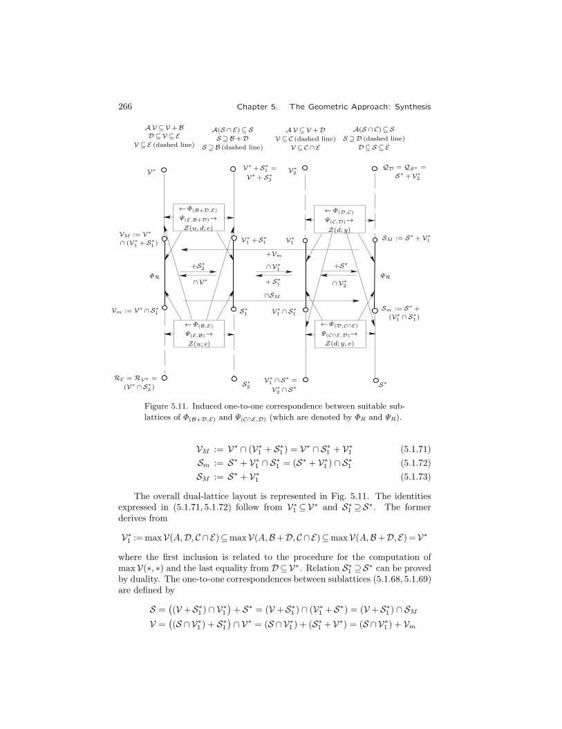
266 Chapter 5. The Geometric Approach: Synthesis
AV ⊆V +BD⊆V ⊆E
V ⊆E (dashed line)
A(S ∩E)⊆SS ⊇B+D
S ⊇B (dashed line)
AV ⊆V +DV ⊆C (dashed line)
V ⊆C ∩E
A(S ∩C)⊆SS ⊇D (dashed line)
D⊆S ⊆E
V∗ V∗ +S∗1 =
V∗ +S∗2
V∗2
QD = QS∗ =
S∗ +V∗2
VM := V∗
∩ (V∗1 +S∗
1 )
←Φ(D,C)
Ψ(C,D)→Z(d; y)
V∗1V∗
1 +S∗1
SM := S∗ +V∗1
ΦR
+S∗2
←Φ(B,E)
Ψ(E,B)→Z(u; e)
←Φ(B+D,E)
Ψ(E,B+D)→Z(u, d; e)
←Φ(D,C∩E)
Ψ(C∩E,D)→Z(d; y, e)
∩V∗1
+S∗1 ∩V∗
2
+S∗
∩V∗ ΨR
Vm := V∗ ∩S∗1 S∗
1 V∗1 ∩S∗
1Sm := S∗ +
(V∗1 ∩S∗
1 )
RE = RV∗ =
(V∗ ∩S∗2 )
S∗2
V∗1 ∩S
∗ =
V∗2 ∩S∗ S∗
+Vm
∩SM
Figure 5.11. Induced one-to-one correspondence between suitable sub-
lattices of Φ(B+D,E) and Ψ(C∩E,D) (which are denoted by ΦR and ΨR).
VM := V∗ ∩ (V∗1 + S∗1 ) = V∗ ∩ S∗1 + V∗1 (5.1.71)
Sm := S∗ + V∗1 ∩ S∗1 = (S∗ + V∗1 ) ∩ S∗1 (5.1.72)
SM := S∗ + V∗1 (5.1.73)
The overall dual-lattice layout is represented in Fig. 5.11. The identitiesexpressed in (5.1.71, 5.1.72) follow from V∗1 ⊆V∗ and S∗1 ⊇S∗. The formerderives from
V∗1 :=maxV(A,D, C ∩E)⊆maxV(A,B+D, C ∩E)⊆maxV(A,B+D, E)=V∗
where the first inclusion is related to the procedure for the computation ofmaxV(∗, ∗) and the last equality from D⊆V∗. Relation S∗1 ⊇S∗ can be provedby duality. The one-to-one correspondences between sublattices (5.1.68, 5.1.69)are defined by
S =((V +S∗1 ) ∩ V∗1
)+ S∗ = (V +S∗1 ) ∩ (V∗1 +S∗) = (V +S∗1 ) ∩ SM
V =((S ∩V∗1 ) + S∗1
)∩ V∗ = (S ∩V∗1 ) + (S∗1 +V∗) = (S ∩V∗1 ) + Vm

5.2. The Dynamic Disturbance Localization and the Regulator Problem 267
Note, in particular, that Vm and VM are (A,B)-controlled invariants self-bounded with respect to E , and that Sm and SM are (A, C)-conditioned invari-ants self-hidden with respect to D. These particular elements of Φ(B,E) andΨ(C,D) are very useful in the regulator and compensator synthesis procedures,which will be approached and thoroughly investigated in the next section.
5.2 The Dynamic Disturbance Localization and
the Regulator Problem
The solution of two basic problems, where the power of the geometric ap-proach is particularly stressed, will now be discussed. They are the disturbancelocalization by dynamic compensator and the regulator problem. First, noncon-structive but very simple and intuitive necessary and sufficient conditions, willbe derived. Then constructive necessary and sufficient conditions that directlyprovide resolvents - and so can be directly used for synthesis - will be statedfor the solvability of both problems.
For the disturbance localization by dynamic compensator we refer to theblock diagram of Fig. 5.3 and assume that the controlled system consists onlyof the plant, without any exosystem; thus it is completely stabilizable anddetectable.
Problem 5.2.1 (disturbance localization by dynamic compensator) Refer tothe block diagram of Fig. 5.3 and assume that (A,B) is stabilizable and (A,C)detectable. Determine, if possible, a feedback compensator of the type shown inthe figure such that:
1. e(t)= 0, t≥ 0, for all admissible d(·) and for x(0)= 0, z(0)=0 ;
2. lim t→∞ x(t)= 0 , lim t→∞ z(t)= 0 for all x(0), z(0) and for d(·)= 0 .
Condition 1 is the structure requirement and 2 the stability requirement .Problem 5.2.1 can be stated also in geometric terms referring to the extendedsystem (5.1.9–5.1.12), obviously with R=O.
Problem 5.2.2 (geometric formulation of Problem 5.2.1) Refer to the blockdiagram of Fig. 5.3 and assume that (A,B) is stabilizable and (A,C) detectable.Determine, if possible, a feedback dynamic compensator of the type shown inthe figure such that:
1. the overall system has an A-invariant W that satisfies
D ⊆ W ⊆ E with D := imD , E := kerE ;
2. A is stable.
Necessary and sufficient conditions for the solvability of Problem 5.2.1 aregiven in the following theorem in geometric terms regarding (A,B,C,D,E).3
3 This theorem is due to Willems and Commault [37].

268 Chapter 5. The Geometric Approach: Synthesis
Theorem 5.2.1 The disturbance localization problem by a dynamic compen-sator admits a solution if and only if there exist both an (A,B)-controlled in-variant V and an (A, C)-conditioned invariant S such that:
1. D ⊆ S ⊆ V ⊆ E ; (5.2.1)
2. S is externally stabilizable; (5.2.2)
3. V is internally stabilizable; (5.2.3)
Conditions stated in Theorem 5.2.1 are nonconstructive, since they refer toa resolvent pair (S,V) which is not defined. Equivalent constructive conditionsare stated as follows. They are formulated in terms of subspaces S∗,V∗,SM ,and VM defined in (5.1.57, 5.1.51, 5.1.73, 5.1.71).4
Theorem 5.2.2 The disturbance localization problem by a dynamic compen-sator admits a solution if and only if:
1. S∗ ⊆ V∗ ; (5.2.4)
2. SM is externally stabilizable; (5.2.5)
3. VM is internally stabilizable. (5.2.6)
We shall now consider the regulator problem. The formulation hereinpresented is very general and includes all feedback connections examined sofar as particular cases (disturbance localization, unknown-input asymptoticestimation, the above dynamic compensator). Moreover, it will be used as areference for further developments of the theory, like approach to reduced-orderdevices and robust regulation. We still refer to the block diagram of Fig. 5.3,assuming in this case that an exosystem is included as part of the controlledsystem, as in Fig. 5.2.5
Problem 5.2.3 (the regulator problem) Refer to the block diagram ofFig. 5.3, where the controlled system is assumed to have the structure of Fig. 5.2with (A11, B1) stabilizable and (A,C) detectable. Determine, if possible, a feed-back regulator of the type shown in Fig. 5.3 such that:
1. e(t)= 0, t≥ 0, for all admissible d(·) and for x1(0)=0, x2(0)=0, z(0)=0 ;
2. lim t→∞ e(t)= 0 for all x1(0), x2(0), z(0) and for d(·)= 0 ;
4 These constructive conditions without eigenspaces have been introduced by Basile,Marro, and Piazzi [6].
5 The regulator problem has been the object of very intensive research. The mostimportant contributions to its solution in the framework of the geometric approach are dueto Wonham [39] (problem without the stability requirement), Wonham and Pearson [40], andFrancis [17] (problem with the stability requirement). The statement reported here, whichincludes disturbance localization as a particular case, is due to Schumacher [31]. Theorem5.2.3, where the plant is explicitly introduced as a geometric object, is due to Basile, Marro,and Piazzi [8], as well as Theorem 5.2.4, where the stability requirement is handled withoutany use of eigenspaces [9].

5.2. The Dynamic Disturbance Localization and the Regulator Problem 269
3. lim t→∞ x1(t)= 0 , lim t→∞ z(t)= 0 for all x1(0), z(0) and for x2(0)=0,d(·)= 0 .
Condition 1 is the structure requirement , 2 the regulation requirement , and3 the stability requirement . Problem 5.2.3 can also be stated in geometricterms: first, define the extended plant as the A-invariant
P :=
⎧⎨⎩
⎡⎣x1x2z
⎤⎦ : x2 = 0
⎫⎬⎭ (5.2.7)
and refer again to the extended system (5.1.9–5.1.12) with R=O. The threepoints in the statement of Problem 5.2.3 can be reformulated as follows:
1. There exists an A-invariant W1 such that D ⊆ W1⊆ E ;2. There exists an externally stable A-invariant W2 such that W2⊆ E ;3. P , as an A-invariant, is internally stable.
Note that W := W1 + W2 is an externally stable A-invariant as the sum oftwo A-invariants, one of which is externally stable, so that P is internally stableif and only if W ∩ P is so. In fact, if P is internally stable, the invariant W ∩ P isalso internally stable, being contained in P. To prove the converse, consider thesimilarity transformation T := [T1 T2 T3 T4] with imT1 = W ∩ P , im [T1 T2] = P ,im [T1 T3] = W , which leads to
T−1A T =
⎡⎢⎣A′11 A′12 A′13 A′14O A′22 O A′24O O A′33 A′34O O O A′44
⎤⎥⎦
Submatrix A′11 is stable since W ∩P is internally stable, A′22 and A′44 are stablesince W is externally stable, so that P is internally stable as a consequence ofA′11 and A′22 being stable. Now Problem 5.2.3 can be stated in geometric termsas follows.
Problem 5.2.4 (geometric formulation of Problem 5.2.3Refer to the block diagram of Fig. 5.3, where the controlled system is
assumed to have the structure of Fig. 5.2 with (A1, B1) stabilizable and (A,C)detectable. Determine, if possible, a feedback regulator of the type shown inFig. 5.3 such that:
1. the overall system has an A-invariant W that satisfies
D ⊆ W ⊆ E , with D := imD , E := kerE ;
2. W is externally stable;
3. W ∩ P (which is an A-invariant) is internally stable.

270 Chapter 5. The Geometric Approach: Synthesis
Necessary and sufficient conditions for solvability of the regulator problemare stated in the following theorem, which can be considered as an extensionof Theorem 5.2.1.
Theorem 5.2.3 The regulator problem admits a solution if and only if thereexist both an (A,B)-controlled invariant V and an (A, C)-conditioned invariantS such that:6
1. D ⊆ S ⊆ V ⊆ E ; (5.2.8)
2. S is externally stabilizable; (5.2.9)
3. V is externally stabilizable; (5.2.10)
3. V ∩P is internally stabilizable. (5.2.11)
The corresponding constructive conditions are stated in the following the-orem, which extends Theorem 5.2.2.
Theorem 5.2.4 Let all the exogenous modes be unstable. The regulator prob-lem admits a solution if and only if:
1. S∗ ⊆ V∗ ; (5.2.12)
2. V∗ is externally stabilizable; (5.2.13)
3. SM is externally stabilizable; (5.2.14)
4. VM ∩P is internally stabilizable; (5.2.15)
5. VM +V∗ ∩P is complementable with respect to (VM ,V∗) . (5.2.16)
On stabilizability and complementability of controlled invariants, see Sub-section 4.1.4. The assumption that all the exogenous modes are unstable inpractice does not affect generality. In fact, any possible asymptotically stableexogenous mode can be eliminated in the mathematical model as it does notinfluence the asymptotic behavior of the overall system, since the extendedplant is required to be asymptotically stable.
5.2.1 Proof of the Nonconstructive Conditions
This subsection reports the proofs of Theorems 5.2.1 and 5.2.3. Of course, theyare related to each other, since the second theorem extends the first.
Proof of Theorem 5.2.1. Only if. Assume that conditions 1 and 2 stated inProblem 5.2.2 are satisfied. Hence, W is an A-invariant, so that, by virtue ofProperty 5.1.1, it is also an (A0, B0)-controlled and an (A0, C0)-conditioned in-variant, both internally and externally stabilizable since W is both an internallyand externally stable A-invariant. Thus, by Lemma 5.1.1 V :=P (W) is an in-ternally and externally stabilizable (A,B)-controlled invariant, and by Lemma
6 Note that V∩P is an (A,B)-controlled invariant as the intersection of an (A,B)-controlledinvariant and an A-invariant containing B. In fact, A(V ∩P) ⊆ AV ∩AP ⊆ (V +B)∩P =V ∩P +B.

5.2. The Dynamic Disturbance Localization and the Regulator Problem 271
5.1.2 S := I(W) is an internally and externally stabilizable (A, C)-conditionedinvariant. Inclusions (5.2.1) follow from
I(W) ⊆ P (W) for all WD = I(D) = P (D)E = P (E) = I(E)
If. Assume that the conditions reported in the statement are satisfied.Recall that, if the pair (A,B) is stabilizable, any (A,B)-controlled invariantis externally stabilizable and, if (A,C) is detectable, any (A, C)-conditionedinvariant is internally stabilizable. In the compensator synthesis assume m=nand
W :=
{[xz
]: x ∈ V , z = x− η , η ∈ S
}(5.2.17)
so that, clearly, P (W)=V and I(W)=S; hence, by Lemmas 5.1.1 and 5.1.2,W is both an internally and externally stabilizable (A0, B0)-controlled invariantand an internally and externally stabilizable (A0, C0)-conditioned invariant.Note that the internal and external stabilizability of any W as an (A0, B0)-controlled and an (A0, C0)-conditioned invariant in general is not sufficientfor the existence of an algebraic output-to-input feedback such that W isan A-invariant internally and externally stable, i.e., Property 5.1.1 cannot beextended to include the stability requirement. However, in the particular caseof (5.2.17) it will be proved by a direct check that such an input-to-outputfeedback exists. Define matrices L1 and L2 which satisfy
L1 C + L2 = In with kerL2 = L (5.2.18)
and L such that
L ⊕ S ∩ C = S (5.2.19)
These matrices exist owing to Lemma 5.1.3. It follows that, L being containedin S but having zero intersection with S ∩C
L ∩ C = {0} (5.2.20)
Also, derive F and G such that
(A+B F )V ⊆ V (5.2.21)
(A+GC)S ⊆ S (5.2.22)
with both A+BF and A+GC stable. The extended system (5.1.30) solvesthe problem. In fact, consider the equivalent system (5.1.32): in terms of thenew coordinates (ρ, η) W is expressed as
W =
{[ρη
]: ρ ∈ V , η ∈ S
}(5.2.23)

272 Chapter 5. The Geometric Approach: Synthesis
and from (5.2.18) it follows that(A+B F (L1C +L2)
)(S ∩ C) = (A+B F ) (S ∩ C) ⊆ V
From A(S ∩ C)⊆S (S is an (A, C)-conditioned invariant) and BFL1C(S ∩ C) ={0} (by definition of C) we derive
B F L2 (S ∩ C) ⊆ V
As BFL2L= {0}, (5.2.19) yields
B F L2 S ⊆ V
so that W is an A-invariant. Clearly D ⊆ W ⊆ E and matrix A is stable owingto its particular structure in the new basis. �
Proof of Theorem 5.2.3. Only if. Refer to Problem 5.2.4. Owing toProperty 5.1.1, W is both an (A0, B0)-controlled and an (A0, C0)-conditionedinvariant. W is externally stabilizable, both as a controlled invariant and as aconditioned invariant because, as an A-invariant it is externally stable (recallthat A can be expressed as A0 + BKC). Furthermore, W ∩ P as an internallystable A-invariant is an internally stabilizable (A0, B0)-controlled invariant.Consider the subspaces V :=P (W), S := I(W): inclusions (5.2.8) are provedas in Theorem 5.2.1, while, by virtue of Lemmas 5.1.1 and 5.1.2, V and S areexternally stabilizable and P (W ∩ P) is internally stabilizable. Since
P (W ∩ P) = P (W) ∩ P (P)
because P ⊇ Z ,7 andP (P) = P
it follows that V ∩P is internally stabilizable. Note that by means of a similarargument it would be possible to prove that
I(W ∩ P) = I(W) ∩ I(P) = S ∩ P
is an internally stabilizable (A, C)-conditioned invariant. Nevertheless, thisproperty is implied by the detectability of the plant, since the intersection ofany two conditioned invariants is internally stabilizable if any one of them is.
If. Assume that all the conditions reported in the statement are met;define matrices L1 and L2 satisfying (5.2.18, 5.2.19), a matrix F such that(5.2.21) holds with both (A+BF )|RV and (A+BF )|X/V stable, and a matrix
7 In fact, the following equalities hold:
P (W ∩ P) = I(W ∩ P + Z) = I((W + Z) ∩ (P + Z)
)
= I(W + Z) ∩ I(P + Z) = P (W) ∩ P (P)

5.2. The Dynamic Disturbance Localization and the Regulator Problem 273
G such that (5.2.22) holds with A+GC stable: this is possible since S isexternally stabilizable and the controlled system is detectable. It is easilyproved that this choice of F also makes (A+BF )|P stable. In fact, consider thesimilarity transformation T := [T1 T2 T3 T4], with imT1=V ∩P , im [T1 T2] =V ,im [T1 T3] =P . Matrix A+BF in the new basis has the structure
T−1(A+B F )T =
⎡⎢⎣A′11 A′12 A′13 A′14O A′22 O A′24O O A′33 A′34O O O A′44
⎤⎥⎦ (5.2.24)
due to both V and P being (A+BF )-invariants. V ∩P is internally stable,being internally stabilizable by assumption and having, as constrained reach-able set, RV , which has been stabilized by the particular choice of F : henceA′11 is stable. On the other hand, A′33 and A′44 are stable because V is exter-nally stable: it follows that P is internally stable. Having determined matricesL1, L2, F , and G, the regulator synthesis can be performed as in the previousproof. Define again W as in (5.2.23): it is immediately verified that W is anA-invariant and satisfies D ⊆ W ⊆ E .
It still has to be proved that the regulation and plant stability requirementsare met, i.e., in geometric terms, that W is externally and P internally stable.Regarding the first requirement, let us make the change of basis (5.1.31) a littlefiner by defining new coordinates (ρ′, η′) according to[
ρη
]=
[P OO Q
] [ρ′
η′
]
with P := [P1 P2], imP1 =V and Q := [Q1Q2], imQ1 =S. In this new basis thesystem matrix (5.1.32) assumes the structure⎡
⎢⎢⎢⎢⎣× × × ×O S O ×
O O S ×O O O S
⎤⎥⎥⎥⎥⎦
where × denotes a generic and S a stable submatrix. Stability of the subma-trices on the main diagonal depends on V being internally stable and A+GCstable. In the new basis
W = im(⎡⎢⎣
I1 OO OO I2O O
⎤⎥⎦)
where I1, I2 denote properly dimensioned identity matrices: it is immediatelyverified that W is externally stable. To prove that P is internally stable, notethat all the extended system eigenvalues, the exogenous excepted, are stable,

274 Chapter 5. The Geometric Approach: Synthesis
because maps (A+BF )|P and A+GC are stable. Their eigenvalues are alland only those internal of P. �
5.2.2 Proof of the Constructive Conditions
The constructive conditions stated in Theorems 5.2.2 and 5.2.4 are expressedin terms of the subspaces defined and analyzed in the previous section. Firstof all, note that the previously proved necessary and sufficient structural con-ditions (5.2.1) and (5.2.8) clearly imply the necessity of (5.2.4) and (5.2.12);then, since D⊆V∗, V∗, the maximal (A,B)-controlled invariant contained in Ecoincides with the maximal (A,B+D)-controlled invariant contained in E and,dually, since S∗⊇E , S∗, the minimal (A, C)-conditioned invariant containingD coincides with the minimal (A, C ∩E)-conditioned invariant containing D.Also recall that Vm denotes the infimum of lattice Φ(B+D,E) of all (A,B+D)-controlled invariants self-bounded with respect to E , SM the supremum of thelattice Ψ(C∩E,D) of all (A, C ∩E)-conditioned invariants self-hidden with respectto D. VM and Sm denote respectively the supremum and the infimum of re-stricted lattices ΦR and ΨR. If the necessary inclusion S∗⊆V∗ is satisfied, thelatter subspaces (which in the general case are defined by (5.1.71) and (5.1.72))can be expressed as functions of Vm and SM by
VM = Vm + SM (5.2.25)
Sm = Vm ∩ SM (5.2.26)
which are proved by the following manipulations:
VM =Vm+SM =(V∗∩S∗1 )+(S∗+V∗1 )=((V∗+S∗)∩S∗1
)+V∗1 =(V∗∩S∗1 )+V∗1
Sm=SM∩Vm=(S∗+V∗1 )∩(V∗∩S∗1 )=((S∗∩V∗)+V∗1
)∩S∗1 =(S∗+V∗1 )∩S∗1
In the expression of VM the third equality derives from the distributivity of thesum with S∗ with respect to the intersection V∗ ∩S∗1 and the subsequent onefrom inclusion S∗⊆V∗. The equalities in the expression of Sm can be provedby duality.
The proof of the constructive conditions will be developed by using thenonconstructive ones as a starting point. In particular, for necessity it will beproved that the existence of a resolvent pair (S,V), i.e., of a pair of subspacessatisfying the conditions stated in Theorems 5.2.2 and 5.2.3, implies the ex-istence of a resolvent pair with the conditioned invariant self-hidden and thecontrolled invariant self-bounded. This property leads to conditions for thebounds of suitable sublattices of Ψ(C∩E,D) and Φ(B+D,E) to which the elementsof this second resolvent pair must belong.
Proof of Theorem 5.2.2. Only if. Assume that the problem has a solution;hence, owing to Theorem 5.2.1 there exists a resolvent pair (S,V), where Sis an externally stabilizable (A, C)-conditioned invariant and V an internally

5.2. The Dynamic Disturbance Localization and the Regulator Problem 275
stabilizable (A,B)-controlled invariant satisfying the inclusions D⊆S ⊆V ⊆E .Then, as already pointed out, the structural property S∗⊆V∗ holds. Firstwe prove that in this case there also exists an externally stabilizable (A, C)-conditioned invariant S, self-hidden with respect to D, such that
Sm ⊆ S ⊆ SM (5.2.27)
and an internally stabilizable (A,B)-controlled invariant V , self-bounded withrespect to E , such that
Vm ⊆ V ⊆ VM (5.2.28)
which satisfy the same inclusions that, since D⊆ S and V ⊆ E , reduce to
S ⊆ V (5.2.29)
Assume
S := (S +Sm) ∩ SM = S ∩SM + Sm (5.2.30)
V := V ∩VM + SM = (V +Vm) ∩ VM (5.2.31)
Note that, owing to Lemmas 4.2.1 and 4.2.2 Vm is internally stabilizable andSM externally stabilizable. S ∩SM is externally stabilizable and self-hiddenwith respect to D, i.e., it belongs to Ψ(C ∩E ,D), so that S, as the sum of twoelements of Ψ(C ∩E ,D) one of which is externally stabilizable, is externallystabilizable and belongs to Ψ(C ∩ E ,D). The dual argument proves that Vis internally stabilizable and belongs to Φ(B+D, E). Relations (5.2.30) and(5.2.31) are equivalent to S ∈ ΨR and V ∈ ΦR. Inclusion (5.2.29) follows from
S ∩ SM ⊆ S ⊆ V ⊆ V + VmS ∩ SM ⊆ SM ⊆ SM + Vm = VMSm = SM ∩ Vm ⊆ Vm ⊆ V + VmSm = SM ∩ Vm ⊆ Vm ⊆ VM
We now introduce a change of basis that will lead to the proof. This typeof approach has already been used in Subsection 4.1.3 to point out connec-tions between stabilizability features of self-bounded controlled invariants andrelated self-hidden conditioned invariants. Let us assume the similarity trans-formation T := [T1 T2 T3 T4], with imT1 = Sm =SM ∩Vm, im [T1 T2] = Vm andim [T1 T3] = SM . Since SM ⊆ S∗+ C ⊆ Sm + C, it is possible to choose T3 insuch a way that
imT3 ⊆ C (5.2.32)
By duality, since Vm⊇V∗ ∩B⊇Vm ∩B, matrix T4 can be chosen in such a waythat
im [T1 T2 T4] ⊇ B (5.2.33)

276 Chapter 5. The Geometric Approach: Synthesis
In the new basis matrices A′ :=T−1AT , B′ :=T−1B and C′ :=C T are ex-pressed as
A′ =
⎡⎢⎣A′11 A′12 A′13 A′14A′21 A′22 O A′24O O A′33 A′34A′41 A′42 O A′44
⎤⎥⎦ B′ =
⎡⎢⎣B′1B′2OB′4
⎤⎥⎦
C′ = [C′1 C′2 O C′4 ]
(5.2.34)
Conditions (5.2.32) and (5.2.33) imply the particular structures of matricesB′ and C′. As far as the structure of A′ is concerned, note that the zerosubmatrices in the third row are due to the particular structure of B′ and toVm being an (A,B)-controlled invariant, while those in the third column aredue to the particular structure of C′ and to SM being an (A, C)-conditionedinvariant. If the structural zeros in A′, B′, and C′ are taken into account, from(5.2.27, 5.2.28) it follows that all the possible pairs S, V can be expressed as
S = Sm + im (T3XS) and V = Vm + im (T3XV ) (5.2.35)
where XS , XV are basis matrices of an externally stable and an internallystable A′33-invariant subspace respectively. These stability properties followfrom S being externally stabilizable and V internally stabilizable. Condition(5.2.29) clearly implies imXS ⊆ imXV , so that A′33 is stable. Since, as hasbeen previously pointed out, SM is externally stabilizable and Vm internallystabilizable, the stability of A′33 implies the external stabilizability of Sm andthe internal stabilizability of VM .8
If. The problem admits a solution owing to Theorem 5.2.1 with S :=SMand V :=VM . �
Proof of Theorem 5.2.4. Only if. We shall first present some generalproperties and remarks on which the proof will be based.
(a) The existence of a resolvent pair (S,V) induces the existence of a secondpair (S, V) whose elements, respectively self-hidden and self-bounded, satisfyS ∈ΨR and V ∈ΦE , with ΨR defined by (5.1.69) and
ΦE :={V : Vm ⊆ V ⊆ V∗
}(5.2.36)
Assume
S := (S +Sm) ∩ SM = S ∩SM + Sm (5.2.37)
V := V + Vm (5.2.38)
Note that S ∩SM is externally stabilizable since S and SM are, respectivelyby assumption and owing to Lemma 4.2.1, so that S is externally stabilizable
8 External stabilizability of Sm, which is more restrictive than that of SM , is not consid-ered in the statement, since it is a consequence of the other conditions.

5.2. The Dynamic Disturbance Localization and the Regulator Problem 277
as the sum of two self-hidden conditioned invariants, one of which is externallystabilizable. V ∩P contains D and is internally stabilizable by assumption andVm is internally stabilizable owing to Lemma 4.2.1. Furthermore, Vm⊆P : infact, refer to the defining expression of Vm - (5.1.70) - and note that
S∗1 := minS(A, E ,B+D) ⊆ minJ (A,B+D) ⊆ P
The intersection V ∩P =V ∩P +Vm is internally stabilizable since both con-trolled invariants on the right are. On the other hand, V being externallystabilizable implies that also V is so because of the inclusion V ⊆ V.
To emphasize some interesting properties of lattices ΨR, ΦR, and ΦE ,let us now introduce a suitable change of basis, which extends that in-troduced in the proof of Theorem 5.2.2: consider the similarity trans-formation T := [T1 T2 T3 T4 T5], with imT1=Sm =SM ∩Vm, im [T1 T2] =Vm,im [T1 T3] =SM and im [T1 T2 T3 T4] =V∗. Furthermore, we can choose T3 andT5 in such a way that the further conditions
imT3 ⊆ C (5.2.39)
im [T1 T2 T5] ⊇ B (5.2.40)
are satisfied. This is possible since, SM being self-hidden and Vm self-bounded, the inclusions SM ⊆S∗+ C ⊆Sm + C and Vm⊇V∗ ∩B hold. FromVM =SM +Vm it follows that im [T1 T2 T3] =Vm. In this basis the structuresof matrices A′ :=T−1AT , B′ :=T−1B, and C′ :=C T , partitioned accordingly,are
A′ =
⎡⎢⎢⎢⎢⎢⎢⎢⎣
× × × × ×× × O × ×
O O P R ×O O O Q ×
× × O × ×
⎤⎥⎥⎥⎥⎥⎥⎥⎦
B′ =
⎡⎢⎢⎢⎢⎢⎢⎢⎣
××
O
O
×
⎤⎥⎥⎥⎥⎥⎥⎥⎦
C′ =[× × O × ×
](5.2.41)
The zeros in B′ and C′ are due respectively to inclusions (5.2.40) and(5.2.39), those in the first and second column of A′ are due to Vm being acontrolled invariant and to the particular structure of B′, those in the thirdcolumn to SM being a conditioned invariant and the structure of C′. Notethat the zero in the third column and fourth row also depends on VM being acontrolled invariant. The displayed subpartitioning of matrices (5.2.41) stressesthe particular submatrix
V :=
[P RO Q
](5.2.42)
which will play a key role in the search for resolvents. This change of basisemphasizes a particular structure of matricesA′, B′, and C′, which immediatelyleads to the following statements.

278 Chapter 5. The Geometric Approach: Synthesis
(b) Any element S of ΨR can be expressed as
S = Sm + im (T3XS) (5.2.43)
where XS is the basis matrix of a P -invariant. On the assumption that SMis externally stabilizable, this invariant is externally stable if and only if S isexternally stabilizable.
(c) Any element V of ΦR can be expressed as
V = Vm + im (T3XV ) (5.2.44)
where XV is the basis matrix of a P -invariant. On the assumption that Vmis internally stabilizable, this invariant is internally stable if and only if V isinternally stabilizable.
On the ground of b and c, if S ∈ΨR and V ∈ΦR are such that S ⊆V , clearlyalso imXS ⊆ imXV . In other words, inclusions involving elements of ΨR andΦR imply inclusions of the corresponding P -invariants. In the sequel, we willrefer also to the lattice of self-bounded controlled invariants
ΦL :={V : VM ⊆ V ⊆ V∗
}(5.2.45)
which enjoy the following feature, similar to c.
(d) Any element V of ΦL can be expressed as
V = VM + im (T4Xq) (5.2.46)
where Xq is the basis matrix of a Q-invariant.
Other useful statements are the following:
(e) Let V be an (A,B)-controlled invariant, self-bounded with respect to V∗.The internal unassignable eigenvalues in between V ∩P and V are all exogenous.
( f ) Let R :=minJ (A,B) be the reachable set of the controlled system and Vany controlled invariant. The following assertions are equivalent:
V is externally stabilizable ;
V +R (which is an A-invariant) is externally stabilizable ;
V +P (which is an A-invariant) is externally stabilizable .
To prove e, consider a change of basis defined by the transformation matrixT = [T1 T2 T3 T4], with imT1=V ∩P , im[T1 T2] =V , im[T1 T3] =P . We obtainthe following structures of matrices A′ :=T−1AT and B′ :=T−1B:
A′ =
⎡⎢⎣× × × ×O A′22 O A′24× × × ×O O O A′44
⎤⎥⎦ B′ =
⎡⎢⎣B′1OB′3O
⎤⎥⎦
5.2. The Dynamic Disturbance Localization and the Regulator Problem 279
the eigenvalues referred to in the statement are those of A′22. The zeros in B′
are due to P ⊇B, whereas those in A′ are due to the invariance of P and thecontrolled invariance of V . The eigenvalues external with respect to P (theexogenous ones) are those of [
A′22 A′24O A′44
]
hence the eigenvalues of A′22 are all exogenous. Also, f is easily proved by meansof an appropriate change of basis, taking into account the external stability ofR with respect to P .
We shall now review all the points in the statement, and prove the neces-sity of the given conditions. Condition (5.2.12) is implied by Theorem 5.2.2,in particular by the existence of a resolvent pair which satisfies D⊆S ⊆V ⊆E .Let V be a resolvent, i.e., an externally stabilizable (A,B)-controlled invariant:owing to Property 4.1.13 V +R is externally stable; since V ⊆V∗, V∗+R isalso externally stable, hence V∗ is externally stabilizable and (5.2.13) holds. Ifthere exists a resolvent S, i.e., an (A, C)-conditioned invariant contained in E ,containing D and externally stabilizable, SM is externally stabilizable owing toLemma 4.2.2. Thus, the necessity of (5.2.14) is proved. To prove the necessityof (5.2.15), consider a resolvent pair (S, V) with S ∈ΨR and V ∈ΦE , whoseexistence has been previously proved in point a. Clearly, VL := V ∩ P belongsto ΦR. On the other hand, S ∩P , which is a conditioned invariant as the inter-section of two conditioned invariants, belongs to ΨR (remember that Sm⊆Vmand Vm⊆P); furthermore, subspaces VL ∩P and VM ∩P clearly belong to ΦR.From S ⊆ V it follows that S ∩P ⊆VL ∩P ; moreover, clearly VL ∩P ⊆VM ∩P .Owing to points b and c, S ∩P , VL ∩P , VM ∩P , S, correspond to invariantsJ1,J2,J3,J4 of matrix P such that
J1 ⊆ J2 ⊆ J3 and J1 ⊆ J4
S being externally stabilizable J4 and, consequently, J3 +J4, is externallystable. Therefore, considering that all the eigenvalues external to J3 are theunassignable ones between VM ∩P and VM , J3 +J4 must be the whole spaceupon which the linear transformation expressed by P is defined. This featurecan also be pointed out with the relation
VM ∩ P + S = VM
Matrix P is similar to ⎡⎢⎣P ′11 × × ×O P ′22 × OO O P ′33 OO O O P ′44
⎤⎥⎦
where the partitioning is inferred by a change of coordinates such that the firstgroup corresponds to J1, the first and second to J2, the first three to J3 and

280 Chapter 5. The Geometric Approach: Synthesis
the first and fourth to J4. The external stabilizability of S implies the stabilityof P ′22 and P ′33, while the internal stabilizability of VL ∩P implies the stabilityof P ′11 and P ′22: hence J3 is internally stable, that is to say, VM ∩P is internallystabilizable. A first step toward the proof of complementability condition(5.2.16) is to show that any resolvent V ∈ΦE is such that Vp := V +VM ∩P isalso a resolvent and contains VM . Indeed, Vp is externally stabilizable becauseof the external stabilizability of V ; furthermore Vp ∩P is internally stabilizablesince
(V + VM ∩P) ∩ P = V ∩P + Vm ∩PFrom S ⊆ V and (5.2.46) it follows that
VM = S + VM ∩P ⊆ V + VM ∩P
Owing to point f , considering that all the exogenous modes are unstable, andVp and V∗ are externally stabilizable, it follows that
Vp + P = V∗ + P = X
where X denotes the whole state space of the controlled system, hence
Vp + V∗ ∩ P = V∗ (5.2.47)
Owing to d , the controlled invariants VM +Vp ∩P , VM +V∗ ∩P and Vp corre-spond to Q-invariants K1,K2,K3, such that K1⊆K2, K1⊆K3. Note also that,owing to (5.2.47), K2 +K3 is the whole space on which the linear transforma-tion expressed by Q is defined. Therefore, matrix Q is similar to⎡
⎣Q′11 × Q′13O × OO O Q′33
⎤⎦
where the partitioning is inferred by a change of coordinates such that the firstgroup corresponds to K1, the first and second to K2, the first and third to K3.Submatrix Q′11 is stable since its eigenvalues are the unassignable ones internalto Vp ∩P , while Q′33 has all its eigenvalues unstable since, by the above point e,they correspond to the unassignable ones between V∗ ∩P and V∗. Therefore,K1 is complementable with respect to ({0},K3); this clearly implies that K2
is complementable with respect to ({0},K2+K3), hence (5.2.16) holds for thecorresponding controlled invariants.
If. Owing to the complementability condition (5.2.16), there exists a con-trolled invariant Vc satisfying
Vc ∩ (VM + V∗ ∩P) = VM (5.2.48)
Vc + (VM + V∗ ∩P) = V∗ (5.2.49)
We will show that (SM ,Vc) is a resolvent pair. Indeed, by (5.2.49) VM ⊆Vc,and by (5.2.12) and (5.2.49) D⊆SM ⊆Vc⊆E , since SM ⊆VM . Adding P to

5.2. The Dynamic Disturbance Localization and the Regulator Problem 281
both members of (5.2.48) yields Vc+P =V∗+P : owing to f , (5.2.13) impliesthe external stabilizability of Vc. By intersecting both members of (5.2.48)with P and considering that Vc⊆V∗, it follows that Vc ∩P =VM ∩P , henceby (5.2.15) Vc ∩P is internally stabilizable. �
5.2.3 General Remarks and Computational Recipes
The preceding results are the most general state-space formulations on theregulation of multivariable linear systems. Their statements are quite simpleand elegant, completely in coordinate-free form. The constructive conditionsmake an automatic feasibility analysis possible by means of a computer, havingthe five matrices of the controlled system as the only data for both problemsconsidered (disturbance localization by means of a dynamic output feedbackand asymptotic regulation). This automatic check is particularly interesting inthe multivariable case, where loss of structural features for implementabilityof a given control action may arise from parameter or structure changes (astructure change may be due, for instance, to interruption of communicationchannels in the overall system).
However, a completely automatic synthesis procedure based on the afore-mentioned constructive conditions is not in general satisfactory for the followingreasons:
1. When the existence conditions are met, in general the problem admitsseveral solutions, which are not equivalent to each other; for instance, if theplant is stable, regulation can be obtained both by means of a feedforward ora feedback controller since either device satisfies the conditions of Problem5.1.2 but, in general, feedback is preferable since it is more robust againstparameter variation or uncertainty;
2. The order of the regulator derived in the constructive proofs of Theorems5.2.2 and 5.2.4 is quite high (the plant plus the exosystem order); however,it is worth noting that this is the maximal order that may be needed, sincethe regulator has both the asymptotic tracking and stabilization functions,and is actually needed only if the controlled plant is strongly intrinsicallyunstable.
Both points 1 and 2 will be reconsidered in the next chapter, where a newformulation and solution for the regulator problem will be presented. It isa particular case of that discussed in this chapter, but specifically orientedtoward the achievement of robustness and order reduction, hence more similarto the formulations of synthesis problems for standard single-input, single-output automatic control systems.
An Example. To illustrate these arguments, a simple example is in order.Consider the single time constant plant with input u and output c described

282 Chapter 5. The Geometric Approach: Synthesis
by
G(s) =K1
1 + τ1 s(5.2.50)
and suppose that a controller is to be designed such that the output of theplant asymptotically tracks a reference signal r consisting of an arbitrary stepplus an arbitrary ramp. Thus, the exosystem is modeled by two integratorsin cascade having arbitrary initial conditions, and the tracking error, which isrequired to converge to zero as t approaches infinity, is defined as
e(t) = r(t)− c(t) (5.2.51)
The controlled system (plant plus exosystem) is described by the equations(5.1.1–5.1.3) with
A :=
⎡⎣− 1
τ1 0 00 0 00 1 0
⎤⎦ B :=
⎡⎣ K1τ100
⎤⎦ D :=
⎡⎣ 000
⎤⎦
C :=
[1 0 00 0 1
]E := [−1 0 1 ]
+_
i.c.i.c. i.c.
1s2
r e 1 + T ss2
u K1
1 + r1 s
exosystem regulator plant
e
Figure 5.12. A typical feedback control.
i.c.i.c. i.c.
1s2
r1 + T s
Kr(1 + r2 s)
u K1
1 + r1 s
exosystem regulator plant
e
Figure 5.13. A typical feedforward control.

5.2. The Dynamic Disturbance Localization and the Regulator Problem 283
We assume c and r as the outputs of the overall system. Two possiblesolutions are represented in Figs. 5.12 and 5.13. The first is a typical feedbackcontrol system and is susceptible to the state-space representation shown inFig. 5.3 with
N :=
[0 01 0
]M :=
[−1 10 0
]
L := [T 1 ] K := [ 0 0 ]
In this case, the only requirement to achieve the prescribed behavior is thestability condition
T >τ1 (5.2.52)
The solution presented in Fig. 5.13 is a typical feedforward control systemand corresponds to
N :=1
τ2M :=
[−1 1
τ2
]
L :=1
Kv
(1− T
τ2
)K :=
[0 T
Kr τ2
]In this case, to achieve the prescribed behavior the structural conditions
Kr = K1 and T = τ1 + τ2 (5.2.53)
must be satisfied. Note that (5.2.52) is expressed by an inequality so that, ifthe choice of T is sufficiently conservative, it continues to be satisfied also inthe presence of small parameter changes, and the feedback scheme maintainsthe regulation property or is robust with respect to parameter variation oruncertainty. On the other hand, the strict equalities in (5.2.53) are bothnecessary for the regulation requirement to be met, so that the feedforwardscheme is not robust. In the feedback case robustness is achieved through twosignificant, basic features: the controlled variable e (i.e., the tracking errorwhich must be asymptotically nulled) is measured or computed without anyerror (the summing junction is assumed to be perfect), and an internal modelof the exosystem is embodied in the regulator (the double pole at the origin).In this way a replica of the signal to be asymptotically tracked is internallygenerated in the extended plant and “automatically trimmed” in the presenceof stability of the overall system to null the effects of any parameter variationon the asymptotic behavior of e and exactly track the reference input r. Inboth schemes the regulator has a relatively low order (two in the feedbackcase, one in feedforward), but the plant is per se stable. Of course, a purelyfeedforward control cannot be implemented when the plant is unstable: in thiscase a dynamic feedback must be added to it, at least to achieve stability,independently of regulation.
We shall now consider compensator and regulator synthesis in greater detailand show that the synthesis procedures presented to prove sufficiency of the

284 Chapter 5. The Geometric Approach: Synthesis
conditions stated in Theorems 5.2.1 and 5.2.3 can be framed in a more generalcontext, which will be used in the next section for complete treatment ofreduced-order observers, compensators, and regulators.
The procedures used in the proofs of the preceding theorems lead to syn-thesis of compensators and regulators called full-order since their state dimen-sion coincides with that of the controlled system (including the exosystem) andobserver-based since they are realized according to the scheme of Fig. 5.5(a),in which state feedback is obtained through an observer. They are exactly du-alizable: thus full-order compensators and regulators dual observer-based areobtained. These are realized according to the scheme of Fig. 5.5(b), in whichoutput injection is obtained through a dual observer. We shall now brieflypresent the algebraic manipulations concerning this dualization.
Dualizing the Constructive Synthesis Procedures. Instead of(5.2.18, 5.2.19) we use
B L1 + L2 = In with imL2 = L (5.2.54)
and L such that
L ∩ (V + B) = V L+ B = X (5.2.55)
and show that in this case
L2GCS ⊆ V (5.2.56)
In fact (A+ (BL1 +L2)GC
)S = (A+GC)S ⊆ V ⊆ V +B
and, from AS ⊆AV ⊆V +B (since S ⊆V and V is a controlled invariant) andBL1GCS ⊆B⊆V +B (by definition of B), it follows that
L2GC S ⊆ V + B
On the other hand, since L2GCS ⊆L, (5.2.54) implies (5.2.56). The extendedsubspace
W :=
{[xz
]: z ∈ V , x = x− ρ , ρ ∈ S
}(5.2.57)
which, in the coordinates (ρ, η) of the system (5.1.36), is expressed by
W =
{[ρη
]: ρ ∈ S , η ∈ V
}(5.2.58)
is clearly an A-invariant. It is easy to verify that it satisfies all the structureand stability requirements stated in Problems 5.2.2 and 5.2.4
We now consider recipes to derive solutions to the compensator and reg-ulator problems. The computational aspects on which they are based havealready been considered in Subsection 5.1.2 (see the two simple applicationstherein presented), so that they will be reported here in a very schematic way.

5.2. The Dynamic Disturbance Localization and the Regulator Problem 285
Observer-Based Full-Order Compensator. Given the resolvent pair(S,V), determine L1, L2, F,G such that
1. L1C +L2 = In , kerL2 =L , with L∩C= {0} ,L+S ∩C=S ; (5.2.59)
2. (A+B F )V ⊆ V , A+BF is stable; (5.2.60)
3. (A+GC)S ⊆ S , A+GC is stable; (5.2.61)
then realize the compensator according to
N := A+GC + B F L2 (5.2.62)
M := B F L1 −G (5.2.63)
L := F L2 (5.2.64)
K := F L1 (5.2.65)
Dual Observer-Based Full-Order Compensator. Given the resolventpair (S,V), determine L1, L2, F,G such that
1. BL1 +L2 = In , imL2 =L , with L+B=X ,L∩ (V +B)=V ; (5.2.66)
2. (A+B F )V ⊆ V , A+BF is stable; (5.2.67)
3. (A+GC)S ⊆ S , A+GC is stable; (5.2.68)
then realize the compensator according to
N := A+B F + L2GC (5.2.69)
M := −L2G (5.2.70)
L := F + L1GC (5.2.71)
K := L1G (5.2.72)
Observer-Based Full-Order Regulator. Given the resolvent pair(S,V), determine L1, L2 still according to (5.2.59) while, as the second groupof conditions (those regarding F ), instead of (5.2.60) consider:
2. (A+B F )V ⊆ V , (A+BF )|RV is stable, (A+BF )|X/V is stable;(5.2.73)
and derive G still according to (5.2.61). The regulator is defined by (5.2.62–5.2.65).
Dual Observer-Based Full-Order Regulator. Given the resolventpair (S,V), determine L1, L2 still according to (5.2.66), F according to (5.2.73),and G according to (5.2.68). The regulator is defined by (5.2.69–5.2.72).

286 Chapter 5. The Geometric Approach: Synthesis
5.2.4 Sufficient Conditions in Terms of Zeros
We can easily derive conditions expressed in terms of invariant zeros whichimply the stabilizability conditions of Theorems 5.2.2 and 5.2.4; hence, joinedto the structural condition, they are sufficient for the solvability of the cor-responding problems. They are straightforward extensions of the necessaryand sufficient conditions in terms of invariant zeros considered in Subsection4.4.2 for disturbance localization and unknown-input asymptotic observationproblems.9
Corollary 5.2.1 The disturbance localization problem by a dynamic compen-sator admits a solution if:
1. S∗ ⊆ V∗ ; (5.2.74)
2. Z(d ; y) − Z(d ; y, e) has all its elements stable; (5.2.75)
3. Z(u ; e) − Z(u, d ; e) has all its elements stable; (5.2.76)
4. Z(u, d ; e)∩Z(d ; y, e) has all its elements stable. (5.2.77)
Proof. (hint) Condition (5.2.75) is equivalent to the external stabilizabilityof SM , (5.2.76) to the internal stabilizability of Vm, while (5.2.77) implies thatthe internal unassignable eigenvalues between Vm and VM (those correspondingto lattices ΦR or ΨR in Fig. 5.11) are stable. �
Corollary 5.2.2 Let all the exogenous modes be unstable. The regulator prob-lem admits a solution if:
1. S∗ ⊆ V∗ ; (5.2.78)
2. Z(d ; y) − Z(d ; y, e) has all its elements stable; (5.2.79)
3. Z(u ; e) − Z(u, d ; e) has all its elements stable; (5.2.80)
4. ZP (u, d ; e)∩Z(d ; y, e) has all its elements stable; (5.2.81)
5. Z(u ; e) contains all the eigenvalues of the exosystem; (5.2.82)
6. ZP (u ; e) has no element equal to an eigenvalue
of the exosystem. (5.2.83)
In (5.2.81) and (5.2.83) ZP (∗ ; ∗) denotes a set of invariant zeros referred onlyto the plant, i.e., to the triple (A1, B1, E1).
Proof. (hint) Relation (5.2.79) insures that SM is externally stabilizable,(5.2.80) and (5.2.81) that VM ∩P is internally stabilizable, and (5.2.82, 5.2.83)that V∗ is externally stabilizable and VM +V∗ ∩P complementable with re-spect to (VM ,V∗). �
9 For a more extended treatment of this topic, see Piazzi and Marro [29].
5.3. Reduced-Order Devices 287
5.3 Reduced-Order Devices
In this section we shall state and prove a general theorem for order reduc-tion, which allows unitary treatment of all reduced-order devices (observers,compensators, and regulators).
We refer to the triple (A,B,C) with the aim of investigating correlationbetween structural features and eigenvalue assignability. In reduced form, thisproblem has already been approached in Subsection 4.1.3, where two basicproblems for synthesis have been considered: pole assignability with statefeedback under the constraint that feedback also transforms a given controlledinvariant into a simple invariant and its dual, pole assignability by outputinjection and contemporary transformation of a conditioned invariant into asimple invariant. The results of these approaches to pole assignability understructural constraints are presented in schematic form in Fig. 4.2 and will nowbe extended by the following theorem.
Theorem 5.3.1 (the basic theorem for order reduction) Given an (A, C)-conditioned invariant S, there exist both an (A, C)-conditioned invariant S1and an output injection matrix G such that the following structural features aresatisfied:10
1. C ⊕ S1 = X ; (5.3.1)
2. S = S ∩C ⊕ S ∩S1 ; (5.3.2)
3. (A+GC)S1 ⊆ S1 ; (5.3.3)
4. (A+GC)S ⊆ S ; (5.3.4)
The corresponding spectra assignability are specified by:
5. σ((A+GC)|Q∩S
)is fixed; (5.3.5)
6. σ((A+GC)|S/(Q∩S)
)is free; (5.3.6)
7. σ((A+GC)|QS/S
)is fixed; (5.3.7)
8. σ((A+GC)|X/QS
)is free. (5.3.8)
Theorem 5.3.1 is dualized as follows.
Theorem 5.3.2 (the dual basic theorem for order reduction) Given an (A,B)-controlled invariant V, there exist both an (A,B)-controlled invariant V1 and astate feedback matrix F such that the following structural features are satisfied:
1. B ⊕ V1 = X ; (5.3.9)
2. V = V ∩B ⊕ V ∩V1 ; (5.3.10)
3. (A+B F )V1 ⊆ V1 ; (5.3.11)
4. (A+B F )V ⊆ V ; (5.3.12)
10 Theorem 5.3.1 and its dual, Theorem 5.3.2, are due to Piazzi [27].

288 Chapter 5. The Geometric Approach: Synthesis
The corresponding spectra assignability are specified by:
5. σ((A+BF )|RV
)is free; (5.3.13)
6. σ((A+BF )|V/RV
)is fixed; (5.3.14)
7. σ((A+BF )|(V+R)/V
)is free; (5.3.15)
8. σ((A+BF )|X/(V+R)
)is fixed. (5.3.16)
Proof of Theorem 5.3.2. Perform the change of basis corresponding tox=Tz, with T := [T1 T2 T3 T4 T5 T6] such that
imT1 = V ∩ Bim [T1 T2] = RV = V ∩minS(A,V ,B)im [T1 T2 T3] = Vim [T1 T4] = Bim [T1 T2 T3 T4 T5] = V +R
in the new basis matrices A′ :=T−1AT and B′ :=T−1B present the structures
A′ =
⎡⎢⎢⎢⎢⎢⎣
A′11 A′12 A′13 A′14 A′15 A′16A′21 A′22 A′23 A′24 A′25 A′26O O A′33 A′34 A′35 A′36A′41 A′42 A′43 A′44 A′45 A′46O O O A′54 A′55 A′56O O O O O A′66
⎤⎥⎥⎥⎥⎥⎦ B′ =
⎡⎢⎢⎢⎢⎢⎣
B′1OOB′4OO
⎤⎥⎥⎥⎥⎥⎦
The structural zeros in A′ are due to V +R being an invariant and RV , Vcontrolled invariants. Then, perform in the input space the change of basisdefined by u=Nv with
N :=
[B′1B′4
]−1which transforms the input distribution matrix as follows:
B′′ := B′N =
⎡⎢⎢⎢⎢⎢⎣
I1 OO OO OO I4O OO O
⎤⎥⎥⎥⎥⎥⎦
with identity matrices I1 and I4 having dimensions dim(B ∩V) anddim((V +B)/V) respectively. Note that, due to the properties of RV and R,the pairs ([
A′11 A′12A′21 A′22
],
[I1O
]) ([A′44 A′45A′54 A′55
],
[I4O
])

5.3. Reduced-Order Devices 289
are controllable; owing to the particular structure of the input distributionmatrices, the pairs (A′22, A
′21) and (A′55, A
′54) are also controllable; hence
there exist matrices F ′12 and F ′45 which allow arbitrary assignment of spec-tra σ(A′22 +A′21F
′12) and σ(A
′55 +A′54F
′45). We now perform in the state space
the further change of basis defined by z= T z with
T :=
⎡⎢⎢⎢⎢⎢⎣
I1 F ′12 O O O OO I2 O O O OO O I3 O O OO O O I4 F ′45 OO O O O I5 OO O O O O I6
⎤⎥⎥⎥⎥⎥⎦
Thus, the system matrix A := T−1A′ T and input distribution matrixB := T−1B′′ assume the structures
A =
⎡⎢⎢⎢⎢⎢⎣
A11 A12 A13 A14 A15 A16
A′21 A′22 +A′21F′12 A′23 A′24 A25 A′26
O O A′33 A′34 A35 A′36A′41 A42 A′43 A44 A45 A46
O O O A′54 A′55 +A′54F′45 A′56
O O O O O A′66
⎤⎥⎥⎥⎥⎥⎦
B =
⎡⎢⎢⎢⎢⎢⎣
I1 OO OO OO I4O OO O
⎤⎥⎥⎥⎥⎥⎦
In the actual state and input bases (i.e., in the coordinates z and v) definesubspace V1 and state feedback matrix F as
V1 := im(⎡⎢⎢⎢⎢⎢⎣
O O O OI2 O O OO I3 O OO O O OO O I5 OO O O I6
⎤⎥⎥⎥⎥⎥⎦)
F :=
[−A11 +P −A12 −A13 R −A15 −A16
−A′41 −A42 −A′43 −A44 +Q −A45 −A46
]
where P and Q are free matrices with arbitrary eigenvalues and R is a furtherfree matrix. In the new basis, checking all stated conditions is quite easy.Structural conditions (5.3.9, 5.3.10) are clear; to verify the other ones, consider

290 Chapter 5. The Geometric Approach: Synthesis
the matrix
A+ BF =
⎡⎢⎢⎢⎢⎢⎣
P O O A14 +R O OA′24 A′22 +A′21F
′12 A′23 A′24 A25 A′26
O O A′33 A′34 A35 A′36O O O Q O OO O O A′54 A′55 +A′54F
′45 A′56
O O O O O A′66
⎤⎥⎥⎥⎥⎥⎦
(5.3.17)The structural zeros in (5.3.17) prove that V1 and V are (A+BF )-invariants[relations (5.3.11, 5.3.12)]. The remaining stated relations derive from thefollowing properties of the spectra of some submatrices of (5.3.17):
σ((A+B F )|RV
)= σ(P ) � σ(A′22 +A′21F
′12)
σ((A+B F )|V/RV
)= σ(A′33)
σ((A+B F )|(V+R)/V
)= σ(Q) � σ(A′55 +A′54F
′45)
σ((A+B F )|X/(V+R)
)= σ(A′66)
Some straightforward manipulations enable the controlled invariant V1 andthe state feedback matrix F to be expressed in the originary basis, i.e., withrespect to coordinates x, u. They lead to:
V1 = im [T1 |F ′12 +T2 |T3 |T4 |F ′45 +T5 |T6]F = N F T−1T−1
where Ti (i=1, . . . , 6) are the submatrices of T defined at the beginning of thisproof. �
5.3.1 Reduced-Order Observers
Consider a triple (A,B,C). The following properties hold.11
Property 5.3.1 If (A,C) is detectable there exists an (A, C)-conditioned in-variant S1 such that:
1. C ⊕ S1 = X ; (5.3.18)
2. S1 is externally stabilizable. (5.3.19)
Property 5.3.2 If (A,B) is stabilizable there exists an (A,B)-controlled in-variant V1 such that:
1. B ⊕ V1 = X ; (5.3.20)
2. V1 is internally stabilizable. (5.3.21)
11 Property 5.3.1 and its dual, Property 5.3.2, are due to Wonham [38].

5.3. Reduced-Order Devices 291
Proof of Property 5.3.2. Apply Theorem 5.3.2 with V :=X : relations (5.3.9)and (5.3.10) are both equivalent to (5.3.20), while (5.3.11) and (5.3.13) togetherwith the assumption on stabilizability of (A,B) guarantee the existence ofF and V1 such that (A+BF )V1⊆V1 with A+BF stable (since the internaleigenvalues of R :=minJ (A,B)=minJ (A+BF,B) are assignable, while theexternal ones are stable by assumption). Hence, V1 is an internally stabilizable(A,B)-controlled invariant. �
Properties 5.3.1 and 5.3.2 can be used to derive reduced-order observers anddual observers, i.e., asymptotic state observers of order n− q, where q denotesthe number of linearly independent output variables, and stable precompen-sators of order n− p, where p denotes the number of linearly independent inputvariables.
The Synthesis Procedure. Consider the block diagram of Fig. 5.5(a)and suppose that block F is not present and that input u is applied fromthe outside: the remainder of the device, up to the summing junction wherethe signals from L1 and L2 converge, is a whole state asymptotic observerwhich derives the state estimate in part from the system output. From thisobserver, which is still full-order, we can derive a reduced-order one by usinga computational procedure similar to that described at the end of Subsection5.1.2
According to Property 5.3.1, choose matrix G so that (A+GC)S1⊆S1 andA+GC is stable. In this way the matrix of the dynamic part of the device,corresponding to the differential equation
z(t) = (A+GC) z(t)−Gy(t) +B u(t) (5.3.22)
has an externally stable invariant, i.e., if the state is expressed in a suitablebasis some components do not influence the remaining ones: by eliminatingthem a stable system is obtained which provides a state estimate modulo S1.Owing to (5.3.18) it is possible to determine L1, L2 in such a way that thecorresponding linear combination of the output and this partial estimate isa complete estimate x of state x. We shall now give a complete recipe forthe reduced-order observer: first of all apply Lemma 5.1.3 with L :=S1 andderive L1 and L2 by means of the constructive procedure used in the proof.Then, compute a similarity transformation matrix T := [T1 T2] with imT1 = C,imT2=S1and assume
Q =
[Q1
Q2
]:= T−1
In the new coordinate η defined by z=Tη the equation (5.3.22) becomes[η1(t)η2(t)
]=
[Q1(A+GC)T1 OQ2(A+CG)T1 Q2(A+GC)T2
] [η1(t)η2(t)
]−
[Q1GQ2G
]y(t) +[
Q1BQ2B
]u(t)
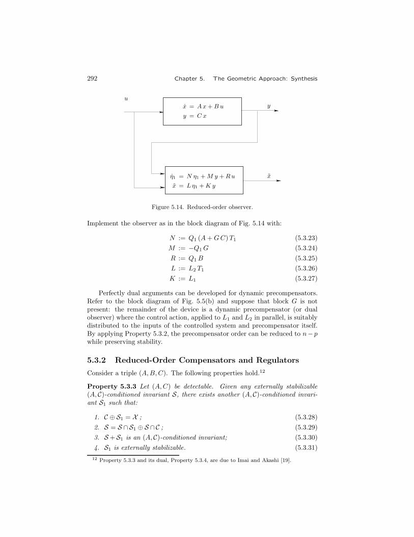
292 Chapter 5. The Geometric Approach: Synthesis
x = Ax+B u
y = C x
uy
xη1 = N η1 +M y +Ru
x = Lη1 +K y
Figure 5.14. Reduced-order observer.
Implement the observer as in the block diagram of Fig. 5.14 with:
N := Q1 (A+GC)T1 (5.3.23)
M := −Q1G (5.3.24)
R := Q1B (5.3.25)
L := L2 T1 (5.3.26)
K := L1 (5.3.27)
Perfectly dual arguments can be developed for dynamic precompensators.Refer to the block diagram of Fig. 5.5(b) and suppose that block G is notpresent: the remainder of the device is a dynamic precompensator (or dualobserver) where the control action, applied to L1 and L2 in parallel, is suitablydistributed to the inputs of the controlled system and precompensator itself.By applying Property 5.3.2, the precompensator order can be reduced to n− pwhile preserving stability.
5.3.2 Reduced-Order Compensators and Regulators
Consider a triple (A,B,C). The following properties hold.12
Property 5.3.3 Let (A,C) be detectable. Given any externally stabilizable(A, C)-conditioned invariant S, there exists another (A, C)-conditioned invari-ant S1 such that:
1. C ⊕ S1 = X ; (5.3.28)
2. S = S ∩S1 ⊕ S ∩C ; (5.3.29)
3. S +S1 is an (A, C)-conditioned invariant; (5.3.30)
4. S1 is externally stabilizable. (5.3.31)
12 Property 5.3.3 and its dual, Property 5.3.4, are due to Imai and Akashi [19].

5.3. Reduced-Order Devices 293
Property 5.3.4 Let (A,B) be stabilizable. Given any internally stabilizable(A,B)-controlled invariant V, there exists another (A,B)-controlled invariantV1 such that:
1. B ⊕ V1 = X ; (5.3.32)
2. V = V ∩V1 ⊕ V ∩B ; (5.3.33)
3. V ∩V1 is an (A,B)-controlled invariant; (5.3.34)
4. V1 is internally stabilizable. (5.3.35)
Proof of Property 5.3.4. Also this property is reconducted to Theorem5.3.2. The existence of a state feedback matrix F such that (A+BF )V1⊆V1and (A+BF )V ⊆V owing to Property 4.1.5 is equivalent to (5.3.34), whileconditions on spectra assignability, added to the assumptions that V is inter-nally stabilizable and (A,B) stabilizable, imply the possibility of A+BF beingstable, hence V1 internally stabilizable. �
It is now possible to state recipes for reduced-order compensators, assum-ing as the starting point those for full-order compensators presented in theprevious section. The only difference in computations is that, when derivingmatrices L1, L2 satisfying (5.2.18) in the case of the observer-based compen-sator or (5.2.54) in that of the dual observer-based compensator, it is assumedthat L :=S1 or L :=V1 (S1 and V1 are defined in Properties 5.3.3 and 5.3.4and G, F are determined in such a way that (A+GC)S1⊆S1, (A+GC)S ⊆Sand A+GC is stable in the former case, (A+BF )V1⊆V1, (A+BF )V ⊆V andA+BF is stable in the latter. In the proofs of the synthesis procedures only afew changes are needed: relations (5.2.19, 5.2.20) are replaced by (5.3.29, 5.3.28)above in the direct case, and (5.2.55) by (5.3.33, 5.3.32) in the dual one. Suit-able changes of basis, like that presented in the previous section for the reduced-order observer, allow elimination of n− q equations in the direct case and n− pequations in the dual one.
Observer-Based Reduced-Order Compensator. Given the resolventpair (S,V), determine L1, L2, F,G such that
1. L1C +L2= In , kerL2 =S1 ; (5.3.36)
2. (A+B F )V ⊆ V , A+BF is stable; (5.3.37)
3. (A+GC)S1 ⊆ S1 , (A+GC)S ⊆ S , A+GC is stable; (5.3.38)
then derive T1 and Q1 from T := [T1 T2], imT1= C, imT2 =S1 and
Q =
[Q1
Q2
]:= T−1
and realize the compensator according to
N := Q1 (A+GC + B F L2)T1 (5.3.39)
294 Chapter 5. The Geometric Approach: Synthesis
M := Q1 (B F L1 −G) (5.3.40)
L := F L2 T1 (5.3.41)
K := F L1 (5.3.42)
Dual Observer-Based Reduced-Order Compensator. Given theresolvent pair (S,V), determine L1, L2, F,G such that
1. BL1 +L2 = In , imL2 =V1 ; (5.3.43)
2. (A+B F )V1 ⊆ V1 , (A+B F )V ⊆ V , A+BF is stable; (5.3.44)
3. (A+GC)S ⊆ S , A+GC is stable. (5.3.45)
Then, derive T1 and Q1 from T := [T1 T2], imT1 =V1, imT2 =B, and
Q =
[Q1
Q2
]:= T−1
and realize the compensator according to
N := Q1 (A+B F + L2GC)T1 (5.3.46)
M := −Q1L2G (5.3.47)
L := (F + L1GC)T1 (5.3.48)
K := L1G (5.3.49)
We shall now consider the synthesis of reduced-order regulators. The onlydifference with respect to the compensators is that the pair (A,B) is notstabilizable; hence Theorem 5.3.2 is considered in its most general form throughthe following corollary.
Corollary 5.3.1 Consider a generic pair (A,B). Given an internally stableA-invariant P and an (A,B)-controlled invariant V such that V ∩P is inter-nally stabilizable, there exist both another (A,B)-controlled invariant V1 and amatrix F such that:
1. B ⊕ V1 = X ; (5.3.50)
2. V = V ∩V1 ⊕ V ∩B ; (5.3.51)
3. (A+BF )V1 ⊆ V1 ; (5.3.52)
4. (A+BF )V ⊆ V ; (5.3.53)
5. (A+BF )|P is stable; (5.3.54)
6. (A+BF )|X/V is stable. (5.3.55)
Proof. Consider Theorem [3.5.2] and determine V1 and F in such a way that(5.3.50–5.3.53) hold and all the free spectra are stabilized. Relation (5.3.55)holds since, V being externally stabilizable, V +R is externally stable bothas an A-invariant and an (A+BF )-invariant. V ∩P is an (A,B)-controlled in-variant (as the intersection of an (A,B)-controlled invariant and an A-invariant

5.4. Accessible Disturbance Localization and Model-Following Control 295
containing B), self-bounded with respect to V since V ∩B⊆V ∩P (as B⊆P).Restriction (A+BF )|(V∩P)/RV is stable because V ∩P is internally stabilizableand restriction (A+BF )|RV is stable because of the above choice of F ; hence(A+BF )|V∩P is stable. Since V is externally stable as an (A+BF )-invariant,it follows that (A+BF )|P is stable. �
We now present the recipes for regulators.
Observer-Based Reduced-Order Regulator. Given the resolventpair (S,V), determine L1, L2 still according to (5.3.36), while for F insteadof (5.3.37) consider the conditions:
2. (A+B F )V ⊆ V , (A+BF )|P is stable, (A+BF )|X/V is stable;(5.3.56)
and derive G still according to (5.3.38). Definitions of T1 and Q1 are the sameas in the compensator case. The regulator is defined again by (5.3.39–5.3.42).
Dual Observer-Based Reduced-Order Regulator. Given the re-solvent pair (S,V), determine L1, L2 still according to (5.3.43), while for F ,instead of (5.3.44), consider the conditions:
2. (A+B F )V1 ⊆ V1 , (A+B F )V ⊆ V , (A+BF )|P is stable,
(A+BF )|X/V is stable; (5.3.57)
and derive G still according to (5.3.45). Definitions of T1 and Q1 are the sameas in the compensator case. The regulator is defined again by (5.3.46–5.3.49).
5.4 Accessible Disturbance Localization and
Model-Following Control
We go back to the disturbance localization problem by dynamic compensator,already treated in Section 5.2, to give it a more general formulation. Refer tothe block diagram of Fig. 5.15, where disturbances (or nonmanipulable inputs)entering the controlled plant are two: an inaccessible disturbance d, and anaccessible disturbance d1.
The overall system, with extended state x := (x, z), is described by
˙x(t) = Ax(t) + D d(t) + R d1(t) (5.4.1)
e(t) = Ex(t) (5.4.2)
with
A :=
[A+BKC BL
MC N
]D :=
[DO
]
R :=
[D1 +BS
R
]E := [E O ]
(5.4.3)

296 Chapter 5. The Geometric Approach: Synthesis
y
d
x = Ax+B u+Dd+D1 d1
y = C x
e = E x
d1 e
u
x = N z +M y +Rd1
u = Lz +K y + S d1
Figure 5.15. Disturbance localization by dynamic compensation: dis-
turbances in part accessible.
Recalling the results of Section 4.2 on inaccessible disturbance localizationby dynamic output feedback and those of Section 5.2 on accessible disturbancelocalization by algebraic state feedback, we can give the problem the followinggeometric formulation.
Problem 5.4.1 (general disturbance localization by dynamic feedback) Referto the block diagram of Fig. 5.15 and assume that (A,B) is stabilizable and(A,C) detectable. Determine, if possible, a feedback compensator of the typeshown in the figure such that:
1. the overall system has an A-invariant W that satisfies
D ⊆ W ⊆ E , R ⊆ W (with R := imR )
2. A is stable.
Theorems 5.2.1 (nonconstructive conditions) and 5.2.2 (constructive con-ditions) can be extended to solve this more general problem. In the followingthe notation D1 := imD1 will be used.
Theorem 5.4.1 The disturbance localization problem by a dynamic compen-sator with disturbance in part accessible admits a solution if and only if thereexist both an (A,B)-controlled invariant V and an (A, C)-conditioned invariantS such that:
1. D ⊆ S ⊆ V ⊆ E ; (5.4.4)
2. D1 ⊆ V + B ; (5.4.5)
3. S is externally stabilizable; (5.4.6)
4. V is internally stabilizable. (5.4.7)

5.4. Accessible Disturbance Localization and Model-Following Control 297
Theorem 5.4.2 The disturbance localization problem by a dynamic compen-sator with disturbance in part accessible admits a solution if and only if
1. S∗ ⊆ V∗ ; (5.4.8)
2. D1 ⊆ V∗ + B ; (5.4.9)
3. SM is externally stabilizable; (5.4.10)
4. VM is internally stabilizable; (5.4.11)
5. V ′m := V∗ ∩minS(A, E ,B+D1) is internally stabilizable. (5.4.12)
Subspaces S∗,V∗,SM ,VM are defined by (5.1.57, 5.1.51, 5.1.73, 5.1.71).
Proof of Both Theorems. (hint) Necessity of (5.4.4–5.4.7) is proved as forTheorem 5.2.1, by projection of the conditions stated in the geometric formu-lation of the problem (in this case Problem 5.4.1); sufficiency of (5.4.4) and(5.4.6, 5.4.7) still as for Theorem 5.2.1, while sufficiency of (5.4.5) is proved asfollows: determine a dynamic compensator that realizes the inaccessible dis-turbance localization and denote by W the corresponding extended invariant.Since
D1 ⊆ W + B0 with D1 :=
[D1
O
]and B0 :=
[B OO Im
](5.4.13)
where, of course, D1 := imD1, B0 := imB0, is clearly possible to derive matricesR and S such that the corresponding R, defined in (5.4.3), satisfies the require-ment stated in Problem 5.4.1. As far as (5.4.12) is concerned, necessity followsfrom Property 4.1.5, while sufficiency is reduced to Theorem 5.4.1 by assumingS :=SM , V :=VM +V ′m as a resolvent pair. �
We shall now show that another well-known problem of control theory, themodel-following control , can be formally reduced to the accessible disturbancelocalization problem.13
This problem is stated in the following terms: refer to a completely con-trollable and observable three-map system, described by
xs(t) = As xs(t) +Bs us(t) (5.4.14)
ys(t) = Cs(t)xs(t) (5.4.15)
and suppose that a model , completely controllable, observable, and stable, isgiven as
xm(t) = Am xm(t) +Bm um(t) (5.4.16)
ym(t) = Cm(t)xm(t) (5.4.17)
The dimensions of the system and model output spaces are assumed to beequal.
13 Model-following systems were geometrically approached first by Morse [23].

298 Chapter 5. The Geometric Approach: Synthesis
ym
dynamiccompensator
xs = As xs +Bs us
ys = Cs xs
us ys
um xm = Am xm +Bm um
ym = Cm xm
Figure 5.16. Model-following compensator.
A control device is sought which, connected to the system and model asshown in Fig. 5.16, corresponds to a stable overall system and realizes thetracking of the model output, i.e., is such that, starting at the zero state and forall admissible input functions um(·), automatically provides a control functionus(·) which realizes equality ys(·)= ym(·).
This problem can be reduced to accessible disturbance localization bydynamic feedback and solved according to the block diagram shown in Fig. 5.15.To this end, assume
x :=
[xsxm
]u := us d1 := um (5.4.18)
and, for matrices
A :=
[As OO Am
]B :=
[Bs
O
]C := [Cs O ]
D :=
[OO
]D1 :=
[OBm
]E := [Cs −Cm ]
(5.4.19)
5.5 Noninteracting Controllers
Consider the block diagram of Fig. 5.1 and assume that the controlled system isstabilizable and detectable (i.e., that it coincides with the plant alone, withoutany exosystem). It is a five-map system (A,B,C,D,E), described by theequations:
x(t) = Ax(t) +B u(t) +Dd(t) (5.5.1)
y(t) = C x(t) (5.5.2)
e(t) = E x(t) (5.5.3)

5.5. Noninteracting Controllers 299
Suppose that a partition in k blocks of the controlled output e is given sothat by applying a suitable reordering of these components if needed, it is possi-ble to set e=(e1, . . . , ek); denote by E1, . . . , Ek the corresponding submatricesof E. A noninteracting controller is defined as follows.14
Definition 5.5.1 (noninteracting controller) The control apparatus of Fig. 5.1is said to be noninteracting with respect to partition (e1, . . . , ek) of output e ifthere exists a corresponding partition (r1, . . . , rk) of the reference input r suchthat, starting at the zero state, by acting on a single input ri (with all the otherinputs, d included, identically zero) only the corresponding output ei is changed,while the others remain identically zero.
The existence of a noninteracting controller for a given output partitionis strictly related to the system structure: in fact, noninteraction may involveloss of controllability if the system structure is not favorable. Noninteractionis clearly related to the concept of constrained controllability, introduced anddiscussed in Subsection 4.1.3. Let
Ei :=⋂j �=i
kerEi (i=1, . . . , k) (5.5.4)
It is clear that the reachable set on Ei, i.e.
REi = V∗i ∩minS(A, Ei,B) (i=1, . . . , k) (5.5.5)
with
V∗i := maxV(A,B, Ei) (i=1, . . . , k) (5.5.6)
is the maximal subspace on which, starting at the origin, state trajectories canbe obtained that affect only output ei, without influencing the other outputs,which remain identically zero.15
Therefore, conditions
EiREi = imEi (i=1, . . . , k) (5.5.7)
are necessary to perform a complete noninteracting control. They clearly de-pend on the system structure, hence are necessary whatever the type of con-troller used (for instance a nonlinear one). Necessary and sufficient conditionsfor the existence of a noninteracting control device implemented according tothe block diagram of Fig. 5.1 are stated in the following theorem.
14 The first geometric approaches to noninteracting controllers are due to Wonham andMorse [4.44, 24], and Basile and Marro [3]. We shall report here this latter treatment, whichis less general but more elementary and tutorial.
15 It is possible that, for one or more of the groups of output components required to be non-interacting, something more than simple controllability is preferred, for instance functionalcontrollability. If so, it is sufficient to replace REi
with FEi, the functional controllability
subspace on Ei, which can be computed by a suitable extension of the arguments presentedin Subsection 4.3.2. For specific treatment, see Basile and Marro [4].

300 Chapter 5. The Geometric Approach: Synthesis
Theorem 5.5.1 Refer to a quintuple (A,B,C,D,E) with (A,B) stabilizableand (A,C) detectable. Given a partition (e1, . . . , ek) of the controlled outputvariables, there exists a noninteracting control device of the type shown inFig. 5.1 if and only if conditions (5.5.7) hold.
Proof. Only if. This part of the proof is directly implied by the concept ofconstrained controllability.
If. Consider the extended mathematical model
˙x(t) = A x(t) + D d(t) + R r(t) (5.5.8)
e(t) = E x(t) (5.5.9)
where matrices are the same as in (5.1.12). Owing to Theorem 3.3.1 oncontrollability, system (5.5.8–5.5.9) is noninteracting if and only if:
R∗i ⊆⋂j �=i
kerEj (i=1, . . . , k) (5.5.10)
Ei R∗i = imEi (i=1, . . . , k) (5.5.11)
where R∗i :=minJ (A, imRi) and Ri, Ei denote the submatrices of R and
E corresponding, respectively by columns and rows, to the above-mentionedpartitions of r and e. To prove sufficiency, we shall perform the synthesis of alinear compensator satisfying (5.5.10, 5.5.11) and such that matrix A is stable.
+
+
+
+
u1 u er1
r2
rk
u2
uk
z1 = N1 z1 +R1 r1
u1 = L1 z1 + S1 r1
z2 = N2 z2 +R2 r2
u2 = L2 z2 + S2 r2
zk = Nk zk +Rk rk
uk = Lk zk + Sk rk
x = Ax+B u
e = E x
Figure 5.17. Realizing a noninteracting controller by means of k dy-
namic precompensators.
For this, refer to the simplified scheme of Fig. 5.17 (where d and y have beentemporarily ignored) and suppose, for a moment, that A is a stable matrix: this

5.5. Noninteracting Controllers 301
assumption will be removed later. For each ei (i=1, . . . , k) realize an identitydynamic precompensator of the type shown in Fig. 3.12(c) and express itsstate in the basis defined by similarity transformation Ti := [Ti,1 Ti,2] withimTi,1=REi , and input in the basis defined by transformation Ui := [Ui,1 Ui,2]with im(BUi,1)=V∗i ∩B, im(BUi)=B. The system equations become
A′i := T−1i ATi =
[A′i,11 A′i,12A′i,21 A′i,22
]B′i := T−1i B Ui =
[B′i,11 OO B′i,22
](5.5.12)
with (A′i,11, B′i,11) controllable. Hence, there exists at least one matrix
F ′i :=
[F ′i,11 OF ′i,21 O
](5.5.13)
such that A′i,11 +B′i,11F′i,11 is stable and A′i,21 +B′i,22F
′i,21 a zero matrix. In the
new basis the identity dynamic precompensator is described by the equations[zi,1(t)zi,2(t)
]=
[A′i,11 +B′i,11F
′i,11 A′i,12
O A′i,22
] [zi,1(t)zi,2(t)
]+
[B′i,11 OO B′i,22
] [ri,1(t)ri,2(t)
](5.5.14)
Note that the components of zi,2 belong to kerF ′i and that to obtain nonin-teraction it is in any case necessary to assume ri,2(·)= 0, so that it is possibleto ignore these components in the actual realization of the device. Hence, weassume zi := zi,1, ri := ri,1 and
Ni := A′i,11 +B′i,11 F′i,11 (5.5.15)
Ri := B′i,11 (5.5.16)
Li := Ui,1 F′i,11 (5.5.17)
Si := Ui,1 (5.5.18)
The order of the obtained precompensator is clearly equal to dimREi .
++
y
v2
x = Ax+B u+Dd
y = C x
e = E x
d e
v1
z = N z +M y + v2
u = Lz +K y
u
Figure 5.18. Stabilizing the plant.
We shall now remove the assumption that matrix A is stable. Should A notbe stable, there would exist a dynamic feedback of the type shown in Fig. 5.18

302 Chapter 5. The Geometric Approach: Synthesis
so that the corresponding extended system is stable. This is described by
˙x(t) = (A0 + B0KC0) x(t) + B0 u(t) + D d(t) (5.5.19)
y(t) = C0 x(t) (5.5.20)
e(t) = E x(t) (5.5.21)
where
u :=
[v1v2
]
and A0, B0, C0, D, E, K are the same as in (5.1.18, 5.1.19).Owing to Lemma 5.1.1, subspaces
V∗i :=
{[xz
]: x ∈ V∗i , z = T x
}(i=1, . . . , k) (5.5.22)
where T denotes an arbitrary suitably dimensioned matrix, are (A0, B0)-controlled invariants, hence (A0 + B0KC0, B0)-controlled invariants, since feed-back through input does not influence controlled invariance (the arbitrarinessof T depends on the forcing action of the stabilizing unit being completelyaccessible). The reachable sets on them are
REi ={[
xz
]: x ∈ REi , z = T x
}(i=1, . . . , k) (5.5.23)
and clearly have the same dimensions as the reachable sets REi (i=1, . . . , k)in the nonextended state space.
Therefore, this procedure can be applied referring to the extended system(controlled system and stabilizing feedback unit), without any change in thestate dimensions of the dynamic precompensators. A straightforward checkshows that the extended system (5.5.8, 5.5.8), which is clearly stable, satisfiesthe noninteraction conditions (5.5.10, 5.5.11). �
Obtaining Stability, Disturbance Localization, and Noninterac-tion Simultaneously. Disturbance d has not been considered in the previ-ous proof. Indeed, due to linearity and superposition property, it can be han-dled completely independently of noninteraction: if the necessary and sufficientconditions stated in Theorems 5.2.1 and 5.2.2 (when disturbance is completelyinaccessible), or in Theorems 5.4.1 and 5.4.2 (when disturbance is in part ac-cessible), are satisfied, a stabilizing dynamic unit of the type shown in Fig. 5.18can be used to provide also disturbance localization. Since controlled invariantsof the extended system are preserved in the presence of any through-input feed-back, the possibility of simultaneously achieving noninteraction is not affectedby the actual values of the dynamic compensator matrices K,L,M,N .
The solution to the noninteracting control problem presented in the proof ofTheorem 5.5.1 is completely exhaustive, since it realizes noninteraction when-ever all the necessary and sufficient conditions are met. However it is not

5.5. Noninteracting Controllers 303
claimed here to be the most convenient with respect to robustness in the pres-ence of parameter changes and/or uncertainty, and the minimal with respectto the regulator order. On the contrary, its order appears to be relatively highin comparison with other regulation problems (where the order of the con-troller coincides, at most, with that of the controlled system). This happensbecause the intersections of controlled invariants REi in general are not con-trolled invariants themselves, so that it is not possible to achieve noninteractionby means of state feedback through a unique asymptotic state observer.

304 Chapter 5. The Geometric Approach: Synthesis
References
1. Akashi, H., and Imai, H., “Disturbance localization and output deadbeatcontrol through an observer in discrete-time linear multivariable systems,” IEEETrans. Autom. Contr., vol. AC-24, pp. 621–627, 1979.
2. Antoulas, A.C., “A new approach to synthesis problems in linear systemtheory,” IEEE Trans. Autom. Contr., vol. AC-30, no. 5, pp. 465–473, 1985.
3. Basile, G., and Marro, G., “A state space approach to noninteractingcontrols,” Ricerche di Automatica, vol. 1, no. 1, pp. 68–77, 1970.
4. — , “On the perfect output controllability of linear dynamic systems,” Ricerchedi Automatica, vol. 2, no. 1, pp. 1–10, 1971.
5. — , “Dual-lattice theorems in the geometric approach,” J. Optimiz. Th. Applic.,vol. 48, no. 2, pp. 229–244, 1986.
6. Basile, G., Marro, G., and Piazzi, A., “Stability without eigenspaces inthe geometric approach: some new results,” Frequency Domain and State SpaceMethods for Linear Systems, edited by C. A. Byrnes and A. Lindquist, North-Holland (Elsevier), Amsterdam, pp. 441–450, 1986.
7. — , “Revisiting the regulator problem in the geometric approach. Part I.Disturbance localization by dynamic compensation,” J. Optimiz. Th. Applic., vol.53, no. 1, pp. 9–22, 1987.
8. — , “Revisiting the regulator problem in the geometric approach. Part II.Asymptotic tracking and regulation in the presence of disturbances,” J. Optimiz.Th. Applic., vol. 53, no. 1, pp. 23–36, 1987.
9. — , “Stability without eigenspaces in the geometric approach: the regulatorproblem,” J. Optimiz. Th. Applic., vol. 64, no. 1, pp. 29–42, 1990.
10. Bhattacharyya, S.P., “Disturbance rejection in linear systems,” Int. J. Sys-tems Science, vol. 5, no. 7, pp. 633–637, 1974.
11. — , “Frequency domain condition for disturbance rejection,” IEEE Trans. Au-tom. Contr., vol. AC-25, no. 6, pp. 1211–1213, 1980.
12. — , “Frequency domain condition for output feedback disturbance rejection,”IEEE Trans. Autom. Contr., vol. AC-27, no. 4, pp. 974–977, 1982.
13. Bhattacharyya, S.P., Pearson, J.B., and Wonham, W.M., “On ze-roing the output of a linear system,” Information and Control , vol. 20, no. 2, pp.135–142, 1972.
14. Brash, F.M., and Pearson, J.B., “Pole placement using dynamic compen-sators,” IEEE Trans. Autom. Contr., vol. AC-15, no. 1, pp. 34–43, 1970.
15. Chang, M.F., and Rhodes, I.B., “Disturbance localization in linear systemswith simultaneous decoupling, pole assignment, or stabilization,” IEEE Trans.Autom. Contr., vol. AC-20, pp. 518–523, 1975.
16. Cheng, L., and Pearson, J.B., “Frequency domain synthesis of multivariablelinear regulators,” IEEE Trans. Autom. Contr., vol. AC-23, no. 1, pp. 3–15, 1978.
17. Francis, B.A., “The multivariable servomechanism problem from the input-output viewpoint,” IEEE Trans. Autom. Contr., vol. AC-22, no. 3, pp. 322–328,1977.
References 305
18. Hamano, F., and Furuta, K., “Localization of disturbances and outputdecomposition in decentralized linear multivariable systems,” Int. J. Control , vol.22, no. 4, pp. 551–562, 1975.
19. Imai, H., and Akashi, H., “Disturbance localization and pole shifting by dy-namic compensation,” IEEE Trans.tss Autom.Contr., vol. AC-26, no. 1, pp. 226–235, 1981.
20. Kucera, V., “Discrete linear model following systems,” Kybernetika (Praga),vol. 13, no. 5, pp. 333–342, 1977.
21. — , “Disturbance rejection: a polynomial approach,” IEEE Trans. Autom.Contr., vol. AC-28, no. 4, pp. 508–511, 1983.
22. Marro, G., and Piazzi, A., “Duality of reduced-order regulators,” Proceed-ings of the ’88 International AMSE Conference on Modelling and Simulation,Istambul, 1988.
23. Morse, A.S., “Structure and design of linear model following systems,” IEEETrans. Autom. Contr., vol. AC-18, no. 4, pp. 346–354, 1973.
24. Morse, A.S., and Wonham, W.M., “Decoupling and pole assignment bydynamic compensation,” SIAM J. Control , vol. 8, no. 3, pp. 317–337, 1970.
25. Ohm, D., Bhattacharyya, S.P., and Houze, J.W., “Transfer matrixconditions for (C,A,B)-pairs,” IEEE Trans. Autom. Contr., vol. AC-29, pp. 172–174, 1984.
26. Ozguler, A.B., and Eldem, V., “Disturbance decoupling problems viadynamic output feedback,” IEEE Trans. Autom. Contr., vol. AC-30, pp. 756–764, 1986.
27. Piazzi, A., “Pole placement under structural constraints,” IEEE Trans. onAutomatic Control , vol. 35, no. 6, pp. 759–761, 1990.
28. — , “Geometric aspects of reduced-order compensators for disturbance rejection,”IEEE Trans. on Automatic Control , vol. 36, no. 1, pp. 102–106, 1991.
29. Piazzi, A., and Marro, G., “The role of invariant ze-ros in multivariable system stability,” Proceedings of the1991 European Control Conference, Grenoble, 1991.
30. Schumacher, J.M.H., “Compensator synthesis using (C,A,B)-pairs,” IEEETrans. Autom. Contr., vol. AC-25, no. 6, pp. 1133–1138, 1980.
31. — , “Regulator synthesis using (C,A,B)-pairs,” IEEE Trans. Autom. Contr.,vol. AC-27, no. 6, pp. 1211–1221, 1982.
32. — , “The algebraic regulator problem from the state-space point of view,” LinearAlgebra and its Applications, vol. 50, pp. 487–520, 1983.
33. — , “Almost stabilizability subspaces and high gain feedback,” IEEE Trans.Autom. Contr., vol. AC-29, pp. 620–627, 1984.
34. Shah, S.L., Seborg, D.E., and Fisher, D.G., “Disturbance localizationin linear systems by eigenvector assignment,” Int. J. Control , vol. 26, no. 6, pp.853–869, 1977.
35. Willems, J.C., “Almost invariant subspaces: an approach to high gain feed-back design - Part I: Almost controlled invariant subspaces,” IEEE Trans. Autom.Contr., vol. AC-26, no. 1, pp. 235–252, 1981.
36. Willems, J.C., “Almost invariant subspaces: an approach to high gain feed-back design - Part II: Almost conditionally invariant subspaces,” IEEE Trans.Autom. Contr., vol. AC-27, no. 5, pp. 1071–1085, 1982.

306 Chapter 5. The Geometric Approach: Synthesis
37. Willems, J.C., and Commault, C., “Disturbance decoupling by measure-ment feedback with stability or pole placement,” SIAM J. Contr. Optimiz., vol.19, no. 4, pp. 490–504, 1981.
38. Wonham, W.M., “Dynamic observers – geometric theory,” IEEE Trans. Au-tom. Contr., vol. AC-15, no. 2, pp. 258–259, 1970.
39. — , “Tracking and regulation in linear multivariable systems,” SIAM J. Control ,vol. 11, no. 3, pp. 424–437, 1973.
40. Wonham, W.M., and Pearson, J.B., “Regulation and internal stabilization
in linear multivariable systems,” SIAM J. Control , vol. 12, no. 1, pp. 5–18, 1974.

Chapter 6
The Robust Regulator
6.1 The Single-Variable Feedback Regulation
Scheme
In this chapter the robust multivariable regulator will be investigated by usingthe geometric approach techniques presented in Chapters 3, 4, and 5. A regu-lator is said to be robust if it preserves the regulation property and satisfactorydynamic behavior also in the presence of variations of the parameters of theplant in well-defined neighborhoods of their nominal values, called uncertaintydomains . These parameter variations are assumed to be “slow” with respectto the most significant time constants of the controlled plant, so that theirinfluence on the controlled output is negligible if the regulation property ismaintained for all the parameter values.
Many basic concepts of the standard single-variable regulator design tech-niques will be revisited with a different language and extended to the multi-variable case. For better understanding and framing of this connection in lightof the traditional approach, in this first section the most important terms andconcepts of automatic control theory will be briefly recalled and a short sketchof the standard synthesis philosophy will be discussed.
Refer to the block diagram of Fig. 6.1. It is well known that in standardsingle-variable systems robustness is achieved by using feedback, i.e., by feedingback to the controller a measurement of the controlled output (which mustbe as accurate as possible) or, more exactly, through very accurate directdetermination of the tracking error variable, which is a known, simple functionof the controlled output.
The meanings of the symbols in the figure are:
r: reference input
e: error variable
m: manipulable input
d: disturbance input
c: controlled output
y1, y2: informative outputs
307

308 Chapter 6. The Robust Regulator
The informative outputs are in general stabilizing signals: a typical exampleis the tachymetric feedback in position control systems.
+_
+
+
exosystem 1
R(s)r e
Gc(s)m
G(s)
D(s)
regulator plant
de
exosystem 2
y1 y2
Figure 6.1. A feedback control system.
We shall now consider the particular case
G(s) :=1
(s+ a) (s+ b) (s+ c)R(s) =
1
s2D(s) =
1
s(6.1.1)
The displayed functions are “generalized transfer functions”: in the case ofthe exosystems the inputs are understood to be identically zero, so that thecorresponding outputs are affected only by the initial conditions. Our aim isto determine a Gc(s) such that the extended plant (i.e., the plant plus theregulator) is (asymptotically) stable and the overall system (i.e., the extendedplant plus the exosystems) satisfies the regulation condition limt→∞ e(t) = 0.Note that the exosystems are (asymptotically) unstable and introduce into theextended plant signals of the general type
μ+ ν t
whose coefficients μ and ν depend on the initial conditions of the exosystems.This problem can be reformulated in the state space. Consider the signal-
flow graph of Fig. 6.2(a), derive the equivalent graph of Fig. 6.2(b) (wherethe second exosystem, which is not independently observable from output e, isembedded in the first), and define a state variable for every integrator as shownin the figure: we derive the state space representation
A =
⎡⎢⎢⎢⎣−a 0 0 0 01 −b 0 0 00 1 −c 0 00 0 0 0 10 0 0 0 0
⎤⎥⎥⎥⎦ B =
⎡⎢⎢⎢⎣10000
⎤⎥⎥⎥⎦ D =
⎡⎢⎢⎢⎣00000
⎤⎥⎥⎥⎦
C = E = [ 0 0 −1 −k 1 ]
(6.1.2)

6.1. The Single-Variable Feedback Regulation Scheme 309
1
1
1
111
1
1111
s−1s−1
s−1s−1s−1
s−1s−1
s−1
s−1s−1s−1
− a
− a
− b
− b − c
− c
m ≡ u
m ≡ u
k
k
c
e
e
plant
plant
−1
−1
exosystem 2
exosystem 1
exosystem
x1 x2 x2 x3 x3 ≡ c
x5
x5 ≡ d x4 x4 ≡ r
x1
(a)
(b)
Figure 6.2. Signal-flow graph representations of a controlled system.
Note that in this case the informative and controlled outputs coincide.A traditional design is developed according to the following steps: since theexosystem introduces observable unstable modes, the regulator must generateidentical modes so that the steady state error is zero. In other words, a model ofthe exosystem must be contained in the regulator. This expresses the so-calledinternal model principle, which corresponds to a design expedient that is wellknown in the single-variable case: to achieve zero steady state error in the stepresponse, the regulator must have a pole at the origin, like the exosystem thatgenerates the step, while the same requirement for the ramp response impliesa double pole at the origin, and so on. For the sake of generality we assume
Gc(s) :=γ (s+ α) (s+ β)
s2(6.1.3)
In this way the maximum number of zeros compatible with the physical realiz-ability or causality condition (the degree of the numerator must be less than,

310 Chapter 6. The Robust Regulator
or equal to that of the denominator) is inserted into the regulator: the values ofparameters α, β, γ are free and can be chosen to achieve stability and improvethe transient behavior of the loop, if possible. If stability is not achievableor the transient behavior cannot be made completely satisfactory, significantimprovements can be generally obtained by inserting some further pole-zeropairs into the regulator.
A realization of the regulator described by transfer function (6.1.3) isrepresented in Fig. 6.3. From the signal-flow graph one immediately derivesthe quadruple
K := γ L := [β α ] M :=
[γγ
]N :=
[0 α0 0
](6.1.4)
which completes the state space representation of the type shown in Fig. 5.3.
11
1 s−1s−1γ
x2 x2 m ≡ ux1 x1
α β
e
Figure 6.3. Signal-flow graph representation of a possible feedback regulator.
The state-space solution of the multivariable regulator problem will bedescribed in the next section. Let us now list and explain the most significantsteps of the traditional synthesis by assuming the previous example as referencebut trying to derive general results, which will be extended to the multivariablecase.
Robust Stability. In the case of the previous example, the typicalsituation that can be referred to when coefficients a, b, c are nonnegative andα, β, γ positive is illustrated by the root locus shown in Fig. 6.4: the system issurely stable for a proper choice of the gain γ if the absolute values of a, b, care large with respect to those of α, β.
If all the exosystem poles are located at the origin (as in the most commoncases) this condition is met if sufficiently small α and β are chosen; however,by so doing, the poles that originate from the exosystem are maintained veryclose to the origin, and this causes a very slow transient. In any case it isconvenient to translate the poles of the plant toward the left by inserting in theregulator some pole-zero pairs or by means of feedback connections using theinformative outputs: since the plant is completely controllable and observable,its poles are all arbitrarily assignable, at least with a proper state observer witharbitrary poles. If the plant is minimum-phase, i.e., has all the poles and zeroswith the real parts negative, a robust stability is always possible. If the planthas some poles and zeros with the real parts positive it is still pole assignable,hence stabilizable, by means of a suitable dynamic feedback connection, butthe root locus corresponding to this feedback, which originates and terminatesin the right half-plane is, in general, very sensitive to parameter changes in its

6.1. The Single-Variable Feedback Regulation Scheme 311
x x x xx
ω
− b
− a − c −α − β 0 σ
Figure 6.4. Root locus of system (6.1.1) and regulator (6.1.3).
stable portion and remains in the left half-plane for a very short gain interval,so that robust stability is very difficult to achieve.
Observability and the Internal Model. In the preceding example themode generated by the second exosystem (a step) is a part of those generatedby the first one (a step and a ramp), so that it is not necessary to reproduceboth exosystems in the regulator; in fact a double pole at the origin allowssteady state compensation of any set of disturbances consisting of a linearcombination of a step and a ramp, independently of the points where theyare introduced in the regulation loop. The reason it is possible to use a singleinternal model in this case is that the exosystems that generate the disturbancesare not all separately observable from the controlled output e, so that it issufficient to reproduce in the regulator only the eigenstructures correspondingto the observable exogenous modes. In the single-variable case it is generallyconvenient to assume in the mathematical model a single exosystem which iscompletely observable [as was obtained by replacing the signal-flow graph ofFig. 6.2(a) with that of Fig. 6.2(b), but this may not apply to the multivariablecase where a single exosystem that influences several regulated outputs cannotbe compensated by a single internal model if coefficients of influence are subjectto changes, resulting in lack of robustness. This point, which represents animportant difference between the single-variable and the multivariable case,will be thoroughly investigated in the Section 6.3.
Robust Regulation. In the single-variable case, regulation is robustversus parameter variations provided the plant remains stable and the internalmodel is preserved when coefficients change. As previously mentioned, if theplant pole-zero configuration is favorable, the plant stability requirement canbe robustly satisfied by suitable placement of the free poles and zeros. It is not

312 Chapter 6. The Robust Regulator
difficult to build a robust internal model if the exogenous eigenvalues are allzero: fortunately this case is very frequent in practice since specifications onregulator asymptotic behavior usually refer to test signals consisting of steps,ramps, parabolas, and so on. However, in the multivariable case it is furthernecessary that individual asymptotic controllability of regulated outputs fromthe plant inputs is maintained in the presence of parameter variations. Thisstructural requirement is another important point that distinguishes the mul-tivariable from the single-variable case.
6.2 The Autonomous Regulator: A General
Synthesis Procedure
In the regulator problem formulated in Section 5.2, two types of input functionswere considered: an input function d(·) belonging to a very general class (thatof bounded and piecewise continuous functions), representing a nonmanipulableinput to be identically localized, i.e., to be made noninfluencing of the controlledoutput at any time through a suitable change of structure, and an inputfunction x2(·), generated by an exosystem, of a more particular class (thatof the linear combinations of all possible modes of a linear time-invariantsystem), representing a nonmanipulable input to be asymptotically localized.This formulation of the problem has the advantage of being very general: forinstance, it extends in the most natural way a classic geometric approachproblem, i.e., disturbance localization through state feedback.
When robustness is a required regulator feature, “rigid” solutions like thestandard structural disturbance localization are not acceptable since, in gen-eral, they lose efficiency in the presence of parametric variations; therefore itis necessary to have to resort to “elastic” solutions like the asymptotic insen-sitivity to disturbances modeled by an exosystem. Note that if the controlledoutput dynamics is sufficiently fast (or even arbitrarily fast, i.e., with arbitrar-ily assignable modes), this approach is almost equivalent to rigid localizationsince the localization error corresponding to a disturbance signal with limitedbandwidth can be made arbitrarily small.
In light of these considerations we shall first of all see how the statementsof Theorems 5.2.2 and 5.2.4 simplify on the assumption that D=O, i.e., whenan autonomous regulator is considered. In this case the overall system is notsubject to any external signal, since the only considered perturbations are thoseof the initial states (of the plant, exosystem, and regulator): it is requiredthat for any set of initial states the regulation condition limt→∞ e(t)= 0 ismet. This formulation is the direct extension of that presented in the previoussection for single-variable systems. It is worth pointing out that the robustnessrequirement will not be considered in this section. The conditions that arederived as particular cases of those considered in Section 5.2 are necessaryand sufficient for the existence of a generic, stable autonomous regulator, butdo not guarantee the existence of an autonomous regulator of the feedback

6.2. The Autonomous Regulator: A General Synthesis Procedure 313
type (it may be feedforward). Hence, they are only necessary to extend tomultivariable systems the synthesis procedure for robust regulators (based onfeedback through an internal model of the exosystem) illustrated in the previoussection for the single-variable case.
u
y
x2 = A2 x2
x1 = A1 x1 + A3 x2 +B1 u
e = E1 x1 + E2 x2
y = C1 x1 + C2 x2
x2
controlled system
e
x = N z +M y
u = Lz +K yregulated plant
exosystem
regulator
plant
Figure 6.5. The general multivariable autonomous regulator.
For the sake of clarity and to make this chapter self-contained, it appearsconvenient to report first a specific formulation of the autonomous regulatorproblem. Consider the overall system represented in Fig. 6.5, whose stateevolution is described by the homogeneous matrix differential equation⎡
⎣ x1(t)x2(t)z(t)
⎤⎦ =
⎡⎣A1 +B1KC1 A3 +B1KC2 B1L
O A2 OMC1 MC2 N
⎤⎦
⎡⎣ x1(t)x2(t)z(t)
⎤⎦ (6.2.1)
which, according to the notation introduced in Section 5.1, can also be written,together with the output equation, in the compact form
˙x(t) = A x(t)
e(t) = E x(t)with A :=
[A1A3
A4A2
]and E := [E1 O] (6.2.2)
i.e., as a unique extended system with the submatrices of A and E defined by
A1 :=
[A1 +B1KC1 A3 +B1KC2
O A2
]A3 :=
[B1LO
]
A4 := [MC1 MC2 ] A2 := N E1 := E = [E1 E2 ]
(6.2.3)

314 Chapter 6. The Robust Regulator
The part of the overall system driven by the exosystem is called the reg-ulated plant (the plant plus the regulator): it has x2 as the only input ande as the only output and is a nonpurely dynamic system represented by thequadruple (Ap, Bp, Cp, Dd) with
Ap :=
[A1 +B1KC1 B1L
MC1 N
]Bp :=
[A3 +B1KC2
MC2
]
Cp := [E1 O ] Dp := [E2 ]
(6.2.4)
As the last step of this review of the new and old notations, recall the fourremaining matrices of the five-map controlled system, which are the only dataprovided to solve our regulation problem:
A :=
[A1 A3
O A2
]B :=
[B1
O
]C := [C1 C2 ] E := [E1 E2 ] (6.2.5)
We shall denote with n1 the state dimension of the plant, with n2 that ofthe exosystem, and with m that of the regulator; the plant , and the extendedplant defined by (5.1.8) and (5.2.7) are respectively an A-invariant and an A-invariant which in the above considered coordinate systems can be expressedas
P = imP with P :=
[In1
O
](6.2.6)
and
P = imP with P :=
⎡⎣ In1 OO OO Im
⎤⎦ (6.2.7)
In the autonomous regulator case the plant stability condition simply meansthat the regulated plant must be stable, i.e., that Ap must be a stable matrix or
that P must be internally stable as an A-invariant, and the regulation conditionmeans that there exists an externally stable A-invariant contained in kerE.Geometrically the autonomous regulator problem is stated in the followingterms, as a particular case of Problem 5.2.4.
Problem 6.2.1 Refer to the block diagram of Fig. 6.5 and assume that(A1, B1) is stabilizable and (A,C) detectable. Determine, if possible, a feed-back regulator of the type shown in the figure such that:
1. the overall system has an A-invariant W that satisfies
W ⊆ E with E := kerE ;
2. W is externally stable;
3. W ∩ P (which is an A-invariant) is internally stable.

6.2. The Autonomous Regulator: A General Synthesis Procedure 315
The elimination of input D significantly simplifies the necessary and suffi-cient conditions stated in Chapter 5. In fact, from D := imD= {0} it followsthat S∗=Sm =SM = {0}; hence
Vm = VM = V∗ ∩minS(A, E ,B) = RV∗ = RE (6.2.8)
so that from Theorems 5.2.2 and 5.2.4 the following corollaries are immediatelyderived.
Corollary 6.2.1 The autonomous regulator problem has a solution if and onlyif there exists an (A,B)-controlled invariant V such that:
1. V ⊆ E ; (6.2.9)
2. V is externally stabilizable; (6.2.10)
3. V ∩P is internally stabilizable. (6.2.11)
Corollary 6.2.2 Let all the exogenous modes be unstable. The autonomousregulator problem has a solution if and only if:
1. V∗ is externally stabilizable; (6.2.12)
2. V∗ ∩P is complementable with respect to (RV∗ ,V∗) . (6.2.13)
At this point some remarks are in order.
1. Due to the particular structure of matrix A, the assumption that (A,C) isdetectable clearly implies that (A1, C1) also is.
2. Let all the exogenous modes be unstable. For the regulator problem tohave a solution, as a clear consequence of (6.2.12) it is necessary that
imE2 ⊆ imE1 (6.2.14)
3. Condition (6.2.12 ) can be reformulated in the very strict geometric way
V∗ + P = X (6.2.15)
In fact it has been previously proved (point e of the proof of Theorem 5.2.4)that if V is any (A,B)-controlled invariant self-bounded with respect to V∗ theinternal unassignable eigenvalues in between V ∩P and V are all exogenous.This property, applied to V∗ itself, clearly implies (6.2.15).
These conditions hold also in the general case considered in Chapter 5, buthave not been mentioned before, since they are straightforward consequencesof the assumptions or of the derived geometric conditions.
We shall now derive an important theorem (Theorem 6.2.1) which setsa further, significant simplification of the necessary and sufficient conditions(6.2.15, 6.2.13) and provides a basic means to approach structural robustness inthe multivariable regulator case. First, we state a property that geometricallycharacterizes any solution of the problem.
316 Chapter 6. The Robust Regulator
Property 6.2.1 Let all the exogenous modes be unstable. The regulator corre-sponding to the overall system matrices A, E satisfies both plant stability and theregulation condition if and only if there exists an externally stable A-invariantW such that:
1. W ⊆ E with E := kerE; (6.2.16)
2. W ⊕ P = X . (6.2.17)
Proof. Only if. The plant stability condition means that P is internallystable as an A-invariant and the regulation condition holds if and only ifthere exists an externally stable A-invariant contained in E . Denote this byW1. Since the eigenvalues of A2, i.e., the eigenvalues of the exosystem (whichhave been assumed to be unstable) are a part of those of A, they must beinternal eigenvalues of W1. By reason of dimensionality the other eigenvaluesof A coincide with those of Ap so that the A-invariant W1 ∩ P is internally
stable and P is complementable with respect to (W1 ∩ P, W1). Assume thesimilarity transformation T := [T1 T2 T3], with imT1= W1 ∩ P, im [T1 T2] = W1,im [T1 T3] = P . In the new basis, A′ :=T−1AT and E′ := ET have the structures
A′ =
⎡⎣A′11 A′12 A′13O A′22 OO O A′33
⎤⎦ E′ = [O O E′3 ] (6.2.18)
Matrices A′11 and A′33 are stable while A′22 is unstable, so that the Sylvesterequation
A′11X −X A′22 = −A′12 (6.2.19)
admits a unique solution X . Define W as the image of T1X +T2. Clearly itsatisfies both the conditions in the statement.
If. The regulation condition is satisfied since W attracts all the externalmotions. Furthermore, W has the eigenvalues of A2 as the only internaleigenvalues and those of the regulated plant as the only external ones, so thatthe plant stability condition is satisfied. �
For those who like immediate translation of geometric conditions into ma-trix equations, we can state the following corollary.
Corollary 6.2.3 Let all the exogenous modes be unstable and suppose that theregulated plant is stable. The regulation condition is satisfied if and only if theequations
ApXp −XpA2 = −Bp (6.2.20)
CpXp +Dp = O (6.2.21)
have a solution in Xp.

6.2. The Autonomous Regulator: A General Synthesis Procedure 317
Proof. The complementability condition implies the possibility of assuming
W := im(⎡⎣X1
In2
Z
⎤⎦)
with
[X1
Z
]= Xp (6.2.22)
From Property 3.2.1 it follows that the equations (6.2.20, 6.2.21) are satisfiedif and only if W is an A-invariant contained in E. �
As in the case of the general regulator problem approached in Chapter 5,necessary and sufficient conditions referring to the overall system and expressedin terms of invariants, reflect in necessary and sufficient conditions referringto the sole controlled system and expressed in terms of controlled and/orconditioned invariants. These conditions are directly usable for feasibilitychecks and for constructive synthesis procedures. The basic result is statedin the following theorem whose proof, although contained in that of Theorem5.2.4, is developed here in a completely self-contained way.
Theorem 6.2.1 (the fundamental theorem on the autonomous regulator) Letall the exogenous modes be unstable. The autonomous regulator problem admitsa solution if and only if there exists an (A,B)-controlled invariant V such that
1. V ⊆ E ; (6.2.23)
2. V ⊕ P = X . (6.2.24)
Proof. Only if. Consider the A-invariant W defined by (6.2.22) and denoteby W the corresponding basis matrix, also shown in (6.2.22): by Property 3.2.1there exists a matrix X such that AW = W X . Straightforward manipulationsshow that this equation implies the existence of a matrix U such that
A
[X1
In2
]= X
[X1
In2
]+B U
Hence
V :=
[X1
In2
]
is an (A,B)-controlled invariant by Property 4.1.4. It clearly satisfies both thestated conditions.
If. We prove that the conditions in the statement imply those of Corollary6.2.1. Condition (6.2.9) holds by assumption. Condition (6.2.10) is provedas follows: the A-invariant V +P , which covers the whole space, is externallystable [hence, in particular, externally stabilizable as an (A,B)-invariant], sothat V is externally stabilizable (see point f of the proof of Theorem 5.2.4).Finally, (6.2.11) is implied by V ∩P = {0}. �
This proof of the fundamental theorem is the most direct in connectionwith the previously developed theory. Another proof, which has the advantage

318 Chapter 6. The Robust Regulator
of being completely constructive, can be based on Algorithm 6.2.1 (for the onlyif part) and Algorithm 6.2.3 (for the if part).
Note that the controlled invariant V considered in the statement has thedimension equal to that of the exosystem, so that its unique internal eigen-values (clearly unassignable) coincide with those of the exosystem. Since anyresolvent must have the eigenvalues of the exosystem as internal, since it mustbe externally stabilizable, V is a minimal-dimension resolvent . It will be shownin Section 6.4 that having a minimal-dimension resolvent is a basic step for thesynthesis of a particular multivariable robust feedback regulator that is alsominimal-dimension.
Given the data of our problem, i.e., matrices A,B,C,E, the conditionsof Corollary 6.2.1 can be checked in a completely automatic way through thecomputation of V∗ and RV∗ =V∗ ∩S∗ with S∗ :=minS(A, E ,B). To checkcomplementability and, if possible, to derive a complement of V∗ that satisfies(6.2.23, 6.2.23) the following algorithm can be used.
Algorithm 6.2.1 (complementation of the maximal controlled invariant) LetV∗+P =X . A controlled invariant V such that V ⊕P =X and V ⊆E canbe derived as follows. Consider the similarity transformation defined byT := [T1 T2 T3 T4], with imT1 =RV∗ , im [T1 T2] =V∗ ∩P, im [T1 T2 T3] =V∗, andT4 = [T ′4 T
′′4 ] with im [T1 T
′4] =S∗, im [T1 T2 T4] =P. The system matrices ex-
pressed in the new basis, i.e., A′ :=T−1AT , B′ :=T−1B, and E′ :=E T , havethe structures
A′ =
⎡⎢⎣A′11 A′12 A′13 A′14O A′22 A′23 A′24O O A′33 OA′41 A′42 A′43 A′44
⎤⎥⎦ B′ =
⎡⎢⎣B′1OOB′4
⎤⎥⎦ (6.2.25)
E′ = [O O O E′4 ] (6.2.26)
Note that S∗, being the minimal (A, E)-conditioned invariant containing B,is contained in the reachable set, which is the minimal A-invariant containingB, hence in P, which is an A-invariant containing B. The structure of B′
follows from B⊆S∗, the zero submatrix in the second row of A′ is due to RV∗
being a controlled invariant, the first two in the first row to gV ∗ ∩P being acontrolled invariant, and the third to P being an A-invariant. The structure ofE′ is due to V∗⊆E. Let F1 be such that the eigenvalues of A′′11 :=A′11 +B′1F1
are different from those of A′33 [this is possible since (A′11, B′1) is controllable].
A complement of V∗ ∩P with respect to (RV∗ ,V∗) exists if and only if theSylvester equation
AxX −X A′33 = −Ay with Ax :=
[A′′11 A′12O A′22
], Ay :=
[A′13A′23
](6.2.27)
admits a solution in X. If so, a V satisfying (6.2.23, 6.2.24) is defined byV := im([T1 T2]X +T3).

6.2. The Autonomous Regulator: A General Synthesis Procedure 319
This change of basis allows immediate derivation of another interestingresult, a sufficient condition that turns out to be very useful for a quick checkof the complementability condition.
Theorem 6.2.2 (a sufficient condition in terms of invariant zeros) Let all theexogenous modes be unstable. The autonomous regulator problem has a solutionif:
1. V∗ + P = X ; (6.2.28)
2. no invariant zero of the plant, i.e., of the triple (A1, B1, E1)
coincide with an eigenvalue of the exosystem . (6.2.29)
Proof. The maximal controlled invariant contained in V∗ and in P is V∗ ∩ Pitself, so that the invariant zeros referred to in the statement are clearly theeigenvalues of A′22. Since the eigenvalues of the exosystem are those of A′33,condition (6.2.29) implies the solvability of (6.2.27). �
Another algorithm that is used in the regulator synthesis provides a suitablestate feedback matrix to make V an invariant and stabilize the plant. It canbe set as an extension of Algorithm 4.1-3 in the following terms.
Algorithm 6.2.2 (computation of the state feedback matrix) Assume that Bhas maximal rank. Given V such that V ⊕P =X and V ⊆E, a state feedbackmatrix F = [F1 F2] partitioned according to (6.2.5) such that (A+BF )V ⊆Vand A1 +B1F1 is stable, can be derived as follows. Consider the similaritytransformation defined by T := [T1 T2 T3], with imT1=B, im [T1 T2] =P, andimT3=V, so that matrices A′ :=T−1AT , B′ :=T−1B, and E′ :=E T have thestructures
A′ =
⎡⎣A′11 A′12 A′13A′21 A′22 OO O A′33
⎤⎦ B′ =
⎡⎣ IpOO
⎤⎦ (6.2.30)
E′ = [E′1 E′2 O ] (6.2.31)
The zero submatrix in the second row of A′ is due to V being a controlledinvariant, those in the third row to P being an invariant, while the zero in E′
is due to V being contained in E. The particular structure of B′ follows from Bbeing the image of the first part of the transformation matrix. Assume, in thenew basis, a matrix F ′= [F ′1 F
′2 F′3], accordingly partitioned, with F ′3 := − A′13
and F ′1, F′2 such that [
A′11 A′12A′21 A′22
]+
[F ′1 F ′2O O
]
is stable: this is possible because (A1, B1) has been assumed to be stabilizable.Then compute F :=F ′T−1.
We can now set an algorithm for the regulator synthesis. The order of theregulator is n, so that an overall system of order 2n is obtained. Although the

320 Chapter 6. The Robust Regulator
procedure is a particularization of the recipe for the observer-based full-orderregulator reported in Subsection 5.2.3 (with L1 :=O, L2 := In), in order to keepthe contents of this chapter self-contained, it will be proved again.
Algorithm 6.2.3 (the autonomous regulator synthesis algorithm) Given Vsuch that V ⊕P =X and V ⊆E, determine F such that (A+BF )V ⊆V andA1 +B1F1 is stable, G such that A+GC is stable and assume
N := A+B F +GC M := −G L := F K := O (6.2.32)
Proof. The extended system matrices A and E are partitioned as
A =
⎡⎢⎣
A1 A3 B1F1 B1F2
O A2 O O−G1C1 −G1C2 A1+B1F1+G1C1 A3+B1F2+G1C2
−G2C1 −G2C2 G2C1 A2+G2C2
⎤⎥⎦ (6.2.33)
E = [E1 E2 O O ] (6.2.34)
By means of the similarity transformation
T = T−1 :=
⎡⎢⎣In1 O O OO In2 O OIn1 O −In1 OO In2 O −In2
⎤⎥⎦
we derive as A′ :=T−1AT and E′ := ET the matrices
A′ =
⎡⎢⎣A1 +B1F1 A3 +B1F2 −B1F1 −B1F2
O A2 O OO O A1 +G1C1 A3 +G1C2
O O G2C1 A2 +G2C2
⎤⎥⎦ (6.2.35)
E′ = [E1 E2 O O ] (6.2.36)
Let X1 be such that
V = im([X1
In2
])(6.2.37)
From (6.2.35, 6.2.36) it is immediately seen that the regulated plant is stableand that the A-invariant defined by
W := im(⎡⎢⎣
X1
In2
X1
In2
⎤⎥⎦)
= im(T
⎡⎢⎣X1
In2
OO
⎤⎥⎦)
(6.2.38)
is externally stable and contained in E := kerE. �
6.2. The Autonomous Regulator: A General Synthesis Procedure 321
6.2.1 On the Separation Property of Regulation
Refer again to the overall system shown in Fig. 6.5 and suppose that thematrices M,N,L,K of the regulator have been determined with Algorithm6.2.3. Note that the plant stabilizing feedback matrix F1 has been computedindependently of matrix F2, which causes a change of structure such that Vbecomes an (A+BF )-invariant. In other words, feedback through F1 has astabilizing task, while regulation is due to feedback through F2.
The block diagram shown in Fig. 6.6 is equivalent, but the regulator hasbeen split into two separate units: a stabilizing unit and a strict regulator . Thematrices shown in the figure are easily derived from (6.2.33) as
N11 := A1 +B1 F1 +G1 C1
N12 := A3 +B1 F2 +G1 C2
N21 := G2 C1
N22 := A2 +G2 C2
M1 := −G1
M2 := −G2
L1 := F1
L2 := F2
The interesting question now arises whether or not a preliminary stabilizationof the plant compromises solvability of the regulation problem.
Note that, the state of the stabilizing unit being clearly completely acces-sible both for control and observation, the interconnection of the exosystem,the plant, and the stabilizing unit is defined by the matrices
As :=
[A BL1
M1C N11
]Bs :=
[B OO In1
]
Cs :=
[C OO In1
]Es := [E O ]
Clearly, the pair (As, Bs) is stabilizable if and only if (A1, B1) is, and thepair (As, Cs) is detectable if and only if (A,C) is. Owing to Lemma 5.1.1 thesubspace
V := im([VO
])with V :=
[X1
In2
]
and with X1 defined as in (6.2.37), is an externally stabilizable (As, Bs)-controlled invariant if and only if V is an externally stabilizable (A,B)-controlled invariant. It clearly satisfies
V ⊕ Ps = Xs with Ps :=([P OO In1
])

322 Chapter 6. The Robust Regulator
+
+ ++
++
u
y1
x2 = A2 x2
e2 = E2 x2
y2 = C2 x2
x1 = A1 x1 + A3 x2 +B1 u
e1 = E1 x1
y1 = C1 x1
x2
e2
e
x1 = N11 z1 +N12 z2 +M1 y
u1 = L1 z1
x2 = N21 z1 +N22 z2 +M2 y
u2 = L2 z2
y
exosystem
stabilizing unit
plant
u2u1
e1 y2
y
z2
z1
y
strict regulator
Figure 6.6. Separating regulation and stabilization.
and with P defined as in (6.2.6). Also the sufficient condition regarding zerosstated by Theorem 6.2.2 still holds since the interconnection of the plant andthe stabilizing unit has the same invariant zeros as the plant. Summing up,the following property has been proved.
Property 6.2.2 (the separation property of regulation) Interconnecting theplant with any dynamic feedback device having the state completely accessiblefor control and measurement does not influence solvability of the regulationproblem.
It is worth pointing out that the name “stabilizing unit” used earlier is notrigorous. In fact, although the overall system has been stabilized (and all theassignable poles have been arbitrarily defined) by the synthesis algorithm, it isnot guaranteed that the interconnection of the plant and the stabilizing unit isstable if the strict regulator is disconnected. However, in many “regular” cases(plant open-loop stable and minimum phase) this usually happens, particularlyif the free closed-loop poles have been assigned in a conservative way.

6.2. The Autonomous Regulator: A General Synthesis Procedure 323
6.2.2 The Internal Model Principle
We shall now consider the generalization of the internal model principle forthe multivariable case.1 Refer to the autonomous regulator shown in Fig. 6.7,whose informative output coincides with the regulated one, hence described bythe triple (A,B,E). In this case the overall system is still described by the
u
x2 = A2 x2
x1 = A1 x1 + A3 x2 +B1 u
e = E1 x1 + E2 x2
x2
controlled system
e
x = N z +M e
u = Lz +K eregulated plant
exosystem
regulator
plant
Figure 6.7. The multivariable autonomous regulator with C =E.
equations (6.2.1–6.2.3), but with the pair (C1, C2) replaced by (E1, E2). Thiscauses an internal model of the exosystem to be included in the regulator, asis stated in the following theorem.
Theorem 6.2.3 (the internal model principle) Refer to the system shown inFig. 6.7. Assume that (A1, B1) is stabilizable, (A,E) is detectable, and all theeigenvalues of A2 are unstable. In any possible solution of the autonomousregulator problem the eigenstructure of A2 is repeated in N , i.e., the Jordanblocks (or the elementary divisors) of A2 are a subset of those of N .
Proof. If the regulator problem is solved by the quadruple (N,M,L,K),i.e., if limt→∞ e(t)= 0 for all the initial states, there exists an A-invariant Wcontained in E := kerE. Assume any initial state (x01, x02, z0) belonging to W ;the corresponding trajectory x(t)= (x1(t), x2(t), z(t)) identically belongs to W ,i.e., is such that
e(t) = E1 x1(t) + E2 x2(t) = 0 ∀ t≥ 0 (6.2.39)
1 The extension of the internal model principle to multivariable systems is due to Francis,Sebakhy, and Wonham [13, 14].

324 Chapter 6. The Robust Regulator
and satisfies the matrix differential equation⎡⎣ x1(t)x2(t)z(t)
⎤⎦ =
⎡⎣A1 A3 B1LO A2 OO O N
⎤⎦
⎡⎣x1(t)x2(t)z(t)
⎤⎦
which is derived from (6.2.1) (with E1, E2 instead of C1, C2) taking into account(6.2.39). Relation (6.2.39) can also be written as
e(t) = [E1 E2] eAt
[x′01x02
]+ [E1 O] e
Net
[x′′01z0
]= 0 (6.2.40)
where
Ne :=
[A1 B1LO N
](6.2.41)
and x′01, x′′01 denote any two vectors such that x01 = x′01 + x′′01. Since (A,E) is
detectable, the time function
[E1 E2 ] eAt
[x′01x02
](6.2.42)
contains all the unstable modes of A. Then from (6.2.40) it follows that all theunstable modes of A are also modes of Ne; this means that the eigenstructureof A2 is repeated in N . �
The application of the internal model principle is the basic tool to orient theautonomous regulator synthesis procedures towards feedback, hence to achieverobustness. In fact feedback controllers, relying on an accurate measurementof the controlled variable, directly neutralize any possible parametric change,if some structure and stability requirements are satisfied, while feedforward,being based on a model of the controlled system, is remarkably influenced byparameter changes and, in general, is not robust.
6.3 The Robust Regulator: Some SynthesisProcedures
Refer to the overall system represented in Fig. 6.7 (in which the informativeoutput coincides with the regulated one) and assume that some of the matricesof the plant and regulator are subject to parametric changes, i.e., that theirelements are functions of a parameter vector q ∈Q.2 Matrices that are allowed
2 Multivariable robust regulation was the object of very deep and competitive investiga-tions in the mid-1970s. The most significant contributions are those of Davison [4], withFerguson [5], Goldemberg [6], with Scherzinger [7], and Francis [12, 5.17], with Sebakhy andWonham [13, 14]. A different approach is presented by Pearson, Shields, and Staats [27]. Theresults reported in this section are similar to those of Francis, but presented in a simplifiedand less rigorous way. The above references are a good basis for a deeper insight into themathematical implications of robust regulation.

6.3. The Robust Regulator: Some Synthesis Procedures 325
to change are A1, A3, B1, E,M,L,K, while A2 and N are not varied, sincethe exosystem is a mathematical abstraction and the internal model principleis a necessary condition for regulation in this case. Here, as in all the mostelementary approaches to robustness, particular dependence on parameters isnot considered, but simply all the elements or all the nonzero elements of theabove matrices are assumed to change independently of each other in givenneighborhoods of their nominal values. In order to avoid heavy notation, weshall use the symbols A◦1, . . . instead of A1(q), . . . ∀ q ∈Q. Our aim is to derivea regulator that works at A◦1, A
◦3, B
◦1 , E
◦,M◦, L◦,K◦.Clearly, an autonomous regulator is robust if and only if the A◦-invariant
P is internally stable and there exists an externally stable A◦-invariant W◦contained in E◦ := kerE◦. Hence, a robust version of Property 6.2.1 can beimmediately derived in the following terms.
Property 6.3.1 Let all the exogenous modes be unstable. The regulator cor-responding to the overall system matrices A◦, E◦ is robust if and only if thereexists an externally stable A◦-invariant W◦ such that:
1. W◦⊆ E◦ with E◦ := kerE◦ ; (6.3.1)
2. W◦ ⊕ P = X . (6.3.2)
The fundamental theorem applies to the robust case as a necessary condi-tion stated as follows.
Property 6.3.2 Let all the exogenous modes be unstable. The autonomousregulator problem admits a robust solution only if there exists an (A◦,B◦)-controlled invariant V◦ such that
1. V◦ ⊆ E◦ ; (6.3.3)
2. V◦ ⊕ P = X . (6.3.4)
If the considered system is invertible, from the complementation algorithmit follows that if a V◦ exists it is unique. The above necessary conditions areguaranteed by the following property, which is a consequence of Theorem 6.2.2.
Property 6.3.3 Conditions (6.3.3, 6.3.4) are satisfied if:
1. V∗◦ + P = X ; (6.3.5)
2. no invariant zero of the plant, i.e., of the triple (A◦1, B◦1 , E
◦1 ) ,
coincides with an eigenvalue of the exosystem . (6.3.6)
Clearly, condition (6.3.5) is in any case necessary for (6.3.4) to hold. Ifgeneric robustness is considered (i.e., with all the elements of the system ma-trices varying anyhow) it is satisfied if and only if E◦+B◦=X (with V∗◦ := E◦).This implies that the input components are not less than the regulated outputcomponents.

326 Chapter 6. The Robust Regulator
f
1
1
1
11
111
1
s−1
s−1 s−1
s−1s−1
exosystem
regulator
plant
x5 x5 x4 x4
.3.2
e1u1
x1 x1
x2
x2
e2
u2 x3x3
− .4− 4.04
−1−1
−1
− 1.5
− .4
Figure 6.8. A multivariable controlled system.
Example 6.3.1 Consider the controlled system defined by
A1 :=
⎡⎣−.4 −4.04 0
1 0 00 0 −1
⎤⎦ A3 :=
⎡⎣ 0 0.2 00 .3
⎤⎦ B1 :=
⎡⎣ 2 0.4 10 1.5
⎤⎦ (6.3.7)
E1 :=
[0 −1 00 0 −1
]E2 :=
[1 00 1
]A2 :=
[0 10 0
](6.3.8)
whose signal-flow graph is shown in Fig. 3.6.The philosophy that underlies the multivariable robust regulator design
and distinguishes it from the single-variable case is pointed out by the followingremarks.
1. A single exosystem that influences several controlled outputs cannot be ro-bustly neutralized by a single internal model. In fact, if some of the influencecoefficients are subject to independent variations, the coefficients of the corre-sponding compensating actions should also vary accordingly so that regulationis maintained, and this, of course, is not possible. This drawback may be over-come by associating a different exosystem to every controlled output. In thecase on hand, regulated output e1 is influenced by a linear combination of astep and a ramp, while e2 is affected by a step: in the mathematical modelwe can consider two different exosystems: a second-order one to generate theexogenous signals affecting e1 and a first-order one for those affecting e2, asshown in Fig. 6.9, where a further state variable x6 has been introduced to thisend. Since the design algorithm implies separate reproduction of each exosys-tem in the internal model, in this way the solution provided by the synthesis

6.3. The Robust Regulator: Some Synthesis Procedures 327
algorithm will be forced to have two independent internal models, one for eachexosystem.
1
1
1
1
11
111
1
s−1 s−1
s−1
s−1 s−1
s−1s−1
exosystem 1
regulator
plant
x5 x5 x4 x4
.2
e1u1
x1 x1
x2
x2
e2
u2
x3 x3
− .4− 4.04
−1
−1
−1
− 1.5
.4
2
.3exosystem 2
x7 x7 x6
x6
Figure 6.9. Achieving robustness by means of a multiple internal model.
2. Unfortunately, in general this is not enough. In fact, a ramp introduced atinput u1 to compensate for the action of exosystem 1 on e1 may also appearat e2 because of interaction (nominal or due to parametric changes in A1 andB1). Since a regulator designed by using Algorithm 6.2-3 tends to distributethe internal model actions on all the input variables, a ramp signal generated bythe internal model corresponding to exosystem 1 might appear at u2, hence ate2, in consequence of a possible variation of matrix L. Note, incidentally, thatin the particular case of this example a design of the multivariable regulator astwo single-variable regulators based on exosystems 1 and 2 respectively could besatisfactory, if only the nonzero elements of the involved matrices are subjectto change. In general, however, in order to make the regulator robust it isnecessary to make the internal model corresponding to exosystem 2 capable ofgenerating ramps as well: this is obtained simply by adding to exosystem 2 afurther state variable x7, as shown in the figure by dashed lines. If referredto the overall system of Fig. 6.9 with this completion, the regulator providedby Algorithm 6.2.3 is robust with respect to variations of all the elements ofmatrices (not necessarily only the nonzero ones).
Taking into account these changes, the matrices of the controlled system

328 Chapter 6. The Robust Regulator
are written as:
A1 :=
⎡⎣−.4 −4.04 0
1 0 00 0 −1
⎤⎦ A3 :=
⎡⎣ 0 0 0 0.2 0 0 00 0 .3 0
⎤⎦ B1 :=
⎡⎣ 2 0.4 10 1.5
⎤⎦
(6.3.9)
E1 :=
[0 −1 00 0 −1
]E2 :=
[1 0 0 00 0 1 0
]A2 :=
[J1 OO J1
](6.3.10)
with
J1 :=
[0 10 0
]� (6.3.11)
We shall now translate the preceding considerations into a general recipe toachieve robustness in multivariable regulators designed by means of Algorithm6.2.3, simply by using the expedient of replicating a significant part of theexosystem in the mathematical model of the controlled system. We assumethat the pair (A1, E1) is observable.
1. Suppose at the moment that the exosystem has only one eigenvalue (forinstance zero, as in the previous example) and that matrix A2 is in real Jordanform (as in the example). For every regulated output consider the observablepart of the exosystem and determine the dimension of its maximal Jordanblock (or, if preferred, the degree of its minimal polynomial). Assign to theconsidered regulated output a new individual exosystem with the dimension ofthis Jordan block (so that the observability condition is certainly met). In thesingle-variable case of Fig. 6.2, this step has been accomplished by replacingthe first signal-flow graph shown in the figure with the second one.
2. Extend backwards the Jordan blocks assigned to each individual regulatedoutput to obtain the same dimension for all.
3. If no part of the original exosystem is observable from a particular controlledoutput, first check if this unobservability property is robustly maintained (forinstance, this is very likely to happen if only the nonzero elements of theinvolved matrices are subject to vary). If so, do nothing. If not, associatealso to this output an exosystem of the same type as the others and createfor it an observability path as follows: consider any nonzero element in thecorresponding row of matrix E1 (for instance the element having the maximalabsolute value) and denote by k its column index; then assume as the new partof matrix A3 (that which distributes the action of the new exosystem on theplant state variables) one with all elements equal to zero, except that in thefirst column and k-th row, which can be set equal to one.
4. If the original exosystem has several distinct eigenvalues, repeat the outlinedprocedure for each of them.
Note that to achieve robustness, an overall exosystem that is in general ofgreater dimension than the original one is finally obtained. This is formally

6.3. The Robust Regulator: Some Synthesis Procedures 329
correct, because the original autonomous regulator problem has been changedinto another one, in which the class of the exogenous signals that are allow-able for every path from the exosystem has been extended and unified. Alsonote that, as in the single-variable case, the particular points where the exoge-nous and internal model signals input the plant, are immaterial provided theobservability assumption is satisfied for both.
These remarks are formalized in the following algorithm.
Algorithm 6.3.1 (the autonomous robust regulator synthesis) Redefine, ifnecessary, the mathematical model of the controlled system in such a way thatan independent replica of a unique type of exosystem is observable from everyregulated output. Then synthesize the nominal regulator by means of Algorithm6.2.3 (of course, with C =E).
Proof. Consider the robustness-oriented version of (6.2.33, 6.2.34):
A◦ =
⎡⎢⎣
A◦1 A◦3 B◦1F◦1 B◦1F
◦2
O A2 O O−G◦1E◦1 −G◦1E◦2 A1 +B1F1 +G1E1 A3 +B1F2 +G1E2
−G◦2E◦1 −G◦2E◦2 G2E1 A2 +G2E2
⎤⎥⎦
(6.3.12)E◦ = [E◦1 E◦2 O O ] (6.3.13)
or, in more compact form
A◦ =
⎡⎣ A◦1 A◦3 B◦1L
◦
O A2 OM◦E◦1 M◦E◦2 N
⎤⎦ (6.3.14)
E◦ = [ E◦1 E◦2 O ] (6.3.15)
with
N :=
[A1 +B1F1 +G1E1 A3 +B1F2 +G1E2
G2E1 A2 +G2E2
]
M◦ :=
[−G◦1−G◦2
]L◦ := [F ◦1 F ◦2 ]
(6.3.16)
Recall that at the nominal values of the parameters there exists an (A,B)-controlled invariant V ⊆E , which complements P (i.e., having the eigenvaluesof A2 as the only internal ones), and whose basis matrix can be expressed asin (6.2.37). It is an (A+BF )-invariant by construction, so that
(A1 +B1 F1)X1 +A3 +B1 F2 = X1A2
and, since V ⊆E (or E1X1+E2 =O), it is also an N -invariant, again havingthe eigenvalues of A2 as the only internal ones. Note the structure of theA-invariant defined by (6.2.38): a motion starting from a point of V (corre-sponding to a generic initial condition x20 of the exosystem and X1x20 of the

330 Chapter 6. The Robust Regulator
plant) can be maintained on V (in the regulated system state space) if and onlyif the regulator is given the same initial condition: this corresponds to a “steadystate” or “limit” trajectory of the overall system. The feedback connection thatcauses the state to be maintained on V (hence on E) is derived from the reg-ulator instead of the exosystem. Since the exosystem is completely observablefrom e, to ensure that all its modes do not appear in e, the internal modelalso must be completely observable from e (with the exosystem disconnected):this is automatically guaranteed by the construction procedure of matrix F .In fact, since F is such that V is an (A+BF )-invariant, it provides for theexosystem modes a path B1F through the input which cancels their influenceat the regulated output through the dynamic connection (A1, A3, E1) and thealgebraic connection E2. In other words, while the pair
([A1 A3
O A2
], [E1 E2]
)is observable by assumption, the pair
([A1 B1FO A2
], [E1 O]
)is observable by construction, and its observability is implied by that of theformer pair. Define the matrices of the regulated plant (the particularizationof (6.2.4) for the case on hand) as
A◦p :=
[A◦1 B◦1L
◦
M◦E◦1 N
]B◦p :=
[A◦3
M◦E◦2
]C◦p := [E◦1 O ] D◦p := [E◦2 ]
(6.3.17)
and consider the “nominal” overall system invariant W defined by (6.2.38)to which the steady state trajectories belong at the nominal value of theparameters. It can be derived by means of the Sylvester equation (6.2.20)with matrices (6.3.17) at their nominal values: by uniqueness (recall that Ap
is stable and A2 unstable) the solution must be
Xp =
⎡⎣X1
X1
In2
⎤⎦ (6.3.18)
Let us now consider robustness: how does solution (6.3.18) modify when param-eters change? As long as A◦p remains stable, the solution of the correspondingrobustness oriented equation
A◦pX◦p −X◦p A2 = −B◦p (6.3.19)
remains unique. If the nonnominal solution
X◦p =
⎡⎣X◦1X◦2X◦3
⎤⎦ (6.3.20)

6.3. The Robust Regulator: Some Synthesis Procedures 331
is such that the A◦-invariant
W◦ :=
⎡⎢⎣X◦1In2X◦2X◦3
⎤⎥⎦ (6.3.21)
is contained in kerE◦, the regulation property still holds. If for any initialcondition x20 of the exosystem there exist corresponding initial conditions of theplant and regulator such that e remains zero, by unicity they are respectivelyX◦1x20 and [X◦2 X
◦3 ]
Tx20. We claim that (6.3.20) is of the general type
X◦p =
⎡⎣ X◦1X1S
◦
S◦
⎤⎦ (6.3.22)
with X◦1 and X1 defined by
V◦ = im([X◦1In2
])and, as before, V = im
([X1
In2
])(6.3.23)
(V◦ is the new complement of the plant – see Property 6.3.2) and S◦ denotesa matrix commuting with A2, i.e., such that
A2 S◦ = S◦A2 (6.3.24)
It is easily checked that (6.3.22) is a solution of (6.3.19) if (6.3.24) holds. Inconnection with (6.3.22) it is possible to define the A◦-invariant
W◦ := im(⎡⎢⎣
X◦1In2
X1S◦
S◦
⎤⎥⎦)
(6.3.25)
which is clearly externally stable (it is a complement of the regulated plant,which is a stable A◦-invariant) and contained in E◦. Since observability islocally preserved in the presence of parameter variations, both the exosystemand the internal model remain independently observable from e. However, inthis case the initial conditions corresponding to a limit trajectory (on V◦ forthe controlled system and on V for the regulator) are not equal, but relatedby matrix S◦, having (6.3.24) as the only constraint. Condition (6.3.24), onthe other hand, provides a class of matrices depending on a large number ofparameters and allows independent tuning of every mode generated by theinternal model. For instance, in the particular case of (6.3.9–6.3.11) we have3
S◦ =
⎡⎢⎣α β γ δ0 α 0 γε η λ μ0 ε 0 λ
⎤⎥⎦ and eA2tS◦ =
⎡⎢⎣α β+αt γ δ+ γt0 α 0 γε η+ εt λ μ+λt0 ε 0 λ
⎤⎥⎦ (6.3.26)
3 An extended treatment of matrix equations of the general types AX =XA and AX =XBwith discussion of their solutions in terms of parameters is developed in Gantmacher’s book[A.8], Chapter 8.

332 Chapter 6. The Robust Regulator
If the exosystem were not replicated, i.e., if synthesis were based on (6.3.7, 6.3.8)instead of (6.3.9–6.3.11), we would have
S◦ =
[α β0 α
]and eA2tS◦ =
[α β+αt0 α
](6.3.27)
and the number of parameters clearly would not be sufficient to guaranteeneutralization of an arbitrary step plus an arbitrary ramp at both regulatedoutputs. On the other hand, if the exosystem is suitably replicated and repro-duced in the internal model, an overall state trajectory that does not affect eexists for all the initial conditions of the exosystem: structure (6.3.22) for thesolution of the Sylvester equation and (6.3.25) for the corresponding W◦ followby uniqueness. �
A question now arises: what happens, in mathematical terms, if the ex-osystem is not replicated for every regulated output? The Sylvester equation(6.3.19) still admits a unique solution, which corresponds to the externally sta-ble A◦-invariant W◦ defined by (6.3.21), but this is not contained in E◦, so thatthe regulation requirement is not met. In this case the regulator in general isnot robust because there does not exist any externally stable A◦-invariant con-tained in E◦ or, in other words, the maximal A◦-invariant contained in E◦ isexternally unstable.
A more elegant formalization of this procedure, which, in practice, is equiv-alent to it, but only points out the extension of the internal model (not of theclass of the admissible exogenous modes by replicas of a unified exosystem), isset in the following algorithm.
Algorithm 6.3.2 (the Francis robust regulator synthesis) Let h be the numberof distinct eigenvalues of the exosystem and denote by J1, J2, . . . , Jh the corre-sponding maximal real Jordan blocks. Define the eigenstructure to be replicatedin the internal model as
J :=
⎡⎢⎢⎣J1 O . . . OO J2 . . . O...
.... . .
...O O . . . Jh
⎤⎥⎥⎦ (6.3.28)
and assume as the matrix of the internal model
A2e :=
⎡⎢⎢⎣J O . . . OO J . . . O...
.... . .
...O O . . . J
⎤⎥⎥⎦ (6.3.29)
where J is replicated as many times as there are regulated output components.Let ne be the dimension of A2e. Then define the extension of the controlled

6.3. The Robust Regulator: Some Synthesis Procedures 333
system
Ae :=
[A1 A3e
O A2e
]Be :=
[B1
O
]
Ee := [E1 O ] Pe :=
[In1
O
] (6.3.30)
where A3e is simply chosen in such a way that (A2e, A3e) is observable and(Ae, Ee) detectable (see the previously outlined procedure to create, if neces-sary, an observability path for every Jordan block of the internal model). Notethat the existence of a V◦⊆E such that V◦⊕P =X means simply that B1 issuch that every steady state influence of the exosystem on the regulated out-put (from which the exosystem is completely observable) can be cancelled by asuitable feedback from the state of the exosystem itself. Since this is an intrin-sic property of (A1, B1, E1), it is also valid for the new system (6.3.30) i.e.,V∗+P =X implies V∗e +Pe=Xe with V∗e :=maxV(Ae,Be, Ee) (Ee := kerEe).Furthermore, the complementation algorithm shows that V∗e is complementableif V∗ is. Let Ve be such that Ve⊕Pe=Xe. Determine Fe = [F1 F2e] such that(Ae +BeFe)Ve⊆Ve and A1 +B1F1 is stable, Ge such that Ae +GeEe is stable,and assume
N := Ae +Be Fe +Ge Ee M := −Ge L := Fe K := O (6.3.31)
Proof. The extended system matrices A and E can be partitioned as
A =
⎡⎢⎣
A1 A3 B1F1 B1F2e
O A2 O O−G1eE1 −G1eE2 A1 +B1F1 +G1eE1 A3e +B1F2e
−G2eE1 −G2eE2 G2eE1 A2e
⎤⎥⎦ (6.3.32)
E = [E1 E2 O O ] (6.3.33)
By means of the similarity transformation
T = T−1 :=
⎡⎢⎣In1 O O OO In2 O OIn1 O −In1 OO O O −Ine
⎤⎥⎦
we derive as A′ :=T−1AT and E′ := ET the matrices
A′ =
⎡⎢⎣A1 +B1F1 A3 −B1F1 −B1F2e
O A2 O OO A3 +G1eE2 A1 +G1eE1 A3e
O G2eE2 G2eE1 A2e
⎤⎥⎦ (6.3.34)
E′ = [E1 E2 O O ] (6.3.35)
Let V be such that V ⊕P =X and define X1, X1e through
V = im([X1
In2
])Ve = im
([X1e
Ine
])(6.3.36)

334 Chapter 6. The Robust Regulator
From (6.3.34) it is immediately seen that the regulated plant is stable. By anargument similar to that already used to illustrate the internal model operationin connection with Algorithm 6.3.1, it can be shown that at the nominal valuesof the parameters there exists a matrix S satisfying
A2e S = S A2 (6.3.37)
such that the subspace
W := im(⎡⎢⎣
X1
In2
X1eSS
⎤⎥⎦)
(6.3.38)
is an A-invariant. If so, it is clearly externally stable and contained in E := kerE.Matrix S can easily be derived by means of a Sylvester equation of type (6.3.19).Again, since the number of the free parameters in a generic S satisfying (6.3.37)is large enough to compensate for any influence of the exosystem at the reg-ulated output, there exists at least one S that causes the regulated output tobe maintained at zero. By uniqueness, the solution of the Sylvester equationmust have the structure
Xp =
⎡⎣ X1
X1eSS
⎤⎦ (6.3.39)
which reflects into structure (6.3.38) for W. For instance, in the particular caseof (6.3.7, 6.3.8) we have
S =
⎡⎢⎣α β0 αγ δ0 γ
⎤⎥⎦ and eA2tS =
⎡⎢⎣α β+αt0 αγ δ+ γt0 γ
⎤⎥⎦ (6.3.40)
The robustness-oriented version of (6.3.32, 6.3.33) is
A◦ =
⎡⎢⎣
A◦1 A◦3 B◦1F◦1 B◦1F
◦2e
O A2 O O−G◦1eE◦1 −G◦1eE◦2 A1 +B1F1 +G1eE1 A3e +B1F2e
−G◦2eE◦1 −G◦2eE◦2 G2eE1 A2e
⎤⎥⎦ (6.3.41)
E◦ = [E◦1 E◦2 O O ] (6.3.42)
Let V◦ be such that V◦⊕P =X and denote by X◦1 the corresponding matrixdefined as in the first of (6.3.36). Robustness is related to the existence of aS◦ satisfying (6.3.37), i.e., such that the subspace
W◦ := im(⎡⎢⎣
X◦1In2
X1eS◦
S◦
⎤⎥⎦)
(6.3.43)

6.4. The Minimal-Order Robust Regulator 335
is an A◦-invariant. If so, it is clearly externally stable and contained inE◦ := kerE◦. In the case of Example 6.3.1 S◦ has the same structure as Sin (6.3.40), hence includes as many parameters as needed to reproduce a stepof arbitrary amplitude and a ramp of arbitrary slope at both the regulated out-puts. The A◦-invariant (6.3.43) can easily be derived by means of a Sylvesterequation of type (6.3.18). �
6.4 The Minimal-Order Robust Regulator
Algorithms 6.3.1 and 6.3.2 result in regulator designs with a very large numberof poles assignable in the overall nominal system. If in particular the plant, i.e.,the triple (A1, B1, E1), is completely controllable and observable, all the polesof the regulated plant (2n1 +n2 in the first case and 2n1 +n2e in the second)are arbitrarily assignable, and the dynamics of e(t) can be made arbitrarilyfast. Structural robustness is achieved by multiple replicas of the exosystem inthe internal model, while robustness with respect to stability, not considered sofar, is ensured at least locally because the eigenvalues are continuous functionsof the parameters. Unfortunately, contrary to what may appear at first glance,pole placement in the far left half-plane is not conservative since it results inwider spreading when parameters vary, hence in less robust design with respectto preservation of both standard behavior and stability.
y
dynamicpole placing
unit
u e
regulator
z = N z +M e
u = Lz +K e
plantand
exosystem
controlled system
Figure 6.10. The structure of a minimal-order regulator.
We shall now present a completely different design philosophy: to assignzeros instead of poles. This is a more direct extension to multivariable systemsof the standard single-variable design technique briefly recalled in Section 6.1.The number of zeros that are freely assignable is equal to the order of theinternal model. We shall refer to a plant that is open-loop stable, but this doesnot imply any loss of generality since stability or arbitrary pole assignmenthas been shown to be obtainable, where possible, independently of regulation.This can be done by means of a suitable dynamic unit, connected as shownin Fig. 6.10, which may be considered as a part of the plant in the regulatordesign (separation property).
Refer to the block diagram of Fig. 6.7. A synthesis procedure that assigns

336 Chapter 6. The Robust Regulator
as many zeros as needed to match the order of the internal model is set asfollows. Note that it is not completely automatic, but may be assumed as aguideline for trial and error or CAD design.
Algorithm 6.4.1 (the minimal-order robust regulator synthesis) Assume thatA1 is stable and define matrix K of the regulator as
K := (E1 A−11 B1)
+ (6.4.1)
(the pseudoinverse of the static gain of the plant). This has been proved to bea good choice in most practical cases. However, K can be assumed simply ofmaximal rank and such that A+B1KE1 is stable or the K provided by (6.4.1)can be varied if needed to satisfy these requirements. Define
Ae :=
[A1 +B1KE1 A3e
O A2e
]Be :=
[B1
O
]
Ee := [E1 O ] Pe :=
[In1
O
] (6.4.2)
with A2e given by (6.3.24) and A3e chosen to establish an observability pathat the regulated output for the complete internal model. Denote by Xe thecorresponding state space and proceed as in Algorithm 6.3.2: let Ve be suchthat Ve⊕Pe =Xe, F2e such that (Ae +BeFe)Ve⊆Ve, with Fe := [KE1 F2e].Then by Algorithm 4.5.1 determine Ge such that quadruple (A2e, Ge, F2e,K)has the desired invariant zeros and assume
N := A2e M := Ge L := Fe (6.4.3)
The overall system matrices are, in this case
A◦ =
⎡⎣A◦1 +B′1
◦K◦E◦1 A◦3 B′1
◦F ◦2e
O A2 OG◦eE
◦1 G◦eE
◦2 A2e
⎤⎦ (6.4.4)
E◦ = [E◦1 E◦2 O ] (6.4.5)
Note that matrix A3e does not appear in (6.4.4): however, it has been useful incomputing F2e to provide a suitable signal path from the internal model to theregulated output. Matrix B′1
◦ in (6.4.4) is defined as
B′1◦:= kB1
◦ (6.4.6)
where k, real positive, is the gain constant of the loop. The design consists ofthe following steps:
1. Consider the initial pole-zero layout of the plant and internal model andchoose suitable locations for the invariant zeros of the regulator.
2. Design the regulator by the previously outlined procedure.

6.5. The Robust Controlled Invariant 337
3. Trace out the multivariable root locus (the locus of the eigenvalues of (6.4.4)versus k) and determine a value of k corresponding to a satisfactory polelocation; if this is not possible, go back to step 1 and choose a different setof invariant zeros. When stability is not achievable for any choice of zerolocations, it is possible to augment the number of arbitrary zeros as explainedin step 4.
4. Add any number of arbitrary stable poles in matrix A2e (as diagonal elementsor real Jordan blocks, single or chained anyhow, in conservative left half-planelocations) and make them observable from all the regulated outputs through asuitable choice of the nonzero elements in the corresponding rows of matrixA3e; then go back to step 1 with as many more arbitrarily assignable zeros asthe added poles. This procedure extends the well-known pole-zero cancellationtechnique to the multivariable case, a technique widely used in single-variabledesign to shift stable poles toward the left.
It is worth noting that if the plant is open-loop stable with a sufficientstability margin and the exosystem has all the eigenvalues at zero (this is thestandard situation in technical applications), the regulation problem in a strictsense can be solved by choosing all the invariant zeros in the left half-planeand very close to the origin. Thus, they attract the root locus branches fromthe exosystem poles while the other branches (those originating from the plantopen-loop poles) remain in the stability region. Stability is easily achievableby this technique, in particular if the dimensions of the Jordan blocks of theexosystem is not excessive: recall that for every Jordan block the correspondingbranches of the locus leave the origin in directions that are angularly equallyspaced so that some branches may lie on the right half-plane for small values ofk and cross the imaginary axis for finite values of k. However, a solution of thistype is not in general the best due to the relatively long regulation transientcaused by poles having small real parts.
6.5 The Robust Controlled Invariant
Previously in this chapter a regulator has been considered robust if its behavioris good for a significantly large class of regulated systems or when parametersof a controlled plant vary “slowly” in time. A question now arises: whathappens if parameters vary quickly or even are discontinuous in time like,for instance, when the plant can be “switched” from one configuration toanother ? The regulator can be robust in the sense that it behaves satisfactorilyfor all the allowable parameter configurations, but in general sudden changeof structure or fast parameter variation causes a significant transient at theregulated output: if it is at steady state value (zero), in general it is subjectto a pulse variation, then gradually returns to zero. In many applications itis desirable to eliminate this transient, particularly when the instants of timewhen configuration changes can be communicated to the regulator (for instance,action on flaps or gear of an airplane may be communicated to the autopilot

338 Chapter 6. The Robust Regulator
to avoid any transient in the airplane attitude). If a regulator is robust alsoin this sense, i.e., with respect to very fast parameter variations or changes ofstructure, it is said to be hyper-robust .
To deal with hyper-robustness some new geometric concepts will be intro-duced, in particular the robust controlled invariant and the robust self-boundedcontrolled invariant .4 Refer to the controlled system
x(t) = A(q)x(t) +B(q)u(t) (6.5.1)
where q ∈Q denotes a parameter subject to variation in time. The followingdefinitions and properties extend the concept of controlled invariance to takeinto account “strong” or “fast” parameter variation.
Definition 6.5.1 (robust controlled invariant) Let B(p) := imB(p). A sub-space V ⊆X is called a robust (A(q),B(q))-controlled invariant relative to Qif
A(q)V ⊆ V + B(q) ∀ q ∈Q (6.5.2)
Property 6.5.1 Given a subspace V ∈X and any two instants of time t0, t1with T1>t0, for any initial state x(t0)∈V and any q ∈Q there exists at leastone control function u|[t0,t1] such that the corresponding state trajectory x|[t0,t1]of system (6.5.1) completely belongs to V if and only if V is a robust controlledinvariant.
Property 6.5.2 Given a subspace V ∈X , for any q∈Q there exists at leastone state feedback matrix F (q) such that(
A(q) +B(q)F (q))V ⊆ V (6.5.3)
if and only if V is a robust controlled invariant.
It is easy to check that the sum of any two robust (A(q),B(q))-controlledinvariants is a robust (A(q),B(q))-controlled invariant, so that the set of all ro-bust controlled invariants contained in a given subspace E is a semilattice withrespect to +,⊆ . Denote its supremum by maxVR(A(q),B(q), E) (maximalrobust (A(q),B(q))-controlled invariant contained in E). Algorithm 4.1.2 forcomputation of maxV(A,B, E) (the maximal (A,B)-controlled invariant con-tained in E) can be extended as follows to compute the supremum of the newsemilattice with robustness.
Algorithm 6.5.1 (the maximal robust controlled invariant) For simpler no-tation, given a family W(q) of subspaces of X depending on the parameterq ∈Q, we shall denote with W(q) the intersection of all members of the family,i.e.
W(q) :=⋂q∈QW(q)
4 The robust controlled invariant and the robust self-bounded controlled invariant wereintroduced by Basile and Marro [1]. Algorithm 6.5.1 is due to Conte, Perdon, and Marro [3].

6.5. The Robust Controlled Invariant 339
Subspace maxVR(A(q),B(q), E) coincides with the last term of the sequence
Z0 := E (6.5.4)
Zi := E ∩ A−1(q) (Zi−1 + B(q)) (i=1, . . . , k) (6.5.5)
where the value of k≤n− 1 is determined by condition Zk+1 =Zk.
Proof. First note that Zi⊆Zi−1 (i=1, . . . , k). In fact, instead of (6.5.5),consider the recursion expression
Z ′i := Z ′i−1 ∩A−1(q) (Z ′i−1 + B(q)) (i=1, . . . , k) (6.5.6)
with Z ′0 := E , which defines a sequence such that Z ′i ⊆Z ′i−1 (i=1, . . . , k); hence
A−1(q) (Z ′i + B(q)) ⊆ A−1(q) (Z ′i−1 + B(q)) (i=1, . . . , k)
This sequence is equal to (6.5.5): by induction, note that if Z ′j =Zi
(j =1, . . . , i− 1), also
Z ′i := E ∩ A−1(q) (Zi−2 + B(q)) ∩ A−1(q) (Zi−1 + B(q)) = Zi
beingA−1(q) (Zi−2 + B(q)) ⊇ A−1(q) (Zi−1 + B(q))
If Zk+1 =Zk, also Zj =Zk for all j > k+1 and Zk is a robust controlledinvariant contained in E . In fact, in such a case
Zk = E ∩ A−1(q) (Zk + B(q))
hence Zk ⊆E , A(q)Zk ⊆Zk +B(q) for all q ∈Q. Since two subsequent sub-spaces are equal if and only if they have equal dimensions and the dimensionof the first subspace is at most n− 1, a robust controlled invariant is obtainedin at most n− 1 steps.The last term of the sequence is the maximal robust (A(q),B(q))-controlledinvariant contained in E , as can again be proved by induction. Let V be anotherrobust controlled invariant contained in E : if V ⊆Zi−1, it follows that V ⊆Zi.In fact
V ⊆ E ∩A−1(q) (V + B(q))⊆ E ∩A−1(q) (Zi−1 + B(q)) = Zi �
IfQ is a finite set, the above algorithm can be applied without any difficulty,since it reduces to a sequence of standard manipulations of subspaces (sum,inverse linear transformation, intersection). On the other hand, if Q is acompact set and A(q), B(q) continuous functions of q (for instance, polynomialmatrices in q), the most difficult step to overcome (and the only one thatrequires special procedures) is to compute the intersection of all the elementsof a family of subspaces depending on parameter q. For this the followingalgorithm can be profitably used.

340 Chapter 6. The Robust Regulator
Algorithm 6.5.2 (the intersection algorithm – Conte and Perdon) A se-quence of subspaces {W(ij)} converging to
A−1(q) (Zi−1 + B(q))
is computed as follows:
step 0: choose q′ ∈Q and set Wi0 := A−1(q′) (Zi−1 + B(q′)) ;
step j: denote respectively by Wi(j−1) and Z two matrices whose columns spanWi,j−1 and Zi−1, and consider
rj(q) := ρ([A(q)Wi(j−1) |Z |B(q)]) − ρ([Z |B(q)])
(ρ(M) is the rank of matrix M), then:if rj(q)= 0 for all q∈Q, stop;if rj(q
′′) �=0 for some q′′ ∈Q, set Wij := A−1(q′′) (Zi−1 + B(q′′)) .
Proof. The sequence is decreasing, therefore it converges in a finite numberof steps. If rj(q)= 0 for all q∈Q, then clearly A(q)Wi,j−1 ⊆ (Zi−1 +B(q)) forall q ∈Q and
Wi,j−1 = A−1(q) (Zi−1 + B(q)) �
The problem of computing the maximal robust controlled invariant is thusreduced to that of checking whether rj(q)= 0 for all q ∈Q. One of the possibleprocedures is to discretize Q. Unfortunately, in this case lack of dimension mayoccur only at some isolated points of Q, which may not have been consideredin the discretization, thus going undetected. However, because of roundingerrors, in implementing the algorithm for intersection on digital computers it isnecessary to introduce a suitable threshold in the linear dependence test thatprovides the sequence stop: this causes linear dependence, although occurringonly at isolated points of Q, to be detected also in small neighborhoods ofthese points. Hence, it is sufficient to discretize Q over a grid fine enough toguarantee detection of any lack of rank.
The assumption that E is constant is not particularly restrictive in practice:if E depends on q but has a constant dimension ke, it is possible to refer matricesA(q) and B(q) to a basis with ke elements belonging to E(q): with respect tothis basis subspace E and the robust controlled invariant provided by Algorithm6.5.1 are clearly constant, although they would depend on q in the original basis.
Also, self-bounded controlled invariants, defined in Subsection 4.1.2 andbasic to deal with stabilizability in synthesis problems, can be extended forhyper-robust regulation.
Definition 6.5.2 (robust self-bounded controlled invariant) Let V∗R :=maxVR(A(q),B(q), E). A robust controlled invariant V contained in E (hencein V∗R) is said to be self-bounded with respect to E if for all initial states be-longing to V and all admissible values of q any state trajectory that completelybelongs to E (hence to V∗R) lies on V.

6.5. The Robust Controlled Invariant 341
The following properties are straightforward extensions of similar onesconcerning the nonrobust case.
Property 6.5.3 A robust controlled invariant V is self-bounded with respectto E if and only if
V ⊇ V∗R ∩ B(p) ∀ q ∈ Q
Property 6.5.4 The set of all robust controlled invariants self-bounded withrespect to a given subspace E is a lattice with respect to ⊆, +, ∩ .
Proof. Let V1, V2 be any two elements of the set referred to in the statement.Their sum is an element of the set since it is a robust controlled invariant andcontains V∗R ∩B(p); it will be shown that their intersection is also an element ofthe set. Let V :=V1 ∩V2 and denote by F (q) any matrix function of q such that(A(q)+B(q)F (q))V∗R ⊆V∗R, which exists by virtue of Property 6.5.2: since V1and V2 are self-bounded, they must be invariant under A(q)+B(q)F (q), i.e.,they satisfy (
A(q) +B(q)F (q))V1 ⊆ V1 , V1 ⊇ V∗R ∩ B(q) ∀ q ∈ Q(
A(q) +B(q)F (q))V2 ⊆ V2 , V2 ⊇ V∗R ∩ B(q) ∀ q ∈ Q
From these relations, it follows that(A(q) +B(q)F (q)
)V ⊆ V , V ⊇ V∗R ∩ B(q) ∀ q ∈ Q
so that V is a robust controlled invariant, again by Property 6.5.2, and self-bounded with respect to E by Property 6.5.3. �
The supremum of the lattice of all robust controlled invariants self-boundedwith respect to E is clearly V∗R. The following algorithm sets a numerical proce-dure for computation of the infimum of the lattice. It is a generalization of thewell-known algorithm for computation of controllability subspaces [4.43]: thisis consistent with the property, stated by Theorem 4.1.6 for constant systems,that the controllability subspace on a given controlled invariant coincides withthe minimum self-bounded controlled invariant contained in it. For the sakeof completeness, we shall refer to the more general case in which the lattice ofall robust controlled invariants self-bounded with respect to E is constrainedto contain a given subspace D which, of course, must be contained in V∗R forthe lattice to be nonempty. D can be assumed to be the origin when such aconstraint does not exist.
Algorithm 6.5.3 (the minimal robust self-bounded controlled invariant) LetD⊆V∗R, with V∗R :=maxVR(A(q),B(q), E). Consider the sequence of subspaces
Z0 =∑q∈QV∗R ∩
(B(q) +D
)(6.5.7)
Zi =∑q∈QV∗R ∩
(A(q)Zi−1 + B(q) +D
)(i=1, . . . , k) (6.5.8)
342 Chapter 6. The Robust Regulator
When Zi+1 =Zi, stop. The last term of the sequence is RR, the infimum ofthe lattice of all robust controlled invariants self-bounded with respect to E andcontaining D.
Proof. Sequence (6.5.7, 6.5.8) converges in at most n− 1 steps by reason ofdimensionality because each term contains the previous one or is equal to it,and in case of equality the sequence is constant. Let
Bt(p) := B(q) +D ∀ q ∈ Q
so thatV∗R ∩ Bt(q) = V∗R ∩ B(q) +D ∀ q ∈ Q
since the intersection is distributive with respect to the sum because D⊆V∗R.At the limit we have
RR =∑q∈QV∗R ∩
(A(q)RR + Bt(q)
)(6.5.9)
First we prove that RR is a robust controlled invariant. Since it is containedin the robust controlled invariant V∗R, it follows that
A(q)RR ⊆ V∗R + Bt(q) ∀ q ∈ Q
Intersection with the trivial inclusion
A(q)RR ⊆ A(q)RR + Bt(q) ∀ q ∈ Q
yields
A(q)RR ⊆(V∗R + Bt(q)
)∩
(A(q)RR + Bt(q)
)= V∗R ∩
(A(q)RR + Bt(q)
)+ Bt(q) ∀ q ∈ Q
The last equality follows from the intersection with the second sum beingdistributive with respect to the former (which contains Bt(q) ) and from Bt(q)being contained in the second sum. By suitably adding terms on the right, wecan set the further relation
A(q)RR ⊆∑q∈QV∗R ∩
(A(q)RR + Bt(q)
)+ Bt(q) ∀ q ∈ Q
which, by virtue of equality (6.5.9), proves that RR is a robust (A(q),Bt(q))-controlled invariant, hence a robust (A(q),B(q))-controlled invariant, providedit contains D. It is self-bounded too, since it contains V∗R ∩Bt(q), henceV∗R ∩B(q) for all admissible q.It remains to prove that RR is the minimum robust self-bounded controlledinvariant contained in E and containing D, i.e., it is contained in any otherelement V of the lattice. Such a V satisfies
A(q)V ⊆ V + Bt(q) and V ⊇ V∗R ∩ Bt(q) ∀ q ∈ Q

6.5. The Robust Controlled Invariant 343
Refer again to sequence (6.5.7, 6.5.8). Clearly Z0⊆V ; by induction, supposethat Zi−1⊆V , so that
A(q)Zi−1 ⊆ V + Bt(q) ∀ q ∈ Q
or
A(q)Zi−1 + Bt(q) ⊆ V + Bt(q) ∀ q ∈ Q
By intersecting both members with V∗R, we obtain
V∗R ∩(A(q)Zi−1 + Bt(q)
)⊆ V∗R ∩
(V + Bt(q)
)= V + V∗R ∩ Bt(q) = V ∀ q ∈ Q
and, by summing over q, Zi⊆V . �
6.5.1 The Hyper-Robust Disturbance Localization Prob-lem
A typical application of the “robust” tools of the geometric approach is thehyper-robust disturbance localization problem by state feedback, which is astraightforward extension of the classic disturbance localization problem con-sidered in Section 4.2. Now refer to the disturbed linear system
x(t) = A(q)x(t) +B(q)u(t) +D(q) d(t) (6.5.10)
e(t) = E(q)x(t) (6.5.11)
and consider the problem of making the controlled output e insensitive to thedisturbance input d for any admissible value of q by means of a suitable actionon the control input u. Note that both d and q are nonmanipulable inputsbut, while d is inaccessible, so that it cannot be used as an input for thecontroller, q is assumed to be completely accessible, possibly through a suitableidentification process. Other information available to the controller is the statevector, possibly through an observer, so that u may be considered a functionof both x and q.
The hyper-robust disturbance localization problem is said to have a solutionif there exists at least one function u(x, q) such that the zero-state responsee(·) of system (6.5.10, 6.5.11) corresponding to any disturbance function d(·) isidentically zero. As a consequence of the following Theorem 6.5.1 and Property6.5.2, if the problem admits a solution, function u(x, q) can be assumed to belinear in the state without any loss of generality. Let
D(q) := imD(q) and E(q) := kerE(q) (6.5.12)
and assume that dimD(q) and dimE(q) are constant with respect to any pa-rameter change, i.e.
dimD(q) = kd , dimE(q) = ke ∀ q ∈ Q (6.5.13)

344 Chapter 6. The Robust Regulator
It being clearly necessary that
D(q) ⊆ E(q) ∀ q ∈ Q (6.5.14)
assuming that D and E are constant does not cause any loss of generality. Infact, if they are not, consider a new basis in the state space with kd elementsbelonging to D(q), ke− kd elements belonging to E(q), and the remainingelements chosen to be linearly independent of the previous ones: clearly, inthis new basis D and E are constant. Our result is then stated as follows.
Theorem 6.5.1 Consider system (6.5.10, 6.5.11) with D and E not depend-ing on parameter q. The hyper-robust disturbance localization problem has asolution if and only if
D ⊆ V∗R with V∗R := maxVR(A(q),B(q), E) (6.5.15)
Proof. Only if. Recall that the state trajectory of a constant system can becontrolled on a subspace starting at any initial state belonging to it only if it isa controlled invariant (Theorem 4.1.1). Clearly, the state trajectory of a systemsubject to parameter changes can be controlled on a subspace starting at anyinitial state belonging to it and for any admissible value of the parameter onlyif it is a robust controlled invariant. For any (fixed) value of the parameter, inorder to obtain insensitivity to a general disturbance function d(·), the corre-sponding state trajectory must be kept on a subspace of E which necessarilyhas to be a controlled invariant containing D. Since this controllability featuremust also be preserved at any state when the parameter changes, the abovecontrolled invariant must be robust, hence (6.5.15) is necessary.
If. By virtue of (6.5.2) at any state on a robust controlled invariant Vthere exists a control function u(x, q) such that the corresponding state velocitybelongs to V . If (6.5.15) holds, such a control action derived in connection withV∗R clearly solves the problem. �
Note that the “if ” part of the proof suggests a practical implementationof the hyper-robust disturbance decoupling controller. However, if condition(6.5.12) holds, it is convenient, for every value of q, to use the minimum self-bounded (A(q),B(q))-controlled invariant contained in E and containing D,which has a maximal stabilizability feature.
6.5.2 Some Remarks on Hyper-Robust Regulation
We recall that hyper-robust regulation is a robust regulation such that thesteady state condition (regulated output at zero) is maintained also when pa-rameters are subject to fast variations or the structure of the plant is suddenlychanged. A necessary condition is stated by the following theorem.
Theorem 6.5.2 Consider the autonomous regulator of Fig. 6.7 and assumethat A1, A3, and B1 depend on a parameter q ∈Q and subspace E is constant.

6.5. The Robust Controlled Invariant 345
The hyper-robust autonomous regulation problem admits a solution only if
V∗R + P(q) = X ∀ q ∈ Q (6.5.16)
where V∗R denotes the maximal (A(q),B(q))-controlled invariant robust withrespect to Q and contained in E.
Proof. By contradiction, let q ∈Q be a value of the parameter such that(6.5.16) does not hold. Hence
maxV(A(q),B(q), E) + P(q) ⊂ X
(note the strict inclusion) and necessary condition (6.2.15) is not satisfiedat q. �
346 Chapter 6. The Robust Regulator
References
1. Basile, G., and Marro, G., “On the robust controlled invariant,” Systems& Control Letters, vol. 9, no. 3, pp. 191–195, 1987.
2. Bhattacharyya, S.P., “Generalized controllability, (A,B)-invariant sub-spaces and parameter invariant control,” SIAM J. on Alg. Disc. Meth., no. 4,pp. 529–533, 1983.
3. Conte, G., Perdon, A.M., and Marro, G., “Computing the maximumrobust controlled invariant subspace,” Systems & Control Letters, 1991.
4. Davison, E.J., “The robust control of a servomechanism problem for lineartime-invariant multivariable systems,” IEEE Trans. on Autom. Contr., no. 21,pp. 25–33, 1976.
5. Davison, E.J., and Ferguson, I.J., “The design of controllers for the multi-variable robust servomechanism problem using parameter optimization methods,”IEEE Trans. on Autom. Contr., vol. AC-26, no. 1, pp. 93–110, 1981.
6. Davison, E.J., and Goldemberg, A., “Robust control of a general ser-vomechanism problem: the servo compensator,” Automatica, vol. 11, pp. 461–471,1975.
7. Davison, E.J., and Scherzinger, B.M., “Perfect control of the robustservomechanism problem,” IEEE Trans. on Autom. Contr., vol. AC-32, no. 8,pp. 689–701, 1987.
8. Dickman, A., “On the robustness of multivariable linear feedback systems instate-space representation,” IEEE Trans. on Autom. Contr., vol. AC-32, no. 5,pp. 407–410, 1987.
9. Dorato, P., “A historical review of robust control,” IEEE Control SystemsMagazine, April 1987.
10. — , (editor), Robust Control , IEEE Press, New York, 1987.
11. Doyle, J.C., and Stein, G., “Multivariable feedback design: concepts for aclassical/modern synthesis,” IEEE Trans. on Autom. Contr., vol. AC-26, no. 1,pp. 4–16, 1981.
12. Francis, B.A., “The linear multivariable regulator problem,” SIAM J. Contr.Optimiz., vol. 15, no. 3, pp. 486–505, 1977.
13. Francis, B., Sebakhy, O.A., and Wonham, W.M., “Synthesis of multi-variable regulators: the internal model principle,” Applied Math. & Optimiz., vol.1, no. 1, pp. 64–86, 1974.
14. Francis, B.A., and Wonham, W.M., “The internal model principle ofcontrol theory,” Automatica, no. 12, pp. 457–465, 1976.
15. Fuhrmann, P.A., “Duality in polynomial models with some applications togeometric control theory,” IEEE Trans. Autom. Contr., vol. AC-26, no. 1, pp.284–295, 1981.
16. Golub, G.H., and Wilkinson, J.H., “Ill-conditioned eigensystems and thecomputation of the Jordan canonical form,” SIAM Review , vol. 18, no. 4, pp.578–619, 1976.
17. Grasselli, O.M., “On the output regulation problem and its duality,” Ricerchedi Automatica, vol. 6, pp. 166–177, 1975.
References 347
18. — , “Steady-state output insensitivity to step-wise disturbances and parametervariations,” System Science, vol. 2, pp. 13–28, 1976.
19. Grasselli, O.M., and Longhi, S., “Robust linear multivariable regulatorsunder perturbations of physical parameters,” Proceedings of the Joint Conferenceon New Trends in System Theory , Genoa, Italy, July 1990.
20. Ha, I.J., and Gilbert, E.G., “Robust tracking in nonlinear systems,” IEEETrans. on Autom. Contr., vol. AC-32, no. 9, pp. 763–771, 1987.
21. Isidori, A., and Byrnes, C.I., “Output regulation in nonlinear systems,”IEEE Trans. on Autom. Contr., vol. 35, no. 2, pp. 131–140, 1990.
22. Khargonekar, P.P., Georgiou, T.T., and Pascoal, A.M., “On the ro-bust stabilizability of linear time-invariant plants with unstructured uncertainty,”IEEE Trans. on Autom. Contr., vol. AC-32, no. 3, pp. 201–207, 1988.
23. Leitmann, G., “Guaranteed asymptotic stability for some linear system withbounded uncertainties,” ASME J. Dynam. Syst., Meas., Contr., vol. 101, pp.212–215, 1979.
24. — , “On the efficacy of nonlinear control in uncertain linear systems,” ASME J.Dynam. Syst., Meas., Contr., vol. 102, pp. 95–102, 1981.
25. Martin, J.M., “State-space measures for stability robustness,” IEEE Trans.on Autom. Contr., vol. AC-32, no. 6, pp. 509–512, 1987.
26. Moore, B.C., and Laub, A.J., “Computation of supremal (A,B)-invariantand controllability subspaces,” IEEE Trans. Autom. Contr., vol. AC-23, no. 5,pp. 783–792, 1978.
27. Pearson, J.B., Shields, R.W., and Staats, P.W., “Robust solution tolinear multivariable control problems,” IEEE Trans. on Autom. Contr., vol. AC-19, pp. 508–517, 1974.
28. Pernebo, L., “An algebraic theory for design of controllers for linear multivari-able systems – Part II: feedback realizations and feedback design,” IEEE Trans.Autom. Contr., vol. AC-26, no. 2, pp. 183–193, 1981.
29. Safonov, M.G., Stability and Robustness of Multivariable Feedback Systems,MIT Press, Cambridge, Mass., 1980.
30. Schmitendorf, W.E., “Design of observer-based robust stabilizing con-trollers,” Automatica, vol. 24, no. 5, pp. 693–696, 1988.
31. Solak, M.K., “A direct computational method for determining the maximal(A,B)-invariant subspace contained in KerC,” IEEE Trans. Autom. Contr., vol.AC-31, no. 4, pp. 349–352, 1986.
32. Tsui, C.C., “On robust observer compensator design,” Automatica, vol. 24, no.5, pp. 687–692, 1988.
33. Zhou, K., and Khargonekar, P.P., “Stability robustness bounds for linear
state-space models with structured uncertainty,” IEEE Trans. on Autom. Contr.,
vol. AC-32, no. 7, pp. 621–623, 1987.


Appendix A
Mathematical Background
The aim of this appendix is to provide a quick reference to standard mathe-matical background material for system and control theory and to trace out asuggested program for a preliminary study or an introductory course.
A.1 Sets, Relations, Functions
In this section some basic concepts of algebra are briefly recalled. They includethe standard tools for finite-state system analysis, such as binary operationsand transformations of sets and partitions.
The word set denotes a collection of objects, called elements or members ofthe set. Unless a different notation is expressly introduced, sets will be denotedby capital “calligraphic” letters (X , Y, . . . ), elements of sets or vectors by lowercase italic letters (x, y, . . . ), numbers and scalars by lower case Greek or italicletters (α, β, . . . ; a, b, . . . ), linear functions and matrices by capital italic letters(A, B, . . . ).
Symbol ∈ denotes belonging, i.e., x∈X indicates that x is an element ofthe set X . Symbol /∈ denotes nonbelonging. Particular sets, which will bereferred to frequently, are Z, R and C, the sets of all integer, real and complexnumbers.
A set is said to be finite if the number of its elements is finite. The followingdefinition, called extension axiom, provides a connection between the conceptsof belonging and equality of sets.
Definition A.1.1 (different sets) For any two sets X and Y, X is equal toY (X =Y) if every element of X also belongs to Y and vice versa; if not, theconsidered sets are said to be different.
Notation X := {x1, x2, . . . , x5} is used to state that a particular set X iscomposed of the elements x1, x2, . . . , x5. A set can be specified also by statinga certain number of properties for its elements; in this case the word “class”is often used instead of “set.” The corresponding notation is X := { x :p1(x), p2(x), . . . } and is read “X is the set” (or the class) of all elements x
349

350 Appendix A. Mathematical Background
such that statements p1(x), p2(x), . . . are true. For instance
X :={x : x=2 y , y∈Z , 0≤x≤ 10
}denotes the set of all the even numbers between 0 and 10.
To represent intervals defined in the set of real numbers, the shorter nota-tions
[α, β] :={x : α ≤ x ≤ β
}(α, β] :=
{x : α < x ≤ β
}[α, β) :=
{x : α ≤ x < β
}(α, β) :=
{x : α < x < β
}are used for the sake of brevity; the first is a closed interval, the second andthe third are half-closed intervals, the fourth is an open interval.
In general, symbols ∀ (for all), ∃ (there exists), � (such that) are oftenused. To denote that the two assertions p1(x) and p2(x) are equivalent, i.e.,imply each other, notation p1(x)⇔ p2(x) is used, while to denote that p1(x)implies p2(x) we shall write p1(x)⇒ p2(x).
Definition A.1.2 (subset) Given two sets X and Y, X is said to be a subsetof Y if every element of X is also an element of Y.
In such a case X is said to be contained in Y or Y to contain X , in symbolsX ⊆Y or Y ⊇X if equality is not excluded. If, on the contrary, equality isexcluded, X is said to be strictly contained in Y or Y to contain strictly X , insymbols X ⊂Y or Y ⊃X .
The set that contains no elements is said to be the empty set and denotedby ∅: ∅⊆X for all X , i.e., the empty set is a subset of every set.
Definition A.1.3 (union of sets) Given two sets X and Y, the union of Xand Y (in symbols X ∪Y) is the set of all elements belonging to X or to Y, i.e.
X ∪ Y :={z : z ∈X or z ∈Y
}Definition A.1.4 (intersection of sets) Given two sets X and Y, the inter-section of X and Y (in symbols X ∩Y) is the set of all elements belonging toX and to Y, i.e.
X ∩ Y :={z : z ∈X , z ∈Y
}Definition A.1.5 (difference of sets) Given two sets X and Y, the differenceof X and Y (in symbols X −Y) is the set of all elements of X not belonging toY, i.e.
X − Y :={z : z ∈X , z /∈Y
}Two sets X and Y are said to be disjoint if X ∩Y = ∅. The complement of
X with respect to a given set E containing X is X := E −X .

A.1. Sets, Relations, Functions 351
X
XX
XY
Y
Y
EE
EE
(a) (b)
(c) (d)
Figure A.1. Union, intersection, difference and complementation of sets.
A simple and intuitive way of illustrating these concepts is the use of theVenn diagrams , shown in Fig. A.1 which refer to sets whose elements are pointsof a plane, hence susceptible to an immediate graphical representation.
The identities
X ⊆ Y and Y ⊆ X ⇔ X = Y (A.1.1)
X ⊆ Y and Y ⊆ Z ⇒ X ⊆ Z (A.1.2)
X ⊆ Y ⇔ X ∪ Y = Y (A.1.3)
X ⊆ Y ⇔ X ∩ Y = X (A.1.4)
and the following properties of sets and operations with sets are easily provedby direct check using Venn diagrams:
1. The commutative laws for union and intersection:
X ∪ Y = Y ∪ X (A.1.5)
X ∩ Y = Y ∩ X (A.1.6)
2. The associative laws for union and intersection:
X ∪ (Y ∪ Z) = (X ∪ Y) ∪ Z (A.1.7)
X ∩ (Y ∩ Z) = (X ∩ Y) ∩ Z (A.1.8)

352 Appendix A. Mathematical Background
3. The distributivity of union with respect to intersection and intersection withrespect to union:
X ∪ (Y ∩ Z) = (X ∪ Y) ∩ (X ∪ Z) (A.1.9)
X ∩ (Y ∪ Z) = (X ∩ Y) ∪ (X ∩ Z) (A.1.10)
4. The De Morgan laws:
X ∪ Y = X ∩ Y (A.1.11)
X ∩ Y = X ∪ Y (A.1.12)
and, in the end,X ⊆ Y ⇔ X ⊇ Y (A.1.13)
Owing to the associative law, union and intersection can be defined also fora number of sets greater than two: given the sets X1,X2, . . . ,Xn, their unionand their intersection are denoted by
n⋃i=1
Xi and
n⋂i=1
Xi
More generally, let J be a set such that Xi is a well-defined set for all i∈J :it follows that ⋃
i∈JXi :=
{x : ∃ i∈J � x∈Xi} (A.1.14)
⋂i∈JXi :=
{x : x∈Xi ∀ i∈J } (A.1.15)
Relations (A.1.9–A.1.12) can be generalized as follows:
X ∪(⋂i∈JXi
)=
⋂i∈J
(X ∪ Xi) (A.1.16)
X ∩(⋃i∈JXi
)=
⋃i∈J
(X ∩ Xi) (A.1.17)
⋃i∈JXi =
⋂i∈JXi (A.1.18)
⋂i∈JXi =
⋃i∈JXi (A.1.19)
Definition A.1.6 (ordered pair) An ordered pair is a set of the type
(x, y) :={{x}, {x, y}
}where elements x, y are called respectively first coordinate and second coordi-nate.

A.1. Sets, Relations, Functions 353
Definition A.1.7 (cartesian product of sets) Given two nonvoid sets X andY, the cartesian product of X and Y (in symbols X ×Y) is the set of all orderedpairs whose first coordinate belongs to X , and the second to Y, i.e.
X × Y :={(x, y) : x∈X , y∈Y
}The cartesian product is distributive with respect to union, intersection,
and difference: in other words, referring to the sole union for the sake ofsimplicity, the following relations hold:
X × (Y ∪ Z) = (X × Y) ∪ (X × Z)(X ∪ Y)×Z = (X × Z) ∪ (Y × Z)
The cartesian product can be extended to involve a number of sets greaterthan two: X ×Y ×Z denotes, for instance, the set of ordered triples whoseelements belong respectively to X , Y, and Z. The sets in the product may beequal: X ×X or X 2 means the set of all ordered pairs of elements of X , evenrepeated.
Definition A.1.8 (relation) Given two nonvoid sets X and Y, any subset rof X ×Y is called a (binary) relation from X to Y. If Y =X , the relation is asubset of X ×X and is called relation in X .
Example A.1.1 In a set of people X , relationship is a relation defined by
r :={(xi, xj) : xi is relative of xj
}(A.1.20)
The domain of a relation r from X to Y is the set
D(r) :={x : ∃ y � (x, y)∈ r
}while its codomain or range is
C(r) :={y : ∃ x � (x, y)∈ r
}and the inverse of a relation r (denoted by r−1) is defined as
r−1 :={(y, x) : (x, y)∈ r
}Clearly, D(r−1)= C(r) , C(r−1)=D(r) .
The identity relation on a set X is
i :={(x, x) : x∈X
}Given two relations r and s, the former from X to Y, the latter from Y to
Z, their composition or product s ◦ r is
s ◦ r :={(x, z) : ∃ y � (x, y)∈ r, (y, z)∈ s
}(A.1.21)

354 Appendix A. Mathematical Background
x1
x2
x3
x4
x5
y1
y2
y3
y4
1
1
111
00000
0000
0000
00
(a) (b)
Figure A.2. Graph and adjacency matrix of a relation from X to Y.
A relation can be defined in several ways. Given the setsX = {x1, x2, x3, x4, x5} and Y = {y1, y2, y3, y4}, any relation from X to Ycan be specified through a graph, i.e., a collection of nodes or vertexes joinedto each other by branches or edges that single out the pairs belonging to therelation (see Fig. A.2(a), or through a matrix R, called adjacency matrix , withas many rows as there are elements of X and as many columns as there areelements of Y and such that the generic element rij is 1 if (xj , yi)∈ r, 0 if(xj , yi) /∈ r (see Fig. A.2)(b)].
A relation in X can be represented by means of an oriented graph (i.e., agraph whose branches are given a direction by means of an arrow) having asmany nodes as there are elements of X , instead of a double number. Such agraph and the corresponding adjacency matrix are shown in Fig. A.3.
Definition A.1.9 (function, map, transformation, operator) Given two non-void sets X and Y, a function (or map, transformation, operator) is a relationf from X to Y such that
1. D(f)=X2. there are no elements of f with the same first coordinate, i.e.,(x, yi)∈ f, (x, yj)∈ f ⇒ yi = yj.
Example A.1.2 The relation represented in Fig. A.2(a) is not a function,since x4 /∈D(f) and it contains pairs (x2, y1) and (x2, y2), which have the firstcoordinates equal and the second different.
If (x, y)∈ f , y is said to be the image of x in f or the value of f at x andnotation y= f(x) is used, while function as a correspondence between sets is

A.1. Sets, Relations, Functions 355
x1 x2
x3 x4
x5
11
11
1
1
1
00 0
0
00
00000
000
00
00
(a) (b)
Figure A.3. Graph and adjacency matrix of a relation in X .
denoted by
f : X → Y or X f→ Y
Referring to the representations shown in Fig. A.2, it can be argued thata relation is a function if and only if no more than one branch leaves any nodexi of the graph or, equivalently, if and only if each column of the adjacencymatrix has no more than one element different from zero: this indeed happensin the case referred to in Fig. A.4.
A simpler representation is the so-called function table or correspondencetable shown in Fig. A.4(a). For a function z= f(x, y) whose domain is thecartesian product of two sets X and Y, a table of the type shown in Fig. A.5(b)can be used.
For any function f : X →Y by definition D(f)=X . Given any subsetZ ∈X , the image of Z in f is
f(Z) :={y : y= f(x), x∈Z
}The image of the function, imf , is f(X ), i.e., the image of its domain. In
general f(X )⊆Y and f is called a function from X into Y [see Fig. A-6(a)]; iff(X )=Y, f is called a map of X onto Y or a surjection (see Fig. A.6(b)).
A function f : X →Y is said to be one-to-one or an injection if f(x)= f(z)implies x= z for all pairs (x, z)∈X (see Fig. A.6(c)).
A function f : X →Y that is onto and one-to-one is called invertible. Infact, it is possible to define its inverse map f−1 as the unique function suchthat y = f
(f−1(y)
)for all y ∈Y.

356 Appendix A. Mathematical Background
x1
x2
x3
x4
x5
y1
y2
y3
y4
11
1
11 0
00000
0000
000
00
(a) (b)
Figure A.4. Graph and matrix of a function from X to Y.
x1 x1
x2 x2
x3 x3
x4 x4
x5 x5
y1
y1
y1
y2
y2
y2 y3
y4
y4
z1
z1
z1
z2
z2
z3
z3
z3z3
z4z4
z4z4
z4
z5
z5
z6z6z6
z6
(a) (b)
Figure A.5. Tables of functions.
Given two functions f and g, their composed function g ◦ f is defined as thecomposed relation (A.1.21). If y= f(x), z= g(y), notation z= g
(f(x)
)is used.
The composed function is invertible if and only if both f and g are invertible.Given any subset Z ⊆ f(X ), the inverse image of Z in the map f is
f−1(Z) :={x : y= f(x), y ∈Z
}Note that in order to define the inverse image of a set in a map, the map neednot be invertible.
The following relations hold.
f(X1 ∪ X2) = f(X1) ∪ f(X2) (A.1.22)
f(X1 ∩ X2) ⊆ f(X1) ∩ f(X2) (A.1.23)
f−1(Y1 ∪ Y2) = f−1(Y1) ∪ f−1(Y2) (A.1.24)
f−1(Y1 ∩ Y2) = f−1(Y1) ∩ f−1(Y2) (A.1.25)

A.1. Sets, Relations, Functions 357
x1x1x1
x2x2x2
x3x3x3
x4x4x4
x5x5x5
y1y1y1
y2y2y2
y3y3y3
y4y4y4
y5
(a) (b) (c)
Figure A.6. Graphs of functions: from X into Y, from X onto Y, and one-to-one.
A.1.1 Equivalence Relations and Partitions
Definition A.1.10 (equivalence relation) Given a set X , a relation r in Xis an equivalence relation if
1. it is reflexive, i.e. (x, x)∈ r for all x∈X ;
2. it is symmetric, i.e. (x, y)∈ r ⇔ (y, x)∈ r ;3. it is transitive, i.e. (x, y)∈ r, (y, z)∈ r ⇒ (x, z)∈ r .
Example A.1.3 The relationship in Example A.1.1 is an equivalence relation.
An equivalence relation is often denoted by the symbol ≡. Thus, instead of(x, y)∈ r, notation x≡ y is used. The oriented graph of an equivalence relationhas the particular shape shown in Fig. A.7(a), where
1. every node is joined to itself by a branch, i.e., every node has a self-loop;
2. the presence of any branch implies that of an opposite branch between thesame nodes;
3. any two nodes joined to each other must be connected to all nodes connectedto them.
Hence, the graph presents disjoint sets of nodes whose elements are con-nected to each other in all possible ways.
The matrix also has a particular shape. In fact:
1. rii =1 for all i (all the main diagonal elements are 1);
2. rij = rji for all i, j (matrix is symmetric);

358 Appendix A. Mathematical Background
x1 x2
x3 x4
x5 x6
11
11
111
11
11
1
1
1
0
0 000
0 0
0
0
00
0
0
00
000
00
00
(a) (b)
Figure A.7. Graph and matrix of an equivalence relation.
3. rij = rjk implies rik = rij (or rik = rjk)) for all i, j, k.
By a proper ordering of rows and columns, the matrix of any equivalencerelation can be given the structure shown in Fig. A.7(b).
Definition A.1.11 (partition) Given a set X , a partition P in X is a set ofnonvoid subsets X1,X2, . . . of X such that
1. Xi ∩Xj = ∅ for i �= j ;
2.⋃i
Xi = X .
The sets X1,X2, . . . are called the blocks of partition P .
Theorem A.1.1 To any equivalence relation in a given nonvoid set X therecorresponds a partition of X and vice versa.
Proof. By considering properties of the graph shown in Fig. A.7(a), it is clearthat any equivalence relation defines a partition. On the other hand, given anypartition P = {X1,X2, . . . ,Xn}, relation
r ={(x, y) : ∃ i � x, y ∈ Xi
}is reflexive, symmetric, and transitive, hence an equivalence relation. �
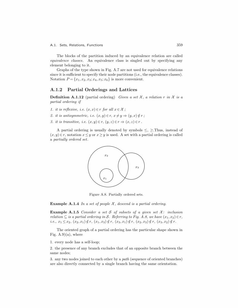
A.1. Sets, Relations, Functions 359
The blocks of the partition induced by an equivalence relation are calledequivalence classes. An equivalence class is singled out by specifying anyelement belonging to it.
Graphs of the type shown in Fig. A.7 are not used for equivalence relationssince it is sufficient to specify their node partitions (i.e., the equivalence classes).Notation P = {x1, x2, x3;x4, x5;x6} is more convenient.
A.1.2 Partial Orderings and Lattices
Definition A.1.12 (partial ordering) Given a set X , a relation r in X is apartial ordering if
1. it is reflexive, i.e. (x, x)∈ r for all x∈X ;
2. it is antisymmetric, i.e. (x, y)∈ r, x �= y ⇒ (y, x) /∈ r ;3. it is transitive, i.e. (x, y)∈ r, (y, z)∈ r ⇒ (x, z)∈ r .
A partial ordering is usually denoted by symbols ≤, ≥.Thus, instead of(x, y)∈ r, notation x≤ y or x≥ y is used. A set with a partial ordering is calleda partially ordered set .
x1
x2
x3
Figure A.8. Partially ordered sets.
Example A.1.4 In a set of people X , descend is a partial ordering.
Example A.1.5 Consider a set S of subsets of a given set X : inclusionrelation ⊆ is a partial ordering in S. Referring to Fig. A.8, we have (x1, x2)∈ r,i.e., x1≤x2, (x2, x1) /∈ r, (x1, x3) /∈ r, (x3, x1) /∈ r, (x2, x3) /∈ r, (x3, x2) /∈ r.
The oriented graph of a partial ordering has the particular shape shown inFig. A.9)(a), where
1. every node has a self-loop;
2. the presence of any branch excludes that of an opposite branch between thesame nodes;
3. any two nodes joined to each other by a path (sequence of oriented branches)are also directly connected by a single branch having the same orientation.

360 Appendix A. Mathematical Background
x1
x1 x2x2
x3
x3
x4
x4
x5
x5
x6
x6
11
1
111
1
1
1
1
0
0
0 0
0
0 000
0 0
0
0
00
0
0
00
000
00
00
(a)
(b)
(c)
Figure A.9. Graph, Hasse diagram, and matrix of a partial ordering.
A partial ordering relation is susceptible to a simpler representationthrough a Hasse diagram, where self-loops and connections implied by otherconnections are not shown and node xi is represented below xj if xi≤xj . TheHasse diagram represented in Fig. A.9(b) corresponds to the graph shown inFig. A.9(a).
The matrix of a partial ordering relation (see Fig. A.9(c)) also has aparticular shape. In fact:
1. rii =1 for all i;
2. rij =1 implies rji =0 for all i, j;
P1
P2 P3 P4
P5
Figure A.10. Hasse diagram of partitions of a set with three elements.

A.1. Sets, Relations, Functions 361
3. rij = rjk =1 implies rik = rij (or rik = rjk) for all i, j, k.
Example A.1.6 Given a set X , in the set of all partition of P1, P2, . . . of Xa partial ordering can be defined by stating that Pi≤Pj if every block of Pi iscontained in a block of Pj . In particular, let X = {x1, x2, x3}: the partitions ofX are P1 = {x1;x2;x3}, P2 = {x1, x2;x3}, P3 = {x1;x2, x3}, P4 = {x1, x3;x2},P5 = {x1, x2, x3},and their Hasse diagram is shown in Fig. A.10.
Definition A.1.13 (lattice) A lattice L is a partially ordered set in which forany pair x, y ∈L there exists a least upper bound (l.u.b.), i.e., an η ∈L suchthat η≥ x, η≥ y and z≥ η for all z ∈L such that z≥ x, z≥ y, and a greatestlower bound (g.l.b.), i.e., an ε∈L such that ε≤x, ε≤ y and z≤ ε for all z ∈Lsuch that z≤ x, z≤ y.
{x1}
{x1, x2}
{x1, x2, x3}
{x2, x3}
{x3}
∅
{x1, x3}
{x2}
Figure A.11. The lattice of all subsets of a set with three elements.
Example A.1.7 The set of all subsets of a given set X , with the partialordering relation induced by inclusion ⊆, is a lattice. Its Hasse diagram inthe case of a set with three elements is shown in Fig. A.11.
Example A.1.8 The set of all partitions P1, P2, . . . of a given set X , with theabove specified partial ordering, is a lattice.
In a lattice, two binary operations, which will be called addition andmultiplication and denoted with symbols + and · , can be defined throughthe relations x+ y= η and x ·y= ε, i.e., as the operations that associate to anypair of elements their g.l.b. and l.u.b. It is easily shown that + and · satisfy
1. idempotency:
x+ x = x ∀x ∈ Lx · x = x ∀x ∈ L

362 Appendix A. Mathematical Background
2. commutative laws:
x+ y = y + x ∀x, y ∈ Lx · y = y · x ∀x, y ∈ L
3. associative laws:
x+ (y + z) = (x + y) + z ∀x, y, z ∈ Lx · (y · z) = (x · y) · z ∀x, y, z ∈ L
4. absorption laws:
x+ (x · y) = x ∀x, y ∈ Lx · (x+ y) = x ∀x, y ∈ L
A lattice is called distributive if distributive laws hold, i.e.
x+ (y · z) = (x+ y) · (x+ z) ∀x, y, z ∈ Lx · (y + z) = (x · y) + (x · z) ∀x, y, z ∈ L
Since + and · are associative, any finite subset of a lattice has a leastupper bound and a greatest lower bound; in particular, any finite lattice has auniversal upper bound or, briefly, a supremum I (the sum of all its elements)and an universal lower bound or, briefly, an infimum O (the product of all itselements), which satisfy
I + x = I , O + x = x ∀x∈LI · x = x , O · x = O ∀x∈L
Also a nonfinite lattice may admit universal bounds. In the case of ExampleA.1.7 the binary operations are union and intersection and the universal boundsare X and ∅. In Example A.1.8 the operations are the sum of partitions,defined as the maximal partition (i.e., the partition with the maximum numberof blocks) whose blocks are unions of blocks of all partitions to be summed,and the product of partitions, defined as the minimal partition whose blocksare intersections of blocks of all partitions to be multiplied; the lattice isnondistributive and the universal bounds are partition PM (with X as theonly block) and Pm (with all elements of X as blocks), called the maximalpartition and the minimal partition respectively.
A.2 Fields, Vector Spaces, Linear Functions
The material presented in this section and in the following one is a selectionof topics of linear algebra in which the most important concepts and theformalism needed in general system theory are particularly stressed: vectorspaces, subspaces, linear transformations, and matrices.
A.2. Fields, Vector Spaces, Linear Functions 363
Definition A.2.1 (field) A field F is a set, whose elements are called scalars,with two binary operations + (addition) and · (multiplication) characterized bythe following properties:
1. commutative laws:
α+ β = β + α ∀α, β ∈ Fα · β = β · α ∀α, β ∈ F
2. associative laws:
α+ (β + γ) = (α+ β) + γ ∀α, β, γ ∈ Fα · (β · γ) = (α · β) · γ ∀α, β, γ ∈ F
3. distributivity of multiplication with respect to addition:
α · (β + γ) = α · β + α · γ ∀α, β, γ ∈ F
4. the existence of a neutral element for addition, i.e., of a unique scalar0∈F (called zero) such that
α+ 0 = α ∀α ∈ F
5. the existence of the opposite of any element: for all α∈F there exists aunique scalar −α∈F such that
α+ (−α) = 0
6. the existence of a neutral element for multiplication, i.e., of a uniquescalar 1∈F (called one) such that
α · 1 = α ∀α ∈ F
7. the existence of the inverse of any element: for all α∈F , α �=0 thereexists a unique scalar α−1 ∈F such that α · α−1 = 1.
Example A.2.1 The set of all real numbers is a field, which is denoted by R.
Example A.2.2 The set of all complex numbers is a field, which is denotedby C.
Example A.2.3 The set B := {0, 1}, with + and · defined as in the tablesshown in Fig. A.12, is also a field, which will be denoted by B.
Definition A.2.2 (vector space) A vector space V over a field F is a set,whose elements are called vectors, with two binary operations + (addition) and· (multiplication by scalars or external product) characterized by the followingproperties:
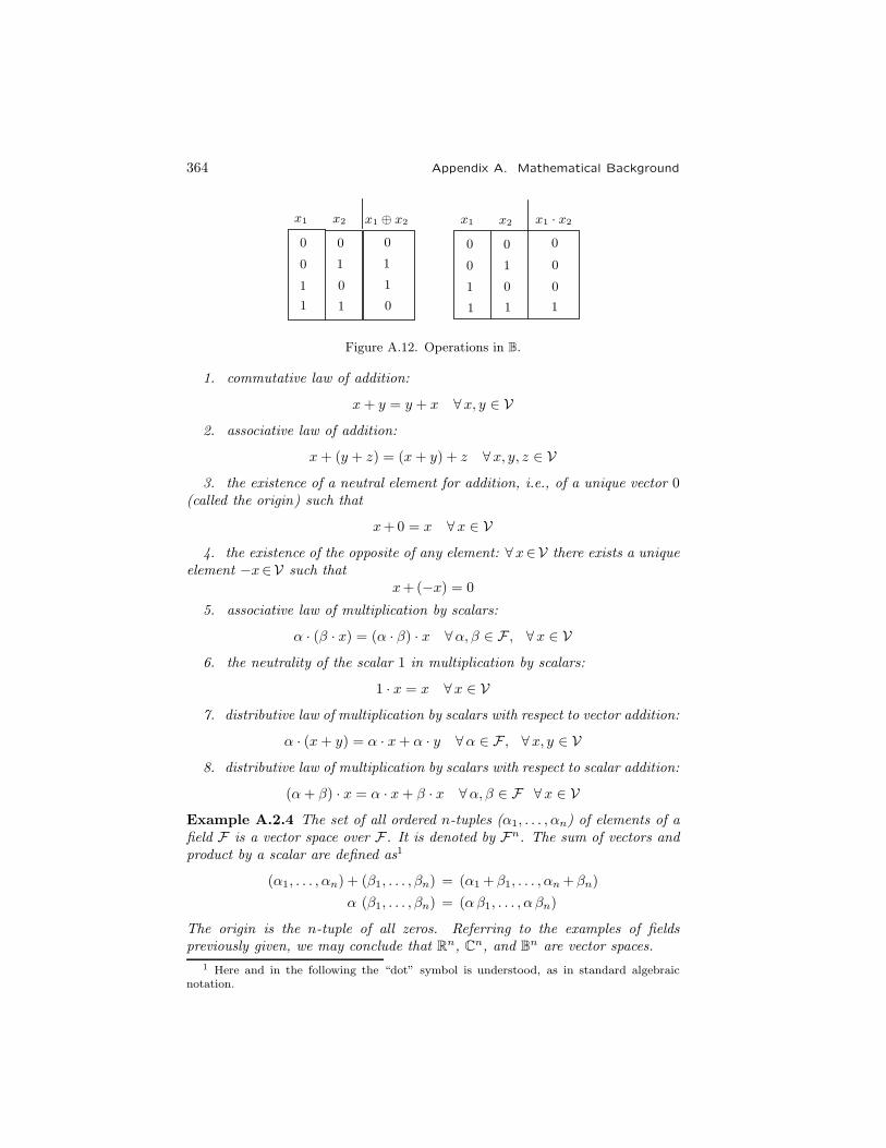
364 Appendix A. Mathematical Background
x1x1 x2x2 x1 ⊕ x2 x1 · x2
1 1 1
1
1
11
11
1
1 0
0
0
0
0
00
0
0
0
0
00
Figure A.12. Operations in B.
1. commutative law of addition:
x+ y = y + x ∀x, y ∈ V
2. associative law of addition:
x+ (y + z) = (x+ y) + z ∀x, y, z ∈ V
3. the existence of a neutral element for addition, i.e., of a unique vector 0(called the origin) such that
x+0 = x ∀x ∈ V
4. the existence of the opposite of any element: ∀x∈V there exists a uniqueelement −x∈V such that
x+(−x) = 0
5. associative law of multiplication by scalars:
α · (β · x) = (α · β) · x ∀α, β ∈ F , ∀x ∈ V
6. the neutrality of the scalar 1 in multiplication by scalars:
1 · x = x ∀x ∈ V
7. distributive law of multiplication by scalars with respect to vector addition:
α · (x+ y) = α · x+ α · y ∀α ∈ F , ∀x, y ∈ V
8. distributive law of multiplication by scalars with respect to scalar addition:
(α+ β) · x = α · x+ β · x ∀α, β ∈ F ∀x ∈ V
Example A.2.4 The set of all ordered n-tuples (α1, . . . , αn) of elements of afield F is a vector space over F . It is denoted by Fn. The sum of vectors andproduct by a scalar are defined as1
(α1, . . . , αn) + (β1, . . . , βn) = (α1 + β1, . . . , αn +βn)
α (β1, . . . , βn) = (αβ1, . . . , α βn)
The origin is the n-tuple of all zeros. Referring to the examples of fieldspreviously given, we may conclude that Rn, Cn, and Bn are vector spaces.
1 Here and in the following the “dot” symbol is understood, as in standard algebraicnotation.

A.2. Fields, Vector Spaces, Linear Functions 365
Example A.2.5 The set of all functions f [t0, t1] or f : [t0, t1] → Fn, piece-wise continuous, i.e., with a finite number of discontinuities in [t0, t1], is avector space over F .
Example A.2.6 The set of all the solutions of the homogeneous differentialequation
d3x
dt3+ 6
d2x
dt2+ 11
dx
dt= 0
which can be expressed as
x(t) = k1 e−t + k2 e
−2t + k3 e−3t (k1, k2, k3) ∈ R
3 (A.2.1)
is a vector space over R.
Example A.2.7 For any positive integer n, the set of all polynomials havingdegree equal or less than n− 1 and coefficients belonging to R, C, or B, is avector space over R, C, or B in which the operations are the usual polynomialaddition and multiplication by a scalar. The origin is the polynomial with allcoefficients equal to zero.
Definition A.2.3 (subspace) Given a vector space V over a field F , a subsetX of V is a subspace of V if
αx+ βy ∈ X ∀α, β ∈ F , ∀x, y ∈ X
Note that any subspace of V is a vector space over F . The origin is asubspace of V that is contained in all other subspaces of V ; it will be denotedby O.
Definition A.2.4 (sum of subspaces) The sum of two subspaces X ,Y ∈V isthe set
X + Y :={z : z = x+ y, x ∈ X , y ∈ Y
}Property A.2.1 The sum of two subspaces of V is a subspace of V.
Proof. Let p, q ∈ X +Y: by definition there exist two pairs of vectorsx, z ∈ X and y, v ∈ Y such that p=x+ y, q= z+ v. Since αp + βq =(αx+ βz) + (αy+ βv) ∀α, β ∈ F , and αx+ βz ∈ X , αy+βv ∈ Y becauseX and Y are subspaces, it follows that αp+ βq ∈ X +Y, hence X +Y is asubspace. �
Definition A.2.5 (intersection of subspaces) The intersection of two sub-spaces X ,Y ∈V is the set
X ∩ Y :={z : z ∈ X , z ∈ Y
}Property A.2.2 The intersection of two subspaces of V is a subspace of V.

366 Appendix A. Mathematical Background
Proof. Let p, q ∈ X ∩Y, i.e., p, q ∈ X and p, q ∈ Y. Since X and Y aresubspaces, αp+βq ∈ X and αp+βq ∈ Y ∀α, β ∈ F . Thus, αp+βq ∈ X ∩Y,hence X ∩Y is a subspace. �
Definition A.2.6 (direct sum of subspaces) Let X ,Y ⊆Z be subspaces of avector space V which satisfy
X + Y = Z (A.2.2)
X ∩ Y = O (A.2.3)
In such a case Z is called the direct sum of X and Y. The direct sum is denotedby the symbol ⊕ ; hence the notation X ⊕Y =Z is equivalent to (A.2.2,A.2.3).
Property A.2.3 Let Z =X ⊕Y. Any vector z ∈Z can be expressed in aunique way as the sum of a vector x∈X and a vector y ∈Y.
Proof. The existence of two vectors x and y such that z= x+ y is a con-sequence of Definition A.2-4. In order to prove uniqueness, assume thatz=x+ y= x1 + y1; by difference we obtain (x− x1)+(y− y1)= 0 or (x− x1) =−(y− y1). Since X ∩Y = O, the only vector belonging to both subspaces isthe origin. Hence (x− x1) = (y− y1)= 0, i.e., x= x1, y= y1. �
Corollary A.2.1 Let Z =X +Y. All decompositions of any vector z ∈Z inthe sum of two vectors belonging respectively to X and Y are obtained fromany one of them, say z= x1 + y1, by summing each vector of X ∩Y to x1 andsubtracting it from y1.
Proof. The proof is contained in that of Property A.2.3. �
Definition A.2.7 (linear variety or manifold) Let x0 be any vector belongingto a vector space V, X any subspace of V. The set2
L ={z : z= x0 +x, x∈X
}= {x0}+ X
is called a linear variety or linear manifold contained in V.
Definition A.2.8 (quotient space) Let X be a subspace of a vector space Vover a field F : the set of all linear varieties
L = {x}+ X , x ∈ V
is called the quotient space of V over X and denoted by V/X .2 Note that the sum of subspaces, as introduced in Definition A.2.4, can be extended to
general subsets of a vector space. Of course, the sum of general subsets in general is not asubspace and does not contain the origin, unless both the addends do.
A.2. Fields, Vector Spaces, Linear Functions 367
A quotient space is a vector space over F . Any two elements of a quotientspace L1 = {x1}+X , L2 = {x2}+X are equal if x1−x2 ∈ X . The sum of L1and L2 is defined as
L1 + L2 := {x1 + x2}+ X
The external product of L = {x}+ X by a scalar α∈F is defined as
αL := {αx}+ X
A.2.1 Bases, Isomorphisms, Linearity
Definition A.2.9 (linearly independent set) A set of vectors {x1, . . . , xh}belonging to a vector space V over a field F is linearly independent if
h∑i=1
αi xi = 0 , αi ∈ F (i=1, . . . , h) (A.2.4)
implies that all αi are zero. If, on the other hand, (A.2.4) holds with some ofthe αi different from zero, the set is linearly dependent.
Note that a set in which at least one of the elements is the origin is linearlydependent. If a set is linearly dependent, at least one of the vectors can beexpressed as a linear combination of the remaining ones. In fact, suppose that(A.2.4) holds with one of the coefficients, for instance α1, different from zero.Hence
x1 = −h∑
i=2
αi
α1xi
Definition A.2.10 (span of a set of vectors) Let {x1, . . . , xh} be any set ofvectors belonging to a vector space V over a field F . The span of {x1, . . . , xh}(denoted by sp{x1, . . . , xh}) is the subspace of X
sp{x1, . . . , xh} :={x : x =
h∑i=1
αi xi , αi ∈ F (i=1, . . . , h)}
Definition A.2.11 (basis) A set of vectors {x1, . . . , xh} belonging to a vec-tor space V over a field F is a basis of V if it is linearly independent andsp{x1, . . . , xh} = V.
Theorem A.2.1 Let (b1, . . . , bn) be a basis of a vector space V over a field F ;for any x∈V there exists a unique n-tuple of scalars (α1, . . . , αn) such that
x =n∑
i=1
αi bi
368 Appendix A. Mathematical Background
Proof. Existence of (α1, . . . , αn) is a consequence of Definition A.2.11, unique-ness is proved by contradiction. Let (α1, . . . , αn), (β1, . . . , βn) be two orderedn-tuples of scalars such that
x =
n∑i=1
αi bi =
n∑i=1
βi bi
Hence, by difference
0 =
n∑i=1
(αi − βi) bi
since the set {b1, . . . , bn} is linearly independent, it follows thatαi =βi (i=1, . . . , n). �
The scalars (α1, . . . , αn) are called the components of x in the basis(b1, . . . , bn).
Example A.2.8 A basis for Fn is the set of vectors
e1 := (1, 0, . . . , 0)e2 := (0, 1, . . . , 0). . . . . . . . .en := (0, 0, . . . , 1)
(A.2.5)
It is called the main basis of Fn. Let x=(x1, . . . , xn) be any element ofFn: the i-th component of x with respect to the main basis is clearly xi.
Example A.2.9 A basis for the vector space (A.2.1), defined in ExampleA.2.6, is
b1 := e−t , b2 := e−2t , b3 := e−3t
Example A.2.10 For the vector space of all piecewise continuous functionsf [t0, t1] it is not possible to define any basis with a finite number of elements.
Theorem A.2.2 The number of elements in any basis of a vector space V isthe same as in any other basis of V.
Proof. Let {b1, . . . , bn} and {c1, . . . , cm} (m≥n) be any two bases of V .Clearly
V = sp{cn, b1, . . . , bn} (A.2.6)
Since cn ∈V it can be expressed as
cn =∑i∈J1
α1i bi , J1 := {1, 2, . . . , n}
At least one of the α1i (i∈J1) is different from zero, cn being different fromthe origin. Let α1j �=0, so that bj can be expressed as a linear combination of

A.2. Fields, Vector Spaces, Linear Functions 369
{cn, b1, . . . , bj− i, bj +1, . . . , bn} and can be deleted on the right of (A.2.6). Byinsertion of the new vector cn− 1 in the set, it follows that
V = sp{cn− 1, cn, b1, . . . , bj− 1, bj +1, . . . , bn} (A.2.7)
Since cn− 1 ∈V and V is the span of the other vectors on the right of (A.2.7),
cn− 1 = β2n cn +∑i∈J2
α2i bi , J2 := {1, . . . , j− 1, j+1, . . . , n}
At least one of the α2i (i∈J2) is different from zero, cn− 1 being different fromthe origin and linearly independent of cn. Again, on the right of (A.2.7) it ispossible to delete one of the bi (i∈J2). By iteration of the same argument, itfollows that
V = sp{c1, . . . , cn}Since set {c1, . . . , cn} is linearly independent, we conclude that it is a basis ofV , hence m=n. �
A vector space V whose bases contain n elements is called an n-dimensionalvector space. The integer n is called the dimension of V , n=dimV in shortnotation. Example A.2.10 above refers to an infinite-dimensional vector space.
Definition A.2.12 (isomorphic vector spaces) Two vector spaces V and Wover the same field F are isomorphic if there exists a one-to-one correspondencet : V →W which preserves all linear combinations, i.e.
t(αx+ βy) = α t(x) + β t(y) ∀α, β ∈ F , ∀x, y ∈ V (A.2.8)
To denote that V and W are isomorphic, notation V ≡W is used.
Function t is called an isomorphism. In order to be isomorphic, V andW must have the same dimension; in fact, by virtue of (A.2.8) a basis in oneof the vector spaces corresponds to a basis in the other. As a consequence ofTheorem A.2.2, any n-dimensional vector space V over F is isomorphic to Fn,hence for any subspace X ⊆V , dimX ≤ dimV .
Corollary A.2.2 Let {b1, . . . , bn} be a basis of a vector space V and{c1, . . . , cm} a basis of a subspace X ∈V. It is possible to extend the set{c1, . . . , cm} to a new basis of V by inserting in it a proper choice of n−mof the elements of the old basis {b1, . . . , bn}.
Proof. The argument developed for the proof of Theorem A.2.2 can beapplied in order to substitute m elements of the basis {b1, . . . , bn} with{c1, . . . , cm}. �
Corollary A.2.3 Let X be a subspace of a vector space V, with dimX =m,dimV =n. The dimension of the quotient space V/X is n−m.

370 Appendix A. Mathematical Background
Proof. Apply Corollary A.2.2: if {b1, . . . , bn} is a basis of V such that{b1, . . . , bm} is a basis of X , the linear varieties
{bi}+ X (i = m+1, . . . , n)
are clearly a basis of V/X . �
Definition A.2.13 (linear function or linear map) A function A : V →W,where V and W are vector spaces over the same field F , is a linear function orlinear map or linear transformation if
A(αx + βy) = αA(x) + β A(y) ∀α, β ∈ F , ∀x, y ∈ V
In other words, a linear function is one that preserves all linear combina-tions. For instance, according to (A.2.8) an isomorphism is a linear function.The particular linear function I : V →V such that I(x) = x for all x∈V iscalled the identity function.
Example A.2.11 Let V be the vector space of all piecewise continuous func-tions x(·) : [t0, t1]→R. The relation
z =
∫ t1
t0
e−(t1−τ) x(τ) dτ
defines a linear function A : V →R.
Definition A.2.14 (image of a linear function) Let A : V →W be a linearfunction. The set
imA :={z : z = A(x), x∈V
}is called the image or range of A. The dimension of imA is called the rank ofA and denoted by ρ(A).
Definition A.2.15 (kernel or null space of a linear function) Let A : V →Wbe a linear function. The set
kerA :={x : x∈V , A(x) = 0
}is called the kernel or null space of A. The dimension of kerA is called thenullity of A and denoted by ν(A).
Property A.2.4 Both imA and kerA are subspaces (of W and V respectively).
Proof. Let z, u∈ imA, so that there exist two vectors x, y ∈V such thatz=A(x), u=A(y). A being linear
α z+β u = αA(x)+ β A(y) = A(αx+β y) ∀α, β ∈ F

A.2. Fields, Vector Spaces, Linear Functions 371
therefore, provided αx+ β y ∈ V , it follows that α z+β u ∈ imA. Letx, y ∈ kerA, so that A(x)=A(y)= 0. Therefore
A(αx+ β y) = αA(x) + β A(y) = 0 ∀α, β ∈ Fhence, αx+ β y ∈ kerA. �
Property A.2.5 Let A : V →W be a linear function and dimV =n. Thefollowing equality holds:
ρ(A) + ν(A) = n
Proof. Let {b1, . . . , bn} be a basis of V and {b1, . . . , bh}, h≤n, a basis of kerA(see Corollary A.2.2). Clearly
sp{A(b1), . . . , A(bn)} = sp{A(bh+1), . . . , A(bn)} = imA
thus, in order to prove the property it is sufficient to show that{A(bh+1), . . . , A(bn)} is a linearly independent set. In fact, the equality
n∑i=h+1
αiA(bi) = A( n∑i=h+1
αi bi
)= 0
i.e.n∑
i=h+1
αi bi ∈ kerA
implies αi=0 (i=h+1, . . . , n), because the last n−h components (with re-spect to the assumed basis) of all vectors belonging to kerA must be zero. �
Property A.2.6 A linear function A : V →W is one-to-one if and only ifkerA = O.
Proof. If. Let kerA=O: for every pair x, y ∈V , x �= y, it follows thatA(x− y) �=0, i.e., A(x) �=A(y).
Only if. By contradiction, suppose kerA �=O and consider a vector x suchthat x ∈ kerA, x �=0. Since A(x)= 0, A(0)=0, A is not one-to-one. �
Property A.2.7 A linear function A : V →W is one-to-one if and only if itmaps linearly independent sets into linearly independent sets.
Proof. If. Let {x1, . . . , xh} be a linearly independent set. Suppose, bycontradiction, that {A(x1), . . . , A(xh)} is linearly dependent, so that there existh scalars α1, . . . , αh not all zero such that α1A(x1)+ . . . +αhA(xh) = 0, henceα1 x1 + . . . +αh xh ∈ kerA. Thus, A is not one-to-one by Property A.2.6.
Only if. Owing to Property A.2.6, kerA �=O if A is not one-to-one; hence,there exists at least one nonzero vector x∈V such that A(x) = 0. Anylinear independent set that includes x is transformed into a set that is linearlydependent because it includes the origin. �

372 Appendix A. Mathematical Background
A.2.2 Projections, Matrices, Similarity
Definition A.2.16 (projection) Let X , Y be any pair of subspaces of a vectorspace V such that X ⊕Y =V. Owing to Property A.2.3, for all z ∈V there existsa unique pair (x, y) such that z=x+ y, x∈X , y∈Y. The linear functionsP : V →X and Q : V →Y defined by
P (z) = x , Q(z) = y ∀ z ∈ V
are called, respectively, the projection on X along Y and the projection on Yalong X .
Note that imP =X , kerP =Y, imQ=Y, kerQ=X .
Definition A.2.17 (canonical projection) Let X be any subspace of a vectorspace V. The linear function P : V →V/X defined by P (x) = {x}+X is calledthe canonical projection of V on V/X .
Note that imP =V/X , kerP =X .Definition A.2.18 (invariant subspace) Let V be a vector space and A :V →V a linear map. A subspace X ⊆V is said to be an invariant under A, oran A-invariant, if
A(X ) ⊆ X
It is easy to prove that the sum and the intersection of two or more A-invariants are A-invariants; hence any subset of the set of all A-invariantscontained in V , closed with respect to sum and intersection, is a lattice withrespect to ⊆,+,∩ .
The following theorem states a very important connection between linearmaps and matrices.
Theorem A.2.3 Let V and W be finite-dimensional vector spaces over thesame field F and {b1, . . . , bn}, {c1, . . . , cm} bases of V and W respectively.Denote by ξi (i=1, . . . , n) and ηi (i=1, . . . ,m) the components of vectors x∈Vand y ∈W with respect to these bases. Any linear function A : V →W can beexpressed as
ηj =n∑
i=1
aji ξi (j = 1, . . . ,m) (A.2.9)
Proof. By definition of linear function, the following equalities hold:
y = A(x) = A( n∑
i=1
ξi bi
)=
n∑i=1
ξiA(bi)
For each value of i, denote by aji (j=1, . . . ,m) the components of A(bi) withrespect to the basis {c1, . . . , cm}, i.e.
A(bi) =
m∑j=1
aji cj

A.2. Fields, Vector Spaces, Linear Functions 373
By substitution, it follows that
y =
n∑i=1
ξi
( m∑j=1
aji cj
)=
m∑j=1
( n∑i=1
aji ξi
)cj
which is clearly equivalent to (A.2.9). �
Relation (A.2.9) can be written in a more compact form as
η = Ax (A.2.10)
where η, A, and ξ are matrices defined as
η :=
⎡⎢⎣η1...ηm
⎤⎥⎦ A :=
⎡⎣ a11 . . . a1n
.... . .
...am1 . . . amn
⎤⎦ ξ :=
⎡⎢⎣ξ1...ξm
⎤⎥⎦
The following corollaries are direct consequences of the argument developedin the proof of Theorem A.2.3.
Corollary A.2.4 Let A : V →W be a linear function represented by the matrixA with respect to the bases {b1, . . . , bn} of V and {c1, . . . , cm} of W. Thecolumns of A are the components of A(b1), . . . , A(bn) in the basis {c1, . . . , cm}.
Corollary A.2.5 Let A : V →V be a linear function represented by the matrixA with respect to the basis {b1, . . . , bn} of V. The columns of A are thecomponents of A(b1), . . . , A(bn) in this basis.
Theorem A.2.3 states that a linear function A : V →W , where V and Ware finite-dimensional vector spaces over the same field F , is given by defininga basis for V , a basis forW , and a matrix with elements in F . The special caseV =Fn, W =Fm may be a source of confusion: in fact, in this case vectorsare m-tuples and n-tuples of scalars, so that apparently only a matrix withelements in F is needed in order to represent a linear function. This does notcontradict Theorem A.2.3, because vectors can be understood to be referredrespectively to the main bases of Fn and Fm so that components coincide withelements of vectors. In this case it is customary to write (A.2.10) directly as
z = Ax (A.2.11)
and call “vectors” the n× 1 and m× 1 matrices representing the n-tuple x andthe m-tuple z, so that (A.2.11) means “vector z is equal to the product ofvector x by matrix A.” For the sake of simplicity, in this case a linear functionand its representing matrix are denoted with the same symbol; hence, notationA : Fn→Fm means “the linear function from Fn into Fm which is representedby the m×n matrix A with respect to the main bases.” Similarly, notationsimA, kerA, ρ(A), ν(A), A-invariant are referred both to functions and matrices.

374 Appendix A. Mathematical Background
Definition A.2.19 (basis matrix) Any subspace X ⊆Fn can be representedby a matrix X whose columns are a basis of X , so that X = imX. Such amatrix is called a basis matrix of X .
Property A.2.8 Let V be an n-dimensional vector space over a field F (F =R
or F =C) and denote by u, v∈Fn the components of any vector x∈V withrespect to the bases {b1, . . . , bn}, {c1, . . . , cn}. These components are related by
u = Tv
where T is the n×n matrix having as columns the components of vectors{c1, . . . , cn} with respect to the basis {b1, . . . , bn}.
Proof. Apply Corollary A.2.5 to the identity function I. �
Since the representation of any vector with respect to any basis is unique,matrix T is invertible, so that
v = T−1u
where T−1, owing to Corollary A.2.5, is the matrix having as columns thecomponents of vectors {b1, . . . , bn} with respect to the basis {c1, . . . , cn}.
Changes of basis are very often used in order to study properties of lineartransformations by analyzing the structures of their representing matrices withrespect to some properly selected bases. Therefore, it is worth knowing howmatrices representing the same linear function with respect to different basesare related to each other.
Property A.2.9 Let A : V →W be a linear function represented by the m×nmatrix A with respect to the bases {b1, . . . , bn}, {c1, . . . , cm}. If new bases{p1, . . . , pn}, {q1, . . . , qm} are assumed for V and W, A is represented by thenew matrix
B = Q−1AP
where P and Q are the n×n and the m×m matrices whose columns are thecomponents of the new bases with respect to the old ones.
Proof. Denote by u, v∈Fn and r, s∈Fm the old and the new componentsof any two vectors x∈V and y ∈W such that y is the image of x in the lineartransformation A: owing to Property A.2.8
u = P v , r = Qs
By substitution into r=Au, we obtain
s = Q−1APv
which directly proves the property. �
In the particular case of a function whose domain and codomain are thesame vector space, we may restate the preceding result as follows.

A.2. Fields, Vector Spaces, Linear Functions 375
Corollary A.2.6 Let A : V →V be a linear function represented by the n×nmatrix A with respect to the basis {b1, . . . , bn}. In the new basis {c1, . . . , cn}function A is represented by the new matrix
B = T−1AT (A.2.12)
where T is the n×n matrix whose columns are the components of the new basiswith respect to the old one.
Let A and B be any two n×n matrices; if there exists a matrix T suchthat equality (A.2.12) holds, A and B are called similar matrices and T asimilarity transformation or an automorphism, i.e., an isomorphism of a vectorspace with itself.
Note that the same similarity transformations relate powers of B and A:in fact, B2 = T−1AT T−1AT = T−1A2T and so on.
Theorem A.2.4 Let X , Y be subspaces of Fn such that X ⊕Y =Fn and X,Y basis matrices of X , Y. Projecting matrices on X along Y and on Y alongX , i.e., matrices that realize the projections introduced as linear functions inDefinition A.2.16, are
P =[X O
] [X Y
]−1(A.2.13)
Q =[O Y
] [X Y
]−1(A.2.14)
Proof. Since the direct sum of X and Y is Fn, matrix [X Y ] is nonsingular;therefore, the image of [X Y ]−1 is Fn, so that imP = X , imQ = Y. SinceP +Q= I, for any z ∈Fn x :=Pz, y :=Qz is the unique pair x∈X , y∈Y suchthat z= x+ y. �
A.2.3 A Brief Survey of Matrix Algebra
In the previous section, matrices were introduced as a means of representinglinear maps between finite-dimensional vector spaces. Operations on linearfunctions, such as addition, multiplication by a scalar, composition, reflect onoperations on the corresponding matrices. In the sequel, we will consider onlyreal matrices and complex matrices , i.e., matrices whose elements are real orcomplex numbers. A matrix having as many rows as columns is called a squarematrix . A matrix having only one row is called a row matrix and a matrixhaving only one column is called a column matrix . The symbol (A)ij denotesthe element of the matrix A belonging to the i-th row and the j-th column and[aij ] the matrix whose general element is aij .
The main operations on matrices are:
1. addition of matrices : given two matrices A and B, both m×n, theirsum C =A+B is the m×n matrix whose elements are the sums of the corre-sponding elements of A and B, i.e., cij = aij + bij (i=1, . . . ,m ; j=1, . . . , n) ;

376 Appendix A. Mathematical Background
2. multiplication of a matrix by a scalar : given a scalar α and an m×nmatrix A, the product P = αA is the m×n matrix whose elements are theproducts by α of the elements of A, i.e., pij =α aij (i=1, . . . ,m ; j=1, . . . , n) ;
3. multiplication of two matrices :3 given an m×n matrix A and a n× pmatrix B, the product C = AB is the m× p matrix whose elements are definedas
cij =
n∑k=1
aik bkj (i=1, . . . ,m ; j=1, . . . , p)
These operations enjoy the following properties:
1. commutative law of addition:4
A+B = B +A
2. associative laws:
(A+B) + C = A+ (B + C)
(αA)B = α (AB)
A (BC) = (AB)C
3. distributive laws:
(α+ β)A = αA+ β A
α (A+B) = αA+ αB
(A+B)C = AC +BC
A (B + C) = AB +AC
A null matrix O is a matrix with all elements equal to zero.An identity matrix I is a square matrix with all elements on the main
diagonal equal to one and all other elements equal to zero. In particular, thesymbol In is used for the n×n identity matrix.
A square matrix A is called idempotent if A2 =A, nilpotent of index q ifAq−1 �=O, Aq =O.
For any real m×n matrix A, the symbol AT denotes the transpose ofA, i.e., the matrix obtained from A by interchanging rows and columns. Itselements are defined by
(AT )ji := (A)ij (i=1, . . . ,m; j=1, . . . , n)
In the complex field, A∗ denotes the conjugate transpose of A, whoseelements are defined by
(A∗)ji := (A)∗ij (i=1, . . . ,m ; j=1, . . . , n)
3 Of course, the same rules hold for the product c=Ab, where the “vectors” b and c aresimply n× 1 and m× 1 column matrices.
4 It is worth noting that in general the multiplication of matrices is not commutative, i.e.,in general AB =BA. Hence, instead of saying “multiply A by B,” it is necessary to state“multiply A by B on the left (right)” or “premultiply (postmultiply) A by B.”
A.2. Fields, Vector Spaces, Linear Functions 377
A real matrix A such that AT =A is called symmetric, while a complexmatrix A such that A∗=A is called hermitian.
A square matrix A is said to be invertible if it represents an invertible linearfunction; in such a case A−1 denotes the inverse matrix of A. If A is invertible,the relations C =AB and B=A−1 C are equivalent. An invertible matrix andits inverse matrix commute, i.e., A−1A=AA−1 = I.
In the real field the transpose and the inverse matrices satisfy the followingrelations:
(AT )T = A (A.2.15)
(A+B)T = AT +BT (A.2.16)
(AB)T = BTAT (A.2.17)
(A−1)−1 = A (A.2.18)
(AB)−1 = B−1A−1 (A.2.19)
(A−1)T = (AT )−1 (A.2.20)
Note that (A.2.17) implies that for any A the matrices AAT and ATA aresymmetric. In the complex field, relations (A.2.15−−A.2.17,A.2.20) hold forconjugate transpose instead of transpose matrices.
The trace of a square matrix A, denoted by trA, is the sum of all theelements on the main diagonal, i.e.
trA :=
n∑i=1
aii (A.2.21)
Let A be a 2× 2 matrix: the determinant of A, denoted by detA, is definedas
detA := a11a22 − a12a21If A is an n×n matrix, its determinant is defined by any one of the recursionrelations
detA :=n∑
i=1
aij Aij (j = 1, . . . , n)
= =
n∑j=1
aij Aij (i = 1, . . . , n) (A.2.22)
where Aij denotes the cofactor of aij , which is defined as (−1)i+j times thedeterminant of the (n− 1)× (n− 1) matrix obtained by deleting the i-th rowand the j-th column of A.
The transpose (or conjugate transpose) of the matrix of cofactors [Aij ]T
(or [Aij ]∗) is called the adjoint matrix of A and denoted by adjA.
Any square matrix A such that detA=0 is called singular ; in the oppositecase it is called nonsingular .
The main properties of determinants are:

378 Appendix A. Mathematical Background
1. in the real field, detA = detAT ; in the complex field, detA = detA∗;
2. let B be a matrix obtained from A by interchanging any two rows orcolumns: detB = −detA ;
3. if any two rows or columns of A are equal, detA = 0 ;
4. let B be a matrix obtained from A by adding one row or column multipliedby a scalar α to another row or column: detB = detA ;
5. if any row or column of A is a linear combination of other rows or columns,detA = 0 ;
6. let A, B be square matrices having equal dimensions: det(AB) =detAdetB .
Theorem A.2.5 Let A be a nonsingular matrix. Its inverse matrix A−1 isgiven by
A−1 =adjA
detA(A.2.23)
Proof. Denote by B the matrix on the right of (A.2.23): owing to property 3of the determinants
n∑k=1
aik Ajk =
{detA if i= j0 if i �= j
Then, for any element of the matrix P :=AB
pij =1
detA
n∑k=1
aik Ajk =
{1 if i= j0 if i �= j
Hence, P = I, so that B=A−1. �As a consequence of Theorem A.2.5, we may conclude that a square matrix
is invertible if and only if it is nonsingular.
Partitioned Matrices. A partitioned matrix is one whose elements arematrices, called submatrices of the original nonpartitioned matrix. It is easilyseen that, if partitioning is congruent, addition and multiplication can beperformed by considering each of the submatrices as a single element. Toshow how partitioning is used, let us consider some examples:
[ n1 n2
m1 A Bm2 C D
]+
[ n1 n2
m1 E Fm2 G H
]=
[ n1 n2
m1 A+ E B + Fm2 C +G D +H
]
[ n1 n2
m1 A Bm2 C D
]·
[ p1 p2
n1 E Fn2 G H
]=
[ p1 p2
m1 AE +BG AF +BHm2 CE +DG CF +DH
]

A.3. Inner Product, Orthogonality 379
[ n1 n2
m1 A Bm2 C D
]·
[ p
n1 En2 F
]=
[ p
m1 AE +BFm2 CE +DF
]
Consider a square matrix partitioned into four submatrices as follows:
A =
[B CD E
](A.2.24)
and assume that B and E are square matrices. It is easy to prove by inductionthat if one of the off-diagonal matrices C and D is null, the following holds:
detA = detB detE (A.2.25)
If detB is different from zero, so that B is invertible, by subtracting fromthe second row of (A.2.24 ) the first multiplied on the left by DB−1, we obtainthe matrix [
B CO E −DB−1C
]whose determinant is equal to detA owing to the preceding property 4 of thedeterminants, so that
detA = detB det(E−DB−1C) (A.2.26)
Similarly, if detE �=0, by subtracting from the first row of (A.2.24) the secondmultiplied on the left by CE−1, we obtain
detA = detE det(B−CE−1D) (A.2.27)
A.3 Inner Product, Orthogonality
Providing a vector space with an inner product is a source of some substan-tial advantages, particularly when the maximum universality and abstractnessof approach is not called for. The most significant of these advantages are:a deeper insight into the geometric meaning of many conditions and proper-ties, a straightforward way to consider and possibly avoid ill-conditioning incomputations, a valid foundation for setting duality arguments (depending onproperties of adjoint transformations, hence on the introduction of an innerproduct).
Definition A.3.1 (inner Product) Let V be a vector space defined over thefield R of real numbers. An inner product or scalar product is a function〈· , ·〉 : V ×V →F that satisfies
1. commutativity:〈x, y〉 = 〈y, x〉 ∀x, y ∈ V

380 Appendix A. Mathematical Background
2. linearity with respect to a left-hand factor:
〈αx+ βy , z〉 = α 〈x, z〉+ β 〈y, z〉 ∀α, β ∈ R, ∀x, y, z ∈ V
3. positiveness:
〈x, x〉 ≥ 0 ∀x ∈ V〈x, x〉 = 0 ⇔ x = 0
If V is defined over the field C of the complex numbers, the preceding property3 still holds, while 1 and 2 are replaced respectively by
1. conjugate commutativity:
〈x, y〉 = 〈y, x〉∗ ∀x, y ∈ V
2. conjugate linearity with respect to a left-hand factor:
〈αx+ βy , z〉 = α∗〈x, z〉+ β∗〈y, z〉 ∀α, β ∈ C , ∀x, y, z ∈ V
A vector space with an inner product is called an inner product space.Note that in the real field, commutativity and linearity with respect to
a left-hand factor imply linearity with respect to a right-hand one, hencebilinearity, while in the complex field conjugate commutativity and conjugatelinearity with respect to a left-hand factor imply linearity with respect to aright-hand factor. In fact:
〈x , αy+βz〉 = 〈αy+ βz , x〉∗
= (α∗〈y, x〉+ β∗〈z, x〉)∗
= α〈x, y〉 + β〈x, z〉
Example A.3.1 In Rn an inner product is
〈x, y〉 :=n∑
i=1
xiyi (A.3.1)
and in Cn
〈x, y〉 :=n∑
i=1
x∗i yi (A.3.2)
Note that in Rn and Cn, vectors can be considered as n× 1 matrices, sothat the notations xT y and x∗y may be used instead of 〈x, y〉.
Example A.3.2 In any finite-dimensional vector space over R or C an innerproduct is defined as in (A.3.1) or (A.3.2), where (x1, . . . , xn) and (y1, . . . , yn)denote components of vectors with respect to given bases.

A.3. Inner Product, Orthogonality 381
Example A.3.3 In the vector space of all piecewise continuous time functionsf(·) : [t0, t1]→ Fn (with F = R or F = C) an inner product is
〈x, y〉 :=∫ t1
t0
〈x(t) y(t)〉 dt
Definition A.3.2 (euclidean morm) Let V be an inner product space and xany vector belonging to V. The real nonnegative number
‖x‖ :=√〈x, x〉 (A.3.3)
is called the euclidean norm of x.
The euclidean norm is a measure of the “length” of x, i.e., of the distanceof x from the origin.
Definition A.3.3 (orthogonal vectors) A pair of vectors x, y belonging to aninner product space are said to be orthogonal if 〈x, y〉 = 0.
Definition A.3.4 (orthonormal set of vectors) A set of vectors {u1, . . . , un}belonging to an inner product space is orthonormal if
〈ui, uj〉 = 0 (i = 1, . . . , n ; j = 1, . . . , i− 1, i+1, . . . , n)
〈ui, ui〉 = 1 (i = 1, . . . , n)
Fromn∑
i=1
αiui = 0
through the left inner product of both members by u1, . . . , un, we obtainα1 =0, . . . , αn =0, so we may conclude that an orthonormal set is a linearlyindependent set.
Definition A.3.5 (orthogonal matrix and unitary matrix) An n×n real ma-trix is orthogonal if its rows (columns) are orthonormal sets. In the complexfield, such a matrix is called unitary.
It is easy to check that a necessary and sufficient condition for a squarematrix U to be orthogonal (unitary) is
UTU = U UT = I (U∗U = U U∗ = I )
Therefore, the inverse of an orthogonal (unitary) matrix can be determined bysimply interchanging rows and columns.
Orthogonal (unitary) matrices have the interesting feature of preservingorthogonality of vectors and values of inner products. The product of two ormore orthogonal (unitary) matrices is an orthogonal (unitary) matrix. In fact,if A,B are orthogonal:
(AB)T (AB) = BT (ATA)B = BTB = I
Similar manipulations can be set for unitary matrices.

382 Appendix A. Mathematical Background
Property A.3.1 Let V be a finite-dimensional inner product space. The com-ponents (ξ1, . . . , ξn) of any vector x∈V with respect to an orthonormal basis(u1, . . . , un) are provided by
ξi = 〈ui, x〉 (i = 1, . . . , n) (A.3.4)
Proof. Consider the relation
x =
n∑i=1
ξiui
and take the left inner product of both members by the orthonormal set(u1, . . . , un). �
It is possible to derive an orthonormal basis for any finite-dimensional vec-tor space or subspace through the Gram-Schmidt orthonormalization process(see Algorithm B.2.1).
Definition A.3.6 (adjoint of a linear map) A linear map B is called adjointto a linear map A if for any two vectors x, y belonging respectively to thedomains of A and B the following identity holds:
〈Ax, y〉 = 〈x,By〉
Property A.3.2 Let A be an m×n real matrix. The inner product (A.3.1)satisfies the identity
〈Ax, y〉 = 〈x,AT y〉 ∀x ∈ Rn, ∀ y ∈ R
m (A.3.5)
while, if A is complex and the inner product is defined as in (A.3.2)
〈Ax, y〉 = 〈x,A∗y〉 ∀x ∈ Cn, ∀ y ∈ C
m (A.3.6)
Proof. Equalities (A.3.5,A.3.6) follow from matrix identity (Ax)T y = xTAT y,which is a consequence of (A.2.17), and (Ax)∗y = x∗A∗y. �
It follows that if a linear map is represented by a real (a complex) matrixwith respect to an orthonormal basis, its adjoint map is represented by thetranspose (the conjugate transpose) matrix with respect to the same basis.
Definition A.3.7 (orthogonal complement of a subspace Let V be an innerproduct space and X any subspace of V. The set
X⊥ ={y : 〈x, y〉 = 0, x ∈ X
}(A.3.7)
is called the orthogonal complement of X .
It is easily seen that X⊥ is a subspace of V .
A.3. Inner Product, Orthogonality 383
Property A.3.3 Let V be an inner product space and X any finite-dimensional subspace of V.5 Then
V = X ⊕ X⊥
Proof. First note that X ∩X⊥= {0} because 〈x, x〉=0 implies x=0. Let{u1, . . . , uh} be an orthonormal basis of X . For any z ∈V consider the decom-position z=x+ y defined by
x =
h∑i=1
ξiui , ξi = 〈ui, z〉
y = z − x = z −h∑
i=1
ξiui
Clearly, x∈X . Since 〈ui, y〉=0 (i=1, . . . , h), y ∈X⊥. �
All statements reported hereafter in this section will refer to real matri-ces; their extension to complex matrices simply requires the substitution oftranspose matrices with conjugate transpose.
Property A.3.4 For any real matrix A
kerAT = (imA)⊥ (A.3.8)
Proof. Let y ∈ (imA)⊥, so that 〈y,AAT y〉 = 0 (in fact clearly AAT y∈ imA),i.e. 〈AT y,AT y〉 = 0, hence AT y=0, y ∈ kerAT . On the other hand, ify ∈ kerAT , 〈AT y, x〉 = 0 for all x, i.e. 〈y,Ax〉 = 0, hence y ∈ (imA)⊥. �
Property A.3.5 For any real matrix A
ρ(A) = ρ(AT ) (A.3.9)
Proof. Let A be m×n : owing to Properties A.3.3 and A.3.4, it is pos-sible to derive a basis of Rm whose elements belong to kerAT and (imA)⊥:it follows that ν(AT )+ ρ(A)=m ; on the other hand, from Property A.2.5,ρ(AT )+ ν(AT )=m. �
Hence, if A is not a square matrix, ν(A) �= ν(AT ).
Property A.3.6 For any real matrix A
imA = im(AAT )
Proof. Let A be m×n ; take a basis of Rn whose elements are in part a basisof imAT and in part a basis of kerA. The vectors of this basis transformedby A span imA by definition. Since vectors in kerA are transformed into theorigin, it follows that a basis of imAT is transformed into a basis of imA. �
5 The finiteness of the dimensions of X is a more restrictive than necessary assumption:Property A.3.3 applies also in the more general case where X is any subspace of an infinite-dimensional Hilbert space.
384 Appendix A. Mathematical Background
A.3.1 Orthogonal Projections, Pseudoinverse of a LinearMap
Definition A.3.8 (orthogonal projection) Let V be a finite-dimensional innerproduct space and X any subspace of V. The orthogonal projection on X is theprojection on X along X⊥.
Corollary A.3.1 Let X be any subspace of Rn (Cn) and U an orthonormal(unitary) basis matrix of X . The orthogonal projection matrices on X and X⊥are
P = U UT (P = U U∗) (A.3.10)
Q = I − U UT (Q = I − U U∗) (A.3.11)
Proof. The proof is contained in that of Property A.3.3. �
Lemma A.3.1 Let V be an inner product vector space and x, y ∈V orthogonalvectors. Then
‖x+ y‖2 = ‖x‖2 + ‖y‖2
Proof.
‖x+ y‖2 = 〈(x+ y), (x+ y)〉= 〈x, x〉+ 〈x, y〉+ 〈y, x〉 + 〈y, y〉= 〈x, x〉+ 〈y, y〉 = ‖x‖2 + ‖y‖2 �
Theorem A.3.1 Let X be any subspace of an inner product space V and Pthe orthogonal projection on X . Then
‖x− P x‖ ≤ ‖x− y‖ ∀x ∈ V , ∀ y ∈ X
Proof. Since (x−Px)∈X⊥, (Px− y)∈X , from Lemma A.3.1 it follows that
‖x− y‖2 = ‖x− P x+ P x− y‖2 = ‖x− P x‖2 + ‖P x− y‖2 �
Theorem A.3.1 is called the orthogonal projection theorem and states thatin an inner product space the orthogonal projection of any vector on a subspaceis the vector of this subspace whose distance (in the sense of euclidean norm)from the projected vector is minimal.
Theorem A.3.2 Let X be any subspace of Rn and X a basis matrix of X .Orthogonal projection matrices on X and X⊥ are:
P = X(XTX)−1XT (A.3.12)
Q = I −X(XTX)−1XT (A.3.13)

A.3. Inner Product, Orthogonality 385
Proof. Let h := dimX ; note that the n×n matrix XTX is nonsingular sinceρ(XTX)= ρ(XT ) owing to Property A.3.6 and ρ(XT )= ρ(X)=h by PropertyA.3.5. Any x∈X can be expressed as x=Xa, a∈Rh, so it is easily checkedthat Px=x. On the other hand, any y ∈X⊥, so that XTy=0, clearly satisfiesPy=0. �
Note that (A.3.10,A.3.11) perform the same operations as (A.3.12,A.3.13);however, in the latter case the basis referred to has not been assumed to beorthonormal.
Theorem A.3.2 suggests an interesting analysis in geometric terms of someintrinsic properties of linear maps. Consider a linear function A : Rn→Rm: asan example, consider the particular case reported in Fig. A.13, wherem=n=3,ρ(A)= 2.
Rn
kerA kerAT
Rm
y w
A+
A
z s
A−11A1
x=A+ z=A+ r
r=Aw=Ax
imAT
imA
Figure A.13. Characteristic subspaces of a linear map.
Any vector w∈Rn can be expressed as w=x+ y, x∈ imAT , y∈ kerA, sothat Aw=A(x+ y)=Ax= r. Hence, the linear function A can be considered asthe composition of the orthogonal projection on imAT and the linear functionA1 : imAT → imA defined as A1(x)=A(x) for all x∈ imAT , which is invertiblebecause any basis of imAT is transformed by A into a basis of imA (PropertyA.3.6).
In order to extend the concept of invertibility of a linear map it is possibleto introduce its pseudoinverse A+ : Rm→Rn which works in a similar way: toany vector z ∈Rm it associates the unique vector x∈ imAT which correspondsin A−11 to the orthogonal projection r of z on imA. Note that A+ is uniqueand that (A+)+ = A.
Theorem A.3.3 Let A be any m×n real matrix. The pseudoinverse of A is
A+ = ATX(XTAATX)−1XT (A.3.14)
where X denotes an arbitrary basis matrix of imA.
Proof. From Property A.3.6 it follows that ATX is a basis matrix of imAT ,so that according to (A.3.12), ATX(XTAATX)−1XTA is the matrix that

386 Appendix A. Mathematical Background
performs the orthogonal projection from Rn on imAT . The correspondinglinear map can be considered as the composition of A : Rn→ imA and A−11 :imA→ imAT , the inverse of one-to-one map A1 previously defined. Matrix(A.3.14) represents A−11 with respect to the main bases of Rn and Rm. In fact,let h := ρ(A)= ρ(AT ); ATXa, a∈Rh, is a generic vector belonging to imAT ,and AATXa is its image in A or in A1. By direct substitution
A+AATX a = ATX(XTAATX)−1XTAATX a = ATX a
Hence, (A.3.14) expresses A−11 when applied to vectors belonging to imA.Furthermore, it maps vectors of kerAT into the origin, being XTx=0 for allx∈ kerAT . �
It is worth investigating the meaning of the pseudoinverse in connectionwith the matrix linear equation
Ax = b (A.3.15)
If (A.3.15) admits at least one solution in x, i.e., if b∈ imA, x :=A+b is thesolution with the least euclidean norm, i.e., the only solution belonging toimAT . The set of all solutions is the linear variety
X := {A+b}+ kerA (A.3.16)
If, on the other hand, b /∈ imA, equation (A.3.15) has no solution; in thiscase the pseudosolution x :=A+b is the vector having the least euclidean normtransformed by A into a vector whose distance from b is a minimum.
When matrix A has maximum rank, i.e., when its rows or columns are alinearly independent set, the expression of A+ can be simplified, as stated inthe following corollary.
Corollary A.3.2 Let A be an m×n real matrix. If m≤n, ρ(A)=m, thepseudoinverse of A is
A+ := AT (AAT )−1 (A.3.17)
If, on the other hand, m≥n, ρ(A)=n, the pseudoinverse of A is
A+ := (ATA)−1AT (A.3.18)
Proof. Referring first to (A.3.18), note that AT (AAT )−1A is the orthogonalprojection matrix from Rn onto imAT . Since in this case imA = Rm, thereexists for any z at least one w such that z = Aw, then AT (AAT )−1z is theorthogonal projection of w on imAT . In order to prove (A.3.18), note thatA(ATA)−1AT is the orthogonal projection matrix from Rm onto imA. Sincein this case kerA= {0}, for any z note that w := (ATA)−1AT z is the uniquevector such that Aw coincides with the orthogonal projection of z on imA. �
When the pseudoinverse of A can be defined as in (A.3.17), its product onthe left by A is clearly the m×m identity matrix, i.e., AA+ = Im, while in the

A.4. Eigenvalues, Eigenvectors 387
case where (A.3.18) holds, the product on the right of the pseudoinverse by Ais the n×n identity matrix, i.e., A+A = In. Hence (A.3.17) and (A.3.18) arecalled the right inverse and the left inverse of matrix A and, in these cases, Ais said respectively to be right-invertible and left-invertible.
Note that relation (A.3.18) embodies the least squares method of linearregression, whose geometrical meaning is clarified by the projection theorem;hence, the general pseudoinverse can be advantageously used when a leastsquares problem admits of more than one solution.
A.4 Eigenvalues, Eigenvectors
Eigenvalues and eigenvectors represent a useful summary of information aboutthe features of linear transformations and are the basic instruments for derivingsimplified (canonical) forms of general matrices through similarity transforma-tions. The most important of these forms, the Jordan canonical form, is a pow-erful means for investigating and classifying linear systems according to theirstructure. Furthermore, eigenvalues are the protagonists of the paramountproblem of control theory, i.e., stability analysis of linear time-invariant sys-tems.
Given any real or complex n×n matrix A, consider, in the complex field,the equation
Ax = λx
which can also be written
(λI −A)x = 0 (A.4.1)
This equation admits nonzero solutions in x if and only if (λI −A) is singular,i.e.,
det(λI −A) = 0 (A.4.2)
The left side of equation (A.4.2) is a polynomial p(λ) of degree n in λ,which is called the characteristic polynomial of A: it has real coefficients if Ais real. Equation (A.4.2) is called the characteristic equation of A and admitsn roots λ1, . . . , λn, in general complex, which are called the eigenvalues orcharacteristic values of A. If A is real, complex eigenvalues are conjugate inpairs. The set of all eigenvalues of A is called the spectrum of A.
To each eigenvalue λi (i=1, . . . , n) there corresponds at least one nonzeroreal or complex vector xi which satisfies equation (A.4.1); this is called aneigenvector or characteristic vector of A. Since for any eigenvector xi, αxi,α∈R, is also an eigenvector, it is convenient to use normalized eigenvectors,i.e., eigenvectors with unitary euclidean norm.
Note that, if A is real:
1. the eigenvectors corresponding to complex eigenvalues are complex: infact Ax = λx cannot be satisfied for λ complex and x real;

388 Appendix A. Mathematical Background
2. if λ, x are a complex eigenvalue and a corresponding eigenvector, x∗ isan eigenvector corresponding to λ∗: in fact, Ax∗ is the conjugate of Ax, λ∗x∗
the conjugate of λx.
Theorem A.4.1 Let A be an n×n real or complex matrix. If the eigenvaluesof A are distinct, the corresponding eigenvectors are a linearly independent set.
Proof. Assume, by contradiction, that eigenvectors x1, . . . , xh, h<n, arelinearly independent, while xh+1, . . . , xn are linearly dependent on them, sothat
xj =
n∑i=1
αijxj (j = h+1, . . . , n)
Since xi is an eigenvector, it follows that
Axj = λjxj =
h∑i=1
αijxi ( j = h+1, . . . , n)
Axj = A
( h∑i=1
αijxi
)=
h∑i=1
αij Axi
=
h∑i=1
αijλixi ( j = h+1, . . . , n)
By difference, we obtain in the end
0 =
n∑i=1
αij(λj − λi)xi ( j = h+1, . . . , n)
Since the scalars αij cannot all be zero and the set {x1, . . . , xh} is linearlyindependent, it follows that λi =λj for at least one pair of indexes i, j. �
Similarity transformations of matrices were introduced in Subsection A.2.2.A fundamental property of similar matrices is the following.
Property A.4.1 Similar matrices have the same eigenvalues.
Proof. Let A, B be similar, so that B = T−1AT . Hence
det(λI − T−1AT ) = det(λT−1I T − T−1AT )= det
(T−1(λI −A)T
)= detT−1 det(λI −A) detT
Since detT−1 and detT are different from zero, any λ such that det(λI −A)= 0also satisfies det(λI −B)= 0. �
Any n×n real or complex matrix A is called diagonalizable if it is similarto a diagonal matrix Λ, i.e., if there exists a similarity transformation T suchthat Λ = T−1AT . In such a case, Λ is called the diagonal form of A.

A.4. Eigenvalues, Eigenvectors 389
Theorem A.4.2 An n×n real or complex matrix A is diagonalizable if andonly if it admits a linearly independent set of n eigenvectors.
Proof. If. Let {t1, . . . , tn} be a linearly independent set of eigenvectors, sothat
Ati = λi ti (i = 1, . . . , n) (A.4.3)
Note that in (A.4.3) λ1, . . . , λn are not necessarily distinct. Equation (A.4.3)can be compacted as
AT = T Λ (A.4.4)
where T is nonsingular and Λ is diagonal.Only if. If A is diagonalizable, there exists a diagonal matrix Λ and a
nonsingular matrix T such that (A.4.4) and, consequently, (A.4.3) hold. Hence,the columns of T must be eigenvectors of A. �
Note that owing to Theorem A.4.2 any square matrix A whose eigenvaluesare distinct admits a diagonal form in which the elements on the main diagonalare the eigenvalues of A. On the other hand, if A has multiple eigenvalues, itis still diagonalizable only if every multiple eigenvalue corresponds to as manylinearly independent eigenvectors as its degree of multiplicity.
In general, the diagonal form is complex also when A is real; this is a diffi-culty in computations, so that it may be preferable, when A is diagonalizable,to derive a real matrix, similar to A, having a 2× 2 submatrix on the maindiagonal for each pair of conjugate complex eigenvalues. The correspondingsimilarity transformation is a consequence of the following lemma.
Lemma A.4.1 Let {u1 + jv1, . . . , uh+ jvh, u1− jv1, . . . , uh− jvh} be a lin-early independent set in the complex field. Then the set {u1, . . . , uh, v1, . . . , vh}is linearly independent in the real field.
Proof. Consider the identity
h∑i=1
(αi + jβi)(ui + jvi) +
h∑i=1
(γi+ jδi)(ui− jvi)
=
h∑i=1
((αi + γi)ui + (δi− βi)vi
)+
j
h∑i=1
((δi +βi)ui + (αi− γi)vi
)(A.4.5)
By contradiction: since, for each value of i, (αi + γi), (αi− γi), (δi +βi),(δi− βi) are four arbitrary numbers, if set {u1, . . . , uh} is linearly dependent itis possible to null the linear combination (A.4.5) with coefficients αi, βi, γi, δi(i=1, . . . , n) not all zero. �

390 Appendix A. Mathematical Background
Theorem A.4.3 Let A be a diagonalizable real matrix, λi (i= i, . . . , h) itsreal eigenvalues, σi + jωi, σi− jωi (i=1, . . . , k), k = (n− h)/2, its complexeigenvalues. There exists a similarity transformation T such that
B = T−1AT
=
⎡⎢⎢⎢⎢⎢⎢⎢⎢⎢⎢⎢⎢⎢⎣
λ1 0 . . . 0 0 0 . . . 0 00 λ2 . . . 0 0 0 . . . 0 0...
.... . .
......
.... . .
......
0 0 . . . λh 0 0 . . . 0 00 0 . . . 0 σ1 ω1 . . . 0 00 0 . . . 0 −ω1 σ1 . . . 0 0...
.... . .
......
.... . .
......
0 0 . . . 0 0 0 . . . σk ωk
0 0 . . . 0 0 0 . . . −ωk σk
⎤⎥⎥⎥⎥⎥⎥⎥⎥⎥⎥⎥⎥⎥⎦
(A.4.6)
Proof. Since A is diagonalizable, it admits a set of n linearly independenteigenvectors: let T be the matrix whose columns are the real eigenvectorsand the real and imaginary part of each pair of complex eigenvectors. For ageneral pair of conjugate complex eigenvalues σ± jω and the correspondingeigenvectors u± jv, relation (A.4.1) becomes
Au± jAv = σu − ωv ± j(σv + ωu)
or, by splitting the real and imaginary parts
Au = σu− ωvAv = ωu+ σv
which imply for B the structure shown in (A.4.6), since u and v are columnsof the transformation matrix T . �
Unfortunately, not all square matrices are diagonalizable, so that we arefaced with the problem of defining a canonical form6 which is as close as possibleto the diagonal form and similar to any n×n matrix. This is the Jordan form,of paramount importance for getting a deep insight into the structure of lineartransformations. On the other hand, unfortunately the Jordan form turns outto be rather critical from the computational standpoint, since the transformedmatrix may be ill-conditioned and very sensitive to small parameter variationsand rounding errors.
6 In a given class of matrices (e.g., general real or complex matrices, or square matricesor idempotent matrices) a canonical form is one that induces a partition under the propertyof similarity, in the sense that in every subclass only one matrix is in canonical form.

A.4. Eigenvalues, Eigenvectors 391
A.4.1 The Schur Decomposition
A much less critical similarity transformation, which can be used for any realor complex square matrix, is considered in the following theorem.
Theorem A.4.4 (the Schur decomposition) Let A be any real or complexn×n matrix. There exists a unitary similarity transformation U that takes Ainto the upper-triangular form
B = U∗AU =
⎡⎢⎢⎣λ1 b12 . . . b1n0 λ2 . . . b2n...
.... . .
...0 0 . . . λn
⎤⎥⎥⎦ (A.4.7)
Proof. The argument is by induction. First assume n=2 and denote by λ1and λ2 the eigenvalues of A; by u1 a normalized eigenvector corresponding toλ1; by u2 any vector orthogonal to u1 with unitary euclidean norm. Define Was the 2× 2 matrix having u1, u2 as columns so that, provided Au1 =λ1 u1
W ∗AW =
[〈u1, A u1〉 〈u1, A u2〉〈u2, A u1〉 〈u2, A u2〉
]
=
[λ1 b120 b22
]=
[λ1 b120 λ2
]
where the last equality is a consequence of Property A.4.1.Assume that the theorem is true for (n− 1)× (n− 1) matrices. Let λ1 be
an eigenvalue of A, u1 a corresponding normalized eigenvector, and u2, . . . , unany orthonormal set orthogonal to u1. By a procedure similar to the previousone, it is proved that the unitary matrix W whose columns are u1, . . . , un issuch that
W ∗AW =
⎡⎢⎢⎣λ1 b12 . . . b1n0 b22 . . . b2n...
.... . .
...0 bn2 . . . bnn
⎤⎥⎥⎦ =
[λ1 b0O B1
]
where b0 denotes a 1× (n− 1) matrix and B1 an (n− 1)× (n− 1) matrix. Bythe induction hypothesis, there exists an (n− 1)× (n− 1) unitary matrix U1
such that U∗1B1U1 is an upper-triangular matrix. Let
V :=
[1 OO U1
]
It follows that
V ∗(W ∗AW )V =
[1 OO U∗1
] [λ1 b0O B1
] [1 OO U1
]
=
[λ1 bO U∗1B1U1
]�

392 Appendix A. Mathematical Background
A.4.2 The Jordan Canonical Form. Part I
An important role in deriving the Jordan canonical form is played by theproperties of nilpotent linear maps.
Lemma A.4.2 A linear map A : Fn→Fn is nilpotent of index q≤n if andonly if all its eigenvalues are zero.
Proof. Only if. Let A be nilpotent of order q. Assume that λ is anonzero eigenvalue, x a corresponding eigenvector. From Ax=λx, it fol-lows that A2x=λAx, . . . , Aqx=λAq− 1x. Since λ is nonzero, Aqx=0 impliesAq− 1x=Aq− 2x= . . . =Ax=0, hence x=0, which contradicts the assump-tion that x is an eigenvector.
If. Let B be an upper-triangular form of A. If all the eigenvalues of Aare zero, the main diagonal of B is zero. It is easily seen that in B2, B3, . . .successive diagonals above the main diagonal vanish, so that at most Bn, andconsequently An, is a null matrix. �
Theorem A.4.5 Let A : Fn→Fn be a linear map nilpotent of index q. Thereexists a similarity transformation T that takes A into the canonical form:
B = T−1AT =
⎡⎢⎢⎣B1 O . . . OO B2 . . . O...
.... . .
...O O . . . Br
⎤⎥⎥⎦ (A.4.8)
where the Bi (i=1, . . . , r) denotemi×mi matrices with m1 = q and mi≤mi− 1
(i=2, . . . , r) having the following structure:
Bi =
⎡⎢⎢⎢⎢⎣0 1 0 . . . 00 0 1 . . . 00 0 0 . . . 0...
......
. . ....
0 0 0 . . . 0
⎤⎥⎥⎥⎥⎦ (i = 1, . . . , r)
Described in words, the nilpotent canonical form is a form in which everyelement that is not on the diagonal just above the main diagonal is zero andthe elements of this diagonal are sets of 1’s separated by single 0’s.
Proof. Consider the sequence of subspaces
X0 = {0}Xi = kerAi (i = 1, . . . , q)
which can be obtained by means of the recursion algorithm:
X0 = {0}Xi = A−1Xi− 1 (i = 1, . . . , q)

A.4. Eigenvalues, Eigenvectors 393
Clearly, Xi− 1 =AXi (i=1, . . . , q) and X0⊂X1⊂X2⊂ . . . ⊂Xq, Xq =Fn.Note that dimXi = n−dimYi, where Yi := imAi (Property A.2.5). Since, forany subspace Y,
dim(AY) = dimY − dim(Y ∩ kerA
)it follows that
dimYi − dimYi− 1 = −dim(Yi− 1 ∩ kerA
)so that, denoting the variation of dimension at each step by
δi := dimXi − dimXi− 1 = dimYi− 1 − dimYi (i = 0, . . . , q)
it follows that δ1≥ δ2≥ . . . ≥ δq. To show how the canonical form is derived,consider a particular case in which q=7 and in the sequence X0, . . . ,X7 thedimensional variations δ1, . . . , δ7 are (3, 3, 2, 2, 1, 1, 1). Since X0 =0,X7 =Fn, their sum must be n, hence n=13. Take any vector x belongingto X7 but not to X6, so that Aqx=0, Aq−1x �=0. Note that Ax belongs to X6
but not to X5 (because Aq−1Ax=0, Aq−2Ax �=0) and is linearly independent of
x since x does not belong to X6; by iteration, A2x belongs to X5 but not to X4
and is linearly independent of {x, Ax} because {x, Ax} does not belong to X5,A3x belongs to X4 but not to X3 and is linearly independent of {x, Ax, A2x};since δ4 =2, it is possible to take another vector y in X4, linearly independentof A3x and which does not belong to X3, so that {x, Ax, A2x, A3x, y}is a linearly independent set; A4x and Ay belong to X3 but not to X2, arelinearly independent of the previous set, which does not belong to X3 andare a linearly independent pair since δ3 =dimX3−dimX2 =2. For the samereason the transformed vectors A5x, A2y, which belong to X2 but not to X1,form a linearly independent set with the previously considered vectors and, inaddition, a further linearly independent vector z can be selected on X2 sinceδ2 =3. By a similar argument it may be stated that A6x, A3y and Az area linearly independent set and are also linearly independent of the previouslyconsidered vectors. In conclusion, the chains
x, Ax, A2x, . . . , A6xy, A y, A2y, A3yz, A z
(A.4.9)
are a basis for Fn. In order to obtain the canonical structure (A.4.8) this basismust be rearranged as
p1 = A6x, p2 = A5x, . . . , p7 = x
p8 = A3y, p9 = A2y, . . . , p11 = y
p12 = Az, p13 = z
The 1’s in the canonical form are due to the fact that, while the first vectors ofthe above sequences (p1, p8 and p12) are transformed by A into the origin (i.e.,

394 Appendix A. Mathematical Background
into the subspace X0 of the previously considered sequence), and are thereforeeigenvectors of A, subsequent vectors are each transformed in the previousone. �
Corollary A.4.1 All vectors (A.4.9) are a linearly independent set if the lastvectors of the chains are linearly independent.
Proof. Denote the last vectors of the chains (A.4.9) by v1, v2, v3 and the lastvectors but one by u1, u2, u3. Assume
α1u1 + α2u2 + α3u3 + β1v1 + β2v2 + β3v3 = 0 (A.4.10)
by multiplying both members by A, it follows that
α1v1 + α2v2 + α3v3 = 0
hence, v1, v2, v3 being a linearly independent set, α1 =α2 =α3 =0. By substi-tuting in (A.4.10), the equality
β1v1 + β2v2 + β3v3 = 0
is obtained, which implies β1 =β2 = β3 =0, hence vectors in (A.4.10) are alinearly independent set. This argument can be easily extended to prove thatall vectors (A.4.9) are a linearly independent set: by multiplying a linearcombination of them by A6, then by A5 and so on it is proved that the linearcombination is equal to zero only if all the coefficients are zero. �
Theorem A.4.6 Let A : Fn→Fn be a linear map. There exists a pairof A-invariant subspaces X ,Y such that X ⊕Y =Fn and, moreover, A|X isnilpotent, A|Y invertible.
Proof. Let Xi := kerAi, so that, as in the proof of the previous theorem,
X0⊂X1⊂X2⊂ . . . ⊂Xq
where q is the least integer such that kerAq = kerAq− 1.Assume X := kerAq, Y := imAq. By Property A.2.5, dimX +dimY =n so thatin order to prove that X ⊕Y =Fn it is sufficient to prove that X ∩Y = {0}.Assume, by contradiction, x∈X , x∈Y, x �=0. From x∈X it follows thatAqx=0, from x∈Y it follows that there exists a vector y �=0 such that x=Aqy.Consequently A2qy=0, hence y∈ kerA2q: since kerA2q = kerAq, it follows thaty ∈ kerAq, so that x=Aqy=0.A|X is nilpotent of index q because Aqx=0 for all x∈X , while Aq− 1x isdifferent from zero for some x∈X since kerAq− 1⊂X .A|Y is invertible because Ax=0, x∈Y implies x=0. In fact, let x∈Y andx=Aqy for some y. Since Ax=Aq+1y, Ax=0 implies y ∈ kerAq+1; fromkerAq+1 =kerAq it follows that y ∈ kerAq, hence x=Aqy=0. �
A.4. Eigenvalues, Eigenvectors 395
Theorem A.4.7 (the Jordan canonical form) Let A : Fn→Fn be a linearmap. There exists a similarity transformation T which takes A into the canon-ical form, called Jordan form:
J = T−1AT =
⎡⎢⎢⎣B1 O . . . OO B2 . . . O...
.... . .
...O O . . . Bh
⎤⎥⎥⎦ (A.4.11)
where matrices Bi (i=1, . . . , h) are as many as the number of distinct eigen-values of A, and are block-diagonal:
Bi =
⎡⎢⎢⎣Bi1 O . . . OO Bi2 . . . O...
.... . .
...O O . . . Bi,ki
⎤⎥⎥⎦ (i = 1, . . . , h)
while matrices Bij , which are called Jordan blocks, have the following structure:
Bij =
⎡⎢⎢⎢⎢⎣λi 1 0 . . . 00 λi 1 . . . 00 0 λi . . . 0...
......
. . ....
0 0 0 . . . λi
⎤⎥⎥⎥⎥⎦ (i = 1, . . . , h; j = 1, . . . , ki)
Described in words, the Jordan canonical form is a block-diagonal form suchthat in every block all elements on the main diagonal are equal to one of thedistinct eigenvalues of A, the elements on the diagonal just above the maindiagonal are sets of 1’s separated by single 0’s and all other elements are zero.The dimension of each block is equal to the multiplicity of the correspondingeigenvalue as a root of the characteristic equation.
Proof. Consider the matrix (A−λ1I). Owing to Theorem A.4.6 there existsa pair of (A−λ1I)-invariants X and Y such that X ⊕Y =Fn and (A−λ1I)|Xis nilpotent, while (A−λ1I)|Y is invertible. Furthermore, X =ker(A−λ1I)m1 ,where m1 is the least integer such that ker(A−λ1I)m1 = ker(A−λ1I)m1 +1.Note that X and Y are not only (A−λ1I)-invariants, but also A-invariantsbecause (A−λ1I)x∈X for all x∈X implies Ax∈X for all x∈X , since clearlyλ1x∈X .Because of Theorems A.4.5, A.4.6, there exists a similarity transformation T1such that
C1 = T−11 (A− λ1I)T1 =
⎡⎢⎢⎢⎢⎢⎢⎣
C11 O . . . OO C12 . . . O...
.... . .
...O O . . . C1,k1
O
O D1
⎤⎥⎥⎥⎥⎥⎥⎦

396 Appendix A. Mathematical Background
C1j =
⎡⎢⎢⎢⎢⎣0 1 0 . . . 00 0 1 . . . 00 0 0 . . . 0...
......
. . ....
0 0 0 . . . 0
⎤⎥⎥⎥⎥⎦ (j = 1, . . . , k1)
where D1 is nonsingular. Since T−11 (λ1I)T1 = λ1I, it follows that
B1 = T−11 AT1 =
⎡⎢⎢⎢⎢⎢⎢⎣
B11 O . . . OO B12 . . . O...
.... . .
...O O . . . B1,k1
O
O D1 +λ1I
⎤⎥⎥⎥⎥⎥⎥⎦
where matrices B1j (j=1, . . . , k1) are defined as in the statement. Sinceλ1 cannot be an eigenvalue of D1 +λ1I, the sum of the dimensions of theJordan blocks B1i (i= i, . . . , k1) is equal to n1, the multiplicity of λ1 in thecharacteristic polynomial.The same procedure can be applied to A|Y in connection with eigenvalue λ2and so on, until the canonical form (A.4.11) is obtained. �
A.4.3 Some Properties of Polynomials
The characteristic polynomial of a matrix represents a significant link betweenpolynomials and matrices; indeed, many important properties of matrices andtheir functions are related to eigenvalues and eigenvectors.
A deeper insight into the structure of a general linear map can be achievedby studying properties of the minimal polynomial of the corresponding matrix,which will be defined in the next section.
First of all, we briefly recall some general properties of polynomials. Al-though we are mostly interested in real polynomials, for the sake of generalitywe will refer to complex polynomials, which can arise from factorizations ofreal ones in some computational procedures.
A polynomial p(λ) is called monic if the coefficient of the highest power ofλ is one. Note that the characteristic polynomial of a square matrix, as definedat the beginning of this section, is monic.
Given any two polynomials p(λ) and ψ(λ) with degrees n and m, m≤n,it is well known that there exist two polynomials q(λ) with degree n−m andr(λ) with degree ≤ m− 1 such that
p(λ) = ψ(λ) q(λ) + r(λ) (A.4.12)
q(λ) and r(λ) are called the quotient and the remainder of the division of p(λ)by ψ(λ): their computation is straightforward, according to the polynomial

A.4. Eigenvalues, Eigenvectors 397
division algorithm, which can be easily performed by means of a tableau andimplemented on computers. Note that when p(λ) and ψ(λ) are monic, q(λ) ismonic but r(λ) in general is not.
When in (A.4.12) r(λ) is equal to zero, p(λ) is said to be divisible byψ(λ) and ψ(λ) to divide p(λ) or be a divisor of p(λ). When, on the otherhand, p(λ) is not divisible by ψ(λ), p(λ) and ψ(λ) admit a greatest commondivisor (g.c.d.) which can be computed by means of the euclidean process ofthe successive divisions: consider the iteration scheme
p(λ) = ψ(λ) q1(λ) + r1(λ)ψ(λ) = r1(λ) q2(λ) + r2(λ)r1(λ) = r2(λ) q3(λ) + r3(λ)
. . . . . .rk− 2(λ) = rk− 1(λ) qk(λ) + rk(λ)
(A.4.13)
which converges to a division with zero remainder. In fact, the degrees ofthe remainders are reduced by at least one at every step. The last nonzeroremainder is the g.c.d. of p(λ) and ψ(λ). In fact, let rk(λ) be the last nonzeroremainder, which divides rk− 1(λ) because in the next relation of the sequencethe remainder is zero: for the last of (A.3.13), it also divides rk− 2(λ), owingto the previous one, it divides rk− 3(λ), and repeating throughout it is inferredthat it also divides ψ(λ) and p(λ). Hence, rk(λ) is a common divisor of p(λ)and ψ(λ): it still has to be proved that it is the greatest common divisor, i.e.,that p(λ)/rk(λ) and ψ(λ)/rk(λ) have no common divisor other than a constant.Divide all (A.3.13) by rk(λ): it is clear that any other common divisor is alsoa divisor of r1(λ)/rk(λ), r2(λ)/rk(λ), . . ., rk(λ)/rk(λ) = 1, so it is a constant.
This procedure can be extended to computation of the g.c.d. of any finitenumber of polynomials. Let p1(λ), . . . , ph(λ) be the given polynomials, orderedby nonincreasing degrees: first compute the g.c.d. of p1(λ) and p2(λ) and denoteit by α1(λ): then, compute the g.c.d. of α1(λ) and p3(λ) and denote it by α2(λ),and so on. At the last step the g.c.d. of all polynomials is obtained as αh− 1(λ).
Two polynomials whose g.c.d. is a constant are called coprime.
Lemma A.4.3 Let p(λ), ψ(λ) be coprime polynomials. There exist two poly-nomials α(λ) and β(λ) such that
α(λ) p(λ) + β(λ)ψ(λ) = 1 (A.4.14)
Proof. Derive r1(λ) from the first of (A.4.13), then substitute it in the second,derive r2(λ) from the second and substitute in the third, and so on, until theg.c.d. rk(λ) is derived as
rk(λ) = μ(λ) p(λ) + ν(λ)ψ(λ)
By dividing both members by rk(λ), which is a constant since p(λ) and ψ(λ)are coprime, (A.4.14) follows. �

398 Appendix A. Mathematical Background
A straightforward extension of Lemma A.4.3 is formulated as follows: letp1(λ), . . . , ph(λ) be any finite number of pairwise coprime polynomials. Thenthere exist polynomials ψ1(λ), . . . , ψh(λ) such that
ψ1(λ) p1(λ) + . . .+ ψh(λ) ph(λ) = 1 (A.4.15)
Computation of the least common multiple (l.c.m.) of two polynomialsp(λ) and ψ(λ) reduces to that of their g.c.d. In fact, let α(λ) be the g.c.d. ofp(λ) and ψ(λ), so that p(λ) = α(λ) γ(λ) and ψ(λ) = α(λ) δ(λ), where γ(λ),δ(λ) are coprime. The l.c.m. β(λ) is expressed by
β(λ) = α(λ) γ(λ) δ(λ) =(p(λ)ψ(λ)
)/α(λ) (A.4.16)
Computation of the l.c.m. of any finite number of polynomials can beperformed by steps, like the computation of the g.c.d. described earlier.
A.4.4 Cyclic Invariant Subspaces, Minimal Polynomial
Let us now consider the definition of the minimal polynomial of a linear map.First, we define the minimal polynomial of a vector with respect to a linearmap.
Let A : Fn→Fn be a linear map and x any vector in Fn. Consider thesequence of vectors
x, Ax, A2x, . . . , Akx, . . . : (A.4.17)
there exists an integer k such that vectors {x,Ax, . . . , Ak− 1x} are a linearlyindependent set, while Akx can be expressed as a linear combination of them,i.e.
Ak x = −k−1∑i=0
αiAi x (A.4.18)
The span of vectors (A.4.17) is clearly an A-invariant subspace; it is called acyclic invariant subspace of A generated by x . Let p(λ) be the monic polynomial
p(λ) := λk + αk− 1 λk− 1 + . . .+ α0
so that (A.4.18) can be written as
p(A)x = 0
p(A) is called the minimal annihilating polynomial of x (with respect to A).It is easily seen that every annihilating polynomial of x, i.e., any polynomialψ(λ) such that ψ(A)x=0, is divisible by p(λ): from
ψ(λ) = p(λ) q(λ) + r(λ)
orψ(A)x = p(A) q(A)x + r(A)x

A.4. Eigenvalues, Eigenvectors 399
with ψ(A) = 0 by assumption and p(A)x=0 since p(λ) is the minimal annihi-lating polynomial of x, it follows that r(A)x=0, which is clearly a contradictionbecause r(λ) has a lower degree than the minimal annihilating polynomial p(λ).
Let p(λ) and ψ(λ) be the minimal annihilating polynomials of any twovectors x and y: it follows that the l.c.m. of p(λ) and ψ(λ) is the minimalpolynomial that annihilates all the linear combinations of x and y.
The minimal polynomial of the linear map A is the minimal polynomialwhich annihilates any vector x∈Fn and can be obtained as the l.c.m. of theminimal annihilating polynomials of the vectors {e1, . . . , en} of any basis ofFn (for instance the main basis). Hence, the minimal polynomial m(A) is theminimal annihilating polynomial of the whole space, i.e., the polynomial withminimal degree such that
ker(m(A)
)= Fn (A.4.19)
Lemma A.4.4 For any polynomial p(λ), ker(p(A)) is an A-invariant sub-space.
Proof. Let x∈ ker(p(A)), so that p(A)x = 0. Since A and p(A) commute, itfollows that p(A)Ax=Ap(A)x=0, so that Ax∈ ker(p(A)). �
Theorem A.4.8 Let m(λ) be the minimal polynomial of A and p(λ), ψ(λ) co-prime polynomials that factorize m(λ), i.e., such that m(λ)= p(λ)ψ(λ); defineX := ker(p(A)), Y := ker(ψ(A)). Then
X ⊕ Y = Fn
and p(λ), ψ(λ) are the minimal polynomials of the restrictions A|X and A|Y .
Proof. Since p(λ) and ψ(λ) are coprime, owing to Lemma A.4.3 there existtwo polynomials α(λ), β(λ) such that
α(λ) p(λ) + β(λ)ψ(λ) = 1
henceα(A) p(A) z + β(A)ψ(A) z = z ∀ z ∈ Fn (A.4.20)
Relation (A.4.20) can be rewritten as z=x+ y, with x := β(A)ψ(A) z,y :=α(A) p(A) z. It is easily seen that x∈X , y ∈Y, sincep(A)x= β(A)m(A) z=0, ψ(A) y=α(A)m(A) z =0. Let z be any vectorbelonging both to X and Y, so that p(A) z=ψ(A) z=0: in (A.4.20) the rightside member is zero, hence z=0.
In order to prove that p(λ) is the minimal polynomial for the restrictionof A to X , let μ(λ) be any annihilating polynomial of this restriction; in therelation
μ(A)ψ(A) z = ψ(A)μ(A)x + μ(A)ψ(A) y
the first term on the right side is zero because μ(A) annihilates x, the secondterm is zero because ψ(A) y=0, hence μ(A)ψ(A) z=0 and, since z is arbitrary,

400 Appendix A. Mathematical Background
μ(λ)ψ(λ) is divisible by the minimal polynomialm(λ)= p(λ)ψ(λ), so that μ(λ)is divisible by p(λ). It follows that p(λ) is an annihilating polynomial of therestriction of A to X which divides any other annihilating polynomial, henceit is the minimal polynomial of this restriction. By a similar argument we mayconclude that ψ(λ) is the minimal polynomial of the restriction of A to Y. �
Theorem A.4.8 can be extended to any factorization of the minimal poly-nomial m(λ) into a product of pairwise coprime polynomials. Let λ1, . . . , λhbe the roots of m(λ), m1, . . . ,mh their multiplicities, so that
m(λ) = (λ−λ1)m1 (λ−λ2)m2 . . . (λ−λh)mh : (A.4.21)
the linear map A can be decomposed according to the direct sum ofA-invariants
X1 ⊕X2 ⊕ . . .⊕Xh = Fn (A.4.22)
defined byXi := ker(A− λiI)mi (i = 1, . . . , h) (A.4.23)
Furthermore, the minimal polynomial of the restriction A|Xi is
(λ− λi)mi (i = i, . . . , h)
The A-invariant Xi is called the eigenspace corresponding to the eigenvalue λi.Clearly, the concept of eigenspace is an extension of that of eigenvector.
Corollary A.4.2 The minimal polynomial m(λ) of a linear map A has thesame roots as its characteristic polynomial p(λ), each with nongreater multi-plicity, so that m(λ) is a divisor of p(λ).
Proof. Since the minimal polynomial of A|Xi is (λ−λi)mi and Xi is a(A−λiI)-invariant, the restriction (A−λiI)|Xi is nilpotent of index mi, sothat owing to Lemma A.4.2 all its eigenvalues are zero and consequently theonly eigenvalue of A|Xi is λi. Since any decomposition of a linear map in-duces a partition of the roots of its characteristic polynomial, it follows thatdimXi =ni (the multiplicity of λi in the characteristic polynomial of A) andthe characteristic polynomial of A|Xi is (λ−λi)ni . �
As a consequence of Corollary A.4.2, we immediately derive the Cayley-Hamilton theorem: the characteristic polynomial p(λ) of any linear map A isan annihilator for the whole space, i.e., p(A)=O.
A.4.5 The Jordan Canonical Form. Part II
Theorem A.4.7 is the most important result concerning linear maps, so that,besides the proof reported in Subsection A.4.2, which is essentially of a “geo-metric” type, it is interesting to consider also a proof based on the aforemen-tioned properties of polynomials.

A.4. Eigenvalues, Eigenvectors 401
Proof of Theorem A.4.7. Consider the decomposition (A.4.22,A.4.23).Since the restriction (A−λiI)|Xi is nilpotent of indexmi, according to TheoremA.4.5 for every root λi of the minimal polynomial there exist ki chains of vectors
x1, (A−λi)x1, (A−λi)2x1, . . . , (A−λi)mi1−1x1
x2, (A−λi)x2, (A−λi)2x2, . . . , (A−λi)mi2−1x2
. . . . . . . . .
which form a basis for Xi. The length of the first chain is mi1 =mi,the multiplicity of λi as a root of the minimal polynomial. Let vij�(i=1, . . . , h; j=1, . . . , ki; �=1, . . . ,mij) be the vectors of the above chainsconsidered in reverse order, so that
vij,�−1 = (A−λiI) vij� hence Avij� = λi vij� + vij�−1
(i=1, . . . , h; j=1, . . . , ki; �=2, . . . ,mij)
(A−λiI) vij1 = 0 hence Avij1 = λi vij1
(i=1, . . . , h; j=1, . . . , ki)
(A.4.24)
The Jordan canonical form is obtained as follows: first, by means of decompo-sition (A.4.22,A.4.23), obtain a block diagonal matrix such that each block hasone eigenvalue of A as its only eigenvalue: since the product of all character-istic polynomials is equal to the characteristic polynomial of A, the dimensionof each block is equal to the multiplicity of the corresponding eigenvalue as aroot of the characteristic equation of A; then, for each block, consider a furtherchange of coordinates, assuming the set of vectors defined previously as thenew basis: it is easily seen that every chain corresponds to a Jordan block, sothat for each eigenvalue the maximal dimension of the corresponding Jordanblocks is equal to its multiplicity as a root of the minimal polynomial of A. �
Chains (A.4.24), which terminate with an eigenvector, are called chainsof generalized eigenvectors (corresponding to the eigenvalue λi) and generatecyclic invariant subspaces that are called cyclic eigenspaces (corresponding tothe eigenvalue λi). They satisfy the following property, which is an immediateconsequence of Corollary A.4.1.
Property A.4.2 Chains of generalized eigenvectors corresponding to the sameeigenvalue are a linearly independent set if their last elements are a linearlyindependent set.
The characteristic polynomial of a general Jordan block Bij can be writtenas
(λ− λi)mij (i = 1, . . . , h; j = 1, . . . , ki) (A.4.25)
It is called an elementary divisor of A and clearly coincides with the minimalpolynomial of Bij . The product of all the elementary divisors of A is thecharacteristic polynomial of A, while the product of all the elementary divisorsof maximal degree among those corresponding to the same eigenvalue is theminimal polynomial of A.

402 Appendix A. Mathematical Background
A.4.6 The Real Jordan Form
As the diagonal form, the Jordan canonical form may be complex also when Ais real, but we may derive a “real” Jordan form by a procedure similar to thatdeveloped in the proof of Theorem A.4.3 for the diagonal form, based on thefact that the generalized eigenvectors of a real matrix are conjugate by pairsas the eigenvectors.
In order to briefly describe the procedure, consider a particular case:suppose that λ= σ+ jω, λ∗= σ− jω are a pair of complex eigenvalues,pi =ui+ jvi, p
∗i = ui− jvi (i=1, . . . , 4) a pair of chains of generalized eigen-
vectors corresponding to a pair of 4× 4 complex Jordan blocks. Assume theset (u1, v1, u2, v2, u3, v3, u4, v4) instead of (p1, p2, p3, p4, p
∗1, p∗2, p∗3, p∗4) as
columns of the transforming matrix T .Instead of a pair of complex conjugate Jordan blocks a single “real” Jordan
block, but with double dimension, is obtained, since structures of blocks changeas follows: ⎡
⎢⎢⎢⎢⎢⎢⎢⎢⎢⎣
λ 1 0 00 λ 1 00 0 λ 10 0 0 λ
O
O
λ∗ 1 0 00 λ∗ 1 00 0 λ∗ 10 0 0 λ∗
⎤⎥⎥⎥⎥⎥⎥⎥⎥⎥⎦
→
⎡⎢⎢⎢⎢⎢⎢⎢⎢⎣
σ ω−ω σ
1 00 1
O O
Oσ ω−ω σ
1 00 1
O
O Oσ ω−ω σ
1 00 1
O O Oσ ω−ω σ
⎤⎥⎥⎥⎥⎥⎥⎥⎥⎦
(A.4.26)
In fact, from
Ap1 = λ p1
Api = pi− 1 + λ pi (i = 2, 3, 4)
Ap∗1 = λ∗ p∗1Ap∗i = p∗i− 1 + λ∗ p∗i (i = 2, 3, 4)
which imply the particular structure of the former matrix, by substitution it ispossible to derive the equivalent relations
Au1 = σ u1 − ω v1Av1 = ω u1 + σ v1
Aui = ui− 1 + σ ui − ω vi (i = 2, 3, 4)
Avi = vi− 1 + ω ui + σ vi (i = 2, 3, 4)
A.4. Eigenvalues, Eigenvectors 403
which imply the structure of the latter matrix.
A.4.7 Computation of the Characteristic and MinimalPolynomial
Computer-oriented methods to derive the coefficients of the characteristic andminimal polynomial can provide very useful hints in connection with structureand stability analysis of linear systems. Although some specific algorithms todirectly compute the eigenvalues of generic square matrices are more accurate,when matrices are sparse (as happens in most system theory problems) itmay be more convenient to derive first the coefficients of the characteristicpolynomial and then use the standard software for the roots of polynomialequations.
Consider the characteristic polynomial of an n×n real matrix in the form
p(λ) = λn + a1λn− 1 + . . .+ an− 1λ+ an := det(λI −A) (A.4.27)
where coefficients ai (i=1, . . . , n) are functions of matrix A. Recall the wellknown relations between the coefficients and the roots of a polynomial equation
−a1 =∑i
λi
a2 =∑i�=j
λi λj
. . . . . . . . .
(−1)nan = λ1 λ2 . . . λn
(A.4.28)
On the other hand, by expanding the determinant on the right of (A.4.27)it immediately turns out that
a1 = −trA = −(a11 + a22 + . . .+ ann) (A.4.29)
while setting λ=0 yields
an = det(−A) = (−1)n detA (A.4.30)
The elements of matrix λI −A are polynomials in λ with real coefficients.Theorem A.2.5 allows us to set the equality
(λI −A)−1 =adj(λI −A)det(λI −A)
=λn− 1B0 + λn− 2B1 + . . .+ λBn− 2 +Bn− 1
det(λI −A) (A.4.31)
where Bi (i=0, . . . , n− 1) denote real n×n matrices. It follows from (A.4.31)that the inverse of λI −A is an n×n matrix whose elements are ratios ofpolynomials in λ with real coefficients such that the degree of the numeratoris, at most, n− 1 and that of the denominator n.

404 Appendix A. Mathematical Background
Algorithm A.4.1 (Souriau-Leverrier) Joint computation of matrices Bi
(i=0, . . . , n− 1) of relation (A.4.31) and coefficients ai (i=1, . . . , n) of thecharacteristic polynomial (A.4.27) is performed by means of the recursion for-mulae:7
B0 = I
B1 = AB0 + a1I
. . .
Bi = ABi− 1 + aiI
. . .
Bn− 1 = ABn− 2 + an− 1I
O = ABn− 1 + anI
a1 = −trAa2 = −(1/2) tr(AB1)
. . .
ai+1 = −(1/(i+1)) tr(ABi)
. . .
an = −(1/n) tr(ABn− 1)
(A.4.32)
Proof. From (A.4.27,A.4.31) it follows that
(λI −A) (λn− 1B0 + . . .+ λBn− 2 +Bn− 1)
= (λn + a1λn− 1 + . . .+ an)I (A.4.33)
Formulae for the Bi’s are immediately derived by equating the correspondingcoefficients on the left and right sides of (A.4.33).
Let si be the sum of the i-th powers of the roots of the characteristicequation; consider the following well known Newton formulae:
a1 = −s12 a2 = −(s2 + a1s1)3 a3 = −(s3 + a1s2 + a2s1). . . . . . . . .
n an = −(sn + a1sn− 1 + . . .+ an− 1s1)
(A.4.34)
From (A.4.29) it follows that s1 =trA. Since the eigenvalues of Ai are the i-thpowers of the eigenvalues of A, clearly
si = trAi (i = 1, . . . , n)
so that the i-th of (A.4.34) can be written as
i ai = −tr(Ai + a1Ai− 1 + . . .+ ai− 1A) (i = 1, . . . , n) (A.4.35)
On the other hand, matrices Bi provided by the algorithm are such that
Bi− 1 = Ai− 1 + a1Ai− 2 + . . .+ ai− 2A+ ai− 1I (i = 1, . . . , n) (A.4.36)
Formulae (A.4.32) for the ai’s are immediately derived from(A.4.35,A.4.36). �
7 The last formula on the left of (A.4.32) is not strictly necessary and can be used simplyas a check of computational precision.

A.4. Eigenvalues, Eigenvectors 405
The Souriau-Leverrier algorithm allows us to develop arguments to provethe main properties of the characteristic and minimal polynomial alternativeto those presented in Subsection A.4.4. For instance, the Cayley-Hamiltontheorem, already derived as a consequence of Corollary A.4.2, can be statedand proved as follows.
Theorem A.4.9 (Cayley-Hamilton) Every square matrix satisfies its charac-teristic equation.
Proof. By eliminating matrices Bn− 1, Bn− 2, . . . , B0 one after the other,proceeding from the last to the first of the formulae on the left of (A.4.32),it follows that
O = An + a1An− 1 + . . .+ anI �
We recall that the minimal polynomial of A is the polynomial m(λ) withminimal degree such that m(A)=O. Of course, to assume the minimal poly-nomial to be monic does not affect the generality. The minimal polynomialis unique: in fact, the difference of any two monic polynomials with the samedegree that are annihilated by A, is also annihilated by A and its degree isless by at least one. Furthermore, the minimal polynomial is a divisor of everypolynomial p(λ) such that p(A)=O: in fact, by the division rule of polynomials
p(λ) = m(λ) + r(λ)
where it is known that the degree of the remainder r(λ) is always at leastone less than that of the divisor m(λ), equalities p(A)=O, m(A)=O implyr(A)=O, which contradicts the minimality of m(λ) unless r(λ) is zero. Analgorithm to derive the minimal polynomial is provided by the following theo-rem.
Theorem A.4.10 The minimal polynomial of an n×n matrix A can be de-rived as
m(λ) =det(λI −A)
b(λ)
where b(λ) denotes the greatest common divisor monic of all the minors oforder n− 1 of matrix λI −A, i.e., of the elements of adj(λI −A).
Proof. By definition, b(λ) satisfies the relation
adj(λI −A) = b(λ)B(λ)
where B(λ) is a polynomial matrix whose elements are coprime (i.e., have agreatest common divisor monic equal to one). Let p(λ) := det(λI −A): from(A.4.31) it follows that
p(λ) I = b(λ) (λI −A)B(λ) (A.4.37)

406 Appendix A. Mathematical Background
which means that b(λ) is a divisor of p(λ). Let
ϕ(λ) :=p(λ)
b(λ)
so that (A.4.37) can be written as
ϕ(λ) = (λI −A)B(λ) (A.4.38)
which, by an argument similar to that developed in the proof of Theorem A.4.9implies ϕ(A)=O. Hence, the minimal polynomial m(λ) must be a divisor ofϕ(λ), so there exists a polynomial ψ(λ) such that
ϕ(λ) = m(λ)ψ(λ) (A.4.39)
SinceλiI −Ai = (λI −A) (λi− 1I − λi− 2A+ . . .+Ai− 1)
by simple manipulations we obtain
m(λI) −m(A) = (λI −A)C(λ)
where C(λ) denotes a proper polynomial matrix and, since m(A)=O
m(λ) I = (λI −A)C(λ)
From the preceding relation it follows that
ϕ(λ) I = m(λ)ψ(λ) I = ψ(λ) (λI −A)C(λ)
hence, by (A.4.38)B(λ) = ψ(λ)C(λ)
Since the g.c.d. of the elements of B(λ) is a constant, ψ(λ) must be a constant,say k. Relation (A.4.39) becomes ϕ(λ)= km(λ); recalling that ϕ(λ) and m(λ)are monic, we finally get ϕ(λ)=m(λ) . �
A.5 Hermitian Matrices, Quadratic Forms
It will be shown in this section that the eigenvalues and the eigenvectors of realsymmetric or, more generally, hermitian matrices, have special features thatresult in much easier computability.
Theorem A.5.1 The eigenvalues of any hermitian matrix are real.
Proof. Let A be a hermitian square matrix, λ an eigenvalue of A, and x acorresponding normalized eigenvector, so that
Ax = λx

A.5. Hermitian Matrices, Quadratic Forms 407
Taking the left inner product by x yields
〈x,Ax〉 = 〈x, λx〉 = λ 〈x, x〉 = λ
On the other hand, since A is hermitian, it follows that〈x,Ax〉= 〈Ax, x〉= 〈x,Ax〉∗, i.e., the right side of the relation is real,hence λ is real. �
Property A.5.1 Any hermitian matrix is diagonalizable by means of a unitarytransformation.
Proof. Consider the Schur decomposition
A = U RU∗
From A=A∗ it follows that URU∗=UR∗U∗, hence R=R∗ so that R, as ahermitian upper triangular matrix, must be diagonal. �
The following corollaries are consequences of previous statements.
Corollary A.5.1 Any real symmetric matrix is diagonalizable by means of anorthogonal transformation.
Corollary A.5.2 Any hermitian matrix admits a set of n orthonormal eigen-vectors.
Symmetric and hermitian matrices are often used in connection withquadratic forms, which are defined as follows.
Definition A.5.1 (quadratic form) A quadratic form is a function q : Rn→R
or q : Cn→R expressed by
q(x) = 〈x,Ax〉 = xTAx =n∑
i=1
n∑j=1
aijxixj (A.5.1)
or
q(x) = 〈x,Ax〉 = x∗Ax =
n∑i=1
n∑j=1
aijx∗i xj (A.5.2)
with A symmetric in (A.5.1) and hermitian in (A.5.2).
A quadratic form is said to be positive (negative) definite if 〈x,Ax〉 > 0(< 0) for all x �=0, positive (negative) semidefinite if 〈x,Ax〉 ≥ 0 (≤ 0) for allx �=0.
In the proofs of the following theorems we will consider only the more gen-eral case of A being hermitian. When A is symmetric, unitary transformationsare replaced with orthogonal transformations.

408 Appendix A. Mathematical Background
Theorem A.5.2 A quadratic form 〈x,Ax〉 is positive (negative) definite if andonly if all the eigenvalues of A are positive (negative); it is positive (negative)semidefinite if and only if all the eigenvalues of A are nonnegative (nonposi-tive).
Proof. Owing to Property A.5.1, the following equalities can be set:
〈x,Ax〉 = 〈x, UΛU∗x〉 = 〈U∗x, ΛU∗x〉
Let z :=U∗x, so that
〈x,Ax〉 = 〈z, Λz〉 =n∑
i=1
λiz2i
which proves both the if and the only if parts of the statement, since thecorrespondence between x and z is one-to-one. �
By extension, a symmetric or hermitian matrix is said to be positive (neg-ative) definite if all its eigenvalues are positive (negative), positive (negative)semidefinite if all its eigenvalues are nonnegative (nonpositive). The followingtheorem states a useful criterion, called the Sylvester criterion, to test positivedefiniteness without any eigenvalue computation.
Theorem A.5.3 (the Sylvester criterion) Let A be a symmetric matrix andAi (i=1, . . . , n) be the successive leading principal submatrices of A, i.e., sub-matrices on the main diagonal of A whose elements belong to the first i rowsand i columns of A. The quadratic form 〈x,Ax〉 is positive definite if and onlyif detAi> 0 (i=1, . . . , n), i.e., if and only if the n successive leading principalminors of A are positive.
Proof. Only if. Note that detA is positive since all the eigenvalues of A arepositive owing to Theorem A.5.2. Positive definite “reduced” quadratic formsare clearly obtained by setting one or more of the variables xi equal to zero:since their matrices coincide with principal submatrices of A, all the principalminors, in particular those considered in the statement, are positive.
If. By induction, we suppose that 〈x,Ak−1x〉 is positive definite andthat detAk−1> 0, detAk > 0 (2≤ k≤n) and we prove that 〈x,Akx〉 is positivedefinite. The stated property clearly holds for k=1. Consider
Ak =
[Ak−1 aaT akk
]
Owing to relation (A.2.26) it follows that
detAk = detAk−1 ·(akk − 〈a,A−1k−1a〉
)hence, akk −〈a,A−1k−1a〉> 0.

A.5. Hermitian Matrices, Quadratic Forms 409
Consider the quadratic form 〈x,Akx〉 and assume x=Pz, where P is thenonsingular matrix defined by
P :=
[I −A−1k−1O 1
]
Clearly, 〈x,Akx〉= 〈z, PTAkPz〉 is positive definite, since
PTAkP =
[Ak−1 OO akk −〈a,A−1k−1a〉
]�
Corollary A.5.3 The quadratic form 〈x,Ax〉 is negative definite if and onlyif (−1)i detAi> 0 (i=1, . . . , n), i.e., if and only if the n successive leadingprincipal minors of A are alternatively negative and positive.
Proof. Apply Theorem A.5.3 to the quadratic form 〈x,−Ax〉, which clearlyis definite positive. �
The Sylvester criterion allows the positive (negative) definiteness of aquadratic form to be checked by considering the determinants of n symmetricmatrices, each obtained by bordering the previous one. On the other hand, itis easily shown that a quadratic form is positive (negative) semidefinite if andonly if all its principal minors are nonnegative (nonpositive).8
Theorem A.5.4 Let the quadratic form 〈x,Ax〉 be positive (negative) semidef-inite. Then
〈x1, Ax1〉 = 0 ⇔ x1 ∈ kerA
Proof. Since kerA=ker(−A), we can assume that A is positive semidefi-nite without any loss of generality. By Property A.5.1 and Theorem A.5.2,A = UΛU∗, where Λ is a diagonal matrix of nonnegative real numbers (theeigenvalues of A). Let B := U
√ΛU∗: clearly A=BB, with B symmetric,
positive semidefinite and such that imB= im(BB)= imA (owing to PropertyA.3.6); hence, kerB=kerA. Therefore, the expression 〈x1, Ax1〉=0 is equiva-lent to 〈Bx1, Bx1〉=0, which implies x1 ∈ kerB, or x1 ∈ kerA. �
8 Swamy [19] reports the following example. The eigenvalues of matrix
A :=
⎡⎣ 1 1 11 1 11 1 0
⎤⎦
are 0, 1+√3, 1−√
3 so that A is not positive semidefinite, even if its three successive principalminors are nonnegative (1, 0, 0).

410 Appendix A. Mathematical Background
A.6 Metric and Normed Spaces, Norms
The introduction of a metric in a vector space becomes necessary when ap-proaching problems requiring a quantitative characterization of the elements ofsuch spaces. In connection with dynamic system analysis, the need of a metricin the state space arises when convergence of trajectories must be considered,as, for instance, in the study of stability from the most general standpoint. Inthis section, besides introducing basic concepts relating to metrics and norms,a constructive proof is presented of the main existence and uniqueness theoremof differential equations solutions, which is very important in connection withthe definition itself and analysis of the basic properties of dynamic systems.
The concept of metric space is as primitive and general as the concept ofset, or rather is one of the simplest specializations of the concept of set: ametric space is a set with a criterion for evaluating distances. In axiomaticform it is defined as follows.
Definition A.6.1 (metric space, metric) A metric space is a set M with afunction δ( · , · ) :M×M→R, called metric, which satisfies
1. positiveness:
δ(x, y) ≥ 0 ∀x, y ∈ Mδ(x, y) = 0 ⇔ x = y
2. symmetry:δ(x, y) = δ(y, x) ∀x, y ∈M
3. triangle inequality:
δ(x, z) ≤ δ(x, y) + δ(y, z) ∀x, y, z ∈M
In Section A.3 the euclidean norm has been defined as a consequence ofthe inner product. The following axiomatic definition of a norm is not relatedto an inner product and leads to a concept of normed space that is completelyindependent of that of inner product space.
Definition A.6.2 (normed space, norm) A vector space V over a field F (withF =R or F =C) is called a normed space if there exists a function ‖ · ‖ : V →R,called norm, which satisfies
1. positiveness:
‖x‖ ≥ 0 ∀x ∈ V‖x‖ = 0 ⇔ x = 0
2. commutativity with product by scalars:
‖αx‖ = |α| ‖x‖ ∀α ∈ F , ∀x ∈ V

A.6. Metric and Normed Spaces, Norms 411
3. triangle inequality:
‖x+ y‖ ≤ ‖x‖+ ‖y‖ ∀x, y ∈ V
Note that in the field of scalars F , a norm is represented by the “absolutevalue” or “modulus.” Every normed space is also a metric space: in fact it ispossible to assume δ(x, y) := ‖x− y‖. In the sequel, only the symbol ‖x− y‖will be used to denote a distance, i.e., only metrics induced by norms will beconsidered, since greater generality is not necessary.
More than one norm can be defined in the same vector space, as thefollowing examples clarify.
Example A.6.1 In Rn or Cn the following norms are used:
‖x‖1 :=
n∑i=1
|xi| (A.6.1)
‖x‖2 :=
√√√√ n∑i=1
|xi|2 (A.6.2)
‖x‖∞ := sup1≤i≤n
|xi| (A.6.3)
Their geometrical meaning in space R2 is illustrated in Fig. A.14, wherethe shapes of some constant-norm loci are represented.
x2 {x : ‖x‖∞ = 1}{x : ‖x‖2 = 1}{x : ‖x‖1 = 1}
x1
Figure A.14. Constant norm loci in R2.
Example A.6.2 In the vector space of infinite sequences s( · ) : Z→Rn ors( · ) : Z→Cn norms similar to the previous ones are defined as:
‖s( · )‖1 :=
∞∑i=1
‖s(i)‖1 (A.6.4)
‖s( · )‖2 :=
√√√√ ∞∑i=1
‖s(i)‖22 (A.6.5)

412 Appendix A. Mathematical Background
‖s( · )‖∞ := sup1≤i<∞
‖s(i)‖∞ (A.6.6)
Example A.6.3 In the vector space of functions f( · ) : T →Rn or s( · ) :T →C
n, where T denotes the set of all nonnegative real numbers, the mostcommon norms are:
‖f( · )‖1 :=∫ ∞0
‖f(t)‖1 dt (A.6.7)
‖f( · )‖2 :=√∫ ∞
0
‖f(t)‖22 dt (A.6.8)
‖f( · )‖∞ := supt∈T‖f(t)‖∞ (A.6.9)
The norm ‖x‖2 is the euclidean norm already introduced in Section A.3 asthat induced by the inner product; in the sequel the symbol ‖ · ‖, without anysubscript, will be referred to a generic norm.
Clearly, all the previously defined norms satisfy axioms 1 and 2 of DefinitionA.6.2. In the case of euclidean norms the triangle inequality is directly relatedto the following result.
Theorem A.6.1 Let V be an inner product space. The euclidean norm satis-fies the Schwarz inequality:
|〈x, y〉| ≤ ‖x‖2 ‖y‖2 ∀x, y ∈ V (A.6.10)
Proof. From
0 ≤ 〈x+αy, x+αy〉 = 〈x, x〉 + α〈x, y〉 + α∗〈y, x〉+ αα∗〈y, y〉
assuming y �=0 (if y is zero (A.6.10) clearly holds) and α := −〈y, x〉/〈x, x〉, itfollows that
〈x, x〉〈y, y〉 ≥ 〈x, y〉〈y, x〉 = |〈x, y〉|2
which leads to (A.6.10) by extraction of the square root. �
In order to prove that euclidean norms satisfy triangle inequality, considerthe following manipulations:
‖x+ y‖22 = 〈x+ y, x+ y〉= 〈x, x〉 + 〈x, y〉+ 〈y, x〉+ 〈y, y〉≤ ‖x‖22 + 2 |〈x, y〉|+ ‖y‖22
then use (A.6.10) to obtain
‖x+ y‖22 ≤ ‖x‖22 + 2 ‖x‖2 ‖y‖2 + ‖y‖22 =(‖x‖2 + ‖y‖2
)2which is the square of the triangle inequality.

A.6. Metric and Normed Spaces, Norms 413
The norms considered in the previous examples are particular cases of themore general norms, called p-norms
‖x‖p :=
(n∑
i=1
|xi|p) 1
p
(1 ≤ p ≤ ∞) (A.6.11)
‖s( · )‖p :=
( ∞∑i=1
‖s(i)‖pp
) 1p
(1 ≤ p ≤ ∞) (A.6.12)
‖f( · )‖p :=
(∫ ∞0
‖f(t)‖pp dt)1
p
(1 ≤ p ≤ ∞) (A.6.13)
in particular, the norms subscripted with ∞ are the limits of (A.6.11–A.6.13)as p approaches infinity.
It is customary to denote with lp the space of sequences s( · ) measurableaccording to the norm (A.6.12), i.e., such that the corresponding infinite seriesconverges, and with lp(n) the spaces of sequences of n terms; clearly lp isinfinite-dimensional, while lp(n) is finite-dimensional.
Similarly, Lp denotes the space of functions f( · ) measurable accordingto (A.6.13), i.e., such that the corresponding improper integral exists, whileLp[t0, t1] denotes the space of functions defined in the finite interval [t0, t1], forwhich, in norm (A.6.13), the integration interval is changed accordingly.
For the most general norms the proof of the triangle inequality is based onthe following Holder inequalities :
n∑i=1
|xi yi| ≤(
n∑i=1
|xi|p) 1
p(
n∑i=1
|yi|q) 1
q (1
p+
1
q=1
)(A.6.14)
∫ b
a
|x(t) y(t)| dt ≤(∫ b
a
|x(t)|p dt) 1
p(∫ b
a
|y(t)|q dt) 1
q (1
p+
1
q=1
)(A.6.15)
which generalize Schwarz inequality (A.6.10). The proofs of Holder inequali-ties and consequent triangle inequality are omitted here. Also without proofwe report the following property, which clearly holds in the particular casesconsidered in Fig. A.14.
Property A.6.1 Norms (A.6.11–A.6.13) satisfy the inequalities
‖ · ‖i ≥ ‖ · ‖j for i ≤ j (A.6.16)
Norms of transformations are often used in conjunction with norms ofvectors to characterize the “maximum variation of length” of the image ofa vector with respect to the vector itself. In the particular case of a lineartransformation, the norm is defined as follows.

414 Appendix A. Mathematical Background
A.6.1 Matrix Norms
Definition A.6.3 (norm of a linear map) Let V and W be two normed vectorspaces over the same field F and L the set of all the linear maps from V to W.A norm of the linear map A∈L is a function ‖ · ‖ : L→R which satisfies
‖A‖ ≥ sup‖x‖=1
‖Ax‖ (A.6.17)
‖αA‖ = |α|‖A‖ (A.6.18)
If V =Fn and W =Fm, the linear map is represented by an m×n matrixand the same definition applies for the norm of the matrix A.
For the sake of simplicity, only norms of matrices will be considered in thesequel. From (A.6.17) and (A.6.18) it follows that
‖Ax‖ ≤ ‖A‖ ‖x‖ ∀x ∈ V (A.6.19)
Norms of matrices satisfy the following fundamental properties, called thetriangle inequality and the submultiplicative property
‖A+B‖ ≤ ‖A‖+ ‖B‖ (A.6.20)
‖AB‖ ≤ ‖A‖ ‖B‖ (A.6.21)
which are consequences of the manipulations
‖(A+B)x‖ ≤ ‖Ax‖+ ‖Bx‖≤ ‖A‖‖x‖+ ‖B‖‖x‖ =
(‖A‖+ ‖B‖
)‖x‖
‖AB x‖ ≤ ‖A‖ ‖B x‖ ≤ ‖A‖ ‖B‖ ‖x‖
The most frequently used matrix norms are defined as consequences ofthe corresponding vector norms, simply by taking the equality sign in relation(A.6.17). Referring to the vector norms defined by (A.6.1–A.6.3), the corre-sponding norms of an m×n matrix A are
‖A‖1 = sup1≤j≤n
m∑i=1
|aij | (A.6.22)
‖A‖2 =√λM (A.6.23)
‖A‖∞ = sup1≤i≤m
n∑j=1
|aij | (A.6.24)
In (A.6.23) λM denotes the greatest eigenvalue of ATA if A is real, or A∗A ifA is complex.
In all three cases relation (A.6.19) holds with equality sign for at leastone vector x having unitary norm. This property can easily be checked in thecases of norms (A.6.22) and (A.6.24), while for (A.6.23) it is proved by solving

A.6. Metric and Normed Spaces, Norms 415
the problem of maximizing the quadratic form 〈Ax,Ax〉 under the constraint〈x, x〉=1. Recall that the quadratic form can be written also 〈x,ATAx〉 if Ais real, or 〈x,A∗Ax〉 if A is complex.
Refer to the case of A being real and take into account the constraint bymeans of a Lagrange multiplier λ: the problem is solved by equating to zerothe partial derivatives with respect to the components of x of the function
f(x) = 〈x,ATAx〉 − λ(〈x, x〉 − 1
)i.e.,
gradf(x) = 2ATAx − 2λx = 2 (ATA− λI)x = 0
It follows that at a maximum of ‖Ax‖2 vector x is an eigenvector of ATA. Onthe other hand, if x is an eigenvector of ATA
‖y‖2 =√〈Ax,Ax〉 =
√λ〈x, x〉 =
√λ
hence the eigenvector that solves the maximization problem corresponds to thegreatest eigenvalue of ATA and norm ‖A‖2 is its square root. The precedingargument extends to the case of A being complex by simply substituting AT
with A∗.Another interesting matrix norm is the Frobenius norm
‖A‖F :=
√√√√ m∑i=1
n∑j=1
|aij |2 (A.6.25)
Property A.6.2 Norms of matrices (A.6.22–A.6.25) satisfy the inequality
‖A‖ ≤m∑i=1
n∑j=1
|aij | (A.6.26)
Proof. In the cases of norms (A.6.22) and (A.6.24) the validity of (A.6.26)is clear, while for (A.6.23) it is proved as follows: let x0 be a normalizedeigenvector of ATA or A∗A corresponding to the greatest eigenvalue λM ; thecomponents of x0 have absolute value less than or equal to one, hence thecomponents of the transformed vector y :=Ax0 are such that
|yi| ≤n∑
j=1
|aij | (i = 1, . . . ,m)
This relation, joined to
‖A‖2 = ‖y‖2 =
√√√√ m∑i=1
|yi|2 ≤m∑i=1
|yi|
416 Appendix A. Mathematical Background
proves (A.6.26). The inequality in the latter relation is due to the square of asum of nonnegative numbers being greater than or equal to the sum of theirsquares (in fact the expansion of the square also includes the double-products).In the case of norm (A.6.25) this inequality directly proves the result. �
Property A.6.3 The 2-norm (A.6.23) and the F-norm (A.6.25) are invariantunder orthogonal transformations (in the real field) or unitary transformations(in the complex field).
Proof. Refer to the real case and let U (m×m) and V (n×n) be orthogonalmatrices. Assume B := UT AV : since
BTB − λI = V TATAV − λI = V T (ATA− λI)V
BTB and ATA have the same eigenvalues. Hence, the 2-norm and the F-norm,which are related to these eigenvalues by
‖A‖2 =√
supiλi ‖A‖F =
√tr (ATA) =
√√√√ n∑i=1
λi
are clearly equal. �
Expressing the 2-norm and the F-norm in terms of the eigenvalues of ATAimmediately yields
‖A‖2 ≤ ‖A‖F ≤√n ‖A‖2
The following definitions are specific of metric spaces.
Definition A.6.4 (sphere) Let V be a normed space. Given x0 ∈V, r∈R,the set
O(x0, r) ={x : ‖x− x0‖ < r
}is called an open sphere with center at x0 and radius r. If equality is allowed,i.e., ‖x−x0‖≤ r, the set is a closed sphere.
The open sphere O(x0, ε) is also called an ε-neighborhood of x0.
Definition A.6.5 (interior point of a set) Let X be a set in a normed spaceV. A vector x∈X is called an interior point of X if there exists a real numberε> 0 such that O(x, ε)⊂X .
Definition A.6.6 (limit point of a set) Let X be a set in a normed space V. Avector x not necessarily belonging to X is called a limit point or accumulationpoint of X if for any real ε> 0 there exists an y∈X such that y∈O(x, ε).
Definition A.6.7 (isolated point of a set) Let X be a set in a normed spaceV. A vector x∈X is called an isolated point of X if there exists an ε> 0 suchthat O(x, ε) does not contain any other point of X .

A.6. Metric and Normed Spaces, Norms 417
The set of all interior points of X is called the interior of X and denotedby intX , the set of all limit points is called the closure of X and denoted bycloX . Since in every neighborhood of a point of X there is a point of X (thepoint itself), any set X is contained in its closure. A boundary point of X is apoint of cloX which is not an interior point of X ; the set of all boundary pointsof X is called the boundary of X .
An open set is a set whose points are all interior, a closed set is a set thatcontains all its boundary points or that coincides with its closure.
A typical use of norms is related to the concept of convergence and limit.
Definition A.6.8 (limit of a sequence of vectors) A sequence of vectors {xi}(i=1, 2, . . . ) belonging to a normed space V is said to converge to x0 if forany real ε> 0 there exists a natural number Nε such that ‖xn−x0‖<ε for alln≥Nε; x0 is called the limit of {xi}.
The convergence defined previously clearly depends on the particular normreferred to. However, it is possible to prove that when X is finite-dimensionalall norms are equivalent , in the sense that convergence with respect to anynorm implies convergence with respect to all the other norms and that thelimit of any converging sequence is unique.
Theorem A.6.2 A set X in a normed space V is closed if and only if the limitof any converging sequence with elements in X belongs to X .
Proof. If. Owing to Definition A.6.8, if the limit belongs to X , it is necessarilya limit point of X .
Only if. Suppose that X is not closed and that x0 is a limit point of X notbelonging to X . Again owing to Definition A.6-8 for any value of the integer iit is possible to select in X a vector xi ∈O(x0, 1/i) and in this way to obtain asequence converging to x0. �
A.6.2 Banach and Hilbert Spaces
Definition A.6.9 (continuous map) Let V and W be normed spaces. A mapT : V →W is said to be continuous at x0 ∈V if for any real ε> 0 there exists areal δ > 0 such that
‖x− x0‖ < δ ⇒ ‖T (x)− T (x0)‖ < ε
In other words T is continuous at x0 if for any ε> 0 there exists a δ > 0such that the image of O(x0, δ) is contained in O(T (x0), ε).
Theorem A.6.3 A map T : V →W is continuous at x0 ∈V if and only if
limi→∞
xi = x0 ⇒ limi→∞
T (xi) = T (x0)

418 Appendix A. Mathematical Background
Proof. If. Suppose that there exists in V a sequence converging to x0 that istransformed by T into a sequence belonging to W that does not converge toT (x0); then clearly T cannot be continuous according to Definition A.6.9.
Only if. Suppose that T is noncontinuous, so that there exists a real ε> 0such that for any δ > 0, O(x0, δ) contains vectors whose images do not all belongto O(T (x0), ε). Hence, it is possible to select in every O(x0, 1/n) a vector xnsuch that T (x0) /∈O(T (x0), ε), so that
limn→∞
xn = x0
while {T (xn)} does not converge. �
An important criterion for testing convergence of a sequence without anyknowledge of its limit is based on Cauchy sequences, which are defined asfollows.
Definition A.6.10 (Cauchy sequence) A sequence of vectors {xi} belongingto a normed space V is said to be a fundamental sequence or a Cauchy sequenceif for any real ε> 0 there exists an Nε such that
‖xn − xm‖ < ε ∀m,n ≥ Nε
It is well known that in the field R of reals every converging sequence isa Cauchy sequence and, conversely, every Cauchy sequence converges. Thisproperty does not hold in all normed spaces, since every converging sequenceis a Cauchy sequence but, in general, the contrary is not true. The directassertion is a consequence of the triangle inequality: in fact, let {xi} convergeto x0, so that for any real ε> 0 there exists an Nε such that ‖xk −x0‖<ε/2for all k≥Nε, hence ‖xn−xm‖≤‖xm− x0‖+ ‖xn− x0‖<ε for all m,n ≥ Nε.
The following definition is basic for most functional analysis developments.
Definition A.6.11 (Banach and Hilbert spaces) A normed space V is said tobe complete if every Cauchy sequence with elements in V converges to a limitbelonging to V. A complete normed space is also called a Banach space. Aninner product space that is complete with respect to the norm induced by theinner product is called a Hilbert space.
Example A.6.4 As an example of a noncomplete normed space, consider thespace of real-valued continuous functions defined in the interval [0, 2], with thenorm
‖x( · )‖1 :=
∫ 2
0
|x(t)| dt (A.6.27)
In this space the sequence
xi(t) =
{ti for 0≤ t< 11 for 1≤ t≤ 2
(i = 1, 2, . . . ) (A.6.28)

A.6. Metric and Normed Spaces, Norms 419
xi(t)
0 1 2 t
i=1i=2i=3i=5i=10i=20
Figure A.15. Continuous functions converging to a discontinuous function.
(some elements of which are shown in Fig. A.15) is a Cauchy sequence withrespect to the norm (A.6.27) since for any real ε> 0 it is possible to select anNε such that
‖xn( · )− xm( · )‖1 =1
n+1− 1
m+1< ε ∀m,n ≥ Nε
but converges to the function
x(t) =
{0 for 0≤ t< 11 for 1≤ t≤ 2
which does not belong to the considered space since it is not continuous.
Example A.6.5 R is a Banach space, since every Cauchy sequence of realnumbers converges.
Example A.6.6 Rn and Cn are Banach spaces.
In fact, suppose that {xi} (i=1, 2, . . . ) is a Cauchy sequence, so that forany ε> 0 there exists an Nε such that
‖xp − xq‖ ≤ ε ∀ p, q ≥ Nε
Denote by xpi, xqi the i-th elements of xp, xq: owing to Property A.6.1 itfollows that
|xpi − xqi| ≤ ‖xp − xq‖∞ ≤ ‖xp − xq‖ < ε (i=1, . . . , n)
hence {xpi} (i=1, 2, . . . ) is a Cauchy sequence of real numbers. Let
xi := limp→∞
{xpi} (i = 1, . . . , n)
andx := (x1, . . . , xn)
Clearlylimp→∞
xp = x , with x∈Rn or x∈Cn
420 Appendix A. Mathematical Background
Example A.6.7 The space C[t0, t1] of real-valued continuous functions, withthe norm
‖x( · )‖∞ = supt0≤t≤t1
|x(t)| (A.6.29)
is a Banach space.
In fact, let {xi( · )} (i=1, 2, . . . ) be a Cauchy sequence in C[t0, t1], so thatfor any ε> 0 there exists an Nε such that
supt0≤t≤t1
|xn(t)− xm(t)| < ε ∀m,n ≥ Nε
hence
|xn(t)− xm(t)| < ε ∀m,n ≥ Nε , ∀ t ∈ [t0, t1]
Therefore {xi(t)} (i=1, 2, . . . ) is a Cauchy sequence of real numbers for allt∈ [t0, t1]. Let
x(t) := limi→∞
xi(t) ∀ t ∈ [t0, t1]
It will be proved that the function so defined is the limit in C[t0, t1], i.e., withrespect to the norm (A.6.29), of the sequence {xi} and that x( · )∈C[t0, t1].For any ε> 0 there exists an Nε such that
|xn(t)− x(t)| <ε
2∀n ≥ Nε , ∀ t ∈ [t0, t1]
i.e.,
supt0≤t≤t1
|xn(t)− x(t)| < ε ∀n ≥ Nε
Clearly this means that
limi→∞
xi( · )= x( · )
Owing to the triangle inequality, it follows that
|x(t)− x(τ)| ≤ |x(t)− xn(τ)| + |xn(τ)− xn(t)|+ |xn(t)− x(τ)|∀n , ∀ t, τ ∈ [t0, t1]
since it has been proved that convergence of {xi(t)} (i=1, 2, . . . ) to x(t) isuniform with respect to t, for any ε> 0 there exists an Nε such that for n≥Nε
the first and the third terms on the right side of the above relation are lessthan ε/3, so that
|x(t)− x(τ)| ≤ 2ε
3+ |xn(τ) − xn(t)| ∀n ≥ Nε , ∀ t, τ ∈ [t0, t1]
Since xn( · ) is a continuous function, there exists a real δ > 0 such that
|τ − t| < δ ⇒ |xn(τ) − xn(t)| <ε
2

A.6. Metric and Normed Spaces, Norms 421
hence|x(τ) − x(t)| < ε
This means that x( · ) is continuous at t; since t is arbitrary, it is continuous in[t0, t1]. It is remarkable that sequence (A.6.28), which is Cauchy with respectto the norm (A.6.27), is not Cauchy with respect to (A.6.29).
Example A.6.8 The space lp (1≤ p≤∞) is a Banach space.
Example A.6.9 The space Lp[a, b] is a Banach space.
A.6.3 The Main Existence and Uniqueness Theorem
Proof of existence and uniqueness of solutions of differential equations is atypical application of normed spaces. Consider the vector differential equation
x(t) = f(t, x(t)
)(A.6.30)
with the aim of determining a class of functions f : R×Fn→Fn such that(A.6.30) has a unique solution for any given initial state and initial instant oftime, i.e., there exists a unique function x( · ) satisfying (A.6.30) and such thatx(t0) = x0 for any x0 ∈Fn and for any real t0. Here, as before, F :=R orF :=C. Only a set of sufficient conditions is sought, so that it is importantthat this class is large enough to include all cases of practical interest.
Theorem A.6.4 The differential equation (A.6.30 ) admits a unique solutionx( · ) which satisfies the initial condition x(t0)=x0 for any given real t0 andany given x0 ∈Fn if
1. for all x∈Fn function f( · , x) is piecewise continuous for t≥ t0;2. for all t≥ t0 which are not discontinuity points of f( · , x) and for any
pair of vectors u, v∈Fn the following Lipschitz condition9 is satisfied:
‖f(t, u)− f(t, v)‖ ≤ k(t)‖u− v‖ (A.6.31)
where k(t) is a bounded and piecewise continuous real-valued function, ‖ · ‖any norm in Fn.
Proof. Existence. By using the Peano-Picard successive approximationsmethod, set the sequence of functions
x0(t) := x0xi(t) := x0 +
∫ t
t0f(τ, xi−1(τ)
)dτ (i = 1, 2, . . . )
(A.6.32)
9 Note that set Mk of all functions that satisfy the Lipschitz condition at t is closed, itbeing the closure of the set of all differentiable functions that satisfy ‖gradx f(t, x)‖≤ k(t),where
gradx f(t, x) :=
(∂f(t, x)
∂x1, . . . ,
∂f(t, x)
∂xn
)

422 Appendix A. Mathematical Background
It will be proved that this sequence, for t∈ [t0, t1] with t1 arbitrary, convergesuniformly to a function x(t), which is an integral of (A.6.30). In fact, by takingthe limit of the sequence under the integral sign, it follows that
x(t) = x0 +
∫ t
t0
f(τ, x(τ)
)dτ
In order to prove the uniform convergence of (A.6.32), consider the series
s(t) :=∞∑i=1
(xi(t)− xi−1(t)
)
and note that its n-th partial sum is
sn(t) =
n∑i=1
(xi(t)− xi−1(t)
)= xn(t)− x0(t)
Therefore, the series converges uniformly if and only if the sequence convergesuniformly. The series converges uniformly in norm in the interval [t0, t1] if theseries with scalar elements
σ(t) :=
∞∑i=1
‖xi(t)− xi−1(t)‖ (A.6.33)
converges uniformly in [t0, t1]; in fact the sum of σ(t) is clearly greater than orequal to the norm of the sum of s(t).
From (A.6.32) it follows that
xi+1(t)− xi(t) =∫ t
t0
(f(τ, xi(τ)
)− f
(τ, xi−1(τ)
))dτ
hence
‖xi+1(t)− xi(t)‖ ≤∫ t
t0
‖f(τ, xi(τ)
)− f
(τ, xi−1(τ)
)‖ dτ
Owing to hypothesis 2 in the statement
‖xi+1(t)− xi(t)‖ ≤ k1∫ t
t0
‖xi(τ) − xi−1(τ)‖ dτ
wherek1 := sup
t0≤t≤t1k(t)
Since, in particular
‖x1(t)− x0(t)‖ ≤∫ t
t0
‖f(τ, x0(τ)
)‖ dτ ≤ k1 ‖x0‖ (t− t0)

A.6. Metric and Normed Spaces, Norms 423
by recursive substitution it follows that
‖xi(t)− xi−1(t)‖ ≤ ‖x0‖ki1(t− t0)i
i !(i = 1, 2, . . . )
which assures uniform convergence of series (A.6.33) by the comparison test: infact, the right side of the above relation is the general element of the exponentialseries which converges uniformly to
‖x0‖ ek1(t− t0)
Uniqueness. Let y(t) be another solution of differential equation (A.6.30)with the same initial condition, so that
y(t) = x0 +
∫ t
t0
f(τ, y(τ)
)dτ
By subtracting (A.6.32), it follows that
y(t)− xi(t) =∫ t
t0
(f(τ, y(τ)
)− f
(τ, xi−1(τ)
))dτ (i = 1, 2, . . . )
hence, by condition 2 of the statement
‖y(t)− xi(t)‖ ≤∫ t
t0
k(τ) ‖y(τ)− xi−1(τ)‖ dτ
since‖y(t)− x0‖ ≤ ‖y(t)‖+ ‖x0‖ ≤ k2 + ‖x0‖
wherek2 := sup
t0≤t≤t1‖y(t)‖
by recursive substitution we obtain
‖y(t)− xi(t)‖ ≤(k2 + ‖x0‖
) ki1(t− t0)ii !
(i = 1, 2, . . . )
This shows that {xi(t)} converges uniformly in norm to y(t). �
Note that condition (A.6.31) implies the continuity of function f withrespect to x for all t that are not discontinuity points while, on the contrary,continuity of f with respect to x does not imply (A.6.31). For example, thedifferential equation
x(t) = 2√x(t)
with the initial condition x(0)=0, admits two solutions: x(t)= 0 and x(t)= t2;in this case the function at the right side is continuous but does not meet theLipschitz condition at x=0.

424 Appendix A. Mathematical Background
Corollary A.6.1 Any solution of differential equation (A.6.30) is continuous.
Proof. Clearly all functions of sequence (A.6.32) are continuous. It hasbeen proved that this sequence converges with respect to the norm ‖ · ‖∞ forvector-valued functions, so that single components of the elements of sequenceconverge with respect to the norm ‖ · ‖∞ for real-valued functions, hence areCauchy sequences. Since C[t0, t1] is a complete space (see Example A.6.7 ofdiscussion on Banach spaces), the limits of these sequences are continuousfunctions. �
References
1. Bellman, R., Introduction to Matrix Analysis, McGraw-Hill, New York, 1960.
2. Birkhoff, G., and MacLane, S., A Survey of Modern Algebra, Macmillan,New York, 1965.
3. Boullion, T.L., and Odell, P.L., Generalized Inverse Matrices, Wiley-Interscience, New York, 1971.
4. Coddington, E.A., and Levinson, N., Theory of Ordinary DifferentialEquations, McGraw-Hill, New York, 1955.
5. Desoer, C.A., Notes for a Second Course on Linear Systems, Van NostrandReinhold, New York, 1970.
6. Durand, E., Solutions Numeriques des Equations Algebriques, Tome I et II ,Masson, Paris, 1961.
7. Faddeev, D.K., and Faddeeva, V.N., Computational Methods of LinearAlgebra, Freeman & Co, San Francisco and London, 1963.
8. Gantmacher, F.R., The Theory of Matrices, Vol. 1 , Chelsea, New York, 1959.
9. Greville, T.N.E., “The pseudoinverse of a rectangular or singular matrix andits application to the solution of systems of linear equations,” SIAM Newsletter ,vol. 5, pp. 3–6, 1957.
10. Halmos, P.R., Measure Theory , Van Nostrand, Princeton, 1950.
11. — , Finite-Dimensional Vector Spaces, Van Nostrand, Princeton, 1958.
12. Kaufman, I., “The inverse of the Vandermonde matrix and the transformationto the Jordan canonical form,” IEEE Trans. on Aut. Control , vol. AC-14, pp.774–777, 1969.
13. Lanczos, C., Applied Analysis, Prentice Hall, Englewood Cliffs, N.J., 1956.
14. Lipschutz, S., Linear Algebra, Schaum’s outline series, McGraw-Hill, NewYork, 1968.
15. Pease, M.C. III, Methods of Matrix Algebra, Academic, New York, 1965.
16. Penrose, R., “A generalized inverse for matrices,” Proc. Cambridge Phil. Soc.,vol. 51, pp. 406–413, 1955.
17. Polak, E., and Wong, E., Notes for a First Course on Linear Systems, VanNostrand Reinhold, New York, 1970.

References 425
18. Porter, W.A., Modern Foundations of Systems Engineering , Macmillan, NewYork, 1966.
19. Swamy, K.N., “On Sylvester criterion for positive-semidefinite matrices,” IEEETrans. Autom. Control , vol. AC-18, no. 3, p. 306, 1973.
20. Wiberg, D.M., State Space and Linear Systems, Schaum’s outline series,
McGraw-Hill, New York, 1971.


Appendix B
Computational Background
In this appendix some widely used algorithms, particularly suitable to set acomputational support for practical implementation of the geometric approachtechniques, are briefly presented from a strictly didactic standpoint.
B.1 Gauss-Jordan Elimination and LU Factor-
ization
In its most diffused form, the Gauss-Jordan elimination method is used to in-vert nonsingular square matrices and is derived from the Gaussian elimination(pivotal condensation) method, which provides the solution of a set of n linearalgebraic equations in n unknowns by subtracting multiples of the first equationfrom the others in order to eliminate the first unknown from them, and so on.In this way the last equation will be in a single unknown, which is immediatelydetermined, while the others are subsequently derived by backward recursivesubstitution of the previously determined unknowns in the other reduced equa-tions. The Gauss-Jordan method is presented herein in a general form thatis oriented toward numerical handling of subspaces rather than strict matrixinversion.1
Definition B.1.1 (elementary row and column operations) The followingoperations on matrices are called elementary row (column) operations:
1. permutation of row (column) i with row (column) j;
2. multiplication of row (column) i by a scalar α;
3. addition of row (column) j multiplied by scalar α to row (column) i.
The elementary row operations can be performed by premultiplying theconsidered matrix by matrices P1, P2, P3, obtained by executing the same
1 This extension is due to Desoer [A,5].
427

428 Appendix B. Computational Background
operations on the identity matrix, i.e.
P1 =
⎡⎢⎢⎢⎣
i j
11
i 0 11
j 1 01
⎤⎥⎥⎥⎦ , P2 =
⎡⎢⎢⎢⎣
i1
11
i α1
1
⎤⎥⎥⎥⎦
P3 =
⎡⎢⎢⎢⎣
i j
11
i 1 α1
j 11
⎤⎥⎥⎥⎦
(B.1.1)
where all the omitted elements are understood to be zero. Similarly, the ele-mentary column operations can be performed by postmultiplying by matricesQ1, Q2, Q3, obtained by means of the same operations on the identity matrix.Note that the matrices that perform the elementary row (column) operationsare nonsingular since, clearly, detP1 = −1, detP2 = α, detP3 = 1. Further-more, note that P1 P
T1 = I (in fact P1 is orthogonal) and that Q1=PT
1 , henceP1Q1 =Q1 P1 = I.
The elementary row and column operations are very useful for matrixcomputations by means of digital computers. For instance, they are used inthe following basic algorithm which, for a general matrix A, allows us to deriveρ(A) and ν(A), basis matrices for imA and kerA and the inverse matrix A−1
if A is invertible.
Algorithm B.1.1 (Gauss-Jordan) Let A be an m×n matrix; denote by Bthe matrix, also m×n, on which the operations of the algorithm are from timeto time performed and by i the current iteration number of the algorithm:
1. Initialize: i← 1, B←A ;
2. Consider the elements of B with row and column indices equal to orgreater than i and select that (or any of those) having the greatest absolutevalue. If all the considered elements are zero, stop;
3. Let bpq be the element selected at the previous step: interchange rows iand p, columns i and q, so that bii �=0:
bik↔ bpk (k=1, . . . , n) , bki↔ bkq (k=1, . . . ,m)
4. Add row i multiplied by −bji/bii to every row j with j �= i:
bjk ← bjk − bikbjibii
(k=1, . . . , n ; j=1, . . . , i− 1, i+1, . . . ,m)

B.1. Gauss-Jordan Elimination and LU Factorization 429
5. Multiply row i by 1/bii:
bik ←bikbii
(k=1, . . . , n)
6. Increment i: i← i+1; then, if i <m+1, i <n+1 go to step 2. Ifi=m+1 or i=n+1, stop.
The element of greatest absolute value selected at step 2 and brought tothe position corresponding to bii at step 3 is called the pivot for the i-thiteration. �
As an example, consider a 5× 8 matrix A and suppose ρ(A)= 3. By usingthe above algorithm we obtain a matrix B with the following structure:
B =
⎡⎢⎢⎢⎣1 0 0 b14 b15 b16 b17 b180 1 0 b24 b25 b26 b27 b280 0 1 b34 b35 b36 b37 b380 0 0 0 0 0 0 00 0 0 0 0 0 0 0
⎤⎥⎥⎥⎦ = P AQ (B.1.2)
in which the elements bij (i=1, . . . , 3; j=4, . . . , 8) are in general different fromzero; in (B.1.2) P and Q denote the products of the matrices correspondingto the elementary row and column operations performed during application ofthe algorithm. Matrix B can also be represented in partitioned form as
B =
[Ir B12
O O
](B.1.3)
in which the zero rows are present only if the algorithm stops at step 2 ratherthan step 6.
At step 2 we are faced with the problem of setting a threshold for machinezeros. It is very common to assume a small real number, related to a matrixnorm and to the numerical precision of the digital processor: denoting by ε the“machine zero” (for instance, ε=10−16), a possible expression for threshold is
t = k ε ‖A‖F (B.1.4)
where k denotes a suitable power of 10 (for instance 100 or 1000), introduced inorder to get a certain distance from machine zeros so that results of numericalcomputations still have significance.
The Gauss-Jordan Algorithm, provided with the preceding linear indepen-dence test based on a threshold, solves the following standard computations ofmatrix analysis, related to numerical handling of subspaces.
Rank and Nullity. The rank of A is equal to r, the number of nonzerorows of B. In fact, owing to Property A.2.7 ρ(A)= ρ(PAQ), P and Q beingnonsingular; hence ρ(A)= ρ(B), which, due to the particular structure of B, is

430 Appendix B. Computational Background
equal to the number of its nonzero rows. Owing to Property A.2.5, the nullityof A, ν(A), is immediately derived as n− r.Image. A basis matrix R for imA is provided by the first r columns of matrixAQ. In fact, since Q is nonsingular, imA = im(AQ). Let R be the matrixformed by the first r columns of AQ; clearly imR⊆ imA, but, the columnsof PR being the first r columns of the m×m identity matrix, it follows thatρ(R)= r, hence, imR = imA.2
Kernel. A basis matrix N for kerA is given by N =QX , where X is then× (n− r) matrix
X :=
[−B12
In− r
]In fact, since ν(B) = n− r, matrix X , whose columns are clearly a linearlyindependent set such that BX =O, is a basis matrix for kerB. Hence, BX =PAQX = PAN = O: since P is nonsingular, AN =O, so that imN ⊆ kerA.But ρ(N) = n− r because of the nonsingularity of Q and, since ν(A) = n− rtoo, it follows that imN = kerA.
Inverse. If A is square nonsingular, its inverse A−1 is QP , where Q and Pare the matrices obtained by applying Algorithm B.1-1 to A. In fact, in thiscase relation (B.1.4) becomes
I = PAQ
orP = (AQ)−1 = Q−1A−1
(we recall that Q is orthogonal); then
A−1 = QP
Hence, A−1 can be computed by performing the same elementary rowoperations on the identity matrix I as were performed on B while applyingAlgorithm B.1.1 and then executing in reverse order the permutations, to whichthe columns of B had been subjected, on rows of the obtained matrix.
The following well-known result is easily derived as a consequence of theGauss-Jordan algorithm.
Theorem B.1.1 (LU factorization) Let A be a nonsingular n×n real orcomplex matrix. There exist both a lower triangular matrix L and an uppertriangular matrix U such that A=LU .
Proof. Applying Algorithm B.1.1 without steps 2 and 3 and executing thesummation in step 4 only for j > i we obtain a matrix B such that
B = P A2 Note that Algorithm B.1.1 realizes the direct selection of a linearly independent subset
with the maximum number of elements among the vectors of any set given in Fn: in factthe columns of matrix R are related to those of A in this way, since Q performs only columnpermutations.

B.2. Gram-Schmidt Orthonormalization and QR Factorization 431
which is upper triangular with ones on the main diagonal; on the other hand, Pis lower triangular, being the product of elementary row operation matrices oftypes P2 and P3 in (B.1.1), which are respectively diagonal and lower triangularin this case. Assume U :=B. L=P−1 is lower triangular as the inverse of alower triangular matrix. The easily derivable recursion relations
�ii = 1pii
(i = 1, . . . , n)
�ji = −�ii∑j
k=i+1 pki�jk (i=n− 1, . . . , 1 ; j=n, . . . , i+1)(B.1.5)
can be used to compute its nonzero elements. �
B.2 Gram-Schmidt Orthonormalization andQR Factorization
An algorithm that turns out to be very useful in numerical computationsrelated to the geometric approach is the Gram-Schmidt orthonormalizationprocess. In its basic formulation it solves the following problem: given a linearlyindependent set in an inner product space, determine an orthonormal set withthe same span. The corresponding computational algorithm can be providedwith a linear independence test in order to process a general set of vectors (notnecessarily linearly independent) and in this modified version it becomes thebasic algorithm to perform all the fundamental operations on subspaces suchas sum, intersection, orthogonal complementation, direct and inverse lineartransformations, and so on.
Algorithm B.2.1 (Gram-Schmidt) Let V be an inner product space and{a1, . . . , ah} a linearly independent set in V . An orthonormal set {q1, . . . , qh}such that sp(q1, . . . , qh)= sp(a1, . . . , ah) is determined by the following process:
1. Initialize:v1 ← a1q1 ← ‖v1‖−1v1
(B.2.1)
2. Apply the recursion relations:
vi ← ai −i−1∑j=1
〈qj , ai〉 qj
qi ← ‖vi‖−1vi (i = 2, . . . , h) �(B.2.2)
Proof. By means of an induction argument it is easy to check that 〈qj , vi〉=0(j =1, . . . , i− 1), hence 〈qj , qi〉=0 (j=1, . . . , i− 1). Thus, every vector deter-mined by applying the process, whose euclidean norm is clearly one, is orthogo-nal to all the previous ones. Furthermore, sp(q1, . . . , qh)= sp(a1, . . . , ah), since

432 Appendix B. Computational Background
{q1, . . . , qh} is a linearly independent set whose elements are linear combina-tions of those of {a1, . . . , ah}. �
v2
q2
a2
q1
〈q1, q2〉a1 ≡ v1
Figure B.1. The Gram-Schmidt process in R2.
As an example, Fig. B.1 shows the elements of the Gram-Schmidt process inR2. The geometric meaning of the process is the following: at the i-th iterationthe orthogonal projection of vector ai on the span of the previous vectors issubtracted from ai itself, thus obtaining a vector vi that is orthogonal to allthe previous ones (in fact it is the orthogonal projection on the orthogonalcomplement of their span); then qi is obtained by simply normalizing vi. Notethat, in order to apply the Gram-Schmidt orthonormalization process, V neednot be finite dimensional.
As a direct consequence of the Gram-Schmidt orthonormalization process,we derive the following theorem.
Theorem B.2.1 (the QR Factorization) Let A be a nonsingular n×n realor complex matrix. There exist both an orthogonal or unitary matrix Q and anupper triangular matrix R such that A=QR.
Proof. Denote by (a1, . . . , an) the ordered set of all columns of A, which islinearly independent by assumption. Similarly, denote by Q the n×n matrixwith vectors (q1, . . . , qn) as columns, obtained by applying the orthonormal-ization process to (a1, . . . , an). From (B.2.1,B.2.2) we can easily derive theequalities
a1 = ‖v1‖ q1
ai = ‖vi‖ qi +i−1∑j=1
〈qj , ai〉 qj (i=2, . . . , n)(B.2.3)
which can be written in compact form as
A = QR (B.2.4)
where R is the n×n upper triangular matrix whose nonzero elements are
rii = ‖vi‖ (i = 1, . . . , n)rij = 〈qi, aj〉 (i = 1, . . . , n; j = i+1, . . . , n) � (B.2.5)

B.2. Gram-Schmidt Orthonormalization and QR Factorization 433
Note that, according to (B.2.5), a matrix R is derived with all the maindiagonal elements positive. However, this property is not guaranteed in allthe QR factorization algorithms available for computers but, if not satisfied,it is possible to change the sign of all elements in the rows of R correspondingto negative diagonal elements and in the corresponding columns of Q: this isequivalent to postmultiplying Q and premultiplying R by the same diagonalmatrix composed of 1’s and −1’s, which is clearly orthogonal.
Matrix R can be derived while executing the computations of AlgorithmB.1-1 or, at the end of such computations, by using
U = QTA (U = A∗A) (B.2.6)
In particular, at the i-th step, the nonzero subvector of ui (i.e., the columnvector containing the first i elements of ui) is provided by
u′i = QTi ai (u′i = Q∗i ai)
where Qi denotes the submatrix composed of the first i columns of Q. More-over, since |detQ|=1, it follows that
|detA| = |detR| =n∏
i=1
|rii| (B.2.7)
i.e., the absolute value of detA is equal to the product of the euclidean normsof the orthogonal projections of columns (rows) of A on the orthogonal com-plement of the subspace spanned by the previous columns (rows).
B.2.1 QR Factorization for Singular Matrices
Consider an m×n real or complex matrix A and apply Algorithm B.1.1 toits columns in sequence: if vi =0 for a certain i, ai can be expressed as alinear combination of a1, . . . , ai− 1 and is omitted. At the end of the processan orthonormal set {q1, . . . , qh} is obtained whose span is equal to that of theoriginal set.
A very significant drawback of this procedure when it is practically im-plemented on a digital computer is that, due to the rounding errors, machinezeros appear instead of true zeros when, with a reasonable approximation, ai islinearly dependent on the previous vectors, so it is necessary to decide whetherto include it or not according to an appropriate selection criterion. Usuallya threshold t similar to (B.1.4) section is introduced for selection in order toavoid loss of orthogonality of the computed vectors. Furthermore, a significantimprovement in precision of the linear dependence test is obtained if at eachstep the vector with projection having maximal euclidean norm is processedfirst.
These considerations lead to the following result, which extends TheoremB.2.1 to generic matrices.

434 Appendix B. Computational Background
Theorem B.2.2 (extended QR factorization) Let A be an m×n real or com-plex matrix. There exist an m×m orthogonal or unitary matrix Q, an m×nupper triangular matrix R with nonnegative nonincreasing diagonal elements,and an n×n permutation matrix P such that
AP = QR (B.2.8)
To be more precise, let r := rankA; matrix R has the form
R =
[R11 R12
O O
](B.2.9)
where R11 is r× r upper triangular with positive nonincreasing diagonal ele-ments.
Proof. By applying the Gram-Schmidt algorithm, determine an m× r matrixQ1, an r× r matrix R11, and a permutation matrix P such that columns ofQ1R11 are equal to the first r columns of AP . Let [M1 M2] :=AP , withM1,M2
respectively m× r and m× (n− r). Thus, Q1R1 =M1. Since columns of M2
are linear combinations of those of M1, hence of Q1, a matrix R12 exists suchthat M2 =Q1R12, or R12 =QT
1M2 (R12 =Q∗1M2). Then determine Q2 suchthat Q := [Q1 Q2] is orthogonal or unitary. It follows that
AP = [M1 M2] = [Q1 Q2]
[R11 R12
O O
]� (B.2.10)
The extended QR factorization solves the following standard computationsof matrix analysis, related to numerical handling of subspaces.
Rank and Nullity. The rank of A, ρ(A), is equal to r, the number of nonzerodiagonal elements of R and the nullity of A, ν(A), is equal to n− r.Image. A basis matrix for imA is Q1, formed by the first r columns of Q.
Kernel. A basis matrix for kerA is
P
[−R−111 R12
In−r
]
as can easily be checked by using (B.2.10).
Inverse. If A is square nonsingular, its inverse is
P R−1QT (P R−1Q∗)
Note that, R being upper triangular, its inverse is easily computed by meansof relations dual to (B.1.5), reported herein for the sake of completeness. LetU :=R−1: then
uii =1
rii(i = 1, . . . , n)
uij = −uii∑j
k=i+1 rikukj (i=n− 1, . . . , 1 ; j=n, . . . , i+1)
(B.2.11)

B.3. The Singular Value Decomposition 435
In conclusion, the Gram-Schmidt orthonormalization process when used fornumerical handling of subspaces solves the same problems as the Gauss-Jordanalgorithm. The advantages of the Gauss-Jordan method are simpler and fastercomputations and preservation of the span of any subset of the given vectors,while the advantages of the Gram-Schmidt method are continuous correction ofpossible ill-conditioning effects through reorthonormalization of basis matricesand a more efficient linear independence test.
B.3 The Singular Value Decomposition
The singular value decomposition (SVD) is a very efficient tool to performmatrix computations and to handle, in particular, singular matrices. Thesingular values of a general m×n real or complex matrix A are defined asthe square roots of the eigenvalues of ATA in the real case or A∗A in thecomplex case. In the real case they have an interesting geometric meaning,being the euclidean norms of the principal axes of the ellipsoid in Rm intowhich the unitary sphere in Rn is transformed by A. The existence of the SVDis constructively proved in the following theorem.
Theorem B.3.1 (singular value decomposition) Let A be an m×n real orcomplex matrix. There exists an m×m orthogonal or unitary matrix U , anm×n diagonal matrix S with nonnegative nonincreasing elements, and ann×n orthogonal or unitary matrix V such that
A = U S V T (A = U S V ∗) (B.3.12)
Proof. Only the real case is considered in the proof since the extension to thecomplex case is straightforward. Apply the Schur decomposition to ATA:
ATA = V Σ V T
Since ATA is symmetric semidefinite positive, Σ is diagonal with nonnegativeelements, which can be assumed to be nonincreasing without any loss of gener-ality: in fact, if not, consider a permutation matrix P such that Σp :=PTΣPhas this feature, and redefine V ←V P , Σ←Σp.
Let r be the number of nonzero elements of Σ: clearly r≤ inf(m,n); denoteby V1 the n× r matrix formed by the first r columns of V and by Σ1 the r× rdiagonal matrix made with the nonzero elements of Σ. Then
ATA = V1Σ1 VT1 (B.3.13)
Let S1 :=√Σ1 and define the m× r matrix U1 as
U1 := AV1 S−11 (B.3.14)
It is easy to check that columns of U1 are an orthogonal set. In fact
UT1 U1 = S−11 V T
1 ATAV1 S
−11 = Ir
436 Appendix B. Computational Background
since, from (B.3.13)Σ1 = S2
1 = V T1 A
T AV1
The SVD “in reduced form” directly follows from (B.3.14):
A = U1 S1 VT1
To obtain the standard SVD, let U := [U1 U2], V := [V1 V2], with U2, V2 suchthat U, V are orthogonal, and define the m×n matrix S as
S :=
[S1 OO O
]�
All the standard computations of matrix analysis considered in the previoussections are easily performed with the SVD.
Rank and Nullity. The rank of A, ρ(A), is equal to r (the number of nonzeroelements of S) and the nullity of A, ν(A), is equal to n− r.Image. A basis matrix for imA is U1, formed by the first r columns of U .
Kernel. A basis matrix for kerA is V2, formed by the last n− r columns of V .
Pseudoinverse. Let A be a general m×n real matrix; then
A+ = V1 S−11 UT
1 or A+ = V S+ UT
where S+ is the n×m matrix defined by
S+ :=
[S−11 OO O
]
In fact, consider relation (A.3.14) and assume X :=U1. It follows that
A+ = ATX(XTAATX)−1XT
= V1 S1 UT1 U1 (U
T1 U1 S1 V
T1 V1 S1 S1 U
T1 U1)
−1 UT1
= V1 S1 S−21 UT
1 = V1 S−11 UT
1
Condition number. Let A be an n×n real or complex matrix. The conditionnumber of A is a “demerit figure” about the nonsingularity of A, and is definedas the ratio s1/sn (the greatest over the smallest singular value of A). It rangesfrom one to infinity: it is very high when A is badly conditioned, infinity if itis singular, and one for orthogonal and unitary matrices.
B.4 Computational Support with Matlab
This section reports the lists of Matlab3 subroutines (m-files) for the most com-mon computational problems of the geometric approach, based on the extended
3 Matlab is a package known worldwide for matrix computations developed by TheMathWorks Inc., 21 Eliot Street, South Natick, MA 01760.

B.4. Computational Support with Matlab 437
QR decomposition. The first and second of them (ima and ortco) are the basictools: they provide respectively orthonormal bases for imA and (imA)⊥. A flagis provided in ima in order to avoid random permutation of already computedorthonormal vectors when it is used in recursion algorithms. The subrou-tines require both the general “\matlab” and the specific “\matlab\control”computational environment and may be located in the special subdirectory“\matlab\ga”. A comment at the beginning of each routine briefly explains itsaim and features: it can be displayed by means of Matlab’s “help” command.The basic geometric approach routines are:
Q = ima(A,p) Orthonormalization.Q = ortco(A) Complementary orthogonalization.Q = sums(A,B) Sum of subspaces.Q = ints(A,B) Intersection of subspaces.Q = invt(A,X) Inverse transform of a subspace.Q = ker(A) Kernel of a matrix.Q = mininv(A,B) Minimal A-invariant containing imB.Q = maxinv(A,X) Maximal A-invariant contained in imX .[P,Q] = stabi(A,X) Matrices for the internal and external stability of theA-invariant imX .Q = miinco(A,C,X) Minimal (A,C)-conditioned invariant containing imX .Q = mainco(A,B,X) Maximal (A,B)-controlled invariant contained in imX .[P,Q] = stabv(A,B,X) Matrices for the internal and external stabilizabilityof the (A,B)-controlled invariant imX.F = effe(A,B,X) State feedback matrix such that the (A,B)-controlledinvariant imX is an (A+BF )-invariant.F = effest(A,B,X,Pv,Pe) State feedback matrix such that the (A,B)-controlled invariant imX is an (A+BF )-invariant and all the assignableeigenvalues are set to arbitrary values.z = gazero(A,B,C,[D]) Invariant zeros of (A,B,C) or (A,B,C,D).z = reldeg(A,B,C,[D]) Relative degree of (A,B,C) or (A,B,C,D).Q = sstar(A,B,C,D) Minimal input-containing conditioned invariant ofquadruple (A,B,C,D).Q = vstar(A,B,C,D) Maximal output-nulling controlled invariant of quadru-ple (A,B,C,D).z = robcoin(A,B,E) Maximal robust controlled invariant.
The above Matlab functions are freely dowwnloadable from the web site:
http://www3.deis.unibo.it/Staff/FullProf/GiovanniMarro/geometric.htm

438 Appendix B. Computational Background
References
1. Forsythe, G.E., Malcolm, A., and Moler, C.B., Computer Methodsfor Mathematical Computations, Prentice Hall, Englewood Cliffs, N.J., 1977.
2. Forsythe, G.E., and Moler, C., Computer Solutions of Linear AlgebraicSystems, Prentice Hall, Englewood Cliffs, N.J., 1967.
3. Golub, H., and Van Loan, F., Matrix Computations, Second Edition, JohnHopkins University Press, Baltimore and London, 1989.
4. Ralston, A., and Wilf, H.S., Mathematical Methods for Digital ComputersVols. I and II , Wiley, New York, 1960.
5. Stewart, G.W., Introduction to Matrix Computations, Academic, New York,1973.
6. Stoer, J., and Bulirsch, R., Introduction to Numerical Analysis, Springer-Verlag, New York, 1980.
7. Westlake, J.R., A Handbook of Numerical Matrix Inversion and Solution ofLinear Equations, Wiley, New York, 1968.
8. Wilkinson, J.H., The Algebraic Eigenvalue Problem, Clarendon Press, Oxford,
1965.

Index
accessible disturbance 295localization by dynamic feed-
back 295accumulation point 417adjacency matrix 354adjoint map 382adjoint system 60, 62, 178adjoint variable 178algebraic
feedback 167Riccati equation 190
algorithmfor state feedback matrix 205for the maximal controlled in-
variant 204for the maximal robust con-
trolled invariant 339for the minimal conditioned in-
variant 203for the minimal robust self-
bounded controlled invari-ant 342
asymptotic estimation in presenceof disturbances 222
asymptotic estimatorunknown-input, non-purely
dynamic 223unknown-input, purely dy-
namic 223, 239asymptotic observer 163asymptotic stability of linear sys-
tems 101automaton 35automorphism 375autonomous regulator 312
backward rectangular approxima-
tion 88Banach space 418basis 368basis matrix 112, 374BIBO stability of linear systems
103BIBS stability of linear systems 102binary powering method 73binary relation 353block-companion form 96, 162blocking structure 235blocking zero 235bound in magnitude 171boundary of a set 417boundary point 417branch 26, 354
canonical formsMIMO 150SISO 145relative to input 145, 155relative to output 147, 155
canonical projection 372canonical realizations 145cascade connection 28Cauchy sequence 418causality 15cause 2Cayley-Hamilton theorem 401change of basis 128characteristic
equation 388polynomial 388value 388vector 388
class 349closed half-space 173
439

440 Appendix B. Computational Background
closed set 417closed sphere 416closure of a set 417codomain of a relation 353cofactor 378companion form 147compensator
dual observer-based 283full-order 283full-order, dual observer-based
285full-order, observer-based 284observed-based 283reduced-order 292reduced-order, dual observer-
based 293reduced-order, observer-based
293complement
of a set 350of an invariant 132
complementability of an invariant132
complete space 418completely controllable system 120completely observable system 122component 368composition 15
of two relations 353concave function 175condition number 436conditioned invariant 199
complementable 217input-containing 241maximal self-hidden 210self-hidden 209
cone 175connection
closed-loop 34feedback 34feedforward 32open-loop 32
consistency 15continouos systems 87continuous map 418
controlbetween two given states 23,
41, 114closed-loop 34error 34feedback 282feedforward 283for a given output function 24for a given output sequence 42input synthesis 42open-loop 32optimal 34self-tuning 35to a given output 24, 42to the origin from a known ini-
tial state 170to the origin from an unknown
initial state 170tracking 34
controllability 20, 137after sampling 144canonical form 145canonical realization 147index 151of linear discrete systems 117,
122referring to the Jordan form
143set 120subspace 120
controllable pair 120controllable set 21
to the origin 111controlled invariant 199
complementable 217externally stabilizable 213internally stabilizable 211minimal self-bounded 207output-nulling 241self-bounded 206
controlled output 307controlled system 247controller 31, 247
canonical form 146canonical realization 148

References 441
convex function 175convex set 173convolution integral 78correspondence table 355cost 171cover 53cyclic eigenspace 402cyclic invariant subspace 399cyclic map 145
De Morgan 352detectability 160diagnosis 23, 24, 46diagonal form 389differentiators 225dimension of a convex set 174dimension of a vector space 369Dirac impulse 78directionally convex set 181discrete systems 87disturbance 3, 33, 247disturbance input 307disturbance localization
by dynamic compensator 267with d inaccessible 218, 238with stability 219
divisible polynomials 397domain of a relation 353dual observer 168dual-lattices 260dynamic feedback 167dynamic precompensator 168
edge 354effect 2eigenspace 400eigenvalue 388eigenvalues of hermitian matrices
407eigenvalues of symmetric matrices
407eigenvector 388
generalized 402electric circuit 3electric motor 5elementary divisor 402
empty set 350environment 2equilibrium point 18equilibrium state 18
temporary 18equivalence
classes 359partition 44relation 357
equivalent norms 417error variable 307estimate error 164euclidean norm 381euclidean process 397event 15exogenous modes 82exogenous variable 3exosystem 82, 248experiment
adaptive 47, 49multiple 47preset 47, 49simple 47
extended plant 269, 308, 314extended state 82extended system 314extension axiom 349
feedback 155connection 29
field 363final state set 171finite-state
set 171machine 35system 35
first-order hold approximation 88five-map system 247forced motion 20forced response 20forcing action 133
subspace 120forward rectangular approximation
88four-map system (A,B,C,D) 133

442 Appendix B. Computational Background
Francis robust synthesis algorithm332
free motion 20free response 20frequency response generalized 233Frobenius norm 415function 354
admissible 11composed 356of a matrix 62table 355value 354
functional controllability 230functional controller 232
stable 232fundamental lattices 260fundamental lemma of the geomet-
ric approach 134fundamental sequence 418fundamental theorem on the au-
tonomous regulator 317
gain 26constant 337
Gauss-Jordan elimination method427
generalized frequency response ofthe output 234
generalized frequency response ofthe state 234
generating vector 145Gram-Schmidt orthonormalization
process 431Gramian matrix 112graph 354
oriented 354greatest common divisor 397
Hamiltonian function 178Hamiltonian matrix 190Hamiltonian system 178Hasse diagram 360Hilbert space 418hold device 29, 87Holder inequalities 413homing 24, 49
hyperplane 173hyper-robust regulation 340, 345hyper-robustness 338
identifiability analysis 32identificatyion 33identity function 370identity observer 164identity relation 353image of a function 355image of a set in a function 355image 354, 370impulse response 78
of a discrete-time system 79inaccessible states subspace 122induced map on a quotient space
131infimum 362informative output 34, 247, 307initial state set 171injection 355inner product 380
space 380input 2input distribution matrix 133input function set 10input function 3input set 10input signal 3input structural indices 151input-output model 79input-output representation 89
of a continuous-time system 89of a discrete-time system 90
input-state-output model 79integral depending on a parameter
4integrator 98interconnected systems 24interior of a set 417interior point 417internal model 283
principle 309, 321internal modes 82interpolating polynomial method
63, 68, 74

References 443
intersection 350in the extended state space 252of two controlled invariants 203of two self-bounded controlled
invariants 207of two subspaces 126, 128
invariant 128, 372complementable 132externally stable 135internally stable 135zero structure 233
invariant zeros 92, 230, 232, 285inverse image of a set 356inverse linear transformation of a
subspace 126, 128inverse map 355inverse of a relation 353inverse system 231
stable 231invertibility 230
unknown-state, unknown-input 226
zero-state, unknown-input 226invertible function 355IO model 79IO representation 89ISO model 79isochronous surface 183isocost hyperplane 187isolated point 417isomorphism 370
Jordan form 65, 67, 73, 392, 401Jordan realization 96
Kalman canonical decomposition138
regulator 188kernel 371
of a convolution integral 78Kleinman algorithm 192
lattice 361distributive 362of invariants 129
of self-bounded controlled in-variants 207
Liapunov equation 107Liapunov function 107limit of a sequence 417limit point 417line segment 173linear combination 367linear dependence 367linear function 370linear independence 367linear manifold 367linear map 370linear transformation 370
of a subspace 125, 127linear variety 173, 367Lipschitz condition 421loop 27LQR problem 188LU factorization 430
main basis 368Maclaurin expansion 65manipulable input 33, 247, 307map 354Mason formula 27mathematical model 1matrix
adjoint 378column 376complex 376conjugate transpose 377diagonalizable 389exponential integral 81, 84exponential 66hermitian 377idempotent 377identity 377inverse 377invertible 377left-invertible 387nilpotent 377nonsingular 378null 377orthogonal 382partitioned 379

444 Appendix B. Computational Background
pseudoinverse 385real 376right-invertible 387row 376singular 378square 376stable 134symmetric 377transpose 377unitary 382
maximal (A,B)-controlled invari-ant contained in E 201
maximal A-invariant contained in C130
maximum condition 178Mealy model 36measurable attribute 1memory of a finite-state system 52metric 410metric space 410minimal (A, C)-conditioned invari-
ant containing D 201minimal A-invariant containing B
129minimal polynomial 399minimal realization 139minimal realization 94minimal-dimension resolvent 318minimal-order robust synthesis al-
gorithm 336minimum-energy control 184minimum-phase system 310minimum-time control 183model 163model-following control 297modeling 32modes 69, 75Moore model 36motion 3, 15
analysis 32
next-state function 10, 11Newton formulae 405nilpotent canonical form 392node 26, 354
dependent 26
independent 26input 26
noninteracting controller 298nonmanipulable input 33, 247nontouching loops 27nontouching paths 27norm 411norm of a linear map 414norm of a matrix 414normed space 411null space 371nullity 371
observability 22, 137after sampling 144analysis 32canonical form 147canonical realization 148index 155of linear discrete systems 117,
122referring to the Jordan form
143observable pair 122observation 33
problem 48of the initial state 116
observercanonical form 147canonical realization 148reduced-order 290
open half space 173open set 417open sphere 416operations on subspaces 125operations with sets 351operator 354order of an input-output represen-
tation 89ordered pair 352oriented branch 26orthogonal complement 383
of a subspace 127orthogonal complementation of a
subspace 126orthogonal projection 384
References 445
orthogonal projection matrix 384,385
orthogonal projection theorem 385orthogonal vectors 381orthonormal set 381output 2, 33
distribution matrix 133dynamic feedback 168function 3, 4, 10, 11injection 155map 11set 11signal 3structural indices 155table 37trajectory 17
overall system 308, 313
p-norm 413pairwise diagnosis experiment 45parallel connection 28parallel realization 100, 140partial ordering 359partialization 49partition 358
maximal 362minimal 362
path 27, 360Peano-Baker sequence 60Peano-Picard successive approxi-
mations method 422performance index 33, 171physical realizability condition 91plant 248, 314polar cone of a convex set 175pole 91
assignment MIMO systems157
assignment SISO systems 157polynomial monic 397polynomials divisible 397Pontryagin maximum principle 177power of a matrix 73product of two relations 353projection 372
projection in the extended statespace 252
pseudoinverse 385
QR factorization 432extended 434
quadratic form 408quadruple 239quadruple (A,B,C,D) 133quantizer 29quotient space 367
range 370of a relation 353
rank 370reachable set 20
from the origin 111in infinite time with bounded
energy 195in infinite time with bounded
quadratic cost 194on a given subspace 210with bounded energy 186
realization problem 94reconstructability 22
unknown-state, unknown-input 226
zero-state, unknown-input 226reduction 53reduction to the minimal form 43reference input 32, 247, 307regulated output 34, 247regulated plant 314regulation requirement 269regulator 31
dual observer-based 283full-order 283full-order, dual observer-based
285full-order, observer-based 285observer-based 283problem 267reduced-order 292reduced-order, dual observer-
based 295

446 Appendix B. Computational Background
reduced-order, observer-based294
relative complementability of an in-variant 137
relative interior 174relative stability of an invariant 136resolvent pair 274response 3
analysis 32response function 4, 16, 77
zero-input 20zero-state 20
restriction of a linear map 131Riccati equation 190robust controlled invariant 338robust regulator 307
synthesis algorithm 327robust self-bounded controlled in-
variant 341robustness 281
sampled data 8sampler 29scalar product 380scalar 363Schur decomposition 110, 391Schur form 68, 74Schwarz inequality 412search for resolvents 262self-bounded controlled invariants
205self-loop 27, 357separation property 167sequence detector 38sequence of samples 81set 349
finite 349partially-ordered 359
setsdisjoint 350equal 349
shifted input function 18signal exogenous 3signal-flow graph 24similar matrices 375similarity transformation 375
singular value decomposition 435singular values 435sinusoid 83Souriau-Leverrier algorithm 404span 368spectrum 388stability 100
analysis 32BIBO 143BIBS 141in the sense of Liapunov 101of an invariant 134of linear systems 101of linear time-invariant dis-
crete systems 106requirement 267, 269
stabilizability 159stabilizing unit 325state 3, 14state feedback 155state observation 24, 46state observer 51state reconstruction 24, 49, 50state set 11, 14state transition function 4, 15, 76
zero-input 20zero-state 20
state transition matrix 58, 76state velocity function 4state-to-input feedback 155states equivalent 17, 44states indistinguishable 17
in k steps 43steady condition of the state 234stimulus 3straight line 173strict regulator 321strictly convex function 175structure requirement 267, 269submatrix 379submultiplicative property 414subset 350subspace 173, 365subspaces intersection of 366subspaces sum of 365

References 447
sum of two conditioned invariants203
sum of two self-hidden conditionedinvariants 210
sum of two subspaces 125, 127summing junction 25superposition of the effects 19support hyperplane 174supremum 362surge tank installation 6surjection 355Sylvester criterion 408Sylvester equation 108, 110, 132synchronizing event 35synthesis
of a state observer 32of an automatic control appa-
ratus 32of an identifier 32problems 30
system 1autonomous 3causal 14completely observable 23completely reconstructable 23connected 22constant 12continuous-time 11discrete-time 8, 11distributed-parameter 7dynamic 3electromechanical 5finite-dimensional 15finite-memory 51finite-state 9, 15forced 3free 3hydraulic 6in minimal form 17, 44infinite-dimensional 15invertibility 226invertible 226linear 12matrix 133memoryless 2, 11, 36
minimal 17, 44nonanticipative 14nonlinear 12observable by a suitable exper-
iment 23oriented 2purely algebraic 2, 11, 36purely combinatorial 36purely dynamic 6, 11reconstructable by a suitable
experiment 23sampled data 8theory 2time-invariant 12time-varying 12with memory 3equivalent 18
test signal 312three-map system (A,B,C) 133time orientation 15time-invariant LQR problem 189time set 10time-shifting of causes and effects
18trace 59, 377tracking, 34trajectory 15transfer function 90transfer matrix 91transformation 354transient condition of the state 234transition graph 37transition table 37transmission zeros 232trasmittance 26
of a loop 27of a path 27
trapezoidal approximation 88triangle inequality 414triple (A,B,C) 133two-point boundary value problem
183
inaccessible disturbance 295

448 Appendix B. Computational Background
unassignable external eigenvaluesof a conditioned invariant215
unassignable internal eigenvalues ofa controlled invariant 212
uncertainty domain 307union 350unit delay 36, 98unit ramp 83unit step 83universal bound 362unobservability set 122unobservability subspace 122, 226unreconstructability subspace 226upper-triangular form 391
value admissible 11variable 2
exogenous 3manipulable 3nonmanipulable 3
vector 364vector space 364Venn diagrams 350vertex 354vertex of a cone 175
zero 91zero assignment 243zero-order hold approximation 88