ControlandOptimizationfor SwitchedSystemsof EvolutionEquations
Transcript of ControlandOptimizationfor SwitchedSystemsof EvolutionEquations

Control and Optimization forSwitched Systems ofEvolution Equations
Steuerung und Optimierung fürgeschaltete Systeme vonEvolutionsgleichungen
Der Naturwissenschaftlichen Fakultätder Friedrich-Alexander-Universität
Erlangen-Nürnbergzur Erlangung des Doktorgrades
Dr. rer. nat.
vorgelegt von
Fabian Rüffler
aus Nürnberg

Als Dissertation genehmigtvon der Naturwissenschaftlichen Fakultät der
Friedrich-Alexander-Universität Erlangen-Nürnberg
Tag der mündlichen Prüfung: 9. April 2019Vorsitzender des Promotionsorgans: Prof. Dr. Georg KreimerGutachter: PD Dr. Falk Hante
Prof. Dr. Volker Mehrmann

AbstractThis thesis is dedicated to the analysis, control and optimization for swit-ched systems of abstract differential equations. A main focus lies on thespecial case of semilinear hyperbolic systems, including models describingthe gas flow in pipe networks. First, a hierarchy of such models is introdu-ced, together with the necessary graph-theoretical basics for the extensionof these models to networks. We show how the models can be presentedin a uniform formulation as semilinear hyperbolic initial boundary valueproblems. For systems of this kind a comprehensive solution theory is thendeveloped, we prove the existence and uniqueness of solutions as well astheir behavior, if the initial and boundary values show jumps. Furthermo-re, we consider the temporal switching between several such systems andprove a general result for the well-posedness of feedback-controlled swit-ching processes. The example of gas networks with active elements suchas valves, check valves and compressors demonstrates the achieved results.In a more abstract framework, we formulate an optimization problem forswitched systems of evolution equations with strongly continuous semi-groups. We specify optimization criteria and formulate an adjoint-basedcalculus that allows an efficient evaluation of gradients. The results areembedded in an alternating-direction-method, to which we present sui-table convergence concepts. In addition to other applications in the fieldof ordinary, delayed and partial differential equations, we again cover theexample of the optimization of gas networks. To this end, the numericalimplementation is discussed, especially methods and schemes used for thesimulation and optimization of gas networks. We present two applicationexamples showing the suitability of our methods for the optimal switchingof active elements in gas networks as well as optimized model selectionbalancing accuracy with computational effort.
iii


ZusammenfassungDiese Arbeit widmet sich der Lösung, Steuerung und Optimierung vongeschalteten Systemen abstrakter Differentialgleichungen. Ein besondererSchwerpunkt liegt auf dem Spezialfall semilinearer hyperbolischer Syste-me, zu denen auch Modelle zählen, die den Gasfluss in Rohrnetzwerkenbeschreiben. Es wird zunächst eine Hierarchie solcher Modelle vorgestellt,zusammen mit den notwendigen graphentheoretischen Grundlagen zur Er-weiterung dieser Modelle auf Netzwerke. Wir zeigen, wie sich die Model-le in einheitlicher Formulierung als semilineare hyperbolische Anfangs-Randwert-Probleme darstellen lassen. Für Systeme dieser Art wird an-schließend eine umfassende Lösungstheorie entwickelt, wir beweisen dieExistenz und Eindeutigkeit von Lösungen sowie ihr Verhalten, falls dieAnfangs- und Randwerte Sprungstellen aufweisen. Ferner betrachten wirdas zeitliche Schalten zwischen mehreren solchen Systemen und bewei-sen ein allgemeines Resultat zur Wohldefiniertheit von rückkopplungsge-steuerten Schaltprozessen. Das Beispiel von Gasnetzwerken mit aktivenElementen wie Ventilen, Rückschlagklappen und Kompressoren demons-triert die erzielten Ergebnisse. In einem abstrakteren Rahmen formulierenwir ein Optimierungsproblem für geschaltete Systeme von Evolutionsglei-chungen mit stark stetigen Halbgruppen. Wir geben Optimalitätskriterienan und formulieren ein Adjungiertenkalkül, dass eine effiziente Auswer-tung von Gradienten gestattet. Die Ergebnisse werden eingebettet in eineAlternierende-Richtungen-Methode, zu der wir geeignete Konvergenzkon-zepte vorstellen. Neben anderen Anwendungen im Bereich der gewöhnli-chen, retardierten und partiellen Differentialgleichungen gehen wir wiederauf das Beispiel der Optimierung von Gasnetzwerken ein. Schließlich wirddie numerische Umsetzung unserer Resultate diskutiert, insbesondere Ver-fahren und Schemata, die zur Simulation und Optimierung von Gasnetz-werken verwendet werden. Wir präsentieren zwei Anwendungsbeispiele,die die Eignung unserer Methoden für die Optimierung der Schaltung ak-tiver Elemente als auch der optimalen Modellauswahl zur Balancierungvon Genauigkeit und Rechenaufwand zeigen.
v


AcknowledgmentsThis dissertation is the result of my four-year doctoral period at theFriedrich-Alexander-Universität in Erlangen. During this time I was partof the Collaborative Research Center Mathematical Modelling, Simulationand Optimization using the Example of Gas Networks and was lucky to beable to work with very friendly and competent colleagues from the univer-sities in Berlin, Darmstadt and Duisburg-Essen. This time has shaped mevery much and I would like to express my sincere thanks to all the peoplewho have accompanied me on this path.
First and foremost I would like to thank my supervisor Falk Hante,whose suggestions and ideas have contributed significantly to the creationof this work. During the time of my doctorate he was always at my disposalfor discussions and support, far beyond what others would have shown inhis place. I consider our joint work a great success.
I would also like to thank Volker Mehrmann, who has been a mentorto me in recent years. The results of our successful cooperation have notonly led to a joint publication, they have also helped to shape this work.
My further thanks go to Stefan Ulbrich, to whom I owe not only somevery illuminating discussions about hyperbolic equations and the optimiza-tion of PDEs. He also kindly invited me to Darmstadt for a week in whichwe could work together intensively.
My results on feedback-controlled switched systems were preceded byseveral discussions with Thomas Seidman, who was our guest at the FAUfor one week in spring 2017. I would like to thank him very much for hissuggestions.
Of course, i don’t want to miss the opportunity to express my gratitudeto my fellow doctoral students. Many thanks to Denis Aßmann, RobertBurlacu, Julia Grübel, Oliver Habeck, Christoph Huck, Thomas Kugler,Björn Liljegren-Sailer, Pascal Mindt, Sabrina Nitsche, Johann Schmitt,Mathias Sirvent, Jeroen Stolwijk and my office roommate David Winter-gerst. I wish you all success with your dissertations and all the best forthe future!
vii

I am grateful to my colleagues for the relentless scientific debates withthem that traditionally took place in the lounge on the fourth floor andwere by no means connected with the table football there. A hearty"Jetzt mach ihn endlich!" goes to Daniel Hübner, Martin Knossalla, TobiasKufner, Johannes Semmler, Michele Spinola, Christoph Strohmeyer andour colleagues from the chair AM3.
Further thanks go to all other colleagues from our chair AngewandteMathematik 2, to our neighbours at the chair Wirtschaftsmathematik andeveryone else from the Collaborative Research Center.
My special thanks go to my parents Margit and Michael Rüffler, mygirlfriend Yasmin Scherzer as well as my whole family and friends. Withoutyour patience and support this work would not exist today.
Fabian RüfflerErlangen, October 2018
viii

ContentsIntroduction xi
Notation xv
1 Models for Gas Flow in Pipe Networks 11.1 Model Hierarchy . . . . . . . . . . . . . . . . . . . . . . . 11.2 Networks of Gas Pipes . . . . . . . . . . . . . . . . . . . . 3
2 Theory for Semilinear Hyperbolic Systems 92.1 The General Hyperbolic Initial Boundary Value Problem . 102.2 Switched Systems of Hyperbolic Equations . . . . . . . . . 362.3 Gas Networks . . . . . . . . . . . . . . . . . . . . . . . . . 51
3 Optimization for Hybrid Systems of Abstract EvolutionEquations 733.1 Hybrid Systems of Abstract Evolution Equations . . . . . 753.2 The Switching Time Gradient . . . . . . . . . . . . . . . . 813.3 Mode Insertion Gradient . . . . . . . . . . . . . . . . . . . 923.4 Examples . . . . . . . . . . . . . . . . . . . . . . . . . . . 943.5 An Alternate-Direction Type Optimization Method . . . . 99
4 Numerical Results 1054.1 Finite Volume Schemes and Numerical Realization . . . . . 1064.2 Optimally Switching Active Elements in Gas Networks . . 1164.3 Optimal Choice of Pipe Models . . . . . . . . . . . . . . . 122
Conclusion 129
List of Figures 133
Bibliography 135
ix


IntroductionThis work is concerned with the analysis of hybrid optimal control prob-lems that combine controls of both continuous and discrete type. Typicalapplications to our theory occur anywhere a physical system is driven bydifferent dynamics that are known to take place on highly differing timescales. For instance, changing the gear when driving a car can, in goodapproximation, be considered instantaneous compared to the overall traveltime. The car, therefore, is not only controlled by the continuous influenceof operating the gas pedal, but also by choosing appropriate time pointsto switch the gear. Systems that are, in this manner, driven by both con-tinuous dynamics and discrete variables are called hybrid systems. Froma mathematical point of view, the system is described by a given set ofevolution equations, each describing one possible mode of the dynamics,and a signal map that, for each point in time, determines which of theseequations applies at that time. While the above example of shifting thegear is a case that can be covered by a system of switched ordinary dif-ferential equations, which is the mostly discussed form of hybrid systemin the preliminary works on this topic, the document at hand is mainlyconcerned with switching abstract evolution equations in general and semi-linear hyperbolic systems in particular.
In fact, the main application of our work will be the optimal control inthe context of gas networks. A common model for the temporal evolutionof the density, pressure, flow and temperature of gas is given by the Eu-ler equations, a system of quasilinear hyperbolic equations supplementedby an algebraic so-called equation of state. We will discuss this modeltogether with a hierarchy of possible simplifications that are, in certaincircumstances, the better choice due to higher computational efficiency.One application will be to decide whether switching over time betweenthese models in a simulation can help finding an optimal balance betweencomputational effort and accuracy. Typically, a pipe network for the conti-nental transportation of gas spanning multiple 1000 km of pipes is subjectto a temporal development over days. However, there are active elements
xi

Introduction
such as valves and compressors spread along those pipes, meant to governthe direction of the gas flow, that can usually be operated over a timeperiod of a few minutes. We therefore can once more regard the control ofthese elements as instantaneous compared to the overall time scale. Thisagain leads us to a hybrid system combining the continuous gas dynamicswith time-discrete switching operations of the active elements and we willdiscuss how demands of gas at boundary nodes of the network can be metbest possible by adjusting time and number of switching time points.
Several main contributions to this thesis come from the articles
[77] F. Rüffler and F. M. Hante. „Optimal Switching for Hybrid Semi-linear Evolutions“. In: Nonlinear Analysis and Hybrid Systems 22(2016), pp. 215–227. doi: 10.1016/j.nahs.2016.05.001.
[78] F. Rüffler and F. M. Hante. „Optimality Conditions for SwitchingOperator Differential Equations“. In: Proceedings in Applied Math-ematics and Mechanics 17.1 (2017), pp. 777–778. doi: 10.1002/pamm.201710356.
[79] F. Rüffler, V. Mehrmann and F. M. Hante. „Optimality Conditionsfor Switching Operator Differential Equations“. In: Networks andHeterogeneous Media 13.4 (2018). doi: 10.3934/nhm.2018029.
The remainder of this dissertation is organized as follows:In Chapter 1, we introduce the models for gas dynamics used in this work,starting with formulating the isothermal Euler equations. We then discusshow this model can be reduced under simplifying assumptions to compu-tationally more efficient versions down to an algebraic equation used inthe case of stationary gas distribution with constant flow. Pipe networksare formally described by graphs of edges, representing the pipes togetherwith a certain model for the gas in it, and nodes, where coupling conditionshave to be set describing the distribution of gas along the adjacent edges.We present the necessary terms and definitions and list possible couplingconditions that are chosen depending on the type of each node, e.g., for ajunction or a boundary node, a valve or a compressor.
In Chapter 2, the general initial boundary value problem for semilin-ear hyperbolic systems is examined. Typical examples for these types ofsystems are physical conservation laws and solutions to such systems usu-ally have a wave character in that information is transported along fixedcharacteristic lines without being created or destroyed. In view of the
xii
switching times discussed later, we show that this is especially true forjump discontinuities entering the solution at the boundary. We prove theexistence of a unique broad solution to such problems and that its regu-larity almost everywhere coincides with the regularity of the data given atthe boundary. We then apply these results to switched hyperbolic systemsthat are controlled by feedback-based switching decisions, discuss potentialwell-posedness problems and present a proof for the existence, uniquenessand continuity with respect to the initial data of solutions to such systems.The last part of this chapter covers the application to gas networks.
In Chapter 3, we take a more general view on switched systems in thatwe now consider abstract evolution equations with semigroups. Here, weconsider the question of how to optimally switch between several givenevolutions in order to minimize a given cost functional. Hence, we setup an abstract minimization problem subject to a switched system of ab-stract differential equations with state transition maps at the switchingtimes. From the view of semigroup theory, we prove that the hybrid sys-tem has a solution and that an appropriate adjoint system can be derivedfrom Lagrange-type necessary first-order optimality conditions. We pro-ceed to show that an explicit formula for the gradient of the cost func-tional with respect to the switching time points exists and only dependson the solutions to the primal and adjoint system. Furthermore, using aneedle-variation argument, we see that a similar formula can also be usedto evaluate where to introduce new switching time points. Examples areprovided in the context of switched systems of either ordinary, delayed orpartial differential equations. The chapter is closed by the description ofan optimization algorithm that incorporates the presented formulae in agradient-based alterning-direction-method.
In Chapter 4, we finally present numerical results for the developed the-ory. Finite volume schemes are discussed and applied to networks includingseveral types of pipe models and coupling conditions. Two problems areaddressed using the example of gas networks: first, we calculate locallyoptimal switching controls for active elements in gas networks in orderto satisfy physical pressure bounds and gas demands given at boundarynodes. Second, we control the models used on each pipe in the simulationsuch that computational effort and model accuracy is optimally balanced.
The Conclusion closes our work. After summarizing our results, weoutline possibilities for applications and future work on the optimization ofhybrid systems with a focus on abstract and partial differential equations.
xiii


NotationWe denote by N,Z,Q,R the natural, integer, rational and real numbers,respectively. The natural numbers N start at 1, if 0 shall be included, wewrite N0 := 0 ∪N.
If Z is a Banach space, then its norm is denoted by ∥ · ∥Z if not statedotherwise. We write Z∗ for the topological dual space of Z, i.e., the setof all continuous linear functions mapping Z to R, and the evaluation ofz∗ ∈ Z∗ at z ∈ Z or dual pairing is denoted by z∗(z) = ⟨z∗, z⟩Z∗, Z . If Z isa Hilbert space, then ⟨· , ·⟩Z denotes its scalar product. We simply write∥ · ∥ for ∥ · ∥Z and ⟨· , ·⟩ for ⟨· , ·⟩Z∗, Z and ⟨· , ·⟩Z as long as there is no riskof misunderstandings. We especially denote the lp-norm for p ∈ [1,∞) onRn by
∥x∥p =(
n∑k=1|xk|p
) 1p
∀x ∈ Rn,
for p = ∞ by ∥x∥∞ = maxk=1,...,n |xk| for x ∈ Rn and by ⟨· , ·⟩2 theEuclidean scalar product. Let Y and Z be Banach spaces and denote byB(Y, Z) the space of bounded linear operators mapping Y into Z. A mapf : Y → Z is called differentiable in y ∈ Y , if it is Fréchet-differentiable iny, i.e., if there is a Df(y)(·) ∈ B(Y, Z) such that
lim∥h∥Y 0
∥f(y + h)− f(y)−Df(y)(h)∥Z
∥h∥Y
= 0.
Moreover, f is called differentiable, if it is differentiable in every y ∈ Y
and continuously differentiable, if Df(·) is continuous as an operator fromY into B(Y, Z). For the derivative Df of f , we also use the notation f ′.If D ⊆ Rn is open and f : D → Rm is continuously differentiable, thenwe say f is continuously differentiable on the closure D, if both f and f ′
can be continued as continuous functions to D and again f ′(x) is calledthe derivative of x for all x ∈ D. If, in fact, f is a function of multiplearguments, for instance f : (t, x) ↦→ f(t, x), we also denote by ft = ∂f
∂tand
fx = ∂f∂x
the partial derivatives of f , i.e. the derivatives of the functionst ↦→ f(t, x) for fixed x and x ↦→ f(t, x) for fixed t, respectively.
xv

Notation
We use the typical notations W k,p and Hk = W k,2 for Sobolev spaces,see [2, 14, 59] for details. We finally denote for any n ∈ N and any intervalI ⊆ R by AC(I,Rn) the space of absolutely continuous functions mappingfrom I to Rn, see [59, Chapter 3].
xvi

1 Models for Gas Flow inPipe Networks
In this chapter we give an overview on the modeling of gas dynamics ina network of pipes connected by active elements such as valves and com-pressors. The optimization of such systems will be the main applicationof the theory developed later. In Section 1.1, we present a hierarchy ofmodels on different levels of accuracy that are used throughout this work.In the following Section 1.2, we summarize the graph theoretical nota-tions used to describe networks of gas pipes. Moreover, a list of typicalactive elements is given, each together with the coupling conditions theyare modeled with.
Basis for our models are the full Euler equations, but there is in facta vast diversity of models, describing gas flow with different levels of de-tail and accuracy, see, e.g., [6, 15, 29]. A derivation of these with anexplicit view on hyperbolicity can be found, for instance, in [57, 60]. Foran overview of the model hierarchy, see [15, 29, 69]. For a comprehensivederivation with a list of typical magnitudes of all parameters, see [45].We further refer to [74, 75, 76] for variants to the coupling conditionsfor the isothermal Euler equations. More on the models for gas pipelinehydraulics, especially compressors, can be found in [64].
This chapter mainly follows the exposition of the author’s article [79].
1.1 Model Hierarchy
We now derive a model hierarchy for gas flow in pipe networks. A generalmodel for gas in a single pipe are the Euler equations, a system of quasi-linear conservation laws for the density, the flow and the temperature ofthe gas. If we assume the gas flow to be isothermal, however, then thetemperature is constant and the system reduces to the isothermal Euler
1

1 Models for Gas Flow in Pipe Networks
equationsϱt + (ϱv)x = 0,
(ϱv)t +(P + ϱv2
)x
= −θϱv|v| − g sin(α)ϱ.
⎫⎪⎬⎪⎭ (ISO1)
where the unknowns are the density ϱ in kgm3 , v the velocity in m
s and P thepressure in Pa = kg
m s2 of the gas. Given parameters are the gravitationalacceleration g = 9.81 m
s2 and the angle of slope α ∈ [−π2 , π
2 ] of the pipe,furthermore θ = λ
2D, where λ is the dimensionless friction coefficient and
D in m is the diameter of the pipe. The first equation implies conservationof mass while the second equation is a balance law for the gas momentumincluding a friction term and a gravitational force on the right-hand side.The system (ISO1) is supplemented by the equation of state
P = ϱRTZ(P, T ), (1.1)
where R in m2
s2 K is the specific gas constant and T in K is the temperatureassumed to be constant. The dimensionless gas compressibility factor Z
measures the deviation from the case Z ≡ 1 of ideal gas and generallyitself depends on P and T . However, if we assume Z to be constant, thenso is the speed of sound c given by
c =√
∂P
∂ϱ=√
RTZ.
If we further assume gas velocities to be small compared to the speed ofsound, i.e., |v| ≪ c, then v2
c2 ≪ 1 and
P + ϱv2 = P
(1 + v2
c2
)≈ P = c2ϱ.
For natural gas, indeed one typically has |v| ≤ 10 ms and c ≈ 340 m
s , see[29]. Substituting this approximation in (ISO1) and denoting the massflow by q = ϱv, we arrive at the semilinear model
ϱt + qx = 0,
qt + c2ϱx = −θq|q|ϱ− g sin(α)ϱ.
⎫⎪⎪⎬⎪⎪⎭ (ISO2)
This model exhibits two linear characteristics with the speeds λ1 = −c
and λ2 = c. Assuming the solution to be stationary, i.e., ∂tϱ = ∂tq = 0,
2

1.2 Networks of Gas Pipes
we arrive at the model
∂xq = 0,
∂xϱ = −θq|q|ϱ− g sin(α)ϱ.
⎫⎪⎪⎬⎪⎪⎭ (ISO3)
Here, the flux q is constant in space and time q(t, x) = q and ϱ(t, x) = ϱ(x)with ϱ being a solution of the momentum equation in (ISO3), which is aBernoulli-equation. A solution of the momentum equation can thereforebe obtained algebraically: in the case of horizontal pipes we have α = 0and obtain
ϱ(x) =√
ϱ(0)2 − 2θq|q|c2 x, (ISO-ALG(a))
otherwise for α ∈ [−π2 , π
2 ] \ 0 we get
ϱ(x) =
ϱ(0)2 exp(2g sin(α)x)− 2θq|q|c2
exp(2g sin(α)x)− 12g sin(α) .
(ISO-ALG(b))A similar model hierarchy can also be considered for the case of non-isothermal flow, see, e.g., [29]. Under different assumptions, we also canset up a model hierarchy for the case of similar infrastructure systems suchas water distribution networks, see [42]. In order for any of the models(ISO1) to (ISO-ALG) to yield well-posed problems, appropriate boundarydata has to be provided additionally; the type of boundary data neededmay change from one of these models to another.
1.2 Networks of Gas PipesWe now expand the above models to networks. For m, n ∈ N, a gasnetwork can be represented by a directed graph G = (V, E) with nodesV = (v1, . . . , vm) and edges E = (e1, . . . , en) ⊆ V × V . Without loss ofgenerality we can assume that G is connected. For each edge e ∈ E withe = (vl, vr), call vl the left node and vr the right node of e. We demand theincident nodes of every edge to be different, so vl = vr and thus self-loopsare not allowed. On the other hand, if v ∈ V is any node, then we define
the set of ingoing edges by δ+v = e ∈ E | e = (w, v) for a w ∈ V ,
3

1 Models for Gas Flow in Pipe Networks
the set of outgoing edges by δ−v = e ∈ E | e = (v, w) for a w ∈ V ,the set of incident edges by δv = δ−v ∪ δ+v.
The number |δv| then is called the degree of node v ∈ V . Since both V
and E are finite ordered sets, we will use them as index sets and write, forinstance, z = (ze)e∈E = (zej )j∈1,...,n for any z ∈ Rn.
With each edge e ∈ E of such a network, we associate one of the pipemodels (ISO2)–(ISO-ALG) and a given pipe length ℓe > 0. Furthermore,depending on the role of each node in the network, we impose appropriatecoupling conditions for the gas density and flow at the boundary of pipescorresponding to edges being incident to that node. To this end, we definefor v ∈ V and e ∈ δv
x(v, e) =
⎧⎨⎩0, if e ∈ δ−v,
1, if e ∈ δ+v.
Each node v ∈ V of the network is assumed to be one of the followingtypes, each demanding different variants of coupling conditions for anytime point t ≥ 0, compare, e.g., [20].
• junction node: a regular node, where we demand continuity of thedensity and that ingoing and outgoing fluxes have to balance out agiven node outflow qv, i.e.,
ϱe1(t, x(v, e1)ℓe1) = ϱe2(t, x(v, e2)ℓe2) ∀ e1, e2 ∈ δv
and ∑e∈δ+v
qe(t, ℓe)−∑
e∈δ−v
qe(t, 0) = qv(t).
For a junction inside a network, we typically have qv ≡ 0. Otherwise,we also refer to v as a source or an entry node, if qv ≤ 0, and as asink or exit node, if qv ≥ 0. Note that, if |δv| = 1, then the aboveconditions reduce to the single boundary condition qe(t, ℓe) = qv(t)if e ∈ δ+v and qe(t, 0) = −qv(t) if e ∈ δ−v.
• valve: in order to direct the gas flow in a network and to cut offcertain pipe routes in favour of others, valves of several designs arebuilt in the network system. The most common version is a valvethat can be operated to either allow or permit the throughput of gasin any direction. We can model this as a node with the two possible
4

1.2 Networks of Gas Pipes
states at each time point t, either open or closed. If it is open atthe time t, then v behaves like a junction node. If v is closed, thenany gas flow through v is interrupted and instead zero-flux boundaryconditions are imposed on all incident edges, i.e.,
qe(t, x(v, e)ℓe) = 0 ∀ e ∈ δv.
In this case, no further conditions have to be imposed on the densitiesϱe. A closed valve with k = |δv| also can be interpreted as chang-ing the network topology, replacing v by k separate new nodes, notdirectly connected with each other and each with exactly one inci-dent edge e ∈ δv. As a special case, we call v a check valve, if itsconfiguration depends explicitly on the state of the gas dynamics onthe network and thus switches according to fixed feedback laws, seeSection 2.2 for a general consideration and Section 2.3 for the specialcase of gas flow.
• compressor (station): due to the roughness of the pipe walls, thegas pressure decreases over long pipes and, after several hundredkilometers, gas has to be recompressed in a compressor station. For-mally, this is a node with exactly two incident edges and the twopossible states either active or inactive at each time point t. If inac-tive at the time t, then v behaves like a junction node and is also saidto be in bypass mode. If v is active, then the gas compression can bedescribed by the turbo compressor model, established via the char-acteristic diagram based on measured specific changes in the powerPcomp of the compressor, see [72]. We get the relations
Pcomp(t) = RTZκ
η(κ− 1)qe1(t, ℓe1)
⎛⎜⎝( ϱe2(0, t)ϱe1(ℓe1 , t)
)κ−1κ
− 1
⎞⎟⎠ ,
qe1(t, ℓe1) = qe2(t, 0)
(1.3)
for δ+v = e1 and δ−v = e2, where κ is a compressor specificconstant and η is an efficiency factor. The power Pcomp lies withincompressor specific bounds obtained from the characteristic diagramshown in Figure 1.1, where
Had(t) = ηPcomp(t)q(t)
5

1 Models for Gas Flow in Pipe Networks
is the adiabatic head of the compression. Note that we simply usethe term compressor for the sake of brevity, even though it actuallyis a compressor-bypass-station. If we assume Had to be given andintroduce the compression ratio
γ(t) =(
1 + Had(t)(κ− 1)RTZκ
) κκ−1
, (1.4)
then (1.3) reduces to
ϱe2(t) = γ(t)ϱe1(t),qe2(t) = qe1(t).
(1.5)
The compression ratio of centrifugal and turbo compressors mostlylies within the range γ ∈ [1, 2], see [19, Chapter 5.1] and [64, Chapter4]. For realistic long distance gas networks, compressors are set alongthe pipes in a distance of around 100–300 km, see [19, Chapter 5.3].
0
5
10
15
20
25
30
35
40
45
0 0.2 0.4 0.6 0.8 1
Adia
batic H
ead in k
J/k
g
Volumetric Flowrate in m3/s
Operating Range of Turbo Compressor
surgelinechokeline
Figure 1.1: Characteristic diagramm of a turbo compressor, source [29].
6

1.2 Networks of Gas Pipes
We note that there are other conceivable ways to model gas pipe junc-tions, including geometry conditions, leading to possibly nonlinear cou-pling conditions, see, e.g., [7, 15, 66].
A central point of our exposition will be the possibility to switch be-tween the different possible states of these nodes over time. We will limitourselves to these types of nodes in this work, though other elements likeresistors, gas coolers, etc. can in principal be modelled in similar ways andfit in our considerations as well. For appropriate coupling conditions forsuch elements, we refer to [72].
7


2 Theory for SemilinearHyperbolic Systems
In this chapter we will discuss the general initial boundary value prob-lem for semilinear hyperbolic systems. We state results for the existence,uniqueness and regularity of solutions to such systems and derive the semi-group properties used in Chapter 3. We then consider switching betweenmultiple of those systems in time and the well-posedness of solutions re-sulting from feedback control. Moreover, we explain to what extent gasnetworks can be modeled in this framework.
The standard approach in the construction of solutions to semilinearhyperbolic equations relies on finding a fixed point to an appropriate inte-gral formulation of the system. For the Cauchy problem with smooth data,this construction can be found in the book of Courant and Hilbert [23],a formulation for solutions in L1 and L∞ is stated in [13]. In the case ofotherwise smooth data, Rauch and Reed considered in [73] the influence offinitely many jump discontinuities in the initial state on the solution, andOberguggenberger expanded in [68] their results to the case of one-sidedboundary conditions. Concerning data of bounded variation, we refer to[43]. In Section 2.1, we will consider the semilinear hyperbolic problem ona rectangular domain with general nonlinear boundary conditions. We willstate a result on the existence of a solution in C([0, T ], Lp([0, 1],Rn)) forp ∈ [1,∞) and subsequently will expand the results of [68, 73] to this case.For time-dependent affine-linear boundary conditions, we will present anabstract formulation for our system in the context of strongly continuoussemigroups. For basics in the theory of semigroups of operators, we referto [33, 70].
In Section 2.2, we examine switched systems of semilinear hyperbolicequations controlled by state-dependent feedback decisions. We discusstypical problems concerning the well-posedness of such systems and giveconditions under which a solution exists uniquely without the appearanceof Zeno-effects. Related problems have received attention so far mainly in
9

2 Theory for Semilinear Hyperbolic Systems
the context of hybrid systems of ODEs, see [1, 36, 44, 53]. Preliminarywork in the case of PDEs can be found in [4] and [43, Chapter 4], wherenon-zenoness is shown for the case of non-collocated boundary feedback-switching rules. Due to the conditional type of the feedback rules statedthere, solutions to such systems are not unique in general. We will take aslightly different path in that we allow collocation and additionally stateconditions on the feedback rules that ensure uniqueness of the switch-ing controls. Feedback control for valves was recently investigated in [22]for the (ISO1)-model without friction on one pipe, where properties forRiemann-solvers are developed in order to cope with switching boundaryconditions due to a valve being operated.
Finally, in Section 2.3, we apply our results to the example of gas pipenetworks with active elements. We will derive a semilinear hyperbolicsystem from the models discussed in Chapter 1 and prove the existenceof broad solutions on networks including active elements with switchingstates over time. We further state a feedback-rule for check valves andapply the results from Section 2.2 to show that these lead to a well-posedfeedback control under additional conditions on the boundary data. Con-cerning semigroups in the context of networks, further results are available:for related results without nodal control, see [10, 55, 67], and boundaryconditions of a delay-differential-type are considered in [82, 83]. In [34,35], classical solutions for a system separating a semigroup equation froma linear nodal control condition are derived. The recent work [56] considersmild solutions if the nodal control is semilinear.
2.1 The General Hyperbolic InitialBoundary Value Problem
For this section, let us agree on the following assumptions:Assumption 2.1.1.For given n ∈ N, p ∈ [1,∞] and T > 0 define the domain Ω = [0, T ]× [0, 1]and assume the following:
(i) Let
A : Ω→ Rn×n,
λ1, . . . , λn : Ω→ R,
10

2.1 The General Hyperbolic Initial Boundary Value Problem
l1, . . . , ln : Ω→ Rn,
r1, . . . , rn : Ω→ Rn
be globally Lipschitz-continuous maps such that, for all (t, x) ∈ Ωand a certain d ∈ 1, . . . , n− 1,
λ1(t, x) ≤ . . . ≤ λd(t, x) < 0 < λd+1(t, x) ≤ . . . ≤ λn(t, x)
and both (l1(t, x), . . . , ln(t, x)) and (r1(t, x), . . . , rn(t, x)) are linearindependent sets with
∥rj(t, x)∥2 = 1,
⟨li(t, x), rj(t, x)⟩ = δij,
li(t, x)⊤A(t, x) = λi(t, x)li(t, x)⊤,
A(t, x)rj(t, x) = λj(t, x)rj(t, x)
for i, j ∈ 1, . . . , n. Of course, then λ1, . . . , λn are eigenvalues ofA with the left eigenvector matrix L = [l1, . . . , ln]⊤, the right eigen-vector matrix R = [r1, . . . , rn] and RL = LR = 1. Furthermore,L(t, x)A(t, x)R(t, x) = diag(λ1(t, x), . . . , λn(t, x)). By assumption,there has to be at least one negative and one positive eigenvalue.
(ii) Let f : Ω × Rn → Rn be measurable, locally bounded and globallyLipschitz-continuous with respect to its last argument.
(iii) Let C : [0, T ] × Rn × Rn → Rn be a globally Lipschitz-continuousmap such that for every (t, w−, ϕ) ∈ [0, T ]×Rn×Rn there is a uniquew+ ∈ Rn with
C(
t,R(t, 0)[w−1 , . . . , w−
d , w+d+1, . . . , w+
n ]⊤,
R(t, 1)[w+1 , . . . , w+
d , w−d+1, . . . , w−
n ]⊤)
= ϕ.
Given z0 ∈ Lp([0, 1],Rn) and ϕ ∈ Lp([0, T ],Rn), we consider the initial
boundary value problem
∂z
∂t(t, x) + A(t, x)∂z
∂x(t, x) = f(t, x, z(t, x)), (t, x) ∈ (0, T )× (0, 1),
(IBVP-a)
11

2 Theory for Semilinear Hyperbolic Systems
z(0, x) = z0(x), x ∈ [0, 1], (IBVP-b)C(t, z(t, 0), z(t, 1)) = ϕ(t), t ∈ (0, T ] (IBVP-c)
for the general semilinear hyperbolic system with nonlinear boundary con-ditions. A solution to system (IBVP) in the sense of characteristics canbe defined as follows: first set
w(t, x) = L(t, x)z(t, x),w0(x) = L(0, x)z0(x),
D(t, x) = diag((λj(t, x))j=1,...,n)
for all (t, x) ∈ Ω, then w is called the characteristic variable for system(IBVP) and multiplying on the left by L in (IBVP-a) and (IBVP-b) yields
∂w
∂t(t, x) + D(t, x)∂w
∂x(t, x) = g(t, x, w(t, x)), (t, x) ∈ (0, T )× (0, 1),
w(0, x) = w0(x), x ∈ [0, 1],
where g : Ω×Rn → Rn is defined almost everywhere by
g(t, x, w) = L(t, x)f(t, x, R(t, x)w)
+[
∂L
∂t(t, x) + D(t, x)∂L
∂x(t, x)
]R(t, x)w,
(2.2)
is measurable and globally Lipschitz-continuous with respect to its thirdargument. Furthermore, define for d ∈ 1, . . . , n − 1 as in Assump-tion 2.1.1(i) the vector of ingoing characteristic values by
w+(t) = [w1(t, 1), . . . , wd(t, 1), wd+1(t, 0), . . . , wn(t, 0)]⊤,
the vector of outgoing characteristic values by
w−(t) = [w1(t, 0), . . . , wd(t, 0), wd+1(t, 1), . . . , wn(t, 1)]⊤
for t ∈ [0, T ], then the boundary condition (IBVP-c) can be rewritten as
C(
t,R(t, 0)[w−1 (t), . . . , w−
d (t), w+d+1(t), . . . , w+
n (t)]⊤,
R(t, 1)[w+1 (t), . . . , w+
d (t), w−d+1(t), . . . , w−
n (t)]⊤)
= ϕ(t).(2.3)
12

2.1 The General Hyperbolic Initial Boundary Value Problem
By Assumption 2.1.1(iii) there is a function B : [0, T ]×Rn×Rn → Rn thatmaps each triple (t, w−(t), ϕ(t)) uniquely to a w+(t) = B(t, w−(t), ϕ(t))such that (t, w−(t), w+(t), ϕ(t)) satisfies (2.3) for each t ∈ [0, T ]. Bythe implicit function theorem for Lipschitz-functions, see for instance [21,Chapter 7.1], the function B is globally Lipschitz-continuous.
We thus arrive at the diagonalized system
∂w
∂t(t, x) + D(t, x)∂w
∂x(t, x) = g(t, x, w(t, x)), (t, x) ∈ (0, T )× (0, 1),
(2.4a)w(0, x) = w0(x), x ∈ [0, 1], (2.4b)w+(t) = B(t, w−(t), ϕ(t)), t ∈ (0, T ]. (2.4c)
In order to define solutions along characteristics, we will need the followingestimates: under the Assumption 2.1.1, we can find constants
Kλ, Kg, KB, Lλ, Lg, LB > 0
in a way such that
|λj(t, x)| ≥ 1Kλ
, (2.5)
|λj(t, x)| ≤ Kλ, (2.6)|gj(t, x, 0)| ≤ Kg, (2.7)|Bj(t, 0, 0)| ≤ KB, (2.8)
|λj(t1, x)− λj(t2, x)| ≤ Lλ|t1 − t2| (2.9)|λj(t, x1)− λj(t, x2)| ≤ Lλ|x1 − x2|, (2.10)
|gj(t, x, w1)− gj(t, x, w2)| ≤ Lg
n∑i=1|w1
i − w2i |, (2.11)
|Bj(t, w1, ϕ1)−Bj(t, w2, ϕ2)| ≤ LB
n∑i=1
(|w1
i − w2i |+ |ϕ1
i − ϕ2i |)
(2.12)
for j = 1 . . . , n, t, t1, t2 ∈ [0, T ], x, x1, x2 ∈ [0, 1] and w1, w2 ∈ Rn. From(2.7), (2.8), (2.11) and (2.12) we find
|gj(t, x, w(t, x))| ≤ Kg + Lg
n∑i=1|wi(t, x)|, (2.13)
|Bj(t, w+(t), ϕ(t))| ≤ KB + LB
n∑i=1
(|w+
i (t)|+ |ϕi(t)|)
(2.14)
13

2 Theory for Semilinear Hyperbolic Systems
for w ∈ C([0, T ], Lp([0, 1],Rn)) and w+, ϕ ∈ Lp([0, T ],Rn), respectively,and all (t, x) ∈ Ω. Concerning the existence of characteristics in Ω, wehave the following result:Lemma 2.1.2 (Existence and Uniqueness of Characteristics).Let Assumption 2.1.1(i) hold, then for each (t0, x0) ∈ Ω and each j ∈1, . . . , n, a unique maximal compact time interval Ij(t0, x0) ⊆ [0, T ] witht0 ∈ Ij(t0, x0) exists such that there is a unique solution xj(· ; t0, x0) ∈AC(Ij(t0, x0),R) to the initial value problem
xj(t) = λj(t, xj(t)), t ∈ Ij(t0, x0),xj(t0) = x0
(2.15)
with xj(t; t0, x0) ∈ [0, 1] for all t ∈ Ij(t0, x0). If, in addition to the aboveassumptions, λj ∈ CN(Ω,Rn) for a N ∈ N0 and ∂Nλj is locally Lipschitz-continuous in its second argument, then xj(· ; t0, x0) ∈ CN+1(Ij(t0, x0),R).
Proof. The existence of xj(· ; t0, x0) ∈ AC(Ij(t0, x0),R) follows by Cara-theodory’s theorem, see for instance [13, Theorem 2.12]. For the casek = 0, the second part follows by the well-known theorem by Picard-Lindelöf. The case k > 0 then follows inductively by differentiating system(2.15).
Since λj is by Assumption 2.1.1(i) uniformly bounded away from zero,we can conclude that xj is strictly monotone, therefore injective, and an in-verse function tj(· ; t0, x0) exists mapping each x ∈ im(xj) to tj(x; t0, x0) ∈Ij(t0, x0) such that xj(tj(x; t0, x0); t0, x0) = x. Note that this also implies
xj(r; tj(x; s, y), x) = xj(r; s, y),xj(r; t, xj(t; s, y)) = xj(r; s, y),tj(v; tj(x; s, y), x) = tj(v; s, y),tj(v; t, xj(t; s, y)) = tj(v; s, y)
for each j = 1, . . . , n, all r, s, t ∈ [0, T ] and all v, x, y ∈ [0, 1], wheneverboth sides are defined. Since xj is absolutely continuous, we further know ∂
∂t0xj(t; t0, x0)
=
−λ(t0, x0) +
∫ t
t0
∂λ
∂x(s, xj(s; t0, x0))
∂xj
∂t0(s; t0, x0) ds
(2.6),(2.10)≤ Kλ +
∫ t
t0Lλ
∂xj
∂t0(s; t0, x0)
ds,
14

2.1 The General Hyperbolic Initial Boundary Value Problem
∂
∂x0xj(t; t0, x0)
=
1 +
∫ t
t0
∂λ
∂x(s, xj(s; t0, x0))
∂xj
∂x0(s; t0, x0) ds
(2.10)≤ 1 +
∫ t
t0Lλ
∂xj
∂x0(s; t0, x0)
ds,
thus applying Gronwall’s lemma, see [13, Lemma 2.10], yields ∂
∂t0xj(t; t0, x0)
≤ Kλ exp(Lλ|t− t0|), (2.16)
∂
∂x0xj(t; t0, x0)
≤ exp(Lλ|t− t0|) (2.17)
and, with a similar argumentation for tj, ∂
∂t0tj(x; t0, x0)
≤ 1
Kλ
exp( 1
Lλ
|x− x0|)
, (2.18) ∂
∂x0tj(x; t0, x0)
≤ exp
( 1Lλ
|x− x0|)
(2.19)
for j = 1, . . . , n, almost every t, t0 ∈ [0, T ] and almost every x, x0 ∈ [0, 1].In regard of the following definition, we note that, if a given function
w ∈ C([0, T ], Lp([0, 1],Rn)) satisfies (2.4a) in the distributional sense, thenboth the traces t ↦→ w(t, ·) and x ↦→ w(· , x) are weakly continuous func-tions with values in Lp([0, 1],Rn) and Lp([0, T ],Rn), respectively, see [68,p.2]. In particular, the evaluation of w at the initial time and along theboundaries x = 0 and x = 1 is well-defined, i.e., the conditions (2.4b)and (2.4c) make sense.Definition 2.1.3 (Broad Solution).A map w ∈ C([0, T ], Lp([0, 1],Rn)) is called a broad solution to (2.4),if (2.4b) and (2.4c) are satisfied for x ∈ [0, 1] a.e. and t ∈ (0, T ] a.e.,respectively, and if
wj(t, xj(t; t0, x0)) = wj(t0, x0)
+∫ t
t0gj(s, xj(s; t0, x0), w(s, xj(s; t0, x0)) ds
(2.20)
for all j = 1, . . . , n, all (t0, x0) ∈ Ω and all t ∈ Ij(t0, x0). In that case, thefunction z ∈ C([0, T ], Lp([0, 1],Rn)) defined by z(t, x) = R(t, x)w(t, x) for(t, x) ∈ Ω is called a broad solution to (IBVP).
15

2 Theory for Semilinear Hyperbolic Systems
We now will prove that, under appropriate assumptions, we can find aunique broad solution z ∈ C([0, T ], Lp([0, 1],Rn)) to (IBVP). To this end,introduce for a constant K > 0 the Banach space
Z = C([0, T ], Lp([0, 1],Rn))
equipped with the norm
∥z∥Z,K = supt∈[0,T ]
⎧⎨⎩exp(−Kt)n∑
j=1
(∫ 1
0|zj(t, x)|p dx
) 1p
⎫⎬⎭ ∀ z ∈ Z.
This norm is, independently of K > 0, equivalent to the canonical norm
∥z∥Z = ∥z∥Z,0 = supt∈[0,T ]
n∑j=1
(∫ 1
0|zj(t, x)|p dx
) 1p
∀ z ∈ Z.
However, it will turn out that the right choice of K will be a crucial stepin the construction of a broad solution. Next, note that setting
Ωj0 = (t, x) ∈ Ω | 0 ∈ Ij(t, x) ,
Ωj− = (t, x) ∈ Ω | t ∈ Ij(0, 1) and xj(t; 0, 1) < x ≤ 1 ,
Ωj+ = (t, x) ∈ Ω | t ∈ Ij(0, 0) and 0 ≤ x < xj(t; 0, 0)
yields the disjoint decomposition Ω = Ωj+ ∪ Ωj
0 ∪ Ωj− for each j = 1, . . . , n
(with either Ωj− or Ωj
+ being empty). We will need the following lemma,where we show that the boundary trace operator is bounded for sufficientlysmall times.Lemma 2.1.4.Let Assumption 2.1.1 hold and assume that T ≤ 1
2Kλ. For any w0 ∈
Lp([0, 1],Rn) and any g ∈ C([0, T ], Lp([0, 1],Rn)), we define the functionw−(w0, g) : [0, T ]→ Rn by
w−(w0, g)j(t)
=
⎧⎪⎪⎪⎪⎪⎪⎪⎨⎪⎪⎪⎪⎪⎪⎪⎩
w0j (xj(0; t, 0)) +
t∫0
gj(s, xj(s; t, 0)) ds, j = 1, . . . , d,
w0j (xj(0; t, 1)) +
t∫0
gj(s, xj(s; t, 1)) ds, j = d + 1, . . . , n.
16

2.1 The General Hyperbolic Initial Boundary Value Problem
Then there is a C > 0 such that w−(w0, g) ∈ Lp([0, T ],Rn) and
∥w−(w0, g)∥Lp([0,T ],Rn) ≤ C(∥w0∥Lp([0,1],Rn) + T
1p∥g∥C([0,T ],Lp([0,1],Rn))
).
Furthermore,
∥w−(w0, g1)− w−(w0, g2)∥Lp([0,t],Rn) ≤ (nK)− 1p exp
(Kt−Lλ
p
)∥g1 − g2∥Z,K
for any t ∈ [0, T ].
Proof. Suppose j ∈ 1, . . . , d, then we have(∫ T
0|w−
j (s)|p ds
) 1p
=(∫ T
0
w0
j (xj(0; t, 0)) +∫ s
0gj(r, xj(r; s, 0)) dr
pds
) 1p
≤(∫ T
0|w0
j (xj(0; t, 0))|p dt
) 1p
+(∫ T
0
∫ s
0|gj(r, xj(r; s, 0))|p dr ds
) 1p
(∗)≤(∫ xj(0;T,0)
0exp(L−1
λ x)|w0j (x)|p dx
) 1p
+(∫ T
0
∫ xj(t;T,0)
0exp(L−1
λ y)|gj(t, y)|p dy dt
) 1p
≤ exp(
1Lλp
)⎡⎣(∫ 1
0|w0
j (x)|p dx) 1
p
+(∫ T
0∥g∥p
C([0,T ],Lp([0,1],Rn)) dt
) 1p
⎤⎦≤ exp
(1
Lλp
)⎡⎣(∫ 1
0|w0
j (x)|p dx) 1
p
+ T1p∥g∥C([0,T ],Lp([0,1],Rn))
⎤⎦ ,
where in (∗) we used the transformations x = xj(0; t, 0) together with(2.19) in the first term and (t, y) = (s, xj(r; s, 0)) in the second term.Analogous estimations can be made in the case j ∈ d+1, . . . , n. SettingC = n exp
(1
Lλp
)and summing over all j = 1, . . . , n, we get
∥w−∥Lp([0,T ],Rn) =n∑
j=1
(∫ T
0|w−
j (s)|p ds
) 1p
≤ C[∥w0∥Lp([0,1],Rn) + T
1p∥g∥C([0,T ],Lp([0,1],Rn))
].
Now choose g1, g2 ∈ C([0, T ], Lp([0, 1],Rn)), then for j = 1, . . . , d and anyt ∈ [0, T ] we have∫ t
0|w−
j (w0, g1)(s)− w−j (w0, g2)(s)|p ds
17

2 Theory for Semilinear Hyperbolic Systems
≤∫ t
0
∫ s
0|g1
j (r, xj(r; t, 0))− g2j (r, xj(r; t, 0))|p dr ds
≤∫ t
0
∫ xj(s;T,0)
0exp(L−1
λ y)|g1j (s, y)− g2
j (s, y)|p dy ds
≤ exp(L−1λ )
∫ t
0exp(Ks) exp(−Ks)
∫ xj(s;T,0)
0|g1
j (s, y)− g2j (s, y)|p dy ds
≤ exp(L−1λ )∥g1 − g2∥p
Z,K
∫ t
0exp(Ks) ds
≤ exp(Kt + L−1λ )
K∥g1 − g2∥p
Z,K
and accordingly for j = d + 1, . . . , n. Summing over j = 1, . . . , n, we get
∥w−(w0, g1)−w−(w0, g2)∥Lp([0,t],Rn) ≤ (nK)− 1p exp
(Kt+L−1
λ
p
)∥g1− g2∥Z,K .
This completes the proof.
Lemma 2.1.5.Let Assumption 2.1.1 hold and assume that T ≤ 1
2Kλ. For any w0 ∈
Lp([0, 1],Rn), any w+ ∈ Lp([0, T ],Rn) and any g ∈ C([0, T ], Lp([0, 1],Rn)),we define the function V (w0, w+, g) : Ω→ Rn by
V (w0, w+, g)j(t, x)
=
⎧⎪⎪⎪⎪⎪⎪⎪⎪⎪⎪⎪⎪⎪⎪⎪⎨⎪⎪⎪⎪⎪⎪⎪⎪⎪⎪⎪⎪⎪⎪⎪⎩
w0j (xj(0; t, x)) +
t∫0
gj(s, xj(s; t, x)) ds, (t, x) ∈ Ωj0,
w+j (tj(1; t, x)) +
t∫tj(1;t,x)
gj(s, xj(s; t, x)) ds, (t, x) ∈ Ωj−,
w+j (tj(0; t, x)) +
t∫tj(0;t,x)
gj(s, xj(s; t, x)) ds, (t, x) ∈ Ωj+
(2.21)
for each j = 1, . . . , n. Then there is a C > 0 such that V (w0, w+, g) ∈C([0, T ], Lp([0, 1],Rn)) and
∥V (w0, w+, g)∥C([0,T ],Lp([0,1],Rn)) ≤ C
(∥w0∥Lp([0,1],Rn) + ∥w+∥Lp([0,T ],Rn)
+ ∥g∥C([0,T ],Lp([0,1],Rn))
).
18

2.1 The General Hyperbolic Initial Boundary Value Problem
Furthermore
∥V (w0, w+1 , g1)− V (w0, w+
2 , g2)∥Z,K
≤ supt∈[0,T ]
exp(L−1λ −Kt)∥w+
1 − w+2 ∥Lp([0,t],Rn)
+ 2n exp(Lλ)K
∥g1 − g2||Z,K .
Proof. We show that V (w0, w+, g)(t, ·) ∈ Lp([0, 1],Rn) for any t ∈ [0, T ].Fix j = 1, . . . , d (with d as in Assumption 2.1.1(i)), then Ω is divided bythe characteristic xj(· ; 0, 1) into the two separate sets Ωj
0 and Ωj−. We thus
have(∫ xj(t;0,1)
0|V (w0, w+, g)j(t, x)|p dx
) 1p
≤(∫ xj(t;0,1)
0
w0
j (xj(0; t, x))p
dx
) 1p
+(∫ xj(t;0,1)
0
∫ t
0|gj(s, xj(s; t, x))|p ds dx
) 1p
(∗)≤(∫ 1
xj(0;t,0)exp(Lλt)|w0
j (y)|p dy
) 1p
+(∫ t
0
∫ xj(s;0,1)
0exp(Lλs)|gj(s, y)|p dy ds
) 1p
≤ exp(
Lλt
p
)⎡⎣(∫ 1
0|w0
j (y)|p dy) 1
p
+(∫ t
0∥g∥p
C([0,T ],Lp([0,1],Rn)) dt) 1
p
⎤⎦≤ exp
(Lλt
p
)⎡⎣(∫ 1
0|w0
j (y)|p dy) 1
p
+ t1p∥g∥C([0,T ],Lp([0,1],Rn))
⎤⎦ ,
where in (∗) we used the transformations y = xj(0; t, x) in the first termand y = xj(s; t, x) in the second one. Similarly, we get(∫ 1
xj(t;0,1)|V (w0, w+, g)j(t, x)|p dx
) 1p
≤(∫ 1
xj(t;0,1)|w+
j (tj(1; t, x)))|p dx
) 1p
+(∫ 1
xj(t;0,1)
∫ t
tj(1;t,x)|gj(s, xj(s; t, x))|p ds dx
) 1p
19

2 Theory for Semilinear Hyperbolic Systems
(∗)≤ exp
(1
Lλp
)(∫ t
0|w+
j (s)|p ds) 1
p
+(∫ t
0
∫ 1
xj(r;0,1)exp(Lλ|t− r|)|gj(r, y)|p dy dr
) 1p
≤ exp(
1Lλp
)(∫ t
0|w+
j (s)|p ds) 1
p
+ exp(
Lλt
p
)t
1p∥g∥C([0,T ],Lp([0,1],Rn)),
where in (∗) we used the transformation y = tj(1; t, x) in the first integraland (r, y) = (s, xj(s; t, x)) in the second one. Analogous estimations canbe done for the case j = d + 1, . . . , n. In summary, we get∥V (w0, w+, w)(t, ·)∥Lp([0,1],Rn)
≤n∑
j=1[∥V (w0, w+, w)j(t, ·)χ[0,xj(t;0,1)]∥Lp([0,1],Rn)
+ ∥V (w0, w+, w)j(t, ·)χ[xj(t;0,1),1]∥Lp([0,1],Rn)]
≤ C(∥w0∥Lp([0,1],Rn) + ∥w+∥Lp([0,T ],Rn) + t1p∥g∥C([0,T ],Lp([0,1],Rn)))
(2.22)
with C = 2 maxexp
(Lλ
p
), exp
(1
Lλp
)max 1, exp(T ). Choosing the
supremum over t ∈ [0, T ] yields a bound on the Lp-norm of V at anytime point showing V (w0, w+, g) ∈ L∞([0, T ], Lp([0, 1],Rn)). To see thatthe map t ↦→ ∥V (w0, w+, g)(t, ·)∥Lp([0,1],Rn) in fact is continuous, note thatfor (t, x) ∈ (0, T )× (0, 1) and h > 0 such that t + h ≤ T we have∫ 1
0(|V (w0, w+, g)j(t + h, x)| − |V (w0, w+, g)j(t, x)|)p dx
=∫ xj(t+h;t,1)
0(|V (w0, w+, g)j(t + h, x)| − |V (w0, w+, g)j(t, x)|)p dx
+∫ 1
xj(t+h;t,1)(|V (w0, w+, g)j(t + h, x)| − |V (w0, w+, g)j(t, x)|)p dx
≤∫ t+h
t
∫ 1
0|gj(s, xj(s; t, x))|p ds dx
+∫ 1
xj(t+h;t,1)(|V (w0, w+, g)j(t + h, x)| − |V (w0, w+, g)j(t, x)|)p dx
→ 0,
where the first integral vanishes since ∥g(t, ·)∥Lp([0,1],Rn) is continuous andthe second due to its support shrinking to zero. For h < 0 a similar esti-mate holds. In summary, we have V (w0, w+, g) ∈ C([0, T ], Lp([0, 1],Rn)).
20

2.1 The General Hyperbolic Initial Boundary Value Problem
Now again fix t ∈ [0, T ] and j = 1, . . . , d, choose w+1 , w+
2 ∈ Lp([0, T ],Rn)as well as g1, g2 ∈ C([0, T ], Lp([0, 1],Rn)), then∫ xj(t;0,1)
0|V (w0, w+
1 , g1)j(t, x)− V (w0, w+2 , g2)j(t, x)|p dx
≤∫ xj(t;0,1)
0
∫ t
0|g1
j (s, xj(s; t, x))− g2j (s, xj(s; t, x))|p ds dx
≤∫ t
0exp(Lλ)
∫ 1
0|g1
j (s, x)− g2j (s, x)|p dx ds
≤∫ t
0exp(Lλ) exp(Ks)∥g1 − g2||Z,K dx ds
≤ exp(Lλ)exp(Kt)K
∥g1 − g2||Z,K
and ∫ 1
xj(t;0,1)|V (w0, w+
1 , g1)j(t, x)− V (w0, w+2 , g2)j(t, x)|p dx
≤∫ xj(t;0,1)
0|(w+
1 )j(tj(1; t, x))− (w+2 )j(tj(1; t, x))|p dx
+∫ xj(t;0,1)
0
∫ t
0|g1
j (s, xj(s; t, x))− g2j (s, xj(s; t, x))|p ds dx
≤ exp(L−1λ )
∫ t
0|(w+
1 )j(t)− (w+2 )j(t)|p dt
+ exp(Lλ)∫ t
0
∫ 1
xj(r;0,1)|g1
j (s, x)− g2j (s, x)|p dx ds
≤ exp(L−1λ )
∫ t
0|(w+
1 )j(t)− (w+2 )j(t)|p dt
+ exp(Lλ)exp(Kt)K
∥g1 − g2||pZ,K .
Again, similar estimates hold for j = d + 1, . . . , n. We thus have
∥V (w0, w+1 , g1)− V (w0, w+
2 , g2)∥Z,K
= supt∈[0,T ]
e−Ktn∑
j=1
(∫ 1
0|V (w0, w+
1 , g1)j(t, x)− V (w0, w+2 , g2)j(t, x)|p dx
) 1p
≤ exp(
L−1λ
−Kt
p
)sup
t∈[0,T ]∥w+
1 − w+2 ∥Lp([0,t],Rn)
+(2n
K
) 1p
exp(
Lλ
p
)∥g1 − g2||Z,K .
This completes the proof.
Gathering the above results, we can finally state our first theorem onthe unique existence of broad solutions to semilinear hyperbolic initialboundary value problems:
21

2 Theory for Semilinear Hyperbolic Systems
Theorem 2.1.6 (Existence and Uniqueness of Broad Solutions).Let Assumption 2.1.1 hold with p ∈ [1,∞). Then for any choice of z0 ∈Lp([0, 1],Rn) and any ϕ ∈ Lp([0, T ],Rn), there is a unique broad solution
z ∈ C([0, T ], Lp([0, 1],Rn))
to system (IBVP).
Proof. By assumption, we have w0 ∈ Lp([0, 1],Rn). First, we suppose thatT ≤ T := 1
2Kλand prove that there is a broad solution to (2.4). Define
g(w) for each w ∈ C([0, T ], Lp([0, 1],Rn)) by
g(w)(t, x) = gj(t, x, w(t, x)), (t, x) ∈ Ω, j = 1, . . . , n.
Then g(w) ∈ C([0, T ], Lp([0, 1],Rn)) and, by (2.13) and (2.11),
∥g(w)∥C([0,T ],Lp([0,T ],Rn))
= supt∈[0,T ]
n∑j=1
(∫ 1
0|gj(t, x, w(t, x))|p dx
) 1p
≤ supt∈[0,T ]
n∑j=1
(∫ 1
0[Kg + Lg
n∑i=1|wi(t, x)|]p dx
) 1p
≤ nKg + nLg∥w∥C([0,T ],Lp([0,T ],Rn))
(2.23)
as well as∥g(w1)− g(w2)∥Z,K ≤ Lg∥w1 − w2∥Z,K . (2.24)
Moreover, setting w+(w−) ∈ Lp([0, T ],Rn) by w+(t) = B(t, w−(t), ϕ(t))for t ∈ [0, T ] and any w− ∈ Lp([0, T ],Rn), we have by (2.14) and (2.12)
∥w+(w−)∥Lp([0,T ],Rn) ≤ KB + LB(∥w−∥Lp([0,T ],Rn) + ∥ϕ∥Lp([0,T ],Rn))
and
∥w+(w−1 )− w+(w−
2 )∥Lp([0,T ],Rn) ≤ LB∥w−1 − w−
2 ∥Lp([0,T ],Rn).
Define on Z = C([0, T ], Lp([0, 1],Rn) the map Φ by setting
w+(w0, w)(t) = B(t, w−(w0, g(w)),Φ(w) = V (w0, w+(w0, w), g(w))
22

2.1 The General Hyperbolic Initial Boundary Value Problem
for w ∈ Z. Applying Lemma 2.1.4 and Lemma 2.1.5 as well as the aboveestimates, we find that Φ(w) in fact again is an element of Z and that
∥Φ(w1)− Φ(w2)∥Z,K
≤ supt∈[0,T ]
exp(
L−1λ
−Kt
p
)∥w+(w0, w1)− w+(w0, w1)∥Lp([0,t],Rn)
+(
2nK
) 1p exp
(Lλ
p
)∥g(w1)− g(w2)||Z,K
≤ supt∈[0,T ]
LB(nK)− 1p exp
(L−1
λ−Kt+Kt+L−1
λ
p
)∥g(w1)− g(w2)||Z,K
+(
2nK
) 1p exp
(Lλ
p
)∥g(w1)− g(w2)||Z,K
= Lg
K1p
[LB
n1p
exp(
2L−1λ
p
)+ (2n)
1p exp
(Lλ
p
)]∥w1 − w2∥Z,K .
Choosing
K = 2p
Lpg
[LB
n1p
exp(
2L−1λ
p
)+ (2n)
1p exp
(Lλ
p
)]p
,
we especially have
∥Φ(w1)− Φ(w2)∥Z,K ≤ 12∥w
1 − w2∥Z,K ,
i.e., Φ is a contraction on Z with respect to the norm ∥ · ∥Z,K . By Banach’sfixed point theorem, see, for instance, [13, Theorem 2.7], the map Φ thenhas a unique fixed point on Z. However, a w ∈ Z satisfies Φ(w) = w ifand only if it is a broad solution to (2.4) in the sense of Definition 2.1.3.Combining the estimates in Lemma 2.1.4 and Lemma 2.1.5, we find thatthere is a C > 0 with
∥w∥C([0,T ],Lp([0,1],Rn)) ≤ C(1 + ∥w0∥Lp([0,1],Rn) + ∥ϕ∥Lp([0,T ],Rn))
Finally, suppose that actually T > T and note that from w constructedabove we get a w(T , ·) ∈ Lp([0, 1],Rn). Set z0 := z(T , ·) and repeatthe same argumentation for the times [T , 2T ] to expand the solution on[0, 2T ] × [0, 1]. By continuing this argumentation, we can expand thesolution to (IBVP) for j = 1, 2, . . . successively on the time intervals[jT , (j + 1)T ]. This completes the proof.
Remark 2.1.7 (Local Existence).If global Lipschitz-continuity is replaced by local Lipschitz-continuity in
23

2 Theory for Semilinear Hyperbolic Systems
Assumption 2.1.1, then a local existence result holds, i.e., we then can finda maximal time T > 0 (possibly T = ∞), such that a unique solutionz ∈ C([0, T ], Lp([0, 1],Rn)) to (IBVP) exists on [0, T ] × [0, 1] for eachT ∈ [0, T ). If T <∞, then we moreover have ∥z(t, ·)∥Lp([0,1],Rn) →∞ fort T . Remark 2.1.8 (The Case p =∞).Theorem 2.1.6 does not hold true for the case p = ∞. Though simi-lar estimations in fact yield a solution z ∈ L∞([0, T ], L∞([0, 1],Rn)), thefunction t ↦→ ∥z(t, ·)∥L∞([0,1],Rn) is, in general, not continuous, thereforez /∈ C([0, T ], L∞([0, 1],Rn)). This can already be seen for the example
∂z
∂t(t, x) + ∂z
∂x(t, x) = 0, (t, x) ∈ [0,∞)× [0, 1],
z(0, x) = 1, x ∈ [0, 1],z(t, 0) = 0, t ∈ (0,∞).
We find that z : [0,∞)× [0, 1]→ R given by
z(t, x) =
⎧⎨⎩1, if t− x ≤ 0,
0 else
is the unique broad solution to this system,
∥z(t, ·)∥L∞([0,1],R) =
⎧⎨⎩1, if t ∈ [0, 1],0 else
and thus z /∈ C([0, T ], L∞([0, 1],R)). The continuity in time, however,is a key property for the solution operator to be a strongly continuoussemigroup. We therefore will assume p < ∞ in most parts of this work.Note, however, Theorem 2.1.11. Remark 2.1.9.The problem of solving (IBVP) on another rectangular domain
Ω = [T0, T1]× [x0, x1]
can obviously be reduced to Theorem 2.1.6 by applying the transformationΩ→ Ω given by (t, x) ↦→ (T0 + t
T(T1 − T0), x0 + x(x1 − x0)).
In what follows, we prove that the solution to (IBVP) actually is piece-wise continuous, if the otherwise continuous boundary data has finitelymany jump discontinuities, and piecewise continuously differentiable, ifthe same holds for the data. To this end, let us suppose the following:
24

2.1 The General Hyperbolic Initial Boundary Value Problem
Assumption 2.1.10.In addition to Assumption 2.1.1, assume that A, f and C are continuouslydifferentiable and that all eigenvalues of A have constant multiplicity, i.e.,
λi(t, x) = λj(t, x) for any (t, x) ∈ Ω =⇒ λi ≡ λj on Ω.
Further let finite, strictly increasing sequences
0 = x0 < x1 < . . . < xNx = 1,
0 = t0 < t1 < . . . < tNt = T
be given. Suppose that the initial data z0 is continuously differentiable on each
(xj−1, xj), but may have jumps across the point xj, for j = 1, . . . , Nx.Similarly, suppose ϕ is continuously differentiable except for the points tj,j = 0, . . . , Nt. A jump discontinuity at either of these points then willenter the solution to (IBVP) and will expand along all characteristic linesemanating from these points in Ω. Furthermore, every time one of thesecharacteristic lines reaches the boundary of Ω, the discontinuity again isreflected along all characteristics outgoing from the boundary at this time.The collection of all these characteristic lines divides the domain Ω into afinite sequence of relatively open subsets. We will prove that the solutionto (IBVP) still is continuously differentiable on each of these subsets.
In detail, let Γ0 ⊆ ∂Ω be the smallest set with the following properties:
(i) (0, xj) ∈ Γ0 for all j ∈ 0, . . . , Nx and (tj, 0), (tj, 1) ∈ Γ0 for allj ∈ 0, . . . , Nt.
(ii) if xj(t; t0, x0) ∈ 0, 1 for any (t0, x0) ∈ Γ0, any j ∈ 1, . . . , n and at > t0, then (t, 0), (t, 1) ∈ Γ0.
In other words, Γ0 can be constructed from the points in (i) by recursivelyadding all points where characteristics xj that start from points alreadyin Γ0 cross the boundary. Note that (t, 0) ∈ Γ0 if and only if (t, 1) ∈ Γ0.We then denote by
D0Γ = (t, x) ∈ Ω |x = xj(t; t0, x0) for (t0, x0) ∈ Γ0, j ∈ 1, . . . , n, t ≥ t0
the set of all characteristic lines outgoing from Γ0, compare Figure 2.1a.Furthermore, let Γ1 be the smallest set with Γ0 ⊆ Γ1 and the followingproperties:
25

2 Theory for Semilinear Hyperbolic Systems
0 10
T
x
t
(a) A single jump discontinuity(black dot) is passed along oneleft-going and two right-goingcharacteristics. The set D0
Γ isthe union of these lines.
0 10
T
x
t
(b) The set D1Γ is constructed by
adding all characteristics ema-nating from crossing points inD0
Γ (dashed lines). The irreg-ularities on these new lines areweaker.
Figure 2.1: Propagation of irregularities in the solution
(i) if (t0, x0) ∈ D0Γ is a double point in D0
Γ, i.e., if there are j0, j1 ∈0, . . . , n with λj0(t0, x0) = λj1(t0, x0) and (t, xjk
(t; t0, x0)) ∈ DΓ fort ∈ Ijk
(t0, x0) near t0 and k = 1, 2, then (t0, x0) ∈ Γ1
(ii) if xj(t; t0, x0) ∈ 0, 1 for any (t0, x0) ∈ Γ1, any j ∈ 1, . . . , n and at > t0, then (t, 0), (t, 1) ∈ Γ1.
This means that Γ1 results from expanding Γ0 by all double points in D0Γ
and then again adding all points where characteristics cross the boundary.We then denote by
D1Γ = (t, x) ∈ Ω |x = xj(t; t0, x0) for (t0, x0) ∈ Γ1, j ∈ 1, . . . , n, t ≥ t0
the set of characteristics outgoing from Γ1, compare Figure 2.1b. It is easyto see that Γ0 and Γ1 both are finite, since, by (2.6), the characteristicspeed is uniformly bounded from above. Therefore, the set Dk
Γ is fork = 0, 1 composed of finitely many characteristic lines and there is a finitesequence of relatively open subsets ωk
1 , . . . , ωkNk⊆ Ω such that
ωki ∩ ωk
j = ∅ for i = j andNk⋃j=1
ωkj = Ω \Dk
Γ.
26

2.1 The General Hyperbolic Initial Boundary Value Problem
Thus D0Γ and D1
Γ each define a decomposition of Ω, the one related toD1
Γ being finer than that related to D0Γ. By construction, each of the
sets ωk1 , . . . , ωk
Nkhas a piecewise continuously differentiable boundary for
k = 0, 1.Given any finite sequence of relatively open sets U1, . . . , Uk in a subset
of Rn, we denote byk⨁
j=1Cn(U j,R
n)
the space of functions z : ⋃kj=1 Uj → Rn that are n-times continuously
differentiable on the relative interior of Uj and such that both z and itsderivatives up to the order n have a continuous expansion on the relativeclosure U j for all j = 1, . . . , k. In this sense, we set up the spaces
Nx⨁j=1
C1([xj−1, xj],Rn),Nt⨁
j=1C1([tj−1, tj],Rn) and
Nk⨁j=1
Ck(ωkj ,Rn).
Note that we choose Ck for k ∈ 0, 1 in the latter space. We then havethe following result:Theorem 2.1.11 (Piecewise Continuously Differentiable Solutions).Let Assumption 2.1.10 hold, let
z0 ∈Nx⨁j=1
C1([xj−1, xj],Rn) and ϕ ∈Nt⨁
j=1C1([tj−1, tj],Rn)
and assume (0, 0), (0, 1) ∈ Γ0. Then the broad solution z to (IBVP) satis-fies
z ∈N0⨁j=1
C0(ω0j ,R
n) ∩N1⨁j=1
C1(ω1j ,R
n).
If, additionally, the compatibility condition
ϕ(0) = C(0, z0(0), z0(1)) (2.25)
is satisfied, then z is piecewise continuous along the set D0(0,0),(0,1).
Proof. We first assume (0, 0), (0, 1) ∈ Γ and note that it suffices to showthat the diagonalized system (2.4) has a solution w ∈ ⨁N0
j=1 C0(ω0j ,R
n) ∩⨁N1j=1 C1(ω1
j ,Rn). To this end, define the map Φ as in the proof to The-
orem 2.1.6, choose a j ∈ 1, . . . , d with d as in Assumption 2.1.1(i) and
27

2 Theory for Semilinear Hyperbolic Systems
note that, if we know that w−j (w0, g)(t) = V (w0, w+, g)j(t, 0) is piecewise
Ck for k ∈ 0, 1, then so is
w+(t) = B(t, w−(w0, g)(t), ϕ(t))
by Assumption 2.1.1(iii) and the implicit function theorem. It thereforesuffices to consider the case (t0, x0) ∈ Ω0
j , then the cases (t0, x0) ∈ Ω−j , Ω+
j
and j ∈ d + 1, . . . , n follow by analogous argumentations. In the case(t0, x0) ∈ Ω0
j , however, we have
Φ(w)(t0, x0) = w0j (xj(0; t0, x0))+
∫ t0
0gj(s, xj(s; t0, x0), w(s, xj(s; t0, x0))) ds.
We then immediately find that
w ∈N0⨁j=1
C0(ω0j ,R
n) =⇒ Φ(w) ∈N0⨁j=1
C0(ω0j ,R
n),
since the integral over piecewise continuous functions is continuous. Wefurther know by Theorem 2.1.6 that the sequence (Φi(w))i converges to thesolution to (2.4), uniformly on bounded sets. Since the uniform limit ofcontinuous functions is continuous, we get a solution z ∈⨁N0
j=1 C0(ω0j ,R
n)to (IBVP).
Next, let (t0, x0) ∈ ω1i for a i ∈ 1, . . . , N1, then we want to show
that there is a relatively open neighbourhood U ⊆ ωj of (t0, x0) such thatΦ(w)|U is continuously differentiable. To this end, first assume that A,f and C are in fact C2-functions, then so are L, R, D and the eigenval-ues λ1, . . . , λn, see, e.g., [13, Proposition 2.2], and g defined in (2.2) iscontinuously differentiable. We see that (0, xj(0; t0, x0)) /∈ Γ0, otherwise(t0, x0) = xj(t; 0, xj(0; t0, x0)) ∈ D0
Γ in contrast to the assumptions. There-fore, the function (t, x) ↦→ w0
j (xj(0; t, x)) is continuously differentiable in aneighbourhood of (t0, x0). Next, note that the set D0
Γ as a union of charac-teristic lines can be decomposed in C2-curves and that xj(· ; t0, x0) crossesonly finitely many of them at times s1(t0, x0), . . . , sl(t0, x0) ∈ Ij(t0, x0).Note that each of these intersections is transversal, since we assumed con-stant multiplicity of the eigenvalues of A in Assumption 2.1.10. Furthernote that si1(t0, x0) = si2(t0, x0), since otherwise the point
(si1(t0, x0), xj(si1(t0, x0); t0, x0))
would be a double point in D0Γ, but then (t0, x0) ∈ D1
Γ in contrast to ourassumptions. Since the map (t, x) ↦→ si(t, x), defined in a sufficiently small
28

2.1 The General Hyperbolic Initial Boundary Value Problem
neighbourhood of (t0, x0), denotes the crossing point of two C1-curves independence of (t, x), it is a C1-curve itself. In summary, we have for each(t, x) in a sufficiently small neighbourhood of (t0, x0) the relation
Φ(w)j(t, x) = w0j (xj(0; t, x))
+l+1∑i=1
si(t,x)∫si−1(t,x)
gj(s, xj(s; t, x), w(s, xj(s; t, x))) ds,(2.26)
where, for the sake of brevity, we set s0(t, x) = 0 and sl+1(t, x) = t. Byconstruction, there is no jump discontinuity along s ↦→ xj(s; t, x) for s ∈(sj−1(t, x), sj(t, x)), thus the function s ↦→ gj(s, xj(s; t, x), w(s, xj(s; t, x)))is continuous differentiable on each of the intervals (si−1(t, x), si(t, x)) witha continuous extension on [si−1(t, x), si(t, x)]. This, however, implies thatwe can differentiate with respect to x to get
∂xΦ(w)j(t, x) = w0j(xj(0; t, x))
+l+1∑i=1
si(t,x)∫si−1(t,x)
gj(s, xj(s; t, x), w(s, xj(s; t, x))) ds(2.27)
with
w0j(xj(0)) = (w0
j )′(xj(0))∂xj
∂x0(0)
+l+1∑i=1
[∂xsigj(si, xj(si), w(si, xj(si)))
− ∂xsi−1gj(si−1, xj(si−1), w(si−1, xj(si−1)))]
and
gj(s, xj(s), w(s, xj(s))
=(
∂2gj(s, xj(s), w(s, xj(s)))∂xj
∂x0(s)
+ ∂3gj(s, xj(s), w(s, xj(s)))⊤∂2w(s, xj(s))∂xj
∂x0(s))
,
where we omitted the dependencies on (t, x) for better readability. Nowgj and (w0
j )′(xj(0))∂xj
∂x0(0) are continuous as functions of (t, x), because w0
29

2 Theory for Semilinear Hyperbolic Systems
and g are continuously differentiable near (t, x). The sum
l+1∑i=1
[∂xsigj(si, xj(si), w(si, xj(si)))
− ∂xsi−1gj(si−1, xj(si−1), w(si−1, xj(si−1)))] (2.28)
is locally continuous, because si > si−1 for all i ∈ 1, . . . , l + 1 in asufficiently small neighbourhood of (t0, x0). Locally around (t0, x0) wethus have that ∂xΦ(w)j is continuously differentiable. An analogous argu-mentation yields that ∂tΦ(w)j is locally continuous. Since Φ(w) thus hascontinuous partial derivatives on each set ω1
i , we get
Φ(w) ∈N1⨁j=1
C1(ω1j ,R
n).
Choosing any w(0) ∈⨁N1j=1 C1(ω1
j ,Rn), we further can set up the sequence
(w(k))k by w(k) = Φ(w(k−1)) for k ∈ N and already know from the proofof Theorem 2.1.6 that w(k) → w ∈ L∞(Ω,Rn) uniformly. To see that thesequence ∂xw(k)|ω1
iconverges uniformly as well for each i ∈ 1, . . . , N1,
we refer to the proof of [13, Theorem 3.6] and note that ∂xΦ(w) coincideswith the formula (3.65) there, except for the extra term (2.28). This term,however, is uniformly bounded over all (t, x) ∈ ω1
i and all k ∈ N, so thesubsequent argumentation in [13, Theorem 3.6] still holds, yielding theuniform convergence of ∂xw(k)|ωi
to ∂xw|ωi. In the case that A, f and C
are in fact C1-functions, we can consider a sequence (A(k), f (k), C(k))k ofC2-functions converging to (A, f, C) and can apply [13, Theorem 3.5] oncompact subsets of ω1
i to find that the corresponding sequences of solutionsand their derivatives converge uniformly, which again yields a differentiablesolution. Setting z(t, x) = R(t, x)w(t, x) for (t, x) ∈ Ω, we thus have
z ∈N1⨁j=1
C1(ω1j ,R
n).
It remains to show that z is continuous along the set D0(0,0),(0,1) almost
everywhere, if the compatibility condition (2.25) holds. To this end, itsuffices to show that the solution w is continuous in (0, 0) and (0, 1), thenwe can use the above argumentation that w is continuous along charac-teristics emanating from points of continuity to get the claimed property.
30

2.1 The General Hyperbolic Initial Boundary Value Problem
Note that, by the above derivation, we can write
wj(t, x) = w0j(t, x) +
∫s∈Ij(t,x), s≤t
g(s, xj(s; t, x)) ds
for j ∈ d + 1, . . . , n and (t, x) near (0, 0), where g : Ω→ Rn is boundedand
wj0(t, x) =
⎧⎪⎪⎪⎨⎪⎪⎪⎩w0
j (xj(0; t, x)), if (t, x) ∈ Ω0j ,
w+j (tj(0; t, x)), if (t, x) ∈ Ω+
j ,
w+j (tj(1; t, x)), if (t, x) ∈ Ω−
j .
Since g is bounded, the integral term for j ∈ d+1, . . . , n vanishes in thelimits (t, x) → (0, 0) and we get that w is continuous in (0, 0) if and onlyif
lim(t,x)→(0,0),t>xj(t;0,0)
wj(t, x) = lim(t,x)→(0,0),t<xj(t;0,0)
wj(t, x).
Further note that (2.25) by the definition of B yields
w0j (1) = Bj(0, w0
j (0), ϕ(0)), for j = 1, . . . , d,
w0j (0) = Bj(0, w0
j (1), ϕ(0)), for j = d + 1, . . . , n.
Thus
lim(t,x)→(0,0),t>xj(t;0,0)
wj(t, x) = limt0
w+j (0)
= limt
Bj(t, w−(t), ϕ(t))(∗)= Bj(0, (w0
1(0), . . . , w0d(0), w0
d+1(1), . . . , w0n(1))⊤, ϕ(0))
= w0j (0)
= lim(t,x)→(0,0),t<xj(t;0,0)
wj(t, x),
where in (∗) we used that w−j (0) = w0
j (1) for j = 1, . . . , d and w−j (0) =
w0j (0) for j = d + 1, . . . , n by the definition of w as a broad solution. This
completes the proof.
Remark 2.1.12.The formulation of Theorem 2.1.11 is not maximally sharp. In fact, for
31

2 Theory for Semilinear Hyperbolic Systems
the piecewise continuity of the solution to (IBVP), we only need the datato be continuous as well. Moreover, while there are examples of boundaryconditions, where a discontinuity from an ingoing characteristic spreadson all outgoing ones, this is not necessarily the case. Likewise, two jumpdiscontinuities crossing inside Ω do not necessarily have to produce newirregularities as in Figure 2.1b. In concrete cases, discontinuities mighteven cancel out each other over time and the right-hand side might havea smoothing effect on the solution.
For the case that A and f are smooth, A is strictly hyperbolic and Ω isan unbounded domain, further examinations of punctual irregularities canbe found in the work [73] by Rauch and Reed. They also consider solutionsof piecewise higher regularity than C1 and the accumulation of crossingpoints of jumps. The follow-up work [68] by Oberguggenberger expandstheir results to domains with a one-sided boundary and W k,p-solutions. Inthe case that A is non-strictly hyperbolic, there is the possibility of dis-continuities being passed along several characteristic lines at points wherethey are tangent, see [65] for details.
If we do not demand the compatibility condition (2.25) in Theorem 2.1.11,then there might be jump discontinuities entering the solution along thecharacteristic lines t ↦→ xj(t; 0, 0) and t ↦→ xj(t; 0, 1) for j = 1, . . . , n.But even in this case, Theorem 2.1.11 shows that both t ↦→ z(t, 0) andt ↦→ z(t, 1) are continuous for positive times t ∈ (0, C), at least for a suf-ficiently small C > 0, and that the limit for t 0 exists, allowing us todefine a unique projection P0 of any initial boundary data (z0(0), z0(1))onto the boundary values limt0(z(t, 0), z(t, 1)) in the following sense:Corollary 2.1.13 (Initial-to-Boundary Projection).Let p ∈ [1,∞] and let Assumption 2.1.10 hold. Then there is a C > 0 anda continuous map P0 : Rn ×Rn → Rn ×Rn such that the following holds:for each z0 ∈ C0([0, 1] \ Γx,Rn) and ϕ ∈ C0([0, T ] \ Γt,R
n) the functions
t ↦→ z(t, 0) and t ↦→ z(t, 1)
are continuous for t ∈ (0, C) with
limt0
(z(t, 0), z(t, 1)) = P0(z0(0), z0(1)).
Proof. Given z0 ∈⨁Nx
j=1 C1([xj−1, xj],Rn) under Assumption 2.1.10, we
32

2.1 The General Hyperbolic Initial Boundary Value Problem
get w0(x) = L(0, x)z0(x) for all x ∈ [0, 1],
w−j (0) = lim
t0w−
j (t) =
⎧⎨⎩w0(1), j = 1, . . . , d,
w0(0), j = d + 1, . . . , n
and w+j (0) = Bj(0, w−(0), ϕ(0)). Finally, setting
P0(z0(0), z0(1)) =(
R(t, 0)[w−1 (0), . . . , w−
d (0), w+d+1(0), . . . , w+
n (0)]⊤,
R(t, 1)[w+1 (0), . . . , w+
d (0), w−d+1(0), . . . , w−
n (0)]⊤)
completes the proof.
We finally derive a semigroup formulation for a special case of (IBVP),where A is constant and the boundary conditions are affine-linear in z. Tothis end, consider the following assumptions:Assumption 2.1.14.Let Assumption 2.1.10 hold with A(t, x) ≡ A constant, thus R(t, x) = R =[r1, . . . , rn] ∈ R(n,n), and with (iii) replaced by
(iii’) Let C : Rn ×Rn → Rn be given by
C(z0, z1) = C0z0 + C1z1 ∀ z0, z1 ∈ Rn
with C0, C1 ∈ R(n,n) such that[C1r1, . . . , C1rk, C0rk+1, . . . , C0rn
]is invertible with d as in Assumption 2.1.1(i).
We wish to show that (IBVP) with these assumptions can be formulated
as an abstract initial-value problem in the semigroup setting. In doing so,however, a formal problem occurs: the usual way to deal with linear, time-independent boundary conditions in such situations is to incorporate theminto the domain of the generator A. In our system, though, the boundaryconditions are affine-linear and time-dependent due to the function ϕ.Fortunately, we can solve this problem by formally adding ϕ to the setof variables z and defining a linear transport equation for ϕ shifting itappropriately with the time line.
33

2 Theory for Semilinear Hyperbolic Systems
In detail, we can define on the domain
D(H) =(z, ϕ) ∈ Lp([0, 1],Rn)× Lp([0,∞),Rn)
z, ϕ absolutely continuous, C0z(0) + C1z(1) = ϕ(0)
(2.29)
the operator H by
Hy =[−A 00 1
]∂
∂x
[z
ϕ
]=[−Azx
ϕx
]∀ y = (z, ϕ) ∈ D(H). (2.30)
Further denoting y0 = (z0, ϕ0)⊤ and
g(t, y) =[f(t, · , z(t, ·))
0
]∀ y = (z, ϕ) ∈ D(H),
we can reformulate (IBVP) as the abstract system
y(t) = Hy(t) + g(t, y),y(0) = y0.
(2.31)
This leads us to the following result:Theorem 2.1.15 (Semigroup of the Hyperbolic IBVP).Let Assumption 2.1.14 hold. Then the operator (D(H), H) defined in(2.29), (2.30) is the infinitesimal generator of a strongly continuous semi-group on Y = Lp([0, 1],Rn) × Lp([0,∞),Rn). Moreover, system (2.31)has a unique classical solution y ∈ C([0, T ], D(H))∩C1([0, T ], Y ) for eachy0 ∈ D(H).
Proof. Note that H is a densely defined, closed operator on Y with anonempty resolvent set (for instance 0 ∈ ρ(H)). Following [70, Chapter 4,Theorem 1.3], to prove the claimed semigroup property, it thus suffices toshow that the homogeneous system
y(t) = Hy(t), t ∈ [0, T ],y(0) = y0
(2.32)
has a unique solution y ∈ C([0, T ], D(H)) for any T > 0 and every choicey0 ∈ D(H). Choose absolutely continuous functions z0 ∈ Lp([0, 1],Rn) andϕ0 ∈ Lp([0,∞),Rn) with C0z0(0) + C1z0(1) = ϕ0(0), then y0 = (z0, ϕ0) ∈D(H) and we construct a solution y = (z, ϕ) to (2.32). The solution to
34

2.1 The General Hyperbolic Initial Boundary Value Problem
the transport equation ϕ(t, s)− ϕx(t, s) = 0 with ϕ(0, s) = ϕ0(s) is givenby
ϕ(t, s) = ϕ0(t + s).
Then (2.32) reduces to
zt(t, x) + Azx(t, x) = 0,
z(0, x) = z0(x),C0z(0, 0) + C1z(0, 1) = ϕ(t, 0).
By Theorem 2.1.6 and Theorem 2.1.11, this system has a solution
z ∈ C(Ω,Rn) ∩ C([0, T ], Lp([0, 1])).
If z0 and ϕ in fact are C1-functions, then we further know by Theo-rem 2.1.11 that z is continuously differentiable, except possibly for a finiteset of characteristic lines emanating from (t, x) = (0, 0) and (t, x) = (0, 1).Moreover, zt is the broad solution to the system
(zt)t(t, x) + A(zt)x = 0,
zt(0, x) = −A(z0)x(x),C0zt(0, 0) + C1zt(0, 1) = ϕ0(t).
(2.33)
If z0 and ϕ are absolutely continuous, then system (2.33) still has a solutionin C([0, T ], Lp([0, 1])), thus zt(t, ·) ∈ Lp([0, 1],Rn) and thus z(t, ·) is ab-solutely continuous. In summary, we get that y = (z, ϕ) ∈ C([0, T ], D(A))is a classical solution to (2.32). We now can as well apply classical semi-group theory to conclude that (2.31) has a unique solution as well, see forinstance [70, Chapter 6, Theorem 1.2 and 1.5]. This proves the claim.
Remark 2.1.16.The proof even allows us to choose a non-vanishing second entry g2 : [0, T ]×Rn → Rn in the right-hand-side function g in (2.31), modeling boundarydata ϕ that itself is a solution of a partial differential equation of the form
ϕ(t, s)− ϕx(t, s) = g2(t, ϕ(t, s)), t, s ≥ 0.
35

2 Theory for Semilinear Hyperbolic Systems
2.2 Switched Systems of HyperbolicEquations
We now consider families of hyperbolic systems coupled by a dynamic,state-dependent switching signal, i.e., closed-loop switched hyperbolic sys-tems. To this end, we assume the following:Assumption 2.2.1.Let m, n ∈ N, T > 0, p ∈ [1,∞), z0 ∈ Lp([0, 1],Rn) and M be a finite setwith m = |M |. Further assume the following:
(i) For each µ ∈ M , let (Aµ, fµ, Cµ) satisfy Assumption 2.1.1 in Sec-tion 2.1 and let ϕµ ∈ Lp([0, T ],Rn).
(ii) Let Q ⊆M ×M and for each (µ, µ′) ∈ Q let gµµ′ : Ω×Rn → Rn.
(iii) For µ, µ′ ∈M , let hµµ′ : [0, T ]×Rn ×Rn → R.
We then consider for N ∈ N the sequence of N +1 semilinear hyperbolic
initial boundary value problems connected in series in time by a sequenceτ = (τk)k=0,...,N+1 of switching time points and a sequence µ = (µk)k=0,...,N
that, for each of the aligned time intervals [τk, τk+1], denotes which ofthe above systems (Aµk , fµk , Cµk) applies for k = 0, . . . , N . The set Q
constraints the modes µ′ ∈ M that we are allowed to switch to, if thecurrent mode is µ ∈ M . In fact, the tuple (M, Q) can be interpretedas a directed graph with nodes M and arcs Q and a sequence of modes(µ0, . . . , µN) is admissible only if there is an arc from µk to µk+1 for eachk = 0, . . . , N − 1, compare Figure 2.2.
The transition map gµµ′ describes a state-dependent reset of the solution
at the time where the mode switches from µ to µ′. We further define anoutput y that will be used later on to set up feedback-controlled switchingrules for τ and µ.
In detail, we define for any N ∈ N the truncated switching time cone by
T N(0, T ) :=(τ0, . . . , τN+1)∈RN+2 | 0=τ0≤τ1≤ . . .≤τN+1 =T
(2.34)
and the set of admissible mode sequences by
MN :=(µ0, . . . , µN) ⊆M | (µk, µk+1) ∈ Q for k = 0, . . . , N − 1 . (2.35)
36

2.2 Switched Systems of Hyperbolic Equations
µ1
µ2
µ3
µ4
µ5
µ6
Figure 2.2: If Q is a proper subset of M ×M , then switching directly be-tween two modes may not always be possible. In this network,we cannot switch from µ3 to µ5 unless indirectly over the modesµ2 and µ4 (red path). Moreover, in this example the mode µ1can not be reached anymore once we changed over to anothermode. Conversely, if at once we switch to µ6, then no morefurther changes are possible.
For τ ∈ T N(0, T ) and µ ∈MN consider the switched hyperbolic system
zt(t, x)+Aµk(t, x)zx(t, x)=fµk(t, x, z(t, x)), (t, x)∈(τk, τk+1)×(0, 1),(sIBVP-a)
z(0, x) = z0(x), x ∈ [0, 1], (sIBVP-b)Cµk(t, z(t, 0), z(t, 1)) = ϕµk(t), t ∈ (τk, τk+1), (sIBVP-c)
k = 0, . . . , N.
together with the state transitions
z(τ+k , x) = gµk
µk+1(τk, z(τ−
k , x)), x ∈ [0, 1], k = 1, . . . , N (sIBVP-d)
and the output map
yµk(t) =[hµk
µ (t, z(t, 0), z(t, 1))]
µ∈M, k = 0, . . . , N. (sIBVP-e)
The concept of broad solutions can be expanded to such systems as follows:Definition 2.2.2 (Broad Solution).Let τ ∈ T N(0, T ) and µ ∈MN be given, then z : Ω→ Rn is called a broadsolution to (sIBVP), if for k = 0, . . . , N there are functions zk : [τk, τk+1]×[0, 1]→ Rn such that the following holds:
(i) The function zk is a broad solution in the sense of Definition 2.1.3to the system
zkt (t, x) + Aµk(t, x)zk
x(t, x) = fµk(t, x, z(t, x)), (t, x) ∈ (τk, τk+1)×(0, 1),zk
t (τk, x) = zk0 (x), x ∈ [0, 1]
37

2 Theory for Semilinear Hyperbolic Systems
with
zk0 (x) =
⎧⎨⎩z0(x), if k = 0,
gµk−1µk
(τk, zk−1(τk, x)), if k = 1, . . . , N
for all x ∈ [0, 1].
(ii) z|[τk,τk+1)×[0,1] ≡ zk for k = 0, . . . , N .
We then use the notation z(τ−k , x) = zk−1(τk, x) and z(τ+
k , x) = zk(τk, x)for the left-sided and right-sided limit of z at t = τk for k = 1, . . . , N .Furthermore, we define yk : [τk−1, τk]×Rn ×Rn → Rm by
yk(t) =[hµk
µ (t, zk(t, 0), zk(t, 1))]
µ∈Mfor t ∈ [τk, τk+1]
for k = 0, . . . , N and y : [0, T ]→ Rq by (sIBVP-e).
Remark 2.2.3 (Cascades of Switching Time Points).We point out that it is allowed for multiple subsequent switching timepoints
τk = τk+1 = . . . = τk+j < τk+j+1
for k ∈ 0, . . . , N and j ∈ 1, . . . , N−k to fall together in a cascade. Thiscan be understood as shrinking the duration of the modes µk, . . . , µk+j−1 tozero, thereby effectively eliminating them. In this case, the broad solutionz by Definition 2.2.2 adopts the value of the last function zk+j at the lastpoint τk+j of the cascade.
By applying Theorem 2.1.6 successively on the time intervals [τk, τk+1]for k = 0, . . . , N we get:Theorem 2.2.4 (Existence and Uniqueness of Broad Solutions).Let Assumption 2.2.1 hold and let τ ∈ T N(0, T ) and µ ∈ MN be given.Then there is a unique broad solution z to (sIBVP) with
z|[τk,τk+1)×[0,1] ∈ C([τk, τk+1), Lp([0, 1],Rn))
if τk < τk+1 for any k = 0, . . . , N . Moreover, the functions (zk)k=0,...,N inDefinition 2.2.2 are unique.
In Chapter 3, we will have a closer look on the problem of optimizingthe sequences τ and µ with respect to a given cost function in an ab-stract semigroup setting. Here, however, we want to discuss for the caseof hyperbolic systems the existence of broad solutions to (sIBVP) under
38

2.2 Switched Systems of Hyperbolic Equations
the additional assumption that τ and µ satisfy a state-dependent feed-back condition given by the switching rules set by the functions hµ
µ′ for(µ, µ′) ∈ Q.
Suppose τ ∈ T N(0, T ) and µ ∈ MN are not given arbitrarily, but in-stead they are the result of a feedback-control applied to the temporalevolution defined by (sIBVP) in the following sense: starting with the ini-tial state z0 and the initial mode µ0, we can solve (sIBVP) for z and thusfor y on small time intervals until we reach the first time point t wherehµ0
µ′ (t, z(t, 0), z(t, 1)) ≤ 0 for a µ′ ∈ M with (µ0, µ′) ∈ Q. We then setτ1 = t, µ1 = µ′ and now solve for t ≥ τ1 the hyperbolic system givenby (Aµ1 , fµ1 , Cµ1 , ϕµ1), again, until the next time point t is reached wherehµ1
µ′ (t, z(t, 0), z(t, 1)) ≤ 0 for a µ′ ∈M with (µ1, µ′) ∈ Q and we set τ2 = t,µ2 = µ′ and so on. We then say the function z constructed by this proce-dure is a feedback solution to (sIBVP) under the feedback rules given by(hµ
µ′)µ,µ′∈M . We set up the switching rule by
hµkµk+1
(t, z(t−, 0), z(t−, 1)) ≤ 0⇐⇒ t = τk+1 (2.37)
that has to be understood in the following sense:Definition 2.2.5 (Feedback Control).Let τ ∈ T N(0, T ), µ ∈ MN and let the functions (zk)k=0,...,N be givenas in Definition 2.2.2. Then (τ, µ) is called a feedback control for system(sIBVP) with respect to (2.37), if
yk(t) = hµkµk+1
(t, zk(t, 0), zk(t, 1)) ≤ 0⇐⇒ t = τk+1 (2.38)
for each k = 0, . . . , N − 1.
Note that, by condition (2.38), the mode in a feedback control is infact changed if and only if the respective feedback rule applies. It is nottrivial to see whether a feedback control in this sense exists and whetherit is unique. If we interpret condition (2.37) as a feedback rule used toconstruct τ and µ in a temporal evolution as described above, it is noteven clear whether a solution z can be defined reasonably for all times.This can already be seen for switched systems of ODEs:Example 2.2.6 (Switched System of ODEs).For τ ∈ T N(0, T ) and µ ∈MN consider the feedback-controlled system
x(t) = fµk(t, x(t)), t ∈ (τk, τk+1), k ∈ 0, . . . , N,x(0) = x0,
x(τ+k ) = gµk
µk+1(τk, x(τ−
k )), k ∈ 1, . . . , N
39

2 Theory for Semilinear Hyperbolic Systems
of ordinary differential equations together with the feedback rule
hµkµk+1
(t, x(t−)) ≤ 0⇐⇒ t = τk.
An example for a solution x to this system for a feedback-control (τ, µ)is shown in Figure 2.3. Here, the system switches between two givenmodes with time running to the right, the colour of the solution trajectoryrepresents the current mode, the green set region denoted 1 y 2 marks theset, where the mode has to be switched from µ = 1 to µ = 2, and the redregion 2 y 1, where µ = 2 is switched to µ = 1. Note that these sets canbe ignored at time points where the solution already is in the respectivetarget mode. Further note that the solution x may jump to a new stateat the switching time points. This illustrates several possible problems wehave to deal with related to feedback control:
t
x(t)
x0
1 y 2
2 y 1
••
•
•
•
Figure 2.3: A solution generated by a feedback-switched system runsthrough phases of 2 different dynamic modes, marked red,where µ = 1, and green, where µ = 2. Here, µ y µ′ de-notes the area where hµ
µ′(t, x(t)) ≤ 0. As soon as the solutiontrajectory in the mode µ crosses this region, the mode switchesfrom µ to µ′ and x(t−) is reset to x(t) = gµ
µ′(t, x(t−)).
It may happen that, after switching from mode µk−1 to µk at the switch-ing time point τk for a k ∈ 1, . . . , N, the new state x immediately satisfiesthe feedback rule (2.37) again, triggering an instantaneous second transi-tion to mode µk+1 at the time τk+1 = τk. This can, in fact, happen multipletimes in a row. In the unproblematic case that this only leads to finitelymany mode transitions, we get a finite cascade of switching time points
40

2.2 Switched Systems of Hyperbolic Equations
t
x(t)
x0
1 y 2
2 y 1
••
•
(a) The simplest infi-nite cascade: loop oftwo points.
t
x(t)
x0
1 y 2
1 y 3
• •
•
•
(b) Multiple modespossible at thesame time.
t
x(t)
x0
1 y 2
2 y 1
••
•
(c) Small changes in x0have great impacton x.
Figure 2.4: Problems arising from feedback-controlled switched systems.
τk−1 = . . . = τk+j as described in Remark 2.2.3. However, if this resultsin an infinite sequence, for instance because the feedback rule produces aloop µ1 y µ2 y µ1 like in Figure 2.4a, then it is not clear how to expandthe solution x beyond the time point t = τk.
Next, if there are µ1, µ2, µ3 ∈ M such that both hµ1µ2(t, x(t−)) ≤ 0 and
hµ1µ3(t, x(t−)) ≤ 0, then there may be time points where switching to mul-
tiple different new modes is possible. This leads to non-uniqueness of thebroad solution, compare Figure 2.4b. Another approach then is to copewith the non-uniqueness of the solution by instead defining a set-valuedsolution x including all possible values a feedback-solution can have. Ifwe set up an appropriate topology for this situation, then we may still beable to show the continuous dependence of the solution on the data in thisset-valued sense.
Finally, if we want the solution to depend continuously on the initialstate x0, then we have to guarantee that x(t) in the mode µ never istangent to the set µ y µ′ with µ′ ∈ M \ µ. Otherwise, the decision onwhether the mode actually switches from µ to µ′ can change for arbitrarilysmall changes in x0, compare Figure 2.4c.
Further problems arise for feedback-controlled hyperbolic systems:Example 2.2.7 (Zeno-effects due to Oscillation).Consider the feedback controlled transport equation for z : [0,∞)×[0, 1]→R given by
zt(t, x) + zx(t, x) = 0, (t, x) ∈ (0,∞)× (0, 1),
41

2 Theory for Semilinear Hyperbolic Systems
z(0, x) =
⎧⎨⎩2α sin(x−1), x ∈ (0, 1],0, x = 0,
z(t, 0) =
⎧⎨⎩0, µ = 0,
z(t, 1), µ = 1,t ∈ (0,∞)
with the initial mode µ0 = 1 and the switching functions
h01(t, z(t, 1)) = −z(t, 1) + α,
h10(t, z(t, 1)) = z(t, 1) + α
for t ∈ [0, T ] and a fixed α > 0, i.e., we switch from µ = 0 to µ′ = 1 assoon as z1(t, 1) ≥ α and from µ = 1 to µ′ = 0 for z1(t, 1) ≤ −α. Fort ∈ [0, 1], however, we get z1(t, 1) = z1
0(1 − t) = 2α sin(
π|1−t|
), a function
that oscillates arbitrarily fast between the values ±2α for t 1, thustriggering an infinite sequence of mode changes clustering at t = 1. It isnot clear how to define µ uniquely beyond the time point t = 1.
The problem in Example 2.2.7 appears to be the infinite variation ofthe boundary data. We therefore can suppose that the mode does notswitch infinitely often, if we demand a bound on the data’s variation. Infact, we prove now that a feedback control for (sIBVP) actually exists,if we make appropriate assumptions to avoid the problems described inExample 2.2.6:Assumption 2.2.8.For each µ ∈M , assume the following:
(i) (Aµ, fµ, Cµ) satisfy Assumption 2.1.10.
(ii) ϕµ : [0, T ]→ Rn is piecewise continously differentiable.
(iii) gµµ′ ∈ C1([0, T ] × Rn,Rn) and hµ
µ′ ∈ C1([0, T ] × Rq,Rl) for eachµ′ ∈M with (µ, µ′) ∈ Q.
(iv) For any (µ, µ′) ∈ Q let P µ′
0 be the projection defined in Corol-lary 2.1.13 for (Aµ′
, fµ′, Cµ′) and assume there is a Lµ
µ′ > 0 suchthat
∥P µ′
0 (gµµ′(z0, z1))∥ ≤ Lµ
µ′∥(z0, z1)∥ ∀(z0, z1) ∈ Rn ×Rn.
Furthermore, if µ = (µj)j=0,...,N ∈ MN is an admissible sequencewith (µN , µ0) ∈ Q, then
Lµ0µ2Lµ2
µ3 · · ·LµN−1µN
LµNµ0 ≤ 1.
42

2.2 Switched Systems of Hyperbolic Equations
Item (iv) in Assumption 2.2.8 states that the projections in a cascade
switching circularly µ0 y µ2 y . . . y µN y µ0 have to be non-expansive.If this is not satisfied, then infinite cascades are possible that increase theboundary data instantly beyond any boundary. To guarantee the well-posedness of system (sIBVP), we have to make sure that no Zeno-effectsoccur, i.e., that switching time points do not cluster after a finite time. Tothis end, we need the following definition:Definition 2.2.9 (Approximate Fixed Points).Let Assumption 2.2.8 hold. A point (τ, µ0, z0
0 , z01) ∈ [0, T ]×M ×Rn ×Rn
is called an approximate fixed point of (sIBVP), if for each ε > 0 there isan N ∈ N and a sequence (µj, zj
0, zj1)j=1,...,N ⊆M ×Rn ×Rn satisfying
(µj, µj+1) ∈ Q,
hµjµj+1
(τ, zj0, zj
1) ≤ 0,
(zj+10 , zj+1
1 ) = Pµj+10 (gµj
µj+1(τ, zj
0, zj1)),
j ∈ 0, . . . , N − 1,∥z0
0 − zN0 ∥2 + ∥z0
1 − zN1 ∥2 ≤ ε,
µN = µ0.
(2.39)
If the same holds for ε = 0, then (τ, µ0, z00 , z0
1) is called a fixed point of(sIBVP).
Finally, we introduce a modification to the notation in Theorem 2.1.11:given a switching sequence τ ∈ T N(0, T ), denote by Γ0(τ0, . . . , τk−1) andΓ1(τ0, . . . , τk−1) for each k = 1, . . . , N the sets constructed previous to The-orem 2.1.11, but such that (τj)j=0,...,k−1 ⊆ (tk)k=1,...,Nt , i.e. Γi(τ0, . . . , τk−1)denotes the points in Ω, from which jump discontinuities in the i-th deriva-tive emerge in the solution to (sIBVP), including those introduced by theswitching points τ0, . . . , τk−1. We then have the following result:Theorem 2.2.10 (Well-posedness of Feedback Switched Systems).Let Assumption 2.2.8 hold, let (xj)j=0,...,Nx ⊆ [0, 1] be a sequence with0 = x0 < x1 < . . . < xNx = 1 and let
z0 ∈Nx⨁j=1
C1([xj−1, xj],Rn)
be given.
43

2 Theory for Semilinear Hyperbolic Systems
(i) if there is no approximate fixed point of system (sIBVP), then thereis an N ∈ N, a τ ∈ T N(0, T ) and a µ ∈ MN such that (τ, µ) is afeedback-control for (sIBVP) with a solution z ∈ C([0, T ], Lp([0, 1],Rn)).
(ii) this control (τ, µ) is unique if, additionally, there are no µ1, µ2, µ3 ∈M with (µ1, µ2), (µ1, µ2) ∈ Q and (t, z0, z1) ∈ [0, T ]×Rn ×Rn suchthat
hµ1µ2(t, z0, z1) ≤ 0 and hµ1
µ3(t, z0, z1) ≤ 0. (2.40)
(iii) if, even more, we have
(τk, 0), (τk, 1) /∈ Γ1(τ0, . . . , τk−1) for each k ∈ 1, . . . , N (2.41)
and if the solution z satisfies the condition
∂1hµk−1µk
(τk, z(τ−k , 0), z(τ−
k , 1))+ ∂2h
µk−1µk
(τk, z(τ−k , 0), z(τ−
k , 1))⊤zt(τ−k , 0)
+ ∂3hµk−1µk
(τk, z(τ−k , 0), z(τ−
k , 1))⊤zt(τ−k , 1) < 0
(2.42)
for all k = 1, . . . , N , then z depends continuously on z0 in the sensethat, for each sufficiently small ε > 0 there is a δ > 0 with thefollowing property: for a second sequence 0 = x0 < x1 < . . . <
xNx = 1 let z0 ∈⨂Nx
j=1 C1([xj−1, xj],Rn) such that
∥z0 − z0∥L1([0,1],Rn) + ∥z′0 − z′
0∥L1([0,1],Rn) +Nx∑j=1|xj − xj| ≤ δ
and denote by (τ , µ, z) the solution to (sIBVP) after replacing z0 withz0, then µ = µ and
∥z − z∥L1(Ω,Rn) + ∥∇z −∇z∥L1(Ω,R2n) +N∑
k=1|τk − τ k| ≤ ε.
Proof. We construct a feedback control by first setting N = 0, τ (0) =(0, T ), µ(0) = (µ0) and iteratively applying the following steps:
Step 1 By Theorem 2.2.4, we get for (τ (N), µ(N)) a unique broad solutionz to system (sIBVP) and a corresponding output function y.
44

2.2 Switched Systems of Hyperbolic Equations
Step 2 If, for each k = 0, . . . , N , we have
hµ
(N)k
µ (t, zk(t, 0), zk(t, 1)) > 0 for all t ∈ [τ (N)k , τ
(N)k+1), (µ(N)
k , µ) ∈ Q,
then (τ (N), µ(N)) is a feedback control with respect to h for system(sIBVP) and the proof is complete.
Step 3 Otherwise, let τ ∈ [τN , τN+1] be minimal with the property
hµ
(N)N
µ (τ , zN(τ , 0), zN(τ , 1)) ≤ 0 for a (µ(N)k , µ) ∈ Q.
Set τ (N+1) = (τ (N), τ), µ(N+1) = (µ(N), µ) and N ← N + 1. Then goto Step 1.
Notice that introducing a new switching point τ ∈ [0, T ] does not affectthe solution z on the time interval [0, τ). Therefore it suffices to considerτ ∈ [τN , T ] in Step 3, because otherwise, if we had τ < τN , then the switch-ing time point τN could not have been minimal when being introduced ina former step. The proof for (i) is complete, if we can show that thisprocedure terminates after finitely many steps. To do so, assume, in con-trast, that the above procedure generates infinite sequences τ ⊆ [0, T ] andµ ⊆ M . We then know that τ is monotonically increasing and bounded,thus convergent to a τ ∈ [0, T ].
Since M is finite, there is an µ ∈ M and an infinite, strictly increasingsequence (jk) ⊆ N such that µjk
= µ for all k ∈ N. Denote by τ k = τjk
and (z0k, z1
k) = (z(τjk, 0), z(τjk
, 1)) the time points and the boundary valuesof the solution, when µjk
= µ for k ∈ N.Since there are only finitely many jump discontinuities introduced to the
solution from the boundary data z0 and ϕ, we can find a ε > 0 such that(z(t, 0), z(t, 1)) has no other jump discontinuities for t ∈ [τ − ε, τ ] thanthose introduced at the switching times t = τk for k ∈ N. We furthermorecan choose ε such that ελmax ≤ 1
2 , where
λmax = maxλj(t, x) | (t, x) ∈ Ω, j = 1, . . . , n.
We denote by (ω1j )j the segmentation of Ω into subdomains on which the
solution z is continuously differentiable, see Theorem 2.1.11. Note that,following the arguments in items 3 and 4 in the proof of [13, Theorem 3.6],on each subset ω1
j ⊆ Ω, there are Cj1 , Cj
2 ≥ 0 such that
supx∈[0,1]
(t,x)∈ω1j
|zt(t, x)| ≤ Cj1 exp(Cj
2t).
45

2 Theory for Semilinear Hyperbolic Systems
Under the above assumptions, choose k ∈ N such that τk−1, τk ∈ [τ − ε, τ ],then there are j0, j1 ∈ N such that (t, 0) ⊆ ω1
j0 and (t, 1) ⊆ ω1j1 for all
t ∈ (τk−1, τk). We thus have
∥z(τ−k , 0)∥∞ ≤ ∥z(τk+1, 0)∥∞ +
∫ τk
τk−1∥zt(s, 0)∥∞ ds
≤ ∥z(τk+1, 0)∥∞ +∫ τk
τk−1Cj0
1 exp(Cj0
2 s) ds
≤ ∥z(τk+1, 0)∥∞ + Cj0
1
Cj0
2exp(Cj0
2 τ)(exp(Cj0
2 (τk − τk−1)− 1)
and an analogous argumentation for ∥z(· , 1)∥∞ yields that, for each µ ∈M , we can find constants Cµ
1 , Cµ2 > 0, only depending on (Aµ, fµ, Cµ) and
on z(τ − ε, ·), zx(τ − ε, ·) with
∥(z(τ−k , 0), z(τ−
k , 1))∥∞ ≤ ∥(z(τk, 0), z(τk, 1))∥∞
+ Cµk1 (exp(Cµk
2 (τk − τk−1))− 1)
for all k ∈ N. Therefore,
∥(z(τk, 0), z(τk, 1))∥∞
= ∥(P µk+10 gµk
µk+1)(z(τ−
k , 0), z(τ−k , 1))∥∞
≤ Lµk,µk+1g ∥(z(τ−
k , 0), z(τ−k , 1))∥∞
≤ Lµk,µk+1g [∥(z(τk−1, 0), z(τk−1, 1))∥∞ + Cµk
1 (exp(Cµk2 (τk − τk−1))− 1)]
and by Assumption 2.2.8(iv), we can choose C > 0 sufficiently large suchthat
∥(z0k, z1
k)∥ ≤ Lµ,µjk−1+1g . . . L
µjk−1,µg ∥(z0
k−1, z1k−1)∥∞
+jk∑
i=jk−1+1Lµi
µi+1. . . L
µjk−1µjk
Cµi1 (exp(Cµi
2 (τi − τi−1))− 1)]
≤ ∥(z0k−1, z1
k−1)∥∞ +jk∑
i=jk−1+1C(exp(C(τi − τi−1))− 1)]
for all k ∈ N. Notice that, since the sum ∑k(τk − τk−1) = τ converges, so
does the sum
∑k∈N
jk∑i=jk−1
C(exp(C(τi − τi−1))− 1)] =∑k∈N
C(exp(C(τk − τk−1))− 1)].
46

2.2 Switched Systems of Hyperbolic Equations
Therefore, the sequence (z0k, z1
k)k is bounded and thus has a subsequenceconverging to a z = (z0, z1) ∈ Rn × Rn. Possibly after reduction to thissubsequence, we can assume that the whole sequence (z0
k, z1k)k converges.
We show that (τ , µ, z) is an approximate fixed point. To this end, let ε > 0and introduce the following notation: for each k ∈ N set dk = jk+1 − jk,z
(k)0 = z and
z(k)i = (P µjk+i
0 gµjk+i−1µjk+i )(τ , z
(k)i−1) for i = 1, . . . , dk,
then (z(k)i )i=0,...,dk
matches the transitions of the solution z in the progressof the subsequence (µjk
, µjk+1, . . . , µjk+1) of µ, but instantly at the time τ
instead of the times τjk, τjk+1, . . . , τjk+1 . We then have
∥z(k)i − (z(τjk+i, 0), z(τjk+i, 0))∥
= ∥(P µjk+i
0 gµjk+i−1µjk+i )(τ , z
(k)i−1)
− (P µjk+i
0 gµjk+i−1µjk+i )(τjk+i, (z(τ−
jk+i, 0), z(τ−jk+i, 1))∥
≤ Lµjk+i−1µjk+i
(|τ − τjk+i|+ ∥z(k)
i−1 − ((z(τ−jk+i, 0), z(τ−
jk+i, 1))∥)
≤ Lµjk+i−1µjk+i
(|τ − τjk+i|+ C(exp(C(τjk+i − τjk+i−1))− 1)
+ ∥z(k)i−1 − ((z(τjk+i−1, 0), z(τjk+i−1, 1))∥
).
Since τjk τ and z
(k)0 → z for k → ∞, we can choose for any ε > 0 a
k ∈ N large enough such that iterating this estimate yields
∥z(k)dk− zk+1∥ ≤
ε
2 and ∥z − zk+1∥ ≤ε
2 .
Then∥z − z
(k)dk∥ = ∥z − zk+1 + zk+1 − z
(k)dk∥ ≤ ε
2 + ε
2 = ε.
Therefore, (τ , µ, z) is an approximate fixed point. Since this contradictsthe assumptions of the theorem, we conclude that our assumption of (τ, µ)being infinite sequences can not be true. Instead, the procedure to generate(τ, µ) described above terminates after finitely many steps.
We now prove (ii). To this end, let us additionally assume that there areno µ1, µ2, µ3 ∈M and (t, z0, z1) ∈ [0, T ]×Rn×Rn with (µ1, µ2), (µ1, µ2) ∈Q such that (2.40) holds. Suppose we had two different solutions (τ, µ, z)
47

2 Theory for Semilinear Hyperbolic Systems
and (τ , µ, z) to system (sIBVP). If (τ, µ) = (τ , µ), then z = z by unique-ness of the solution, see Theorem 2.2.4, therefore (τ, µ) = (τ , µ). Firstassume µ = µ and let k ∈ N be minimal with τk = τ k, without loss ofgenerality τk < τ k. Then z(t, x) = z(t, x) for (t, x) ∈ [0, τk)× [0, 1] and
hµkµk+1
(τk, z(τ−k , 0), z(τ−
k , 1)) = hµkµk+1
(τk, z(τ−k , 0), z(τ−
k , 1)) ≤ 0,
thus τk satisfies the switching condition and τ k = τk, contradicting theassumptions. But if µ = µ, then again choose k ∈ Nminimal with µk = µk.By the same argument, we then have τj = τ j and z(τj, x) = z(τj, x) forj = 0, . . . , k and x ∈ [0, 1]. Therefore,
0 ≥ hµk−1µk
(τk, z(τ−k , 0), z(τ−
k , 1))= h
µk−1µk
(τk, z(τ−k , 0), z(τ−
k , 1))0 ≥ hµk−1
µk(τk, z(τ−
k , 0), z(τ−k , 1)),
in contrast to (2.40). The solution (τ, µ, z) thus has to be unique.Finally, we prove (iii): under the assumptions (2.41) and (2.42), we
show the continuous dependency of (τ, µ, z) on z0. It suffices to showthat a sufficiently small variation in z0 leads to small changes in τ1 andz(τ1), but conserves the switching point changing from mode µ1 to µ2in principal, then iterating the argument yields the claim for all furtherswitching time points. To this end, denote by z(·) the solution to (sIBVP)and by z1(· ; t0, x, z0) for t ∈ R, x = (xj)j=0,...,Nx ∈ RNx+1 and
z0 ∈Nx⨂j=1
C1([xj−1, xj],Rn)
the solution to the initial value problem
zt(t, x) + Aµ0(t, x)zx(t, x) = f(t, x, z(t, x)), (t, x) ∈ [t0, T ]× [0, 1],z(t0, x) = z0(x), x ∈ [0, 1],
i.e., the first equation in (sIBVP) without the switching rule, but for vary-ing initial data. First assume τ1 > 0 and choose t0 < τ1. By Theo-rem 2.1.11, we know that the characteristics outgoing from (0, x1), . . . , (0, xNx)divide Ω into finitely many, relatively open subsets ωi on which z is contin-uously differentiable. Now each characteristic xj(· ; t0, x0) is the solutionto the integral equation
xj(t; t0, x0) = x0 +∫ t
t0λj(s, xj(s; t0, x0)) ds
48
2.2 Switched Systems of Hyperbolic Equations
and applying Gronwall’s inequality yields that xj depends continuously on(t0, x0), see [84, Theorem 2.8]. Thus, if (τ1, 0), (τ1, 1) /∈ Γ1(τ0), then wecan find a sufficiently small ε > 0 such that, if
U = Ω ∩ (Bε(τ1, 0) ∪Bε(τ1, 1)),
then z|U is continuously differentiable. To this ε we can choose δ > 0small enough such that, if (t0, x) ∈ Bδ(t0, x), then U does not intersect thecharacteristics outgoing from x.
Further note that the characteristic variable w = Lz locally satisfies theintegral formulation (2.26), to which, as we have already argued in theproof of Theorem 2.1.11, apply the techniques of [13, Theorem 3.5] thatshow that z|U in fact depends continuously on the values of z0 in the sensethat, if z0 → z0 in L1([0, 1],Rn), then
supt∈[0,T ]
∫(t,x)∈U
|z(t, y)− z(t, y)| dy → 0.
Since z|U in fact has continuous derivatives, we find that (z|U)t and (z|U)x
locally are continuous broad solutions to the system
(zt)t + A(zt)x = ft + fzzt − Atzx,
(zx)t + A(zx)x = fx + fzzx − Axzx.
Therefore, [13, Theorem 3.5] applies for the derivatives as well, showingthat (z|U)t and (z|U)x depend continuously on z0 and z′
0. In other words,we can find for each ε > 0 a sufficiently small δ > 0 such that, given that
∥z0 − z0∥L1([0,1],Rn) + ∥z′0 − z′
0∥L1([0,1],Rn) +Nx∑i=1|xi − xi| ≤ δ,
then
∥z − z∥L1(Ω,Rn) + ∥zt − zt∥L1(Ω,Rn) + ∥zx − zx∥L1(Ω,Rn) ≤ ε.
In particular, we can choose δ > 0 such that
∥(z(τ, 0), z(τ, 1))− (z(τ, 0), z(τ, 1))∥ ≤ ε.
Next, the C1-function hµ0µ1 : [0, T ]×Rn ×Rn → Rq satisfies
hµ0µ1(τ, z(τ−, 0), z(τ−, 1)) = 0
49

2 Theory for Semilinear Hyperbolic Systems
by the assumptions on z and (2.42). Applying the implicit function theo-rem, see [13, Theorem 2.2], we conclude that there is a locally defined con-tinuously differentiable function (z0, z1) ↦→ τ1(z0, z1) mapping each (z0, z1)in a sufficiently small neighbourhood of (z(τ−, 0), z(τ−, 1)) to τ1(z0, z1)such that hµ0
µ1(τ(z0, z1), z0, z1) = 0. Furthermore, since
hµ0µ (t, z(t, 0), z(t, 1)) > 0 for all µ = µ1, (µ0, µ) ∈ Q
and all t ∈ [0, τ1] , we find hµ0µ (t, z0, z1) > 0 for all (z0, z1) ∈ Rn ×Rn near
(z(t, 0), z(t, 1)) and all t ∈ [0, τ1]. In other words, we can in fact choose δ
small enough such that
hµ0µ1(τ , z(τ−, 0), z(τ−, 1)) = 0
for a τ ∈ [0, T ] with |τ − τ | ≤ ε and no other mode transition is admissiblefor z on [0, τ ].
Now assume τ1 = 0, i.e., hµ0µ1(0, z0(0), z0(1)) ≤ 0. If hµ0
µ1(0, z0(0), z0(1)) <
0, then by continuity of hµ0µ1 , there is a δ > 0 sufficiently small such that
x1 > 0, xNx < 1 and ∥(z0(0), z0(1)) − (z0(0), z0(1))∥ ≤ δ still yieldshµ0
µ1(0, z0(0), z0(1)) < 0. We thus can assume hµ0µ1(0, z0(0), z0(1)) = 0.
In this case, we can find for each ε > 0 a δ > 0 small enough such that,if
∂1hµ0µ1(0, z0(0), z0(1))
+ ∂2hµ0µ1(0, z0(0), z0(1))⊤zt(0, 0)
+ ∂3hµ0µ1(0, z0(0), z0(1))⊤zt(0, 1) =: −C < 0,
then hµ0µ1(t, z0(0), z0(1)) < ε and
∂1hµ0µ1(t0, z0(0), z0(1))
+ ∂2hµ0µ1(t0, z0(0), z0(1))⊤zt(t0, 0)
+ ∂3hµ0µ1(t0, z0(0), z0(1))⊤zt(t0, 1) ≤ −C(1− ε)
for ∥(z0(0), z0(1))− (z0(0), z0(1))∥∞ + t < δ. This yields
hµ0µ1(t, z(t, 0), z(t, 1))
= hµ0µ1(t0, z0(0), z0(1)) +
∫ t
t0
∂
∂t
[hµ0
µ1(t, z(t, 0), z(t, 1))]|t=s ds
≤ ε− C(1− ε)(t− t0)
50

2.3 Gas Networks
< 0
for ε sufficiently small. Thus, if z0 is sufficiently close to z0 in the abovesense, then there again is a τ close to 0 such that hµ0
µ1(τ , z(τ , 0), z(τ , 1)) = 0,where the mode switches from µ0 to µ1. We finally note that the statetransition
z(τ+, x) = gµ0µ1 (τ, x, z(τ−, x)) x ∈ [0, 1]
depends continuously on z(τ−, ·) as well, because gµ0µ1 is a continuous func-
tion. This completes the proof.
Remark 2.2.11.Note that existence and uniqueness of a feedback solution to (sIBVP)can be verified a-priori in Theorem 2.2.10, while (2.41) and (2.42) are a-posteriori criteria that can be checked once we know the solution. It isnot reasonable in most applications to assume an a-priori variant of (2.41)and (2.42), i.e., the general continuous dependence of the control (τ, µ)on the data, since there usually are examples, where this is violated. Onthe other side, the a-posteriori variant can often be verified for relevantdata. Example 2.2.12.Consider again the initial boundary value problem in Example 2.2.7, butwith the initial condition
z(0, x) = z0 ∈ R ∀x ∈ [0, 1]
for a constant z0 ∈ R. If z0 = α, then arbitrarily small perturbations in z0can change the resulting feedback-control (τ, µ). If z0 = α, however, then(τ, µ) in fact depends continuously on the data.
2.3 Gas NetworksWe now discuss ways to formulate the models (ISO2) to (ISO-ALG) onnetworks in the form of (IBVP) and present the properties of the solutionto this system.
To this end, again let G = (V, E) be a connected network of nodes V
and edges E and let each node either be of the types junction, valve orcompressor. Moreover, let T > 0 be a given final time. Denote by
ϱ0 = (ϱe)e∈E the initial gas density,
51
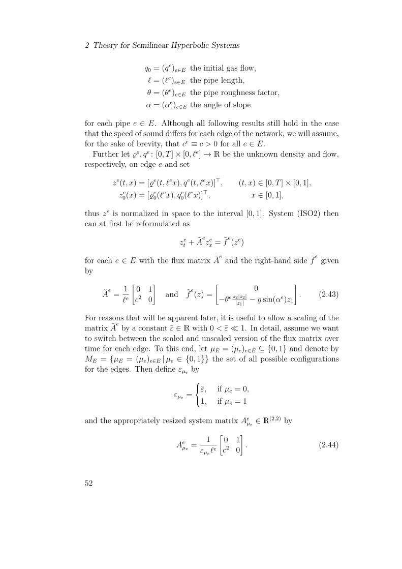
2 Theory for Semilinear Hyperbolic Systems
q0 = (qe)e∈E the initial gas flow,ℓ = (ℓe)e∈E the pipe length,θ = (θe)e∈E the pipe roughness factor,α = (αe)e∈E the angle of slope
for each pipe e ∈ E. Although all following results still hold in the casethat the speed of sound differs for each edge of the network, we will assume,for the sake of brevity, that ce ≡ c > 0 for all e ∈ E.
Further let ϱe, qe : [0, T ]× [0, ℓe]→ R be the unknown density and flow,respectively, on edge e and set
ze(t, x) = [ϱe(t, ℓex), qe(t, ℓex)]⊤, (t, x) ∈ [0, T ]× [0, 1],ze
0(x) = [ϱe0(ℓex), qe
0(ℓex)]⊤, x ∈ [0, 1],
thus ze is normalized in space to the interval [0, 1]. System (ISO2) thencan at first be reformulated as
zet + A
eze
x = fe(ze)
for each e ∈ E with the flux matrix Ae and the right-hand side f
e givenby
Ae = 1
ℓe
[0 1c2 0
]and f
e(z) =[
0−θe z2|z2|
|z1| − g sin(αe)z1
]. (2.43)
For reasons that will be apparent later, it is useful to allow a scaling of thematrix A
e by a constant ε ∈ R with 0 < ε≪ 1. In detail, assume we wantto switch between the scaled and unscaled version of the flux matrix overtime for each edge. To this end, let µE = (µe)e∈E ⊆ 0, 1 and denote byME = µE = (µe)e∈E |µe ∈ 0, 1 the set of all possible configurationsfor the edges. Then define εµe by
εµe =
⎧⎨⎩ε, if µe = 0,
1, if µe = 1
and the appropriately resized system matrix Aeµe∈ R(2,2) by
Aeµe
= 1εµeℓ
e
[0 1c2 0
]. (2.44)
52

2.3 Gas Networks
The (ISO2)-model is recovered for µe = 1, i.e., εµe = 1. We find thatAe
µeis a regular, diagonalizable matrix with the eigenvalues ± εµe c
ℓe . Set thematrices of left and right eigenvectors
Le =√
1 + c2
2c
[c −1c 1
]and Re = 1√
1 + c2
[1 1−c c
],
then LeRe = ReLe = 1 and LeAeµe
Re = diag(− cεµe ℓe , c
εµe ℓe ). Obviously, wenow can choose
Aµ =⨂e∈E
Aeµe
, L =⨂e∈E
Le and R =⨂e∈E
Re,
then Aµ, L, R not only satisfy Assumption 2.1.1(i) from Section 2.1 foreach fixed µ ∈ ME, but are smooth – in fact, constant – as functionsof (t, x) ∈ Ω as well. Note that, if the gas network contains multiplepipes with the same ratio of sound speed to pipe length, then there mightbe eigenvalues of higher multiplicity, i.e., Aµ is not strictly hyperbolic ingeneral. For e ∈ E, the characteristic variables w = (we
1, we2)e∈E are given
by
we1(t, x) =
√1 + c2
2c(cze
1(t, x)− ze2(t, x)),
we2(t, x) =
√1 + c2
2c(cze
1(t, x) + ze2(t, x)),
(2.45)
the outgoing characteristic values are we,−(t) = [we1(t, 0), we
2(t, 1)]⊤ andthe ingoing characteristic values are we,+(t) = [we
1(t, 1), we2(t, 0)]⊤ for all
t ∈ [0, T ] and all x ∈ [0, 1].The full right-hand side in (ISO2) for each e ∈ E is given by f
e in (2.43).While this is a continuously differentiable function for z1 = 0, we also seethat f
e is not globally Lipschitz-continuous and not even well-defined forz1 = 0. In fact, the (ISO2)-model is derived under the assumptions thatboth the density ϱ and the flow q remain within physically accurate bound-aries and that the density, in particular, remains positive. This is not cleara priori and in fact turns out to be a source of instability in the numericalrealisation, see Remark 4.1.2 for a more detailed discussion. We can, how-ever, avoid these technical issues by the following cut-off argument: firstintroduce for any δ > 0 the C1-cut-off-function ηδ : R→ R given by
ηδ(x) =
⎧⎪⎪⎪⎨⎪⎪⎪⎩0, x ≤ −δ,14δ
x2 + 12x + δ
4 , x ∈ (−δ, δ),x, x ≥ δ,
η′δ(x) =
⎧⎪⎪⎪⎨⎪⎪⎪⎩0, x ≤ −δ,12δ
x + 12 , x ∈ (−δ, δ),
1, x ≥ δ.
53

2 Theory for Semilinear Hyperbolic Systems
It is easy to see that ηδ is a continuously differentiable approximation ofthe function x ↦→ max0, x, which is its uniform limit for δ 0. In fact,both functions differ only on the subset (−δ, δ).
−δ δ
δ
x
ηδ(x)
−δ δ
1
x
η′δ(x)
Figure 2.5: The cut-off function ηδ and its derivative.
Further define the modified right-hand side
f e1 (z) =
[0
−θe q−ηδ(q−|z2|)ϱ+ηδ(|z1|−ϱ)z2 − g sin(αe)z1
](2.46)
with ϱ > 0 denoting a minimum density and q > 0 denoting a maximumflow. The idea then is the following: if the (ISO2)-model with its right-hand side replaced by f e
1 has a solution for a δ > 0 small enough and if thissolution actually has values ϱ > ϱ and q < q, then the same functions alsosolve the original system (ISO2). On the other hand, if the boundariesϱ > ϱ and q < q are violated by the solution of the modified system,then the same is true for the solution of the original system. Therefore,if our aim is to generate a solution inside the physical boundaries of themodel anyway, we can as well work with the above modifications. To thisend, assume δ < minϱ, q, then f e
1 again is a C1-function. This is clearfor |z2| > q − δ, since f e
1 then is the composition of C1-functions. For|z2| ≤ q − δ, we note that
(q − ηδ(q − |z2|))z2 = (q − (q − |z2|))z2 = |z2|z2
is a C1-function, too. Moreover, it is easy to see that f e1 is linearly bounded,
i.e.,
|f e1 (z)| ≤ Lf max|z1|, |z2| with Lf = max
θe q
ϱ, g sin(αe)
.
54

2.3 Gas Networks
Therefore, f e1 not only satisfies Assumption 2.1.1(ii), but also the C1-
condition in Assumption 2.1.10.In order to incorporate model (ISO-ALG) into the formulation (IBVP)
as well, we describe it as the limit of appropriately perturbed semilinearhyperbolic dynamics. To this end, we note that, after a linear transfor-mation, model (ISO2) can be written in its characteristic variables w in(2.45) as the partially diagonalized system
wt(t, x)+Dwx(t, x) = g(w(t, x)), D =[−c 00 c
], (t, x) ∈ (0, T )×(0, L),
with g : Rn → Rn defined appropriately, see (2.2). Let us assume forthe moment that g : R2 → R2 is globally Lipschitz-continuous. The sametransformation applied to (ISO3), together with given boundary valuesw1 ∈ C([0, T ],R2) yields the ODE-system
Dwx(t, x) = g(w(t, x)), (t, x) ∈ (0, T )× (0, L),w1(t, 1) = w1
1(t), t ∈ [0, T ],w2(t, 0) = w1
2(t), t ∈ [0, T ].(2.47)
To define an appropriate hyperbolic system to approximate (2.47), forε > 0 and any initial values w0 ∈ L1([0, L],R2) we set up the auxiliarysystem
εwt(t, x) + Dwx(t, x) = εD−1g(w(t, x)), (t, x) ∈ (0, T )× (0, L),w(0, x) = w0(x), x ∈ (0, L),w1(t, 1) = w1
1(t), t ∈ [0, T ],w2(t, 0) = w1
2(t), t ∈ [0, T ].
(2.48)
We then get the following result:Lemma 2.3.1.For any ε > 0 there is a unique solution w ∈ C([0, T ] × [0, L],R2) to(2.47) and a unique broad solution w : [0, T ]× [0, L] → R2 to (2.48). Therestriction of w to the set
Ω = (t, x) ∈ [0, T ]× [0, L] |L− cεt < x < c
εt
is a continuous function. Furthermore, for any t0 ∈ (0, T ) the function w
converges uniformly on [t0, T ]× [0, L] for ε 0 to w, i.e.,
limε0
sup(t,x)∈[t0,T ]×[0,L]
|w(t, x)− w(t, x)| = 0.
55

2 Theory for Semilinear Hyperbolic Systems
Proof. The global existence and uniqueness of w follows by the well-knowntheorem by Picard-Lindelöf. For (t, x) ∈ Ω, the broad solution w can bewritten as
w1(t, x) = w11(t− ε
c(L− x)) +
∫ t
t− εc
(L−x)−1
cg1(w(s, x + c
ε(t− s))) ds,
w2(t, x) = w12(t− ε
cx) +
∫ t
t− εc
x
1cg2(w(s, c
ε(t− s))) dy.
Its existence and the continuity on Ω follows from Theorem 2.1.6. Givena fixed t0 ∈ (0, T ), we obviously can choose ε small enough such that[t0, T ]× [0, L] ⊆ Ω. We then have
w2(t, x) = w12(t− ε
cx) +
∫ t
t− εc
x
1cg2(w(s, c
ε(t− s))) dy
→ w12(t) +
∫ x
01cg2(w(s, y)) dy
= w2(t, x)
for ε 0 and all (t, x) ∈ [t0, T ] × [0, L]. The convergence is uniform,since both w1
2 and g2(w) are continuous and defined on a compact set,thus uniformly continuous. The same argumentation holds for w1.
Retransforming (2.48) back to the original variables ϱ and q, we get
ϱt + 1ε
qx = − θ
c2q − ηδ(q − |q|)ϱ + ηδ(|ϱ| − ϱ)q + g sin(αe)
c2 ϱ,
qt + c2
εϱx = 0.
(2.49)
By Lemma 2.3.1, this system yields an approximation to model (ISO3) bya hyperbolic system with the same system matrix Aε
µeas in (2.44), but
with the modified right-hand side
f e0 (z) =
[− θ
c2q−ηδ(q−|z2|)ϱ+ηδ(|z1|−ϱ)z2 + g sin(αe)
c2 z1
0
]. (2.50)
We will use system (2.49) for a fixed ε > 0 with ε ≪ 1 to replace the(ISO3)-model in our applications. Again, the function f e
0 satisfies Assump-tion 2.1.1 and the C1-condition in Assumption 2.1.10. Set z = (ze)e∈E,z0 = (ze
0)e∈E and fµ = (f eµe
)e∈E.
56

2.3 Gas Networks
For each v ∈ V , additional coupling conditions accrue according to theirrespective type as described in Section 1.2 and, if v is an active element,then these coupling conditions can switch over time. Assume each node v
can have on of the configurations µv ∈ 1, . . . , 5, where
µv = 1 ⇐⇒ v is a junction node,
µv = 2 ⇐⇒ v is an open valve,
µv = 3 ⇐⇒ v is a closed valve,
µv = 4 ⇐⇒ v is an inactive compressor,µv = 5 ⇐⇒ v is an active compressor
and let MV = (µv)v∈V |µv ∈ 1, . . . , 5 ∀ v ∈ V be the set of all possibleconfigurations of the nodes in the network. We then define Cv
µv: [0, T ] ×
Rn ×Rn → R|δv| and ϕvµv
: [0, T ]→ R|δv| as follows:
• if µv = 1, i.e., v is a junction with δv = (e1, . . . , ek) and outflow qv,then
Cvµv
(t, z(t, 0), z(t, 1)) =
⎡⎢⎢⎢⎢⎢⎢⎢⎣
ze11 (t, x(v, e1))− ze2
1 (t, x(v, e2))ze2
1 (t, x(v, e2))− ze31 (t, x(v, e3))
...z
ek−11 (t, x(v, ek−1))− zek
1 (t, x(v, ek))∑e∈δ+v ze
2(t, 1)−∑e∈δ−v ze2(t, 0)
⎤⎥⎥⎥⎥⎥⎥⎥⎦ (2.51)
and ϕvµv
(t) = [0, . . . , 0, qv(t)]⊤. If v is a boundary node with δv = efor a single edge e ∈ E, then (2.51) reduces to a Dirichlet-conditionfor the flow, i.e.,
Cvµv
(t, z(t, 0), z(t, 1)) =
⎧⎨⎩ze2(t, 1), if e ∈ δ+v,
−ze2(t, 0), if e ∈ δ−v
(2.52)
and ϕvµv
(t) = qv(t).
• if µv = 2, i.e., v is an open valve, then Cvµv
is the same as forjunctions, but qv
µv≡ 0.
• if µv = 3, i.e., v is a closed valve with δv = (e1, . . . , ek), then
Cvµv
(t, z(t, 0), z(t, 1)) =
⎡⎢⎢⎢⎢⎢⎣ze1
2 (t, x(v, e1))ze2
2 (t, x(v, e2))...
zek2 (t, x(v, ek))
⎤⎥⎥⎥⎥⎥⎦ (2.53)
57

2 Theory for Semilinear Hyperbolic Systems
and qvµv≡ 0.
• if µv = 4, i.e., v is an inactive compressor, then Cvµv
is the sameas for junctions, but qv
µv≡ 0.
• if µv = 5, i.e., v is an active compressor with δ+v = e1 andδ−v = e2, where the compression is directed from e1 to e2, then
Cvµv
(t, z(t, 0), z(t, 1)) =[γ(t)ze1
1 (t, 1)− ze21 (t, 0)
ze12 (t, 1)− ze2
2 (t, 0)
](2.54)
and qvµv≡ 0. Here, γ ∈ C1([0, T ],R) is a given compression func-
tion, assumed to be globally Lipschitz-continuous and with values in[1,∞). One possibility is the compression factor stated in (1.4) fora given adiabatic Head Had ∈ C1([0, T ], [0,∞)). If we assume thatHad is bounded and globally Lipschitz-continuous, we can set
γ(t) =(
1 + Had(t)(κ− 1)RTZκ
) κκ−1
. (2.55)
Of course, other models are imaginable, too. In our applications,we will mostly make the simplifying assumption that γ in fact is aconstant function.
Finally, define Cµ : [0, T ] × R2n × R2n → R2n and ϕµ : [0, T ] → R2n foreach µ ∈MV by
Cµ(t, z0, z1) = (Cvµv
(t, z0, z1))v∈V , (t, z0, z1) ∈ [0, T ]×R2n×R2n,
ϕµ(t) = (ϕvµv
(t))v∈V , t ∈ [0, T ].(2.56)
Then we have the following result:Lemma 2.3.2 (Well-posed Coupling Conditions).For any µ ∈ MV , let Cµ and ϕµ be the functions defined in (2.56). ThenCµ ∈ C1([0, T ]×R2n×R2n,R2n) and Assumption 2.1.1(iii) is satisfied.
Proof. Both (2.51) and (2.53) are obviously linear, therefore smooth andglobally Lipschitz-continuous functions. Since γ is assumed to be contin-uously differentiable, so is (2.54). Since γ, furthermore, is assumed to bebounded and globally Lipschitz continuous, it is easy to see that (2.54) isglobally Lipschitz as well.
58

2.3 Gas Networks
It remains to show that, in each of these cases, the ingoing characteristicsat the node are uniquely mapped to the outgoing characteristics for anyfixed time point t ∈ [0, T ]. To this end, note that (2.51) is equivalent to
we11 (t, x(v, e1)) + we1
2 (t, x(v, e1)) = we21 (t, x(v, e2)) + we2
2 (t, x(v, e2))= . . .
= wek1 (t, x(v, ek)) + wek
2 (t, x(v, ek))
and√
1 + c2
cqv(t) =
∑e∈δ+v
(we1(t, 1)− we
2(t, 1))−∑
e∈δ−v
(we1(t, 0)− we
2(t, 0)).
If we assume the values w−(t) = [(we1(t, 0))e∈δ−v, (we
2(t, 1))e∈δ+v]⊤ to begiven, these conditions define a linear system in the variables w+(t) =[(we
2(t, 0))e∈δ−v, (we1(t, 1))e∈δ+v]⊤. First set
wv(t) = 2|δv|
⎛⎝ ∑e∈δ+v
we2(t, 1) +
∑e∈δ−v
we1(t, 0) +
√1 + c2
cqv(t)
⎞⎠ , (2.57)
then the unique solution is given by
we2(t, 0) = −we
1(t, 0) + wv(t) for all e ∈ δ−v, (2.58)we
1(t, 1) = −we2(t, 1) + wv(t) for all e ∈ δ+v. (2.59)
Next, (2.53) is equivalent to
we1(t, x(v, e)) = we
2(t, x(v, e)) ∀ e ∈ δv,
therefore w+(t) = w−(t). Finally, (2.54) is equivalent to
we21 (t, 0) + we2
2 (t, 0) = γ(t)(we11 (t, 1) + we1
2 (t, 1)),we2
1 (t, 0)− we22 (t, 0) = we1
1 (t, 1)− we12 (t, 1).
For given values we12 (t, 1), we2
1 (t, 0), we can solve for we11 (t, 1) and we2
2 (t, 0)and get [
we11 (t, 1)
we22 (t, 0)
]=[γ(t) −1−1 −1
]−1 [−γ(t) 1−1 −1
] [we1
2 (t, 1)we2
1 (t, 0)
], (2.60)
which is well-defined, since we assumed that γ(t) ≥ 1 for all t ∈ [0, T ].This completes the proof.
59

2 Theory for Semilinear Hyperbolic Systems
Remark 2.3.3 (Nonlinear Compressor Model).Although, for brevity, we will use the compression ratio (2.55) under theassumption that Had : [0, T ]→ [0,∞) is known, the results in Lemma 2.3.2(and therefore those in the upcoming Theorem 2.3.4) can as well be shownfor the explicitly flow-dependent model
γ(t, ze1(t, 1), ze2(t, 0)) =(
1 + ηPcomp(t)(κ− 1)(q0 + ηδ(qe1(t, 1)− q0))RTZκ
) κκ−1
, (2.61)
where v ∈ V is a compressor node with δ+v = e1, δ−v = e2 andze = (ϱe, qe)⊤ for e ∈ E. Here, Pcomp ∈ C1([0, T ], [0,∞)), η, R, T, Z > 0and κ > 1 all are fixed parameters. Note that, in comparison to themodel in (1.3), we need to add a cut-off function ηδ to guarantee that thedenominator won’t be zero, q0 ∈ (0, 1) and δ > 0 can be chosen small. Toshow the well-posedness of the coupling conditions
ϱe2(t, 0) = γ(t, ze1(t, 1), ze2(t, 0))ϱe1(t, 1),qe2(t, 0) = qe1(t, 1),
(2.62)
we then can proceed as in the proof of Lemma 2.3.2 and assume that t ∈ T
and the ingoing characteristics we12 (t, 1) and we2
1 (t, 0) are given and fixed.If γ ≥ 1 is a guess for the correct value of the compression ratio γ, thenthe outgoing characteristics are given by (2.60). Transforming back to theoriginal variables yields[
ϱe1(t, 1)qe1(t, 1)
]= 2
1 + γ
1√1 + c2
[1 1γc −c
] [we1
2 (t, 1)we2
1 (t, 0)
],[
ϱe2(t, 0)qe2(t, 0)
]= 2
1 + γ
1√1 + c2
[γ γ
γc −c
] [we1
2 (t, 1)we2
1 (t, 0)
].
Of course, for arbitrary ratios γ, these values in general will not satisfy(2.62). Instead, we can set up an update
γk+1 = Φ(γk)
= γ
(t,
21 + γk
[1 1
γkc −c
] [we1
2 (t, 1)we2
1 (t, 0)
],
21 + γk
[γk γk
γkc −c
] [we1
2 (t, 1)we2
1 (t, 0)
])
=⎛⎝1 + h(t)
(q0 + ηδ( 2c1+γk (γkwe1
2 (t, 1)− we21 (t, 0))− q0))
⎞⎠ κκ−1
60

2.3 Gas Networks
for a suitably defined h : [0, T ] → [0,∞) and k ∈ N0 with γ0 = γ. Toprove the well-posedness of (2.62), it suffices to show that the such definedfunction Φ has a unique fixed point in [1,∞). This, however, can be easilyseen after we note that Φ([1,∞)) ⊆ [1,∞) with Φ(1) > 1 and Φ′(γ) < 0for all γ ∈ [1,∞).
Since we only want to switch the states of valves between open andclosed and those of compressors between inactive and active, we have theconstraint set
QV =(µV , µ′
V ) ∈MV | (µv ∈ 2, 3 ∧ µ′v ∈ 2, 3)
∨ (µv ∈ 4, 5 ∧ µ′v ∈ 4, 5) ∀ v ∈ V
There are no restrictions on how to switch ME, thus we can set QE =ME ×ME. Combining both, we set
M = ME ⊗MV and Q = QE ⊗QV
and define T N(0, T ) and MN as in (2.34) and (2.35). In summary, anyswitching schedule (τ, µ) ∈ T N(0, T ) ×MN yields the complete networkmodel including switching models and switching coupling conditions
zt(t, x) + Aµkzx(t, x) = fµk(z(t, x)), (t, x) ∈ (τk, τk+1)× (0, 1),z(0, x) = z0(x), x ∈ [0, 1],
Cµk(t, z(t, 0), z(t, 1)) = ϕµk(t), t ∈ (τk, τk+1),k ∈ 0, . . . , N.
(NET)
We now can apply both Theorem 2.1.6 and Theorem 2.1.11 to get thefollowing results on existence, uniqueness and regularity of the switchedgas network system:Theorem 2.3.4 (Solution to the Switched Gas Network Model).For each µ ∈M , the triple (Aµ, fµ, Cµ) satisfies both Assumption 2.1.1 andAssumption 2.1.10. Therefore, given p ∈ [1,∞), any z0 ∈ Lp([0, 1],R2n)and any ϕ ∈ Lp([0, T ],R2n), system (NET) has a unique broad solution
z ∈ C([0, T ], Lp([0, 1],R2n)).
If z0 and ϕ are essentially bounded, then so is z. If there are sequences0 < x1 < . . . < xNx < 1 and 0 < t1 < . . . < tNt < 1 such that
z0 ∈Nx⨁j=1
C1([xj−1, xj],Rn) and ϕ ∈Nt⨁
j=1C1([tj−1, tj],Rn),
61

2 Theory for Semilinear Hyperbolic Systems
then
z ∈N0⨁j=1
C0(ω0j ,Rn) ∩
N1⨁j=1
C1(ω1j ,Rn)
with (ω0j )j=1,...,N0 and (ω1
j )j=1,...,N1 as in Theorem 2.1.11.
Concerning the semigroup property of the solution operator, we of coursecan apply Theorem 2.1.15 for any fixed choice of µ ∈ M and an affine-linear variant of the above model. To match the usual semigroup notation,we now write z : [0, T ] → Lp([0, 1],R2n) as a function mapping each timepoint t ∈ [0, T ] to a Lp-function defined on the network and formally letϕ : [0, T ] → Lp([0,∞),R2n) be a function with ϕ(0, s) = (qv(s))v∈V fors ∈ [0,∞), where qv is for each v ∈ V continued by zero for all timess ∈ [0,∞). We denote
Z = Lp([0, 1],R2n)× Lp([0,∞),R2n).
In order to satisfy Assumption 2.1.14, we now need to assume that thecompression function γ ≡ γ in (2.54) for each compressor node is actuallyconstant with a fixed value γ > 0, then obviously each of the coupling func-tions defined in (2.51), (2.53) and (2.54) is linear and time independent.In fact, with an appropriate choice of factors β = (β0, β1) ∈ (0,∞)(n,2),the coupling conditions can be formulated for a function pair (z, ϕ) ∈ Z
as the system of linear equations
βex(v,e)z
e1(x(v, e)) = βe′
x(v,e′)ze′
1 (x(v, e′)) ∀ e, e′ ∈ δv, (2.63)∑e∈δ+v
ze2(1)−
∑e∈δ−v
ze2(0) = qv(0) (2.64)
for all v ∈ V . This is equivalent to setting
Cv(t, z(t, 0), z(t, 1)) =
⎡⎢⎢⎢⎢⎢⎣βe1
x(v,e1)ze11 (x(v, e1))− βe2
x(v,e2)ze21 (x(v, e2))
...β
ej−1x(v,ej−1)z
ej−11 (x(v, j − 1))− β
ej
x(v,ej)zej
1 (x(v, ej))∑e∈δ+v ze
2(1)−∑e∈δ−v ze2(0)
⎤⎥⎥⎥⎥⎥⎦ ,
(linCPL)for each v ∈ V , where δv = (e1, . . . , ej). We will refer to the combinedsystem (NET), (linCPL) in the following, when we want to assume thatlinearized coupling conditions are used. Similar to (2.29) and (2.30), we
62

2.3 Gas Networks
thus define the domainD(H) = (z, ϕ) ∈ Lp([0, 1],R2n)× Lp([0,∞),R2n) |
z = (ze)e∈E, ϕ = (qv)v∈V are absolutely continuousand satisfy (2.63), (2.64) for all v ∈ V
(2.65)
and the operator H : D(H)→ Z by
H(z, ϕ) =[−Aµ 0
0 1
] [zx
ϕs
]. (2.66)
We can apply Theorem 2.1.15 to find that H is the generator of a C0-semigroup. This semigroup has a locally explicit representation, as thefollowing result shows:Theorem 2.3.5 (Semigroup for (ISO2) on Networks).For any fixed µ ∈M , the operator (D(H), H) defined in (2.65) and (2.66)is the infinitesimal generator of a C0-semigroup S(t)t≥0 on Z. Setλe = c
εeµe ℓe for each e ∈ E and T := min 1
λe | e ∈ E. Given initial data(z0, ϕ0) ∈ D(H), the value (z(t), ϕ(t)) = S(t)(z0, ϕ0) can be constructedexplicitly on [0, T ]× [0, 1] as follows: set
βv =∑
e∈δ+v
βe1c +
∑e∈δ−v
βe0c (2.67)
ϱv(t) = 1βv
⎡⎣ ∑e∈δ+v
[c
1
]⊤
ze0(1− λet) +
∑e∈δ−v
[c
−1
]⊤
ze0(λet) + ϕv
0(t)⎤⎦ (2.68)
for each v ∈ V and
ze(t, 0) =[
1−c
]βe
0ϱe(1)(t)−[01
] [−c
1
]⊤
ze0(λet), (2.69)
ze(t, 1) =[1c
]βe
1ϱe(2)(t)−[01
] [c
1
]⊤
ze0(1− λet) (2.70)
for each e ∈ E, then ϕ(t, s) = ϕ0(t + s) for all (t, s) ∈ [0, T ]× [0,∞) and
ze(t, x) = 12
[1 1
c
c 1
]ze
∗ (t, x) + 12
[1 −1
c
−c 1
]ze
∗ (−t, x) (2.71)
for (t, x) ∈ [0, T ]× [0, 1], where
ze∗(t, x) =
⎧⎪⎪⎪⎨⎪⎪⎪⎩ze
0 (x− λet) , if x− λet ∈ [0, 1],ze(t− 1
λe x, 0)
, if x− λet < 0,
ze(−t− 1
λe (1− x), 1)
, if x− λet > 1.
(2.72)
63
2 Theory for Semilinear Hyperbolic Systems
Proof. It is easy to see that, since z0 and ϕ0 are absolutely continuous, soare ϕ(t, ·) and z(t, ·) for t ∈ [0, T ]. In fact, one immediately checks that
limt0
ϱe(1)(t) = limx0
ze0(x) and lim
t0ϱe(2)(t) = lim
x1ze
0(x),
thus ze∗ in (2.72) is continuous and piecewise absolutely continuous, there-
fore absolutely continuous. From (2.69) and (2.70), we get ze1(t, 0) =
βe0ϱe(1)(t) and ze
1(t, 1) = βe0ϱe(2)(t), thus the first coupling condition (2.63)
is satisfied. Moreover, for each v ∈ V we have∑e∈δ+v
ze2(t, 1)−
∑e∈δ−v
ze2(t, 0)
=∑
e∈δ+v
⎡⎣βe1cϱe(2)(t)−
[c
1
]⊤
ze0(1− λet)
⎤⎦−
∑e∈δ−v
⎡⎣−βe0cϱe(1)(t) +
[c
−1
]⊤
ze0(λet)
⎤⎦=⎛⎝ ∑
e∈δ+v
βe1c +
∑e∈δ−v
βe0c
⎞⎠ ϱv(t)
−∑
e∈δ+v
[c
1
]⊤
ze0(1− λet)−
∑e∈δ−v
[c
−1
]⊤
ze0(λet)
= βvϱv(t)− (βvϱv(t)− qv(t))= qv(t),
thus condition (2.64) holds, too. It remains to show that (z, ϕ) satisfy thedifferential equation [
zt
ϕt
]= H
[z
ϕ
].
This is obvious for ϕ, since ϕt−ϕx = 0 is the well-known linear transportequations. Further note that (ze
∗)t = λe(ze∗)x for all e ∈ E. For ze, we thus
find
Aezex(t, x) = 1
2εeµe
ℓe
[0 1c2 0
] [1 1
c
c 1
](ze
∗)x(t, x)
+ 12εe
µeℓe
[0 1c2 0
] [1 −1
c
−c 1
](ze
∗)x(−t, x)
64
2.3 Gas Networks
= cλe
2εeµe
ℓe
[1 1
c
c 1
](ze
∗)t(t, x) + cλe
2εeµe
ℓe
[1 −1
c
−c 1
](ze
∗)t(−t, x)
= zet (t, x)
for a.e. (t, x) ∈ (0, T )× (0, 1). This completes the proof.
Remark 2.3.6 (Continuation of the Construction).Utilising the semigroup property
S(t + s)(z0, ϕ0) = S(t)S(s)(z0, ϕ0) ∀ t, s ≥ 0, (z0, ϕ0) ∈ Z,
the construction in Theorem 2.3.5 can be repeated successively for thetime intervals [jT , (j + 1)T ] for j ∈ N. Remark 2.3.7 (Energy Methods and the Friction Term).If z ∈ C1(Ω,R2n) with ze(t, x) = (ϱe(t, ℓex), qe(t, ℓex))⊤ for all (t, x) ∈ Ωis a classical solution to system (NET) with the linear coupling conditions(linCPL), then there also are energy methods available to examine thestability of the system. For instance, in the case that the (ISO2)-model issolved on a network of horizontal pipes, i.e., εe = 1 and αe = 0 for e ∈ E,introduce the energy function
E(t) = 12∑e∈E
∫ 1
0[(ϱe)2(t, ℓex) + 1
c2 (qe)2(t, ℓex)] dx. (2.73)
Then
d
dtE(t) =
∑e∈E
∫ 1
0(ϱe(t, ℓex)ϱe
t (t, ℓex) + 1c2 qe(t, ℓex)qe
t (t, ℓex)) dx
=∑e∈E
∫ 1
0
(− ϱe(t, x)qe
x(t, x)− qe(t, x)ϱet (t, x)
− θe (qe)2(t, x)|qe(t, x)||ϱe(t, x)|
)dx
(∗)≤∑e∈E
∫ 1
0(−ϱe(t, x)qe
x(t, x) + qex(t, x)ϱe(t, x))dx
−∑e∈E
(ϱe(t, 1)qe(t, 1)− ϱe(t, 0)qe(t, 0))
=∑v∈V
⎡⎣− ∑e∈δ+v
ϱe(t, ℓe)qe(t, ℓe) +∑
e∈δ−v
ϱe(t, 0)qe(t, 0)⎤⎦
65

2 Theory for Semilinear Hyperbolic Systems
=∑v∈V
ϱv(t)⎡⎣− ∑
e∈δ+v
βe1qe(t, ℓe) +
∑e∈δ−v
βe0qe(t, 0)
⎤⎦where in (∗) we used partial integration and the fact that
−θq2|q|
ϱ≤ 0 ∀ (ϱ, q) ∈ (0,∞)×R.
If βe0 = βe
1 = 1 for all e ∈ E, we especially get
d
dtE(t) =
∑v∈V
−ϱv(t)qv(t),
thus if qv ≥ 0, i.e., if there is no flow into the system at any node, theenergy is monotonically decreasing. In this sense, the right-hand side infact has at least a non-increasing effect on the solution, so calling it afriction term is justified. Example 2.3.8 (The Y-network).Consider the junction network or Y-network shown in Figure 2.6 withnodes V = (v1, v2, v3, v4) and edges E = (e1, e2, e3), where e1 = (v1, v2),e2 = (v2, v3) and e3 = (v2, v3). For this example, we use the simplerindexing zej = zj for j = 1, 2, 3 and also allow different speeds of soundsc1, c2, c3 > 0 per edge. We set εj = 1 for all j and neglect the right-hand
•v1
•v2
•v3
•v4
e1
e2
e3
Figure 2.6: The Y-network.
66

2.3 Gas Networks
side, then system (NET) becomes
zjt (t, x) +
[0 1c2
j 0
]zj
x(t, x) = 0, t ∈ (0, T ), x ∈ (0, ℓj),
zj(0, x) = zj0(x), x ∈ [0, 1]
(2.74)
for each j with zj = (ϱj, qj)⊤ and a given initial state zj0 = (ϱj
0, qj0)⊤. The
boundary conditions (linCPL) here reduce to
β1ϱ1(t, 1) = β2ϱ2(t, 0) = β3ϱ3(t, 0),q1(t, 1)− q2(t, 0)− q3(t, 0) = qv(t),
q1(t, 0) = 0,
q2(t, 1) = 0,
q3(t, 1) = 0
(2.75)
for certain β1, β2, β3 > 0. We have seen in the proof of Lemma 2.3.2how these coupling conditions map all ingoing characteristics at v2 to therespective outgoing characteristics. In fact, if we are given at any timepoint t ∈ [0, T ] the values w1
+, w2−, w3
− of the characteristics ingoing at v2,set
c = c1
β1+ c2
β2+ c3
β3,
ϱ = 1c
⎡⎢⎢⎣1
β11
β21
β3
⎤⎥⎥⎦⎡⎢⎣2
⎡⎢⎣c1w1+
c2w2−
c3w3−
⎤⎥⎦−⎡⎢⎣111
⎤⎥⎦ qv2(t)
⎤⎥⎦⊤
,
then the values for ϱ and q at the node v2 are given by
β1ϱ1(t, 1) = β2ϱ
2(t, 0) = β3ϱ3(t, 0) = ϱ,
q1(t, 1) = c1(2w1+(t)− ϱ),
q2(t, 0) = c2(ϱ− 2w2−(t)),
q3(t, 0) = c3(ϱ− 2w3−(t)).
Similar formulae hold for nodes with more than 3 incident edges. They areuseful in examining the behaviour of shocks at nodes, compare Figure 2.7for an example with β1 = β2 = β3 = 1.
As soon as a jump discontinuity travelling along edge e1 reaches thenode v2, it is split and reflects new jumps along each incident edge. For
67

2 Theory for Semilinear Hyperbolic Systems
• •
•
•
v1 v2
v3
v4
e1
e2
e3
%
(a) Ingoing single density shock
• •
•
•
v1 v2
v3
v4
e1
e2
e3
%
(b) Outgoing split density shocks
• •
•
•
v1 v2
v3
v4
e1
e2
e3
q
(c) Ingoing single flow shock
• •
•
•
v1 v2
v3
v4
e1
e2
e3
q
(d) Outgoing split flow shocks
Figure 2.7: Shock behaviour at a node with 3 incident edges.
both density and flux, the new jumps have to be chosen in a way such thatthe boundary conditions are satisfied immediately after again. Note that,if there are more than two incident edges at a node, then jump discontinu-ities from an edge e are not only passed over to the other edges, but alsopartially reflected back on e itself in general. In this way, an originallysingle jump discontinuity multiplies each time it passes a node and canthus produce arbitrary many new jumps, if the time horizon is sufficientlylarge. The height of the new jumps, however, is smaller than that of theoriginal jump and keeps decreasing with any further reflection. From anumerical point of view, where smearing and damping effects at jumpsare often unavoidable anyway, this means that, if the network under con-sideration has a sufficiently high connectivity, then a jump discontinuityonce introduced to the system is negligible after a short time. The fric-
68

2.3 Gas Networks
tion term of the (ISO2)-model damps the height of jump discontinuitiesadditionally. This also means, however, that wave tracking methods areproblematic and that finite-volume schemes are the method of choice, seeChapter 4.
We finally want to discuss an application of the results from Section 2.2to the example of gas networks. In detail, we present a well-posednessresult for check valves in networks. Check valves are a special kind ofvalves, meant to allow throughput of gas in one direction, but to preventflow against it. These elements usually are used to protect other activecomponents of the gas network from damage or to direct gas transporton certain routes through a network. In contrast to other valves that, inprincipal, can be modelled with more than two adjacent edges, we assumethat check valves have exactly one ingoing edge and one outgoing edge,defining uniquely a prescribed admissible flow direction from the ingoingto the outgoing edge. They are modelled just like valves with the onlydifference that they are not operated by arbitrary switching decisions, butby state-dependent feedback rules. In detail, we want to assume that anopen check valve closes as soon as there is gas flow against the prescribedflow direction, and that a closed check valve opens again as soon as thedifference in gas densities is high enough.
Suppose we are given a subset of nodes V ⊆ V that are check valves.For each node v ∈ V with δ+v = e1 and δ−v = e2, introduce theswitching rules
(hv)23(t, z(t, 0), z(t, 1)) = ze2
2 (t, 0), (2.76)(hv)3
2(t, z(t, 0), z(t, 1)) = ze21 (t, 0)− ze1(t, 1) + ϱv (2.77)
with a fixed threshold value ϱv > 0, i.e., the mode of the check valveswitches from open (µ = 2) to closed (µ = 3), if flux qe2(t, 0) is non-positive, and back from closed to open, if the density ϱe2(t, 0) ahead of thecheck valve is at least by the amount ϱv higher than the density ϱe2(t, 0)abaft it. We do not want to consider additional state transitions here andset
(gv)23(τ, x, z0, z1) = (gv)3
2(τ, x, z0, z1) = (z0, z1) (2.78)
for all (τ, x, z) ∈ [0, T ] × [0, 1] × R2n × R2n. Consider the system (NET)with given time-varying switching signals for all active elements other thancheck valves, then we may ask whether the switching rules (2.76) and (2.77)
69

2 Theory for Semilinear Hyperbolic Systems
generate a well-defined feedback control in the sense of Definition 2.2.5.This is in fact true as the following theorem shows:Theorem 2.3.9 (Check Valve Feedback Solution).For each v ∈ V ⊆ V let ϱv > 0. Then Theorem 2.2.10 holds for the system(NET) together with the switching rules (2.76), (2.77) and (2.78), i.e.,there is a unique feedback control (τ v, µv) for each v ∈ V . The feedbackcontrol depends continuously on z0 in the sense of Theorem 2.2.10, if thefollowing holds for each τk ∈ τ : for each v ∈ V with µv
k = µvk+1, we have
qe2t (τ−
k , 0) < 0, if µk = 2,
ϱe1t (τ−
k , 1)− ϱe2t (τ−
k , 0) < 0, if µk = 3.(2.79)
Proof. We already have seen that (NET) satisfies Assumption 2.1.10 andthe functions h2
3, h32, g2
3 and g32 are obviously smooth. The assumption for
uniqueness of the feedback control in Theorem 2.2.10 is trivially satisfied,because there are only two possible states to switch between at all. Denotefor any time point τ ∈ [0, T ]
ϱ1 = ϱe1(τ−, 1), q1 = qe1(τ−, 1),ϱ2 = ϱe2(τ−, 0), q2 = qe2(τ−, 0).
Then, the projections defined in Corollary 2.1.13 in this case are given by
P 23 (ϱ1, q1, ϱ2, q2) =
⎡⎢⎢⎢⎢⎣ϱ1 + 1
c1 q1
0ϱ2 − 1
c2 q2
0
⎤⎥⎥⎥⎥⎦when switching from µ = 2 to µ = 3 and by
P 32 (ϱ1, q1, ϱ2, q2) = 1
c1 + c2
⎡⎢⎢⎢⎢⎣c1ϱ1 + c2ϱ2
c1c2(ϱ1 − ϱ2)c1ϱ1 + c2ϱ2
c1c2(ϱ1 − ϱ2)
⎤⎥⎥⎥⎥⎦when switching from µ = 3 to µ = 2. Assumption 2.2.1(iv) holds, becausewe even have P 2
3 P 32 = P 3
2 P 23 = id, i.e., the maps P 2
3 and P 32 are inverse
70

2.3 Gas Networks
functions of one another. In order to show that no approximate fixed pointexist for this system, it suffices to observe that
g32(ϱ1, q1, ϱ2, q2) ≤ 0 ⇐⇒ ϱ1 − ϱ2 ≥ ϱv,
thusg2
3(P 32 (ϱ1, q1, ϱ2, q2)) = c1c2(ϱ1 − ϱ2) ≥ c1c2ϱv > 0
is uniformly bounded away from zero for all (ϱ1, q1, ϱ2, q2). This allows usto apply Theorem 2.2.10. Applying the conditions in Theorem 2.2.10 forthe continuous dependence of the solution on z0 yields (2.79) and completesthe proof.
71


3 Optimization for HybridSystems of AbstractEvolution Equations
In this chapter, we consider optimization theory for hybrid dynamical sys-tems. In contrast to Chapter 2, where we presented solution theory specif-ically for feedback-controlled switched systems of semilinear hyperbolicequations, we now will have a look at more abstract systems based onsemigroup theory. We have already seen that hyperbolic initial-boundaryvalue problems largely fit into this framework, at least under some rathermild, but simplifying assumptions. In detail, we now formulate hybriddynamical systems on some (not necessarily infinite dimensional) spaceZ and a finite set of modes M . For a given family Aµµ∈M of denselydefined linear operators on Z, families of nonlinear functions fµµ∈M andgµ,µ′µ,µ′∈M×M on Z and a finite time horizon [0, T ] with initial conditionz(0) = z0 ∈ Z the dynamics are governed by abstract continuous timeevolution equations combined with discrete events involving state resets
z = Aµz + fµ(z), z = gµ,µ′(z−),
whenever the mode µ ∈M is held constant or whenever µ with associatedstate z− is switched to the new mode µ′ ∈M with new state z at switch-ing times (τk)k∈N0 ⊆ [0, T ], respectively. Supposing that the sequence ofswitching times (τk)k and the modal sequence (µk)k are subject to ourcontrol and that we have a cost function J = J(z) integrating runningand switching cost associated to the respective continuous or discrete evo-lution, we may consider the minimization of J over any such sequences offinite length as an optimal control problem. The precise setting and mainhypotheses are introduced in Section 3.1 below.
This and variants of this optimal control problem have been extensivelyaddressed for ordinary differential equations (ODEs), e.g., based on dy-namic programming principles [26, 47], non-smooth programming [17],
73

3 Optimization for Hybrid Systems of Abstract Evolution Equations
control parametrization enhancing techniques [58] and relaxation tech-niques [11, 81]. Moreover, if the modal sequence (µk)k is a-priori fixed,the control problem reduces to switching-time optimization and can besolved using gradient-based methods [31, 32, 49, 88]. The latter approachhas also been extended using gradients with respect to mode-insertions intoa given sequence [32]. Switching-time optimization and mode-insertionscan be combined to conceptual algorithms to tackle the original problem[5, 86]. We refer to [90] for a more detailed survey of available results forthe ODE case.
Much less work has been done for similar optimal control problems inthe context of ordinary delay differential equations (DDEs) and partialdifferential equations (PDEs). Such problems arise for example in optimalcontrol of gas networks, where switching of valves is an essential part ofthe control mechanism for the gas flow governed by algebraically coupledPDEs on a graph representing the network of pipes [39, 40]. Switching-time optimization has been considered for ordinary DDEs in [85, 87] and,when switching only affects boundary data, for scalar hyperbolic PDEs inthe semilinear case [38] and in the non-linear case [71]. In a more abstractfashion based on semigroup theory covering both, certain DDEs and PDEs,dynamic programming extends to problems when Aµ is a generator of astrongly continuous semigroup independent of µ and switching only affectsthe non-linear perturbation [61]. In the same setting, relaxation techniquescan sometimes be applied [41].
In this chapter, we extend the concept of switching-time optimizationand mode-insertion from ODE problems in [32] to the abstract setting ofnon-linearly perturbed strongly continuous semigroups. Unlike in [32], weconsider non-autonomous dynamics, state-resets at switching times andinclude switching costs. Moreover, among switching of the non-linearperturbation, our theory explicitly considers switching of the semigroups’generator, which (in non-trivial cases) cannot be handled with the resultsavailable in the literature so far. This allows—under certain technicalrestrictions—the treatment of switching, e. g., the delay parameter of aDDEs or switching the principle part of a PDE in the hybrid dynamicalsystem represented by the above equations. Our analysis focuses on thedifferentiability properties of the cost function and the representation ofthe derivative using solutions to appropriate adjoint problems. We fur-ther present a descent optimization method for switching sequences ofhybrid systems of an alternate-direction type. In detail, the adjoint-based
74
3.1 Hybrid Systems of Abstract Evolution Equations
gradient formulae for the switching time are incorporated in a projected-gradient method to optimize the positioning of the switching sequence,which we then combine with a mode insertion step. The analysis for suchalgorithms mainly follows the preliminary work in [5].
In Section 3.1 we introduce our abstract problem setting including thehypotheses concerning the regularity of the system parameters. In Sec-tion 3.2 we consider differentiation of the costs with respect to the switch-ing times for a given mode sequence. In Section 3.3 we discuss differen-tiation of the costs with respect to the insertion of a new mode into agiven sequence of modes. In Section 3.4 we show that one can recover theresult of [32] for the ODE case from our theory under rather mild techni-cal assumptions on the system parameters. Moreover, we show that theresults can be used for example to obtain efficient gradient-representationsof integro-type DDE and that the theory is consistent with stability anal-ysis for a PDE switching between a transport equation and a diffusionequation. The application to our main example, the optimization of gasnetworks, is postponed to Chapter 4.
This chapter mainly follows the exposition of the author’s article [77].
3.1 Hybrid Systems of Abstract EvolutionEquations
As a motivation for typical problems related to hybrid or switched system,let us consider the following example with ordinary differential equations:Example 3.1.1 (Optimally Switching Gears).Let us suppose we want to accelerate a car, say with N +1 gears, from restto a fixed velocity vd. We further assume that we are speeding up perma-nently at full throttle and only disengage the clutch for instantaneouslyswitching to the next higher gear. We immediately stop accelerating assoon as we arrive at the velocity vd. The problem then is to find optimaltime points to change the gear such that the target velocity is met in min-imal time. Denote by x, v, a : [0,∞) → R the time-dependent position,velocity and acceleration, respectively, of the car, then a(·) = ak(v(·)) ingeneral also depends on the current gear k ∈ 1, . . . , N + 1, the veloc-ity and possibly other technical parameters, especially ak(v) = 0 for allv ≥ vd. Assume τ0 = 0 and τN+1 = T > 0 is an upper bound for the finaltime, further denote by τk ∈ [0, T ] the time when we switch from gear k
75
3 Optimization for Hybrid Systems of Abstract Evolution Equations
to k + 1 such that τ0 ≤ τ1 ≤ . . . ≤ τN ≤ τN+1. Denote by TN(0, T ) the setof all such vectors τ = (τk)k. Setting z = (x, v)⊤ then yields the system
z(t) =[x(t)v(t)
]=[
v(t)ak(v(t))
]=: fk(t, z(t)), t ∈ (τk, τk+1)
for every k ∈ 0, . . . , N. A possible way to enforce a maximally quickacceleration to vd is to measure the deviation of v from vd over time bythe penalty cost term
J(z) =∫ T
0
γ
2 (v(t)− vd)2 dt
for a parameter γ > 0. Under the above constraints, it is easy to see thatJ in fact is minimal if and only if v(t) = vd for a minimal t ∈ [0, T ]. Wearrive at the problem
minτ
J(z)
s.t. z(t) = fk(t, z(t)), t ∈ (τk, τk+1), k = 0, . . . , N,
z(0) = 0,
τ ∈ T N(0, T ).
Note that we also allow τk = τk+1 for any k ∈ 0, . . . , N, which can beinterpreted as skipping the gear k + 1.
There is a number of conceivable generalizations to this problem: first ofall, the optimization might also include minimizing the fuel consumptionor additional penalties for staying in one gear too long. We also couldmodel speed losses due to the disengaging, thereby taking into accountthat this process actually is not completely instantaneous, by allowing fordrops in velocity at the switching time points.
The assumption that we only switch to higher gears is quite evidentin this example, since we only wish to speed up. However, if we ratherwere interested in accelerating a car at rest and then stopping it at afinal location as fast as possible, braking processes would occur and itmight be necessary to alternate between all gears over time. Anotheraim of optimization then could be, additionally to the mere optimizationof given switching times, to determine, whether and where adding newswitching points could improve the process. The optimization then wouldbe with respect to both the position and number of switching time points.
76
3.1 Hybrid Systems of Abstract Evolution Equations
Moreover, it then might not be the best strategy to always speed up atfull throttle, but instead, to simultaneously control the acceleration overthe gas pedal. This would lead to an optimization problem combining thetime-discrete switching decisions with partially continuous controls.
In this chapter, we will derive a general framework based on semigrouptheory that allows us to handle not only the problems brought up in Ex-ample 3.1.1, but also similar questions in the context of delayed differentialequations or partial differential equations such as the systems derived inChapter 2 for gas networks.
Our basic hypotheses for this section are as follows.Assumption 3.1.2.Let Z be a reflexive Banach space and z0 ∈ Z, let M be a finite set andQ ⊆M ×M , let µ0 ∈M and further assume the following:
(i) Aµ is for each µ ∈ M the infinitesimal generator of a strongly con-tinuous semigroup of bounded linear operators Sµ(t)t≥0 on Z withdomain D(Aµ) ⊆ Z.
(ii) For every µ ∈M let fµ ∈ C1([0,∞)×Z, Z) and for every (µ, µ′) ∈ Q
let gµµ′ : Z → Z be a given map.
(iii) z0 ∈ D(Aµ0) and the map gµµ′ is continuously differentiable for all
(µ, µ′) ∈ Q with µ = µ′, satisfying the inclusion gµµ′(D(Aµ)) ⊆
D(Aµ′).
We again denote byMN the set of admissible mode sequences as definedin (2.35). The hybrid semilinear evolutions then are specified as follows:given a fixed N ∈ N0, a monotonically increasing, but not necessarilystrictly increasing sequence of switching times τ = (τk)k=0,...,N+1 ⊆ [0,∞)and a sequence of modes µ = (µk)k=0,...,N ∈MN , we consider dynamics ofthe form
z(t) = Aµkz(t) + fµk(t, z(t)), k ∈ 0, . . . , N, t ∈ (τk, τk+1),z(τ+
k ) = gµk−1µk
(z(τ−k )), k ∈ 1, . . . , N,
z(τ0) = z0.
(3.1)
A map z : [τ0, τN+1] → Z is called a mild solution to (3.1), if, for all k ∈0, . . . , N, there are functions zk : [τk, τk+1] → Z satisfying the followingconditions:
77

3 Optimization for Hybrid Systems of Abstract Evolution Equations
(i) zk is the only element of C([τk, τk+1], Z) satisfying the variation ofconstants formula
zk(t) = Sµk(t− τk)zk0 +
∫ t
τk
Sµk(t− s)fµk(s, zk(s)) ds ∀ t ∈ [τk, τk+1],
where
zk0 =
⎧⎨⎩z0, if k = 0,
gµk−1µk
(zk−1(τk)), if k ∈ 1, . . . , N.
(ii) If τk < τk+1 for some k ∈ 0, . . . , N, then z|[τk,τk+1) ≡ zk.
The map z is called a classical solution to (3.1), if, furthermore, the fol-lowing holds:
(iii) If τk < τk+1 for some k ∈ 0, . . . , N, then zk ∈ C1([τk, τk+1], Z).
We then define z(τ−k ) := zk−1(τk), z(τ+
k ) := zk(τk) and, if (iii) is satisfied,z(τ−
k ) := zk−1(τk) and z(τ+k ) := zk(τk) for all k ∈ 1, . . . , N. Depending
on whether we wish to emphasize the dependence of a mild or classicalsolution z to (3.1) on (τ, µ) we will use both the notations z(.) and z(.; τ, µ)equally in the following – still keeping in mind, however, not to confusethis with the values z(τ±
k ) = z(τ±k ; τ, µ) of z at the time t = τk.
Remark 3.1.3.According to the above definition, z is a mild/classical solution to (3.1) ifand only if zk is the mild/classical solution to the abstract Cauchy problem
zk(t) = Aµkzk(t) + fµk(t, zk(t)), t ∈ (τk, τk+1),
zk(τk) =
⎧⎨⎩z0, if k = 0,
gµk−1µk
(zk−1(τk)), if k ∈ 1, . . . , N,(3.2)
for every k ∈ 0, . . . , N. In the case where τk = τk+1 this problemdegenerates to the one-point map zk(τk) = gµk−1
µk(zk−1(τk)) and if multiple
switching times coincide, for instance τk = . . . = τj < τj+1 for some k, j ∈0, . . . , N with k < j, the map z only adopts the values of the outmostfunctions defined at that time point, that is z(τ−
k ) = z(τ−j ) = zk−1(τk) and
z(τ+k ) = z(τ+
j ) = zj(τj). We formally can choose z as a right-continuousmap on [τ0, τN+1] by setting z(τk) = z(τ+
k ) and continuous on [τk, τk+1) forevery k ∈ 0, . . . , N. For given sequences τ and µ the maps z0, . . . , zN
are uniquely defined by z and vice versa.
78

3.1 Hybrid Systems of Abstract Evolution Equations
We have the following well-posedness result.Lemma 3.1.4.Fix N ∈ N. Under Assumption 3.1.2(i)–(ii), there exists a unique maximalTmax > 0 such that (3.1) has a unique mild solution on [0, Tmax) for ev-ery monotonically increasing sequence of switching times (τk)k=0,...,N+1 ⊆[0, Tmax) and every sequence of modes µ = (µk)k=0,...,N ∈ MN . Tmax islower semicontinuous as a function of the initial state z0 ∈ Z. If, further-more, Assumption 3.1.2(iii) is satisfied, then the solution is classical.
Proof. Proof by induction over the number N of switching points:Basis case: if N = 0, that is if there is no switching point, then system
(3.1) reduces to
z(t) = Aµ0z(t) + fµ0(t, z(t)), t ≥ 0,
z(0) = z0.
According to [70, Chapter 6, Theorem 1.4], if Assumption 3.1.2(i)–(ii) aresatisfied, there is a unique maximal Tmax > 0 such that this equation has aunique mild solution for t ∈ [0, Tmax). If furthermore Assumption 3.1.2(iii)holds, then the mild solution is classical by [70, Chapter 6, Theorem 1.5].Moreover, Tmax is lower semicontinuous as a function of the initial valuez0 ∈ Z, see for instance [18, p. 59, Proposition 4.3.7].
Induction hypothesis: if we assume the system has N − 1 switchingpoints τ1, . . . , τN−1, then there is a unique maximal Tmax = Tmax(z0) > 0such that the following holds: if 0 ≤ τ1 ≤ . . . ≤ τN−1 < Tmax, then thesystem has a unique mild solution on [0, Tmax). Furthermore Tmax is lowersemicontinuous as function of the initial value z0.
Induction step: now suppose the system has N switching points andfirst fix z0 ∈ Z. Recalling the basis case we find a maximal T 1
max > 0,such that for every choice τ1 ∈ [0, T 1
max) the first equation has a uniquemild solution on [0, τ1]. Fix τ1, then applying the inductive hypothesis wefurther get a maximal existence time T 2
max = T 2max(z(τ1)) > 0 such that
for every choice τ1 ≤ τ2 ≤ . . . ≤ τN < T 2max the rest of the system has a
unique mild solution on [τ1, T 2max). The combined end time
Tmax(τ1) = τ1 + T 2max(z(τ1))
as a function of τ1 is thus lower semicontinuous. Now choose any θ ∈[0, T 1
max), then we have
Tmax(τ1) ≥ min
T 2max(z(τ1)) | τ1 ∈ [0, θ]
> 0
79

3 Optimization for Hybrid Systems of Abstract Evolution Equations
for τ1 ∈ [0, θ] and Tmax(τ1) ≥ τ1 for τ1 > θ, consequently Tmax(τ1) is uni-formly bounded away from zero. Therefore T max := infτ1∈[0,T 1
max) Tmax(τ1) >
0 has the desired properties.Finally, using the basis cases and the hypothesis, we know that T 1
max islower semicontinuous as function of z0 and T 2
max(z1) is lower semicontinuousas a function of z1 ∈ Z. Since z(τ1) depends continuously on z0 (evenLipschitz-continuously, see [70, Chapter 6, Theorem 1.2]), we also findthat Tmax and thus T max are lower semicontinous with respect to z0.
Without loss of generality we set τ0 = 0 and, in regard of Lemma 3.1.4,can add the following assumptions:
Assumption 3.1.5.In addition to Assumption 3.1.2, assume the following:
(i) Let T ∈ (0, Tmax) be given with Tmax as in Lemma 3.1.4 and definethe set of admissible switching times as
T N(0, T ) =τ = (τk)k ∈ RN+2 | 0 = τ0 ≤ τ1 ≤ . . . ≤ τN ≤ τN+1 = T
.
(ii) Let l : Z → R be continously differentiable and let lµ : [0, T ]×Z → R
for µ ∈M be continuous and continuously differentiable with respectto the second argument.
We then define the cost function J and the reduced cost function Φ by
J(τ, µ, z) =N∑
k=0
∫ τk+1
τk
lµk(t, z(t)) dt + l(z(T )), (3.3)
Φ(τ, µ) = J(τ, µ, z(· ; τ, µ)). (3.4)
The problem of finding an switching schedule (N, τ, µ) minimizing J , whereN ∈ N0 is the number of switching time points, τ ∈ T N(0, T ) is thesequence of switching time points and µ ∈ MN is the sequence of modes,
80

3.2 The Switching Time Gradient
can then be summarized as solving the parametric optimization problem
minN,τ,µ
J(τ, µ, z)
s.t. z(t) = Aµkz(t) + fµk(t, z(t)), t ∈ (τk, τk+1),k ∈ 0, . . . , N,
z(τ+k ) = gµk−1
µk(z(τ−
k )), k ∈ 1, . . . , N,z(τ0) = z0,
N ∈ N0,
τ ∈ T N(0, T ),µ ∈MN .
(MIN)
Remark 3.1.6 (Existence of Global Solutions to (MIN)).For a fixed number N ∈ N0 of switching time points, problem (MIN) re-duces to minimizing Φ(τ, µ) for τ ∈ T N(0, T ) andMN . Since T N(0, T ) ⊆RN is a compact set andMN is finite, this problem has a global solution.The same is true if N is not fixed, but still bounded from above.
If N ∈ N0 can be chosen arbitrarily, however, there are examples wherea strictly increasing sequence (Nj)j∈N ⊆ N0 exists such that (τ (j), µ(j))minimizes Φ on T Nj (0, T )×MNj for each j ∈ N, but still (Φ(τ (j), µ(j)))j
is strictly decreasing for j →∞. In such cases, there is no finite switchingschedule minimizing (MIN) and optimization algorithms for (MIN) usu-ally only approximate the minimal value of Φ by cutting of the switchingschedule after finitely many switching points. For a justification for thisprocedure, see Remark 3.5.2.
Several techniques are conceivable in order to enforce the existence offinite optimal schedules. One possibility is to demand a minimal distancebetween consecutive switching time points. Another approach is to intro-duces additional switching time costs for each switching time point addedto the schedule. This method is further discussed in Section 4.3.
3.2 The Switching Time GradientIn this section, we fix N ∈ N0 and a sequence µ = (µk)k=0,...,N ∈ MN ofmodes for the hybrid evolution (3.1) and first address the subproblem ofdetermining optimal switching times in order to minimize (3.3). In detail,motivated by similar approaches for ODEs in [31, 32], we consider in the
81

3 Optimization for Hybrid Systems of Abstract Evolution Equations
following the differentiability of Φ with respect to admissible switchingtimes τ ∈ T N(0, T ) and prove an adjoint equation based representation ofthe gradient ∂Φ
∂τ. Analogous to the ODE case in [32], this leads to first order
optimality conditions and makes this subproblem accessible for gradientbased optimization methods.Lemma 3.2.1.Let Assumption 3.1.5 hold, then the function
z : [0, T ]× T N(0, T )→ Z,
(t, τ) ↦→ z(t, τ)
mapping (t, τ) onto the classical solution z(t, τ) to (3.1) at the time t forswitching times τ is continuously differentiable on the subset
D =
(t, τ) ∈ [0, T ]× T N(0, T ) | t = τk ∀ k ∈ 0, . . . , N + 1
.
Moreover, for any fixed τ ∈ T N(0, T ) and n ∈ 1, . . . , N the partialderivative zn : [τn, τN+1] \ τn, . . . , τN+1 → Z defined by zn(t) := ∂z(t,τ)
∂τn
can be continued on [τn, T ] as a right-continuous function and then is themild solution to the system
zn(t) = Aµkzn(t) + fµkz (t, z(t))zn(t), t ∈ (τk, τk+1),
k ∈ n, . . . , N,zn(τ+
k ) = (gµk−1µk
)z(z(τ−k ))zn(τ−
k ), k ∈ n + 1, . . . , N,
zn(τ+n ) = (gµn−1
µn)z(z(τ−
n ))(Aµn−1z(τ−
n ) + fµn−1(τn, z(τ−n ))
)−(Aµnz(τ+
n ) + fµn(τn, z(τ+n ))
).
(3.5)
Proof. Applying the given assumptions on Lemma 3.1.4 yields a continu-ously differentiable solution z to (3.1) for every fixed τ ∈ T N(0, T ) and weget
z(τ−n ) = Sµn−1(τn − τn−1)z(τ+
n−1) +∫ τn
τn−1Sµn−1(τn − s)fµn−1(s, z(s)) ds,
(3.6)
z(t) = Sµn(t− τn)gµn−1µn
(z(τ−n )) +
∫ t
τn
Sµn(t− s)fµn(s, z(s)) ds (3.7)
82

3.2 The Switching Time Gradient
for t ∈ [τn, τn+1) and
z(t) = Sµk(t− τk)gµk−1µk
(z(τ−k )) +
∫ t
τk
Sµk(t− s)fµk(s, z(s)) ds (3.8)
for t ∈ (τk, τk+1) and all k ∈ n + 1, . . . , N. Since the right-hand sides ofthese equations are continuously differentiable with respect to τn, so are theleft-hand sides and differentiating (3.7) using (3.6) yields for t ∈ [τn, τn+1)
zn(t)= −Sµn(t− τn)Aµngµn−1
µn(z(τ−
n ))+ Sµn(t− τn)(gµn−1
µn)z(z(τ−
n ))Sµn−1(τn − τn−1)Aµn−1z(τ+n−1)
+ Sµn(t− τn)(gµn−1µn
)z(z(τ−n ))
∫ τn
τn−1Sµn−1(τn − s)Aµn−1fµn−1(s, z(s)) ds
+ Sµn(t− τn)(gµn−1µn
)z(z(τ−n ))fµn−1(τn, z(τ−
n ))
+∫ t
τn
Sµn(t− s)fµnz (s, z(s))zn(s) ds
− Sµn(t− τn)fµn(τn, z(τ+n ))
= Sµn(t− τn)[(gµn−1
µn)z(z(τ−
n ))(Aµn−1z(τ−
n ) + fµn−1(τn, z(τ−n ))
)−(Aµnz(τ+
n ) + fµn(τn, z(τ+n ))
) ]+∫ t
τn
Sµn(t− s)fµnz (s, z(s))zn(s) ds,
where we used
Sµn−1(τn − τn−1)Aµn−1z(τ+n−1) +
∫ τn
τn−1Sµn−1(τn − s)Aµn−1fµn−1(s, z(s)) ds
= Aµn−1
(Sµn−1(τn − τn−1)z(τ+
n−1) +∫ τn
τn−1Sµn−1(τn − s)fµn−1(s, z(s)) ds
)= Aµn−1z(τ−
n ).
In particular,
zn(τ+n ) = lim
tτn
zn(t) = (gµn−1µn
)z(z(τ−n ))
(Aµn−1z(τ−
n ) + fµn−1(τn, z(τ−n ))
)−(Aµnz(τ+
n ) + fµn(τn, z(τ+n ))
).
Then differentiating (3.8) furthermore leads to
zn(t) = Sµk(t− τk)(gµk−1µk
)z(z(τ−k ))zn(τ−
k )
+∫ t
τk
Sµk(t− s)fµkz (s, z(s))zn(s) ds,
83

3 Optimization for Hybrid Systems of Abstract Evolution Equations
thuszn(τ+
k ) := limtτk
zn(t) = (gµk−1µk
)z(z(τ−k ))zn(τ−
k )
exists for all k ∈ n + 1, . . . , N. Therefore zn is a mild solution to(3.5). Moreover, if z is the given solution to (3.1), then the map (t, y) ↦→fµk(t, z(t))y for t ∈ [0, T ] and y ∈ Z is continuous and globally Lipschitz-continuous in the second argument with the Lipschitz constant
L = maxt∈[0,T ]
∥fµkz (t, z(t))∥B(Z,Z).
Applying [70, Chapter 6, Theorem 1.4] yields the uniqueness of the mildsolution to (3.5) on [0, T ].
Remark 3.2.2 (Piecewise Differentiability of z).Note that z is in general not differentiable with respect to τn as a functionon the whole time interval [0, T ] and, in particular, the above derivativeon the boundary t = τn has to be understood one-sided. Indeed, since z(t)does not depend on τn for t < τn, we then get zn(t) = 0, thus the left andright derivatives in t = τn do not match.
For fixed N ∈ N0 and µ ∈MN , problem (MIN) is equivalent to the min-imization of the reduced cost function Φ(· , µ) : T N(0, T ) → R, Φ(τ, µ) =J(τ, µ, z(· ; τ, µ)) and since T N(0, T ) ⊂ RN is compact, if Φ is continuous,a minimum exists. If Φ even is differentiable, we can ask for first orderoptimality conditions. Formally applying the chain rule yields
∂Φ∂τ
= ∂J
∂τ+ ∂J
∂z
∂z
∂τ.
In order to evaluate the right-hand side by applying Lemma 3.2.1, how-ever, we would need to solve N individual systems. Instead, we will seeka computationally more efficient representation and will express the abovederivative by means of the solution to (3.1) and the solution to the fol-lowing adjoint problem on the dual space Z∗: find p : [0, T ] → Z∗ suchthat
p(t) = −(Aµk)∗p(t)− [fµkz (t, z(t))]∗p(t) + lµk
z (t, z(t)),t ∈ (τk, τk+1), k ∈ 0, . . . , N,
p(τ−k ) = [(gµk−1
µk)z(z(τ−
k ))]∗p(τ+k ) k ∈ 1, . . . , N,
p(T ) = −lz(z(T )).
(3.9)
84

3.2 The Switching Time Gradient
Remark 3.2.3 (Derivation of the Adjoint System).We can motivate these equations by applying the Lagrange formalism tothe minimization problem (MIN), see [48]: define the Lagrange function
L(τ, z, λ, p) = J(τ, µ, z) + ⟨λ0, z0(τ0)− z0⟩Z∗, Z
+N∑
k=1⟨λk, zk(τk)− gµk−1
µk(zk−1(τk))⟩Z∗, Z
+N∑
k=0
∫ τk+1
τk
⟨pk(t), zk(t)− Aµkzk(t)− fµk(t, zk(t))
⟩Z∗, Z
dt
for z = (zk)k, λ = (λk)k, p = (pk)k, where we assume for the moment zk ∈C1([τk, τk+1], Z), λk ∈ Z∗ and pk ∈ C1([τk, τk+1], Z∗) for k ∈ 0, . . . , N.Partial integration in the last expression yields
N∑k=0
∫ τk+1
τk
⟨pk(t), zk(t)− Aµkzk(t)− fµk(t, zk(t))
⟩Z∗, Z
dt
=N∑
k=0
[ ⟨pk(τk+1), zk(τk+1)
⟩Z∗, Z−⟨pk(τk), zk(τk)
⟩Z∗, Z
−∫ τk+1
τk
⟨pk(t) + (Aµk)∗pk(t), zk(t)
⟩Z∗, Z
+⟨pk(t), fµk(t, zk(t))
⟩Z∗, Z
dt
].
Now by differentiation we get⟨∂J(τ, µ, z)
∂zk, hk
⟩=∫ τk+1
τk
⟨∂J∂zk (τ, zk(t)), hk(t)
⟩Z∗, Z
dt + δk,N lz(zN(T ))zN(T )
=∫ τk+1
τk
⟨lµkz (t, zk(t)), hk(t)
⟩Z∗, Z
dt + δk,N lz(zN(T ))zN(T )
for k ∈ 0, . . . , N and any hk ∈ C([τk, τk+1], Z), therefore∫ τk+1
τk
⟨∂L∂zk (τ, zk(t), λ, pk(t)), hk(t)
⟩Z∗, Z
dt
=∫ τk+1
τk
⟨lµkz (t, zk(t))− pk(t)− (Aµk)∗pk(t)
− [fµkz (t, zk(t))]∗pk(t), hk(t)
⟩Z
∗, Z
dt
+⟨
λk − pk(τk), hk(τk)⟩
Z∗, Z
85

3 Optimization for Hybrid Systems of Abstract Evolution Equations
+⟨− [(gµk
µk+1)z(zk(τk+1))]∗λk+1 + pk(τk+1), hk(τk+1)
⟩Z∗, Z
,
if k ∈ 0, . . . , N − 1. Similarly, we get∫ τN+1
τN
⟨∂L
∂zN (τ, zN(t), λ, pN(t)), hN(t)⟩
Z∗, Zdt
=∫ τN+1
τN
⟨lz(t, zN(t))− pN(t)− (AµN )∗pN(t)
− [fµNz (t, zN(t))]∗pN(t), hN(t)
⟩Z∗, Z
dt
+⟨
λN − pN(τN), hN(τN)⟩
Z∗, Z
+⟨
pN(T ) + lz(zN(T )), hN(T )⟩
Z∗, Z
for any hN ∈ C([τN , τN+1], Z). If the zk are the classical solutions to(3.2), then the above expressions must vanish for every choice of hk. Bytesting the derivative with suitable hk, we can cancel out different termsto find conditions on the Lagrange-multipliers. It turns out that λ can beeliminated completely, while for pk we find the equations
pk(t) = −(Aµk)∗pk(t)− (fµkz (t, zk(t)))∗pk(t) + lµk
z (t, zk(t)),t ∈ (τn, τn+1), n ∈ 0, . . . , N,
pk−1(τk) = [(gµk−1µk
)z(zk−1(τk))]∗pk(τk) n ∈ 1, . . . , N,pN(T ) = −lz(zN(T )).
(3.10)
Defining p : [τ0, τN+1] → Z∗ by p(t) = pk(t) for t ∈ (τk, τk+1] and k ∈0, . . . , N yields (3.9). Similar to (3.1) we then define p(τ−
k ) = pk−1(τk)and p(τ+
k ) = pk(τk) for k ∈ 1, . . . , N. Lemma 3.2.4.Let Assumption 3.1.5 hold. Then (3.9) has a unique mild solution.
Proof. Suppose z is the given solution to (3.1). The substitutions
τ = (τ k)k=0,...,N+1 = (T − τN+1−k)k=0,...,N+1,
q(t) = p(T − t),b(t, q) = (fµk
z (T − t, z(T − t)))∗q − lµkz (T − t, z(T − t))
yield the equations
q(t) = (Aµk)∗q(t) + b(t, q(t)), t ∈ (τ k, τ k+1), k ∈ 0, . . . , N,
86

3.2 The Switching Time Gradient
q(τ+k ) = [(gµk−1
µk)z(z−(τk))]∗q(τ−
k ), k ∈ 1, . . . , N,q(0) = −lz(z(T )).
By Assumption 3.1.2(i) the space Z is reflexive, thus ((Aµk)∗, D((Aµk)∗))are the generators of C0-semigroups on Z∗ for k ∈ 0, . . . , N, see [70,Chapter 1, Corollary 10.6]. Furthermore b is continuous and, since b isaffine-linear in q, it is a fortiori uniformly Lipschitz-continuous in the sec-ond argument. By using [70, Chapter 6, Theorem 1.2] piecewise on theintervals (T − τk+1, T − τk) for k ∈ 0, . . . , N, we get a unique mild so-lution q of the above system. Therefore p defined by p(t) = q(T − t) fort ∈ [0, T ] is the unique mild solution to (3.9).
Lemma 3.2.5.Let Assumption 3.1.5 hold, fix τ ∈ T N(0, T ) and n ∈ 1, . . . , N. Let z bethe unique classical solution to (3.1) and zn and p be the unique mild so-lutions to (3.5) and (3.9), respectively. Then the map t ↦→ ⟨p(t), zn(t)⟩Z∗, Z
defined for t ∈ [τn, τN+1] is continuously differentiable for t ∈ (τk, τk+1)and every k ∈ n, . . . , N with
d
dt⟨p(t), zn(t)⟩Z∗, Z = ⟨lµk
z (t, z(t)), zn(t)⟩Z∗, Z .
Proof. Denote
b1(t) = fµkz (t, z(t))zn(t),
b2(t) = [fµkz (t, z(t))]∗p(t)− lµk
z (t, z(t)).(3.11)
For k ∈ 0, . . . , N and t ∈ (τk, τk+1) we have
zn(t) = Sµk(t− τk)zn(τ+k ) +
∫ t
τk
Sµk(t− s)b1(s) ds,
p(t) = (Sµk)∗(τk+1 − t)p(τ−k+1) +
∫ τk+1
t(Sµk)∗(s− t)b2(s) ds,
consequently
⟨p(t), zn(t)⟩Z∗, Z
=⟨
(Sµk)∗(τk+1 − t)p(τ−k+1),
87

3 Optimization for Hybrid Systems of Abstract Evolution Equations
Sµk(t− τk)zn(τ+k ) +
∫ t
τk
Sµk(t− s)b1(s) ds
⟩Z∗, Z
+⟨∫ τk+1
t(Sµk)∗(s− t)b2(s) ds, Sµk(t− τk)zn(τ+
k )⟩
Z∗, Z
+⟨∫ τk+1
t(Sµk)∗(s− t)b2(s) ds,
∫ t
τk
Sµk(t− s)b1(s) ds⟩
Z∗, Z
=⟨
p(τ−k+1), Sµk(τk+1 − τk)zn(τ+
k ) +∫ t
τk
Sµk(τk+1 − s)b1(s) ds⟩
Z∗, Z
+⟨∫ τk+1
t(Sµk)∗(s− τk)b2(s)ds, zn(τ+
k )⟩
Z∗, Z
+⟨∫ τk+1
t(Sµk)∗(s− t)b2(s)ds,
∫ t
τk
Sµk(t− s)b1(s) ds⟩
Z∗, Z
.
Now we prove that the map Φ: (τk, τk+1)→ R defined by
Φ(t) =⟨∫ τk+1
t(Sµk)∗(s− t)b2(s) ds,
∫ t
τk
Sµk(t− s)b1(s) ds⟩
Z∗, Z
for every t ∈ (τk, τk+1) is differentiable. Therefore assume we had arbitraryfunctions b1 ∈ C([τ0, τk+1], D(Aµk)) and b2 ∈ C([τ0, τk+1], D((Aµk)∗)) atfirst. Then Φ is differentiable with
dΦdt
(t)
= −⟨
b2(t),∫ t
τk
Sµk(t− s)b1(s) ds⟩
Z∗, Z
−⟨∫ τk+1
t(Aµk)∗(Sµk)∗(s− t)b2(s) ds,
∫ t
τk
Sµk(t− s)b1(s) ds⟩
Z∗, Z
+⟨∫ τk+1
t(Sµk)∗(s− t)b2(s) ds, b1(t) +
∫ t
τk
AµkSµk(t− s)b1(s) ds
⟩Z∗, Z
= −⟨
b2(t),∫ t
τk
Sµk(t− s)b1(s) ds⟩
Z∗, Z
+⟨∫ τk+1
t(Sµk)∗(s− t)b2(s) ds, b1(t)
⟩Z∗, Z
−⟨(Aµk)∗
∫ τk+1
t(Sµk)∗(s− t)b2(s) ds,
∫ t
τk
Sµk(t− s)b1(s) ds⟩
Z∗, Z
+⟨∫ τk+1
t(Sµk)∗(s− t)b2(s) ds, Aµk
∫ t
τk
Sµk(t− s)b1(s) ds⟩
Z∗, Z
= −⟨
b2(t),∫ t
τk
Sµk(t− s)b1(s) ds⟩
Z∗, Z
88

3.2 The Switching Time Gradient
+⟨∫ τk+1
t(Sµk)∗(s− t)b2(s) ds, b1(t)
⟩Z∗, Z
.
Since D(Aµk) ⊆ Z and D((Aµk)∗) ⊆ Z∗ are dense subsets, it follows that
C([τk, τk+1], D(Aµk)) ⊆ C([τk, τk+1], Z),C([τk, τk+1], D((Aµk)∗)) ⊆ C([τk, τk+1], Z∗)
are dense (see for instance [89, Problem 23.3, p.442] for an even strongerresult), thus the differentiability of Φ extends to arbitrary maps b1 ∈C([τk, τk+1], Z) and b2 ∈ C([τk, τk+1], Z) by density. Now choose b1 andb2 again as in (3.11), then we get that
d
dt⟨p(t), zn(t)⟩Z∗, Z =
⟨p(τ−
k+1), Sµk(τk+1 − t)b1(t)⟩
Z∗, Z
−⟨(Sµk)∗(t− τk)b2(t), zn(τ+
k )⟩
Z∗, Z
−⟨
b2(t),∫ t
τk
Sµk(t− s)b1(s) ds⟩
Z∗, Z
+⟨∫ τk+1
t(Sµk)∗(s− t)b2(s)ds, b1(t)
⟩Z∗, Z
= ⟨[fµkz (t, z(t))]∗p(t), zn(t)⟩Z∗, Z
− ⟨[fµkz (t, z(t))]∗p(t)− lµk
z (t, z(t)), zn(t)⟩Z∗, Z
= ⟨lµkz (t, z(t)), zn(t)⟩Z∗, Z
which concludes the proof.
Theorem 3.2.6 (Switching Point Gradient).Let Assumption 3.1.5 hold, fix µ ∈ MN . Let z be the unique classicalsolution to (3.1) and p be the unique mild solution to (3.9).
(i) The reduced cost function Φ is continuously differentiable on the setT N(0, T ) with respect to the n-th switching time with
∂Φ∂τn
(τ) = lµn−1(τn, z(τ−n ))− lµn(τn, z(τ+
n ))
−⟨p(τ−
n ), z(τ−n )⟩
Z∗, Z+⟨p(τ+
n ), z(τ+n )⟩
Z∗, Z
(3.12)
for every τ ∈ T N(0, T ) and every n ∈ 1, . . . , N.
89

3 Optimization for Hybrid Systems of Abstract Evolution Equations
(ii) Define
a(τ, n) = minm ∈ 0, . . . , n | τm = τn,b(τ, n) = maxm ∈ n, . . . , N + 1 | τm = τn.
If τ ∈ T N(0, T ) is a local minimum of Φ, then
n∑j=a(τ,n)
∂Φ∂τj
(τ) ≤ 0 andb(τ,n)∑j=n
∂Φ∂τj
(τ) ≥ 0 (3.13)
for all n ∈ 1, . . . , N.
Proof. Applying the chain rule and Lemma 3.2.5 yields that Φ is a differ-entiable map and
∂Φ∂τn
(τ) = ∂1J(τ, µ, z)⊤en + ⟨∂3J(τ, µ, z), zn⟩
= lµn−1(τn, z(τ−n ))− lµn(τn, z(τ+
n )) + ⟨D3J(τ, µ, z), zn⟩
where en ∈ RN is the n-th unit vector and
⟨∂3J(τ, µ, z(· ; τ, µ)), zn(· ; τ, µ)⟩Z∗, Z
=N∑
k=n
∫ τk+1
τk
⟨lµkz (t, z(t)), zn(t)⟩Z∗, Z dt + ⟨lz(z(T )), zn(T )⟩Z∗, Z
=N∑
k=n
∫ τk+1
τk
d
dt⟨p(t), zn(t)⟩Z∗, Z dt + ⟨lz(z(T )), zn(T )⟩Z∗, Z
=N∑
k=n
(⟨p(τ−
k+1), zn(τ−k+1)⟩Z∗, Z − ⟨p(τ+
k ), zn(τ+k )⟩Z∗, Z
)+ ⟨lz(z(T )), zn(T )⟩Z∗, Z
= ⟨p(T ), zn(T )⟩Z∗, Z − ⟨p(τ+n ), zn(τ+
n )⟩Z∗, Z
+N∑
k=n+1
(⟨p(τ−
k ), zn(τ−k )⟩Z∗, Z − ⟨p(τ+
k ), zn(τ+k )⟩Z∗
, Z
)+ ⟨lz(z(T )), zn(T )⟩Z∗, Z
= −⟨p(τ+n ), (gµn−1
µn)z(z(τ−
n ))z(τ−n )− z(τ+
n )⟩Z∗, Z
+N∑
k=n+1
(⟨p(τ−
k ), zn(τ−k )⟩Z∗, Z − ⟨p(τ+
k ), (gµk−1µk
)z(z(τ−k ))zn(τ−
k )⟩Z∗, Z
)
90

3.2 The Switching Time Gradient
= −⟨[(gµn−1µn
)z(z(τ−n ))]∗p(τ+
n ), z(τ−n )⟩Z∗, Z + ⟨p(τ+
n ), z(τ+n )⟩Z∗, Z
+N∑
k=n+1
(⟨p(τ−
k ), zn(τ−k )⟩Z∗
, Z − ⟨[(gµk−1µk
)z(z(τ−k ))]∗p(τ+
k ), zn(τ−k )⟩Z∗, Z
)= −⟨p(τ−
n ), z(τ−n )⟩Z∗, Z + ⟨p(τ+
n ), z(τ+n )⟩Z∗, Z
+N∑
k=n+1
(⟨p(τ−
k ), zn(τ−k )⟩Z∗, Z − ⟨p(τ−
k ), zn(τ−k )⟩Z∗, Z
)= −⟨p(τ−
n ), z(τ−n )⟩Z∗, Z + ⟨p(τ+
n ), z(τ+n )⟩Z∗, Z
Combining the above yields (3.12). As a composition of continuous func-tions ∂Φ
∂τnis continuous. This concludes the proof for (i).
The assumptions in (ii) yield that τ is a local minimum of Φ under theconstraint
γ(τ) :=
⎛⎜⎜⎜⎜⎜⎝τ0 − τ1τ1 − τ2
...τN − τN+1
⎞⎟⎟⎟⎟⎟⎠ ≤ 0.
Applying the classical necessary optimality conditions by Karush-Kuhn-Tucker, see [48, Chapter 5], we find that there is Lagrange multiplier λ ∈[0,∞)N+1 such that
∂
∂τn
(Φ(τ) + λ⊤γ(τ)
)= 0,
λnγn(τ) = 0
for any fixed n ∈ 1, . . . , N. If we define for the sake of simplicity λ−1 =λN+1 = 0, then
n∑k=a(τ,n)
∂Φ∂τk
(τ) = −n∑
k=a(τ,n)
N+1∑j=1
λj ∂γj
∂τk
(τ) = −n∑
k=a(τ,n)(λk−1 − λk)= −λa(τ,n)≤ 0
andb(τ,n)∑k=n
∂Φ∂τk
(τ) = −b(τ,n)∑k=n
N+1∑j=1
λj ∂γj
∂τk
(τ) = λn−1 −b(τ,n)∑k=n
(λk−1 − λk) = λb(τ,n) ≥ 0,
proving the claim.
Remark 3.2.7.The adjoint problem (3.9), due to its dependency on z in general, only
91

3 Optimization for Hybrid Systems of Abstract Evolution Equations
admits a mild solution if z is a classical solution to (3.1). We are notaware of weaker concepts in order to derive a gradient representation asin theorem 3.2.6. However, in special cases, for instance if the function f
in (3.1) is in fact linear, the results in theorem 3.2.6 can be generalized tomild solutions z to (3.1), if problem (3.9) admits a classical solution.
3.3 Mode Insertion Gradient
In this section, we consider an infinitesimal insertion of a new mode intoa given sequence of modes for the hybrid evolution (3.1) and provide arepresentation for the sensitivity of the cost function (3.3) with respectto this perturbation. This concept has been introduced for ODEs in [32]and makes the subproblem of determining optimal sequences of modesfor the hybrid evolution (3.1) in order to minimize (3.3) again accessiblefor gradient based optimization methods. To this end, we need furtherassumptions:Assumption 3.3.1.Additionally to Assumption 3.1.5, we assume the following:
(i) transition functions gµ1µ2 , gµ1
µ3 , gµ2µ3 with (µ1, µ2), (µ1, µ3), (µ2, µ3) ∈ Q
satisfygµ1
µ3 = gµ2µ3 gµ1
µ2 .
(ii) Let τ ∈ T N(0, T ) and µ ∈ MN be given sequences and, for a n ∈0, . . . , N, let τ ∈ [τn, τn+1] and µ ∈ M such that (µn, µ) ∈ Q and(µ, µn) ∈ Q.
Let us then consider the insertion of the mode µ on a time period of
length h ≥ 0 at the time point τ , denote by
µ′ = (µ0, . . . , µn, µ, µn, µn+1, . . . , µN) ∈MN+2,
τ ′(h) = (τ0, . . . , τn, τ , τ + h, τn+1, . . . , τN+1) ∈ T N+2(0, T )(3.14)
the expanded mode sequence and the switching time sequence, respec-tively, and denote by z(· ; τ ′(h), µ′) the solution to (3.1) with the additional
92

3.3 Mode Insertion Gradient
mode, i.e., z(· ; τ ′(h), µ′) solves the expanded system
z(t) = Aµkz(t) + fµk(t, z(t)), t ∈ (τk, τk+1), k ∈ 0, . . . , N \ n,z(t) = Aµnz(t) + fµn(t, z(t)), t ∈ (τn, τ),z(t) = Aµz(t) + f µ(t, z(t)), t ∈ (τ , τ + h),z(t) = Aµnz(t) + fµn(t, z(t)), t ∈ (τ + h, τn+1),
z(τk) = gµk−1µk
(z(τ−k )), k ∈ 1, . . . , N,
z(τ) = gµn
µ (z(τ−)),z(τ + h) = gµ
µn(z(τ + h−)),
z(τ0) = z0.
To indicate whether introducing the mode µ at the time point τ dimin-ishes the reduced cost function Φ in (3.4), we consider the mode insertiongradient
∂Φ(τ, µ)∂µ
(τ) := limh0
J(τ ′(h), µ′, z(· ; τ ′(h), µ′))− J(τ, µ, z)h
. (3.15)
Then we have:Theorem 3.3.2.Let Assumption 3.3.1 hold. Then the mode insertion gradient (3.16) isgiven by
∂Φ(τ, µ)∂µ
(τ) = lµ(τ , z)− lµn(τ , z(τ))
−⟨
p(τ), (gµµn
)z(z)(Aµz + f µ(τ , z)
)− z(τ)
⟩ (3.16)
with z = gµn
µ (τ , z(τ)).
Proof. Obviously z = z(· ; τ ′(0), µ′) and by Lemma 3.2.1 the function τ ↦→z(· ; τ ′(0), µ, )|[τ ,T ] is continuously differentiable with respect to τ on [τ , T ].Thus, by Theorem 3.2.6
limh0
J(τ ′(h), z(· ; τ ′(h), µ′))− J(τ, z)h
= ∂Φ(τ ′, µ′)∂τn+2
h=0
= lµ(τ , z)− lµn(τ , z(τ))−⟨[(gµ
µn)z(z)]∗p(τ),
(Aµz + f µ(τ , z
)⟩
93

3 Optimization for Hybrid Systems of Abstract Evolution Equations
+ ⟨p(τ), z(τ)⟩= lµ(τ , z)− lµn(τ , z(τ))−
⟨p(τ), [(gµ
µn)z(z)]
(Aµz + f µ(τ , z
)− z(τ)
⟩,
which concludes the proof.
3.4 ExamplesIn this section, we present some applications for the theory developedabove. We first state the results that our theory covers the special case ofordinary differential equations. Moreover, we apply our theory to systemsof delay differential equations and of partial differential equations. Theapplication to networks of gas pipes is discussed in detail in Chapter 4.
Ordinary Differential Equations The above results cover the case ofswitched systems of ODEs. Set Z = Rm and for all µ ∈ M set Aµ = 0.If τ = (τk)k=0,...,N+1 ∈ T N(0, T ) and µ = (µk)k=0,...,N ∈ MN , then (3.1)reduces to
z(t) = fµk(t, z(t)), t ∈ (τk, τk+1), k ∈ 0, . . . , N,z(τ+
k ) = gµk−1µk
(z(τ−k )), k ∈ 1, . . . , N,
z(τ0) = z0.
(3.17)
Suppose Φ is defined as in (3.4) and, again, we want to find sequences τ
and µ that minimize Φ. Then the adjoint equation (3.9) becomes
p(t) = −[fµkz (t, z(t))]⊤p(t) + lµk
z (t, z(t)), t ∈ (τk, τk+1),k ∈ 0, . . . , N,
p(τ−k ) = [(gµk−1
µk)z(z(τ−
k ))]⊤p(τ+k ), k ∈ 1, . . . , N,
p(T ) = −lz(z(T ))
(3.18)
and we have the following result:Corollary 3.4.1.Fix (µk)k=0,...,N ∈MN and assume fµ : [0,∞)×Z → Z is continuous andlocally Lipschitz-continuous in the second argument for each µ ∈M . Thenthere is a Tmax > 0 such that (3.17) has a unique classical solution and(3.18) has a unique Carathéodory-solution for every T ∈ (0, Tmax) and all
94
3.4 Examples
τ ∈ T N(0, T ). Furthermore, Φ is differentiable with respect to the n-thswitching time τn with
∂Φ∂τn
(τ, µ) = lµn−1(τn, z(τ−n ))− lµn(τn, z(τ+
n ))
+ p(τ−n )⊤fµn−1(τn, z(τ−
n ))− p(τ+n )⊤fµn(τn, z(τ+
n ))
and Theorem 3.2.6(ii) holds. If, furthermore, Assumption 3.3.1 holds, thenthe mode insertion gradient defined in (3.16) for (3.17) is given by
∂Φ(τ, µ)∂µ
(τ) = lµ(τ , z(τ))− lµn(τ , z)
+ p(τ)⊤[(gµ
µn)z(z)f µ(τ , z)− fµn(τ , z(τ))
]with z = gµn
µ (τ , z(τ ; τ, µ)).
Proof. The system (3.17) is of the form (3.1) with Aµk = 0 for k ∈0, . . . , N. Furthermore, we can approximate fµk on C([0, T ]×Rm,Rm)by a sequence (fµk
l )l of continuously differentiable functions, convergingto fµk uniformly in k in the maximum norm on [0, T ]. For the sequenceof systems that arise from exchanging fµk by fµk
l for all k ∈ 0, . . . , Nwe can use the results in (3.2.6) and (3.3.2) to derive the above formu-lae. Since z and p depend continuously on the semilinearities fµk , seethe variation of constants formula, passing to the limit l → ∞ yields theclaim.
Remark 3.4.2.For the special case that lµ ≡ lµ′ and gµ
µ′ = id for all (µ, µ′) ∈ Q andthat lµ, f are independent of t, Corollary 3.4.1 is Proposition 2.2, 2.3 andTheorem 3.1 in [32].
Delay equations Let M = 0, . . . , N. Consider the switched integro-delay ordinary differential equation on Rm
z(t) =∫ 0
−r[dηk(θ)]z(t + θ), k ∈ 0, . . . , N, t ∈ (τk, τk+1),
z(τ+k ) = gk(z(τ−
k )), k ∈ 1, . . . , N,z(t) = φ(t), t ∈ [−r, 0),z(0) = z0.
(3.19)
We assume the following:
95

3 Optimization for Hybrid Systems of Abstract Evolution Equations
Assumption 3.4.3. (i) For some given real constant r > 0, define thematrix-valued function ηµ : [−r, 0]→ Rm×m of bounded variation forall µ ∈M and the integral in (3.19) in the Riemann-Stieltjes sense.
(ii) The function gµ : Rm → Rm is continuously differentiable for allµ ∈M .
(iii) The function lµ : [0, T ] × Rm → R is continuous and continuouslydifferentiable in the second argument for all (µ, µ′) ∈ Q. Furthermorelet
J(τ, µ, z) =N∑
k=0
∫ τk+1
τk
lµk(t, z(t)) dt,
Φ(τ, µ) = J(τ, µ, z(· ; τ, µ))
for each τ ∈ T N(0, T ) and µ ∈MN . We can write (3.19) as (3.1) by setting Z = Rm×L2([−r, 0],Rm), fµ = 0
for all µ ∈M and
D(Aµ) = (z, φ) ∈ Z | φ ∈ W 1,2([−r, 0],Rm), φ(0) = z,
Aµz =(∫ 0
−r[dηµ(θ)]z(θ)z
),
(3.20)
see, e.g., [61, Example 4.22]. Then we have D(Aµ) independent of µ ∈M ,Z∗ = Z and the adjoint operator is given by
D((Aµ)∗) = D(Aµ),
(Aµ)∗p =(∫ 0
−r[d(ηµ)⊤(−θ)]p(−θ)p
),
(3.21)
see, e.g., [8]. Hence, (3.3) is a well-posed problem for µ = (1, . . . , N) inthe sense of mild solutions and becomes
p(t) =∫ 0
−r[d(ηk)⊤(θ)]p(t− θ)− lµk
z (t, z(t)), t ∈ (τk, τk+1),k ∈ 0, . . . , N,
p(τ−k ) = [gk
z (z(τ−k ))]⊤p(τ+
k ), k ∈ 1, . . . , N,p(t) = 0, t ∈ (T, T + r],
p(T ) = 0.
(3.22)
We then obtain:
96

3.4 Examples
Corollary 3.4.4.Let Assumption 3.4.3 hold. Then for every initial condition z0 ∈ Rn, everyhistory φ ∈ W 1,2([−r, 0],Rn) satisfying the compatibility condition φ(0) =y0 and every τ ∈ T N(0, T ) there are unique solutions z to (3.19) and p to(3.21). Furthermore, Theorem 3.2.6 applies to the reduced cost functionΦ and, if Assumption 3.3.1 is satisfied, the mode insertion gradient (3.16)for (3.20) is given by Theorem 3.3.2.
Partial Differential Equations Consider the partial differential equa-tion, switching from a transport equation to a diffusion equation,
∂tz(t, x) = χ(0,τ)∂xz(t, x) + χ(τ,T )∂xxz(t, x)+ χ(0,τ)f
1(t, z(t, x)) + χ(τ,T )f2(t, z(t, x)),
z(0, x) = z0,
(3.23)
where χM denotes the characteristic function for the set M ⊆ R. SetZ = L2(R,R), then the operators A1 and A2 defined by
D(A1) = H1(R,R), A1z = ∂z
∂x,
D(A2) = H2(R,R), A2z = ∂2z
∂x2
are the infinitesimal generators of C0-semigroups S1(t)t≥0 and S2(t)t≥0on Z, respectively, given by
(S1(t)z)(x) = z(x− t),
(S2(t)z)(x) =
⎧⎨⎩z(x) for t = 0,1
4πt
∫+∞−∞ exp
(− (x−y)2
4t
)z(y) dy for t > 0.
Let, for instance, f 1(t, z(t)) = z(t) and f 2(t, z(t)) = 0. Then, with thetransition function g1
2(z) = z, we get the system
z(t) =
⎧⎨⎩A1z(t) + z(t) for t ∈ (0, τ),A2z(t) for t ∈ (τ, T ),
z(0) = z0.
(3.24)
We note that D(A2) is an A1-admissible subspace of D(A1), thus the partof A1 on D(A2), again denoted by A1 in the following, is the generator
97

3 Optimization for Hybrid Systems of Abstract Evolution Equations
of a C0-semigroup with domain D(A2). Therefore suppose z0 ∈ D(A2),then (3.24) has a unique classical solution for every choice of τ ∈ [0, T ].Assume we want to minimize the L2-norm of z at the final time, then anappropriate cost function could have the form
J(z) = 12
∫ +∞
−∞z(T, x)2 dx.
If we compare this with (3.3), we get l(t, z(t)) = 12δT (t)z(t)2 = 1
2z(T )2
and lz(t, z(t)) = δT (t)z(t) = z(T ), where δT denotes the delta distributionevaluating at t = T , and the adjoint equation
p(t) =
⎧⎨⎩−A1p(t)− p(t) for t ∈ (0, τ),−A2p(t) for t ∈ (τ, T ),
p(T ) = z(T ).(3.25)
Since the first evolution in (3.24) is unstable, while the second one isasymptotically stable, we would expect the optimum to be τ = 0. ApplyingTheorem 3.2.6 indeed yields
∂Φ∂τ
=⟨p(τ), A1z(τ) + z(τ)− A2z(τ)
⟩Z∗, Z
=⟨(S2)∗(T − τ)z(T ), (A1 − A2)S1(τ)z0 + S1(τ)z0
⟩Z∗, Z
=⟨z(T ), S2(T )(A1 − A2)S1(τ)z0 + S2(τ)S1(τ)z0
⟩Z∗, Z
=⟨z(T ), (A1 − A2)z(T ) + z(T )
⟩Z∗, Z
=∫ +∞
−∞z(T, x)z′(T, x)− z(T, x)z′′(T, x) + z(T, x)z(T, x) dx
=∫ +∞
−∞
(z(T, x)2 + z′(T, x)2
)dx + 1
2
∫ +∞
−∞
∂
∂x(z(T, x)2) dx
= ∥z(T )∥H1(R,R) ≥ 0,
where we used that S2(t)t≥0 commutes with A1 and A2 and that z(T ) =S2(T − τ)S1(τ)z0 ∈ D(A2) = H2(R,R), thus τ = 0 is a global minimum.
98

3.5 An Alternate-Direction Type Optimization Method
3.5 An Alternate-Direction TypeOptimization Method
We now discuss an algorithm for the local optimization of the minimizationproblem (MIN). In general, however, problem (MIN) does not have aunique global minimum as we have already discussed in Remark 3.1.6.Instead, we will define a concept of stationarity fitted to the hybrid natureof the problem and set up an algorithm capable of finding such stationarypoints. We follow largely the exposition in [5], where similar results forswitched ordinary differential equations are discussed.
The gradient formulae for the position of switching time points in The-orem 3.2.6 and for the insertion of new modes in Theorem 3.3.2 can beused efficiently in a two-step optimization method, where alternately thefollowing two steps are executed:
Step 1: apply a projected gradient method together with the switching-time gradient (3.12) to optimize the switching time sequence τ ∈T N(0, T ) for fixed µ ∈MN while preserving its order.
Step 2: use the mode-insertion gradient (3.16) to find the optimal timepoint to include a new mode on an infinitesimal time interval, i.e.,to find τ ∈ [τk, τk+1] for a k ∈ 0, . . . , N and a µ ∈ M with(µk, µ), (µ, µk) ∈ Q to expand the schedule (τ, µ) to
τnew = (τ0, . . . , τk, τ , τ , τk+1, . . . , τN+1),µnew = (µ0, . . . , µk, µ, µk, µk+1, . . . , µN).
With N ← N + 2 then return to step 1.
Here, we use a projected gradient method, see, e.g., [51, Chapter 5.4],together with an Armijo step-size, an implementation for the projectiononto the ordering cone is stated in Algorithm 2. Note that, by adding thenew switching time τ twice to the sequence, we only add the new modeµ for a time interval of length zero, i.e., without modifying the solution.The new switching time points, however, are subject to the switching timeoptimization again in step 1 of the next iteration, which can expand thenew mode to longer time intervals. In turn, we also allow subsequentswitching time points to fall together, thereby effectively eliminating amode in the sequence, too. A more precise description of the procedure isgiven in Algorithm 1.
99

3 Optimization for Hybrid Systems of Abstract Evolution Equations
Algorithm 1 Two-phase gradient descent method for switching sequencesRequire: Initial switching sequence (µ0, τ 0) with N modes, Armijo-
parameters β ∈ (0, 1) and γ ∈ (0, 1), projection P N : RN → T N(0, T )on the ordering cone T N(0, T ) for each N ∈ N.
1: Set k = 0 and N = 1.2: Solve (3.1) for z and (3.9) for p.3: Calculate gradient ∂Φ
∂τk =(
∂Φ∂τk
n
)n=1,...,N−1
in (3.12).4: while τ k does not satisfy the KKT-conditions (3.13) do5: Find a step size sk = maxβl | l = 0, 1, 2, . . . such that
Φ(
P N
(τ k − sk ∂Φ
∂τ k
))≤ Φ(τ k)− γ
∂Φ∂τ k
⊤ [τ k − P N
(τ k − sk ∂Φ
∂τ k
)]
6: Set τ k ← P N(τ k − sk ∂Φ
∂τk
).
7: Solve (3.1) for z and (3.9) for p.8: Calculate gradient ∂Φ
∂τk =(
∂Φ∂τk
n
)n=1,...,N−1
in (3.12).9: end while
10: if the mode insertion gradient ∂Φ∂µ′ (τ ′) ≥ 0 in (3.16) for all modes µ′
and all τ ′ ∈ [0, T ] then11: return (µ, τ) = (µk, τ k)12: end if13: Find mode µ′ and τ ′ ∈ [0, T ] with ∂Φ
∂µ′ (τ ′) < 0 in (3.16).14: Find n ∈ 0, . . . , N such that τ ′ ∈ [τ k
n, τ kn+1).
15: Set µk+1 ← (µk1, . . . , µk
n, µ′, µkn+1, . . . , µk
N)16: Set τ k+1 ← (τ k
1 , . . . , τ kn , τ ′, τ ′, τ k
n+1, . . . , τ kN)
17: Set k ← k + 1, N ← N + 1 and go to 2.
100

3.5 An Alternate-Direction Type Optimization Method
A suitable concept of stationarity for switching schedules is given in thefollowing definition:Definition 3.5.1 (Stationary Switching Schedule).A pair (τ, µ) such that τ ∈ T N(0, T ) and µ ∈MN for a N ∈ N is called astationary schedule for (MIN), if the following holds:
(i) For fixed µ, the switching sequence τ is a KKT-point of (MIN), i.e.,τ satisfies the conditions (3.13).
(ii) The mode-insertion gradient (3.16) for introducing a new mode µ ∈M at any time τ ∈ [0, T ] satisfies ∂Φ(µ,τ)
∂µ(τ) ≥ 0.
This concept is derived from the criteria that allow Algorithm 1 to ter-minate and implement the idea that a switching schedule (τ, µ) is optimal,if neither varying the switching time points nor including a new mode leadto a further decrease in the cost function. This stationarity concept thusis of a local nature and it is not clear, in general, how close to a globalminimum a stationary schedule actually is. In fact, the mere existence ofany global minima is not clear for the minimization of switched systems.For a local reduction of the cost function, Algorithm 1 can still be appliedeven if there are no stationary schedules in the sense of Definition 3.5.1.Of course, then mode sequences of arbitrary length will be produced andthe iteration has to be stopped explicitly after sufficiently many steps.
The projected-gradient method applies Algorithm 2 to calculate the pro-jection of any vector τ ∈ RN onto the ordering cone T N(0, T ). The cor-rectness of this algorithm is shown in [32, Algorithm 3.2]. In a numericalrealisation, one will, in general, only be able to satisfy the stopping criteriain Algorithm 1 up to a small error. In this case, one will need to choosea ε > 0 with the following modifications: the while-loop is terminated inline 4, if the criterion
k∑j=a(τ,k)
∂Φ∂τj
(τ) ≤ ε andb(τ,k)∑j=k
∂Φ∂τj
(τ) ≥ −ε.
is satisfied with a(τ, k) and b(τ, k) as in Theorem 3.2.6. Moreover, theif-condition in line 10 has to be replaced by
∂Φ∂µ′ (τ
′) ≥ −ε. (3.26)
101

3 Optimization for Hybrid Systems of Abstract Evolution Equations
Algorithm 2 Projection on truncated ordering coneRequire: Sequence τ = (τ0, . . . , τN) ∈ RN+1.
1: Set k = n = 0, set τmin = τ0, τmax = τN
2: while k < N do3: l← argmin
1
l−k+1∑l
j=k τj
l = k, . . . , N
4: n← k + l
5: if n = k then6: n← k + 17: else8: τk, . . . , τn ← 1
l−k+1∑l
j=k τj
9: end if10: k = n + 111: end while12: for j = 0, . . . , N do13: if τj < τmin then14: τj ← τmin15: end if16: if τj > τmax then17: τj ← τmax18: end if19: end for
Remark 3.5.2 (Convergence of the Algorithm).If no finite global solution to (MIN) exists, Algorithm 1 will produce aninfinite sequence of switching schedules and has to be stopped explicitlyafter finitely many iterations. In the case of switched systems of ODEs, westill can justify that the resulting value of the cost function is sufficientlyclose to its infimum with the following convergence result proved in [5]:assume (τ (j), µ(j))j∈N is an infinite sequence generated by Algorithm 1,then
limj→∞
min
∂Φ∂µ
(τ) | µ ∈M, τ ∈ [0, T ]
= 0.
In other words, the benefit of introducing an additional mode to the sched-ule decreases with every iteration and vanishes in the limit of an infinitelylong switching schedule. This also means that, for any ε > 0, there is anN ∈ N such that the mode-insertion gradient grows above the value −ε,which means that the relaxed termination criterion (3.26) is satisfied after
102

3.5 An Alternate-Direction Type Optimization Method
N iterations and the algorithm stops.For the case of switched systems of arbitrary abstract evolutions, a gen-
eralization of the results in [5] is considered future work. Instead, in thosecases of our applications where no finite global solution to (MIN) read-ily exists, we work with additional switching time cost to enforce thatAlgorithm 1 stops, see Section 4.3 for details.
103


4 Numerical ResultsIn our last chapter, we discuss two applications to the optimization of gasnetworks: first, we examine the problem of optimally operating active ele-ments in a gas network in order to stay within given physical boundaries ofthe solution. Second, we derive an optimal choice of models out of a givenmodel hierarchy for the gas pipes in a network balancing computationaleffort with accuracy of the solution. We open the chapter, however, witha short review on the numerical methods used in our simulations.
The Euler equations not only are the root for all the models in our hier-archy shown in Section 1.1, but also were a constant source of inspirationfor numerical studies on hyperbolic systems over the last decades. This de-velopment lead to a class of numerical schemes, the finite volume methods,made specifically to handle the irregularities appearing in the solutions ofhyperbolic systems, such as shocks and rarefaction waves. A comprehen-sive overview on those methods can be found in the books [60] by LeVequeand [57] by Laney. For schemes other than finite-volume methods, see [30].Results focused on the simulation of gas flow can be found, beside manyothers, in [3, 27, 45, 50]. We also refer to [25] for realistic data and param-eters for all sorts of elements used in a gas network. The time-continuousoptimal control of compressors using adjoint techniques is considered in[46, 63] and feedback stabilization based on classical solutions in [24]. Ifthe discrete nature of control valves being open or closed is to be takeninto account, then the optimization needs to deal with mixed integer andcontinuous type variables simultaneously. Similar decisions often have tobe made also in other critical infrastructure systems. In industrial practicethe treatment of switched systems is often carried out by first applying afull space-time discretization of the systems and then using a mixed-integernonlinear programming tool that incorporates the switches as extra vari-ables to be optimized, see, e.g., [9, 12, 80]. Another approach is to restrictthe optimization to the stationary case, where special purpose techniquescan be successfully applied [72]. A temporal expansion of these techniqueson a full network currently seems to be out of scope, see, e.g., [37, 62].
105

4 Numerical Results
To illustrate possible applications to our theory on optimization of hy-brid systems, we consider two rather different examples of switched ele-ments in gas networks. Our first example examines the problem of opti-mizing the transport of gas in a network between several boundary nodes,where a time-dependent in- or outflow is given, and our task is to operatethe active elements in the network appropriately to prevent a violation ofphysical boundaries imposed on the solution in the network. In the sta-tionary case, this problem is known as the nomination validation problemthat can be summarized in the question: given lower and upper boundson the gas flow at each boundary node, is there a configuration of the gasnetwork and a stationary solution such that none of these bounds is vio-lated? This problem was studied extensively in the past years, see [52] foran overview. Here, we modify the problem in that we discuss instationarysolutions and fixed values for the boundary values. In detail, we will havea look at a supply tree network, where the correct configuration of valvesand compressors has to guarantee that gas demand at customer nodes canbe satisfied.
In our second application, we proceed in yet another way via a modelswitching approach, see [42]. Since networks already provide a natural spa-tial partition by the edges representing pipes, it seems natural to minimizea global model error by selecting either one of several models in a dynamicmodel hierarchy [27, 28] or a stationary model hierarchy [63] for each pipeas a function of time. To do this, it is important to identify regions in thetime expanded network problem where stationary models still provide areasonable approximation in the sense that the global error remains small.A particular difficulty that the model switching problem for gas networkshas in common with most of the other mentioned applications is the high-resolution model being a partial differential equation, typically a systemof balance laws.
This chapter mainly follows the exposition of the author’s articles [78]and [79].
4.1 Finite Volume Schemes and NumericalRealization
The finite volume methods (FVM) are, similar to finite difference (FDM)and finite element methods (FEM), a class of numerical schemes to cal-
106

4.1 Finite Volume Schemes and Numerical Realization
culate an approximation to the solution of a PDE on a grid laid overits domain. Though developed from different ideas, these three classes ofmethods are not strictly disjoint, in fact, many of the finite volume schemesderived from the methods below can as well be interpreted as FDM or FEMfor linear systems. If we consider nonlinear equations, however, then themethodical differences become relevant. Finite volume methods in par-ticular are supposed to be used with conservative equations or balancelaws and are designed to resolve shock phenomena without introducingunwanted numerical smearing. This will be of interest for our applica-tions, where switching decisions frequently introduce jump discontinuitiesinto the system. Starting point for the derivation of finite volume methodsis a general hyperbolic system in conservation form
z(t, x)t + (A(z(t, x)))x = f(z(t, x)) (4.1)
on the domain Ω = [0, T ]× [0, 1] with given functions A, f : Rn → Rn. Theidea then is to subdivide the spatial domain into cells [xj− 1
2, xj+ 1
2] defined
by a finite sequence of points
0 = x0 < x1 < . . . < xnx = 1
such that[0, 1] =
nx⋃j=1
[xj−1, xj]
and by setting
xj− 12
= 12(xj−1 + xj), j ∈ 1, . . . , nx,
xj+ 12
= 12(xj + xj+1), j ∈ 0, . . . , nx − 1,
x− 12
= −x 12,
xnx+ 12
= 1 + (1− xnx− 12)
For a temporal discretization 0 = t0 ≤ t1 ≤ . . . ≤ tnt = T , the solutionz to (4.1) then is represented by its average value over each cell in timesetting
zkj = 1
xj+ 12− xj− 1
2
∫ xj+ 1
2
xj− 1
2
z(tk, x) dx. (4.2)
for each k = 0, . . . , nt and each j = 0, . . . , nx, compare Figure 4.1. Ifboundary or coupling conditions are given, it might be useful to incorpo-rate them into the same discretization and to use one numerical scheme
107

4 Numerical Results
• •• • • • •x−1 x0=0 x1 x2 xnx−1 xnx=1 xnx+1
zk−1 zk0 zk1 zk2 zknx−1 zknxzknx+1
Figure 4.1: The decomposition of the state space [0, 1] into cells. Thediscretization is chosen such that the boundaries x0 = 0 andxnx = 1 lie within cells, too. The values of the solution inthe additional ghost cells (gray) on each side depend on theboundary conditions.
to solve the dynamics on the inner and on the boundary of the domainat once. This is done by adding ghost cells to the outer grid cells of thedomain, marked gray in Figure 4.1. Whether such a ghost cell has to beplaced not only depends on the boundary condition, but also on whetherthere are characteristics running into the domain at the respective ends,which in turn can be decided by investigating the eigenvalues of the fluxfunction’s Jacobian. This is not obvious for general hyperbolic systemswith eigenvalues possibly depending on time and space; in fact, it usuallyis part of the problem statement to determine, where boundary conditionshave to be set and how many ghost cells are necessary.
On each cell, system (4.1) can be reformulated as a balance law inintegral form
d
dt
∫ xj+ 1
2
xj− 1
2
z(t, x) dt = A(z(t, xj+ 12))− A(z(t, xj− 1
2)) +
∫ xj+ 1
2
xj− 1
2
f(t, x) dx
for t ∈ [0, T ]. Integrating from tk to tk+1 yieldsx
j+ 12∫
xj− 1
2
z(tk+1, x) dt−
xj+ 1
2∫x
j− 12
z(tk, x) dt =tk+1∫tk
[A(z(t, xj− 1
2))− A(z(t, xj+ 1
2))]
dt
+tk+1∫tk
xj+ 1
2∫x
j− 12
f(t, x, z(t, x)) dx dt.
Dividing by ∆jx := xj+ 12− xj− 1
2thus leads us to
zk+1j = zk
j −1
∆jx
∫ tk+1
tk
[A(z(t, xj− 1
2))− A(z(t, xj+ 1
2))]
dt
108

4.1 Finite Volume Schemes and Numerical Realization
+ 1∆jx
∫ tk+1
tk
∫ xj+ 1
2
xj− 1
2
f(t, x, z(t, x)) dx dt
A finite volume method to approximate the solution to (4.1) by a grid-function z = (zk
j )k,j : Ωg → Rn on the grid
Ωg = (tk, xj) | k = 1, . . . , nt, j = 1, . . . , nx
then is achieved by choosing for ∆kt := tk+1 − tk approximations
Akj± 1
2(zk, zk+1) ≈ 1
∆kt
∫ tk+1
tk
A(z(t, xj± 12))dt,
F kj (zk, zk+1) ≈ 1
∆kt∆jx
∫ tk+1
tk
∫ xj+ 1
2
xj− 1
2
f(t, x, z(t, x)) dx dt(4.3)
for j = 0, . . . , nx and k = 0, . . . , nt−1 that only depend on the grid valueszk = (zk
j )j=0,...,nx and zk = (zk+1j )j=0,...,nx , resulting in the scheme
zk+1j = zk
j + ∆kt
∆jx
[Ak
j+ 12(zk, zk+1)− Ak
j− 12(zk, zk+1)
]+ ∆ktF k
j (zk, zk+1).(4.4)
By setting (z0j )j=0,...,nx according to (4.2) and with z(0, x) = z0(x) for
x ∈ [0, 1], equation (4.4) can be solved iteratively for k = 0, . . . , nt − 1,hence (4.4) is a marching scheme. In general, the formulae (4.3) dependon zk+1 and therefore lead to implicit schemes that, in many cases, havehigher computational costs, since nonlinear systems have to be solved, butalso better stability properties. This can be useful when one is interestedin solving (4.1) on large time-scales and the fine structure of fast travellingcharacteristics is not of particular importance. An example for this is thesimulation of gas transport on transregional pipe networks over days asdiscussed in [54]. In this work, however, we are concerned with the localbehaviour of hyperbolic systems due to switching controls on fast time-scales, where we will mostly have to resolve jump discontinuities even forthe fastest characteristics and therefore will solve (4.1) on shorter timehorizons in favour of finer grid discretizations. In this context, explicitschemes are the method of choice where Ak
j± 12
and F kj only depend on
zk. For the stability of explicit schemes, we have to make sure that theCourant–Friedrichs–Lewy condition
λmax∆t
∆x≤ 1 (CFL)
109

4 Numerical Results
is satisfied, where λmax = ∥∂zA∥2 = max|λj| : λj is eigenvalue of ∂zA isthe spectral radius of the Jacobian ∂zA of the flux function.
For our applications, we will use a split variant of (4.4) on a grid ofuniform step sizes ∆x in space and ∆t in time. The splitting is done bythe two steps
yk+1j = zk
j + ∆t
∆x
[Ak
j (zkj , zk+1
j )− Akj (zk
j , zk+1j )
], (4.5)
zk+1j = yk+1
j + ∆tF kj (zk
j , yk+1j ), (4.6)
where in (4.5) we can use any finite-volume scheme for conservation lawsand in (4.6), we can apply any one-step iterative method used for ODEs,e.g., a Runge-Kutta-method. Note that we immediately use the interme-diate value yk+1
j from the first step (4.5) in the evaluation of F kj in the
second step (4.6). An extensive list of finite-volume methods can be foundin [57], an overview on Runge-Kutta methods is provided by [16].Remark 4.1.1 (Other Approaches).Further numerical methods such as front tracking and characteristic meth-ods exist, designed for tracing jump discontinuities, and shocks in general,in solutions to hyperbolic systems. However, as we already have seenin Example 2.3.8, discontinuities in the solution to (NET) multiply eachtime they cross a node with degree higher than 2, thereby producing morejumps with a smaller jump height each. Therefore, tracking and resolv-ing all jumps quickly becomes costly and inefficient, since a few jumpsof significant height can become many jumps with irrelevant height quitefast. If we also take in consideration that the right-hand side in (NET)has a damping and diffusing effect on the solution, explicit finite volumemethods in fact are the better choice for our application. Of course, thereare several other techniques like multi-step-methods or grids with varyingstep sizes. In view of our applications, however, where we also need tosolve an adjoint system, these approaches appear to be impractical.
Let us now come back to the models for gas pipe networks from Sec-tion 1.1, especially the (ISO2)-model. Here, the flow function A(z) = Az islinear in z. As we have seen in Section 2.3, the (ISO2)-model on a networkG = (V, E) is a hyperbolic system with the eigenvalues ± εec
ℓe for e ∈ E,the (CFL)-condition thus is satisfied, if the step sizes ∆x in space and ∆t
in time satisfy∆t ·min
εec
ℓe: e ∈ E
≤ ∆x.
110

4.1 Finite Volume Schemes and Numerical Realization
We choose an edgewise discretization as shown in Figure 4.1, where on eachcell we define the variable (ze)k
j = [(ϱe)kj , (qe)k
j ]⊤ such that (ze)k0 = ze(tk, 0)
and (ze)knx
= ze(tk, 1), i.e., the boundary cells fall together with the nodese(1) and e(2) on each side. If a node v ∈ V has more than one incidentedge, then there is a cell at v for each e ∈ δv.
For the numerical solution of the hyperbolic part (4.5) we use the 2-step-Richtmyer-method with artificial viscosity that, given a system matrix A
and a discretization zk = (zk0 , . . . , zk
nx)⊤ with spatial step size ∆x of the
solution at time point tk, computes the discretized values zk+1 at timetk+1 = tk + ∆t by the explicit finite-volume-scheme
zk+ 1
2j+ 1
2= 1
2(zk
j+1 + zkj
)− ∆t
2∆xA(zk
j+1 − zkj
),
zk+1j = zk
j −∆t
∆xA(
zk+ 1
2j+ 1
2− z
k+ 12
j− 12
)+ ε
(zk
j+1 − 2zkj + zk
j−1
) (4.7)
for j = 0, . . . , nx. This is a second order predictor-corrector-scheme, wherethe predictor step is the Lax-Friedrichs-method and the corrector is theleapfrog method, see [57, Chapter 18.1] and [60, Section 4.7]. The additionalterm
ε(zk
j+1 − 2zkj + zk
j−1
)is an artificial viscosity. It represents an extra diffusion term and affectsthe numerical solution by damping out oscillations of high frequencies andby smoothing out sharp edges. While this results in unnecessary damping,if ε is chosen too large, it helps stabilizing the numerical solution nearswitching points for small values of ε. A typical value therefore is ε = 0.05.The small but still present smearing effects due to the artificial viscosityare bearable in the context of the friction-dominated models in Section 1.1anyway, since the damping caused by the friction term in the right-handside is by far stronger.
For the second step (4.6) solving the friction term f in our splittingmethod, we can use any Runge-Kutta-scheme. It will turn out to beproblematic, however, if we use a scheme that evaluates the solution atintermediate points, since we want to solve an adjoint system later on withthe same methods that depends on the forward grid solution. While thisproblem could be solved using a staggered grid, where additional values ofthe solution are stored, we as well can find a Runge-Kutta-scheme of order2 that can be applied by using solely the values on our actual discretization
111

4 Numerical Results
grid. One example is the Heun method, given by
yk+1j = zk
j + ∆tf(tk, zkj ),
zk+1j = zk
j + ∆t
2 (f(tk, zkj ) + f(tk+1, yk+1
j ))(4.8)
for j = 0, . . . , nx, which has order 2, see [16, Chapter 23].Remark 4.1.2 (Stiffness of the Friction Term).We already saw in Remark 2.3.7 that the right-hand side of the (ISO2)-model analytically has a damping effect on its solution. In the numericalrealisation, however, the friction term turns out to behave stiff, enforcinginefficiently small time steps. To see this, we skip the gravitational termfor a moment (i.e., αe = 0 for all e ∈ E) and set
f(t, z) =[
0−θ z2|z2|
z1
], (t, z) ∈ [0, T ]×R2
in (4.8) for a fixed θ > 0. For zk = (ϱk, qk) and zk+1 = (ϱk+1, qk+1), wethen have ϱk+1 = ϱk and, setting ξ = −θ |qk|
|ϱk| for brevity,
qk+1 = qk + ∆t
2
(ξqk − θ
(1 + ∆tξ)qk|(1 + ∆tξ)qk|ϱk
)
= qk + ∆t
2 (ξqk + ξ(1 + ∆tξ)2qk)
= qk[1 + ∆tξ + (∆tξ)2 + 12(∆tξ)3].
A minimal requirement for the method to be stable, knowing that f shouldin fact have a damping effect on the solution, is |qk+1| ≤ |qk| or
1 + ∆tξ + (∆tξ)2 + 12(∆tξ)3 ∈ [−1, 1].
While the inequality
1 + ∆tξ + (∆tξ)2 + 12(∆tξ)3 ≤ 1
yields the trivial condition ∆t ≥ 0, we get from
1 + ∆tξ + (∆tξ)2 + 12(∆tξ)3 ≥ −1
112

4.1 Finite Volume Schemes and Numerical Realization
the condition ∆tξ ≥ −2 or
∆t ≤ −2ξ
= 2θ
|ϱk||qk|
.
For instance, using the transformation (2.45) in the case of single waves,i.e., we
1 ≡ 0 or we2 ≡ 0, we get the estimate
|qe| = 1√
1 + c2(−cwe
1 + cwe2) ≤ c
1√
1 + c2(we
1 + we2) = c|ϱe|.
for e ∈ E. Assuming that this estimate in fact holds with equality at somepoints, we find the restriction
∆t ≤ 2θc
. (4.9)
Given the typical values θ = 0.01 and c = 340 ms , this means ∆t ≤ 0.5882 s.
If (4.9) is not satisfied, then the numerical solution is not damped, butovershoots across the zero point, changing the sign of q and even increasingits magnitude. Note that this restriction is not due to the Heun-methodbeing explicit. In fact, the same restriction (4.9) is needed for implicitRunge-Kutta-schemes and larger time-steps are stable only if
qϱ
is small.
In order to handle the boundary and coupling conditions in (2.56), we
need to set appropriate values for the ghost cells on both sides of eachedge. To get an idea on how to choose the values in the ghost cells, wefirst have a look at an easy example.Example 4.1.3 (The Y-network).We again discuss the Y-network from Example 2.3.8 shown in Figure 4.2a.The discretized cells for each edge are shown one upon the other in Fig-ure 4.2b such that the cells representing the node v2 are aligned (solidvertical line). Since e1 is an ingoing edge at v2, it has an additional ghostcell on its right end, and the outgoing edges e2, e3 each have a ghost cellon their left end.
As we have already seen in Example 2.3.8, characteristics outgoing frome1 ∈ δv1 split up at v1 and are partially mapped onto the ingoing char-acteristics of all incident edges, including a reflection wave on the edge e1
itself. We thus need to choose the ghost cell for e1 as if it would connectwith a single pipe that combines the ingoing characteristics from e2 and e3
113

4 Numerical Results
•v1
•v2
•v3
•v4
e1
e2
e3
(a) The Y-network.
edge 1
edge 2
edge 3
• • •
• • •
• • •
•
•
•
xe1nx−2
xe1nx−1
xe1nx
xe1nx+1
xe2−1
xe20
xe21
xe22
xe3−1
xe30
xe31
xe32
(b) The discretizations on each edgeand their relation
Figure 4.2: To resolve the boundary condition in a node, we have to setthe ghost cells (gray) at the end of each edge such that thevalue imitates the ingoing characteristics.
together with the reflected part from e1. The results from Example 2.3.8suggest that we choose
(ze1)knx+1 = −
[1 00 −1
]13(ze1)k
nx−1 + 23(ze2)k
1 + ze3)k1),
(ze2)k−1 =
[1 00 −1
] (−1
3(ze2)k1 + 2
3(ze3)k1
)+ 2
3(ze1)knx−1,
(ze3)k−1 =
[1 00 −1
] (23(ze2)k
1 −13(ze3)k
1
)+ 2
3(ze1)knx−1,
which takes into account that single waves are divided into parts of 2|δv| = 2
3
passed to the other edges and reflected by a part of 1 − 2(|δv|−1)|δv| = −1
3 .This also reflects that the flux changes its sign when passing edges ofdifferent orientation. We in fact can show with the methods in the proofof Lemma 2.3.2 that this choice conserves the boundary conditions (2.51)for a regular junction of 3 pipes.
Let v ∈ V represent a junction in an arbitrary network, then the ghostcell values for all incident edges in Example 4.1.3 can be generalised tonode degrees |δv| ≥ 3 by first setting
zv∗ = 2|δv|
⎛⎝ ∑e∈δ+v
(ze)knx−1 +
[1 00 −1
] ∑e∈δ−v
(ze)k1
⎞⎠
114

4.1 Finite Volume Schemes and Numerical Realization
and then using the ghost cell values
(ze)knx+1 =
[1 00 −1
] (zv
∗ − (ze)knx−1
)for all e ∈ δ+v,
(ze)k−1 = zv
∗ −[1 00 −1
](ze)k
1 for all e ∈ δ−v.
The same formula holds for closed valves. For the linearized compressormodel (1.5) with γ constant, δ+v = e1 and δ−v = e2 the ghost cellsare given by
(ze1)knx+1 =
[ 1γ
00 1
](ze2)k
1,
(ze2)k−1 =
[γ 00 1
](ze1)k
nx−1.
We finally add some remarks on how to implement Algorithm 1. Toevaluate the integrals in the gradient formulae (3.12) and (3.16), we usethe trapezoidal rule over the spatial grid. The expression
[(Aµk)e − (Aµk−1)e]ze(τk, x)
occurring in both (3.12) and (3.16) represents the difference of the timederivatives of the solution depending on which mode µk is switched to.In the numerical scheme, this is realized by calculating a time step of thesolution for each choice of µk and then substracting the forward differencequotients.
115

4 Numerical Results
4.2 Optimally Switching Active Elements inGas Networks
S
T1
T2
T3
T4
Figure 4.3: A tree network with supply node S, customer nodes T1, . . . , T4,two valves and a compressor station.
As our first numerical study, we examine the optimal control of activeelements in a gas pipe network in order to minimize deviations from givenbounds on the gas flow. Consider the network G = (V, E) shown in Fig-ure 4.3 with 11 nodes and 10 edges, a small tree network for supplyingseveral customer nodes T1, . . . , T4. Assume there is gas constantly inflow-ing at the supply node S. Initially, the valves are open and the compressoris inactive. We now consider a scenario over a total time T = 1800 s, where,after 1000 seconds, the gas demand at the nodes T3 and T4 rises abruptly.The compression-ratio γ of the compressor, if it is active, is assumed to beconstant. See Figure 4.4 for a detailed list of the data.
In Figure 4.6a, the final state of the solution to the (ISO2)-model on thenetwork is plotted in the case that the active elements remain inactive. Wesee the decomposition into cells, where the breadth of each cell representsthe density ϱ and the color represents the flow q in that cell. The colormap spans from dark blue for q ≪ 0 over cyan for q = 0 up to brightyellow for q ≫ 0. Coloured red are those cells where the density has anegative value, which obviously is not physically correct. We find that,without further actions, i.e. without operating the active elements of the
116

4.2 Optimally Switching Active Elements in Gas Networks
ϱ10, . . . , ϱ10
0 50 kgm3
q10, . . . , q10
0 0 kgm2 s
L1, . . . , L10 10 000 m
α1, . . . , α10 0
c 340 ms
T 1800 s
θ 0.005
γ 2
(a) Data
1000 1100 1800
−9000
0
4500
t
(b) Outflow at S (blue,solid) and atT3, T4 (red and green, dashed),negative values mean inflow.
Figure 4.4: Data for the scenario
network, our model produces an unphysical solution.As we have already discussed before, the (ISO2)-model is valid only
within certain bounds for its variables. Unfortunately, even if we startin an initial state within these boundaries, we are not guaranteed thatthe solution produced by this model remains valid for all times. Such aviolation can easily be generated by applying inflow data at the boundarynodes that detracts more gas from the network than there is present inthe pipes. We may ask the question, if the active elements in the networkcan be operated in a way such that the given gas demand actually can besatisfied and the solution remains within physically meaningful bounds.
To this end, we can set up a cost functional to quantify the violation ofphysical boundaries, here the non-negativity of gas density values, in theform
J(τ, µ, z) =∑e∈E
∫ T
0
∫ 1
0
σe
2 (min0, ϱe(t, x))2 dx dt (4.10)
with weights σe > 0 for each e ∈ E. This cost functional obviously penal-izes all negative density values in the network and has the optimal valueJ(τ, µ, z) = 0, if ϱe(t, x) ≥ 0 for all e ∈ E and all (t, x) ∈ [0, T ] × [0, 1].In order to find such a solution, we can operate the active elements of thenetwork by switching their modes µ at switching time points τ . We thus
117

4 Numerical Results
consider the optimal switching problem
min(N,τ,µ)
J(τ, µ, z)
s.t. z solves (NET), (linCPL) for (τ, µ)τ ∈ T N(0, T ),µ ∈MN ,
N ∈ N0.
(4.11)
If this problem has no admissible point with J(τ, µ, z) = 0, then there doesnot exist any configuration of the active elements to generate a valid solu-tion. In turn, if the optimization arrives at a solution z with J(τ, µ, z) ≤ 0,then z automatically is a valid solution for the configuration (τ, µ).
Using the same approach as in Remark 3.2.3, we can find the appro-priate adjoint system for (4.11) by testing the derivative of the corre-sponding Lagrange-functional with suitable functions. We find that theadjoint variable p = (pe)e∈E again decouples in edgewise defined functionspe = (pe
1, pe2)⊤ : Ω→ R2, each solving the adjoint equation
pet (t, x) + (Ae
µke)⊤pe
x(t, x) = −(f eµk
e)z(ze(t, x))⊤pe(t, x) + le
z(ze(t, x)),(t, x) ∈ (τk−1, τk)× (0, 1),
pe(T, x) = 0, x ∈ [0, 1],k ∈ 1, . . . , N,
(4.12)
for all e ∈ E. Here, (f eµk
e)z denotes the derivative of the functions defined
in (2.46) and (2.50), respectively, with respect to the primal variable z =(ϱ, q)⊤. In this example, we do not switch the models of the edges, thusµk
e = 1 for all k ∈ 1, . . . , N and all e ∈ E. With the cost functionalgiven in (4.10), we further have
le(z)(x) = σe
2 (min0, (z1)(t, x))2,
lez(z)(x) = σe min0, (z1)(t, x)
for x ∈ [0, 1] a.e. The adjoint system (4.12) is supplemented by a set ofcoupling conditions for each node, depending on its type. For junctionnodes, valves and inactive compressors, these turn out to be identical tothose of the primal system with no nodal outflow. For instance, if v ∈ V
is a junction node, then
pe1(t, x(v, e)) = pe′
1 (t, x(v, e′)), e, e′ ∈ δv,
118

4.2 Optimally Switching Active Elements in Gas Networks
∑e∈δ+v
pe2(t, 1)−
∑e∈δ+v
pe2(t, 0) = 0,
for t ∈ [0, T ]. Note carefully, however, that, if v ∈ V is an active compres-sor node at the time t ∈ [0, T ] and with δ+v = e1, δ−v = e2, then thecoupling condition for the adjoint system at that node is[
pe11 (t, 1)
pe12 (t, 1)
]=[1 00 γ
] [pe2
1 (t, 0)pe2
2 (t, 0)
]
in contrast to the coupling condition[γ 00 1
] [ze1
1 (t, 1)ze1
2 (t, 1)
]=[ze2
1 (t, 0)ze2
2 (t, 0)
]
in the primal system at that time point, where γ is the compression factorassumed to be constant.Remark 4.2.1.As we already have discussed in Chapter 2, switching valves and compres-sors in a gas network, i.e., switching the coupling conditions in a hyperbolicsystem, introduces jump discontinuities into the solution. In order to applythe results from Chapter 3, however, we need to assume that the solutionat least of the primal system is classical, thus with no jumps. To cope withthis problem theoretically, we can formally introduce mollifying transitionmaps gµk
µk+1at each switching time point τk that smooth out the data at
the switched nodes to avoid jumps. These mollifiers even can be chosensuch that their support is reduced to an arbitrary small neighborhood ofthe node on each adjacent edge. For the numerical realisation, these addi-tional steps turn out to be unnecessary. Instead, we can make use of thedamping effects of the friction term and of inevitable numerical diffusionto circumvent these problems.
Algorithm 1 indeed terminates after introducting a switching point foreach valve and the compressor and a local optimization for the switchingtime point. We add time points τ v1 , τ vw , τ cp1 ∈ [0, T ], where the valvesv1 and v2 are closed and the compressor cp1 is activated. The choiceτ = (τ v1 , τ vw , τ cp1) = (0, 0, 0) that relates to valves being closed and thecompressor being active over the full time is an admissible possibility, butalso corresponds to the longest possible running time for the compressor,thus to a maximal energy consumption. Instead, we use an initial choiceτ0 = (τ v1
0 , τ vw0 , τ cp1
0 ) close to the final time in order to keep the energy costs
119

4 Numerical Results
low, too, and apply Algorithm 1 to minimize the cost function (4.10). Thealgorithm yields the iterations shown in Figure 4.5, the resulting final stateof the solution corresponding to the optimized switching sequence is shownin Figure 4.6b.
iteration τ v1 τ v2 τ cp1 J
0 1750.0 1750.0 1750.0 4185620.951 1750.0 1750.0 1746.9 4183579.442 1750.0 1750.0 1739.8 4182327.013 1750.0 1750.0 1711.9 4159461.764 1750.0 1750.0 1378.1 585112.715 1749.2 1746.1 1265.1 96812.396 1747.7 1741.4 1183.5 10022.477 1746.5 1738.3 1143.7 682.578 1746.1 1737.4 1133.8 96.649 1746.0 1737.0 1130.1 18.4410 1745.9 1736.9 1128.5 1.6511 1745.9 1736.8 1128.0 0.2212 1745.9 1736.8 1127.8 0.0113 1745.9 1736.8 1127.8 0.00
Figure 4.5: Iterations of the optimization
While closing the valves in fact slightly reduces the cost functional, themain impact comes from activating the compressor roughly at the timewhen the gas demand at the customer nodes T3 and T4 comes up.
120

4.2 Optimally Switching Active Elements in Gas Networks
(a) If no actions are done, the numerical solution drops to unphysicalvalues (red) due to the high gas demand at the boundary node.
(b) After optimization of the switching schedule, the two inactivebranches to the nodes T1 and T2 are cut off the support and thecompressor is switched on. This time, the solution remains withinthe physical bounds.
Figure 4.6: Optimal control in a supply network.
121

4 Numerical Results
4.3 Optimal Choice of Pipe ModelsWe now come to another possible application of our theory on optimalswitched systems that is motivated by the following observation: in gasnetworks spanning multiple 1000 km of pipes, the variation in the gasdensity is highest at boundary nodes with time variable inflow, but alsonear to stationary in relatively large regions far from those nodes due tothe friction of the pipes.
ϱ10, . . . , ϱ5
0 60 kgm3
ϱ60, . . . , ϱ10
0 γ · 60 kgm3
q10, . . . , q10
0 0 kgm2 s
L1, . . . , L4 50 000 m
L5, L6 10 000 m
L7, . . . , L10 30 000 m
α1, . . . , α10 0
c 340 ms
T 1800 s
θ 0.01
γ 1.3
(a) Data
N2
N1
N3
1
23
4
56 7
89
10
(b) Network topology
500 1000 1800
−800
−500−300
300500700
1000
t
(c) Outflow at N1 (solid) and N2 (dashed) inkg
m2 s , negative values mean inflow.
Figure 4.7: A gas network with a supply node N1 and two costumer nodesN2 and N3.
This effect can indeed already be seen for small networks. We find thatit might be enough to only solve the stationary model (ISO-ALG) in thoseparts of the network to simulate the gas flow with reasonable accuracy,but with considerably less computational effort. In order to identify time
122

4.3 Optimal Choice of Pipe Models
steps in the numerical solution, where we can use the stationary insteadof the instationary model, we again can formulate (NET) with linearisedcoupling conditions (linCPL) as a hybrid system, but this time switchingthe models instead of the active elements. Here, we use the additionalparameter εe in (2.44) to approximate the stationary system (ISO-ALG)as discussed in Lemma 2.3.1.
Let zd = (ϱed, qd
e)e∈E be the reference solution to (NET) and (linCPL) forthe switching schedule τ = (0, T ) and µ = 1, which corresponds to the finemodel (ISO2) being fully solved on the complete network and for all timepoints. The existence and uniqueness of solutions for (NET) is discussedextensively in Section 2.3. If z = (ϱe, qe)e∈E then is the solution for anyother choice of (τ, µ), then define the cost functional for (τ, µ, z) by
J(τ, µ, z) =∑e∈E
∫ T
0
∫ ℓe
0σ1(ϱe(t, x)− ϱe
d(t, x))2
+ σ2(qe(t, x)− qed(t, x))2 dx dt
+ σ3
N∑k=1
∑e∈E
1ℓe
∫ τk+1
τk
(εµk(e) − ε)2dt,
+ σ4N
(4.13)
with σ1, . . . , σ4 ≥ 0, where the first term measures the deviation of z fromzd, the second term penalizes using the fine model (ISO2) and the thirdterm penalizes the number of switching time points. Note that, sincelonger pipes mean more computational effort when using the fine model,the lengths ℓe of the pipes enter into the cost as well. For later reference,we set
l(t, z) =∑e∈E
∫ ℓe
0σ1(ϱe(t, x)−ϱe
d(t, x))2+σ2(qe(t, x)−qed(t, x))2 dx,
J1 = 12
∫ T
0l(t, z) dt,
J2 = σ3
N∑k=1
∑e∈E
1ℓe
∫ τk+1
τk
(εµk(j) − ε)2dt + σ4N,
(4.14)
then J = J1 + J2.The challenge now is to choose the sequences τ and µ such that, with z
being the corresponding solution to (NET), (linCPL), the cost functionalJ is minimized. Hence our objective is to solve once more the minimization
123

4 Numerical Results
problem
min(N,τ,µ)
J(τ, µ, z)
s.t. z solves (NET), (linCPL)for the switching sequence (τ, µ).
(4.15)
The corresponding adjoint system again is given by (4.12), but this timewith l as in (4.14). In contrast to the problem (MIN) in Chapter 3, thecost functional J now additionally includes switching cost in form of theextra term σ4N in (4.13). We can argue that these costs guarantee theexistence of a global solution to (4.15) with finitely many switching timepoints: let J ≥ 0 be the costs resulting from choosing N = 0, i.e. noswitching at all. Then there is a minimal N ∈ N0 with σ4N > J , thereforeany schedules with more than N switching time points result in highercosts and a global solution to (4.15) must exist among thoses scheduleswith less than N switching time points. Computationally, we cope withswitching costs as follows: we still apply Algorithm 1 for the cost functionalexcluding the switching costs. However, a newly added mode is acceptedonly if the subsequent iteration yields that the decrease in the costs is stillhigher than the additional switching costs. The algorithm stops as soonas this is no longer true.
As a proof of concept, we consider the gas network outlined in Fig-ure 4.7b. At the boundary node N1 gas is supplied to the network whereasnodes N2 and N3 are customer nodes where gas can possibly be taken outof the network. This can be seen as a simplified example of a big regionalgas pipeline network with a local distribution subnetwork.
In the particular scenario we are looking at, there is gas transportedfrom the supply N1 to node N2 to satisfy a given demand while N3 isinactive. All pipes are assumed to be horizontal (αe = 0 for all e ∈ E), thecompressor is assumed to be running at a constant compression factor γ
and at initial time the network is assumed to be stationary with constantdensities ϱ0 on the outer circle (thus γϱ0 on the inner circle) and flux q0everywhere, moreover the outflows at the nodes N1 and N2 are outlined inFigure 4.7c. See the table in Figure 4.7a for specific values for those andother constants.
Due to the almost decoupled inner and outer circle, it can be expectedthat the numerical solution highly varies on the outer circle connecting N1and N2 but is near to constant on the inner circle. This is confirmed by the
124

4.3 Optimal Choice of Pipe Models
0 50000
-20
0
20
40
60
80
pipe 1
0 50000
-20
0
20
40
60
80
pipe 2
0 50000
-20
0
20
40
60
80
pipe 3
0 50000
-20
0
20
40
60
80
pipe 4
0 10000
-20
0
20
40
60
80
pipe 5
0 10000
-20
0
20
40
60
80
pipe 6
0 30000
-20
0
20
40
60
80
pipe 7
0 30000
-20
0
20
40
60
80
pipe 8% 0:05q
0 30000
-20
0
20
40
60
80
pipe 9
0 30000
-20
0
20
40
60
80
pipe 10
Figure 4.8: Snapshot of the fully simulated solution showing density (solid,blue) and flux (dashed, red, scaled by 0.05). On the outerpipes 1 to 5 we see a lot of fluctuation due to the oscillatoryboundary flows. The pipes 6 to 9 of the inner circle, however,remain nearly constant.
simulation of the full model, see Figure 4.8 for a snapshot of the simulationat the time t = 900 s. We therefore can suspect that the simulation onthe inner circle can be widely frozen with only some small losses in theaccuracy of the solution. Indeed, letting z be the distinguished solutionto (NET), (linCPL) resulting from freezing the solution completely on theinner edges 6 to 10, our simulations show that the L2-errors of the densityand the flux relative to the respective maximum values in zd is less than1% for ϱ and less than 6.5% for q; see Figure 4.9d. Moreover, comparedto a full simulation zd about half of the computation time in the sense ofJ2 defined in (4.14) is saved.
The fixed temporal discretization grid for the actual solution is sup-plemented by a grid of switching time points that may vary due to thesuperordinated optimization where the data needed for the gradient for-mulae is calculated. For our study we start the optimization with the fullyfrozen solution, where in no time step the model (ISO2) is actually calcu-
125

4 Numerical Results
0 1800
123456789
10
(a) Optimized switching sequence
0 1800
123456789
10
(b) Filter with d = 5
0 1800
123456789
10
(c) Filter with d = 100 600 1200 1800
0
0.01
0.02
0.03
0.04
0.05
0.06
0.07% q
(d) Relative L2-error of z
Figure 4.9: (a): resulting optimized switching sequence showing, for eachtime step from t0 = 0 s to T = 1800 s and each edge e1, . . . , e10,if the solution is calculated with the fine model (white) orfrozen (black). (b), (c): filtered results with two different fil-ters. (d): L2-error relative to maximum values of the solutionz corresponding to freezing edges 6 to 10 completely
lated, and iteratively insert regions of active numerical solving whereverthe gradients indicate a major loss of accuracy. Applying the projected-gradient method with sequential mode insertion described in Algorithm 1yields the results shown in Figure 4.9a. We observe that it is in fact al-most unnecessary to calculate the fine model on the edges 6 to 10 of theinner circle and that the algorithm indeed approximates the distinguishedsolution z as expected. Note that Algorithm 1 does not remove switchingpoints during its process, because doing so might lead to the iteration be-
126

4.3 Optimal Choice of Pipe Models
ing caught in an infinite loop, where the same switching points are addedand removed repeatedly. This way, however, there remain scattered shortintervals where the mode is switched twice almost instantly, which canbe interpreted as the algorithm eliminating the respective intermediatemodes. We suggest a post-processing step to remove this scattering, forinstance by applying the following filtering rule with d ∈ N a fixed pa-rameter: if within d time steps after a switching point in the numericalsolution the mode is switched again, then both switching time points areremoved. Relative to the initial cost, we get for the optimized solutiona cost reduction of 96.4% with 65 switching points, for d = 5 shown inFigure 4.9b a cost reduction of 96.3% with 19 switching points and ford = 10 shown in Figure 4.9c a cost reduction of 95.1% with 7 switchingpoints.
127


Conclusion
Summary
In this thesis, we discussed the theory of hybrid systems with both semilin-ear hyperbolic and abstract evolution equations with strongly continuoussemigroups. We analyzed the well-posedness as well as the optimal con-trol of hybrid systems, provided algorithmic tools and verified our resultswith several numerical studies with the special attention for the exampleof modeling, simulating and optimizing gas networks.
First, we have presented a hierarchy of models describing, on differentlevels of accuracy, the flow of gas in a pipe. We provided the necessarynotational basics from graph theory in order to extend the modeling to gasnetworks and gave a detailed description of several nodal active elementsthat are used to control the gas flow.
We then discussed the general theory of semilinear hyperbolic initialboundary value problems with nonlinear boundary conditions. We gaveresults on the existence and uniqueness of solutions to such systems andobserved that solutions essentially inherit the regularity of the boundarydata, even in the presence of finitely many jump discontinuities. For spe-cial cases we formulated the problem as abstract evolution equation andproved that it is generated by a strongly continuous semigroup. We furtherexamined switched hyperbolic systems driven by state-dependent feedbackswitching rules. Here, we pointed out the potential issue of Zeno-effects inthe solution and presented a proof for well-posedness of collocated input-output-systems. The results then are applied to the example of gas flowon general pipe networks with nodal active elements.
Subsequently, we proceeded to the optimization of hybrid systems, wherewe employed a formulation of hybrid systems as abstract differential equa-tions in the context of strongly continuous semigroups. A suitable conceptfor solutions to such a system was introduced and it then was embeddedinto the problem of optimizing switching time sequences in order to mini-
129

4 Numerical Results
mize cost functionals including tracking-type-costs and switching cost. ALagrange-type approach leads to necessary optimality conditions and anadjoint system that allows for the formulation of efficient gradient for-mulae for the position of switching time points and the introduction ofnew modes. Several applications to ordinary, delay and partial differentialequations were presented. Finally, we discussed an optimization algorithmof an alternating-direction type, were iteratively the current switching timepoints are optimized and then an optimal position for the introduction ofa new mode is found.
A numerical study of applications to our results in the context of gaspipe networks closes the work. We summarized the required foundationsof finite volume methods and presented a modular method that explicitlyresolves the coupling conditions and allows for the use of edgewise dif-ferent schemes, thus is able to cope with boundary conditions and pipemodels switching over time and can be used for the simulation and opti-mization of, in principle, arbitrarily large networks. Our first applicationconsiders a gas supply network and demonstrates the optimal routing ofactive elements in order to handle rapidly changing gas demands at cus-tomer nodes. The second example discusses the optimal edgewise modelswitching between two different levels of accuracy in order to optimize thecomputational cost.
OutlookSeveral possibilities for further examination of our results are already sug-gested throughout the text. We want to point out some possible futurework for each chapter:
The model hierarchy described in Chapter 1 is, as we mentioned before,one possible selection besides many others. There are several other modelsboth for the gas flow in a pipe as well as for the coupling at nodes. Further-more, active elements other than valves and compressors are conceivable,too. Even more, completely different infrastructures such as water or elec-tricity networks lead to similar problems. The methods developed in thisthesis are probably easily applicable to many of these variants, albeit withthe limitations mentioned below.
While the theory on existence and regularity on solutions of semilinearhyperbolic equations today is considered well-understood, there are still
130

4.3 Optimal Choice of Pipe Models
open questions in the context of quasilinear systems, such as the full Eulerequations. This, of course, all the more holds true for the results presentedin Chapter 2. The potential presence of shocks and rarefaction-waves, as istypical for quasilinear equations, calls for a modification of Theorem 2.1.11and the results in Section 2.2.
A first interesting extension to the results in Chapter 3 is to consider two-parameter families of semigroups that allow for time-dependent generators.Unfortunately, general results on the existence of classical or even mildsolutions for such systems are notably more involved, especially for thecase of hyperbolic equations. We further note that necessary optimalityconditions of second order exist for hybrid systems of ODEs, see [49] fordetails, and there are not yet any generalizations to these results to the caseof abstract equations to the best of our knowledge. However, while this isof theoretical interest, the existing results suggest to solve an additionaladjoint system that can become large even for few switching time points,making it quite impractical in the numerical realisations. It also remainsto consider more efficient alternatives to the projected-gradient methodused in Algorithm 1, such as a projected BFGS-method.
Considering the numerical realisation discussed in Chapter 4, there areseveral conceivable ways for future work. For instance, it remains an openquestion, whether the chosen numerical methods lead to a consistent dis-cretization of the optimality system. The same, of course, is true forhigher-order schemes such as those discussed [57, 60]. In this context,well-balanced finite-volume schemes also seem to be a promising alterna-tive approach.
131


List of Figures1.1 Characteristic diagramm of a turbo compressor . . . . . . 6
2.1 Propagation of irregularities in the solution . . . . . . . . . 262.2 Switching network defined by (M, Q) . . . . . . . . . . . . 372.3 A solution generated by a feedback-switched system . . . . 402.4 Problems arising from feedback-controlled switched systems. 412.5 The cut-off function ηδ and its derivative. . . . . . . . . . . 542.6 The Y-network. . . . . . . . . . . . . . . . . . . . . . . . . 662.7 Shock behaviour at a node with 3 incident edges. . . . . . 68
4.1 The decomposition of the state space into cells . . . . . . . 1084.2 Ghost cells . . . . . . . . . . . . . . . . . . . . . . . . . . . 1144.3 A tree network . . . . . . . . . . . . . . . . . . . . . . . . 1164.4 Data for the scenario . . . . . . . . . . . . . . . . . . . . . 1174.5 Iterations of the optimization . . . . . . . . . . . . . . . . 1204.6 Optimal control in a supply network. . . . . . . . . . . . . 1214.7 A gas network with a supply node N1 and two costumer
nodes N2 and N3. . . . . . . . . . . . . . . . . . . . . . . . 1224.8 Snapshot of the solution . . . . . . . . . . . . . . . . . . . 1254.9 Filtered results for the switching sequence . . . . . . . . . 126
133


Bibliography[1] V. Acary and B. Brogliato. Numerical Methods for Nonsmooth Dy-
namical Systems: Applications in Mechanics and Electronics. SpringerScience & Business Media, 2008.
[2] R. A. Adams and J. J. Fournier. Sobolev Spaces. Vol. 140. Elsevier,2003.
[3] M. A. Adewumi and J. Zhou. Simulation of Transient Flow in Natu-ral Gas Pipelines. 27th Annual Meeting of PSIG (Pipeline SimulationInterest Group), Albuquerque, NM. 1995.
[4] S. Amin, F. M. Hante and A. M. Bayen. „Exponential stabilityof switched linear hyperbolic initial-boundary value problems“. In:IEEE Transactions on Automatic Control 57.2 (2012), pp. 291–301.
[5] H. Axelsson et al. „Gradient descent approach to optimal modescheduling in hybrid dynamical systems“. In: Journal of Optimiza-tion Theory and Applications 136.2 (2008), pp. 167–186. doi: 10.1007/s10957-007-9305-y.
[6] M. K. Banda, M. Herty and A. Klar. „Gas flow in pipeline networks“.In: Networks and Heterogeneous Media 1.1 (2006), pp. 41–56.
[7] M. K. Banda, M. Herty and A. Klar. „Coupling conditions for gasnetworks governed by the isothermal Euler equations“. In: Networksand Heterogeneous Media 1.2 (2006), pp. 295–314. doi: 10.3934/nhm.2006.1.295.
[8] A. Bátkai and S. Piazzera. Semigroups for Delay Equations. Vol. 10.Research Notes in Mathematics. A K Peters, Ltd., Wellesley, MA,2005, pp. xii+259.
[9] B. Baumrucker, J. Renfro and L. T. Biegler. „MPEC problem for-mulations and solution strategies with chemical engineering appli-cations“. In: Computers and Chemical Engineering 32.12 (2008),pp. 2903–2913. doi: 10.1016/j.compchemeng.2008.02.010.
135

Bibliography
[10] F. Bayazit, B. Dorn and A. Rhandi. „Flows in networks with de-lay in the vertices“. In: Mathematische Nachrichten 285.13 (2012),pp. 1603–1615. doi: 10.1002/mana.201100163.
[11] S. C. Bengea and R. A. DeCarlo. „Optimal Control of SwitchingSystems“. In: Automatica 41.1 (2005), pp. 11–27.
[12] L. T. Biegler. Nonlinear Programming: Concepts, Algorithms, andApplications to Chemical Processes. Vol. 10. MOS-SIAM Series onOptimization. Society for Industrial and Applied Mathematics, 2010.doi: 10.1137/1.9780898719383.
[13] A. Bressan. Hyperbolic systems of conservation laws: the one-dimen-sional Cauchy problem. Vol. 20. Oxford University Press, 2000.
[14] H. Brezis. Functional Analysis, Sobolev Spaces and Partial Differen-tial Equations. Springer Science & Business Media, 2010.
[15] J. Brouwer, I. Gasser and M. Herty. „Gas Pipeline Models Revisited:Model Hierarchies, Nonisothermal Models, and Simulations of Net-works“. In: SIAM Journal on Multiscale Modeling and Simulation9.2 (2011), pp. 601–623. doi: 10.1137/100813580.
[16] J. C. Butcher. Numerical methods for ordinary differential equations.John Wiley & Sons, 2016.
[17] C. G. Cassandras, D. L. Pepyne and Y. Wardi. „Optimal Control ofa Class of Hybrid Systems“. In: IEEE Transactions on AutomaticControl 46.3 (2001), pp. 398–415. doi: 10.1109/9.911417.
[18] T. Cazenave and A. Haraux. An Introduction to Semilinear EvolutionEquations. Vol. 13. Oxford University Press, 1998.
[19] G. Cerbe. Grundlagen der Gastechnik. Hanser, 2016.[20] M. Chertkov, S. Backhaus and V. Lebedev. „Cascading of fluctua-
tions in interdependent energy infrastructures: Gas-grid coupling“.In: Applied Energy 160 (2015), pp. 541–551. doi: 10 . 1016 / j .apenergy.2015.09.085.
[21] F. H. Clarke. Optimization and Nonsmooth Analysis. SIAM, 1990.[22] A. Corli et al. „Coupling conditions for isothermal gas flow and appli-
cations to valves“. In: Nonlinear Analysis: Real World Applications40 (2018), pp. 403–427.
136
[23] R. Courant and D. Hilbert. Methods of Mathematical Physics, Vol-ume II. Interscience Publishers, 1962.
[24] M. Dick, M. Gugat and G. Leugering. „Classical solutions and feed-back stabilization for the gas flow in a sequence of pipes“. In: Net-works and Heterogeneous Media 5.4 (2010), pp. 691–709. doi: 10.3934/nhm.2010.5.691.
[25] C. C. E. Division. Flow of fluids through valves, fittings, and pipe.410. Crane Company, 1978.
[26] I. C. Dolcetta and L. C. Evans. „Optimal Switching for Ordinary Dif-ferential Equations“. In: SIAM Journal on Control and Optimization22.1 (1984), pp. 143–161.
[27] P. Domschke et al. „Adaptive Refinement Strategies for the Simu-lation of Gas Flow in Networks using a Model Hierarchy“. In: Elec-tronic Transactions Numerical Analysis 48 (2018), pp. 97–113.
[28] P. Domschke, O. Kolb and J. Lang. „Adjoint-based error control forthe simulation and optimization of gas and water supply networks“.In: Applied Mathematics and Computing 259 (2015), pp. 1003–1018.doi: 10.1016/j.amc.2015.03.029.
[29] P. Domschke et al. Modellierung von Gasnetzwerken: Eine Übersicht.Tech. rep. Technische Universität Darmstadt, 2017, p. 33.
[30] D. R. Durran. Numerical methods for wave equations in geophysicalfluid dynamics. Vol. 32. Springer Science & Business Media, 2013.
[31] P. Dyer and S. R. McReynolds. The computation and theory of opti-mal control. Mathematics in Science and Engineering, Vol. 65. Aca-demic Press, New York-London, 1970.
[32] M. Egerstedt, Y. Wardi and H. Axelsson. „Transition-time Optimiza-tion for Switched-Mode Dynamical Systems“. In: IEEE Transactionson Automatic Control 51.1 (2006), pp. 110–115. doi: 10.1109/TAC.2005.861711.
[33] K.-J. Engel and R. Nagel. One-parameter semigroups for linear evo-lution equations. Vol. 194. Springer Science & Business Media, 1999.
[34] K.-J. Engel et al. „Maximal controllability for boundary controlproblems“. In: Applied Mathematics and Optimization 62.2 (2010),pp. 205–227. doi: 10.1007/s00245-010-9101-1.
137

Bibliography
[35] K.-J. Engel et al. „Vertex control of flows in networks“. In: Networksand Heterogeneous Media 3.4 (2008), pp. 709–722. doi: 10.3934/nhm.2008.3.709.
[36] R. Goebel, R. G. Sanfelice and A. R. Teel. „Hybrid dynamical sys-tems“. In: IEEE Control Systems 29.2 (2009), pp. 28–93.
[37] M. Hahn, S. Leyffer and V. M. Zavala. „Mixed-Integer PDE-Con-strained Optimal Control of Gas Networks“. In: Mathematics andComputer Science (2017).
[38] F. M. Hante and G. Leugering. „Optimal boundary control of con-vention-reaction transport systems with binary control functions“.In: Hybrid systems: computation and control. Vol. 5469. Lecture Notesin Comput. Sci. Springer, Berlin, 2009, pp. 209–222. doi: 10.1007/978-3-642-00602-9_15.
[39] F. M. Hante, G. Leugering and T. I. Seidman. „An Augmented BVSetting for Feedback Switching Control“. In: Journal of Systems Sci-ence and Complexity 23.3 (2010), pp. 456–466.
[40] F. M. Hante, G. Leugering and T. I. Seidman. „Modeling and Analy-sis of Modal Switching in Networked Transport Systems“. In: AppliedMathematics and Optimization 59.2 (2009), pp. 275–292.
[41] F. M. Hante and S. Sager. „Relaxation methods for mixed-integeroptimal control of partial differential equations“. In: ComputationalOptimization and Applications 55.1 (2013), pp. 197–225. doi: 10.1007/s10589-012-9518-3.
[42] F. M. Hante et al. „Challenges in Optimal Control Problems for Gasand Fluid Flow in Networks of Pipes and Canals: From Modeling toIndustrial Applications“. In: Industrial Mathematics and ComplexSystems: Emerging Mathematical Models, Methods and Algorithms.Ed. by P. Manchanda, R. Lozi and A. H. Siddiqi. Springer Singapore,2017, pp. 77–122. doi: 10.1007/978-981-10-3758-0_5.
[43] F. M. Hante. „Hybrid Dynamics Comprising Modes Governed byPartial Differential Equations: Modeling, Analysis and Control forSemilinear Hyperbolic Systems in One Space Dimension“. PhD the-sis. Friedrich-Alexander-Universität Erlangen-Nürnberg, 2010.
[44] T. A. Henzinger. „The theory of hybrid automata“. In: Verificationof Digital and Hybrid Systems. Springer, 2000, pp. 265–292.
138

[45] A. Herrán-González et al. „Modeling and simulation of a gas distri-bution pipeline network“. In: Applied Mathematical Modelling 33.3(2009), pp. 1584–1600. doi: 10.1016/j.apm.2008.02.012.
[46] M. Herty and V. Sachers. „Adjoint calculus for optimization of gasnetworks“. In: Networks and Heterogeneous Media 2.4 (2007), pp. 733–750.
[47] A. Heydari and S. Balakrishnan. „Optimal Switching Between Au-tonomous Subsystems“. In: Journal of the Franklin Institute 351.5(2014), pp. 2675–2690. doi: 10.1016/j.jfranklin.2013.12.008.
[48] J. Jahn. Introduction to the theory of nonlinear optimization. SpringerScience & Business Media, 2007.
[49] E. R. Johnson and T. D. Murphey. „Second-Order Switching TimeOptimization for Nonlinear Time-Varying Dynamic Systems“. In:IEEE Transactions on Automatic Control 56.8 (2011), pp. 1953–1957. doi: 10.1109/TAC.2011.2150310.
[50] S. L. Ke and H. C. Ti. „Transient analysis of isothermal gas flow inpipeline networks“. In: Chemical Engineering Journal 76.2 (2000),pp. 169–177. doi: 10.1016/S1385-8947(99)00122-9.
[51] C. T. Kelley. Iterative Methods for Optimization. Vol. 18. Siam, 1999.[52] T. Koch et al. Evaluating gas network capacities. SIAM, 2015.[53] E. Kofman. „Discrete event simulation of hybrid systems“. In: SIAM
Journal on Scientific Computing 25.5 (2004), pp. 1771–1797.[54] O. Kolb, J. Lang and P. Bales. „An implicit box scheme for sub-
sonic compressible flow with dissipative source term“. In: NumericalAlgorithms 53.2-3 (2010), pp. 293–307.
[55] M. Kramar and E. Sikolya. „Spectral properties and asymptotic pe-riodicity of flows in networks“. In: Mathematische Zeitschrift 249.1(2005), pp. 139–162. doi: 10.1007/s00209-004-0695-3.
[56] S. Kumar and N. Tomar. „Mild Solution and Constrained Local Con-trollability of Semilinear Boundary Control Systems“. In: Journalof Dynamical and Control Systems 23.4 (2017), pp. 735–751. doi:10.1007/s10883-016-9355-2.
[57] C. B. Laney. Computational Gasdynamics. Cambridge UniversityPress, 1998.
139

Bibliography
[58] H. W. J. Lee et al. „Control parametrization enhancing techniquefor optimal discrete-valued control problems“. In: Automatica 35.8(1999), pp. 1401–1407. doi: 10.1016/S0005-1098(99)00050-3.
[59] G. Leoni. A First Course in Sobolev Spaces. American MathematicalSoc., 2017.
[60] R. J. LeVeque. Finite Volume Methods for Hyperbolic Problems. Cam-bridge University Press, 2002. doi: 10.1017/CBO9780511791253.
[61] X. J. Li and J. M. Yong. Optimal Control Theory for Infinite-Dimen-sional Systems. Systems & Control: Foundations & Applications.Birkhäuser Boston, Inc., Boston, MA, 1995, pp. xii+448.
[62] D. Mahlke, A. Martin and S. Moritz. „A mixed integer approach fortime-dependent gas network optimization“. In: Optimization Meth-ods and Software 25.4-6 (2010), pp. 625–644. doi: 10.1080/10556780903270886.
[63] V. Mehrmann, M. Schmidt and J. Stolwijk. „Model and Discretiza-tion Error Adaptivity within Stationary Gas Transport Optimiza-tion“. In: to appear, Vietnam Journal of Mathematics (2018). Preprint11-2017, Institute of Mathematics, TU Berlin, 2017.
[64] E. S. Menon. Gas pipeline hydraulics. CRC Press, 2005.[65] L. Micheli. „Propagation of singularities for nonstrictly hyperbolic
semilinear systems in one space dimension“. In: Transactions of theAmerican Mathematical Society 291.2 (1985), pp. 451–485.
[66] A. Morin and G. A. Reigstad. „Pipe networks: Coupling constantsin a junction for the isentropic Euler equations“. In: Energy Procedia64 (2015), pp. 140–149. doi: 10.1016/j.egypro.2015.01.017.
[67] D. Mugnolo. Semigroup methods for evolution equations on networks.Springer, 2014. doi: 10.1007/978-3-319-04621-1.
[68] M. Oberguggenberger. „Propagation of singularities for semilinearhyperbolic initial-boundary value problems in one space dimension“.In: Journal of differential equations 61.1 (1986), pp. 1–39.
[69] A. J. Osiadacz and M. Chaczykowski. „Comparison of isothermal andnon-isothermal pipeline gas flow models“. In: Chemical EngineeringJournal 81.1-3 (2001), pp. 41–51.
140

[70] A. Pazy. Semigroups of Linear Operators and Applications to PartialDifferential Equations. Vol. 44. Springer Science & Business Media,2012. doi: 10.1007/978-1-4612-5561-1.
[71] S. Pfaff and S. Ulbrich. „Optimal boundary control of nonlinear hy-perbolic conservation laws with switched boundary data“. In: SIAMJournal on Control and Optimization 53.3 (2015), pp. 1250–1277.doi: 10.1137/140995799.
[72] M. E. Pfetsch et al. „Validation of nominations in gas network opti-mization: models, methods, and solutions“. In: Optimization Meth-ods and Software 30.1 (2015), pp. 15–53. doi: 10.1080/10556788.2014.888426.
[73] J. Rauch and M. Reed. „Jump discontinuities of semilinear, strictlyhyperbolic systems in two variables: Creation and propagation“. In:Communications in Mathematical Physics 81.2 (1981), pp. 203–227.
[74] G. A. Reigstad. „Existence and uniqueness of solutions to the gen-eralized Riemann problem for isentropic flow“. In: SIAM Journal onApplied Mathematics 75.2 (2015), pp. 679–702.
[75] G. A. Reigstad. „Numerical network models and entropy principlesfor isothermal junction flow.“ In: Networks and Heterogeneous Media9.1 (2014).
[76] G. A. Reigstad et al. „Coupling constants and the generalized Rie-mann problem for isothermal junction flow“. In: Journal of Hyper-bolic Differential Equations 12.01 (2015), pp. 37–59.
[77] F. Rüffler and F. M. Hante. „Optimal Switching for Hybrid Semi-linear Evolutions“. In: Nonlinear Analysis and Hybrid Systems 22(2016), pp. 215–227. doi: 10.1016/j.nahs.2016.05.001.
[78] F. Rüffler and F. M. Hante. „Optimality Conditions for SwitchingOperator Differential Equations“. In: Proceedings in Applied Math-ematics and Mechanics 17.1 (2017), pp. 777–778. doi: 10.1002/pamm.201710356.
[79] F. Rüffler, V. Mehrmann and F. M. Hante. „Optimality Conditionsfor Switching Operator Differential Equations“. In: Networks andHeterogeneous Media 13.4 (2018). doi: 10.3934/nhm.2018029.
141

Bibliography
[80] S. Sager. „Reformulations and Algorithms for the Optimization ofSwitching Decisions in Nonlinear Optimal Control“. In: Journal ofProcess Control 19.8 (2009), pp. 1238–1247.
[81] S. Sager, H. G. Bock and M. Diehl. „The integer approximation errorin mixed-integer optimal control“. In: Mathematical Programming133.1-2, Ser. A (2012), pp. 1–23. doi: 10.1007/s10107-010-0405-3.
[82] E. Sikolya. „Flows in networks with dynamic ramification nodes“.In: Journal of Evolution Equations 5.3 (2005), pp. 441–463. doi:10.1007/s00028-005-0221-z.
[83] E. Sikolya. „Semigroups for flows in networks“. PhD thesis. Eberhard-Karls-Universität Tübingen, 2004.
[84] G. Teschl. Ordinary differential equations and dynamical systems.Vol. 140. American Mathematical Soc., 2012.
[85] E. I. Verriest. „Optimal Control for Switched Distributed Delay Sys-tems with Refractory Period“. In: Proceedings of the 44th IEEEConference on Decision and Control. 2005, pp. 1421–1426. doi: 10.1109/CDC.2005.1582358.
[86] Y. Wardi, M. Egerstedt and M. Hale. „Switched-Mode Systems:Gradient-Descent Algorithms with Armijo Step Sizes“. In: DiscreteEvent Dynamic Systems: Theory & Applications 25.4 (2015), pp. 571–599. doi: 10.1007/s10626-014-0198-2.
[87] C. Wu et al. „Optimal Control of Switched Systems with Time De-lay“. In: Applied Mathematics Letters 19.10 (2006), pp. 1062–1067.
[88] X. Xu and P. J. Antsaklis. „Optimal control of switched autonomoussystems“. In: Proceedings of the 41st IEEE Conference on Decisionand Control. Vol. 4. Dec. 2002, 4401–4406 vol.4. doi: 10.1109/CDC.2002.1185065.
[89] E. Zeidler. Nonlinear Functional Analysis and its Applications II/A:Linear Monotone Operators. Springer, 1990.
[90] F. Zhu and P. J. Antsaklis. „Optimal control of hybrid switched sys-tems: a brief survey“. In: Discrete Event Dynamic Systems: Theoryand Applications 25.3 (2015), pp. 345–364. doi: 10.1007/s10626-014-0187-5.
142