
CONTROL SYSTEMS LAB MANUAL - anuraghyd.ac.in€¦ · eee deptartment control systems lab manual...
39
EEE Deptartment Control Systems Lab Manual Anurag College of Engineering Page 1 CONTROL SYSTEMS LAB MANUAL
Transcript of CONTROL SYSTEMS LAB MANUAL - anuraghyd.ac.in€¦ · eee deptartment control systems lab manual...
EEE Deptartment Control Systems Lab Manual
Anurag College of Engineering Page 1
CONTROL SYSTEMS LAB
MANUAL
EEE Deptartment Control Systems Lab Manual
Anurag College of Engineering Page 2
LIST OF CONTROL SYSTEM LAB EXPERIMENTS
1. TRANSFER FUNCTION OF D.C.SHUNT GENERATOR
2. CHARACTERISTICS OF MAGNETIC AMPLIFIER
3. SPEED-TORQUE CHARACTERISTICS OF SERVOMOTOR.
4. TIME RESPONSE OF SECOND ORDER SYSTEM.
5. LAG-LEAD COMPENSATORS
6. SIMULATION OF TRANSFER FUNCTION USING OP-AMP.
7. STATE SPACE MODEL OF TRANSFER FUNCTION USING MATLAB
8. VERIFICATION OF ROOT LOCUS USING MATLAB.
9. TRANSFER FUNCTION MODEL FOR STATE SPACE USING MATLAB

EEE Deptartment Control Systems Lab Manual
Anurag College of Engineering Page 3
1. TRANSFER FUNDTION OF DC GENERATOR
AIM:
To determine the transfer function of dc generator.
NAME PLATE DETAILS:
Rated voltage =
Rated current =
Speed =
Output Power =
APPARATUS:
Dc motor –generator set, motor starter, field rheostat, rheostat as potential
differentiator for excitation of generator, ammeters –MC&MI, voltmeters–MC&MI,
tacho generator, variac, connecting wires.
CIRCUIT DIAGRAM:
MC- Mechanical coupling
Fig(i)
EEE Deptartment Control Systems Lab Manual
Anurag College of Engineering Page 4
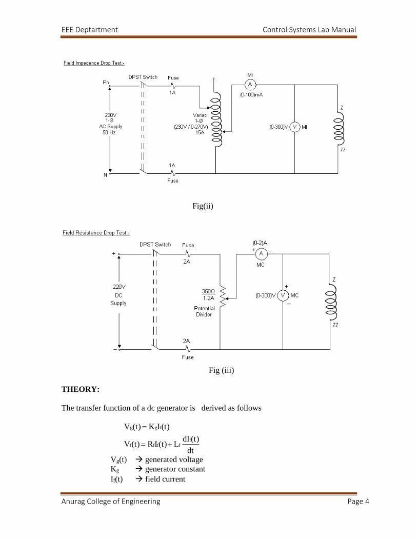
Fig(ii)
Fig (iii)
THEORY:
The transfer function of a dc generator is derived as follows
dt
(t)dIL(t)IR(t)V
(t)IK(t)V
fffff
fgg
Vg(t) generated voltage
Kg generator constant
If(t) field current
EEE Deptartment Control Systems Lab Manual
Anurag College of Engineering Page 5
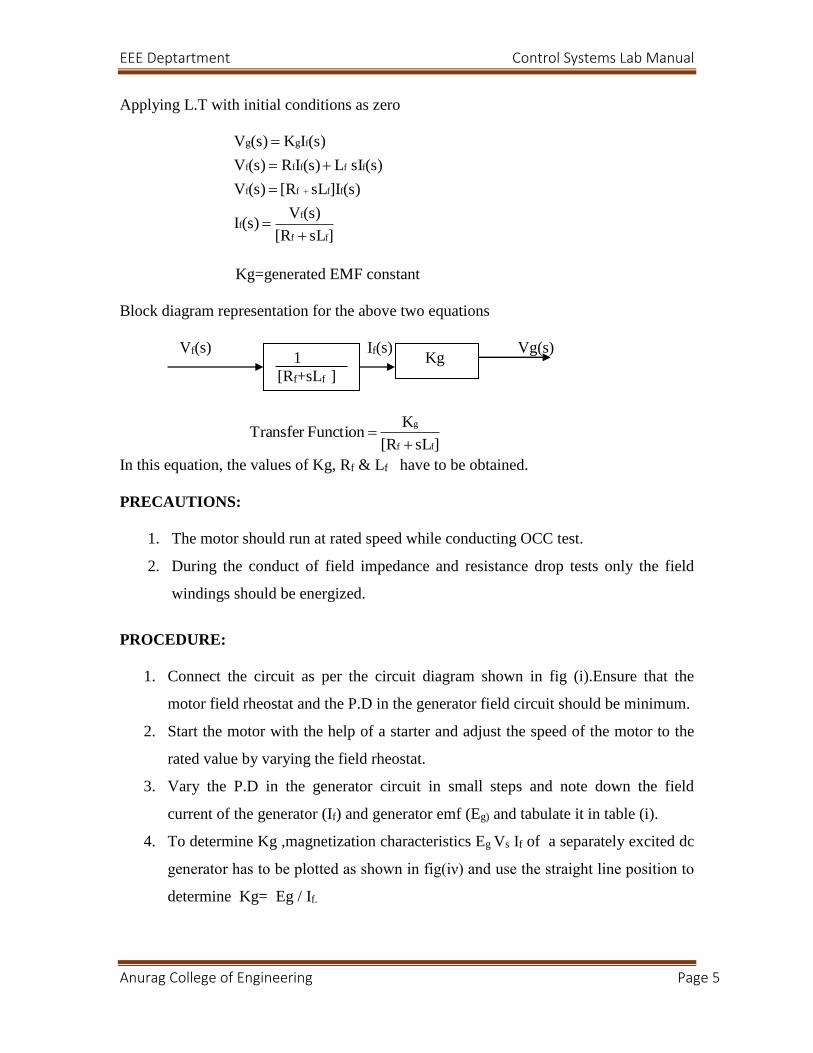
Applying L.T with initial conditions as zero
]sL[R
(s)V(s)I
(s)]IsL[R(s)V
(s)sI L(s)IR(s)V
(s)IK(s)V
ff
ff
ffff
fffff
fgg
Kg=generated EMF constant
Block diagram representation for the above two equations
Vf(s) If(s) Vg(s)
]sL[R
KFunctionTransfer
ff
g
In this equation, the values of Kg, Rf & Lf have to be obtained.
PRECAUTIONS:
1. The motor should run at rated speed while conducting OCC test.
2. During the conduct of field impedance and resistance drop tests only the field
windings should be energized.
PROCEDURE:
1. Connect the circuit as per the circuit diagram shown in fig (i).Ensure that the
motor field rheostat and the P.D in the generator field circuit should be minimum.
2. Start the motor with the help of a starter and adjust the speed of the motor to the
rated value by varying the field rheostat.
3. Vary the P.D in the generator circuit in small steps and note down the field
current of the generator (If) and generator emf (Eg) and tabulate it in table (i).
4. To determine Kg ,magnetization characteristics Eg Vs If of a separately excited dc
generator has to be plotted as shown in fig(iν) and use the straight line position to
determine Kg= Eg / If.
Kg
1
[Rf+sLf ]
EEE Deptartment Control Systems Lab Manual
Anurag College of Engineering Page 6
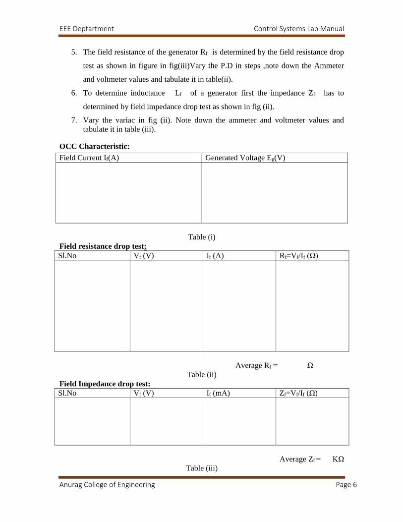
5. The field resistance of the generator Rf is determined by the field resistance drop
test as shown in figure in fig(iii)Vary the P.D in steps ,note down the Ammeter
and voltmeter values and tabulate it in table(ii).
6. To determine inductance Lf of a generator first the impedance Zf has to
determined by field impedance drop test as shown in fig (ii).
7. Vary the variac in fig (ii). Note down the ammeter and voltmeter values and
tabulate it in table (iii).
OCC Characteristic:
Field Current If(A) Generated Voltage Eg(V)
Table (i)
Field resistance drop test:
Sl.No Vf (V) If (A) Rf=Vf/If (Ω)
Average Rf = Ω
Table (ii)
Field Impedance drop test:
Sl.No Vf (V) If (mA) Zf=Vf/If (Ω)
Average Zf = KΩ
Table (iii)

EEE Deptartment Control Systems Lab Manual
Anurag College of Engineering Page 7
CALCULATIONS
Field resistance Rf =1.2* Rf avg Ω
Impedance Zf = KΩ
][(s)V
)(VT.F
FunctionTransfer
K
graph From
f2
X
]R[ZX
f
g
g
f
212
f
2
ff
ff
g
f
g
f
sLR
Ks
I
E
L
MODEL GRAPH:
Fig (iν)
RESULT:
The transfer function of dc generator was determined by conducting OCC test on the
given dc generator and the T.F of the system is found to be
f
Lf
RgK
T.F

EEE Deptartment Control Systems Lab Manual
Anurag College of Engineering Page 8
2. Magnetic Amplifier AIM:
To Study the control characteristics of a Magnetic Amplifier
APPARATUS:
1. Magnetic Amplifier having laminated core.
Ammeters D.C (0-100ma), Ammeters A.C (0-500ma) are arranged in unit itself
2. Patch cards
3. Low Bulb
THEORY:
1. Magnetic amplifier is a device consisting of saturable reactors, rectifiers and
conventional transformers, used to secure control or amplication.
2. The load current in magnetic amplifier is cotrolled by a D.C.magnetizing current.
3. A large current value is controlled by a small current value; hence such type of
circuits is termed as current amplifiers.
4. To control the load current, a saturable reactor is used.The reactance of the reactor
depends upon magnetic coupling and magnetism induced depends upon the
D.C.control current.
5. The load current is controlled by using magnetic property and hence the term
magnetic amplifier.
6. The most common basic saturable reactor which is used in magnetic amplifier
circuits consists of a three legged closed laminated core with coils wound on each
leg.
7. The coils wound on central limb are called as control winding and coils wound on
outer limbs are called as load winding.
8. Due to D.C.current in the control winding, the degree of magnetization in the core
is changed.
9. Hence the flux density changes, i.e.reactance of the core by changing the
D.C.current in the control winding.
10. If the load winding is connected in series with the load, one can control the
current in the load by changing reactance of the coil with the help of D.C.control
current.
EEE Deptartment Control Systems Lab Manual
Anurag College of Engineering Page 9
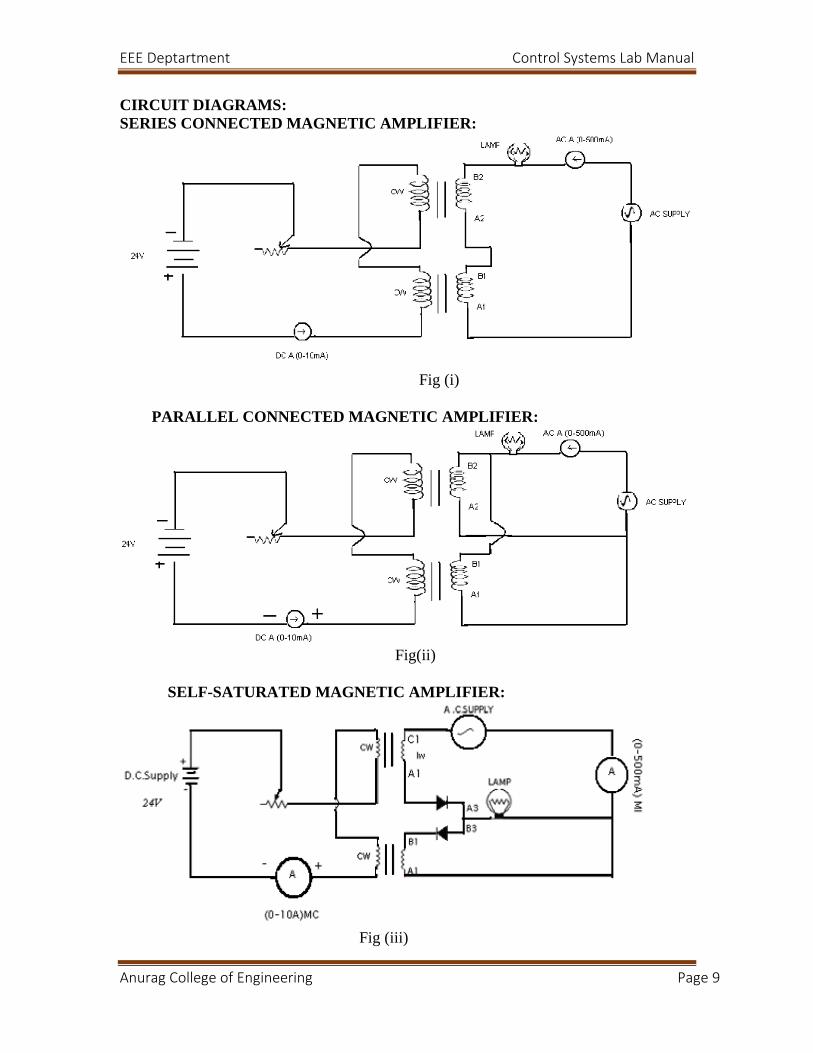
CIRCUIT DIAGRAMS:
SERIES CONNECTED MAGNETIC AMPLIFIER:
Fig (i)
PARALLEL CONNECTED MAGNETIC AMPLIFIER:
Fig(ii)
SELF-SATURATED MAGNETIC AMPLIFIER:
Fig (iii)

EEE Deptartment Control Systems Lab Manual
Anurag College of Engineering Page 10
PROCEDURE:
SERIES CONNECTION:
1. Connected the circuit as per the circuit diagram shown in fig (i).
2. Keep the slide switch on ‘D’ position which will be indicated by an indicator after
circuit is switched on
3. Keep control switch knob at its extreme position which ensure zero control
current at starting.
4. With the help of patch cards connect the following terminals on the front panels
of the unit
a) Connect AC to A1
b) Connect B1 to B2
c) Connect B2 to L
5. Connect a 100w fluorescent lamp in the holder and switch on the unit.
6. Now gradually increase the control current by rotating control current setting
knob clockwise in steps and note down control current and corresponding load
current and tabulate it in table (i).
7. Plot the graph of load current Vs control current.
B.PARALLEL CONNECTION:
1. Connect the circuit as per the circuit diagram shown in fig (ii)
2. Keep slide switch in position ‘D’ which will be indicated by an indicator after unit
is switched on.
3. Keep control current setting knob at its extreme left position which ensures zero
control current at starting.
4. With the help of plug in links, connect following terminals on the front panel of
the unit.
a) Connect AC to A1
b) Connect A1 to A2
c) Connect B1 to B2
d) Connect B2 to L

EEE Deptartment Control Systems Lab Manual
Anurag College of Engineering Page 11
5. Connect 100 watt fluorescent lamp in the holder provide for this purpose and
switch on the unit
6. Now gradually increase control current by rotating control current setting knob
clockwise in steps and note down control current and corresponding load current
and tabulate it in table (ii).
7. Plot the graph of load current vs control current.
C. SELF SATURATED CONNECTION:
1. Connect the circuit as per the circuit diagram shown in fig(iii).
2. Keep slide switch in position ‘E’ which will be indicated by an indicator, after
unit is switched on.
3. Keep control switch knob at its extreme position which ensures zero control
current at staring.
4. With the help of patch cards connect the following terminals on the front panel of
the unit.
a) Connect Ac to C1
b) Connect A3 to B3
c) Connect B3 to L
5. Connect a 100W fluorescent lamp in the holder provide for this purpose and witch
on the unit.
6. Now gradually increase control current by rotating control current setting knob
clockwise in steps and note down control current and corresponding load current
and tabulate it in table (iii).
7. Plot the graph of load current Vs control current.
PRECAUTIONS:
1. For series and parallel connections of the magnetic amplifier the switch should be in D
mode.
2. For self saturation connection the switch is thrown to position E.

EEE Deptartment Control Systems Lab Manual
Anurag College of Engineering Page 12
TABULAR COLUMNS:
SERIES CONNECTION:
Sl.No Ic (mA) IL (mA)
Table (i)
PARALLEL CONNECTION:
Sl.No Ic (mA) IL (mA)
Table (ii)
SELF SATURATION CONNECTION:
Sl.No Ic (mA) IL (mA)
Table (iii)
MODEL GRAPHS:
SERIES CONNECTION:
EEE Deptartment Control Systems Lab Manual
Anurag College of Engineering Page 13
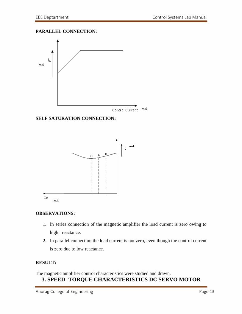
PARALLEL CONNECTION:
SELF SATURATION CONNECTION:
OBSERVATIONS:
1. In series connection of the magnetic amplifier the load current is zero owing to
high reactance.
2. In parallel connection the load current is not zero, even though the control current
is zero due to low reactance.
RESULT:
The magnetic amplifier control characteristics were studied and drawn.
3. SPEED- TORQUE CHARACTERISTICS DC SERVO MOTOR
EEE Deptartment Control Systems Lab Manual
Anurag College of Engineering Page 14
AIM:
To draw the speed - torque characteristics of a dc-servomotor.
APPARATUS:
Dc Servo Motor
Multimeter (Or) Voltmeter
Connecting Wires
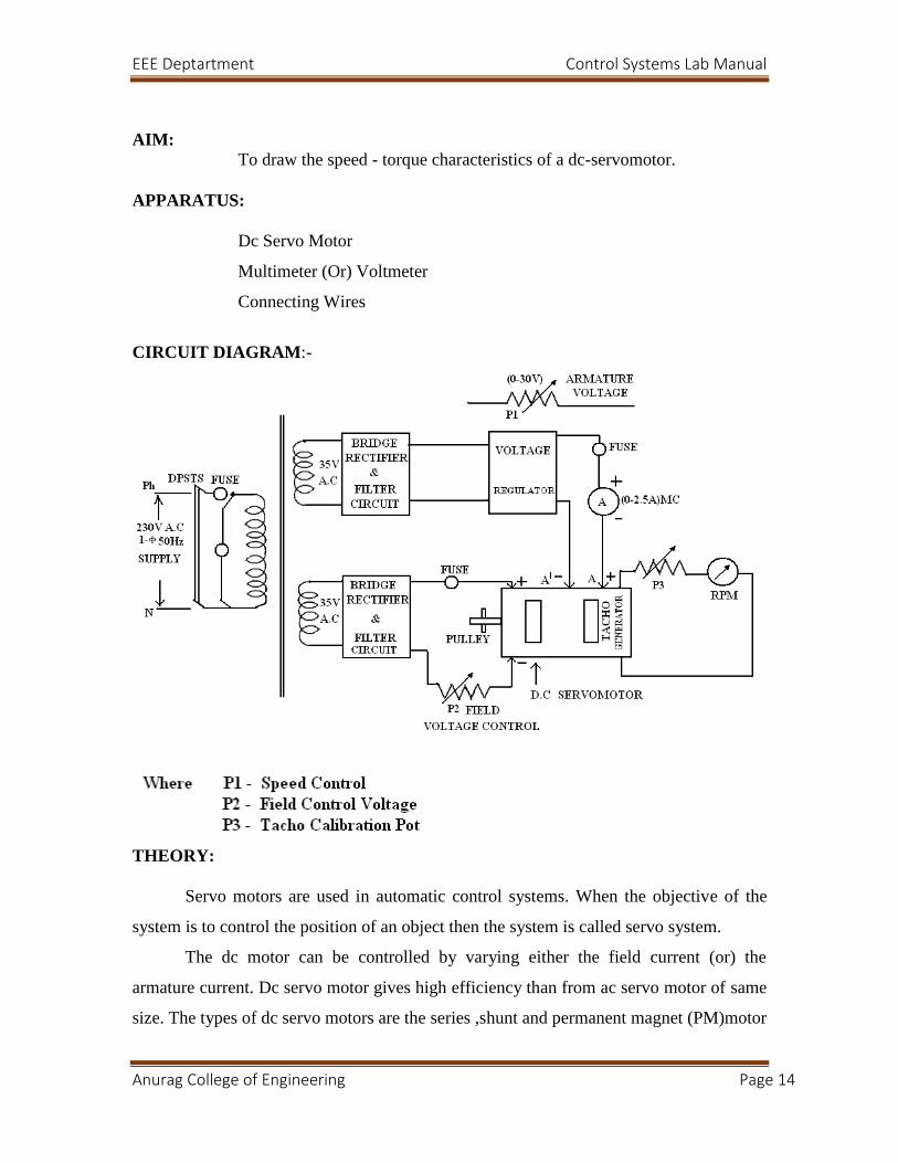
CIRCUIT DIAGRAM:-
THEORY:
Servo motors are used in automatic control systems. When the objective of the
system is to control the position of an object then the system is called servo system.
The dc motor can be controlled by varying either the field current (or) the
armature current. Dc servo motor gives high efficiency than from ac servo motor of same
size. The types of dc servo motors are the series ,shunt and permanent magnet (PM)motor
EEE Deptartment Control Systems Lab Manual
Anurag College of Engineering Page 15
.the ease of controllable speed along with linear torque speed control curve makes the PM
motor ideal for servo mechanism applications
PRECAUTIONS:
1. The speed control knob is always in the most anti clock wise position before
switching on the position.
2. In order to increase the armature voltage, rotate the knob in the clock wise
direction in a gentle fashion.
3. In order to increase the load on the motor, adjust the knob K in a gentle fashion.
PROCEDURE:
1. Adjust T1 to 40gm with the help of knob K.
2. Ensure the pot P1 is in maximum position, switch on the supply.
3. Connect the voltmeters across the terminals of armature and field.
4. Adjust P1 so that Va =10v and P2 such that V f =20v.
5. Note down T1and T2 and speed values in tabular column.
6. Keeping Va=10v, adjust T1 up to 150gm in steps of readings.
7. Now for Va =15, 20, 25 and 30v repeat step 6.
8. From the table plot the speed –torque characteristics.
9. Repeat the above step for various values of Vf by controlling P2 .
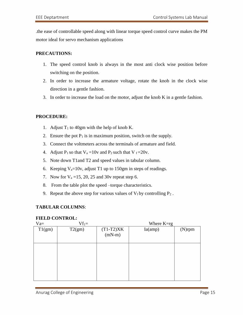
TABULAR COLUMNS:
FIELD CONTROL: Va= Vf1= Where K=rg
T1(gm)
T2(gm) (T1-T2)XK
(mN-m)
Ia(amp) (N)rpm

EEE Deptartment Control Systems Lab Manual
Anurag College of Engineering Page 16
Va= Vf2=
T1(gm) T2(gm) (T1-
T2)K(mN-m)
Ia(amp) N(rpm)
Va= Vf3=
T1(gm) T2(gm) (T1-T2)K(mN-
m)
Ia(amp) N(rpm)
ARMATURE CONTROL:
Va1= Vf=
T1(gm) T2(gm) (T1-T2)K(mN-m) Ia(amp) N(rpm)
Va2= Vf=
T1(gm) T2(gm) (T1-T2)K(mN-m) Ia(amp) N(rpm)
Va3= Vf=
T1(gm) T2(gm) (T1-T2)K(mN-m) Ia(amp) N(rpm)
EEE Deptartment Control Systems Lab Manual
Anurag College of Engineering Page 17
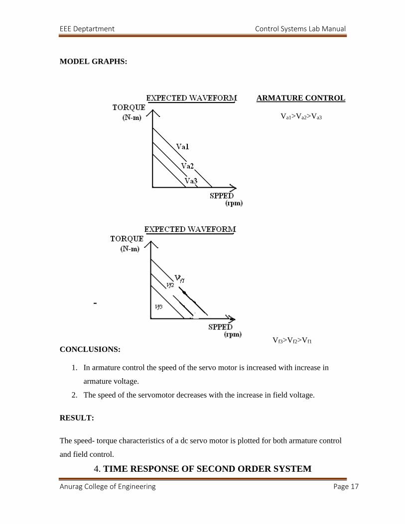
MODEL GRAPHS:
ARMATURE CONTROL
Va1>Va2>Va3
Vf3>Vf2>Vf1
CONCLUSIONS:
1. In armature control the speed of the servo motor is increased with increase in
armature voltage.
2. The speed of the servomotor decreases with the increase in field voltage.
RESULT:
The speed- torque characteristics of a dc servo motor is plotted for both armature control
and field control.
4. TIME RESPONSE OF SECOND ORDER SYSTEM

EEE Deptartment Control Systems Lab Manual
Anurag College of Engineering Page 18
AIM:
1. To obtain the time response of second order system
2. To determine time domain specifications.
APPARATUS:
Decade resistance box
Decade inductance box
Decade capacitance box
Function generator
CRO probes
Connecting wires.
.
CIRCUIT DIAGRAM:
Fig (i)
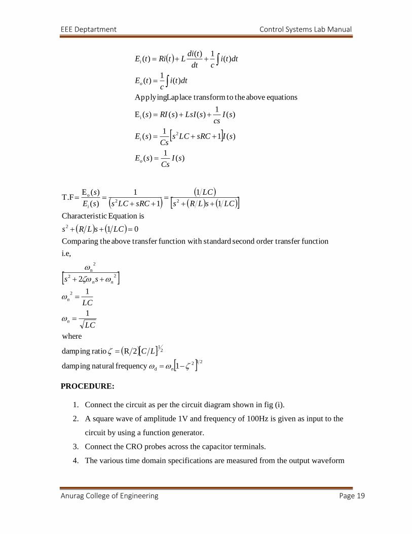
THEORY:
The time response of second order system is defined as the response of the system as the
function of time. Apply the KVL to the circuit,
EEE Deptartment Control Systems Lab Manual
Anurag College of Engineering Page 19
)(1
)(
)(11
)(
)(1
)()()(E
equations above the to transformLaplace Applying
)(1
)(
)(1)(
)(
2
i
sICs
sE
sIsRCLCsCs
sE
sIcs
sLsIsRIs
dttic
tE
dtticdt
tdiLtRitE
o
i
o
i
212
d
21
2
22
2
n
2
22
o
1frequency natural damping
2R ratio damping
where
1
1
2
i.e,
functionsfer order tran second standardith function w transfer above theComparing
01
isEquation sticCharacteri
1
1
1
1
)(
)(E T.F
n
n
n
nn
i
LC
LC
LC
ss
LCsLRs
LCsLRs
LC
sRCLCssE
s
PROCEDURE:
1. Connect the circuit as per the circuit diagram shown in fig (i).
2. A square wave of amplitude 1V and frequency of 100Hz is given as input to the
circuit by using a function generator.
3. Connect the CRO probes across the capacitor terminals.
4. The various time domain specifications are measured from the output waveform
EEE Deptartment Control Systems Lab Manual
Anurag College of Engineering Page 20
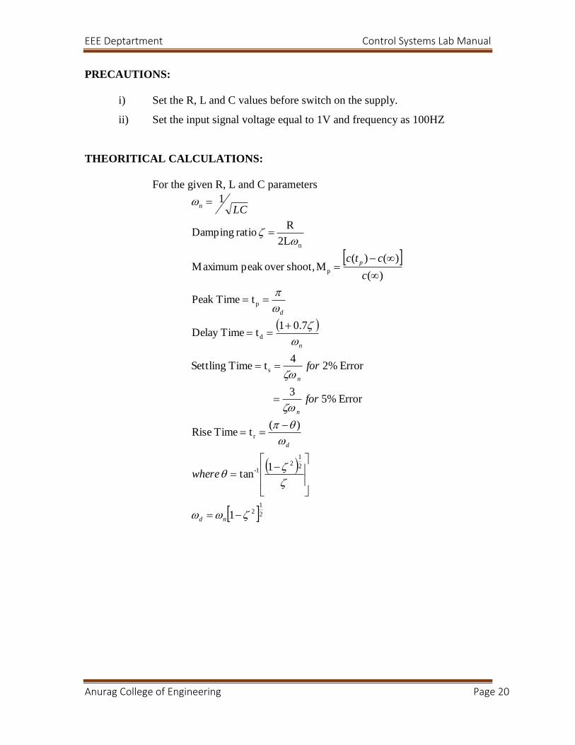
PRECAUTIONS:
i) Set the R, L and C values before switch on the supply.
ii) Set the input signal voltage equal to 1V and frequency as 100HZ
THEORITICAL CALCULATIONS:
For the given R, L and C parameters
21
2
2
12
1-
r
s
d
p
p
n
1
1tan
)(t Time Rise
Error 5% 3
Error 2% 4
tTime Settling
7.01t TimeDelay
tTimePeak
)(
)()(M shoot,over peak Maximum
2L
R ratio Damping
1
nd
d
n
n
n
d
p
n
where
for
for
c
ctc
LC

EEE Deptartment Control Systems Lab Manual
Anurag College of Engineering Page 21
MODEL GRAPH:
PRACTICAL OBSERVATIONS:
Max % peak over shoot, %Mp =
Delay time, td =
Rise time, tr = Peak time, tp =
Settling time, ts =
TABULAR COLUMN:
Time domain specifications Practical observations Theoretical
calculations
Max % peak over shoot, %Mp
Delay time, td
Rise time, tr
Peak time, tp
Settling time, ts

EEE Deptartment Control Systems Lab Manual
Anurag College of Engineering Page 22
OBSERVATIONS:
1. In the output response tolerance errors can not be observable.
2. Settling time in the output response can be observed only at the 5%
tolerance.
RESULT:
The response of second order system was obtained and time domain specifications were
obtained from the response.
The time domain specifications are :
% Mp=
td =
tr =
tp =
ts =
5. LAG COMPENSATOR
AIM:
To study the electrical lag compensator network experimentally and to draw bode plots
for improvement of steady state and transient behavior of system.
APPARATUS:
1. CRO with 2 channels
2. frequency generator to supply a variable frequency sinusoidal source
3. lag compensator kit (R1=20kΩ,R2=25kΩ& C=0.2nf)
4. 1:1 CRO probes -2 Nos
CIRCUIT DIAGRAM:

EEE Deptartment Control Systems Lab Manual
Anurag College of Engineering Page 23
Fig (i)
THEORY:
Some kind of corrective subsystems introduce in a system to force the plant to meet the
desired specifications. These sub systems are known as compensators. Desired
specifications mean transient response and steady state error. In general, there are two
situations in which compensator are required to stabilize it as well as to achieve a specific
performance. In the 2nd case the system is stable. But the compensation is required to
obtain the desired performance. The lag compensation is required to improve the steady
state behavior of the system of a system while nearly preserving its transient response.
THEORITICAL CALCULATIONS:
The general form of the T.F of lag compensator is
1 1
s
1s
)(
c
c
c
cc
p
Z
ps
zssG
From the electrical lag- network
EEE Deptartment Control Systems Lab Manual
Anurag College of Engineering Page 24
s
s
C
RRs
s
CRRRRs
CRs
R
CRRsCRR
CRsC
sCRR
sCR
sE
sE
sCRR
sCR
sE
sE
i
i
o
1
1
R
1)(R 1
11
1
1
)(R
R
1)(1)(
1R
1)(
1
)(
)(
1
1
)(
)(
2
221
2212
2
21
2
2121
22
21
20
21
2
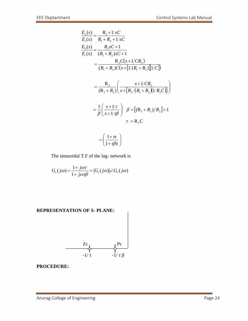
The sinusoidal T.F of the lag- network is
)()(1
1)(
jGjG
j
jjG ccc
REPRESENTATION OF S- PLANE:
Zc Pc
-1/ τ -1/ τ β
PROCEDURE:
EEE Deptartment Control Systems Lab Manual
Anurag College of Engineering Page 25
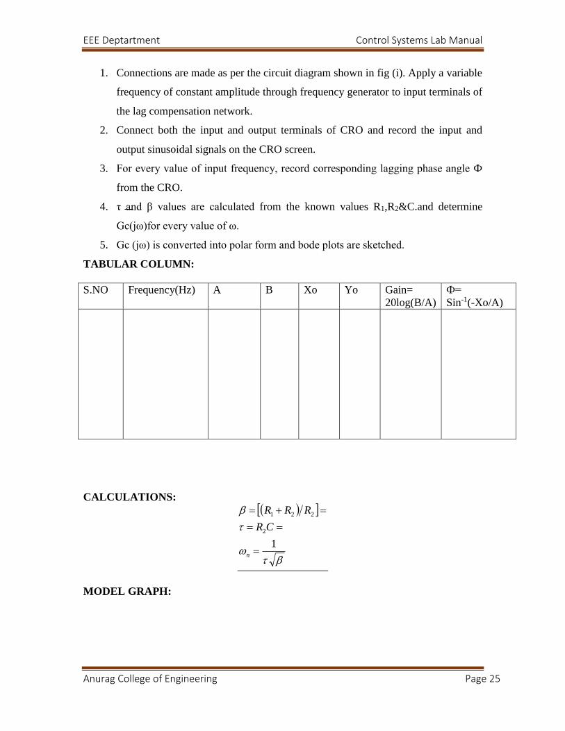
1. Connections are made as per the circuit diagram shown in fig (i). Apply a variable
frequency of constant amplitude through frequency generator to input terminals of
the lag compensation network.
2. Connect both the input and output terminals of CRO and record the input and
output sinusoidal signals on the CRO screen.
3. For every value of input frequency, record corresponding lagging phase angle Ф
from the CRO.
4. τ and β values are calculated from the known values R1,R2&C.and determine
Gc(jω)for every value of ω.
5. Gc (jω) is converted into polar form and bode plots are sketched.
TABULAR COLUMN:
S.NO Frequency(Hz) A B Xo Yo Gain=
20log(B/A)
Ф=
Sin-1(-Xo/A)
CALCULATIONS:
1
2
221
n
CR
RRR
MODEL GRAPH:
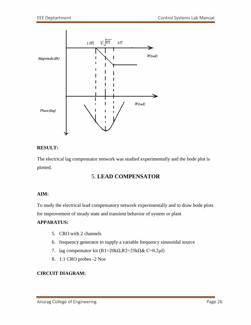
EEE Deptartment Control Systems Lab Manual
Anurag College of Engineering Page 26
RESULT:
The electrical lag compensator network was studied experimentally and the bode plot is
plotted.
5. LEAD COMPENSATOR
AIM:
To study the electrical lead compensatory network experimentally and to draw bode plots
for improvement of steady state and transient behavior of system or plant
APPARATUS:
5. CRO with 2 channels
6. frequency generator to supply a variable frequency sinusoidal source
7. lag compensator kit (R1=20kΩ,R2=25kΩ& C=0.2μf)
8. 1:1 CRO probes -2 Nos
CIRCUIT DIAGRAM:

EEE Deptartment Control Systems Lab Manual
Anurag College of Engineering Page 27
Fig (ii)
THEORY:
A lead compensator speeds up the transient response and increases the margin of stability
of system .it also helps to increase the system error constant through to a limited extent.
THEORITICAL CALCULATIONS:
The general form of the T.F of lag compensator is

EEE Deptartment Control Systems Lab Manual
Anurag College of Engineering Page 28
)()(1
1)(G
isnetwork lag a offunction transfer sinusoidal The
1
1
,1,1
1
1
1
1R
1R
)1(1)(
)(E
network-lead Electrical the
1,1
1
)(
c
1212
1221
1
212121
121
1212
12
112
20
jGjGj
jj
s
s
CRRRRs
s
CRRRRs
CRs
CRRRRsCRR
CRsCR
RCsRRR
CsR
CsRCsRR
R
sE
s
For
PZs
s
Ps
ZssG
cc
i
cc
c
cc
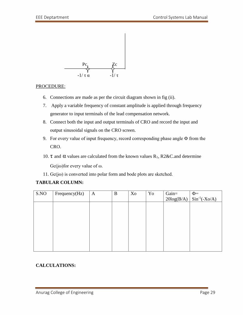
REPRESENTATION OF S- PLANE:
EEE Deptartment Control Systems Lab Manual
Anurag College of Engineering Page 29
Pc Zc
-1/ τ α -1/ τ
PROCEDURE:
6. Connections are made as per the circuit diagram shown in fig (ii).
7. Apply a variable frequency of constant amplitude is applied through frequency
generator to input terminals of the lead compensation network.
8. Connect both the input and output terminals of CRO and record the input and
output sinusoidal signals on the CRO screen.
9. For every value of input frequency, record corresponding phase angle Ф from the
CRO.
10. τ and α values are calculated from the known values R1, R2&C.and determine
Gc(jω)for every value of ω.
11. Gc(jω) is converted into polar form and bode plots are sketched.
TABULAR COLUMN:
S.NO Frequency(Hz) A B Xo Yo Gain=
20log(B/A)
Ф=
Sin-1(-Xo/A)
CALCULATIONS:

EEE Deptartment Control Systems Lab Manual
Anurag College of Engineering Page 30
1
1
212
n
CR
RRR
MODEL GRAPH:
RESULT:
The electrical lead compensator network was studied experimentally and the bode plots
are plotted.
6. SIMULATION OF TRANSFER FUNCTION USING OP-AMPS
AIM:
To simulate the transfer function using Op-Amps, by using the circuits Integrator,
Non inverting amplifier and summing amplifier.
APPARATUS:
Op- Amps IC -741 -3 NO’S
Capacitor 0.1μF -1 No.
Resistor 10 KΩ -5 No’s
EEE Deptartment Control Systems Lab Manual
Anurag College of Engineering Page 31
2 KΩ- 2 No.’s
100KΩ- 1 No.
Function Generator, CRO & probes, connecting wires.
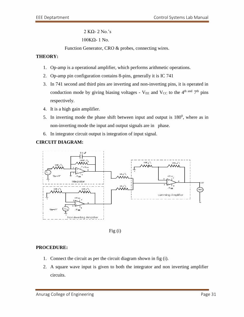
THEORY:
1. Op-amp is a operational amplifier, which performs arithmetic operations.
2. Op-amp pin configuration contains 8-pins, generally it is IC 741
3. In 741 second and third pins are inverting and non-inverting pins, it is operated in
conduction mode by giving biasing voltages - VEE and VCC to the 4th and 7th pins
respectively.
4. It is a high gain amplifier.
5. In inverting mode the phase shift between input and output is 1800, where as in
non-inverting mode the input and output signals are in phase.
6. In integrator circuit output is integration of input signal.
CIRCUIT DIAGRAM:
Fig (i)
PROCEDURE:
1. Connect the circuit as per the circuit diagram shown in fig (i).
2. A square wave input is given to both the integrator and non inverting amplifier
circuits.

EEE Deptartment Control Systems Lab Manual
Anurag College of Engineering Page 32
3. +Vcc and –Vee are applied as +10v and -10v at 7 and 4 pins respectively for
every circuit shown in the circuit diagram.
4. Individual out puts V01 and V02 of integrator and non inverting amplifier are
summed by using a summing amplifier which is shown in figure.
5. The output waveform of integrator, non-inverting amplifier and summing
amplifier are observed and plotted on the graph
THEORITICAL CALCULATIONS:-.
For the integrator circuit,
)01.1(
10
)1(1
R
R-
1
f
1sCsR
K
CsRT
ff
For the Non- inverting amplifier,
.01s)(1
10-2
TT
amplifier summingFor
21
21
12
T
RRT f
MODEL GRAPH:

EEE Deptartment Control Systems Lab Manual
Anurag College of Engineering Page 33
RESULT:
The transfer function of the op-amp was simulated.
7. STATE SPACE TO TRANSFER FUNCTION
USING MATLAB
AIM:
To determine the transfer function for the given state space representation.
EEE Deptartment Control Systems Lab Manual
Anurag College of Engineering Page 34
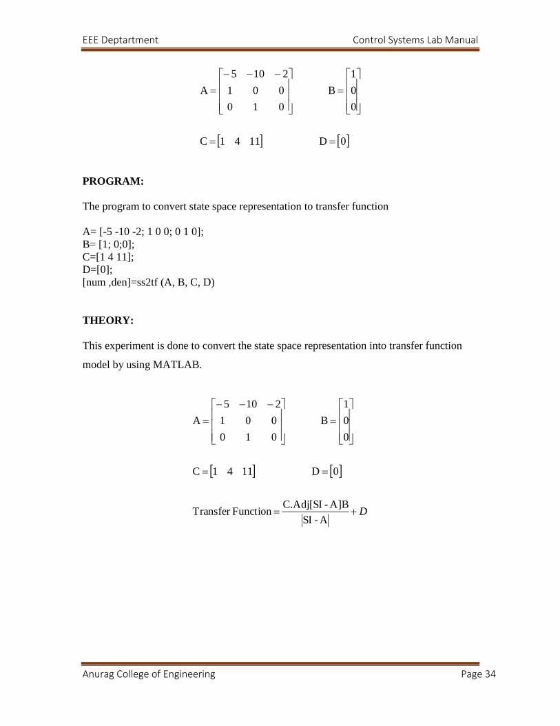
0D 1141C
0
0
1
B
010
001
2105
A
PROGRAM:
The program to convert state space representation to transfer function
A= [-5 -10 -2; 1 0 0; 0 1 0];
B= [1; 0;0];
C=[1 4 11];
D=[0];
[num ,den]=ss2tf (A, B, C, D)
THEORY:
This experiment is done to convert the state space representation into transfer function
model by using MATLAB.
D
A-SI
A]B-C.Adj[SI Function Transfer
0D 1141C
0
0
1
B
010
001
2105
A
EEE Deptartment Control Systems Lab Manual
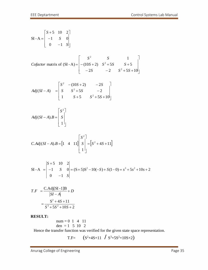
Anurag College of Engineering Page 35
2105
114S
1]B-C.Adj[SI .
2105)01()(105)S(S
10
01
2105
A -SI
114
1
1141).(.
1
).(
10551
25
2)210(
)(
10522
55)210(
1
A)-(SI ofmatrix
10
01
2105
A-SI
23
2
232
2
2
2
2
2
2
2
2
2
SSS
S
DASI
FT
sssSS
S
S
S
SSS
S
BASIAdjC
S
S
BASIAdj
SSS
SSS
SSS
ASIAdj
SSS
SSSS
SS
Cofactor
S
S
S
RESULT:
num = 0 1 4 11
den = 1 5 10 2
Hence the transfer function was verified for the given state space representation.
T.F= (S2+4S+11 / S3+5S2+10S+2)

EEE Deptartment Control Systems Lab Manual
Anurag College of Engineering Page 36
8. PLOTING OF ROOT LOCUS
AIM:
To obtain root locus plot for a given transfer function 1/ (s2-4s+8) by using MATLAB.
PROGRAM: num= [1];
den= [1 -4 8];
rlocus (tf (num, den))
THEORY:
The root locus technique is used for stability analysis. Using the root locus
the range of values of K, for a stable system can be determined. It is also easier to study
the relative stability of the system from the knowledge of location of closed loop poles.
The root locus can be plotted in S-plane by verifying system parameters over the
complete range of values. The roots corresponding to a particular value of the system
parameter can then be located on the locus ors the value of the parameter for a desired
root locus can be determined from root locus.
PROCEDURE:
From the command window open new .M file. Write a program and
save it on to the desktop and come back to the command window. Now type .M file
name and observe the root locus.
THEORETICAL CALCULATIONS:
Given transfer function = 84
12 ss
Characteristic equation is 0842 ss
The roots are (2-j2) & (2+j2)

EEE Deptartment Control Systems Lab Manual
Anurag College of Engineering Page 37
MODEL GRAPH:
RESULT:
The root locus plot for a given transfer function was verified in MATLAB.
9. STATE SPACE REPRESENTATION OF TRANSFER FUNCTION
USING MATLAB
AIM:
To determine the state space representation for the given transfer function
PROGRAM:
The program to convert transfer function in to state space representation
num = [a b c];
den = [1 p q r];
[A B C D] = tf2ss (num, den)
THEORY:
This experiment is done to convert the state space representation into transfer function
model by using MATLAB.
EEE Deptartment Control Systems Lab Manual
Anurag College of Engineering Page 38
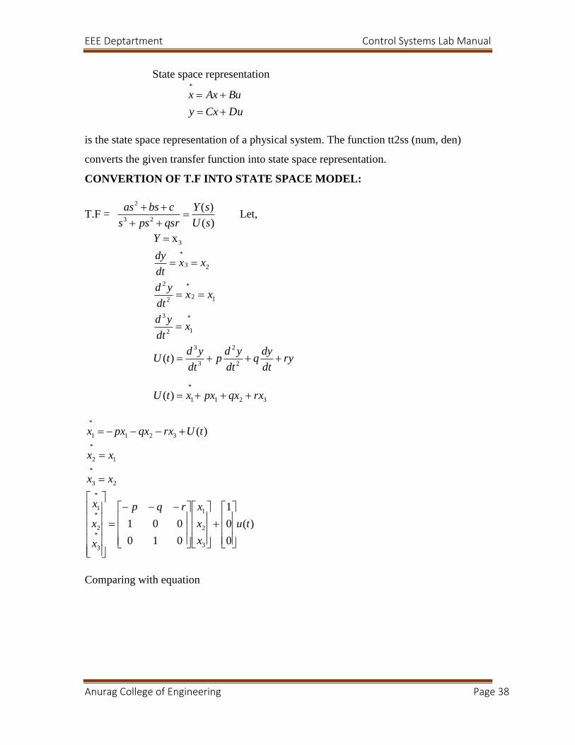
State space representation
DuCxy
BuAxx
*
is the state space representation of a physical system. The function tt2ss (num, den)
converts the given transfer function into state space representation.
CONVERTION OF T.F INTO STATE SPACE MODEL:
T.F = )(
)(23
2
sU
sY
qsrpss
cbsas
Let,
321
*
1
2
2
3
3
*
12
3
12
*
2
2
23
*
3
)(
)(
x
rxqxpxxtU
rydt
dyq
dt
ydp
dt
ydtU
xdt
yd
xxdt
yd
xxdt
dy
Y
)(
0
0
1
010
001
)(
3
2
1
*
3
*
2
*
1
2
*
3
1
*
2
321
*
1
tu
x
x
xrqp
x
x
x
xx
xx
tUrxqxpxx
Comparing with equation

EEE Deptartment Control Systems Lab Manual
Anurag College of Engineering Page 39
)(]0[
)(
)(
)(
0
0
1
B
010
001
3
2
1
321
2
2
2
*
tU
x
x
x
cbaY
cxbxaxtY
cydt
dyb
dt
ydatY
cbsastY
rqp
A
then
BuAxx
Comparing with
Y=CX+DU
[0]D cbaC
There fore
[0]D
0
0
1
B
010
001
cbaC
rqp
A
RESULT:
[0]D
0
0
1
B
010
001
cbaC
rqp
A
The state space representation for the given transfer function was verified using
MATLAB


