Control Systems - Chibum Lee | personal blog · Chibum Lee -Seoultech Control Systems...
33
Transcript of Control Systems - Chibum Lee | personal blog · Chibum Lee -Seoultech Control Systems...

Control SystemsChibum Lee -Seoultech
Outline
Dominant pole design
Symmetric root locus
Control SystemsChibum Lee -Seoultech
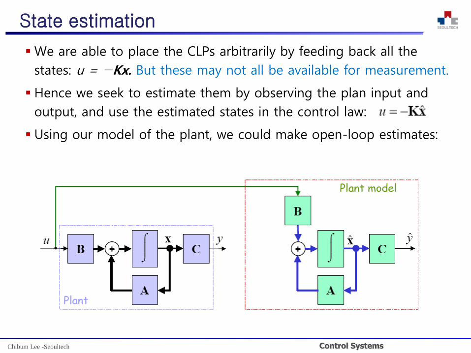
State estimation
We are able to place the CLPs arbitrarily by feeding back all the
states: u = −Kx. But these may not all be available for measurement.
Hence we seek to estimate them by observing the plan input and
output, and use the estimated states in the control law:
Using our model of the plant, we could make open-loop estimates:

Control SystemsChibum Lee -Seoultech
State estimation
However,
• our model may not be precise
• we don't know the plant's initial conditions
• the plant may be subject to unmodelled disturbances
• hence the estimated state is likely to diverge from the actual state
We therefore introduce feedback to try to get the estimated output
ŷ to track the measured output y

Control SystemsChibum Lee -Seoultech
State estimation
is a vector of feedback gains
Thus, we form our estimates from
equations to beimplemented inestimator

Control SystemsChibum Lee -Seoultech
Estimator dynamics
Given the plant input u and measured output y, the state estimate
evolves according to:
Our plant model is
Subtracting, and using the output equation, gives:
Denote the error in the state estimate by
Then the error dynamics are:
That is, given the assumptions of a perfect plant model, and no
disturbances, this suggests that the estimation error can be made
to go to zero in a stable and rapid manner by a suitable choice of L

Control SystemsChibum Lee -Seoultech
Estimator dynamics
The estimated states should then continue to track the plant states
with zero error
In reality there will be estimation errors:
• plant disturbances
• model imperfections
These errors can be kept small if the eigenvalues of the error
system are well damped and relatively fast
compared with the closed-loop plant dynamics
Characteristic polynomial for error dynamics:
Desired characteristic polynomial:
Provided system is observable, we can solve for L so that aL(s) =
αe(s), using the same techniques as for K

Control SystemsChibum Lee -Seoultech
Benefit of observer canonical form
The solution for the estimator gain matrix L is trivial if the
equations are in observer canonical form
The system matrix for the error equation is then:
This is still in observer c.f., and has the char. poly
Compare with desired char. poly:
Hence, by inspection: L1 = β1 – a1, L2 = β2 – a2, L3 = β3 – a3

Control SystemsChibum Lee -Seoultech
Ackermann's formula
Again, Ackermann's formula can be used to effectively implement
the process of:
• transformation of an observable system to observer canonical form
• design of estimator gains by inspection
• transformation back to original states
c.f.
MATLAB: Specify desired estimator poles, dep
• L = acker(A’, C’, dep)’
• L = place(A’, C’, dep)’

Control SystemsChibum Lee -Seoultech
Relationships between canonical forms: Duality
Observercanonicalform
Controllercanonicalform
Observabilitycanonicalform
Controllabilitycanonicalform

Control SystemsChibum Lee -Seoultech
Regulator with estimated states
Plant:
Control law:
Estimator:

Control SystemsChibum Lee -Seoultech
State equations for closed-loop system
Plant:
Estimator:
Control law:
Combining these equations:
Thus the closed-loop state equations are:
Control SystemsChibum Lee -Seoultech
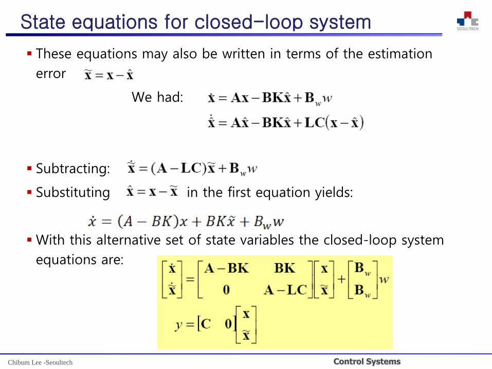
State equations for closed-loop system
These equations may also be written in terms of the estimation
error
We had:
Subtracting:
Substituting in the first equation yields:
With this alternative set of state variables the closed-loop system
equations are:

Control SystemsChibum Lee -Seoultech
State equations for closed-loop system
The closed-loop characteristic polynomial is thus:
which is block triangular. Hence:
Thus, the poles of the CL system consist of the poles obtained by
full state feedback through K, together with the estimator poles
determined by the selection of L
That is, the control law and the estimator can be designed
independently of each other Separation Principle

Control SystemsChibum Lee -Seoultech
Ex: regulation of water level in two-tank system
The system can be described
For

Control SystemsChibum Lee -Seoultech
Ex: regulation of water level in two-tank system
Specs: Required closed-loop time constants are 1 = 0.2 s, 2 = 0.05
s; i.e., desired CL char. poly is
Control law: Demonstrate Ackermann's formula:

Control SystemsChibum Lee -Seoultech
Ex: regulation of water level in two-tank system
Estimator: Try estim. poles = 2 x controller poles;
• i.e., desired CL char. poly is α = (s +10)(s + 40) = s2 + 50s + 400
Demonstrate Ackermann's formula:

Control SystemsChibum Lee -Seoultech
Ex: regulation of water level in two-tank system
Complete system
• Equivalent feedback compensator:
• Transfer function for compensator:

Control SystemsChibum Lee -Seoultech
Example 7.25

Control SystemsChibum Lee -Seoultech

Control SystemsChibum Lee -Seoultech
Control SystemsChibum Lee -Seoultech

Control SystemsChibum Lee -Seoultech
Reduced-order estimators
In the examples so far, we have estimated all the states
In the situation where we can measure some of the states directly,
we do not need to reconstruct them in an estimator
• note, however, that if the measurements are noisy, a full-state estimator
will ‘smooth’ these data, as well as reconstruct the unmeasured states
If the measurements are reliable, then a reduced order estimator
will be more accurate, because some of its outputs will be direct
measurements
A reduced-order estimator will be of lower order, thus requiring less
computational power
Control SystemsChibum Lee -Seoultech
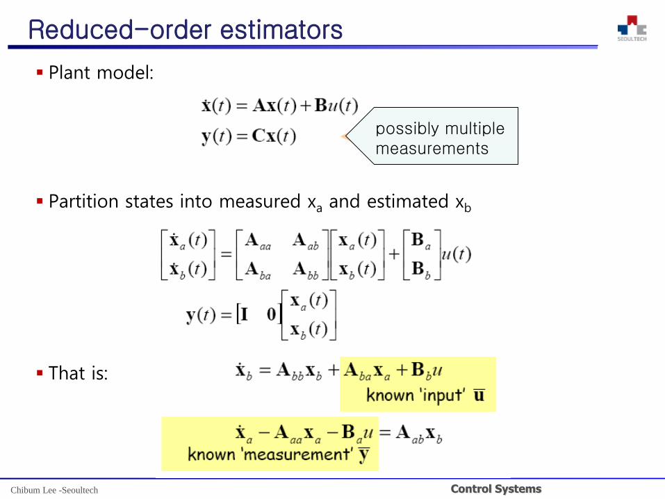
Reduced-order estimators
Plant model:
Partition states into measured xa and estimated xb
That is:
possibly multiplemeasurements

Control SystemsChibum Lee -Seoultech
Reduced-order estimators
Hence, observer:
Now, is in principle known, but
derivative term is a problem: difficult to realize
So, introduce a change in variable:

Control SystemsChibum Lee -Seoultech
Reduced-order estimators

Control SystemsChibum Lee -Seoultech
Error dynamics
Estimation error
That is,
Hence, design Lr as before, by selecting poles for Abb − LrAab
Design: Lr = place(A_bb’, A_ab’, dep)’

Control SystemsChibum Lee -Seoultech
Example 7.26

Control SystemsChibum Lee -Seoultech

Control SystemsChibum Lee -Seoultech

Control SystemsChibum Lee -Seoultech
Selection of estimator poles
CL char. poly:
The estimator poles (roots of aL(s) = 0) are usually chosen to be
between 2 to 6 times faster than the controller poles (roots of aK(s)
= 0)
Clearly there is no direct effect of choosing faster estimator poles
on control effort. However, consider the effect of sensor noise.
Assume that the sensed output is . The estimation
error dynamics then become:
Thus, the higher estimator gains required to produce faster
estimator dynamics will further amplify the sensor noise, thereby
corrupting the state estimates

Control SystemsChibum Lee -Seoultech
Symmetric root locus for SISO system estimator
Estimator dynamics with 'process noise' w and 'sensor noise' v :
The process noise w can represent unknown disturbances and errors
in the plant model parameters
Recall the estimator equations:
If w is large:
• our plant model is uncertain, and hence a poor predictor
• we would put greater emphasis on the sensor data to correct the model
predictions larger L, faster estimator poles
If v is large:
• our measurements are uncertain, and hence provide poor corrections
• we would put greater emphasis on the model predictions smaller L,
slower estimator poles

Control SystemsChibum Lee -Seoultech
Symmetric root locus for SISO system estimator
In optimal estimation theory
• the process noise is modeled as white noise with variance
• the sensor noise is modeled as white noise with variance
The estimator pole locations which will minimize the variance of the
state estimation error can be found from the solution of the
symmetric root locus (SRL) equation:
where is a measure of the plant model uncertainty
relative to the measurement uncertainty, and
is the plant transfer function from the process noise input to the
measured output
If the process noise w and control input u are additive (Bw = B), the
same SRL can be used for controller and estimator pole selection