U.S. Department of Transportation Federal Railroad Administration

Control of Rail Integrity By Self-Adaptive Scheduling of Rail Tests

Office of Research and Development Washington, DC 20590

O. Orringer U.S. Department of Transportation Research and Special Programs Administration Transportation Systems Center Cambridge, MA 02142

DOT/FRA/ORD-90/05 June 1990 Final Report

This document is available to the public through the National Technical Information Service, Springfield, Virginia 22161

This is a facsimile, reproduced from a scanned copy of the original report. Some differences between this facsimile and the original may be found. For example, known errors in the original

report have been corrected using word processing software.

NOTICE

This document is disseminated under the sponsorship of the Department of Transportation in the interest

of information exchange. The United States Government assumes no liability for its contents or use thereof.

NOTICE

The United States Government does not endorse products or manufacturers. Trade or manufacturers’ names appear herein solely

because they are considered essential to the object of this report.

Technical Report Documentation Page 1. Report No.

DOT/FRA/ORD-90/05

2. Government Accession No.

3. Recipient’s Catalog No.

5. Report Date

June 1990

4. Title and Subtitle

Control of Rail Integrity by Self-Adaptive Scheduling of Rail Tests 6. Performing Organization Code

DTS-76

7. Author(s)

O. Orringer

8. Performing Organization Report No.

DOT-TSC-FRA-90-2

10. Work Unit No. (TRAIS)

RR919/R9001

9. Performing Organization Name and Address U.S. Department of Transportation Research and Special Programs Administration Transportation Systems Center Cambridge, MA 02142-1093

11. Contract or Grant No.

13. Type of Report and Period Covered Final Report May 1989 – December 1989

12. Sponsoring Agency Name and Address U.S. Department of Transportation Federal Railroad Administration Office of Research and Development Washington, D.C. 20590

14. Sponsoring Agency Code

RRS-30

15. Supplementary Notes

16. Abstract

A guide for the scheduling of in-service tests of rail to detect defects is presented. The guide is designed for self-adaptation to changing track conditions, as reflected by the total rate of defect occurrence per test, the rate of “service” defect occurrences (i.e., defects found by means other than scheduled tests), and the tonnage of traffic carried between tests. The relation of numbers in the guide to the results of earlier studies is summarized. Conventions for using the guide are explained. Example applications based on both simulated and actual track conditions are presented. Several suggestions are offered for development of a performance specification based on the guide.

17. Key Words Crack Growth, Damage Tolerance, Fatigue, Rail, Railroad, Structural Integrity

18. Distribution Statement

DOCUMENT IS AVAILABLE TO THE PUBLIC THROUGH THE NATIONAL TECHNICAL INFORMATION SERVICE, SPRINGFIELD, VIRGINIA 22161

19. Security Classif. (of this report) Unclassified

20. Security Classif. (of this page) Unclassified

21. No. of pages

96

22. Price

Form DOT F 1700.7 (8-72) Reproduction of completed page authorized

PREFACE

This report brings together the results of ten years of research on the structural integrity of rail. The research is sponsored by the Office of Research and Development of the Federal Railroad Administration (FRA) as a part of the FRA Track Safety Research Program. The program objective is to develop technical information which can be used to support rational criteria for the preservation of safe operations on railroad tracks. The research is managed and in part performed by the DOT Transportation Systems Center (TSC) as the FRA/TSC Rail Integrity Project.

Many railroad industry organizations, independent research laboratories, and universities have contributed to the Rail Integrity Project. The American Railway Engineering Association (AREA) provides the experience of active railroad chief engineers to steer the project under the auspices of the FRA/AREA Ad Hoc Committee on Track Performance Standards. The Atchison, Topeka, and Santa Fe, Bessemer & Lake Erie, Boston & Maine, Burlington Northern, Chessie System, Kansas City Southern, Norfolk Southern, Southern Pacific, and Union Pacific railroads have donated test rails, provided revenue track test sites, and shared rail defect report records to support the project. The Association of American Railroads (AAR) has made major contributions through its management of rail integrity experiments at the Transportation Test Center and with laboratory tests and analytical work at the AAR Chicago Technical Center. The project has also benefited from exchanges of technical information with the office of Research and Experiments of the International Union of Railways.

The Battelle Columbus Laboratories have made numerous laboratory research contributions, most notably in the advancement of experimental techniques for measuring rail residual stress. Arthur D. Little, Inc., has developed preliminary fracture mechanics models of bolt hole crack and vertical split head defects. Other independent laboratories and academic institutions whose work has contributed directly or indirectly to the project include: the Analytic Sciences Corporation; Ensco, Inc.; Foster-Miller, Inc.; the IIT Research Institute; Lehigh University; Northwestern University; the Oregon Graduate Center; the Southwest Research Institute; Tufts University; the University of California at Los Angeles; and Vanderbilt University.

The Massachusetts Institute of Technology and the Instron Corporation have made key contributions toward the understanding of load - interaction effects on crack growth in the rail head and in fracture stability analysis of roller straightened rails. Under the auspices of the 1987 bilateral Science and Technology Exchange Agreement between the U.S. and Poland, the Central Research Institute of the Polish State Railways has recently started a series of controlled full-scale laboratory tests to investigate the relation between railmaking process parameters, wheel-rail contact loads, and rail residual stress; a parallel project at the Politechnika Krakowska has led to the development of a novel computational method for predicting these stresses.

iii

iv

TABLE OF CONTENTS

Section Page

1. INTRODUCTION ........................................................ 1

2. RAIL DEFECT FORMATION, GROWTH, AND DETECTION ........................ 3

................................................ 42.1 Defect Behavior

........................................ 52.1.1 Defect formation

.......................................... 212.1.2 Defect growth

.................................................. 312.2 Rail Testing

........................................ 332.2.1 Detection model

...................... 362.2.2 Correlation with field experience

................................. 402.3 Maintenance of Rail Integrity

3. TEST SCHEDULING GUIDE .............................................. 46

.......................................... 463.1 Adjustment Procedure

............................................. 473.2 Performance Chart

.......................................... 473.3 Example Applications

4. BEHAVIOR STUDIES .................................................... 55

............................................. 554.1 Simulation Studies

.............................................. 704.2 Railroad Studies

5. DISCUSSION .......................................................... 75

...................................... 755.1 Treatment of Double Track

.................................... 775.2 Definition of Line Segment

................................. 795.3 Treatment of Seasonal Effects

........................................... 815.4 Compliance Criteria

6. CONCLUSIONS ........................................................ 82

REFERENCES ........................................................... R-1

v

LIST OF ILLUSTRATIONS

Figure Page 1 Rail Defect Formation and Disposition................................ 3 2 Rotating Bending Fatigue Test........................................ 8 3 Fatigue Life Versus Alternating Stress Amplitude..................... 9 4 First Percentile S-N Curves for Rail Steel........................... 11 5 Modified Goodman Diagram for Rail Steel.............................. 13 6 Statistics of Sampling for Defect Rate............................... 18 7 Measured Clustering Tendencies on Ten Track Sites.................... 19 8 Actual Versus Theoretical Clustering Tendencies...................... 19 9 Effect of Crack Growth on Rail Integrity............................. 21 10 Potentials for Reduction of Detail Fracture Life..................... 25 11 Potentials for Variation of Detail Fracture Life..................... 26 12 "Winter Bolt Hole Crack" Mechanism................................... 28 13 Detection Performance Curve.......................................... 33 14 Masking Effect of Shell.............................................. 36 15 Detail Fracture Detection Performance Model.......................... 37 16 Ratio of Service to Detected Defects................................. 41 17 Idealized Scheduling Programs........................................ 42 18 Master Scheduling Curve.............................................. 43 19 Dependence of Service Defect Rate on Test Schedule................... 44 20 Variation of Detection Performance................................... 44 21 Effect of Behavior Deviations on Performance......................... 45 22 Rail Test Scheduling Performance Chart............................... 48 23 Hypothetical Application............................................. 50 24 Procedure for Off-Scale Adjustment................................... 5l 25 Example of Low Defect Rates.......................................... 52 26 Application Based on Annual Data..................................... 54 27 Simulation of Medium Density AMF Line ................................ 56 28 Simulation of a Heavy Haul Line...................................... 58 29 HDMF Baseline Simulation............................................. 62 30 One Fifth of Rails Subject to Fatigue................................ 63 31 Better Rail.......................................................... 64 32 Worse Rail........................................................... 65 33 Severe Maintenance Problem........................................... 66 34 Severe Cold Weather Effect........................................... 67 35 Better Test Equipment................................................ 68 36 Summary of Simulation Study Results.................................. 69 37 ATSF Study of Suggested Versus Actual Interval....................... 72 38 Suggested Interval Versus Annual Tonnage............................. 72 39 Actual Interval Versus Annual Tonnage................................ 73 40 Suggested Versus Actual Interval on High-Density Track............... 74 41 Track and Traffic Patterns........................................... 77 42 Distribution of Track Segment Lengths in the Study................... 78 43 Matching Test Cycles to Annual Records............................... 80

vi

LIST OF TABLES

Table Page

1 Rail Fatigue Defects ................................................ 6 2 Distribution of Common Fatigue Defects by Type ...................... 7 3 Typical Sources of Rail Defect Clusters ............................. 20 4 Predicted Versus Observed Detail Fracture Growth Life ............... 24 5 Factors Affecting Detail Fracture Growth ............................ 25 6 Comparison of Detail Fracture Detection Performance Model with CP Specification ............................. 38 7 Defect Size Ranges and Detection Probabilities ...................... 39 8 Summary of HDMF Simulations ......................................... 59 9 Scope of ATSF Study ................................................. 71 10 Scope of High-Density Track Studies ................................. 74

vii

GLOSSARY OF SYMBOLS A - Defect size D - Detected defect rate F - Cumulative probability function f - Probability density function N - Fatigue life P - Detection probability p - Detection probability function S - Stress; service defect rate SA - Alternating stress amplitude SM - Mean stress Smax - Maximum stress Smin - Minimum stress U - Ultimate tensile strength x - Longitudinal rail coordinate; expected number of defects y - Lateral rail coordinate z - Vertical rail coordinate α - Weibull probability model shape factor β - Weibull model characteristic life parameter λ - Average defect density

viii

EXECUTIVE SUMMARY

This report is the second in a series which brings together the results of ten years of rail integrity research. The term "rail integrity" refers to control of the risk of rail failures which can be caused by defects in the rail metal. Most such defects in modern U.S. track arise from metal fatigue, i.e., they are cracks formed and enlarged by the repeated passage of trains over the rail. The research objective is to provide the basis for rail integrity specifications. The first report, published in December 1988, summarized the results of tests and analyses which characterize the rate of growth of detail fractures under the range of service conditions found on U.S. railroad tracks. (Detail fractures are the most common fatigue defects found in modern track.)

This report combines the crack growth research with other results to provide the basis for a specification to control the scheduling of rail tests in service. Rail testing refers to the continuous search of rail to find defects, in order to allow time for remedial actions to be taken ahead of rail failure. (Remedial actions encompass protection or repair of discovered defects and removal of defective rails from track. A later report will present the basis for a specification on remedial actions.)

The current federal Track Safety Standards (49 CFR 213) set forth a minimum requirement for annual testing of all rail in Classes 4 through 6 track and in Class 3 track over which passenger trains operate. (These specifications are equivalent to requirements to test all rail on which freight trains operate at more than 40 mph or on which passenger trains operate at more than 30 mph.) The major U.S. railroads test heavily used track more often and conduct annual tests on more low-speed track than required by the standards.

The idea which motivates the rail integrity scheduling specification is that test requirements should be flexibly related to actual track usage. Overall rail safety can be improved by extending the coverage to all track carrying traffic faster than 25 mph, while allowing the frequency of testing to vary in proportion to track usage and rail condition.

The research results have provided quantitative knowledge of the three most important factors which relate test schedules to rail integrity: the rate at which rail fatigue defects can be expected to form; the rate at which these defects can be expected to enlarge; and the net (equipment and operator) efficiency of detection by testing conducted in accordance with current nondestructive inspection technology and practices.

These results have been integrated into a performance chart which can be used to guide the scheduling of rail tests. The data required to use the chart consists of information available from records already being kept by the railroads: the dates of recent tests and annual statistics of traffic tonnage, detected defects, and defects discovered

ix

by other means ("service" defects). The chart is based on a performance target of one service defect between tests per ten track miles, a number which reflects the current national average.

The behavior of the performance chart has been studied by means of simulations and practical evaluations. The simulations were conducted by means of mathematical models representing averages and deviations of the three main factors (defect formation, growth, and detection efficiency). The practical evaluations consisted of trial "paper" applications of the chart by participating railroads, using actual records and comparing the test frequencies suggested by the chart with present practice. The simulation studies showed that the chart is a flexible guideline which adjusts the test frequency to adapt to long-term changes in service conditions. The practical evaluations suggest that room does exist to rebalance present practices toward more frequent testing of heavily used track and less frequent testing of lightly used track.

The performance chart has thus been established as an element suitable for use in a rail integrity specification. However, two additional elements are required to form a complete specification: procedural rules and terms of application. Procedural rules are required to deal with certain exceptions to the basic graphical construction steps associated with the chart. These rules were formulated during the study but still require precise language for clarification. Terms of application are required to deal with certain other practical issues. These issues are: how to account for annual records on lines consisting of double or alternating double and single track; how many miles of track should be considered as an entity ("line segment") for the purpose of applying the specification; and how to match annual records with test schedules that do not coincide with calendar years. Preliminary terms of application have been formulated but require some further study and precise language before they can be accepted as practical elements of a rail integrity specification.

A good specification should also meet one more condition: avoidance of unnecessary paperwork. The rail integrity specification outlined in this report can be implemented without requiring any railroad reports or record keeping beyond the records already being kept. Also, the railroads need not be required to keep any records of calculations made to apply the specification. FRA track inspectors would have to do some calculation paperwork to determine that a railroad's test schedules are in compliance with the specification, and railroads might want to work through the specification procedures at their own option in order to assess the effect of the minimum requirements on their test schedules. In both cases, however, the work can likely be limited to isolated line segments where track engineers and inspectors judge a potential for exceptions to exist.

x

1. INTRODUCTION

This report describes a self-adaptive guide for scheduling rail tests on U.S. railroads. The guide was developed under the rail integrity project, a part of the ongoing track safety research program sponsored by the Office of Research and Development of the Federal Railroad Administration.

The guide is based on current knowledge of rail defect behavior and the performance of equipment used to detect rail defects. Section 2 summarizes the knowledge and how it has been used to derive working rules for the scheduling guide.

The guide is presented in the form of a performance chart which a track engineer can use to help set the interval from the test just conducted to the next test. To apply the guide to a specified stretch of track, the engineer must know the interval (in gross tons of traffic) between the test just conducted and the preceding test. He must also know the number of service defects and breaks found in that interval, the number of defects found in the test just conducted, and the mileage of track involved. These items of information are normally contained in the records kept by railroad track departments.

Section 3 describes the guide. The relations between the input data, defect behavior characteristics, and the working rules are explained. The guide chart format is explained, and some example applications are presented to illustrate how the chart is used.

The guide is intended to function like a self-adaptive control system. Like all control systems, it embodies a performance goal and triggers a response if the goal is not met. In the present case, the goal is a maximum number of service defects and breaks per track mile between tests. If the maximum is exceeded, the response is to decrease the test interval. Conversely, a longer interval between tests is allowed if the actual rate is much lower than the goal.

The working rules which govern the response are based on certain assumptions about the average behavior of rail defects and the equipment used to detect them. However, supporting studies have shown that rail defect behavior can vary widely about the average, and that equipment behavior is also variable and difficult to accurately quantify. Therefore, the guide has been designed so that the response rules are, in effect, automatically changed to cope with deviations of the actual behaviors from the assumed averages. This characteristic is the self-adaptation property.

How well do the working rules function? This question can only be answered by studying the way the guide behaves. Section 4 presents the results of two such studies. In the first, mathematical models were used to simulate rail defect and detection equipment behavior on a hypothetical stretch of track, and the reactions of the guide were

1

studied under simulated deviations from the underlying assumptions. In the second study, the guide was retrospectively applied to actual railroad lines, and its prescriptions for the next test interval were compared with the railroads' actual practices.

It is hoped that the guide described here, or some similar version, may eventually provide a useful basis for a flexible specification for scheduling rail tests. Such a specification could improve safety and reduce test costs by allowing a redistribution of rail testing to concentrate on track with relatively high rates of defect occurrence.

However, it should be recognized that the guide alone does not constitute a specification. Since the working rules are relatively simple, the guide is unlikely to provide a practical response to every situation. Therefore, some room must be left for the track engineer to exercise his judgement in setting the rail test schedule, using the guide as a supporting tool. Also, the guide contains no information about how to group track for its application, and there remain some practical questions about its implementation. Section 5 discusses these topics. Section 6 summarizes some conclusions and recommendations.

2

2. RAIL DEFECT FORMATION, GROWTH, AND DETECTION

The rail defect population in a stretch of track fluctuates as service time passes. Railmaking errors, handling or service damage, and the cumulative effects of metal fatigue add defects to the population. Repeated wheel loads are the source of the metal fatigue and also cause many kinds of defects to grow in size after they have formed. Rail tests, visual inspections, and signal circuit interruptions detect defects, which are then removed from service when the affected rails are repaired or taken out of track. Undetected defects may also be removed from service during scheduled rail renewals, e.g., for replacement of worn rails.

Figure 1 illustrates the general sequence of defect formation and disposition. The widths of the various paths in the diagram are proportioned to the relative numbers of defects in a population one would expect in rail well into its normal service life. Thus, metal fatigue is indicated as the greatest source of new defects, and previously formed defects are represented as ranging from small to large size with some having grown sufficiently large to become service breaks.

FIGURE 1. RAIL DEFECT FORMATION AND DISPOSITION

3

The possible outcomes are indicated along the bottom of the diagram. Undetected defects of all sizes may be removed as a consequence of rail renewals. Rail tests may detect defects of all sizes, while visual inspections generally detect only large defects or service breaks, and signal interruptions detect only service breaks. These detections are the only indicators of the existing defect population, and interpretation is complicated by the time delay between formation and detection.

An ideal system of inspections would detect only those defects which would pose risks of derailment if not removed before the next inspection. The ideal cannot be attained in practice, but real inspection strategies can be devised to keep derailment rates low. Such strategies can be developed from an understanding of how rail defects and inspection methods behave with respect to each other. Sections 2.1 and 2.2 consider these topics separately. In Section 2.3, the two aspects are brought together to formulate the basic concepts of maintaining the integrity of rail in the presence of growing defects.

2.1 Defect Behavior

Formation and growth are the two key aspects of rail defect behavior. Formation determines the numbers of defects which can be expected to enter the population, the intervals of service life over which they appear, and the distribution of their locations in track. Growth determines the intervals of service life over which defects can be expected to evolve to larger sizes if not detected. Tonnage, usually expressed in millions of gross tons (MGT), provides the most consistent measure of the effects of service on both formation and growth. Rail service ages are commonly expressed in accumulated MGT and traffic densities in annual MGT (i.e., MGT per year). There are seasonal effects on defect behavior, however, which must be accounted for in terms of calendar time.

Defect behavior has been studied by collecting data from the field and by constructing physical/mathematical models. Field data is used to establish the general ranges of defect behavior and to provide a check on the realism of models. The models are used to isolate the effects of individual service variables and to extrapolate the behavior ranges to combinations of variables for which field data is not available.

The framework for a model of a rail defect is generally adapted from a similar model of a phenomenon observed in the laboratory. For example, models of MGT required to form a defect may be adapted from models of rotating-bending fatigue tests performed on round-stock specimens; models of MGT required to grow a defect are generally adapted from models of through-crack propagation tests performed on flat-stock specimens. Laboratory test conditions are directly specified in terms of numbers of alternating stress cycles and the level of mean stress applied to the specimen. Therefore, adaptation of laboratory models to rail defects requires some additional calculations to relate gross tonnage to wheel-rail loads and loads to stresses in the rail. The resulting collections

4

of alternating stress cycles and mean stress levels are referred to as stress spectra. Like the models of defect behavior, calculations which produce estimates of stress spectra must be checked against field data on service loads.

2.1.1 Defect formation

The earliest occurring defects generally come from railmaking errors. Piped rails, base seam defects, and transverse fissures are well known examples. Modern railmaking practices such as ingot hot-topping, continuous casting, and careful control of the rail temperature during rolling have greatly reduced the incidence of piped rail and base seam defects. Reduction of retained hydrogen by means of controlled cooling or vacuum treatment has virtually eliminated transverse fissures.

These kinds of mill defects are still found occasionally, but they tend to occur in relatively low numbers and at random, as results of occasional lapses from established railmaking practice. Piped rail and base seam defects generally appear in the first few MGT of service, while the formation of transverse fissures may be spread over much of the rail service life by variations in the density of hydrogen flakes which precipitate in the rail head.

Handling or service damage creates defects at random, as either isolated or group occurrences. Broken base defects, which generally come from accidental maul strikes on the flange, are examples of isolated handling-damage defects. Crushed heads, which may be caused by extreme overloads from defective wheels, are examples of defects induced by service damage and occurring in groups. Engine burns are examples of service-induced damage which may occur in groups or isolated pairs. While engine burns per se should not be considered as defects for safety purposes, a small proportion of them may develop into engine burn fracture defects which can grow as transverse cracks in the rail head.

Among all the kinds of rail defects caused by processes other than metal fatigue, defective welds in continuous welded rail (CWR) are the most prevalent. Most of these defects occur in the thermite field welds used to join CWR strings in track. Some weld defects consist of only a few small round void bubbles and are innocuous. Others form as medium-sized flat-shaped voids or as lack-of-fusion defects. Isolated occurrences of medium voids may result from sand pockets formed by accidental entrainment of mold material in the molten thermite charge. Lack-of-fusion defects between the weld material and the rail ends may occur in groups because of inadequate attention to welding practices (insufficient preheat, improper rail-end gap, etc.). Sand-pocket and lack-of-fusion defects can quickly evolve into sharp cracks, which tend to grow in the transverse section of the rail in service.

5

Several kinds of rail defects are products of metal fatigue, either from direct effects of rolling-load contact stresses in the rail head or from the effects of loads at rail ends. Table 1 categorizes these defects by source and relative numbers. In general, they tend to form in greater numbers as rail service age increases, but their rates of occurrence often fluctuate. They may be randomly distributed along the track, or they may concentrate in clusters for a variety of reasons. The fatigue defects also exhibit a consistent tendency to grow in service.

Defect chronology in track is a blend of the various kinds of events outlined above. Consider track in which the rail has just been totally renewed, at which point the service age clock has been reset to zero. Mill and/or weld defects first appear somewhat later, but are found in declining numbers as the rail ages. After these defects have been exhausted, there may occur a defect-free period of service, until the first fatigue defects appear. As the rail continues to age, fatigue defects form in rising numbers, and transient episodes of defects caused by handling and/or service damage may also occur. Maintenance may also include partial rail renewals (e.g., on curves), and what was originally a uniform stretch of rail becomes a set of groups with different ages. The defect occurrence rate for the whole stretch of track will then continue to fluctuate in response to the natural variations of fatigue defect formation, the random introduction of other kinds of defects, and the rise, decline, and disappearance of rail groups as fatigue defect sources.

TABLE 1. RAIL FATIGUE DEFECTS

6

Two studies of rail defect reports have been made to identify occurrence patterns. The first study encompassed roughly 25,000 defects on 8,200 track miles in segments selected by four participating railroads (Orringer and Bush 1983; Mack et al. 1984). The criterion for selecting a segment was a higher than desirable rate of defect occurrence, as defined by the judgement of each railroad. Four to six years of service on each railroad in the period 1974 to 1981 were covered, and the reports were aggregated by calendar year. For each year, the defects were classified by type and track location (milepost). In the second study, a smaller sample of early 1980s defect reports from selected main and siding track of two railroads was classified by defect type (Association of American Railroads, Engineering Economics Division, unpublished data, 1985). These results were later compared with those of the earlier study (Orringer 1988).

Although significant differences between different track segments were found, both studies confirmed the qualitative chronology described above. In general, from 70 to 95 percent of the defects reported on any of the track segments were found to belong to the fatigue defect group, and more than 90 percent of the fatigue defects were the types listed in Table 1 as "common". A major difference between bolted-joint rail and CWR was also noted, viz: the distribution of defects by type (Table 2).

TABLE 2. DISTRIBUTION OF COMMON FATIGUE DEFECTS BY TYPE

The statistics on defect types suggest that models of fatigue crack formation are appropriate tools for correlating observations of rail defect occurrence rates. Such models begin with the correlation of laboratory experiments, e.g., on the measurement of the number of alternating stress cycles required to form cracks in rotating bending specimens tested at different stress amplitudes. The specimen is subjected to four-point bending by loads applied through the bearings in which it rotates; the applied stress is greatest at the specimen surface and is a pure alternating compress ion-tens ion cycle of constant stress amplitude (Figure 2). Cracks form at the surface, and the fatigue life is usually defined as the number of cycles required to break the specimen.

7

FIGURE 2. ROTATING BENDING FATIGUE TEST

The rotating-bending fatigue test was actually devised to investigate a problem of axle fatigue cracking which occurred early in the history of railroad engineering (Wohler 1858, 1860, 1866, 1870). It is apparent from the figure that the arrangement for the rotating bending test was taken directly from the service loading applied to a railroad car axle.

Other types of laboratory fatigue tests have since been devised to simulate different kinds of service conditions. In particular, the development of servo-controlled mechanical testing equipment and self -aligning grips has led to the widespread use of flat-stock specimens in push-pull tests, where the conditions can be set for pure alternating stress or for a combination of alternating stress with a tensile or compressive mean stress.

The Association of American Railroads (AAR) and the Federal Railroad Administration (FRA) have sponsored a number of research studies on the fatigue properties of rail steel, and the results have been summarized in several publications (Stone and Knupp 1978; Steele and Reiff 1982;

8

Orringer and Bush 1983; Orringer, Morris, and Steele 1984). Two major characteristics of rail steel fatigue life under pure alternating constant-amplitude stress are found: (1) the fatigue life generally increases as the alternating stress amplitude SA decreases; and (2) at any particular value Of SA the lives of individual specimens may vary by a factor of two to as much as ten. Such results are typical for most metal alloy products and reflect the dependence of fatigue life on aggregations of random events at the atomic level in the metal crystal structure.

A schematic illustration of the fatigue life trend for rail steel subject to pure alternating stress is shown in Figure 3. Also indicated are some of the ways in which models are used to correlate a typical set of life data, which covers only a few discrete values of stress amplitude. The average (or 50th percentile) life for each tested stress amplitude is calculated from the data, and these averages can generally be fitted with a straight line when the fatigue life axis is logarithmically scaled. The linear relation is generally found to correlate the life performance for stress amplitudes between about 25 to 80 percent of the metal's ultimate strength (a range of 30 to 90 ksi for rail steel of standard composition). At the lower limit, the scatter in the life data is the greatest, and many of the specimens do not break within the maximum testing time allowed (usually five to ten million cycles). Arrow symbols indicate these results as "runouts", and the bilinear fit shown in the figure is referred to as the "S-N curve" for the material.

FIGURE 3. FATIGUE LIFE VERSUS ALTERNATING STRESS AMPLITUDE

9

The average S-N curve is useful for comparing test results from different laboratories but does not represent typical service usage of rails, for which wear generally limits the useful life to between 500 and 1,000 MGT. These apparently long lifetimes are, however, short in comparison with the amount of service which would be equivalent to the average fatigue life of rail steel. Therefore, the first percentile S-N curve is often used to model rail fatigue life. First percentile life means the time at which one percent of a large sample of specimens can be expected to have formed a crack.

As indicated in Figure 3, the first percentile S-N curve generally lies to the left of the laboratory test data and must be estimated by means of statistical analysis. The AAR uses an extreme-value type of probability model (Weibull 1951) for this purpose. The formation of a fatigue crack is an extreme-value process, in the sense that each life measurement reflects the performance of the weakest part of one test specimen (Weibull 1961). The Weibull model expresses the cumulative probability F(N) for the fatigue life N as follows:

(1) ( / )( ) 1 NF N eαβ−= −

where the shape factor α and characteristic life β are the model parameters. These parameters resemble the Gaussian standard deviation and average, respectively, and are estimated from a set of life data by means of standard statistical formulae or graphical methods (Hahn and Shapiro 1967; Breiman 1973). In the schematic illustration in Figure 3, for example, a set of Weibull model parameters would be found for each of the four sets of life data, and eq. (1) would then be used to calculate the first percentile life for each of the four tested stress amplitudes. A straight line fitted to these values would provide the sloping part of the first percentile S-N curve. Figure 4 illustrates the first percentile S-N curves for rail steel obtained from the results of three independent investigations (Jensen 1950; Fowler 1976; Rice and Broek 1982).

The Weibull model has also been used to correlate rail defect data in a study of six locations on two railroads (Besuner et al. 1978). Each site was selected to have as nearly uniform rail as possible, and defect occurrences were collected up to the second percentile (i.e., two percent of the total number of rails at each site having developed defects). The six sites were fitted with individual Weibull models, which were found to have shape factors α ranging from 2.9 to 5.5, with α = 3.6 providing the best overall fit. When the 3.6 shape factor was assumed for all the sites, the characteristic lives β were found to range from 1,200 to 3,000 MGT. The loads and rail stresses at these sites were not of constant amplitude but did lie within the general category of “70-ton" (i.e., mixed general freight) traffic. A later study compared the results

10

FIGURE 4. FIRST PERCENTILE S-N CURVES FOR RAIL STEEL

from these and similar locations with results from the FAST track1 (Steele and Reiff 1982) to show the reduction of rail fatigue life caused by the heavier (100-ton) FAST traffic.2 These results were found to be well fitted by a shape factor α = 3 and characteristic lives β = 2,000 MGT for 70-ton traffic and β = 1,000 MGT for 100-ton traffic.

How well does the Weibull model represent the rate at which rail fatigue defects form in typical service environments? The model parameters have been derived from field data that covers a variety of defect types, including some mill and damage defects. The range of shape factors for individual track sites suggests fatigue lives that are strongly affected by subtle differences in rail quality and/or service conditions. The aggregate of the field data samples is extremely small: of the order of 0.01 to 0.1 percent of the national rail network.

1 Facility for Accelerated Service Testing, a 4.7-mile dedicated loop at the U.S. Transportation Test Center, Pueblo, Colorado.

2 The 70- and 100-ton figures refer to nominal useful carload capacities. The corresponding axle loads at maximum rail weight are 25 and 33 tons, respectively.

11

Under these circumstances, it is necessary to have some independent verification that the proposed formation model (α = 3; β = 2,000 MGT for mixed freight or 1,000 MGT for FAST traffic) bears a reasonable relation to average conditions. One way to provide such confidence is to compare the first percentile fatigue life predictions of the formation model with those obtained by combining the first percentile laboratory S-N curve with stress spectra constructed from rail mechanics. In order to make service life predictions from laboratory S-N curves, however, the effects of different values of mean and alternating stress must be rationally combined, and triaxial stress states3 must be taken into account.

The effect of mean stress on constant-amplitude fatigue life has been studied in the laboratory and can be summarized on the so-called modified Goodman diagram, in which constant-life lines are cross-plotted with respect to nondimensional axes SA/U and SM/U, where SA, SM, and U are respectively the alternating stress amplitude, the mean stress, and the material ultimate strength.

Figure 5 illustrates a modified Goodman diagram constructed from the Jensen S-N curve shown in Figure 4. The Goodman life lines are extrapolated into the left half of the diagram, where the mean stress is compressive, because most of the laboratory experiments are performed under mean tension. It is customary to make level extrapolations, i.e., to assume that a compressive mean stress has no benefit. However, some rolling contact experiments on ball bearings have shown that mean compression tends to increase fatigue life, suggesting the linear extrapolation indicated by the dashed lines (Sines and Waisman 1959). The line extending left and upward from the origin indicates the combinations of mean and alternating stress in the rail head due to the effect of rail bending. The position of this line illustrates the point that predictions of rail head defect fatigue life based on laboratory data must rely on extrapolation.

The effects of different values of mean and alternating stress applied to one specimen are combined by means of the so-called Palmgren-Miner damage summation rule (Palmgren 1924; Miner 1945). Let N be the fatigue life corresponding to one pair of values (SA, SM), and suppose that some smaller number of cycles, n, is actually applied. Then the quantity n/N is defined as the fraction of life consumed by the application; this definition is consistent with the results of experiments at constant mean and alternating stress but adds no new

3 A triaxial state refers to the simultaneous presence of stresses acting in different directions. For example, live-load stresses in the rail head directly under the center of wheel contact include lateral and vertical as well as longitudinal components.

12

FIGURE 5. MODIFIED GOODMAN DIAGRAM FOR RAIL STEEL

information. The Palmgren-Miner rule is based on three hypotheses about situations in which different stress combinations (SA1, SM1), (SA2, SM2), etc., are applied to one specimen:

(1) The fraction of life consumed by each cycle does not depend on the preceding cycle history.

(2) The fraction of life consumed by the ith stress combination is proportional to the number of cycles applied in that combination, ni/Ni.

(3) A fatigue crack forms when the sum of life fractions consumed by all stress combinations, nl/Nl + n2/N2 + ..., is equal to one.

The Palmgren-Miner rule has no physical or mathematical basis and, in fact, does not work well when the history of applied stress has a pronounced trend. For example, laboratory experiments have shown that the actual fatigue life is shorter than predicted by the rule when the stress amplitudes steadily decrease and longer when they steadily increase.

The Palmgren-Miner rule is nevertheless a useful approximation when the history of applied stress has no pronounced trend, as is the case for rails subjected to repeated loads from similar trains. However, the results of laboratory experiments on rail steel specimens subjected to simulated service stress spectra (Rice and Broek 1982) suggest that the larger stresses tend to cancel the runout effect observed at smaller

13

stresses in constant-amplitude tests (see Figure 3). Therefore, the sloping segment of the S-N curve is generally extrapolated when rail fatigue life predictions are made.

The live-load stress spectra used to predict rail fatigue life are reconstructed from the mechanical model of a rail as a continuous beam on a continuous elastic foundation (Talbot et al. 1930; Timoshenko and Langer 1932; Hetenyi 1983). Minimum and maximum stresses are derived from the effects of rail bending under an isolated wheel load and at the first reverse bending point, respectively. The corresponding fatigue stress cycle is defined by:

max min

2AS SS −= max min

2MS SS += (2)

Field measurements of dynamic wheel load occurrences (Ahlbeck et al. 1980) provide the relative numbers of load levels (i.e., numbers of stress combinations) per MGT. The Palmgren-Miner life estimate in MGT is then given by 1/( Σ ni/Ni).

The first efforts to develop a fatigue life model based on rail mechanics made use of a published S-N curve and concentrated upon the effect of the alternating longitudinal stress amplitude associated with rail bending (Abbott and Zarembski 1978; Zarembski 1979). Bending stress was viewed as the logical choice for the model, since the tensile part of the stress cycle would tend to open a detail fracture. The fatigue life, calculated as a function of depth in the rail head, was found to increase as the bending stress amplitude decreased with depth below the crown. The calculated life at subsurface shell formation depths (typically 1/4 to 3/8 inch) appeared to be in reasonable agreement with service experience.

The ambiguity led to a search for a modified model which could predict the crack formation depth as well as the fatigue life. The effects of rolling contact stress, mean stress, and rail wear were added for this purpose, and the sensitivity of calculated life to various model assumptions was studied (Perlman et al. 1982).

The contact stress was based on the three-dimensional theory of elastic contact between two cylinders crossing at right angles (Hertz 1895), using wheel tape line and rail crown radii as is the practice for sizing wheels in relation to axle load. The contact stress calculations were confined to points in the rail head directly underneath the center of wheel contact: a locus along which the longitudinal, lateral, and vertical stresses Sx, Sy, and Sz are principal stresses.

The mean stress was modelled by an empirical summary of the residual stresses measured in samples of used rail taken from tangent track (Groom 1983). Residual stress builds up in the rail head as a result of plastic deformation in the contact zone near the running surface. Once established, however, the residual stress undergoes little or no change.

14

The effect of rail wear was modelled by shifting the contact and residual stress fields downward with respect to the unworn rail crown height. This feature of the model was intended to simulate the gradual exposure of subsurface material to the stress levels occurring nearer to the running surf ace, as would happen in the rail head. The stress fields were shifted at rates comparable to measured head height loss rates (typically 0.03 inch per 100 MGT).

Like the original model, the modified model took only longitudinal stresses into account. The curve of fatigue life versus depth did exhibit a definite minimum, which could be interpreted as a predicted crack formation depth, but the results were somewhat shallow (1/8 to 1/6 inch). The calculated life was again in rough agreement with service experience, but reexamination of the input data now revealed that a calculation based on average laboratory properties had been compared with first percentile service experience. In other words, a proper comparison would have led to a calculated life much shorter than the first percentile fatigue life inferred from the rail defect report data.

Reexamination of the study results also revealed two deficiencies in the mechanical fatigue model. First, contrary to expectations based on order-of -magnitude estimates, it appeared that the assumed wear rate had a strong influence, while residual stress had almost no effect on the fatigue life. Second, some obvious anomalies were found in the comparison of life calculations for different rail sections, e.g., the fatigue life of a 70 ASCE section apparently exceeded the lives of 115 RE and 132 RE sections. (These spurious results were found to be artifacts of using the section design crown radii as inputs.) At this stage of the development, it was also recognized that the fatigue life prediction ought to be based on shell formation, rather than upon the formation of detail fractures which actually branch from established shells. Accordingly, since shells tend to form in a nearly horizontal plane, the model should have been based on either vertical or triaxial rather than longitudinal stresses.

Further revisions of the model were the subject of a later study (Jeong et al. 1987). A typical value was arbitrarily adopted to represent the rail crown radius in place of the individual design values for different sections. Alternative revisions incorporating vertical and triaxial stresses were included in the study. In the triaxial version, effective mean and alternating stresses were calculated from the hydrostatic and octahedral stresses, respectively, in accordance with Sines,' hypothesis (Sines and Waisman 1959). In his original work, Sines had assumed an unlimited benefit effect of mean compressive stress, i.e., the constant-life lines were to be linearly extrapolated into the entire mean compression region of the modified Goodman diagram (Figure 5). Since no rail steel data could be found to justify an unlimited extrapolation, the extent of the assumed benefit was varied in the present study.

15

In the results initially obtained from the triaxial model, the effect of contact stress on fatigue life was so strong that none of the other variables appeared to have any influence. This result was especially troubling because the fatigue life was sensitive to an arbitrarily assumed input (rail crown radius). Therefore, the contact stress was revised by basing its calculation upon the Hertz theory of two-dimensional contact between a cylinder (representing the wheel) and a flat surface.

Comparison of the alternative models showed that the triaxial version gave better results than either the vertical or longitudinal uniaxial versions. When the first percentile Jensen S-N curve (Figure 4) was used, the triaxial model predicted crack formation at a depth of 1/6 inch and a fatigue life which varied from 70 to 200 MGT as the assumed extent of the mean compression benefit was varied from none to a limit at SM/U = -0.15, with live-load stresses representing mixed freight traffic.

The 70 to 200 MGT range of life predicted by the mechanics model can be compared with the first percentile life of 432 MGT from the Weibull model for mixed freight traffic (see eq. (1) with α = 3, β = 2,000 MGT). The shorter life from the mechanics model is consistent with its relation to shell formation. The Weibull model is based on data which include the tonnages required to grow defects to detectable sizes as well as to form them, and should thus be expected to exhibit a longer life. The reasonable agreement between fatigue life predicted by a mechanics model based on average inputs and fatigue life predicted by a Weibull model fitted to a small sample of field data suggests that the Weibull model does indeed represent average service conditions. A similar Weibull model (α = 3.1, β = 2,150 MGT) has been adopted by the AAR for use in the Rail Performance Model maintenance planning tool (Davis 1987).

Where are defects found in track? If one assumes that a defect is equally likely to occur at any location, then one would expect a statistically uniform density of defects per track mile, given a suitable definition of the length of track required to measure the density. The statistical description which fits the assumed situation is the Poisson probability distribution:

( )!

x

f x ex

λλ −= (3)

where λ is the average density and f(x) is the probability of finding x defects in a stretch of track of the chosen length. The Poisson distribution is a well established model for describing events which are equally likely to occur in any interval (Hahn and Shapiro 1967).

The following examples will illustrate the application of the Poisson model to the distribution of rail defects. Consider 100 miles of

16

track with an average density of 0.5 defect per mile. The Poisson model predicts4 that one should expect to find 61 miles with no defects, 30 miles with one defect, 8 miles with two defects, and one mile with three or more defects. In other words, one would expect to find all of the defects in only 39 percent of the track miles. However, the same track could just as easily be described as having an average density of 0.25 defect per half mile or one defect per two miles. The corresponding Poisson expectations would then be that 22 percent of the half miles, or 63 percent of the two-mile stretches should contain all of the defects.

The foregoing examples illustrate an illusion of clustering5 when sparse data is analyzed, especially the cases in which the average density is less than one event per unit of measure. Another way to look at the illusion is to consider what might happen if the defect count from a sample of (say) 20 track miles were used to infer the defect rate on the entire 100 miles. If the Poisson description is approximated, for the sake of simplicity, as 50 miles each containing exactly one defect instead of 39 miles with one or more defects, then the probability of encountering x defects in the 20-mile sample is given by the binomial distribution:

( )2020!( ) 0.5 1 0.5!(20 )!

xxf xx x

−= −−

(4)

As illustrated in Figure 6, eq. (4) shows that such a sample would be expected to give an apparent defect rate within ±10 percent of the true average half the time; another 48 percent of the time, the apparent defect rate may be as little as half or as much as twice the true average. Similar exercises with sampling lengths shorter than 20 miles would exhibit greater scatter in the apparent defect rate. Thus, although rates based on short samples might be useful for identification of local problems, they should not be compared with long-sample averages to establish general track conditions.

The Sperry Rail Service collects historical data on the density of defects detected by rail tests. A recent analysis of that data shows densities between 0.4 and 0.8 per mile based on annual miles tested, the higher and lower numbers reflecting the early 1970s and the mid 1980s, respectively (Thomas 1985).6 Since these numbers represent a national average, they suggest that one should expect evaluations of actual rail defect distributions to display the clustering illusion and sampling error characteristics described above.

4 The numbers have been rounded to the nearest whole mile in these examples.

5 There is also a real clustering effect which is discussed later.

6 The long-term fluctuation in the historical average has been discussed elsewhere (Orringer 1988).

17

–

FIGURE 6. STATISTICS OF SAMPLING FOR DEFECT RATES

PROBABILITY OF FINDING A GIVEN NUMBER OF RAIL DEFECTS IN A 20 MILE SAMPLE OF 100 TRACK MILES

NUMBER OF DEFECTS

AVERAGE DEFECT RATE = 0.5/MILE (10 DEECTS IN 20 MILES)

Some of the actual distributions have also been found to possess a true clustering property, a feature which the Poisson model does not account for. The differences between true and illusory clustering were brought to light by comparing measured occurrences of defects per mile with the Poisson expectation (Orringer and Bush 1983; Mack et al. 1984). Cases both more and less clustered than the Poisson model were found. Figure 7 illustrates the findings for ten stretches of track examined in one analysis (Orringer and Bush 1983). The upper chart plots the percentage of miles which contained at least 90 percent of the defects (the actual percentages are given for each case), and the lower chart shows the total length of each stretch. Figure 8 compares measured clustering tendency with the extent of clustering predicted by applying the Poisson model to the average defect density for each track site or group of sites per participating railroad (A through D in Figure 7). From these results it appears that factors other than random chance have an important influence on the location of rail defects.

18

FIGURE 7. MEASURED CLUSTERING TENDENCIES ON TEN TRACK SITES

FIGURE 8. COMPARISON OF ACTUAL AND THEORETICAL CLUSTERINGTENDENCIES

The occurrence pattern study revealed important differences between the illusory and real clustering characteristics. In the Poisson model, even though a small percentage of the track miles might contain all of the defects, those miles would be scattered at random throughout the whole stretch of track. Also, if repeated trials of the model were used to represent succeeding years, each of which had about the same average

19

defect density, there would be no correlation of which miles contained defects from one year to the next. Conversely, the defect occurrence pattern study showed that track miles containing defects had a strong tendency to remain organized in one or more groups, the locations of which persisted over the several-year span encompassed by the study.

In contrast to the Poisson model, the observed patterns suggested that it would be worthwhile to consider rail test allocation strategies that focus resources on cluster locations. Many railroads already have such strategies based on annual tonnage and rail age. Defect clusters were thus expected and were found in the defect occurrence study.

The study also revealed some unexpected sources of clusters associated with track construction and/or operational characteristics. Table 3 summarizes several examples, and railroad engineers can undoubtedly find others in their own track. The formulation of a universal model of clustering is impractical, but some useful general conclusions can be drawn about rail defect locations in track: (1) the existence of persistent clusters is probable and can be established by plotting defect reports by milepost; (2) examination of cluster locations may suggest refinement of rail test allocation and/or supplemental inspection; and (3) clusters with unusually high local densities may suggest maintenance and/or operating changes to reduce the defect formation rate.

TABLE 3. TYPICAL SOURCES OF RAIL DEFECT CLUSTERS

20

2.1.2 Defect growth

The fatigue defects (Table 1) and some of the other types grow in response to repeated wheel loads. The rate of growth depends on the defect type and the applied stresses, and in general, the rate increases as the defect grows. A defective rail is weaker than a normal rail, and in general, rail strength decreases as the defect grows. As the growth continues, the applied stresses will eventually exceed the rail strength and cause a failure. The defect is said to have reached its critical size at the point of failure.

Figure 9 depicts the preceding sketch of defect growth behavior. Also shown in the figure is a so-called "detectable size", i.e., a size for which there is some expectation that a rail test would find the defect. Implicit in the definition of detectable size is the idea that a rail test is unlikely to find smaller defects. It then follows that the tonnage required to grow the defect from detectable to critical size defines the window of opportunity to find the defect. This window is called the safe crack growth life.

FIGURE 9. EFFECT OF CRACK GROWTH ON RAIL INTEGRITY

Studies of defect growth behavior have concentrated on the detail fracture because it is the most common type of fatigue defect encountered in CWR. Early attempts to model the detail fracture were based on the linear elastic fracture mechanics (LEFM) model of an idealized circular or elliptical penny crack in an unbounded body subjected to longitudinal rail stress spectra estimated from the single cycle per wheel approach mentioned earlier, plus a mean tensile stress term to represent residual stress (Stone and Knupp 1978). One of these studies suggested that a doubling of the mean tensile stress could change the crack growth rate by three orders of magnitude. At a mean stress of 10 ksi the calculated crack growth life would exceed the rail wear life, but at 20 ksi the crack growth life would be reduced to a few MGT. This result heavily influenced the direction of later research, since tensile longitudinal residual stresses in rail heads appeared at the time to lie within the study bounds.

21

However, it was not clear how well a LEFM model of a f lat-surf aced constant-shape crack represented detail fracture behavior, since detail fractures are neither flat nor of constant shape. A sharp discontinuity is found at the origin where the detail fracture branches away from the overlying shell. The detail fracture surface is usually curved and only approximately aligned with the transverse section of the rail. Defects smaller than 10 percent of the rail head area (%HA) are in general half-ellipses extending downward from the overlying shell; defects from 10 to 50 %HA have the shape of a full ellipse; and defects larger than 50 %HA change to an irregular shape, with breakouts on the gage face and running surface, and with part of the defect extending into the rail web.

These obvious differences made it necessary to conduct experiments, as well as analytical studies, to verify the hypothesis that such idealized models could represent detail fracture behavior. In the first experiment, a number of rails with detail fractures were removed from revenue tracks and slowly loaded to failure in a f our-point bending test fixture. The fixture applied tensile bending stress to the rail head, and each rail failed by breaking through the defective section. The breaking loads were measured, and the detail fracture areas were determined from planimeter measurements made on photographs of the broken sections. The decline of breaking strength versus increasing defect area was found to be in reasonable agreement with a prediction based on a circular penny-crack LEFM model for defects ranging from 10 to 50 %HA (Orringer, Morris, and Steele 1984), although the model did not include residual stress effects. For defects larger than 50 %HA the measured rail breaking strengths fell below the prediction, suggesting the effect on a crack front near or opened to a free surface.

Confidence in the applicability of fracture mechanics concepts was further increased by the results of another analytical study of detail fracture growth (Sih and Tzou 1984). In this study, the detail fracture was represented by an initially circular penny crack embedded in a finite element model of a rail, and the strain energy density method (Sih 1979) was used to calculate the rate of crack growth and change of crack shape. The load environment was approximated by a simplified pattern of one stress cycle per wheel load with all axles assigned 19-ton static loads, and residual and thermal stresses were neglected. In spite of these simplifications, the calculated crack growth lives were of the same order as those observed in service, and the crack shape appeared to follow the evolution of detail fracture shapes.

22

In the second experiment, ten rails containing small to medium size detail fractures were removed from revenue tracks and placed in a tangent section of the FAST track, where they were subjected to the then-normal FAST operation of 100-ton traffic with approximately one reversal per MGT. The defects were ultrasonically monitored during the test, and curves of defect size versus MGT were photoplanimetrically reconstructed when the defects were later broken open. The reconstruction was aided by the effects of the FAST traffic pattern, which created datable ridges on the detail fracture crack growth surfaces. The reconstructed growth curves, together with observations of loads, rail neutral and service temperatures, residual stress, and rail steel fracture and crack growth properties have been reported in detail elsewhere (Orringer, Morris, and Jeong 1986; Orringer et al. 1988).

The results of the detail fracture growth experiment were used to support the development of an improved LEFM model (Orringer and Steele 1988; Orringer et al. 1988). The improvements included: accounting for boundary influences of the running surface and gage face; representing surface breakout for defects exceeding 50 %HA; approximate representation of residual stress based on the results of measurements; relief of residual stresses as the crack grows; and combining rail mechanics with wheel load groups to construct stress spectra corresponding to typical train makeups. The latest version of the model correlates the FAST test results reasonably well and is also able to make reasonable predictions of defect growth observed in other cases (Orringer et al. 1988).

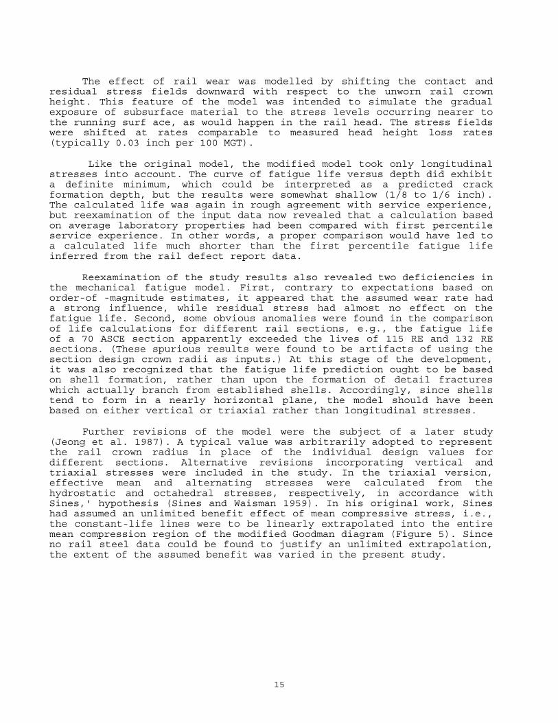
Table 4 summarizes the model validation. The model predictions have been adjusted by an empirically determined factor to reflect the effect of stress sequence on crack growth. Like the fatigue life model discussed earlier, the present LEFM model does not account for the effect of prior stress cycles on the crack growth rate in later cycles. The effect was determined by performing crack growth tests on laboratory specimens of rail steel under well controlled conditions, with a stress spectrum simulating the typical sequence which would occur during repeated passages of the FAST consist (Journet and Pelloux 1987; Journet and Pelloux 1988). The life adjustment factor was determined by comparing LEFM predictions with the laboratory test results. This factor was then applied to the detail fracture model.

The detail fracture model was used to study the sensitivity of crack growth life to variations in track construction, operational, and environmental factors (Orringer et al. 1988). For the purpose of the study, the crack growth life was arbitrarily defined to be the tonnage required to grow the detail fracture model from 10 to 80 %HA.7

7 There is some basis for these limits: 10 %HA is a reasonable estimate of the detectable size defined earlier (see also discussion in Section 2.2); and field experience suggests that detail fractures can routinely survive to 80 %HA in average service environments.

23

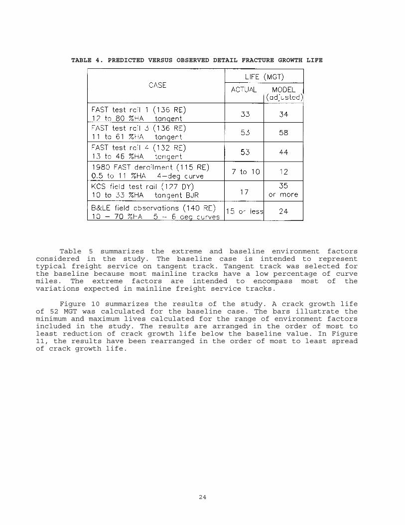
TABLE 4. PREDICTED VERSUS OBSERVED DETAIL FRACTURE GROWTH LIFE

Table 5 summarizes the extreme and baseline environment factors considered in the study. The baseline case is intended to represent typical freight service on tangent track. Tangent track was selected for the baseline because most mainline tracks have a low percentage of curve miles. The extreme factors are intended to encompass most of the variations expected in mainline freight service tracks.

Figure 10 summarizes the results of the study. A crack growth life of 52 MGT was calculated for the baseline case. The bars illustrate the minimum and maximum lives calculated for the range of environment factors included in the study. The results are arranged in the order of most to least reduction of crack growth life below the baseline value. In Figure 11, the results have been rearranged in the order of most to least spread of crack growth life.

24

TABLE 5. FACTORS AFFECTING DETAIL FRACTURE GROWTH

FIGURE 10. POTENTIALS FOR REDUCTION OF DETAIL FRACTURE LIFE

25

FIGURE 11. POTENTIALS FOR VARIATION OF DETAIL FRACTURE LIFE

It is apparent from the foregoing results that detail fracture crack growth lives can be expected to vary from a few MGT to more than 100 MGT over the range of typical conditions found in mainline freight service. Moreover, the most influential factors are those which are not under the immediate control of the track engineer. These observations suggest two important conclusions about the scheduling of rail tests. First, the test frequency should be varied to account for differences in annual tonnage carried by different lines. Second, allowance should be made for schedule flexibility to respond to changing service conditions, but in a manner which does not overburden the track engineer with consideration of too much detail.

Bolt hole cracks and vertical split heads have also been studied, but their crack growth properties have not been characterized as thoroughly as those of the detail fracture. No evidence has been found to indicate that these defects have safe lives much longer or shorter than the range of detail fracture life in typical service conditions.

An early study of bolt hole cracks focused on preventive maintenance by application of cold work to the bolt hole surface (Lindh et al. 1977; Lindh et al. 1979). The hole diameter is expanded by a tapered oversize mandrel, which is drawn through while a thin metal sleeve protects the bolt hole surface from galling.

26

The rail web material surrounding the hole is forced into plastic hoop tension during the expansion and is left with residual hoop compression after the mandrel has been withdrawn.

Trials on U.S. railroads showed that cold expansion was effective when applied to bolt holes in good condition but difficult and unreliable when applied to out-of-round holes. The procedure never gained wide acceptance in the U.S. as a maintenance practice because of its variable effectiveness and labor-intensive character. Cold expansion has recently been adopted by British Rail, however, with an improved procedure in which the holes are first reamed to a uniform diameter with low run-out (Cannon 1989).

The first study of fatigue crack growth and fracture behavior of bolt hole cracks was undertaken by the present author circa 1980, in connection with a specific problem which one western railroad had encountered on one of its lines carrying a high percentage of 100-ton unit train traffic. The line had been upgraded from medium weight bolted-joint rail to heavy CWR a few years earlier. The upgrade had the unusual feature that the CWR strings were joined mechanically rather than with field welds. The rail was box-anchored to every tie for eight rail lengths from the joint and to every other tie thereafter. Each winter this line was subject to bolt failures and joint pull-aparts which would generally occur within a short time after the first rapid change from above to below freezing weather. Three years after the upgrade the onset of winter weather brought sudden bolt hole breaks as well as pull-aparts. Many of these rail failures originated from bolt hole cracks which were at or below the estimated detectable size. These problems became academic when the railroad replaced the joints with field welds circa 1983, but the study yielded some useful general insights.

Field observations and measurements were made by the author. The observations revealed a seasonal cycle of fretting fatigue which formed the bolt hole cracks and then accelerated their growth. In the summer, when the rail-end gaps were closed, the bolt shanks were brought into bearing on the bolt hole surfaces of the rail webs at positions away from the rail ends (see Figure 12), and the fretting action was induced by train loads. When the rail-end gaps opened in the winter, the bolt shanks would bear toward the rail ends, placing the cracked part of the rail web under static tension. The combination of alternating web shear from the train loads and the static tension was sufficient to accelerate the rate of growth of the crack and, in extreme cases of cold-weather tension, to exceed the fracture strength at small critical crack sizes.

27

FIGURE 12. “WINTER BOLT HOLE CRACK” MECHANISM

The dimensions of several joints were measured in situ both as found and after disassembly. The measurements were compared with design tolerances to reconstruct the state of bearing between the bolts and bolt holes. For the typical joint, the results demonstrated that the fretting contacts had been concentrated on the field sides of the bolt holes in one rail and the gage sides in the other. These conditions suggest lateral loading and are also consistent with the corner-crack origins generally observed for bolt hole cracks.

One winter bolt hole crack which had grown to medium size before rail failure, and which had been removed from track to the laboratory before rust or field damage obscured the crack surface features, was found to possess a ridged surface similar to but much less pronounced than the ridges observed on the surfaces of the FAST test detail fractures. Similar ridges were produced in a laboratory experiment in which the test specimen was subjected to cyclic stresses with occasional changes in the orientation of the principal tensile stress (Mayville and Hilton 1984). The laboratory test simulated a bolt hole crack stress environment consisting of alternating web shear from train loads and a diurnal tension cycle from bolt bearing.

While mechanical joints between CWR strings are no longer of practical concern, bolt-bearing tension can be expected in other situations. Bonded insulated joints must still be used to divide signal blocks in CWR. The bolts and rail web bolt holes in these joints can become subject to severe bolt bearing effects if the bond fails. Some bolt-bearing tension can also be expected in poorly maintained bolted-joint rail at locations where locomotive tractions induce rail running.

28

Strain energy density and LEFM models have been used to estimate the growth lives of bolt hole cracks under assumed conditions of constant-weight axle loading and moderate bolt-bearing tension (Sih and Tzou 1985; Mayville et al. in press). As a part of the LEFM study, crack formation life was also estimated, with the results suggesting that fretting action would be required to form a bolt hole crack within the service life of the rail. The estimated lives ranged from about 5 to 30 MGT, but the calculations did not correspond to well defined safe crack size limits, nor were the models validated by comparison with field test results.

After the successful conclusion of the detail fracture experiment on the FAST track (Orringer, Morris, and Jeong 1986), a similar test to characterize bolt hole crack growth rates was attempted. Unfortunately, the only rails containing service-formed bolt hole cracks which could be obtained from revenue track at the time were found to be unsuitable for installation in the FAST track.

The Transportation Test Center was later able to identify ten bolt hole cracks which had formed in the FAST track; these defects were left undisturbed and were ultrasonically monitored over 50 MGT during the 100-ton phase of FAST operations. Seven of the ten defects were small corner cracks when found and remained in the corner-crack stage for the entire observation period. The eighth was found as a corner crack of about 0.4 inch radius and grew to a through crack about 0.8 inch long. The last two defects were found as through cracks respectively 1.5 and 2.25 inches long; these grew to lengths of 1.65 and 2.54 inches during the observation period. These test rates of growth are slower than the rates predicted by the fracture mechanics analyses.

In another test, the 100-ton FAST consist was run over a specially instrumented joint at speeds of 15 and 45 mph to collect dynamic load data. The loads were measured by means of strain gage bridges applied to the joint bars, measuring vertical bending and statically calibrated to vertical load. The joint setup was varied between train passes to investigate combinations of rail-end gap (0, 1/4, or 1/2 inch), height mismatch (0, 1/8, or 3/16 inch) with the receiving rail high8, and bolts tight or loose. Peak dynamic loads from 1.5 to 4 times the static vertical wheel load were measured. Generally speaking, the peak loads tended to increase as the gap, height mismatch, and train speed increased, although the trends were not uniform. However, the expected trend to larger loads with loose (as opposed to tight) bolts was not observed.

8 The quoted conditions are for the unloaded state. The mismatch conditions under load deviated from the static conditions due to dynamic rail-end dip and batter.

29

Vertical split heads (VSH) have traditionally been of great concern to track engineers because of the wide variety of lengths at which these defects have been initially detected. While rail tests find many VSH defects at lengths of 6 to 12 inches, initial discoveries at lengths of several feet are not uncommon. This situation has given rise to perceptions that VSH rail failure might be uncontrollable because of rapid or erratic crack growth and/or unreliable detection.

The behavior of VSH defects has not been studied by means of either fracture mechanics models or field tests. In spite of the lack of quantitative results for growth rates, however, some important qualitative results have been obtained from examinations of VSH defects which were broken open in the laboratory (R.A. Mayville, Arthur D. Little, Inc., unpublished, ref. nos. 55236 and 89674). Metallographic study of the crack surfaces generally revealed the presence of inclusion stringers or other microstructure anomalies distributed over the entire length of the defect. Conversely, areas on the same plane but outside the length of the defect were generally found to be free of stringers and to have normal microstructure. The height of the defect appeared to have increased at a slow fatigue rate of growth. The top and bottom crack fronts of a typical VSH would generally propagate along paths curving toward the rail center plane and the gage side head-web fillet, respectively. Defects which were well into this growth stage were also observed to have opened as the gage side of the rail head was gradually separating from the rest of the rail.

These metallographic observations suggest that the typical VSH grows lengthwise in rapid erratic jumps until all of the contiguous areas of stringer or poor microstructure have been encompassed. The wide range of detected VSH lengths is thus not surprising, nor should this range be a cause for undue concern. It appears that further growth in the vertical direction is required before the risk of rail failure becomes significant. The vertical growth appears to occur by means of a slow fatigue mechanism. The safe growth life should be of the same order as detail fracture life, since the fatigue and residual stresses which would drive VSH growth are of the same order as the stresses which make detail fractures grow.

30

2.2 Rail Testing

Railroads in the U.S. have been testing their rail to find defects in service for about 70 years. A rise in the incidence of service breaks in the late 1920s, following a decade of heavy rail system use, spurred the initial application of continuous search concepts to the maintenance of rail integrity. Magnetic induction was the first search method to be successfully applied and remained the primary method for about 40 years.9

The ultrasonic method came into widespread use in the early 1960s and is the most common technique today, although magnetic induction testing still plays an important role. Details of these methods and the history of their development have been summarized elsewhere (Sperry Rail Service 1964; Orringer and Ceccon 1980) and will not be repeated here.

Even within the technology of ultrasonic detection, a wide variety of procedures can be found in use in today I s fleets of rail test vehicles. The variations include probe positioning method (sled or wheel), beam entry angle, flaw indication method (transmission loss or reflection), and type of presentation (B or C scan). Different railroads have implemented different procedures in their own fleets of rail test vehicles. Some tracks are subjected to different procedures from a combination of tests by railroad-owned test cars and hired cars with different ultrasonic as well as magnetic induction equipment.

In the light of the fact that many different procedures are used on many different tracks, it should not be surprising that the performance of rail flaw detection equipment is extremely difficult to quantify. The situation is further complicated by differences in the skills of the test car operators and the impossibility (in practice) of making a thorough comparison of detections with the actual f law content of rail in service at the time of a test.10 Therefore, only rough estimates of rail test performance can be made from service data.

9 It is interesting to observe that the railroads began to test rail shortly after the first conceptualization of a sharp crack as a strength-reducing agent (Griffith 1920) and well ahead of the beginning of fracture mechanics as an engineering discipline (Irwin 1964).

10 Such evaluations of nondestructive inspection methods have been made in the laboratory, on parts production lines, and in maintenance shops. To do so, however, requires the determination of actual flaw content by means of an independent method much more sensitive (i.e., able to detect much smaller defects) than the method being evaluated. The independent method usually requires some degree of destruction of the articles being inspected, an option which is not available for rails still in service.

31

These estimates cannot isolate equipment performance from operator effects and the "opportunity factor". The opportunity factor comes into play when service and detected defect rates are compared to estimate detection probabilities. A given service defect may have been genuinely missed by the preceding test, or it may have simply been too small to find at the time of the test (lack of opportunity). Whether the opportunity existed or not depends on when the defect was formed, what its rate of growth was, and how frequently the track was tested.

Under these circumstances, the only quantitative results which can be obtained on flaw detection performance are rough estimates of net detection efficiency, including the skill and opportunity factors, averaged over an ensemble of track conditions, annual tonnages, test frequencies and procedures, and defect types and sizes. This type of estimate has been made from several samples of annual summaries of railroad defect reports. Annual summaries are better for this purpose than individual track test reports because annualized data tends to average the skill and opportunity factors. Test procedure variations, seasonal frequency changes, and defect characteristics are similarly averaged. Unfortunately, the annual statistics are usually reported at the division or railroad level, precluding any chance to empirically observe the effects of defect occurrence rate, test frequency, and annual tonnage on net detection efficiency.

In spite of these handicaps, some useful results have been obtained from the annual data. With the practices in use over the past 15 years, rail tests have generally been able to find from 50 to 90 percent of the total defects discovered. The 50 percent figure is not typical of most current mainline track but represents performance on older, poorly maintained bolted-joint rail, where about half the defects are bolt hole cracks. Conversely, rail tests typically find 80 to 90 percent of the defects in well maintained CWR, where detail fractures dominate the defect population.

One important performance factor which is masked by the averaging effects imbedded in the field data is the detectable defect size. Establishing the safe crack growth life for a given defect type requires a definition of the detectable size (see Section 2.1.2). However, all such definitions are imprecise because defects of the same type and size can be detected or missed on account of physical differences other than size. Therefore, the probability of detection as a function of defect size must be considered when a detectable size is chosen, but this function cannot be extracted from field data. Instead, a model must be constructed and correlated with the net detection probabilities which can be estimated from field experience.

32

2.2.1 Detection model

For a given type of defect, detection performance can be conceptually modeled as a detection probability function, p(A), where A represents the defect size. The function p(A) represents the percentage of detections expected from testing a large number of defects of size A. One intuitively expects the detection probability to rise with increasing defect size and to approach 1 (i.e., 100% detection) for large sizes, as suggested by the schematic illustration in Figure 13. The figure also illustrates the meaning of the term "detectable size" mentioned in section 2.1.2, namely: a smaller size A1 with a small but finite detection probability.

FIGURE 13. DETECTION PERFORMANCE CURVE

The relation between detection performance and net detection efficiency is most easily illustrated by the following simple example. Assume that the detectable size corresponds to p(Al) ≅ 0 and that the defect population is distributed among different sizes by the probability density function f(A), where f(A)∆A represents the percentage of defects having sizes between A and A+ ∆ A . Assume further that the distribution function is truncated to f(A) = 0 for A > Acr and renormalized, and suppose that the net detection efficiency for a single test is sought. The net detection efficiency is then the same as the weighted average detection probability obtained from the performance curve and the defect size distribution:

33

2

1

( ) ( )A

net avA

P P p A f A d= = ∫ A

]

(5)

This process of averaging over the defect size distribution accounts for the opportunity factor.

Application of these concepts to rail testing requires some modifications to account for the effects of repeated tests on a changing defect population. Under these circumstances, net detection efficiency cannot be equated to average detection probability, as it was for a single test. Also, practical applications require assumptions about the physical characteristics and size distribution of the defect population.

Consider the effect of two tests on one defect. The defect is assumed to grow in the interval, from size A1 at the time of the first test to size A2 at the second. If the test times and defect sizes are sufficiently separated, then they can be assumed to be uncorrelated, and the combined detection probability is given by:

[ ][12 1 21 1 ( ) 1 ( )p p A p A= − − − (6)

Equation (6) is the well known expression for the total probability of two events with independent individual probabilities. The hypothesis of independence cannot be proved for the rail tests but is reasonable if the effects of metal fatigue, change of rail surf ace condition, and/or changing seasonal factors intervene between the tests. Under these conditions, p12 represents the percentage of detections which would be expected if a large number of defects were all tested at size A1 and these not detected were tested again at size A2.

The effect of repeated testing on a population of defects can be estimated by combining models of their formation and growth behavior to generate the size distribution function. For example, the cumulative percentage of rails that have formed defects after N MGT of service can be represented by an empirical Weibull cumulative distribution (see eq. (1) in Section 2.1.1) The corresponding Weibull density function is given by:

( )1

/( ) NNf N eαα

βα

αβ

−−= (7)

and means that f(N)∆N represents the percentage of rails which form defects between N and N+∆N MGT. An average defect size versus tonnage

34

growth curve can then be used to define a sequence of sizes A1, A2, A3, … such that equal tonnages ∆N are required to grow a defect from one size to the next. If

( ) ( )1 1 1 2 1( ) ( )f A A f A A A f N N∆ = − = ∆ (8)

represents the defects which most recently became detectable, then the distribution of larger defects ( Ai ≤ A ≤ Ai+1 ; i ≥ 2 ) is given by:

( ) ( )i i if A A f N i N N∆ = − ∆ ∆ (9)

Equations (8) and (9) would introduce some error if f(N) strictly represented the tonnage for defect formation. However, the empirical Weibull life distributions discussed in Section 2.1.1 actually represent the tonnage to formation plus growth to detectable size and are, therefore, consistent with eqs. (8) and (9).

Let pi be the average detection probability for the ith size range.

If the ranges ∆Ai are small compared to the complete safe crack growth range Acr-A1 , the averages can be estimated with acceptable accuracy by either of the following formulae:

1

2i i

iA Ap p ++⎛ ⎞= ⎜ ⎟

⎝ ⎠ (10a)

( ) ( )12i ip p A p A += +1i⎡ ⎤⎣ ⎦ (10b)

where p(A) is the detection performance curve (Figure 13).

The probability model can be applied to estimate net detection efficiency for multiple tests as follows. For example, suppose that two tests are performed per safe crack growth life. Divide the detectable defect population into 2m equal-tonnage size intervals ( Ai, Ai+1 ) define i = 1, 2, …, m as the first half and i = m+1, m+2, …, 2m as the second half of the population. Note that each half will be tested twice: once when it occupies the first m size ranges and once when it occupies the second m size ranges. The interval between these tests satisfies the criterion of reasonable separation. Therefore, the two-event detection probability formula applies to both halves of the population, and the net detection efficiency is given by:

[ ] ( ) (1

( ) ( ) 1 1 1m

net i i i m i m i i mi

P f A A f A A p p+ + +=

= ∆ + ∆ − − − )⎡ ⎤⎣ ⎦∑ (11)

35

2.2.2 Correlation with field experience

Precise experiments to measure detection equipment performance are difficult to conduct, even under well controlled laboratory conditions, and quantitative results are virtually impossible to obtain for rail testing under field conditions. Therefore, the modeling of rail test equipment performance has been limited to sensitivity studies (D.D. Davis et al. 1987; Orringer 1988) and correlation with field experience. The correlation was limited to a comparison based on general knowledge of detail fracture detectability under current U.S. rail test practices and on the provisions of an equipment performance specification recently adopted by the Canadian Pacific Railroad. The correlation study has not been previously published11 and will, therefore, be recounted here.

Reflections of ultrasonic beams introduced into the rail head via the running surface at angles between 35 and 70 degrees from the vertical are the primary means of detecting detail fractures. The best performance is obtained when the probe beam is aligned along the rail with the target defect. Even in this case, the presence of a very small detail fracture may be masked by the overlying shell (Figure 14). In practice, the detection performance can be degraded by beam offset, which is a function of the varying lateral position of the probe carrier on the running surface, and by minor surface roughness (e.g., in tests of rail from which the surface oxides have not been polished 'by recent traffic). The signal return display also requires interpretation to differentiate between shells and detail fractures, a factor which brings operator skill into the performance picture.

FIGURE 14. MASKING EFFECT OF SHELL

11 Orringer, 0., "Preliminary Evaluation of CP Rail Test Performance Specification," DOT Transportation Systems Center, Cambridge, MA, memorandum to R.J. McCown, FRA Office of Research and Development (RRS-31), March 30, 1987 (unpublished).

36

When detected, detail fractures are verified and classified by means of test procedures based on hand-held ultrasonic probes. The defects are classified as small (less than 20 %HA), medium (20 to 40 %HA), or large (more than 40 %HA) in accordance with the current Track Safety Standards.

Independent vendors of rail test services are generally willing to guarantee the detection of medium and large detail fractures but are often reluctant to extend the guarantee to small detail fractures. Conversely, some experienced rail test operators employed by railroads do not hesitate to express confidence in their own ability to find detail fractures as small as 5 %HA. The vendors have equally experienced operators, and the apparent contrast in confidence levels reflects the physical problems which tend to reduce detection performance for small detail fractures. Conversations with several experienced operators and rail test managers suggest that detections of about one out of three 10 %HA detail fractures is expected, and it appears reasonable to assume that 5 %HA is the lower limit for detection.

A detection performance model which represents the foregoing characteristics is defined by:

(12) ( ) ( )*

1 15 /( ) 1 A A A Ap A e− − −= −

where A1 = 5 %HA and A* = 75 %HA. Figure 15 illustrates the eq. (12) detection performance curve.

FIGURE 15. DETAIL FRACTURE DETECTION PERFORMANCE MODEL

37

The model can be judged by comparison with a Canadian Pacific Railroad specification for rail test performance. The specification was adopted circa 1986 as a requirement which must be met by all vendors of rail testing services to the CP. The provisions governing detail fractures require minimum detection performances for the small, medium, and large size categories. Table 6 compares these requirements with the performance inferred from the model by taking unweighted averages of eq. (12) over the three size ranges. The comparison suggests that the model is in reasonable agreement with the CP distillation of its own experience.

TABLE 6. COMPARISON OF DETAIL FRACTURE DETECTION PERFORMANCE MODEL WITH CP SPECIFICATION

How well does the model reflect detection performance on U.S. railroads? No written requirements equivalent to the CP specification are available for comparison, but net detection efficiency as predicted by the model can be compared with the field experience extracted from railroad annual defect summary reports. Such a prediction was made in accordance with the procedure outlined in Section 2.2.1, using α = 3 and β = 2,000 MGT in the Weibull model for defect formation (Section 2.1.1) and a representative average growth curve based on the results of the FAST test of detail fractures (Section 2.1.2). Table 7 summarizes the division of the growth curve into 2m = 10 size ranges. Average growth through each range requires 5 MGT, i.e., the safe crack growth life from 10 %HA to 80 %HA is 50 MGT. The table also gives the average detection probabilities for the size ranges, as obtained from eq. (10b) and (12).

38

TABLE 7. DETECT SIZE RANGES AND DETECTION PROBABILITIES

(5 MGT PER RANGE)

Numerous high tonnage lines in the U.S. have annual tonnages of about 50 MGT and are tested twice per year. Detail fractures tend to dominate the defect populations on these lines, and the actual detection performance on these lines is well represented by the annual summary statistics. Therefore, a prediction based on eq. (11) with m = 5 provides a reasonable basis for comparing the model to the field experience. Cases with N = 105 MGT and N = 505 MGT were calculated to represent track at early and mid-life rail ages, respectively. The model gave Pnet predictions of 0.88 and 0.90 for these two cases, results which agree well with the field experience of 80 to 90 percent detection reliability on modern CWR lines where detail fractures make up the major proportion of the defect population.

39

2.3 Maintenance of Rail Integrity

Maintaining the integrity of rail means keeping the rate of service defects down to a level at which the risk of derailment from rail failure is acceptably low. What is meant, however, by “acceptably low”? The definition is ultimately based on a posteriori social decisions which lie outside the province of engineering. In the present work, the average status quo is assumed to be the product of these decisions and is accepted as a basis for the proposed test scheduling guidelines. It is further assumed that national average performance figures from the past decade reflect the acceptable level of risk.

What are the relevant performance figures? It was mentioned earlier that the national average rate of defects detected by rail test lies between 0.4 and 0.8 per track mile (Thomas 1985), and the recent trend has been toward the lower figure. Extrapolation from these rates, based on the 80 to 90 percent net detection efficiency commonly realized on modern track, suggests that the corresponding service defect rate ranges from 0.04 to 0.2 per track mile. The middle of this range, i.e., about 0.1 service defect per track mile, is therefore an appropriate baseline.

This baseline can also be compared with other national average figures and study results. The national average rate of derailments caused by rail failures is on the order of one derailment per hundred service defects (Orringer and Bush 1983). In other words, at a service defect rate of 0.1 per track mile, one may expect one derailment per thousand track miles in each interval between tests. Since test intervals tend to average between 20 and 25 MGT on medium tonnage lines12, 0.1 service defect per track mile roughly equates to 4 to 5 service defects per billion gross ton miles (BGTM), or about ten times the rate per BGTM observed in detailed studies of several lines belonging to four railroads (Orringer and Bush 1983).13

The proposed guideline for scheduling rail tests is based on a performance target of 0.1 service defect per track mile between tests. The guideline is further based on the empirical Weibull model for defect formation and on a representative detail fracture safe crack growth life of 40 MGT. The selection of 40 MGT rather than the 50 MGT baseline shown in Figures 10 and 11 is intentionally conservative in order to reflect the effects of revenue track conditions together with a small proportion of low degree curves. The guideline is developed from these defect formation and growth characteristics, together with the detection

12 Strictly speaking, these test interval figures apply to single-track territory, which tends to drive the test schedule for the entire line.

13 The study failed to find a strong correlation between service defect and derailment rates, but a trend was indicated.

40

performance model defined by eq. (12). The ratio of service to detected defects is a convenient parameter for the purpose of developing the guideline. In terms of net detection efficiency, this ratio is given by:

1 net

net

PSD P

−= (13)

where S is the rate of service defects per track mile between tests and D is the rate of detected defects per track mile from the most recent test.14 The shaded region in Figure 16 is the calculated S/D ratio. The upper bound reflects the results of the analysis procedure outlined in Section 2.2.2; the lower bound corresponds to a simplified analysis which does not account for defect growth between tests. The figure also shows a straight-line approximation of the upper bound. The approximation is introduced for arithmetical convenience and is given by:

( )0.014 10S ND

= ∆ − (14)

where ∆N is the interval between tests, expressed in MGT.

FIGURE 16. RATIO OF SERVICE TO DETECTED DEFECTS

14 D includes all defect types except engine burns or service bent rails. Any defects detected by a previous test but remaining in track under protection are also excluded.

41

For a standard track mile (273 lengths of 39-foot rail), the expected population of defects which reach detectable size between one test and the next is:

(15) ( ) 273 ( )S D N f N N+ ∆ = ∆

where f(N)∆N is an appropriate empirical Weibull life distribution.15 The expected rate of service defects per track mile between tests can then be approximated by:

1

/

273 ( )

1S D

f N NS N ∆∆ ≅+

(16)

where S/D is obtained from eq. (14). Setting S∆N = 0.1 (the performance target) and solving eq. (16) for ∆N then yields an idealized scheduling program as a function of cumulative tonnage, N. Figure 17 plots two such results based on the empirical Weibull life distributions: α=3 and β=1,000 MGT to represent the FAST track; and α=3 and β=2,000 MGT to represent track carrying average mixed freight (AMF) service. Both programs are arbitrarily restricted to ∆N ≤ 40 MGT in order to provide at least one test per average safe crack growth life.

FIGURE 17. IDEALIZED SCEDULING PROGRAMS

The curves in Figure 17 illustrate the fundamental effect of exposure to risk. Exposure to the risk of rail failure and derailment rises as the rate of defect formation rises with accumulating tonnage.

15 The expectation assumes no more than one defect per rail, which closely corresponds to the reporting conventions from which the empirical life distributions are derived.

42

To keep the risk at the acceptable level ( S∆N = 0.1 ) requires more frequent testing (i.e., shorter intervals between tests) as tonnage accumulates.

While tonnage-based scheduling programs are useful for illustrating general principles, they are not convenient to apply. In practice, the defect formation rate on an actual line is not known a priori and may fluctuate as rail is renewed on parts of the line. If the programs are replotted versus total defect rate S + D, however, the characteristic life P is factored out, and the two programs fall on a single master curve (Figure 18). A track engineer could use this curve as indicated by the arrows, reading up from the current actual total defect rate and then across to find the interval to the next test.

FIGURE 18. MASTER SCHEDULING CURVE

Another view of the master curve's effect is obtained by comparing its performance target with the service defect rates which would result from constant-frequency test schedules. Figure 19 illustrates comparisons based on the FAST and AMF life distribution models, assuming that the tests are performed at 20 MGT intervals. It is apparent that the constant-frequency schedules over-control rail integrity at low accumulated tonnage and under-control at high tonnage. Averaging the service defect rate over the 1,080 MGT AMF rail life shown in the figure gives S∆N = 0.093. The FAST case represents heavy haul service, where one might expect the rail to be cascaded to a less demanding service at about 400 MGT. Averaging to the 400 MGT point gives S∆N = 0.117. These values closely bracket the master curve performance target, which thus appears to well reflect the average of current practices.

Rail tests could be scheduled by means of the master curve alone if the defect growth behavior and detection performance were always as defined by the models used to generate the curve. However, these models are only averages at best, and in practice even the averages may vary from one line and/or time to another. Following the master curve under such conditions will cause the performance figure S∆N to vary, requiring some additional means of schedule adjustment.

43

FIGURE 19. DEPENDENCE OF SERVICE DEFECT RATE ON TEST SCHEDULE

The model parameters were varied to illustrate the effects of two types of deviation. First, a hypothetical transient effect of service or maintenance changes was simulated by doubling the model defect formation rate. Second, a degradation in the actual defect performance was simulated by replacing eq. (14) with:

( )0.015 5S ND

= ∆ − (17)

Figure 20 compares the S/D ratio used to derive the master curve with the assumed degraded ratio.

F I G U R E 2 0 . V A R I A T I O N O F D E T E C T I O N P E R F O R M A N C E

Figure 21 summarizes the examples by plotting the service defect rate as a function of the interval between tests. In each case, total tonnage accumulates in the direction indicated by the arrow. Current practice, as represented by the constant 20 MGT interval, is included for comparison. The curve labelled TRANSIENT shows the effect of doubling the defect formation rate. In this case, the performance target is

44

temporarily exceeded by about 10 percent, but the test interval adjustments based on the master curve eventually compensate. Conversely, the deviation of detection performance (curve marked DEGRADED) causes the master curve compensation to lag further and further behind the actual situation, requiring additional means of adjustment. A similar effect would be created by consistent deviations in the rate of defect growth, since detection performance depends in part on the safe crack growth life.

FIGURE 21. EFFECT OF BEHAVIOR DEVIATIONS ON PERFORMANCE

45

3. TEST SCHEDULING GUIDE

A practical test scheduling guide was developed from the master curve in two steps. First, the detection performance model was used to derive a procedure for revising the test interval to compensate for behavior deviations (Section 3.1). Second, the master curve and adjustment procedure were integrated into a combined graphical format to make the guide easier to apply (Section 3.2). Some examples are presented in Section 3.3 to show how the guide is used.

3.1 Adjustment Procedure

The basic idea behind the adjustment procedure is that deviations in defect formation or growth rates or in detection performance will be reflected by a deviation in the service defect rate. In the present context, "deviation" refers to departures from the baseline assumptions: (1) a unimodal distribution of time to defect formation with Weibull shape factor α= 3; (2) a safe crack growth life averaging 40 MGT with rates characteristic for detail fractures; (3) detection performance as defined by eq. (14); and (4) S∆N = 0.1 service defect per track mile between tests as the performance target.

Deviations below the target reduce risk and, therefore, are not a cause for concern and do not require test interval adjustment beyond the guideline provided by the master curve. Deviations above the target increase risk and do require adjustment. The interval to the next test must then be decreased, with respect to the value suggested by the master curve, in order to bring the service defect rate back down toward the target.

The adjustment procedure is bases on the detection performance model. Suppose that the interval Ƅ between the two most recent inspections has produced a service defect rate SƄ > 0.1, and assume that the underlying behavior factors will not change to any great extent during the next interval. It then follows from eq. (14) that the shorter interval defined by:

* 0.10.014

S NN N ∆ −∆ = ∆ −%

% (18)

should meet the performance target where Ƅ is the actual previous interval.

The first trial adjustment procedure was simply to replace ∆N (from the master curve) by ∆N*, but a preliminary study showed that this procedure led quickly to over-control in most cases. The adjustment was then damped by means of the following modified procedure: (1) replace ∆N by (∆N+∆N*)/2 if the service defect rate target is exceeded; (2) the next interval shall, however, not be less than 3/4 nor more than 3/2 of the preceding interval; and (3) the result of calculations (1) and (2) shall be rounded to the nearest two MGT. An extensive simulation study of the modified guide showed that it was adequately damped yet still able to compensate for most kinds of deviation (see Section 4).

46

3.2 Performance Chart

The arithmetical form of the adjustment procedure was deemed to be inconvenient to apply and also appeared to be a potential source of error from misunderstanding. Therefore, a graphical equivalent was sought for use in conjunction with the master curve. Simultaneously, the master curve was extended to cover total defect rates well beyond those expected in revenue track, in order to reduce the potential for ambiguity in applications.

It was not possible to convert the entire adjustment procedure to a convenient graphical form. However, the extended master curve and the averaging rule (∆N+∆N*)/2 could be combined on a single nomogram type graph. Figure 22 illustrates this performance chart.

The master curve appears at the left side, with a change of scale in the extended region in order to fit the entire nomogram on a single sheet of paper. Reading from the total defect rate down to the curve and then across to the right margin of the box marks the ∆N value.

The diagonals in the right hand box are guidelines equivalent to eq. (18). This half of the chart is used in three steps as follows. First, read down from the service defect rate. Second, start at the right hand margin from the tonnage in the preceding interval and read diagonally down, parallel to the guidelines. Steps one and two will define a point of intersection. Third, read across from the intersection to the left margin of the box to mark the ∆N* value.

After the ∆N and ∆N* values have been marked, the average is taken by ruling a straight line connecting the two points. The intersection of that line with the center vertical scale then indicates the tonnage interval to the next test. The results can be read to the nearest two MGT and subsequently checked for compliance with the “3/4 -- 3/2” rule.

3.3 Example Applications

The following hypothetical example illustrates the steps described in the preceding section. On a line segment containing 35 track miles, the most recent rail test resulted in the detection of 14 defects. The interval between the most recent and preceding tests was 34 MGT. In that interval, 5 service defects were reported.

The defect rates must be calculated before the guide can be applied. Dividing the defects counts by the track mileage yields the rates:

47

FIGURE 22. RAIL TEST SCHEDULING PERFORMANCE CHART

48

SERVICE DEFECT RATE = 5/35 = 0.14 DETECTED DEFECT RATE = 14/35 = 0.40

TOTAL DEFECT RATE = 0.54

Figure 23 illustrates the application. The master curve graph is entered from the top at the total defect rate of 0.54 (point A). The graph is read down from A to find point B on the master curve, and then across to the right margin where point C is marked.

The adjustment graph is now prepared for use. The service defect rate of 0.14 is marked at the top (point D), and a vertical line is ruled from that point. The last inspection interval of 34 MGT is marked at the right margin (point E), and a diagonal line parallel to the guides is ruled from that point. From the intersection of the vertical and diagonal lines (point F), the graph is read across to the left margin where point G is marked.

A straight line connecting points C and G completes the construction. This line intersects the center vertical scale at point H, which is read (to the nearest two MGT) as 28 MGT for the interval to the next test. Since 28 MGT is more than 3/4 of the preceding 34 MGT interval, the result can be accepted without further adjustment.

The remaining examples are also hypothetical cases but are close to some actual cases analyzed in trial applications made by a participating railroad. Most of the examples illustrate one or more extrapolation ambiguities encountered by the track engineer. Since extrapolation was not the intended procedure, the discussion focuses on the proper treatment of these cases.

Figure 24 illustrates an application to a 30-mile line segment with a 12 MGT test interval, 15 service defects (0.5 per mile) since the preceding test, and 36 detections (1.2 per mile) from the most recent test. In this case, the intersection point F would lie below the adjustment graph if the construction were extrapolated. The proper action is to take the bottom margin (zero MGT) as a limit for point G. This leads to a suggestion of 8 MGT for the interval to the next test. Since this result is less than 3/4 of the preceding interval, however, the next interval should be set at 9 MGT.

Figure 25 illustrates an application to a 10-mile line segment with a 14 MGT test interval, no service defects since the preceding test, and two detections (0.2 per mile) from the most recent test. Note that total defect rate of 0.2 per mile lies to the left of the master curve. This is the region in which the 40 MGT restriction is set (see Figure 18). Therefore, point c is simply located on the upper right corner of the graph. Also, no adjustment for deviation is required, since the service defect rate is less than 0.1 per mile. Therefore, the adjustment graph is simply read straight across at 14 MGT to establish point G. A result of

49

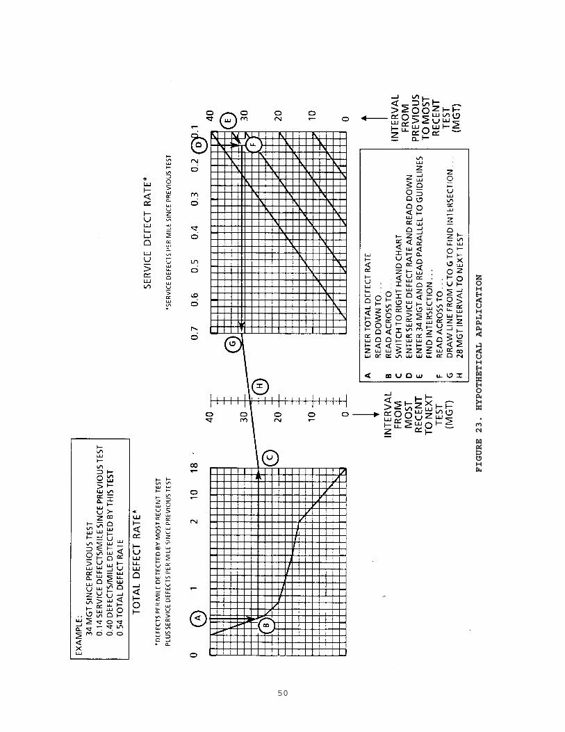
FIGURE 23. HYPOTHETICAL APPLICATION

50

FIGURE 24. PROCEDURE FOR OFF-SCALE ACJUSTMENT

51

FIGURE 25. EXAMPLE OF LOW DEFECT RATES

52

26 MGT is obtained from the chart; this exceeds 3/2 of the preceding interval, however, so the interval to the next test should be set at 21 MGT.

The final example to be discussed illustrates a modified procedure for dealing with annualized data, which is the usual record-keeping practice employed by the railroads. In this case, a 60-mile line segment carries 50 MGT annual tonnage and has recently been tested twice per year. In the most recent year, 19 service defects and 20 detected defects were reported.

To produce the proper defect rate numbers for the performance chart, the number of tests per year must be made a divisor together with the track mileage:

SERVICE DEFECT RATE = 19/60/2 = 0.16 DETECTED DEFECT RATE = 20/60/2 = 0.17 TOTAL DEFECT RATE = 0.33

Also, the tonnage to be entered on the adjustment graph is the annual tonnage divided by the number of tests per year (50/2 = 25 MGT).

Figure 26 illustrates the application. Completing the construction gives 30 MGT for the next interval, a result within 3/2 of the preceding average interval. In calendar terms, the result is equivalent to a little more than seven months to the next test. Seven-month intervals would be appropriate from a technical standpoint but could cause an accounting problem for the following calendar year, during which only one test would be performed. Therefore, additional procedures would still be required to credit the railroad for the actual interval.

53

FIGURE 26. APPLICATION BASED ON ANNUAL DATA

54

4. BEHAVIOR STUDIES

How well does the guide work? In theory it is supposed to provide for flexible scheduling of rail tests to compensate for changing circumstances, while controlling exposure to service defects. These aspects of the guide were investigated by means of a simulation study. The defect formation, growth, and detection models were altered in various ways to create simulated counts of detections and service defects. The simulation was coupled to the master curve (Figure 18) and the arithmetical adjustment rules (Section 3.1) to study the effects of the interaction between the scheduling guide and the simulated environment. Section 4.1 presents the results.

In theory the guide should also tend to reflect current practice. This aspect was studied by track engineers who made trial applications of the performance chart (Figure 22), using actual data taken from selected line segments on their railroads. The test intervals suggested by the chart were compared with the actual intervals being used by the railroads. Section 4.2 presents these results.

4.1 Simulation Studies

A statistically uniform line segment was simulated, except where specifically noted otherwise. In physical terms, the uniform property can be interpreted as: rail of common origin, section, and age; mostly tangent track with a small percentage of low-degree curves; uniform ballast and subgrade conditions; and single track with no traffic division points in the segment. Simulated defect formation rates were generated from the Weibull life distribution model, based on 273 rails per track mile. The length of the simulated segment did not enter into the calculations and was therefore undefined.

Each simulation started from newly re-railed track, with the first test performed at 100 MGT. Subsequent tests were assumed to be performed at intervals specified by the scheduling guide.16 The detection performance model (baseline or a variation) was used to calculate the detected defect rate for each test. The remainder of the defect rate was held over and added to the formation rate for the next interval, except that defects exceeding the assumed safe crack growth life were reassigned to the service defect rate. The minor reduction of defect rates due to defective rail replacement was not accounted for.

Figure 27 illustrates a simulation of an average mixed freight (AMF) line assumed to carry 40 MGT per year on rail with Weibull life parameters α = 3 and β = 2,000 MGT. The simulation was carried through 29 years of rail life.

16 The specified intervals were rounded to the nearest MGT, rather than the nearest two MGT prescribed for practical applications.

55

FIGURE 27. SIMULATION OF MEDIUM DENSITY AMF LINE

56

In the upper half of the figure, three plots illustrate different aspects of the simulated history. The left hand graph shows the cumulative number of rail tests as a function of accumulated tonnage and calendar years. The result of the guide is the curve labeled STRATEGY. The dashed line represents current practice: first test17 at the end of three calendar years and a constant interval of 20 MGT thereafter. The simulated test intervals are longer than 20 MGT for the first 13 years, about equal to 20 MGT over years 14 to 20, and shorter than 20 MGT from year 21 onward. The cumulative number of tests over the 29 year history is about equal to the number corresponding to current practice. The right hand graphs show the number of tests per year and the simulated annual defect rate.

The two plots in the lower half of the figure further illustrate the guide's performance. In the first plot, the master curve is reproduced in boldface, and the data points show the trend of test intervals specified by the guide. The data points in the second plot compare the simulated service defect rate history with the target of 0.1 per mile. The simulated performance is quite close to the ideal goal in this case, since the simulated environment does not deviate from the assumptions used to develop the guide.

Figure 28 illustrates a simulation of a heavy haul line carrying 100 MGT per year of 125-ton unit train traffic. In this case, the characteristic fatigue life has been reduced to β = 1,280 MGT. The average safe crack growth life has also been reduced from 40 to 32 MGT, represented by the apparent detection performance:18

( )0.0175 8S ND

= ∆ −

(19)

A six-year (600 MGT) history has been simulated, i.e., somewhat beyond the point at which economic considerations would probably dictate cascading the rail to less severe service. The guide again produces a trend of decreasing test intervals, with the total number equal to the number representing current practice.

Note that after an early lag19 the guide eventually tends to follow a path slightly below the master curve. This reflects the guide's self-adaptive character, i.e., it is seeking the path that would have been the

17 Other than the initial rail quality test performed shortly after rail is laid. The initial quality test is not counted in the simulation either.

18 Equation (19) is used only to calculate the simulated service and detected defect rates. Test interval adjustments are still calculated from eq. (18).

19 The lag is a side effect of the “3/4 -- 3/2” rule.

57

FIGURE 28. SIMULATION OF A HEAVY HAUL LINE

58

master curve, had the curve been derived from the degraded detection performance. The exposure tends to remain somewhat above the 0.1 per mile target and tends to oscillate, but it is still acceptable until near the end of the simulated history. For the last few tests (data points connected by dashed lines), the “3/4 -- 3/2” rule was intentionally suspended to show that the damping provided by this rule is essential to maintain rail integrity in the presence of moderate behavior deviations.

Table 8 summarizes seven additional simulations which were performed to study the reaction of the guide to several different kinds of deviation. The baseline case simulates a high density mixed freight (HDMF) line carrying 60 MGT per year with a somewhat reduced rail fatigue life (β = 1,420 MGT) but no deviations. The baseline simulation (Figure 29) produces results similar to the AMF case discussed earlier. Figures 30 through 35 illustrate the other simulations.

TABLE 8. SUMMARY OF HDMF SIMULATIONS

59

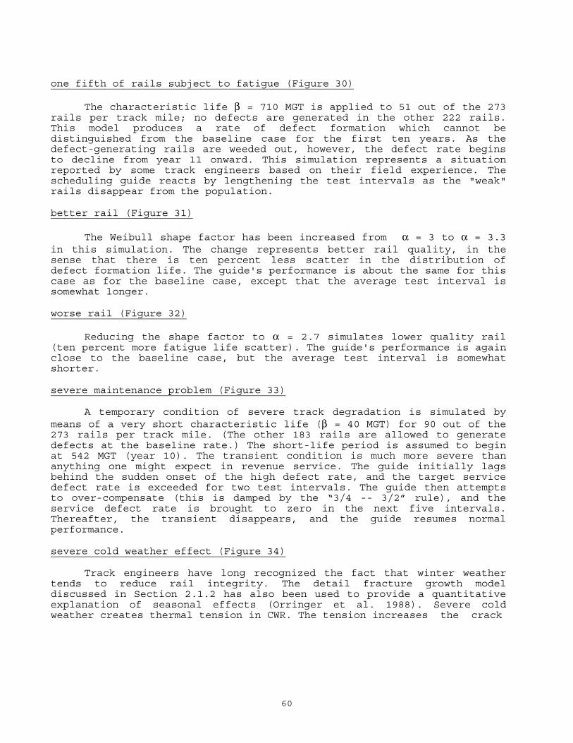
one fifth of rails subject to fatigue (Figure 30)

The characteristic life β = 710 MGT is applied to 51 out of the 273 rails per track mile; no defects are generated in the other 222 rails. This model produces a rate of defect formation which cannot be distinguished from the baseline case for the first ten years. As the defect-generating rails are weeded out, however, the defect rate begins to decline from year 11 onward. This simulation represents a situation reported by some track engineers based on their field experience. The scheduling guide reacts by lengthening the test intervals as the "weak" rails disappear from the population.

better rail (Figure 31)

The Weibull shape factor has been increased from α = 3 to α = 3.3 in this simulation. The change represents better rail quality, in the sense that there is ten percent less scatter in the distribution of defect formation life. The guide's performance is about the same for this case as for the baseline case, except that the average test interval is somewhat longer.

worse rail (Figure 32)

Reducing the shape factor to α = 2.7 simulates lower quality rail (ten percent more fatigue life scatter). The guide's performance is again close to the baseline case, but the average test interval is somewhat shorter.

severe maintenance problem (Figure 33)

A temporary condition of severe track degradation is simulated by means of a very short characteristic life (β = 40 MGT) for 90 out of the 273 rails per track mile. (The other 183 rails are allowed to generate defects at the baseline rate.) The short-life period is assumed to begin at 542 MGT (year 10). The transient condition is much more severe than anything one might expect in revenue service. The guide initially lags behind the sudden onset of the high defect rate, and the target service defect rate is exceeded for two test intervals. The guide then attempts to over-compensate (this is damped by the “3/4 -- 3/2” rule), and the service defect rate is brought to zero in the next five intervals. Thereafter, the transient disappears, and the guide resumes normal performance.

severe cold weather effect (Figure 34)

Track engineers have long recognized the fact that winter weather tends to reduce rail integrity. The detail fracture growth model discussed in Section 2.1.2 has also been used to provide a quantitative explanation of seasonal effects (Orringer et al. 1988). Severe cold weather creates thermal tension in CWR. The tension increases the crack

60

growth rate and decreases the critical size for detail fractures. Both effects tend to decrease safe crack growth life.

The seasonal effect is simulated by switching back and forth between the baseline and a deviation intended to represent the winter effect on detail fractures. The deviation is applied during the first two tenths and the last tenth of each year (roughly late November through mid March) and is defined by:

( )0.03 4 for 20 MGTS N ND

= ∆ − ∆ < (20a)

( )0.48 0.05 20 for 20 40 MGTN NSD

= + ∆ − ≤ ∆ ≤ (20b)

Equations (20a,b) simulate the apparent degradation of net detection efficiency for detail fractures which cause rail failure at a critical size of 30 %HA after a 20 MGT safe crack growth life.

The guide reacts by oscillating out of phase with the seasonal effect, viz: the high winter service defect rate leads to short test intervals during the warmer seasons, while the consequently low warm-weather rate allows long intervals during winter. The guide's performance might be judged barely acceptable up to year eight (480 MGT), but the increased exposure thereafter overwhelms the ability of the guide to compensate.

better test equipment (Figure 35)-

The effect of a modest improvement in rail test equipment has been simulated by decreasing the service/detected defect ratio to:

( )0.011 10S ND

= ∆ − (21)

Equation (21) represents a ten percent improvement in net detection efficiency with no change in the minimum detectable defect size. The guide reacts with a modest lengthening of the average interval between tests.

summary

Figure 36 summarizes the simulation study results. The different cases are compared in terms of the following performance statistics: average test interval; average number of tests per year; average service defect rate; and ±σ bounds20 on the service defect rate. The average

20 The bounds encompass 95 percent of the service defect rate performance data points.

61

62

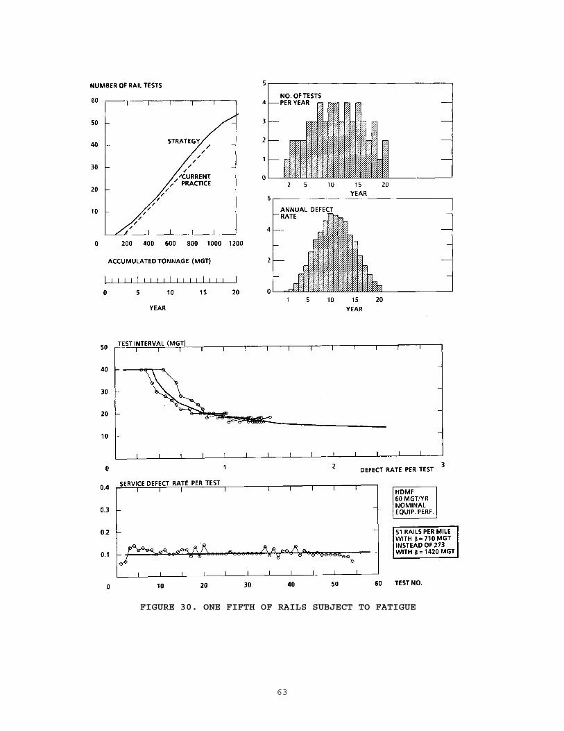
FIGURE 30. ONE FIFTH OF RAILS SUBJECT TO FATIGUE

63

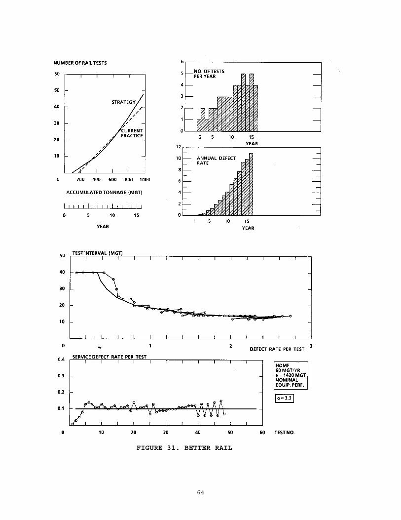
FIGURE 31. BETTER RAIL

64

65

FIGURE 32. WORSE RAIL

FIGURE 33. SEVERE MAINTENANCE PROBLEM

66

FIGURE 34. SEVERE COLD WEATHER EFFECT

67

FIGURE 35. BETTER TEST EQUIPMENT

68

interval ranges between 18 and 24 MGT. The average number of tests per year ranges between two and three except for the heavy haul line, which averages close to five. The service defect rates are, in general, tightly clustered around the 0.1 per mile target. The severe maintenance transient case leads to large but still acceptable scatter. However, the seasonal severe cold weather effect defeats the guide.

FIGURE 36. SUMMARY OF SIMULATION STUDY RESULTS

69

4.2 Railroad Studies

Track engineers of the Atchison, Topeka, and Santa Fe (ATSF), Southern Pacific (SP), and Union Pacific (UP) railroads investigated the practical aspects of the scheduling guide by making trial applications of the performance chart. The annual tonnages and defect reports for a recent year on representative line segments were used as inputs.21 In each case, a suggested test interval was obtained from the graphical construction procedure, but the "3/4 -- 3/2" rule was not applied. Each suggested interval was compared with the actual interval (s) used in the same year. The study results were forwarded to the Transportation Systems Center for review and further analysis.

The ATSF study focused on a southwestern division and included low-tonnage track for which neither the current federal standards nor the proposed guide would require rail testing. The railroad tests this trackage in accordance with its own policies, however, and the study thus provided a useful perspective on the practical limitations of a general guide.

ATSF tracks are inventoried by means of a state-of -the art computerized database which is linked with databases covering rail test results, service defect reports, and remedial actions. The track inventory is resolved down to tenths of a mile, generally to identify short stretches of unusual rail section, old rail, and/or changes between single and double track. The ATSF track engineers based their study on the existing breakdown, evaluating the guide on 81 identified segments ranging from 0.1 to 54.3 miles in length and 0.2 to 52 MGT in annual tonnage. The segments can be grouped into three general categories (Table 9): mainline single track carrying 52 MGT per year; other single track; and the one of the two tracks in double track territory. The study was performed to several-place precision on a computer; the present author has rounded the results to the nearest 0.5 MGT.

21 The ATSF and SP studies followed the procedure outlined earlier for working with annualized data (see Section 3.3).

70

TABLE 9. SCOPE OF ATSF STUDY

Figure 37 summarizes the results.22 The intervals suggested for the high-density single track segments range from the actual values to about twice as long. The intervals suggested for most of the other segments are much longer than the intervals being used by the railroad. For many low-density segments the suggested interval is equivalent to five or more years, a result which suggests that annual tonnage of about 5 MGT is a practical lower limit of coverage for the guide.

22 In this and the following figures, multiple data points within ±0.25 MGT are represented by a single symbol. The results have also been adjusted as necessary to conform to the procedure interpretations discussed earlier (see Section 3.3).

71

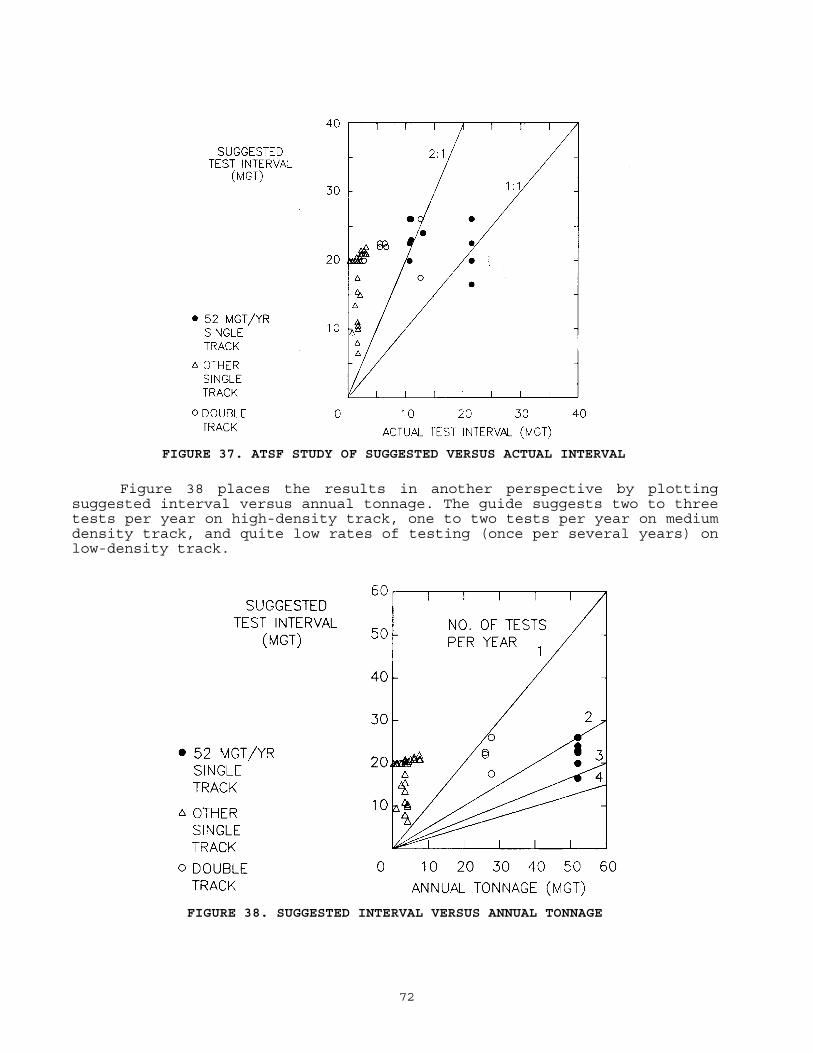
FIGURE 37. ATSF STUDY OF SUGGESTED VERSUS ACTUAL INTERVAL

Figure 38 places the results in another perspective by plotting suggested interval versus annual tonnage. The guide suggests two to three tests per year on high-density track, one to two tests per year on medium density track, and quite low rates of testing (once per several years) on low-density track.

FIGURE 38. SUGGESTED INTERVAL VERSUS ANNUAL TONNAGE

72

Figure 39 is a similar plot of actual test interval versus annual tonnage. The railroad's practice of two to four tests per year is more conservative than the guide (compare Figures 38 and 39). Note also that even the low-density segments are tested two to four times per year, i.e., the schedule is driven by the requirements for testing the high-density track.

FIGURE 39. ACTUAL INTERVAL VERSIS ANNUAL TONNAGE

The SP and UP studies were confined to high-density single track and may be compared with the corresponding part of the ATSF study (Table 10). Figure 40 illustrates the results. In general, the suggested test interval is either equal to current practice or about twice as long. In a few cases, however, the guide did suggest a slightly shorter interval.

The open triangle symbol near the bottom of the graph is a special case. This data point and the solid triangle immediately above represent the same track segment. This segment originally contained bolted-joint rail but was converted, to CWR (without rail renewal) at about the period from which the input data was obtained. The shorter of the two suggested intervals resulted from the inclusion of a large number of bolt hole breaks in the service defect count, while the longer interval was obtained by omitting these defects. This example illustrates a way in which the guide can be used to present a tradeoff between trackwork and frequency of rail testing.

The UP data points in Figure 40 are averages based on annualized calculations similar to those in the ATSF and UP studies. In its own study, however, the UP did evaluate the guide on a per-test basis. Some of the UP segments exhibited seasonal effects, and on these the railroad found that the suggested intervals tended to lag behind current practice

73

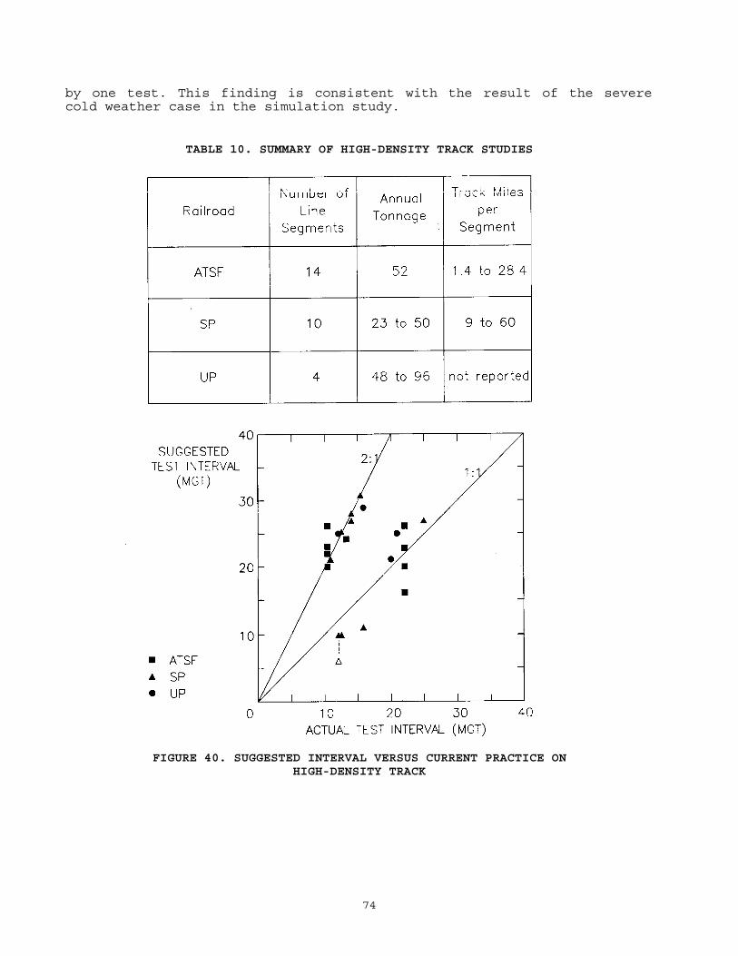
by one test. This finding is consistent with the result of the severe cold weather case in the simulation study.

FIGURE 40. SUGGESTED INTERVAL VERSUS CURRENT PRACTICE ON HIGH-DENSITY TRACK

TABLE 10. SUMMARY OF HIGH-DENSITY TRACK STUDIES

74

5. DISCUSSION

The proposed guide for rail test scheduling provides a workable basis for a rail integrity performance specification. The chart format (Figure 22) is reasonably convenient for practical application, although the explanation of its use must be clarified. The service defect rate performance target is consistent with the national average for modern track and current rail testing technology. When compared with current schedules f or medium to high-density track, the guide generally suggests the same or longer intervals between tests. This is also consistent with the national average, since the railroads operating on such lines have the resources to test more frequently and do so in accordance with their own policies.

The results of the study suggest that some benefits can be gained by adopting the flexible scheduling strategy. Under the present standards, it appears that annual testing of low- and medium-density lines is more frequent than necessary based on the formation, growth, and detectability characteristics of typical rail defects. The guide would generally allow lower test frequencies in those cases, saving equipment usage and labor. Conversely, the guide would likely require somewhat more frequent testing on high-density lines carrying more than 70 MGT per year, reducing the savings to some extent.

The study also shows that the guide is slowly self-adaptive, i.e., it tends to react properly to long-term changes in the environment. The self-adaptation has the potential benefit of automatically relaxing the test frequency requirement in response to improvements in rail manufacturing quality and/or test equipment performance.

However, the proposed guide falls short of being a complete specification suitable for managing the scheduling of rail tests on revenue track. Three items remain to be addressed before a specification can be drafted: (1) how to handle double track territory; (2) how to define a line segment; and (3) how to deal with seasonal effects. Consideration of these three items also raises a common issue, viz: can a specification be based on the guide without imposing an unacceptable paperwork burden on the railroads while still providing clear criteria for compliance? The following subsections offer some answers.

5.1 Treatment of Double Track

On the division studied by the ATSF, the mainline consisted of alternating segments of single and double track, with one of the two tracks being included from each double-track segment. The annual tonnages reported f or the double-track segments were generally half the tonnages reported for the adjacent single-track segments, yet both groups were tested the same number of times per year. These facts suggest a roughly

75

equal division of traffic on the double-track segments and a practice of testing the whole line at a frequency dictated by rail quality goals established for the more heavily utilized single track.

On other lines, however, different operating practices may divide traffic unequally. The division of traffic on double-track territory is not a simple matter, and it is unlikely that many railroads would keep detailed statistics on annual tonnage for every stretch of double track in their systems. Therefore, an accounting procedure based on total tonnage should be sought. The patterns of traffic on different kinds of double track (Figure 41) suggest several possibilities.

Single track with occasional passing sidings can be treated simply as single track. The function of the sidings is to hold trains for opposing traffic, i.e., operations on the sidings are generally at low speed and do not accumulate much tonnage. Thus, most passing sidings should not fall within the scope of a rail integrity specification. Total tonnage on the line, defects on the main track, and route miles are then the appropriate measures of usage, performance, and track length. (Sidings equipped with high-speed turnouts are exceptions and should be included.)

Alternating single/double track presents the most difficult accounting problem because of the effects on tonnage ambiguity on measurements of usage and performance. The following are possible procedures, based on total tonnage, each with advantages and disadvantages:

(1) Restrict the counting of defects and miles to the single-track segments when preparing inputs for the performance chart, but apply the suggested test interval to all segments. This is similar to some current practices (e.g., ATSF). However, a track chart breakdown must. Be used to sort countable from noncountable defects and define the segment length for defect rate calculations. Also, double-track segments will tend to be overtested.

(2) Use route miles and count all defects (i.e., from both tracks in the double-track segments). This avoids the need for a track-chart breakdown. However, the accounting effectively doubles the defect rates on double-track segments with equal traffic division. The doubled rates may be either below or above the rates on adjacent single track. If below, the single-track segments may be somewhat undertested. If above, the whole line will tend to be overtested. Based on the Weibull life distribution with α = 3, the transition from below to above would occur at about 340 MGT on heavy haul lines (β = 1,000 MGT) or 680 MGT on average mixed freight lines (β = 2,000 MGT).

76

(3) Use route miles but, in the double-track segments, restrict counting to the track with the greater number of defects. This avoids the problems caused by doubled defect rates, but requires a track-chart breakdown. Also, double-track segments with equally divided traffic will tend to be overtested.

Interlocked double track with either balanced or predominant one-way traffic can be treated like two single, tracks f or the purpose of applying the guide. No ambiguity is involved if records of annual tonnage are available for each track. If only total tonnage is available, an equal division of traffic can be assumed. The assumption will lead initially to undertesting of the more heavily used track and vice versa. In the long run, however, the differences between assumed and actual tonnage will appear to the guide as a deviation. The self-adaptation feature will then work to adjust to more frequent testing on the more heavily used track and less frequent testing on the other track.

FIGURE 41. TRACK AND TRAFFIC PATTERNS

5.2 Definition of Line Segment

Track segments as short as 0.1 mile were included in the ATSF evaluation of the performance chart. This level of detail was useful for study purposes, and the results showed some consistency in the test interval estimates obtained for contiguous track segments. However, it would be impractical to consider the routine use of such a detailed

77

breakdown for actual test scheduling. Even on those railroads that have computerized track databases, the track engineers could not devise a practical test schedule directly from the large number of individual intervals. A practical schedule might be based on some average of the individual numbers, but then it is equally reasonable and less burdensome to set a lower limit for the length of a line segment and let the track itself do the averaging.

On the other hand, it is not advisable to average over too much track, or important local effects on rail integrity may not be recognized. Therefore, an upper limit on the length of a line segment must also be set.

Reasonable numbers for these limits can be estimated from current practices. For example, Figure 42 illustrates the distribution of lengths of the segments defined in the ATSF and SP studies. Over half the segments (mainly from the low to medium density ATSF tracks) were less than 20 miles long, while very few segments were more than 50 miles long. The lengths of 20 and 50 miles thus appear to be reasonable practical limits for the definition of a line segment in a rail integrity specification.

FIGURE 42. DISTRIBUTION OF TRACK SEGMENT LENGTHS IN THE STUDY

78

5.3 Treatment of Seasonal Effects

When track is subjected to seasonal effects that require more frequent rail testing in cold weather, the guide tends to get out of synchronization and recommend just the opposite. This was shown in the simulation study and was also found in one railroad's evaluation.

The obvious solution to this problem is to leave the seasonal scheduling details to the discretion of the track engineer and to apply the guide only on an annual basis. The annual basis is also consistent with current record-keeping practices. A procedure for, doing so was worked out and applied during the railroad evaluation studies.

The procedure works well for high-density lines but is difficult to apply to other situations. Medium-density lines may be tested at frequencies between one and two times per year. Some low-density lines may not require testing more often than once every two or three years. In such circumstances the number of tests per year can become a wildly fluctuating artifact of the annual accounting procedure.

The artifact can be removed and accuracy can be restored to a large extent, while the convenience of annual accounting is retained, by allowing the guide to be applied on a multiyear basis in some cases. The concept of such an approach is to identify a group of tests which can be treated, for practical purposes, as a repeating cycle and which spans a calendar interval close to a whole multiple of years. The individual intervals which make up the cycle may vary at the discretion of the track engineer, just as in the case of seasonal adjustments discussed earlier. However, the guide would be applied based on the average statistics determined from totals of tonnage, tests, and defect counts for the years covered. This is similar to the annualized procedure discussed earlier (see Section 3.3).

Figure 43 presents several hypothetical examples to illustrate how different test cycles can be matched to annual records. Part (a) illustrates what has already been done in the railroad studies of frequently tested lines. The bars represent time, divided into calendar years, and each triangle symbol represents a rail test. In this case, the track engineer has chosen to concentrate his tests in cold weather. The repeating cycle is close to twelve months long but does not coincide with a calendar year. To apply the guide, the track engineer uses the annual tonnage and defect counts for the current calendar year (represented by the hatched bar) together with the tests at the end of each interval in the cycle (the four solid triangles). Thus, the average existing test interval and defect rates are respectively one fourth of their annual values.

79

Part (b) illustrates a case representing a medium-density line which is being tested at intervals of 8 to 10 months, resulting in an alternation between one and two tests per year. Straight annual accounting would either penalize the railroad or allow too much relaxation of the test schedule, depending on the accounting year. However, a three-test cycle somewhat longer than two years can be identified, and the guide can be applied based on the sum of tonnage and defect data for two years.

Part (c) illustrates three cases representing low-density lines. In the first case, the test interval is 12 months, and the annual procedure can be used. In the second case, the interval is about 16 months, and three solutions are possible. Annual accounting may be used as shown, the annual accounting might be based on the preceding year's data, or the cycle might be extended and two years of data used. In the third case, the test interval is close to 24 months, and two years of data would be used.

FIGURE 43. COMPARISON OF ACTUAL AND ACCOUNTING CYCLES

80

5.4 Compliance Criteria

The foregoing discussion suggests that application of the scheduling guide can be thought of as a process of laying a ruler down to make a measurement. The "ruler" is defined by its lengths in space (20 to 50 track miles) and time (one or more calendar years). Laying down the ruler selects the data to be used, and the measurement is an assessment of the test schedule based on averages. The procedures thus defined work conveniently with annual records and are immune to seasonal lag. The determination of compliance reduces to the question of whether the average interval between tests meets the minimum requirement derived from the performance chart.

Further refinements of language are required to define unambiguous terms of application. These will no doubt involve some approximations (e.g., test cycles not coincident with calendar years) and may require additional adjustments (e.g., a tonnage and defect rate multiplier for cycle lengths different from a whole-year multiple). The terms of application and adjustment factors, together with the performance chart and its procedural rules, could serve as a rail integrity specification.

How might such a specification be employed in practice? In particular, could it be employed without creating a paperwork burden? One way to do so would be to use the specification as a tool for management by exception and spot checking. The railroads would not be required to use the specification to schedule tests but would (via its publication) be able to anticipate its consequences. Under the management-by-exception concept, a railroad track engineer might work through the specification to check the test schedule on some line segments where, in the engineer's judgment, the existing schedule might require modification to meet minimum requirements. Even these calculations would not be required to be kept as official records. Official paperwork would be limited to spot checks carried out by FRA track inspectors. These checks would be performed by means of an audit of the railroad's records for one or more line segments, as defined in accordance with the terms of application.

81

6. CONCLUSIONS

Rail integrity can be controlled by scheduling tests for defects at a frequency consistent with rail usage and defect detection efficiency. These factors can vary widely with respect to track location, season, and rail age. However, annual tonnage and defect rates are good indicators for guidance of the test schedule.

A performance chart has been developed for the purpose of guiding rail test schedules based on tonnage and defect rates. The chart reacts to rail age, as indicated by the combined rates of service and detected defects. The chart also includes a self -adaptive feature which adjusts the test schedule to compensate for changing long-term trends (e.g., changes in rail quality or defect detection efficiency) indicated by changes in service defect rates.

The performance target is 0.1 service defect per track mile between tests. This target is consistent with the current performance average for U.S. railroads. In comparison with current standards and practices, the test intervals derived from the chart tend to be longer for low-density track (annual tonnage less than 20 MGT) and shorter for some high-density track (annual tonnage more than 70 MGT).

The chart format was originally designed for use on a per-test/per-track basis. However, it can also be used to establish average test intervals for annual or multi-year test cycles and/or for double track. Time averaging leads to better results by smoothing out seasonal effects which would otherwise place individual intervals out of phase with respect to the real requirements of the test cycle. Applying the chart to double track can introduce errors, but the self-adaptive feature of the guide can compensate for some of these errors.

In order to construct a rail integrity specification, the performance chart must be supplemented by rules for its use, for definition of a line segment (the length of track for one application of the guide procedures), and for selection of an annual or multi-year accounting base. Suggestions have been made for these rules, but further development of precise language for them is still required.

The rail integrity specification need not require any paperwork by the railroads beyond their current practices of keeping records of annual tonnage and defect reports. Railroads may, at their own option, work through the specification procedures in order to anticipate the status of their trackage and identify requirements for test schedule modification. Compliance can be effected by means of annual records audits conducted by FRA track inspectors in accordance with the specification procedures. Both anticipation and compliance checks can be focused on isolated line segments where the potential for exceptions is perceived.

82

REFERENCES

Abbott, R.A. and Zarembski, A.M., 1978: "On the Prediction of Fatigue Life of Rails," American Railway Engineering Association Bulletin 661, vol. 79, 191-202.

Ahlbeck, D.R. et al., 1980: "Measurements of Wheel/Rail Loads in Class 5 Track," Battelle Columbus Laboratories, Columbus, OH, FRA/ORD-80/19.

Besuner, P.M., Stone, D.H., DeHerrera, M.A., and Schoeneberg, K.W., 1978: "Statistical Analysis of Rail Defect Data (Rail Analysis Volume 3)," AAR Chicago Technical Center, Chicago, IL, report no. R-302.

Breiman, L., 1973: Statistics: With a View Toward Applications, Houghton Mifflin Company, Boston.

Broek, D., 1988: The Practical Application of Fracture Mechanics, Kluwer Academic Publishers, Norwell, MA.

Cannon, D.F., 1989: private communication, Research Department, British Railways Board, Derby, UK.

Davis, D.D., 1987: "Rail Performance Model - User's Manual," AAR Chicago Technical Center, Chicago, IL, report no. R-654.

Davis, D.D., Joerms, M.J., Orringer, O. and Steele, R.K., 1987: "The Economic Consequences of Rail Integrity, "AAR Chicago Technical Center, Chicago, IL, report No. R-656.

Fowler, G.J., 1976: "Fatigue Crack Initiation and Propagation in Pearlitic Rail Steels," PhD thesis, University of California at Los Angeles.

Griffith, A.A., 1920: Transactions of the Royal Society (A) vol. 221, p. 103.

Groom, J.J., 1983: "Determination of Residual Stresses in Rails," Battelle Columbus Laboratories, Columbus, OH, DOT/FRA/ORD-83/05.

Hahn, G.J. and Shapiro, S.S., 1967: Statistical Models in Engineering, Wiley, New York.

Hertz, H., 1895:, "Uber die Beruhrung Fester Elastischer Korper," Gesammelte Werke von Heinrich Hertz 1, Leipzig, 155-173.

Hetenyi, M., 1983: Beams on Elastic Foundation, University of Michigan Press, Ann Arbor, MI.

Irwin, G.R., 1964: "Structural Aspects of Brittle Fracture," Applied Materials Research vol. 3, 65-81.

Jensen, R.S., 1950: "Fatigue Tests of Rail Webs," American Railway Engineering Association Bulletin, vol. 51, 640-647.

R-1

Jeong, D. Y. et al., 1987: "Beam Theory Predictions of Shell Nucleation Life," Contact Mechanics and Wear of Rail/Wheel Systems II (G.M.L. Gladwell, H. Ghonem, and J. Kalousek,, ed.), University of Waterloo Press, Waterloo, Ontario, Canada, supplement.

Journet, B.G. and Pelloux, R. M., 1987: "A Direct Method for Laboratory Spectrum Crack Growth Testing," Theoretical and Applied Fracture Mechanics 7, 19-22.

Journet, B.G. and Pelloux, R.M., 1988: "A Methodology for Studying Fatigue Crack Propagation Under Spectrum Loading: Application to Rail Steels," Theoretical and Applied Fracture Mechanics 8, 117-123.

Lindh, D.V., Taylor, R.Q., and Rose, D.M., 1977: "Sleeve Expansion of Bolt Holes in Railroad Rail," Boeing Commercial Airplane Company, Seattle, WA, final report on contract DOT-TSC-1048 (vols. I and ii).

Lindh, D.V., Taylor, R.Q., and Rose, D.M., 1979: "Sleeve Expansion of Bolt Holes in Railroad Rail," Boeing Commercial Airplane Company, Seattle, WA, final report on contract DOT-TSC-1048 (vol. III).

Mack, G.A. et al., 1984: "Analysis of Rail Defect Data from the Burlington Northern Railroad and the Atchison, Topeka, and Santa Fe Railroad," Battelle Columbus Laboratories, Columbus, OH, DOT/FRA/ORD-84/06.

Mayville, R.A. and Hilton, P.D., 1984: "Fracture Mechanics Analysis of a Rail-End Bolt Hole Crack," Theoretical and Applied Fracture Mechanics 1, 51-60.

Mayville, R.A., Hilton, P.D., and Peirce, D.C., in press: "Investigation of Rail Bolt Hole Cracks," Arthur D. Little, Inc., Cambridge, MA, final report, contract no. DTRS57-83-C-00078.

Miner, M.A., 1945: "Cumulative Damage in Fatigue," J Applied Mechanics 12, A159-Al64.

Orringer, O. and Ceccon, H.L., 1980: "Detection of Rail Defects and Prevention of Rail Fracture," Proc, 31st MFPG Symposium on Failure Prevention in Ground Transportation Systems, National Bureau of Standards, Gaithersburg, MD.

Orringer, O. and Bush, M.W., 1983: "Applying Modern Fracture Mechanics to Improve the Control of Rail Defects in Track," American Railway Engineering Association Bulletin 689, vol. 84, 19-53.

Orringer, O., Morris, J.M., and Steele, R.K., 1984: "Applied Research on Rail Fatigue and Fracture in the United States," Theoretical and Applied Fracture Mechanics l, 23-49.

R-2

Orringer, O., Morris, J.M., and Jeong, D.Y., 1986: "Detail Fracture Growth in Rails: Test Results," Theoretical and Applied Fracture Mechanics 5, 63-95.

Orringer, O. , 1988: "Rail Testing: Strategies for Safe and Economical Rail Quality Assurance," Rail: Replacement Strategies and Maintenance Management, National Research Council, Transportation Research Board, Transportation Research Record 1174, 28-42.

Orringer, O. and Steele, R.K., 1988: "Structural Integrity of Rail in Railroad Track in the United States," Fracture Mechanics: Nineteenth Symposium, ASTM STP 969 (T.A. Cruse, ed.), American Society for Testing and Materials, Philadelphia, PA, 260-278.

Orringer, O. et al., 1988: "Crack Propagation Life of Detail Fractures in Rails," DOT Transportation Systems Center, Cambridge, MA, DOT/FRA/ORD-88/13.

Palmgren, A., 1924: "Die Lebensdauer von Kugellagern," Z.V.D.I. 68, 339-341.

Perlman, A.B. et al., 1982: "Rail Flaw Growth Investigations," American Railway Engineering Association Bulletin 688, vol. 83, 536-550.

Rice, R.C. and Broek, D., 1982: "Fatigue Crack Initiation Properties of Rail Steel," Battelle Columbus Laboratories, Columbus, OH, DOT/FRA/ORD-82/05.

Sih, G.C., 1979: "Mechanics of Crack Growth: Geometrical Size in Fracture," Fracture Mechanics in Engineering Application (G.C. Sih and S.R. Valluri, ed.), Sijthoff and Noordhoff, Leyden, Netherlands, 3-29.

Sih, G. C. and Tzou, D. Y., 1984: "Three-Dimensiona1 Transverse Fatigue Crack Growth in Rail Head," Theoretical and Applied Fracture Mechanics 1, 103-115.

Sih, G.C. and Tzou, D.Y., 1985: "Rail-End Bolt Hole Fatigue Crack in Three Dimensions," Theoretical and Applied Fracture Mechanics 1, 97-112.

Sines, G. and Waisman, J. L. (ed.), 1959: Metal Fatigue, McGraw-Hill, New York, 145-169.

Sperry Rail Service, Danbury, CT, 1964: Rail Defect Manual.

Steele, R.K. and Reiff, R.P., 1982: "Rail: Its Behavior in Relationship to Total System Wear," Proc. Second International Heavy Haul Railway Conference, Colorado Springs, CO.

R-3

Stone, D.H. and Knupp, G.G. (ed.), 1978: Rail Steels - Developments, Processing, and Use, ASTM STP 644, American Society for Testing and Materials, Philadelphia, PA.

Talbot, A.N. et al., 1930: "Fifth Progress Report of the Special Committee on Stresses in Track," Proc. American Railway Engineering Association 31, 69-336.

Timoshenko, S. and Langer, B. F., 1932: "Stresses in Railroad Track, ASME Transactions 54, 277-293.

Thomas, J.W., 1985: "1983-1984 Statistical Analysis," Sperry Railer 52, 1-5.

Weibull, W., 1951: "A Statistical Distribution Function of Wide Applicability," J Applied Mechanics 18, 293-297.

Weibull, W., 1961: Fatigue Testing and Analysis of Results, Pergamon Press, New York.

Wohler, A.: 1858 vol. 8, 641-652; 1860 vol. 10, 583-616; 1866 vol. 16, 67-84; 1870 vol. 20, 73-106: Zeitschrift fur Bauwesen.

Zarembski, A.M., 1979: "Effect of Rail Section and Traffic on Rail Fatigue Life," American Railway Engineering Association Bulletin 673, vol. 80, 514-527.

R-4