Control of ion loss from Mars during solar minimum S. H. BRECHT AND S. A. LEDVINA: CONTROL OF ION...

Earth Planets Space, 64, 165–178, 2012

Control of ion loss from Mars during solar minimum

Stephen H. Brecht1 and Stephen A. Ledvina2

1Bay Area Research Corp., P.O. Box 366, Orinda, CA 94563, USA2Space Sciences Laboratory, UC Berkeley, 7 Gauss Way, Berkeley, CA, USA

(Received February 10, 2011; Revised May 14, 2011; Accepted May 30, 2011; Online published March 8, 2012)

A hybrid particle code has been used to examine the interaction of the solar wind with Mars during solarminimum. The results were surprising as they produced ion loss rates from Mars far in excess of what is estimatedfrom MEX. The results are analyzed and found to be consistent with the competition between photochemicalrates and advection of the ionosphere. The simulations showed significant erosion of the ionosphere at altitudesbetween 200 km and 250 km altitudes. Addition of the crustal magnetic fields reduced the erosion and reducedthe ion loss rates to a level consistent with the data.Key words: Mars, ionospheric loss, crustal magnetic fields, simulation, solar wind interactions.

1. IntroductionThe loss of Mars’ atmosphere has been a topic of con-

siderable research and conjecture. A variety of researchgroups are attempting to accurately estimate the loss rate us-ing numerical techniques. Many others are examining datacoming from the latest spacecraft to Mars, Mars Express(MEX). In this paper the results of our latest and improvedhybrid simulations will be presented. The focus of this pa-per is the change of estimated loss rates as a function of avariety of parameters as well as changes in the numericalmodels/resolution being applied to the simulations of Mars.

Mars is one of the unique bodies on the solar system. Itis small planet with a relatively mild temperature (as com-pared to the outer planets or Venus and Mercury), and it haswater on its surface (Di Achille and Hynek, 2010). Becauseit has some water now and apparently had much more waterin earlier epochs, it is a prime location to hunt for life wemight recognize. Mars also offers an opportunity to studyand understand many aspects of planetary atmospheres. Itssmall size means that the bow shock of Mars does not ef-fectively thermalize the solar wind plasma in the subsolarregion. There is limited space between the shock and theionosphere relative to the collisional mean free path and theion gyroradii of the incoming protons. In addition there is alimited amount of time for the electromagnetic thermaliza-tion process to occur (Brecht and Ferrante, 1991). Finally,its small size means that Mars has an extensive exosphere,relatively larger than any other planet (Kim et al., 1998).

The solar wind interaction with a planet unprotected byan extensive intrinsic field has been the subject of consider-able study. The research has come in two forms; missionsto the planets Mars and Venus, and numerical simulations.The number of papers from the Pioneer Venus Orbiter num-

Copyright c© The Society of Geomagnetism and Earth, Planetary and Space Sci-ences (SGEPSS); The Seismological Society of Japan; The Volcanological Societyof Japan; The Geodetic Society of Japan; The Japanese Society for Planetary Sci-ences; TERRAPUB.

doi:10.5047/eps.2011.05.037

bers in the thousands. The number of papers from missionsto Mars is rapidly approaching a similar magnitude if notlarger. One of the features seen in the data from these mis-sions to Mars and Venus is that the solar wind interacts di-rectly with the atmosphere/ionosphere/exosphere of theseplanets. This interaction is found to result in the loss ofions from these two planets. The current understanding ofthe solar wind interaction with Mars has been reviewed byMazelle et al. (2004) and Nagy et al. (2004).

Major research questions revolve around the issues of theamount of water on Mars in the past and where it may havegone. There are a variety of theories on this topic. Oneof the more interesting and complete papers concerningthis topic is by Lammer et al. (2003). In this paper theauthors discuss the various mechanisms for water loss andthe issue of water being tied up in the soil. The pick up ofoxygen ions via the solar wind interaction with the Martianionosphere/exosphere is proposed to be one of the majorloss mechanisms (cf., Lammer and Bauer, 1991; Lundin etal., 1991, 2006; Lammer et al., 1996). Fox (1997) producedan estimate of what it would take to achieve the 2:1 ratio ofhydrogen to oxygen for water loss. In her estimate the rateneeded to be roughly 1 × 1026 oxygen atoms per secondor 1.2 × 108 cm−2 s−1. It is worth noting that a loss rateof 1026 oxygen ions per second would remove a meter ofwater from the entire surface of Mars in 1.72 Gy. Data fromPhobos-2, which orbited Mars during the solar maximumperiod, indicates a loss rate of 3 × 1025 ions s−1 (Lundin etal., 1989, 1990).

Over the past two decades a series of spacecraft havebeen sent to Mars. Phobos-2 was the first to measure lossrates for heavy ions (O+ and O2

+ being the major con-stituents). These measurements occurred during solar max-imum and found loss rates above 1025 particles per second(Lundin et al., 1989, 1990; Verigin et al., 1991). Laterthe Mars Global Surveyor arrived and made a major dis-covery: the presence of strong crustal magnetic fields onMars (Acuna et al., 1998). Finally, the Mars Express mis-

165

166 S. H. BRECHT AND S. A. LEDVINA: CONTROL OF ION LOSS FROM MARS DURING SOLAR MINIMUM

sion arrived during solar minimum and began making mea-surements of plasma environment around Mars and foundloss rates for O+ ranging from 1023 particles/s (Barabash etal., 2007) to >1024 particles/s (Lundin et al., 2008). Typi-cally the estimates from the spacecraft found O+ loss ratesslightly higher than the O2

+ loss rates. Lundin et al. (2009)suggest that the cold ion loss rates do not support the 2:1ratio of H+ to O+ needed to explain water loss however thisargument does not include the traditional thermal loss ofneutral H from the atmosphere. Estimates by Fox (2009)predict that the O2

+ loss rates should dominate the O+ lossrates. As will be discussed later, accurate loss rate estimatesfrom spacecraft data are difficult to make because of thecomplex geometry of the loss regions on Mars coupled withthe fact that the removed O2

+ is not found in the same lo-cations as the O+. While there is overlap in the respectiveion loss regions, O2

+ ions are found upstream of the planetand the bow shock as well as being more structured in the“north pole” region. In this paper we define the term “northpole” as the direction of the convection electric field per-pendicular to the solar wind flow and the plane containingthe IMF often in the +z direction in Mars-Sun coordinates.

The research to be reported in this paper will focus on thesolar minimum situation. Specifically, the paper will exam-ine the various aspects of the Martian interaction with thesolar wind during the minimum period of solar activity andprovide some insight into how various aspects of the inter-action occurs. The main measure of merit will be the totaloxygen ion loss rates. The paper will also examine the ef-fects of improving the chemistry models and the importanceof “getting the chemistry right”. The simulations are part ofearlier research and our participation the code comparisonmeetings convened in 2009 at the International Space Sci-ence Institute, ISSI, in Bern Switzerland (Brain et al., 2010;Nilsson et al., 2010). The “ISSI” meeting led to a challengeto perform a series of simulations with very detailed inputconditions for comparison between the various simulationgroups. For ease of comparison all of the test simulationswere performed without the presence of the crustal mag-netic field.

In the next section a discussion of the numerical modelused and how it compares to other models will be presented.A discussion of the solar minimum results will follow. Thelast two sections will present a discussion of the results andthen conclusions.

2. Numerical ApproachIt has been found by researchers examining data, as well

as, those performing simulations that the interaction of thesolar wind with Mars leads to a very asymmetric interactionregion and rapid variations in measured quantities. Thesecharacteristics mean that by the very nature of spacecraftdata collection there are large spatial and temporal holes inthe planetary coverage. Nevertheless, the data from space-craft such as Phobos-2, Mars Global Surveyor, and MarsExpress, (MEX), provide a wealth of information. How-ever, the only way to fully understand the nonlinear andcomplex interactions suspected to occur within the iono-sphere and atmosphere of Mars is via simulation coupledto comparisons to spacecraft data.

To estimate the global loss of oxygen from Mars scien-tists have employed two distinct numerical approaches tomake these estimates. One is the MHD formalism (cf., Liuet al., 2001; Ma et al., 2002, 2004; Ma and Nagy, 2007;Harnett and Winglee, 2006) and the second is the kineticformalism, specifically the hybrid particle code (cf., Brecht,1990; Brecht and Ferrante, 1991; Kallio and Janhunen,2002; Boßwetter et al., 2004; Modolo et al., 2005; Chanteuret al., 2009). In addition to these two fundamental ap-proaches an ion tracking or Monte Carlo approach us-ing MHD electromagnetic fields has also been tried (cf.,Cravens et al., 2002; Fang et al., 2010 a, b). The ion track-ing approach is an attempt to capture some of the kinetic be-havior not found in the MHD code but has the disadvantagethat the particle motion and fields are not self-consistent un-less only the high energy plasma and not the bulk plasma isconsidered. A detailed discussion of the equations and as-sumptions contained within these approaches can be foundin Ledvina et al. (2008).

The preferable numerical tool is a well resolved kineticparticle code where at least the ions are treated kinetically,such a code is a hybrid particle code. The hybrid modeltreats all ion species (the model can carry as many as onewishes) as kinetic particles. The ions are advanced in ve-locity with a simple Lorentz force equation. The electronsare treated as a massless neutralizing fluid. The electro-magnetic fields are calculated self-consistently with the ionmotion. Electromagnetic waves up to and including a por-tion of the whistler wave spectrum are carried in the code.Shock formation is included in the physics of this code andthus needs no assumptions or numerical techniques to cap-ture the shock. The basic equations of the hybrid modelare well known and need not be repeated here. See Harned(1982), Brecht and Thomas (1988), and Brecht and Ledvina(2006, 2010) for a more complete discussion. The researchreported in this paper employed hybrid particle simulationsusing the HALFSHEL code. The HALFSHEL code hasbeen used in simulations of unmagnetized bodies for manyyears (cf., Brecht, 1990, 1997a, b; Brecht and Ferrante,1991; Brecht et al., 1993, 2000; Ledvina et al., 2004;Brecht and Ledvina, 2006, 2010).

Mars is difficult to simulate because there are three (3)parts to the simulation problem.

• The electromagnetic environment and kinetic phenom-ena such as: ion gyromotion and subsequent non-isotropic pressure tensors

• The ionospheric chemistry• Collisional phenomena within the lower portion of the

ionosphere with the neutral atmosphere.

One must accurately simulate electromagnetic environment(solar wind plasma, solar wind IMF, electromagnetic wavesand the crustal fields of Mars) and the plasma behaviorwhich can have gyro-rotational behavior on a scale largerthan the Mars. Because the solar wind interacts directlywith the atmosphere/ionosphere, one must accurately cre-ate/simulate the atmosphere/ionosphere and this requires achemistry package that can react to the rather rapid loss ofthe ions into the solar wind. A constant production ratehas been found to be inadequate. Worse there is a nominal

S. H. BRECHT AND S. A. LEDVINA: CONTROL OF ION LOSS FROM MARS DURING SOLAR MINIMUM 167

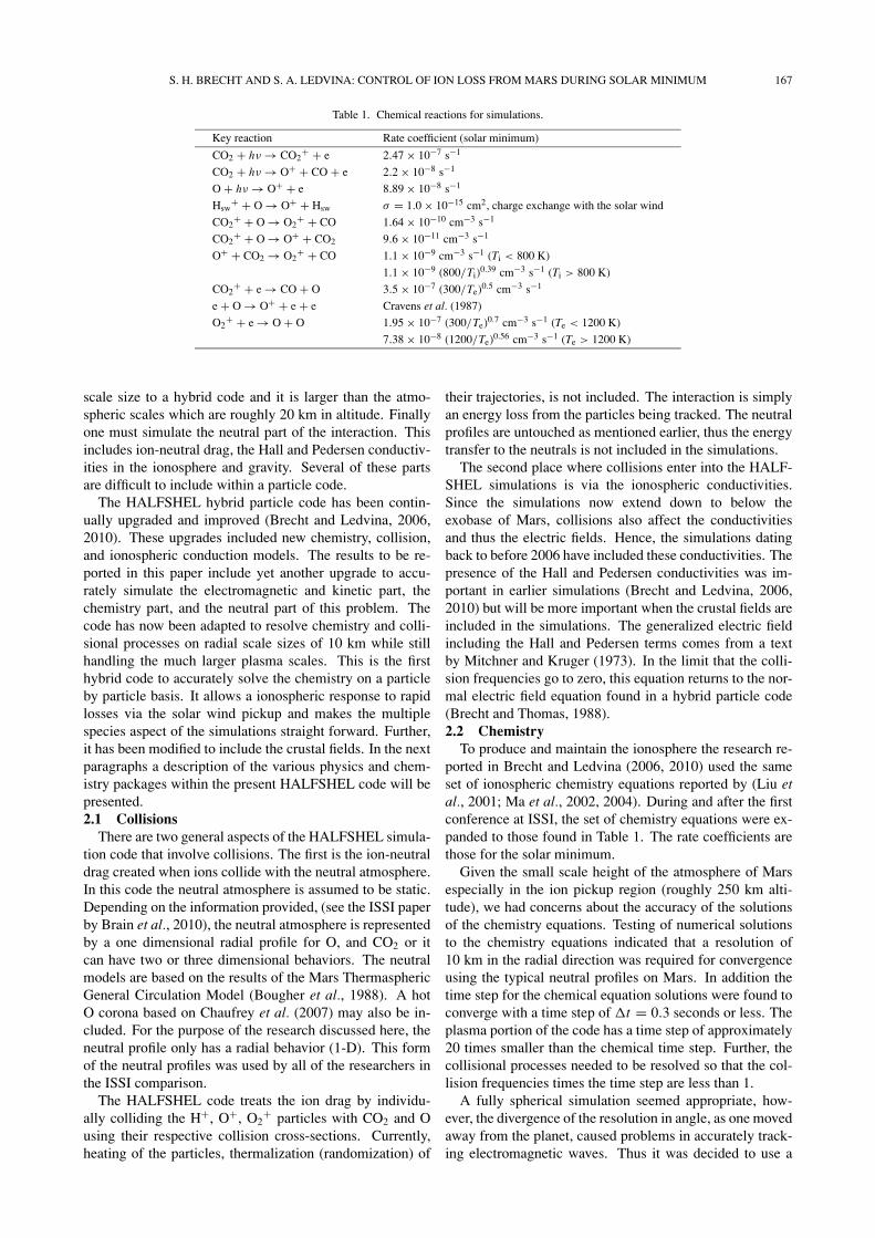
Table 1. Chemical reactions for simulations.

Key reaction Rate coefficient (solar minimum)

CO2 + hν → CO2+ + e 2.47 × 10−7 s−1

CO2 + hν → O+ + CO + e 2.2 × 10−8 s−1

O + hν → O+ + e 8.89 × 10−8 s−1

Hsw+ + O → O+ + Hsw σ = 1.0 × 10−15 cm2, charge exchange with the solar wind

CO2+ + O → O2

+ + CO 1.64 × 10−10 cm−3 s−1

CO2+ + O → O+ + CO2 9.6 × 10−11 cm−3 s−1

O+ + CO2 → O2+ + CO 1.1 × 10−9 cm−3 s−1 (Ti < 800 K)

1.1 × 10−9 (800/Ti)0.39 cm−3 s−1 (Ti > 800 K)

CO2+ + e → CO + O 3.5 × 10−7 (300/Te)0.5 cm−3 s−1

e + O → O+ + e + e Cravens et al. (1987)

O2+ + e → O + O 1.95 × 10−7 (300/Te)0.7 cm−3 s−1 (Te < 1200 K)

7.38 × 10−8 (1200/Te)0.56 cm−3 s−1 (Te > 1200 K)

scale size to a hybrid code and it is larger than the atmo-spheric scales which are roughly 20 km in altitude. Finallyone must simulate the neutral part of the interaction. Thisincludes ion-neutral drag, the Hall and Pedersen conductiv-ities in the ionosphere and gravity. Several of these partsare difficult to include within a particle code.

The HALFSHEL hybrid particle code has been contin-ually upgraded and improved (Brecht and Ledvina, 2006,2010). These upgrades included new chemistry, collision,and ionospheric conduction models. The results to be re-ported in this paper include yet another upgrade to accu-rately simulate the electromagnetic and kinetic part, thechemistry part, and the neutral part of this problem. Thecode has now been adapted to resolve chemistry and colli-sional processes on radial scale sizes of 10 km while stillhandling the much larger plasma scales. This is the firsthybrid code to accurately solve the chemistry on a particleby particle basis. It allows a ionospheric response to rapidlosses via the solar wind pickup and makes the multiplespecies aspect of the simulations straight forward. Further,it has been modified to include the crustal fields. In the nextparagraphs a description of the various physics and chem-istry packages within the present HALFSHEL code will bepresented.2.1 Collisions

There are two general aspects of the HALFSHEL simula-tion code that involve collisions. The first is the ion-neutraldrag created when ions collide with the neutral atmosphere.In this code the neutral atmosphere is assumed to be static.Depending on the information provided, (see the ISSI paperby Brain et al., 2010), the neutral atmosphere is representedby a one dimensional radial profile for O, and CO2 or itcan have two or three dimensional behaviors. The neutralmodels are based on the results of the Mars ThermasphericGeneral Circulation Model (Bougher et al., 1988). A hotO corona based on Chaufrey et al. (2007) may also be in-cluded. For the purpose of the research discussed here, theneutral profile only has a radial behavior (1-D). This formof the neutral profiles was used by all of the researchers inthe ISSI comparison.

The HALFSHEL code treats the ion drag by individu-ally colliding the H+, O+, O2

+ particles with CO2 and Ousing their respective collision cross-sections. Currently,heating of the particles, thermalization (randomization) of

their trajectories, is not included. The interaction is simplyan energy loss from the particles being tracked. The neutralprofiles are untouched as mentioned earlier, thus the energytransfer to the neutrals is not included in the simulations.

The second place where collisions enter into the HALF-SHEL simulations is via the ionospheric conductivities.Since the simulations now extend down to below theexobase of Mars, collisions also affect the conductivitiesand thus the electric fields. Hence, the simulations datingback to before 2006 have included these conductivities. Thepresence of the Hall and Pedersen conductivities was im-portant in earlier simulations (Brecht and Ledvina, 2006,2010) but will be more important when the crustal fields areincluded in the simulations. The generalized electric fieldincluding the Hall and Pedersen terms comes from a textby Mitchner and Kruger (1973). In the limit that the colli-sion frequencies go to zero, this equation returns to the nor-mal electric field equation found in a hybrid particle code(Brecht and Thomas, 1988).2.2 Chemistry

To produce and maintain the ionosphere the research re-ported in Brecht and Ledvina (2006, 2010) used the sameset of ionospheric chemistry equations reported by (Liu etal., 2001; Ma et al., 2002, 2004). During and after the firstconference at ISSI, the set of chemistry equations were ex-panded to those found in Table 1. The rate coefficients arethose for the solar minimum.

Given the small scale height of the atmosphere of Marsespecially in the ion pickup region (roughly 250 km alti-tude), we had concerns about the accuracy of the solutionsof the chemistry equations. Testing of numerical solutionsto the chemistry equations indicated that a resolution of10 km in the radial direction was required for convergenceusing the typical neutral profiles on Mars. In addition thetime step for the chemical equation solutions were found toconverge with a time step of �t = 0.3 seconds or less. Theplasma portion of the code has a time step of approximately20 times smaller than the chemical time step. Further, thecollisional processes needed to be resolved so that the col-lision frequencies times the time step are less than 1.

A fully spherical simulation seemed appropriate, how-ever, the divergence of the resolution in angle, as one movedaway from the planet, caused problems in accurately track-ing electromagnetic waves. Thus it was decided to use a


Fig. 1. This is a schematic of the Cartesian grid upon which the electromagnetic fields are solved and the “spherical” grid where the chemistry andcollisions are applied to existing particles and those being created. The “spherical” grid has been expanded so that one can see some of the details.The radius of the “spherical” grid ranges between 150 km and 600 km to 1000 km.

different tactic. The electromagnetic part of the code wouldbe Cartesian thus the resolution did not change no matterwhere waves or electromagnetic structures were formed. Aset of “spherical” grids were added to the simulation to re-solve the neutral density profiles at much higher accuracyfor a better solution of the chemistry equations shown inTable 1 and to calculate a variety of collisional plasma be-haviors. The term “spherical” is used in this paper, butthe grid is not a true spherical grid as it does not havethe same metric as a true spherical grid: Here the metricis r2drdθdϕ. This makes loading particles and weightingthem much easier as each cell at a given radius is the samesize. This approach works because there are no differentialoperators applied using this grid. The solution of the fieldequations is performed on the Cartesian grid with the par-ticles being allocated to either grid as necessary. Figure 1shows a schematic of the new hybrid code. The sphericalgrid has a typical radial resolution of 10 km and about 1.9◦

angular resolution. It generally covers a range from about150 km altitude to between 600 km and 1000 km in altitude.The range changes depending what neutral profile is beingused and the chemical species being produced.

The chemistry is performed on the particles within thespherical grid. New particles are created if the productionrate exceeds the loss rates within each spherical cell. Previ-ously existing particles have their density decreased as re-combination occurs. These spherical grids (there are sev-eral for each ionospheric species) also are used to calculatethe ion-neutral drag and to apply the gravity terms as well.What makes this particularly effective is that particle loca-tions can be easily found on either grid. Therefore, iono-spheric particles that are picked up will naturally transitionout of the region of chemistry and collisions into the regionof pure collisionless electromagnetic interactions. Mean-while, particles still at lower altitudes feel the electromag-

netic fields from the Cartesian grid as well as the collisionalforces.

The inclusion of the spherical grids into HALFSHELwas a complicated and major step in the evolution towardmore accurate simulations of the solar wind interaction withMars’ ionosphere. As mentioned earlier, the chemistry codewas tested externally to make sure that spatial and tempo-ral convergence is achieved. This testing led to new in-sights concerning the simulations and how we were per-forming them. In earlier work, the ionosphere had beenloaded as a profile and replenished at a specific rate in orderto achieve a full ionospheric profile in a certain time. How-ever, it was discovered that we needed to run the simulationsmuch longer. Instead of 20,000 time steps we needed to use50,000 or more. Although the loss rates are collected bya virtual box at 2Rm it still takes between 1,000 to 2,000seconds for the loss rates to reach a steady state. With thecrustal fields in the simulations the time to reach equilib-rium often exceeds 2,000 seconds, ∼100,000 time steps.If the simulations were run until the particles leaving thewhole computational grid reached steady state considerablylonger runs would be necessary. In the work published in2010 Brecht and Ledvina (2010) resolved the chemistry onthe Cartesian grid. Because the code was using cell sizesof 300 km, it was found that the chemistry did not properlyconverge. With the new capability, the chemistry portion ofthe code converged properly. And at this point some sur-prises were found.

Figures 2 and 3 illustrate the issue. These figures showthe net production rates (production-loss) for O+ as a func-tion of altitude and time with no advection present. Note,in the solar minimum case, Fig. 2, the chemistry at 200 kmtakes over 400 seconds to come into photochemical equilib-rium (net flux = 0). At 250 km altitude (generally above theexobase) it requires ∼5,000 seconds while altitudes above


Fig. 2. The net production rates for O+ at various altitudes during solarminimum conditions.

Fig. 3. The net production rates for O+ at various altitudes during solarmaximum conditions.

300 km requires much longer (>50,000 seconds) to con-verge. At solar maximum the time scales drop due to in-creased neutral density at these altitudes and the increase insolar EUV flux. This led to a quandary. How to perform thesimulations? It was clear that if there was any sort of ad-vection of the ionosphere before it was constructed the sim-ulation would never reach appropriate ionospheric densitiesduring the simulation. This would mean a generally lowerprediction for the ion loss from Mars. The solution was tointegrate the chemistry before the advection of plasma andelectromagnetic fields began. The chemistry was integratedout 10,000–20,000 seconds, depending on the specific situ-ation, until the ionosphere reached photochemical equilib-rium at least up to the exobase. The results can be seen ina comparison of our chemistry to the Viking data, Fig. 4.Here one sees good agreement with the data up to a givenaltitude where it appears that the Martian oxygen ions arebeing advected to the location of the Viking landing.

In summary, the chemistry package has been tested nu-merically for temporal and spatial convergence. This infor-mation was then used in the HALFSHEL code to provide anaccurate ionosphere. The chemistry was also tested againstthe Viking data and found to match well, if the chemistry

Fig. 4. Comparison of the chemistry solution with the Viking data. O+ isa little low compared to the data, but may well be due to advection tothe longitude and latitude of the Viking landing. The solid lines are thechemistry model results.

was properly converged. The addition of the “spherical”grids to allow higher resolution chemistry coupled with thenew strategy for starting the simulation has led to some newinsights into the solar wind interaction with Mars.

3. ResultsThere are many questions and uncertainties that a re-

search program addressing Mars could address. Further, thesimulations have now become very complex with enormousamounts of data being produced. To focus this paper it isworth addressing some of the data and our past discoveriesfrom previous Mars simulations.

Our previous simulations of Mars with the hybrid code(Brecht and Ledvina, 2006, 2010) led to a variety of find-ings. The first was that the loss of particles did not mimicMHD code results (cf., Ma et al., 2002, 2004; Ma and Nagy,2007). The convection electric field tends to accelerate ionsin the “north” pole which is defined as the pole for whichthe convection electric field points away from the planet. Inaddition to this it was found that the shock produced a verynon-isotropic pressure tensor (Brecht and Ledvina, 2010).It has also been found that loss rates are sensitive to theneutral profiles used even if the EUV flux is held constant.It has been repeatedly found that the loss rates do vary withthe EUV flux and this variation seems to be consistent withthe data from spacecraft. One sees that the pickup rates donot change linearly with increased EUV frequency (Brechtand Ledvina, 2010).

Another feature found in the simulations and reported inBrecht and Ledvina (2010) is the restricted region of the en-ergetic ionospheric ions, as they escape. The energetic par-ticles come from the “north pole” which is defined as thedirection of the solar wind convection electric field. Theparticles can reach energies of greater than 10 keV. Theenergetic particles coming from the “north pole” are veryconsistent with measurements reported by Prez-de-Tejadaet al. (2009). The loss region in the pole is very narrow inthe dimension perpendicular to the ambient magnetic field.Of interest is the lower energy ∼10 eV O+ seen to be com-


Table 2. Simulation parameters.

Hot O corona IMF (nT) SW density cm−3 Solar wind vel. (km/s) Crustal field

Solar min. No 3 2.7 485 No

Solar min. Yes 3 2.7 485 No

Solar min. Yes 3 2.7 485 Yes

Solar max. Yes 3 2.7 485 No

Table 3. Loss rates in particles/s.

Solar min. with corona Solar max. with corona Solar min. with corona and crustal fields

O+ 4 × 1024 9.3 × 1024 2.5 × 1023

O2+ 1. × 1026 6. × 1025 3. × 1024

ing from the “southern” hemisphere. In fact more parti-cles are being lost from the “southern” hemisphere than the“northern” hemisphere. This is unexpected as the convec-tion electric field is nominally pointed into the planet on the“southern” hemisphere. However, in the “southern” hemi-sphere one finds a large region were there is at least somecomponent of the electric field parallel to the local mag-netic field which is essentially aligned along the flow axis inthe tail region. The existence of the parallel fields explainshow the O+ is escaping in the “southern” hemisphere. Italso explains some of the observations. The presence of theparallel electric fields was reported in Brecht and Ledvina(2010).

The “ISSI Challenge” called for three specific simula-tions to be performed. Neutral profiles were provided forboth solar maximum and solar minimum. The IMF was3 nT with a 56◦ degree Parker spiral. The solar wind den-sity was 2.7 protons/cm3 with a velocity of 485 km/s. TheCartesian cell resolution was 150 km in each direction, soas to allow comparisons with other hybrid simulations. Thechemistry/collision grid had a resolution of 10 km radially,and 1.9◦ in latitude and longitude.

The total ion loss rate is a marker for what is going onwithin Mar’s ionosphere. The loss rate has been examinedfor the ISSI solar minimum test cases; the solar minimumcase without a hot oxygen corona and the solar minimumcase where there is a hot oxygen corona. The ISSI solarmaximum test case with the hot oxygen corona is also re-ported here. An additional simulation was performed forthe solar minimum case with the Martian crustal magneticfields included. The focus of this paper is the change inionospheric loss rate as a function of these four simulations,Table 2.

The results for the solar minimum and solar minimumwith hot oxygen corona were essentially the same. Al-though, it was shown in Brecht and Ledvina (2010) that thecorona made a modification in the shock location due to theslight change in the solar wind Alfven speed, there werefound no significant difference in the global loss rate. Therates found for these cases are summarized in Table 3. Thesolar minimum case calculated a loss rate of 4 × 1024 parti-cles/s for the O+ and 1 × 1026 particles/s for the O2

+. Inter-estingly, the O2

+ loss rate is consistent with the maximumloss rates predicted by Fox (2009). These numbers repre-sent a reduction of the previous O+ loss rate from our Carte-

sian simulations reported in Brecht and Ledvina (2010),8 × 1024 particles/s. and large increase in the O2

+ loss ratewith this species now the largest of the ion loss species. Thisresult was a complete surprise. It had been expected that theincreased resolution of the chemistry would change the an-swers previously reported, but it was not expected that thenumbers would reach this level. It had been noted by Ma etal. (2004) that the ratio of loss species switched when theywent to higher resolution. The present results seem consis-tent with their findings.

It should be noted that these results are not consistentwith the estimates from the data. Nor are they consistentwith many of the other simulation groups. Interestingly, theloss rates for the solar maximum case with the hot oxygencorona were found to be 9.3 × 1024 particles/s for the O+

and 6. × 1025 particles/s for the O2+. The O+ loss rate

is somewhat low as compared to that reported by Lundinet al. (1989, 1990) but the O2

+ loss rate seems consistent.The solar maximum rates are lower than those found forthe solar minimum case and a bit lower than estimates fromthe data, yet the solar minimum is much higher than theestimates.

Finally, it was thought that perhaps the presence of theMartian crustal magnetic fields might help explain the solarminimum inconsistency with data. So the solar minimumsimulation with the hot oxygen corona simulation was runwith crustal magnetic fields included in the simulation. Inthis case, the field model used was by Purucker et al. (2000).The orientation of the crustal magnetic fields is shown inFig. 5. We have plotted the crustal field at an altitude of200 km with the (0, 0) coordinates at the subsolar point.The magnitude of B is plotted at the resolution of the finegrid (1.9◦ or 112 km resolution in the angular dimensions).The plot is smeared out because we are filling each squarewith the interpolated field. Examination of figures 2 and3 in Acuna et al. (1999) reveals that the resolution is veryconsistent with the data from which Purucker and others(cf. Cain et al., 2003) have created the crustal magneticfield models. The fields applied to the particles via theLorentz force are interpolated field from the Cartesian grid(150 km). The features that the particles feel reflects morestructure than is shown in Fig. 5. However, the generallevel of accuracy is reflected in the plot and this accuracy isconsistent with the data as presented by Acuna et al. (1999).

The results of the simulation with the crustal magnetic


Fig. 5. Orientation of the Martian crustal magnetic fields. The magnitude of B is plotted at 200 km altitude in order to be compared to data from Acunaet al. (1999) (figures 2 and 3). The subsolar point is located at (0, 0) on this plot.

field are as follows: 2.5×1023 particles/s for the O+ and 3.×1024 particles/s for the O2

+ . These results are consistentwith the most recent estimates from the MEX spacecraft:1023 O+ particles/s (Barabash et al., 2007) to >1024 O+

particles/s (Lundin et al., 2008). The predicted loss rateshave changed by roughly 20 for O+ and 30 for O2

+ fromthe previously estimated loss rates. The O2

+ loss rate isroughly 10 times higher than the O+ loss rate, consistentwith Fox (2009).

The results can be summarized as follows: the higher res-olution chemistry simulations produce very different resultsthan previously reported. The solar minimum results do notchange with the addition of the hot oxygen corona. The so-lar minimum results are much higher than estimates fromthe data. Further, moving to the solar maximum situationthe loss rates dropped for the O2

+, but increased by a factorof two for the O+. Finally, inclusion of the crustal magneticfields reduced the solar minimum loss rates to a value con-sistent with estimates from the data. The crustal magneticfield affects are always present in the Mars mission dataunlike many of the simulations reported to date. The non-crustal fields simulations are more like Venus albeit with asmaller planet, smaller ionosphere, and weaker EUV flux.In the next section, the results will be discussed in light offurther analysis of the simulations.

4. DiscussionThe results presented seem to be contradictory. The so-

lar minimum results providing much higher loss rates ofmolecular oxygen ions than atomic oxygen ions. The solarminimum molecular oxygen ion loss rates are higher thanfor solar maximum, while the atomic oxygen ion loss rate islower for solar minimum than solar maximum as expected.Finally, the crustal magnetic fields are found to make a verylarge change in both species loss rates for the solar min-imum case. In the next paragraphs further analysis willbe presented to explain what at first seems to be counter-intuitive results that are to some degree inconsistent withthe data.

One place to begin is to examine the ionosphere. For thepurposes of this discussion the altitude of choice is 250 kmwhich is slightly above the exobase of the nominal iono-sphere. Figure 6(a, b) show the density of the O+ and the

O2+ for the no crustal field solar minimum case. The O+

seems to be greatly reduced in the subsolar region where(0, 0) is the subsolar point in latitude and longitude. TheO2

+ is almost completely removed. In short, the electricfields are penetrating very deeply into the ionosphere andreaching altitudes where the O2

+ density is very high. Ex-amination of Fig. 7(a, b) shows the impact of the crustalmagnetic fields. Note the high levels of the O+ in the sub-solar region dropping off to the night side. This is muchcloser to the initial ionospheric load and reflects the ex-pected day-night drop off in density, see Fig. 8(a, b). TheO2

+, Fig. 7(b), shows a more uniform density as if it is be-ing moved around but being contained in the ionosphere.There are significant holes in the density as one goes to-ward the terminator and the night side, but this may due tothe statistical slice being taken: a 10 km slice at an instantin time. Enhancements and holes have been reported bya variety of researchers (cf., Nielsen et al., 2007; Gurnettet al., 2010). Both papers address the MARSIS data setsand found the enhancements were associated with crustalmagnetic field cusps. At this point we cannot address thisobservation other than to point out the structure observed ina snapshot of the simulation. Yet, one can see from Fig. 6(a,b) and Fig. 7(a, b) that the structure in the ionosphere espe-cially on the night side is only seen with the crustal fieldsin the model. This strongly suggests that the crustal fieldare the source of the structure at 250 km and the structuremay be smaller size and more intense at lower altitudes.Since the MARSIS data requires 1.2 s to acquire, summingand averaging the simulation results over that length of timewould be required for accurate comparisons.

Examining the radial velocity for each of these speciesprovides more insight into what is occurring. Figure 9(a, b)show the radial velocity profile for both species. One seesthat there are enhanced radial velocities in the polar regionsespecially the north pole and that the velocity is greatlyenhanced on the night side of the planet. In Fig. 10(a, b)the radial velocity for both species is shown for the crustalmagnetic field situation. One sees very low radial velocitieswith little spatial variation from day to night. This suggeststhat the pick up region is above 250 km when the crustalmagnetic fields are included. This is consistent with themuch lower loss rates and the very significant drop in the


(a)

(b)

Fig. 6. The density of atomic (a) and molecular oxygen (b) ions with the no crustal magnetic fields present. The coordinate (0, 0) is the subsolar pointon these plots.

(a)

(b)

Fig. 7. The density of atomic (a) and molecular oxygen (b) ions with the crustal magnetic fields present. The coordinate (0, 0) is the subsolar point onthese plots.


(a)

(b)

Fig. 8. Contours of the initial solar minimum load at 250 km altitude (a) is the oxygen ion load, (b) is the molecular oxygen ion load.

(a)

(b)

Fig. 9. The radial velocity of atomic (a) and molecular oxygen (b) ions with the no crustal magnetic fields present. The coordinate (0, 0) is the subsolarpoint on these plots.


(a)

(b)

Fig. 10. The radial velocity of atomic (a) and molecular oxygen (b) ions with the crustal magnetic fields present. The coordinate (0, 0) is the subsolarpoint on these plots.

O2+ loss rate. In short the crustal fields have globally

changed the electric field structure and greatly inhibited theflow of the ionosphere. Specifically, the night side escapeat 250 km has been shut off by the presence of the crustalfields on the night side (see Fig. 5).

One can further examine the changes of the loss ratesfrom solar minimum to solar maximum by looking atFigs. 2 and 3 and using the maximum net productionrates for O+. For the solar minimum situation themaximum net ion production rate of O+ is found tobe 5.03 particles/(cm3 s) at 200 km altitude and 0.57particles/(cm3 s) at 250 km. One can obtain a flux fromthe net production rates by multiplying by a depth. In thispaper the radial cell size (10 km) is used for the depth be-cause it represents the minimum radial distance resolvedwith individual particles. Using a depth of 106 cm and thenet production rates described above, one obtains follow-ing flux estimates. At 200 km the net photochemical flux is5.03 × 106 particles/(cm2 s) and at 250 km altitude the netflux is 5.7 × 105 particles/(cm2 s).

A loss rate of 1026 particles/s is equivalent to a lossflux of 1.2 × 108 particles/(cm2 s) over the whole planet.The O+ loss rate of 4 × 1024 particles/s is equivalentto a loss flux of 4.8 × 106 particles/(cm2 s). Compar-ing the net photochemical flux at 250 km to the globalloss flux one sees that the photochemical flux (5.7 × 105

particles/(cm2 s)) is much less than the removed flux of4.8 × 106 particles/(cm2 s). The 200 km net photochemicalrate (5.03 × 106 particles/(cm2 s)) is large enough, suggest-ing that somewhere between 200 km and 250 km altitude

the net photochemical rate can keep up with the advectionand loss. This estimate is consistent with results shown inFig. 6(a, b). Further, the loss region is local, as seen inFig. 6, not global, therefore the actual local loss rates willexceed the averaged rates used in these estimates.

If one examines the solar maximum situation, Fig. 3,one obtains a different result. For the solar maximum thenet production rates are 46.98 particles/(cm3 s) at 200 kmaltitude and 7.03 particles/(cm3 s) at 250 km. Using 10 kmas a depth at 250 km, one obtains 7 × 106 particles/(cm2 s)for the net photochemical flux which is close to supportinga rate loss of approximately 9 × 106 particles cm−2 s−1

(equivalent to 8 × 1024 particles/s, the measured loss ratefor the solar maximum case). At 200 km the productionrate is 4.7 × 107 particles cm−2 s−1 which is larger thanthe necessary 9 × 106 particles cm−2 s−1 needed for theadvection loss rates. Thus, it is not surprising that one findsthe O2

+ loss rates are lower for the solar maximum situationthan for the solar minimum case. The O+ chemistry is fastenough to overcome the advection at altitudes of 250 kmor greater, thus shielding the O2

+ from the electric fieldsimposed by the solar wind.

Figures 11(a, b) show the photochemical equilibriumprofiles for the solar minimum and solar maximum cases. Inthese figures one can see the slight shift in altitude (230 kmto 250 km) where the O+ dominates the O2

+ but the den-sity of the O+ is greatly enhance at higher altitudes in thesolar maximum case providing more shielding of the solarwind electric fields. It can also be seen that with the crustalmagnetic fields preventing the erosion at a high rate the pro-


(a)

(b)

Fig. 11. Photochemical equilibrium for solar minimum and solar maximum (a) solar minimum case (b) the solar maximum case.

duction rate at solar minimum can keep up with or exceedthe advection of the ionospheric plasma. Thus, there is adynamic competition between the net photochemical pro-duction rates and the advection loss rates, and for the pa-rameters specified for these simulations the balance pointis near 250 km. This discussion has not added the addi-tional complexity of the production rates for O2

+ where onesees the peak rates occurring after about 100 seconds forthe 200 km profiles. In both the solar minimum cases theproduction rate is not large enough/fast enough to build upas quickly as the advection, this is consistent with the holeseen in Fig. 6(b). At solar maximum the production rate issufficient for all times at 200 km and 250 km. It is clearthough that at solar minimum the production rates of O2

+

seem to be fast enough to make available a large amount ofO2

+ for electric field pickup.In summary, the results obtained in these simulations are

consistent with the estimates of the chemical productionrates. The issue is whether or not there is enough iono-spheric plasma produced and maintained to shield the lower

altitudes of the ionosphere where the O2+ densities are very

high and exceed the O+.

5. ConclusionsThis paper has examined a variety of topics. These in-

clude: numerical issues, specifically the accuracy neededfor high fidelity simulations of Mars’ ionosphere; the af-fect of solar cycle variations on the global ion loss rates;the competition between photochemical rates and advectionrates; and the impact of the crustal magnetic fields on theloss rates. All of the reported research has been focused onthe solar minimum conditions used in the ISSI code com-parisons (Brain et al., 2010).

It was found that increasing the chemistry resolutionfrom 150/300 km resolution to performing the chemistrywith 10 km radial resolution changed dominate loss speciesfrom O+ to O2

+ during solar minimum. The O+ loss ratedropped a factor of two from the published rates in Brechtand Ledvina (2010) while the O2

+ loss rates increased sev-eral orders of magnitude to 1026 particles/s. This increased


Fig. 12. An equatorial cut of the proton density from the solar minimum simulation with the crustal magnetic fields in the code. Note the focusing ofthe density into the magnetic cusps. It should also be noted that the protons loaded initially for the simulation are still trapped via collisions and thecrustal field. This is clearly seen on the night side of the planet.

rate of loss for molecular oxygen ions is far above the bestestimates from Phobos-2 or MEX.

It was also found that hot oxygen corona plays no signif-icant role in the ion loss rates for the solar minimum casewhich is consistent with the low levels of ionization occur-ring in this situation. It is not clear if this statement is truefor solar maximum situations. Research by Valeille et al.(2009a, b) suggests that the corona might change the simu-lations of the solar maximum situation. This will be exam-ined in later research.

Comparison of a solar maximum situation with the solarminimum situation revealed a rather nonlinear behavior tothe loss rates. The O+ loss rate went up by a factor of 2and the O2

+ loss rate dropped by a factor of 2. This was ex-plained by examining the changes in the net photochemicalproduction rates as a function of altitude. The solar max-imum case produces more O+ at higher altitudes which inturn shields the O2

+ from the solar wind electric fields, thusstrongly reducing the O2

+ pickup.Finally, when the crustal magnetic fields were included

in the solar minimum simulations there was a drop of afactor of roughly 20 in the O+ loss rates and a drop of about30 in the O2

+ loss rates. This drop brought the estimatedloss rates in line with the estimates from MEX during solarminimum. It was also found that inclusion of the crustalmagnetic fields changed the location and shape of the ionloss channels for the O2

+ and O+ as well as the total ratesthemselves.

The addition of the crustal magnetic fields changes theelectromagnetic structure surrounding Mars. It is a globalchange which includes changing the shock shape, the shocklocation and the subsequent electric and magnetic fieldstructure. Mars is a small planet not significantly larger

than the solar wind proton kinetic gyroradius (∼1300 kmcompared to 1RM, 3395 km). As such, local changes in theelectromagnetic structures seem to change the whole struc-ture. The interactions are very complicated due to feed backfrom the ionosphere into the global structure. So while onemight speculate that the effects of the crustal magnetic fieldswould be local, the size of the planet and the extent of thecrustal fields and how they disrupt the current flow aroundthe planet do lead to global changes in the interaction.

Having said this, the results strongly suggests that otherorientations of the crustal field with respect to the solar windand the sun should lead to differing answers perhaps not aslarge as the change from no crustal field to having a crustalfield. The affects of changing orientation remains as yetanother issue to be examined in the future.

In summary, the set of simulations reported in this paper,clearly illustrate the competition between the photochemi-cal processes and the advection of the ions away from thesubsolar regions. Further, they illustrated the sensitivity ofthe loss rates to the altitude, magnitude and shape of theionospheric profiles, which by inference illustrates the im-portance of the neutral profiles being used in these simula-tions. The results also suggest that a very counter intuitivebehavior of Mars might be in play where the largest lossrates would occur for solar minimum rather than solar max-imum, if the crustal fields and perhaps a global magneticfield did not exist for some period of time on Mars. It isworth noting that if the atmosphere is more extensive andof higher density, the photochemical rates go up rapidlyand are further enhanced with increased EUV flux. Thisincrease in the photochemical rate suggests that at earlierepochs Mars may not have lost as much atmosphere as onemight have guessed due to shielding affects coupled with


the change in balance between the photochemical processand advection as a function of altitude. The nonlinearity ofresults means projections of the sort just mentioned are verydifficult to make without rather extensive simulations.

As usual, the results of this research leads to more ques-tions than answers. These include everything from issueof the orientation of the crustal magnetic field to the solarwind, the role of ionospheric heating, and the role of thecrustal magnetic field with regard to ionospheric behavior.From our standpoint what remains to be accomplished is toexamine the loss rate as a function of the crustal magneticfield orientation. And to include more accurate 3-D modelsof the Martian atmosphere. It was determined in Brecht andLedvina (2006) that changes in the day/night shape of theneutral profile made a significant difference in the loss rates.With these changes our future research will focus on moredetailed aspects of the solar wind interaction with Mars.This includes the ionospheric flows and general behavior,comparisons between the solar minimum and solar maxi-mum cases with the crustal magnetic fields, and finally lo-cal effects such as the role of plasma focusing by the crustalfields. And example of this is shown in Fig. 12. This figureshows significant focusing of the incoming protons henceenergy deposition into the ionosphere by the protons. Con-siderably more research is required before one can claimto truly understand the interaction of the solar wind withMars, because the simulations to date have demonstratednonlinear and unexpected behavior of Mars as solar windparameters are changed in conjunction with consistent neu-tral atmospheric profiles.

Acknowledgments. The authors of this paper would like to ac-knowledge the support from NASA grant NNH09CE73C, andNASA grant NNX08AK95G. In addition, the authors would liketo acknowledge the ISSI support of an international team convenedto compare global plasma models for Mars. The authors wouldlike to acknowledge the computational support provided by theNASA Advanced Supercomputer, NAS, scientific computing fa-cility at NASA Ames Research Center Moffett field CA. Finally,the authors would like to acknowledge and thank the referee’s fortheir insightful comments and suggestions.

ReferencesAcuna, M. et al., Magnetic field and plasma observations at Mars: initial

results of the Mars Global Surveyor mission, Science, 279, 1676, 1998.Acuna, M. H., J. E. P. Connerney, N. F. Ness, R. P. Lin, D. Mitchell, C.

W. Carlson, J. McFadden, K. A. Anderson, H. Reme, C. Mazelle, D. Vi-gnes, P. Wasilewski, and P. Cloutier, Global distribution of crustal mag-netization discovered by the Mars Global Surveyor MAG/ER experi-ment, Science, 284(5415), 790–793, doi:10.1126/science.284.5415.790,1999.

Barabash, S., A. Fedorov, R. Lundin, and J.-A. Sauvaud, Mar-tian atmospheric erosion rates, Science, 315, 5811, 501–503,doi:10.1126/science.1134358, 2007.

Boßwetter, A., T. Bagdonat, U. Motschmann, and K. Sauer, Plasma bound-aries at Mars: a 3-D simulation study, Ann. Geophys., 22, 4363, 2004.

Bougher, S. W., R. E. Dickinson, R. G. Roble, and E. C. Ridley, Marsthermospheric general circulation model—Calculations for the arrivalof PHOBOS at Mars, Geophys. Res. Lett., 15, 1511–1514, 1988.

Brain, D., S. Barabash, A. Boesswetter, S. Bougher, S. Brecht, G.Chanteur, D. Hurley, E. Dubinin, X. Fang, M. Fraenz, J. Halekas,E. Harnett, M. Holmstrom, E. Kallio, H. Lammer, S. Ledvina, M.Liemohn, K. Liu, J. Luhmann, Y. Ma, R. Modolo, A. Nagy, U.Motschmann, H. Nilsson, H. Shinagawa, S. Simon, and N. Terada, Acomparison of global models for the solar wind interaction with Mars,Icarus, 206(1), 139–151, doi:10.1016/j.icarus, 2010.

Brecht, S. H., Magnetic asymmetry of unmagnetized planets, Geophys.Res. Lett., 17, 1243, 1990.

Brecht, S. H., Solar wind proton deposition into the Martian Atmosphere,J. Geophys. Res., 102, 11,287, 1997a.

Brecht, S. H., Hybrid simulations of the magnetic topology of Mars, J.Geophys. Res., 102, 4743, 1997b.

Brecht, S. H. and J. R. Ferrante, Global hybrid simulation of unmagnetizedplanets: Comparison of Venus and Mars, J. Geophys. Res., 96, 11209,1991.

Brecht, S. H. and S. A. Ledvina, The solar wind interaction with theMartian Ionosphere/Atmosphere, Space Sci. Rev., 126, 15, 2006.

Brecht, S. H. and S. A. Ledvina, The loss of water from Mars:Numerical results and challenges, Icarus, 206(1), 164–173,doi:10.1016/j.Icarus.2009.04.028, 2010.

Brecht, S. H. and V. A. Thomas, Multidimensional simulations using hy-brid particle codes, Comput. Phys. Commun., 48, 135, 1988.

Brecht, S. H., J. R. Ferrrante, and J. G. Luhmann, Three dimensionalsimulations of the solar wind interaction with Mars, J. Geophys. Res.,98, 1345, 1993.

Brecht, S. H., J. G. Luhmann, and D. J. Larson, Simulations of the Sat-urnian magnetospheric interaction with Titan, J. Geophys. Res., 105,13,119, 2000.

Cain, J. C., B. B. Ferguson, and D. Mozzoni, An n = 90 internal potentialfunction of the Martian crustal magnetic field, J. Geophys. Res. (Plan-ets), 108, doi:10.1029/2000JE001487, 2003.

Chanteur, G. M., E. Dubinin, R. Modolo, and M. Fraenz, Capture of solarwind alpha-particles by the Martian atmosphere, Geophys. Res. Lett.,36, L23105, doi:10.1029/2009GL040235, 2009.

Chaufrey, J. Y., R. Modolo, F. Leblanc, G. Chanteur, R. E. Johnson, andJ. G. Luhmann, Mars solar wind interaction: Formation of the Mar-tian corona and atmospheric loss to space, J. Geophys. Res., 112(E9),E09009, 2007.

Cravens, T. E., J. U. Kozyra, A. F. Nagy, T. I. Gombosi, and M. Kurtz,Electron impact ionization in the vicinity of comets, J. Geophys. Res.,92(A7), 7341–7353, doi:10.1029/JA092iA07p07341, 1987.

Cravens, T. E., A. Hoppe, S. A. Ledvina, and S. McKenna-Lawlor, Pickupions near Mars associated with escaping oxygen atoms, J. Geophys.Res., doi:10.1029/2001JA000125, 2002.

Di Achille, G. and B. M. Hynek, Ancient ocean on Mars sup-ported by global distribution of deltas and valleys, Nature Geosci.,doi:10.1038/ngeo891, 2010.

Fang, X., M. W. Liemohn, A. F. Nagy, J. G. Luhmann, and Y.Ma, Escape probability of Martian atmospheric ions: Controlling ef-fects of the electromagnetic fields, J. Geophys. Res., 115, A04308,doi:10.1029/2009JA014929, 2010.

Fang, X., M. W. Liemohn, A. F. Nagy, J. G. Luhmann, and Y. Ma, Onthe effect of the martian crustal magnetic field on atmospheric erosion,Icarus, 206(1), 130–138, doi:10.1016/j.Icarus.2009.01.012, 2010.

Fox, J. L., Upper limits to the outflow of ions at Mars: Implications foratmospheric evolution, Geophys. Res. Lett., 24, 2901, 1997.

Fox, J. L., Morphology of the dayside ionosphere of Mars: Implicationsfor ion outflows, J. Geophys. Res., 114(E12), E12005, 2009.

Gurnett, D. A., D. D. Morgan, F. Duru, F. Akalin, J. D. Winningham, R.A. Frahm, E. Dubinin, and S. Barabash, Large denisity fluctuations inthe martian ionosphere as observed by the Mars Express radar sounder,Icarus, 206, 83–94, 2010.

Harned, D. S., Quasineutral hybrid simulations of macroscopic plasmaphenomena, J. Comput. Phys., 47, 452, 1982.

Harnett, E. M. and R. M. Winglee, Three-dimensional multifluid sim-ulations of ionospheric loss at Mars from nominal solar windconditions to magnetic cloud events, J. Geophys. Res., 111,doi:10.1029/2006JA011724, 2006.

Kallio, E. and P. Janhunen, Ion escape from Mars in a quasi-neutral hybridmodel, J. Geophys. Res., 107, doi:10.1029/2001JA000090, 2002.

Kim, J., A. F. Nagy, J. L. Fox, and T. E. Cravens, Solar cycle variability ofhot oxygen atoms at Mars, J. Geophys. Res., 103, 29,339, 1998.

Lammer, H. and S. J. Bauer, Nonthermal atmospheric escape from Marsand Titan, J. Geophys. Res., 96, 1819, 1991.

Lammer, H., W. Stumptner, and S. J. Bauer, Loss of H and O from Mars:implications for the planetary water inventory, Geophys. Res. Lett., 23,3353, 1996.

Lammer, H., H. I. M. Lichtennegger, C. Kolb, I. Ribas, E. F. Guinan, R.Abart, and S. J. Bauer, Loss of water from Mars: Implications for the ox-idation of the soil, Icarus, 165, 9, doi:10.1016/S0019-1035(03)00170-2,2003.

Ledvina, S. A., S. H. Brecht, and J. G. Luhmann, Ion distributions of 14


AMU pickup ions associated with Titan’s plasma interaction, Geophys.Res. Lett., 31, L17S10, 2004.

Ledvina, S. A., Y.-J. Ma, and E. Kallio, Modeling and simulating flow-ing plasmas and related phenomena, Space Sci. Rev., 139, 143–189,doi:10.1007/s11214-008-9384-6, 2008.

Liu, Y., A. F. Nagy, T. I. Gombosi, D. L. DeZeeuw, and K. G. Powell, Thesolar wind interaction with Mars: Results of the three-dimensional threespecies MHD studies, Adv. Space Res., 27, 1837, 2001.

Lundin, R., A. Zakharov, R. Pellinen, B. Hultquist, H. Borg, E. M. Du-binin, S. W. Barabash, N. Pissarenko, H. Koskinen, and I. Liede, Firstresults of the ionospheric escape from Mars, Nature, 341, 609, 1989.

Lundin, R., A. Zakharov, R. Pellinen, S. W. Barabash, H. Borg, E. M.Dubinin, B. Hultquist, H. Koskinen, I. Liede, and N. Pissarenko, AS-PERA/Phobos measurements of the ion outflow from the Martian iono-sphere, Geophys. Res. Lett., 17, 873, 1990.

Lundin, R., E. M. Dubinin, H. Koskinen, O. Norberg, N. Pissarenko, andS. W. Barabash, On the momentum transfer of the solar wind to theMartian topside ionosphere, Geophys. Res. Lett., 18(6), 1059–1062,doi:10.1029/90GL02604, 1991.

Lundin, R., D. Winningham, S. Barabash, R. Frahm, H. Anderson, M.Holmstrom, A. Grigoriev, M. Yamauchi, H. Borg, J. R. Sharber, J.-A. Sauvaud, A. Fedorov, E. Budnik, J.-J. Thocaven, K. Asamura, H.Hayakawa, A. J. Coates, D. R. Linder, D. O. Kataria, C. Curtis, K. C.Hsieh, B. R. Sandel, M. Grande, M. Carter, D. H. Reading, H. Koskinen,E. Kallio, P. Riihela, W. Schmidt, T. Sales, J. Kozyra, N. Krupp, J. Woch,M. Franz, J. Luhmann, S. McKenna-Lawler, R. Cerulli-Irelli, S. Orsini,M. Maggi, E. Roelof, D. Williams, S. Livi, P. Brandt, P. Wurz, and P.Bochsler, Ionospheric plasma acceleration at Mars: ASPERA-3 results,Icarus, 182, 308, 2006.

Lundin, R., S. Barabash, M. Holmstrm, H. Nilsson, M. Yamauchi,M. Fraenz, and E. M. Dubinin, A comet-like escape of iono-spheric plasma from Mars, Geophys. Res. Lett., 35, L18203, doi:10.1029/2008GL034811, 2008.

Lundin, R., S. Barabash, M. Holmstrm, H. Nilsson, M. Yamauchi, E. M.Dubinin, and M. Fraenz, Atmospheric origin of cold ion escape fromMars, Geophys. Res. Lett., 36, L17202, doi:10.1029/2009GL039341,2009.

Ma, Y. A., A. F. Nagy, K. C. Hansen, and D. L. DeZeeuw, Three-dimensional multispecies MHD studies of the solar wind interactionwith Mars in the presence of crustal fields, J. Geophys. Res., 107, 1282,doi:10.1029/2002JA009293, 2002.

Ma, Y., A. F. Nagy, I. V. Sokolov, and K. C. Hansen, Three-dimensional,multispecies, high spatial resolution MHD studies of the solar wind in-teraction with Mars, J. Geophys. Res., 109, doi:10.1029/2003JA010367,2004.

Ma, Y.-J. and A. F. Nagy, Ion escape fluxes from Mars, Geophys. Res. Lett.,34, L08201, doi:10.1029/2006GL029208, 2007.

Mazelle, C., D. Winterhalter, K. Sauer, J. G. Trotignon, M. H. Acuna,K. Baumgartel, C. Bertucci, D. A. Brain, S. H. Brecht, M. Delva, E.Dubinin, M. Øierset, and J. Slavin, Bow shock and upstream phenomenaat Mars, Space Sci. Rev., 111, 115, 2004.

Mitchner, M. and C. H. Kruger, Jr., Partially Ionized Gases, John Wiley &Sons, NY, USA, 1973.

Modolo, R., G. M. Chanteur, E. Dubinin, and A. P. Matthews, Influence ofthe solar EUV flux on the Martian plasma environment, Ann. Geophys.,23, 433, 2005.

Nagy, A. F., D. Winterhalter, K. Sauer, T. E. Cravens, S. H. Brecht, C.Mazelle, D. Crider, E. Kallio, A. Zakharov, E. Dubinin, M. Verigin, G.Kotova, W. I. Axford, C. Bertucci, and J. G. Trotignon, The plasmaenvironment of Mars, Space Sci. Rev., 111, 33, 2004.

Nielsen, E., M. Fraenz, H. Zou, J.-S. Wang, D. A. Gurnett, D. L. Kirchner,D. D. Morgan, R. Huff, A. Safaeinili, J. J. Plaut, G. Picardi, J. D.Winningham, R. A. Frahm, and R. Lundin, Local plasma processes andenhanced electron densitites in the lower ionosphere in magnetic cuspregions on Mars, Planet. Space Sci., 55, 2164–2172, 2007.

Nilsson, H., E. Carlsson, D. A. Brain, M. Yamauchi, M. Holmstrom, S.Barabash, R. Lundin, and Y. Futaana, Ion escape from Mars as a func-tion of solar wind conditions: A statistical study, Icarus, 206(1), 40–49,doi:10.1016/j.icarus.2009.03.006, 2010.

Perez-de-Tejada, H., R. Lundin, H. Durand-Manterola, and M. Reyes-Ruiz, Solar wind erosion of the polar regions of the Mars ionosphere, J.Geophys. Res., 114, A02106, doi:10.1029/2008JA013295, 2009.

Purucker, M., D. Ravat, H. Frey, C. Voorhies, T. Sabaka, and M. Acua,An altitude-normalized magnetic map of Mars and its interpretation,Geophys. Res. Lett., 27, 2449, 2000.

Valeille, A., M. R. Combi, S. W. Bougher, V. Tenishev, andA. F. Nagy, Three-dimensional study of Mars upper thermo-sphere/ionosphere and hot oxygen corona: 2. Solar cycle, seasonalvariations, and evolution over history, J. Geophys. Res., 114, E11006,doi:10.1029/2009JE003389, 2009a.

Valeille, A., V. Tenishev, S. W. Bougher, M. R. Combi, and A. F.Nagy, Three-dimensional study of Mars upper thermosphere/ionosphereand hot oxygen corona: 1. General description and results atequinox for solar low conditions, J. Geophys. Res., 114, E11005,doi:10.1029/2009JE003388, 2009b.

Verigin, M. I. et al., Ions of planetary origin in the Martian magnetosphere(Phobos 2 / TAUS experiment), Planet. Space Sci.., 39, 134–137, 1991.

S. H. Brecht (e-mail: [email protected]) and S. A. Ledvina

Control of ion loss from Mars during solar minimum S. H. BRECHT AND S. A. LEDVINA: CONTROL OF ION...

Documents

Transcript of Control of ion loss from Mars during solar minimum S. H. BRECHT AND S. A. LEDVINA: CONTROL OF ION...