CONTROL LAW PARTITIONING APPLIED TO BEAM …etd.lib.metu.edu.tr/upload/12609564/index.pdfi CONTROL...
152
i CONTROL LAW PARTITIONING APPLIED TO BEAM AND BALL PROBLEM A THESIS SUBMITTED TO THE GRADUATE SCHOOL OF NATURAL AND APPLIED SCIENCES OF MIDDLE EAST TECHNICAL UNIVERSITY BY ELİF KOÇAK IN PARTIAL FULFILMENT OF THE REQUIREMENTS FOR THE DEGREE OF MASTER OF SCIENCE IN ELECTRICAL AND ELECTRONICS ENGINEERING JUNE 2008
Transcript of CONTROL LAW PARTITIONING APPLIED TO BEAM …etd.lib.metu.edu.tr/upload/12609564/index.pdfi CONTROL...

i
CONTROL LAW PARTITIONING APPLIED TO BEAM AND BALL PROBLEM
A THESIS SUBMITTED TO THE GRADUATE SCHOOL OF NATURAL AND APPLIED SCIENCES
OF MIDDLE EAST TECHNICAL UNIVERSITY
BY
ELİF KOÇAK
IN PARTIAL FULFILMENT OF THE REQUIREMENTS FOR
THE DEGREE OF MASTER OF SCIENCE IN
ELECTRICAL AND ELECTRONICS ENGINEERING
JUNE 2008

ii
Approval of the Thesis;
CONTROL LAW PARTITIONING APPLIED TO BEAM AND BALL
PROBLEM
submitted by Elif Koçak in partial fulfillment of the requirement for the degree of Master of Science in Electrical and Electronics Engineering Deparment,
Middle East Technical University by, Prof. Dr. Canan Özgen ____________________ Dean, Graduate School of Natural and Applied Sciences
Prof Dr İsmet Erkmen ____________________ Head of Department, Electrical and Electronics Engineering
Prof. Dr. Erol Kocaoğlan ____________________ Supervisor, Electrical and Electronics Engineering, METU
Examining Committee Members:
Prof. Dr. Mübeccel Demirekler ____________________ Electrical and Electronics Engineering Dept., METU
Prof. Dr. Erol Kocaoğlan ____________________ Electrical and Electronics Engineering Dept., METU
Prof. Dr. Ersin Tulunay ____________________ Electrical and Electronics Engineering Dept., METU
Prof. Dr. Kemal Leblebicioğlu ____________________ Electrical and Electronics Engineering Dept., METU
Yüksel Serdar, MSc ____________________ ASELSAN Date:07.06.2008

iii
I hereby declared that all information in this document has been obtained
and presented in accordance with academic rules and ethical conduct. I
also declare that, as required by these rules and conduct, I have fully cited
and referenced all materials and results that are not original to this work.
Elif Koçak

iv
ABSTRACT
CONTROL LAW PARTITIONING APPLIED TO BEAM AND BALL PROBLEM
Elif Koçak
M.S. Department of Electrical and Electronics Engineering
Supervisor: Prof. Erol Kocaoğlan
June 2008, 141 pages
In this thesis different control methods are applied to the beam and ball system. Test
setup for the previous thesis is handled, circuit assemblies and hardware redesigned. As
the system is controlled by the control law partitioning method by a computer, discrete
time system model is created. The controllability and the observability of the system
are analyzed and a nonlinear controller by using control law partitioning in other words
computed torque is designed. State feedback control algorithm previously designed is
repeated. In case of calculating the non measurable state variables two different
reduced order observers are designed for these two different controllers, one for control
law partitioning controller and the other for state-feedback controller. Two controller
methods designed for the thesis study are tested in the computer environment using
modeling and simulation tools (Also a different controller by using sliding mode
controller is designed and tested in the computer environment using simulation tools).
A controller software program is written for the designed controller algorithms and this
software is tested on the test setup. It is observed that the system is stable when we
apply either of the control algorithms.
Keywords: Ball and beam system, digital control, computed torque controller, reduced
order observer, state feedback control, sliding mode controller.
v
ÖZ
Denetimi Parçalama Yönteminin Çubuk Üzerinde Kayan Bilye Uygulaması
Elif Koçak
Yüksek Lisans, Elektrik Elektronik Mühendisliği Bölümü
Tez Yöneticisi: Prof. Erol Kocaoğlan
Haziran 2008, 141 sayfa
Bu tezde çubuk üzerinde kayan bilyenin denetimi için çeşitli yöntemler uygulanmıştır.
Daha önce aynı sistem için tasarlanan tez düzeneği elden geçirilmiş, devre tasarımları
ve donanım yenilenmiş, değişen karakteristikler göz önüne alınarak hareket
denklemleri güncellenmiş, kararlı tutulması gereken denge noktasına göre
doğrusallaştırılmıştır. Sistem bir bilgisayarda hesaplanan tork değerlerinin bir motoru
çevirmesiyle denetleneceği için doğrusallaştırılmış sistem için ayrık model üretilmiştir.
Sistemin kontrol edilebilme ve gözlemlenebilme özelliklerine bakılmış ve hesaplanan
tork yöntemiyle doğrusal olmayan bir denetleyici tasarlanmıştır. Sistem için daha önce
tasarlanan durum değişkenli geribesleme denetleyicisi tekrar edilmiştir. Ölçülemeyen
durum değişkenlerinin hesaplanması amacıyla her iki denetleyici için birbirinden farklı
indirgenmiş-dereceli gözlemleyici tasarlanmıştır. Tez çalışmaları sırasında tasarlanan
iki farklı denetleyici yöntem, modelleme ve simülasyon araçları kullanılarak bilgisayar
ortamında denenmiştir. (Aynı zamanda kaydırmalı yöntem denetleyicisi yöntemiyle
farklı bir denetleyici tasarlanmış, modelleme ve simülasyon araçları kullanılarak
bilgisayar ortamında denenmiştir.) Tasarlanan denetleyici ve gözlemleyici algoritmaları
için bilgisayar üzerinde koşan bir denetleyici yazılım gerçekleştirilmiş ve bu yazılım
test düzeneğine uygulanmıştır. Her iki denetim yöntemi kullanıldığında da sistemin
kararlı olduğu gözlemlenmiştir.
Anahtar kelimeler: Bilye ve çubuk sistemi, sayısal kontrol, hesaplanılmış tork
denetleyicisi, indirgenmiş-dereceli gözlemci, durum değişkenli geri besleme
denetimi, kaydırmalı yöntem denetleyicisi.

vi
ACKNOWLEDGEMENTS I would like to thank my supervisor Prof. Dr. Erol Kocaoğlan for his guidance
and supports. I greatfully thank to Mr. Yüksel Serdar for all his helps.
I wish to express my special thanks to Prof. Dr. Kemal Leblebicioğlu. Lastly, I
would like to extend my thanks to my family and my friends.

vii
TABLE OF CONTENTS ABSTRACT........................................................................................................ iv ÖZ ........................................................................................................................ v ACKNOWLEDGEMENTS................................................................................ vi TABLE OF CONTENTS................................................................................... vii LIST OF FIGURES ............................................................................................ ix LIST OF TABLES.............................................................................................. xi LIST OF TABLES.............................................................................................. xi CHAPTER 1 ........................................................................................................ 1 INTRODUCTION ............................................................................................... 1 CHAPTER 2 ........................................................................................................ 4 LITERATURE SURVEY.................................................................................... 4 CHAPTER 3 ........................................................................................................ 8 SYSTEM MODELLING AND ANALYSIS....................................................... 8 3.1 THE MATHEMATICAL MODEL OF THE SYSTEM ..................... 9 3.2 LINEARIZATION OF THE SYSTEM............................................. 18 3.3 PARAMETERS OF THE MOTOR................................................... 21 3.4 DISCRETE TIME MODEL OF THE SYSTEM............................... 25 3.5 CONTROLLABILITY AND OBSERVABILITY PROPERTIES OF THE SYSTEM................................................................................................... 29 CHAPTER 4 ...................................................................................................... 33 CONTINUOUS TIME CONTROLLER DESIGN AND SIMULATION ........ 33 4.1 INTRODUCTION ............................................................................. 33 4.2 STATE FEEDBACK ......................................................................... 33 4.3 CONTROL LAW PARTITIONING ................................................. 39 4.4 SLIDING MODE CONTROL........................................................... 45 CHAPTER 5 ...................................................................................................... 61 DISCRETE TIME CONTROLLER DESIGN AND SIMULATION ............... 61 5.1 INTRODUCTION ............................................................................. 61 5.2 REDUCED ORDER OBSERVER .................................................... 61 CHAPTER 6 ...................................................................................................... 79 IMPLEMENTATION........................................................................................ 79 6.1 INTRODUCTION ............................................................................. 79 6.2 BEAM ANGLE MEASUREMENT CIRCUIT ................................. 80 6.3 MEASUREMENT OF THE BALL POSITION................................ 89 6.4 POWER AMPLIFIER ....................................................................... 94 6.5 PCI-1712 DATA ACQUSITION BOARD ....................................... 95 6.6 SOFTWARE...................................................................................... 97 6.7 EXPERIMENT RESULTS.............................................................. 100 CHAPTER 7 .................................................................................................... 105 RESULTS AND CONCLUSION.................................................................... 105

viii
REFERENCES ................................................................................................ 120 APPENDİX A.................................................................................................. 128 CONTROLLER SOFTWARE......................................................................... 128 APPENDİX B .................................................................................................. 137

ix
LIST OF FIGURES FIGURE 3. 1 BEAM AND BALL SYSTEM ...............................................................................8 FIGURE 3. 2 BODY DIAGRAM OF THE BEAM AND BALL SYSTEM ..............................10 FIGURE 3. 3 THE LINEARIZED SYSTEM .............................................................................21 FIGURE 3. 4 THE LINEARIZED SYSTEM WITH DC MOTOR AND GEARBOX ..............22 FIGURE 4. 1 STATE FEEDBACK BLOCK DIAGRAM..........................................................34 FIGURE 4. 2 POLES OF CONTINUOUS TIME SYSTEM FOR STATE FEEDBACK ..........36 FIGURE 4. 3 SIMULATION MODEL OF OVERALL STATE-FEEDBACK CONTROL
SYSTEM.............................................................................................................................37 FIGURE 4. 4 SYSTEM RESPONSE WITH X(0) = 0.2 M AND Θ(0) = 0.3 RAD (STATE-
FEEDBACK) ......................................................................................................................38 FIGURE 4. 5 SYSTEM RESPONSE WITH X(0) = -0.2 M AND Θ(0) = 0.3 RAD (STATE-
FEEDBACK) ......................................................................................................................38 FIGURE 4. 6 BLOCK DIAGRAM OF THE CONTROL LAW PARTITIONING ...................42 FIGURE 4. 7 OVERALL COMPUTED TORQUE CONTROL SYSTEM ...............................43 FIGURE 4. 8 SYSTEM RESPONSE WITH X(0) = 0.2 M AND Θ(0) = 0.3 RAD (CONTROL
LAW PARTITIONING) .....................................................................................................44 FIGURE 4. 9 SYSTEM RESPONSE WITH X(0) = -0.2 M AND Θ(0) = 0.3 RAD (CONTROL
LAW PARTITIONING) .....................................................................................................44 FIGURE 4. 10 OVERALL SLIDING MODE CONTROL SYSTEM........................................58 FIGURE 4. 11 SYSTEM RESPONSE WITH X(0) = 0.2 M AND Θ(0) = 0.3 RAD (SLIDING
MODE)................................................................................................................................59 FIGURE 4. 12 SYSTEM RESPONSE WITH X(0) = -0.2 M AND Θ(0) = 0.3 RAD (SLIDING
MODE)................................................................................................................................60 FIGURE 5. 1 OBSERVER DESIGN DIAGRAM ......................................................................66 FIGURE 5. 2 OVERALL DISCRETE TIME STATE FEEDBACK CONTROL SYSTEM .....72 FIGURE 5. 3 X(0) = 0.2M, Θ(0 ) = 0.3RAD. WITH STATE FEEDBACK ..............................73 FIGURE 5. 4 X(0) = -0.2M, Θ(0 ) = 0.3RAD. WITH STATE FEEDBACK .............................73 FIGURE 5. 5 OBSERVER ERROR WITH X(0) = -0.2M, Θ(0 ) = 0.3RAD. WITH STATE
FEEDBACK........................................................................................................................74 FIGURE 5. 6 CONTROL LAW PARTITIONING BLOCK DIAGRAM FOR DISCRETE
TIME SYSTEM ..................................................................................................................75 FIGURE 5. 7 OVERALL DISCRETE TIME CONTROL LAW PARTITIONING CONTROL
SYSTEM.............................................................................................................................77 FIGURE 5. 8 X(0) = 0.2M, Θ(0 ) = 0.3RAD. WITH CONTROL LAW PARTITIONING.......77 FIGURE 5. 9 X(0) = -0.2M, Θ(0 ) = 0.3RAD. WITH CONTROL LAW PARTITIONING......78 FIGURE 5. 10 OBSERVER ERROR WITH X(0) = -0.2M, Θ(0 ) = 0.3RAD. WITH CONTROL
LAW PARTITIONING.......................................................................................................78 FIGURE 6. 1 BEAM & BALL HARDWARE ...........................................................................79 FIGURE 6. 2 BEAM & BALL SYSTEM...................................................................................80 FIGURE 6. 3 ENCODER............................................................................................................81 FIGURE 6. 4 ENCODER OUTPUT IN CASE OF ROTATION TO LEFT LOOKING FROM
THE AFT SIDE...................................................................................................................82 FIGURE 6. 5 GENERATION OF UP AND DOWN PULSE TRAINS .....................................84 FIGURE 6. 6 D/A CONVERSION CIRCUIT ............................................................................86 FIGURE 6. 7 BEAM ANGLE MEASUREMENT CIRCUIT ....................................................88
x
FIGURE 6. 8 POSITION SENSOR ............................................................................................89 FIGURE 6. 9 MEASUREMENT CIRCUIT FOR BALL POSITION ........................................90 FIGURE 6. 10 BALL POSITION MEASUREMENTS WITHOUT LOW PASS FİLTER .......91 FIGURE 6. 11 BALL POSITION MEASUREMENTS WITH LOW PASS FILTER ...............91 FIGURE 6. 12 BALL POSITION W.R.T MEASURED VOLTAGE.........................................93 FIGURE 6. 13 POWER AMPLIFIER CIRCUIT DIAGRAM....................................................94 FIGURE 6. 14 FLOWCHART AND GUI ..................................................................................98 FIGURE 6. 15 STATE FEEDBACK ........................................................................................101 FIGURE 6. 16 STATE FEEDBACK (TETA=-0.2 RAD., POSITION=0.14 M.).....................101 FIGURE 6. 17 STATE FEEDBACK (TETA=0.29 RAD., POSITION=-0.13 M.)...................102 FIGURE 6. 18 CONTROL LAW PARTITIONING.................................................................102 FIGURE 6. 19 CONTROL LAW PARTITIONING (TETA=0.23, POSITION=-0.13) ...........103 FIGURE 6. 20 CONTROL LAW PARTITIONING (TETA=0.18 RAD., POSITION=0.08 M)
...........................................................................................................................................103 FIGURE 6. 21 CONTROL LAW PARTITIONING.................................................................104 FIGURE 7. 1 SLIDING MODE CONTROLLER, REQUIRED TORQUE VERSUS TIME ..106 FIGURE 7. 2 CONTROL LAW PARTITIONING, REQUIRED TORQUE VERSUS TIME.107 FIGURE 7. 3 STATE FEEDBACK, REQUIRED TORQUE VERSUS TIME........................107 FIGURE 7. 4 SLIDING MODE CONTROLLER, REQUIRED TORQUE VERSUS TIME ..108 FIGURE 7. 5 CONTROL LAW PARTITIONING, REQUIRED TORQUE VERSUS TIME.108 FIGURE 7. 6 STATE FEEDBACK, REQUIRED TORQUE VERSUS TIME........................109 FIGURE 7. 7 STATE FEEDBACK REQUIRED TORQUE VERSUS TIME.........................110 FIGURE 7. 8 VOLTAGE: STATE FEEDBACK [-0.25M, 0.2 RAD] .....................................111 FIGURE 7. 9 BALL POSITION: STATE FEEDBACK [-0.25M, 0.2 RAD]...........................112 FIGURE 7. 10 BEAM ANGLE: STATE FEEDBACK [-0.25M, 0.2 RAD] ............................112 FIGURE 7. 11 VOLTAGE: STATE FEEDBACK [0.33 M, 0.68 RAD.].................................113 FIGURE 7. 12 POSITION: STATE FEEDBACK [0.33 M, 0.68 RAD.] .................................113 FIGURE 7. 13 BEAM ANGLE: STATE FEEDBACK [0.33 M, 0.68 RAD.]..........................114 FIGURE 7. 14 VOLTAGE: CONTROL LAW PARTITIONING [-0.26M, 0.3 RAD] ............115 FIGURE 7. 15 POSITION: CONTROL LAW PARTITIONING [-0.26M, 0.3 RAD].............115 FIGURE 7. 16 BEAM ANGLE: CONTROL LAW PARTITIONING [-0.26M, 0.3 RAD].....116 FIGURE 7. 17 VOLTAGE: CONTROL LAW PARTITIONING [0.33 M, 0.7 RAD] ............116 FIGURE 7. 18 POSITION: CONTROL LAW PARTITIONING [0.33 M, 0.7 RAD] .............117 FIGURE 7. 19 BEAM ANGLE: CONTROL LAW PARTITIONING [0.33 M, 0.7 RAD] .....117 FIGURE 7. 20 INITIALIZATION ERROR .............................................................................119

xi
LIST OF TABLES TABLE 3. 1 PHYSICAL PARAMETERS OF THE BEAM AND BALL SYSTEM ................18 TABLE 3. 2 PARAMETERS OF THE DC MOTOR................................................................22 TABLE 6. 1 WORKING PRINCIPLE OF 74LS74 ....................................................................83 TABLE 6. 2 REDUCED WORKING PRINCIPLE....................................................................84 TABLE 6. 3 BALL POSITION AND MEASURED VOLTAGE RELATION .........................92 TABLE 6. 4 USED FUNCTIONS OF THE I/O BOARD ..........................................................97

1
CHAPTER 1
INTRODUCTION The ball and beam system is one of the most enduring popular and important
laboratory models for teaching control systems engineering. The ball and beam
system is widely used because it is very simple to understand as a system, and
the control techniques that can be studied cover many important classical and
modern design methods. The beam and ball system is open loop unstable.
The control of unstable systems is critically important to many of the most
difficult control problems and must be studied in the laboratory. The problem is
that real unstable systems are usually dangerous and can not be brought into the
laboratory. The ball and beam system is developed to resolve this paradox. It is
a simple, safe mechanism and it has the important dynamic features of an
unstable system. It replicates the important difficult systems.
Important practical examples of unstable systems are;
1. In chemical process industries – the control of exothermic chemical
reactions. If a chemical reaction generates heat and the reaction gets faster as
temperature increases, then the control must be used to stabilize the temperature
of the chemical reaction to avoid a ‘run away’ reaction. Exothermic reactions
are used to produce many everyday chemical products without feedback control.
2. In power generation – the position control of the plasma in the Joint
European Torus (JET). The object here is to control the vertical position of a
plasma ring inside a hollow donut shaped metal container. The control is by

2
using magnetic fields applied through the donut and the plasma moves vertically
in an unstable manner in response to the control fields.
3. In aerospace – the control of a rocket or aircraft during vertical takeoff. The
angle of thruster jets or diverters must be continually controlled to prevent the
rocket tumbling or the aircraft tipping. Without control to stabilize the
movement, there would be no space rockets and the aircraft would be
impossible.
The beam and ball system constructed for this thesis consists of a metal ball
freely rolling on two wires fixed on a beam. Beam can be tilted in the vertical
plane with a DC motor connected to it through its shaft. It is required that the
ball always remains in contact with the beam and the rolling occurs without
slipping. The position of the ball is controlled by tilting the beam to compensate
for the movement of the ball so that the ball will be sent to the center and
balanced eventually.
The beam and ball experiment system is a fourth order system which has four
states. Two of four state variables of the system are not measurable. The wires
placed on the beam are used for measurement of the position of ball. The angle
of the beam is measured by an optical encoder connected to the DC motor.
Other two states namely, angular velocity of the beam and the velocity of the
ball are observed using reduced order observer.
First, a complete nonlinear mathematical model for the dynamics of the system
is developed. Then, the model is linearized around its equilibrium point and
discrete time model of the linearized system is obtained. Secondly,
controllability and observability of both the continuous time and the discrete
time systems are analyzed. Then by applying (i) state feedback, (ii) control law
partitioning and (iii) sliding mode methods, discrete and continuous time
controllers are designed and simulated using MATLAB and SIMULINK

3
software. After adding the observers for calculating unmeasurable states, the
controllers are implemented to the setup with a computer using an I/O card.
Organization of the thesis
In chapter 2, some previous studies are explained and a literatur survey is given.
In chapter 3, modeling of the system is given. System dynamic equations are
derived and physical system parameters are determined. The nonlinear system is
linearized around the equilibrium point. Discrete time model is also derived.
Then controllability an observability analysis of the system is given.
Design of the continuous time controller by (i) state feedback, (ii) control law
partitioning and (iii) sliding mode control laws is given in chapter 4. Applied
control laws are briefly explined and simulation results are given.
In chapter 5, design of the digital controller by state feedback law and control
law partitioning is given with simulation results. Reduced order observer is also
explained in chapter 5.
In chapter 6, hardware description of the system is given. Position and angle
measurement circuits, motor driving circuit, I/O card are explained. The
controller software flowchart and the results of the experiments are given.
Finaly, conclusion and commends together with some suggestions for future
work are given in chapter 7.

4
CHAPTER 2
LITERATURE SURVEY The beam and ball system has been used by many control theorists and
engineers to analyze the results of theoretical research and new controller and
observer methods. The beam and ball system is a benchmark for testing control
algorithms. P. WELLSTEAD published the white paper on systems modeling,
analysis and control to give insights into important principles and processes in
control [58]. P. J. GAWTHROP and L. WANG studied the so called two stage
method for the identification of physical system parameters from experimental
data using beam and ball system [60]. W. YU and F. ORTIZ studied complete
nonlinear model of beam and ball system and stability analysis of PD control
[20]. J. HAUSER, S. SASTRY and P. KOKOTOVIC studied approximate
input-output linearization of SISO nonlinear systems which fail to have relative
degrees in sense of Byrnes and Isidori and realized this method using the beam
and ball experimental system [19]. Y. JIANG, C. MCCORKELL and R. B.
ZMOOD designed and implemented both conventional pole-placement and
neural network methods for beam and ball system [21]. K. C. NG and M. M.
TRIVEDI’s study was neural integrated fuzzy controller (NiF-T) [22]. The work
of G. CRISTADORO, A. DE CARLI and L. ONOFRI was based on a robust
control strategy compensates the static friction by acting on the supply voltage
on the motor [24]. J. HUANG and C. F. LIN designed a robust nonlinear
tracking controller of the beam and ball system [25]. The robust nonlinear
servomechanism theory was applied to design a tracking controller for beam
and ball system. M. A. MARRA, B. E. BOLING and B. L. WALCOTT
presented a method of adaptive system control based on generic algorithms [26].
Y. GUO, D. J. HILL and Z. P. JIANG studied the regulation problem for the

5
beam and ball system [59]. R. O. SABER and A. MEGRETSKI designed and
implemented a controller for the beam and ball system that makes the origin
semiglobally asymptotically stable [27]. H. K. LAM, F. H. LEUNG and P. K. S.
TAM studied fuzzy controller [28]. In their approach, the number of rules of the
fuzzy controller was different from that of the fuzzy plant model. F. MAZENC
and R. LOZANO studied Lyapunov function for the beam and ball system [29].
The study of P. H. Eaton, D. V. PROKHOROV and D. C. WUNSCH was
neurocontroller alternatives for fuzzy ball and beam systems with nonuniform
nonlinear friction [30]. H. S. RAMIREZ studied trajectory planning approach of
a beam and ball system [31]. An approximate linearization, in combination with
a suitable off-line trajectory planning was for the equilibrium to equilibrium
regulation of the beam and ball system. J. YI, N. YUBAZAKI and K. HIROTA
studied a new fuzzy controller for stabilization control of beam and ball systems
[32]. This controller was based on the SIRMs (Single Input Rule Modules)
dynamically connected fuzzy inference model. F. SONG and S. M. SMITH
applied incremental best estimate directed search to optimize fuzzy logic
controller for a beam and ball system [33]. Adaptive control on the beam and
ball plant in the presence of sensor measure outliers were studied by J. M.
LEMOS, R. N. SILVA and J. S. MARQUES [34]. R. M. HIRSCHORN used
incremental sliding mode control for balancing beam and ball system [36]. G.
MA, S. LI, Q. CHEN and W. HU studied switching control for beam and ball
system [37]. Q. WANG, M. MI, G. MA and P. SPRONCK developed a new
neural controller for a beam and ball system [38]. This method consists of a
population of feedforward neural network controllers that evolve towards an
optimal controller through the use of a genetic algorithm. A. T. SIMMONS and
J. Y. HUNG proposed a hybrid approach to controlling systems with poorly
defined relative degrees [39]. The hybrid approach employs linear control near
the nominal condition. Y. TAKEI, T. ZANMA, M. ISHIDA used a control
specification which requires a finer description than the resolution which
sensors and/or actuators inherently have [40]. The control algorithm was based

6
on discrete input and output but continuous time state estimation. D. A.
VOYTSEKHOVSKY, R. M. HIRSCHORN used beam and ball system to
examine higher order compensating sliding mode control [41]. This
investigation was a new approach for the stabilization of nonlinear systems
using sliding mode control. Then the results were compared to a sliding mode
control design based on approximate feedback linearization. C. BARBU, R.
SEPULCHRE and W. LIN designed a new saturation control law, which
employed state-dependent saturation levels [42]. K. C. NG and M. M. TRIVEDI
studied fuzzy logic controller and real time implementation of beam and ball
balancing system [23]. J. S. JANG and N.GULLEY studied gain scheduling
fuzzy controller design and implemented this controller using beam and ball
experimental system [44]. M. C. LAI, C. C. CHIEN, Z. XU and Y. ZHANG
designed a nonlinear tracking controller based on the ideas developed in back
stepping control design and implemented this controller to beam and ball system
[45]. J. HUANG and W. J. RUGH studied an approximation method for the
nonlinear servomechanism problem [46]. This approach was illustrated by apply
up it to the beam and ball system. A semi-global stabilization family of
feedback control for the simplified beam and ball system was studied by A.R.
TEEL [47]. A multi-step closed loop identification procedure was proposed and
tested on beam and ball system by A. VODA and I. D. LANDAU [48]. A state
observer for nonlinear system and its application to beam and ball system was
studied by N. H. JO and J. H. SEO [49]. Details of the algorithm
implementation for fuzzy controller synthesis and optimization and
experimental results on beam and ball experiment were proposed by Andrea G.
B. TETTAMANZI [50]. Y. SERDAR controlled the beam and ball system by
applying state feedback control law with a reduced order observer [17].
Another important study is the use of vision systems in motion control
applications. For example, the use of vision systems in the beam and ball
control puts hard real time constrains on image processing. However, constantly

7
increasing performances and decreasing prices of vision hardware make vision
measuring systems concurrent to other measuring systems in motion control
applications. I. PETROVIC, M. BREZAK and R. CUPEC studied machine
vision based control of the beam and ball [51]. Another interesting study of
beam and ball system control was vision guided ball and beam balancing system
using fuzzy logic. E: P. DADIOS and R. BAYLON studied vision guided ball-
beam balancing system using fuzzy logic [52]. J. WHELAN and J. V.
RINGWOOD stabilized beam and ball system using PID controller and taking
feedback visually using a camera [53].
S. SIDHARAN and G. SRIDHARAN designed a new beam and ball device
named ball on beam on roller [35]. The control objective was to govern the
position of a ball on the beam, the latter freely resting on the driven roller. G.
SRIDHARAN used PID controller to control this new laboratory device.
8
CHAPTER 3
SYSTEM MODELLING AND ANALYSIS
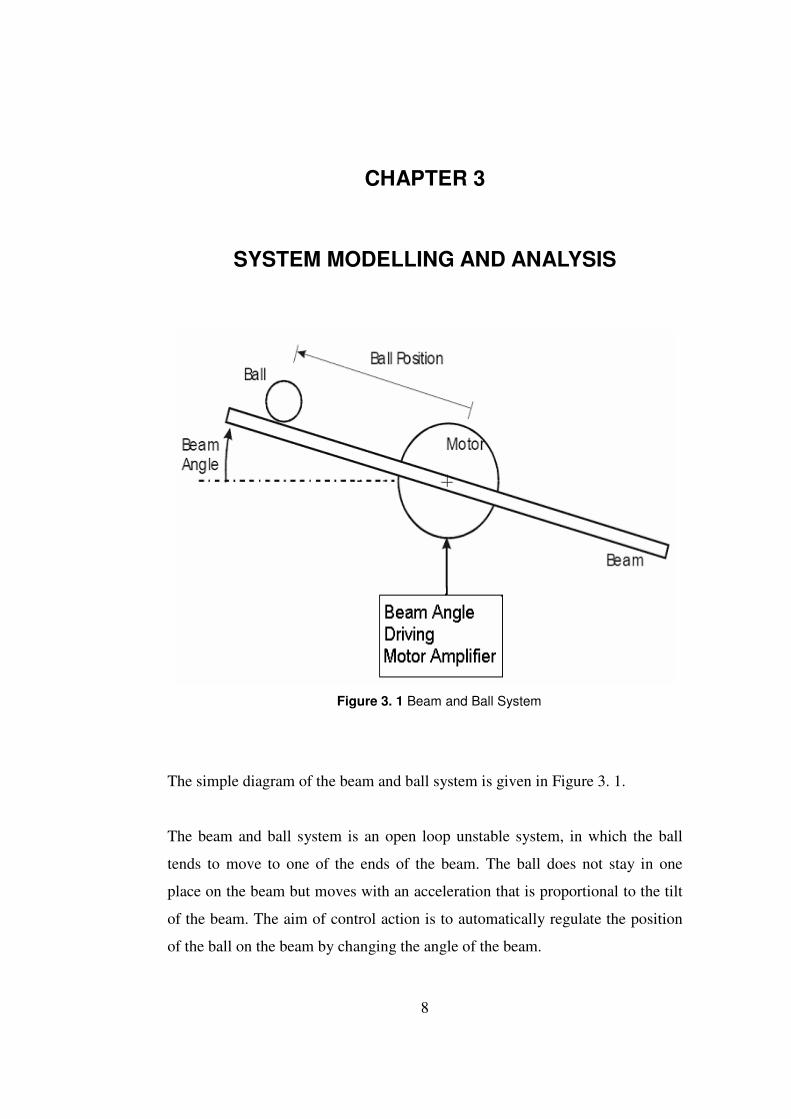
Figure 3. 1 Beam and Ball System
The simple diagram of the beam and ball system is given in Figure 3. 1.
The beam and ball system is an open loop unstable system, in which the ball
tends to move to one of the ends of the beam. The ball does not stay in one
place on the beam but moves with an acceleration that is proportional to the tilt
of the beam. The aim of control action is to automatically regulate the position
of the ball on the beam by changing the angle of the beam.

9
There are physical constraints on the ball position and beam angle. For our
system, the position of the ball can be changed in the range of
mxm 323.0323.0 ≤≤− which is the result of physical beam length. The beam
can be rotated in the range of o4.43≤θ which is the result of beam length and
base hight.
3.1 THE MATHEMATICAL MODEL OF THE SYSTEM
The body diagram of the beam and ball system is given in Figure 3.2. The
system configuration parameters are also given below;
x = Position of the ball, (m)
θ = Rotation of the beam with respect to an inertial frame, (rad)
Φ = Rotation of the ball with respect to an inertial frame, (rad)
m = Mass of the ball, (kg)
MB = Mass of the beam with respect to the center of gravity at point Q,
(kg)
J = Moment of inertia of the ball, (kgm²)
JBp = Moment of inertia of the beam about the pivot P, (kgm²)
τ = Input torque, (Nm)

10
Figure 3. 2 Body Diagram of the Beam and Ball System

11
(refer to Construction and Control of Beam and Ball System by Yüksel Serdar
[17])
Let→
i ,→
j , →
k be the unit vectors corresponding to the coordinate axes at P which
rotate with the angular velocity →•
kθ . The derivatives of the unit vectors →
i and
→
j are;
→•→
+=•
ji θ (3.1.1)
→•→
−=•
ij θ (3.1.2)
Assuming x and y are the coordinates of the center of the ball O with respect to
the rotating frame, its kinematics can be worked out by writing the position
vector →
R with respect to the point P as
→∗∗
→
++=+= jrhxiyjxiR )( (3.1.3)
→•∗∗
••→
+
+−=
•
jxirhxR θθ )( (3.1.4)
→∗∗
•••••→•∗∗
••••→
+−++
−+−=
••
jrhxxixrhxR )(2)(22
θθθθθ (3.1.5)

12
Since the ball rolls without slipping on the wire, its motion can be described as a
rotation of the ball about an axis through its center plus the translation of the
axes along the beam. So, there are two motions coupled: the translational
velocity V, the rotational velocity W.
Then, the velocity of the point C of the ball in contact with the wires is;
rotationalnaltranslatio VcVcVc→→→
+= (3.1.6)
−×
+=→
∗•→→
•
jrkRVc φ (3.1.7)
→•→•∗∗∗
••→
+
++−= jxirrhxVc θφθ )( (3.1.8)
The velocity of the point C’ on the wire coincident with C is given as
rotationalnaltranslatio cVcVcV→→→
′+′=′ (3.1.9)
•→•∗
→
′
•→
+−=×=′ θθθ xihRkcV C (3.1.10)
0=′→
trcV (3.1.11)
→∗
→
′ += jhxiRC (3.1.12)

13
Because the rolling takes place without slipping,
→→
′= cVVc , it means
−=••
∗•
φθrx (3.1.13)
As can be seen from Figure 3.2, the force vector acting on the ball is;
( ) ( )→→→
−+−= jmgFnimgFtF θθ cossin (3.1.14)
Using the Newton’s second law of the motion;
••→
= RmF (3.1.15)
( )
−+−=−
•∗∗
•••• 2
sin θθθ xrhxmmgFt
(3.1.16)
( )
+−+=− ∗∗
•••••
rhxxmmgFn
2
2cos θθθθ (3.1.17)
For the rotational motion, Newton’s second law changes into;

14
••→
= φτ J . (3.1.18)
By applying this equation about the center of the ball O, gives;
)(*→→→→••→
+−== jFiFxjrkJ ntφτ (3.1.19)
then
→••
= kJkrFt φ* or ••
= φJrFt * (3.1.20)
Lastly, the moment of inertia of the ball, J is given as
5
2 2mr
J = (3.1.21)
Differentiating both sides of equation (3.1.13), one obtains;
−=
••••••
*r
xθφ (3.1.22)

15
Substituting both equation (3.1.21) and (3.1.22) into equation (3.1.20), one gets;
−
=
∗
••••
∗r
x
r
mrFt θ
5
2 2
(3.1.23)
Taking the moments about P, one obtains;
θτ singhMFthFnx B++− ∗ (3.1.24)
••
= θτ BPJ (3.1.25)
On substituting for Ft and Fn from (3.1.23) and (3.1.24) into (3.1.16) and
(3.1.17), the nonlinear equations given below are obtained;
05
2sin1
5
2 22
2
2
=
++−+−
+
••∗∗
∗
•••
∗θθθ rh
r
rgxx
r
r (3.1.26)
( ) ••∗
∗
•∗∗
••
••••∗
∗
++−+
+−+
−=
xmhr
rxrhmxmx
mgxghMmxmhr
rJ BBP
2
22
22
5
22
cossin5
2
θθ
θθθθτ (3.1.27)

16
Defining state variables as: 1x is the position of the ball, 2x is the angle of the
beam, 3x is the velocity of the ball and 4x is the angular velocity of the beam,
i.e.
•
•
=
=
=
=
θ
θ
4
3
2
1
x
xx
x
xx
(3.1.28)
the system equations can be transformed into the form given below;
( )τ,xfx =•
(3.1.29)
( )xgy = (3.1.30)

17
( )[ ]
[ ]
[ ]
[ ]
+−
++
++
−
+
+−−+++
==
+
+−+
++
−
+−
+
++−−+++
==
=
=
•••
•••
•
•
2
1*
*
2
2*
2*
2*
2**
*
2
*
2*
22
412
2*
2
43121
2
31**
2
4
2*
22
1*
*
2*
2*
2**
*
2
4
2
41
2
1*
*
2
**
*
2
43121
2
41**
2
3
42
31
5
2
15
2
5
2
5
2
5
2
15
2)(
15
2
5
2
5
2
5
2
5
2
5
22
mxmhr
rJ
r
rmh
r
rrh
r
r
mhr
rxxgSinx
r
rxxmxCosxmgxxxrhmghSinxM
x
r
rmxmh
r
rJmh
r
rrh
r
r
gSinxxxmxmhr
rJ
rhr
rxxmxCosxmgxxxrhmghSinxM
xx
xx
xx
BP
B
BP
BP
B
τ
θ
τ
(3.1.31)
1xy = (3.1.32)
After calculating the states in terms of the known parameters of the system, a
nonlinear model for the beam and ball system is obtained. Then, the actual
system is linearized for checking the controllability and observability. Also
linear model is used in designing controllers and reduced-order observers.

18
3.2 LINEARIZATION OF THE SYSTEM
Physical parameters of the actual beam and ball system are given in the
Table 3. 1 below for the calculation of the state-space form.
Table 3. 1 Physical Parameters of the Beam and Ball System
Mass of the beam with cog. (center of gravity) at point Q
MB 136.78 x 10⁻³ kg
Mass of the ball m 18.848 x 10⁻³ kg Moment of inertia of the ball J 0.455 x 10⁻⁶ kgm² Moment of inertia of the beam with respect to the pivot P
JBp 4 x 10⁻³ kgm²
Radius of the ball r 8.329 x 10⁻³ m Distance between the cog. (center of gravity) and the pivot P
h 10.2 x 10⁻³ m
Distance between the two points of the ball in contact with the wires
d 13.785 x 10⁻³ m
Distance between the point of the ball in contact with the wire and the pivot P
h* 17.281 x 10⁻³ m
( )( )4/22dr −
r* 4.264 x 10⁻³ m
Substituting the values in the table, the state-space form of the beam and ball
system becomes:
31 xx =•
(3.2.1)
42 xx =•
(3.2.2)

19
+
++−
−+−−
=•
2
1
2
4
3
1431
21
2
412
2
12
30427.000908.0
02196.001884.0000828.0
)cos(00406.000401.0)sin(1849.0)sin(0389.0
x
xxxxx
xxxxxxx
xτ
(3.2.3)
+
+−
−+
=•
2
1
2
41431
212
40427.000908.0
000526.008553.0
)cos(4195.0)sin(0351.02691.2
x
xxxxx
xxx
x
τ
(3.2.4)
The equilibrium point of the system will be calculated before the linearization of
the system. The equilibrium point of the system can be found from the equation
( ) 0, ==•
τxfx with 0=τ .
As it can be easily seen from the state-space equations of the beam and ball
system, origin is an equilibrium point if τ = 0. If the system is linearized about
the equilibrium point, which is the origin, the following equations are obtained:
( ) ( )tButAxtx +=•
)( , (3.2.5)
( ) ( )tCxty = , (3.2.6)

20
( ) τ=
=
tu
xe ,
0
0
0
0
(3.2.7)
where,
−
−−=
∂∂
==
008656.32004.46
0097.34471.0
1000
0100
0xx
fA (3.2.8)
=
∂∂
==
9.249
4185.2
0
0
0x
fB
τ (3.2.9)
[ ]0001=C (3.2.10)
21
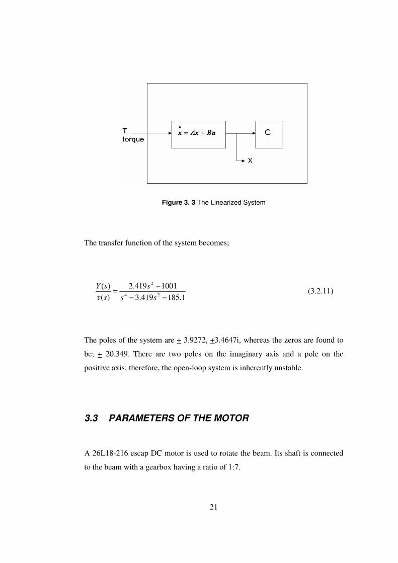
Figure 3. 3 The Linearized System
The transfer function of the system becomes;
1.185419.3
1001419.2
)(
)(24
2
−−
−=
ss
s
s
sY
τ (3.2.11)
The poles of the system are + 3.9272, +3.4647i, whereas the zeros are found to
be; + 20.349. There are two poles on the imaginary axis and a pole on the
positive axis; therefore, the open-loop system is inherently unstable.
3.3 PARAMETERS OF THE MOTOR
A 26L18-216 escap DC motor is used to rotate the beam. Its shaft is connected
to the beam with a gearbox having a ratio of 1:7.

22
Table 3. 2 Parameters of the DC Motor
Terminal resistance R 9.4 Ω Rotor inductance L 0.8 10¯³ H Back EMF constant Kb 0.022 V/rad/s Torque constant Kt 0.022 Nm/A Rotor inertia Jm 8.5 10-7 kgm²
Viscous damping constant Bm 0.4 10-6 N/m/s Terminal voltage V 12 V Maximum continuous torque Tm 0.0163 Nm Maximum continuous current
Ia 0.76 A
The beam and ball system together with DC motor that is used to produce
desired torque is given in Figure 3.4. The motor inductance is neglected because
it is too small as compared to the terminal resistance R. The backlash in the
gearbox, motor inertia and friction are also neglected.
Figure 3. 4 The Linearized System with DC Motor and Gearbox
The input of new linearized model for the beam and ball system is the voltage
applied to the motor, which is V. The output is not changed; it is still the
position of the ball. So the equation between torque and voltage is calculated.
23
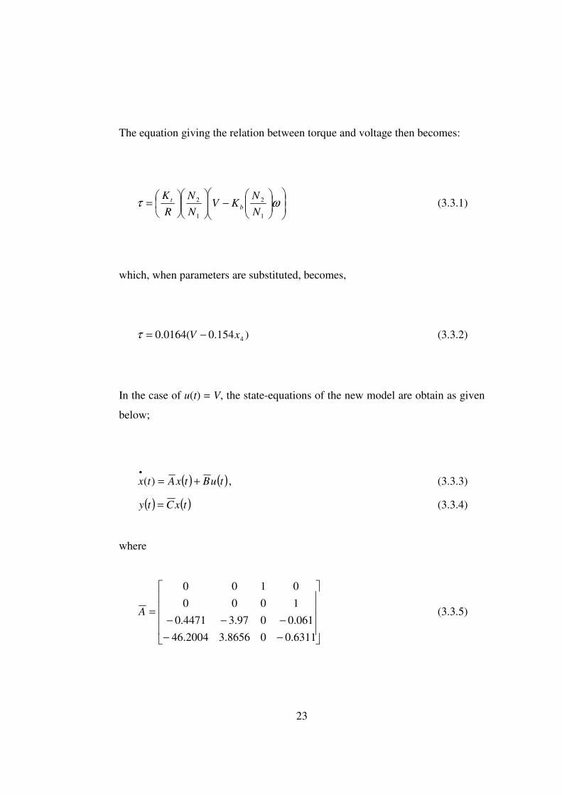
The equation giving the relation between torque and voltage then becomes:
−
= ωτ
1
2
1
2
N
NKV
N
N
R
Kb
t (3.3.1)
which, when parameters are substituted, becomes,
)154.0(0164.0 4xV −=τ (3.3.2)
In the case of u(t) = V, the state-equations of the new model are obtain as given
below;
( ) ( )tuBtxAtx +=•
)( , (3.3.3)
( ) ( )txCty = (3.3.4)
where
−−
−−−=
6311.008656.32004.46
061.0097.34471.0
1000
0100
A (3.3.5)

24
=
0984.4
0397.0
0
0
B (3.3.6)
[ ]0001=C (3.3.7)
By taking voltage applied to motor (V) as the input and the position of the ball
as the output (y), the transfer function changes to;
1.185536.2419.36311.0
42.162249.00397.0
)(
)(234
2
−−−+
−−=
ssss
ss
sV
sY (3.3.8)
The new poles are found to be 3.8046, -4.0681, -0.1838+3.4537i, whereas the
new zeros becomes 23.3692 and -17.7030. The open loop system is still as one
can easily observe, unstable.

25
3.4 DISCRETE TIME MODEL OF THE SYSTEM
The implementation of the system is going to be realized using a computer, in
other words the system is going to be controlled by a computer. For this reason,
discrete time model of the system has to be calculated for both u(t) = V and
u(t) = τ.
Using the solution of continuous time states, and discretizing one obtains;
( ) ( ) ( ) ( ) τττ dBuetxetx
t
t
tAttA
∫−− +=
0
0
0)( (3.4.1)
By taking TKTt += and KTt =0 ;
( ) ( ) ( ) τττdBuekTxeTkTx
TkT
kT
TkTAAT
∫+
−++=+ )( (3.4.2)
If zero order hold is applied with no delay; i.e.
( ) ( )kTuu =τ , TkTkT +≤≤ τ . (3.4.3)
and

26
τη −+= TkT , (3.4.4)
the following equation
( ) ( ) ( ) τττdBuekTxeTkTx
T
TkTAAT
∫−++=+
0
)( (3.4.5)
with the definitions given below;
CH
Bde
e
T
A
AT
=
=Γ
=Φ
∫ ηη
0
(3.4.6)
becomes
( ) ( )( ) ( )kHxky
kukxkx
=
Γ+Φ=+ )1( (3.4.7)
where

27
( ) ( )⋅⋅⋅++++==Φ
!3!2
32ATAT
ATIeAT
( )B
i
TA
i
ii
∑∞
=
+
+=Γ
0
1
!1
By using Matlab and choosing sampling period as T=20ms Φ, Γ and H are
calculated as;
,
10092.00776.09242.0
0008.010794.00087.0
02.00001.0001.10092.0
002.00008.01
−−
−−−
−−
−
=Φ (3.4.8)
,
002.5
4373.0
1.0
001.0
=Γ (3.4.9)
[ ]0001=H (3.4.10)
The eigenvalues of the Φ matrix are 1.0819, 0.9245 and 0.9977 + 0.0692i. As it
is expected, the system is unstable, because one of the eigenvalues of the system
is outside the unit circle and two eigenvalues are on the unit circle and one is
inside the unit circle.

28
The discrete time equation of the system with u(t) = V is obtained in a similar
way, using the equations;
CH
Bde
e
T
A
TA
=
=Γ
=Φ
∫_
0
_
_
ηη (3.4.11)
which results in
( ) ( )( ) ( )kxHky
kukxkx
=
Γ+Φ=+ )1( (3.4.12)
Choosing sampling period as T=20ms again and using Matlab one gets:
,
10092.00772.09185.0
002.010794.0008.0
0199.00001.0001.10092.0
002.00008.01
−−
−−−
−−
−
=Φ (3.4.13)
,
081.0
000841.0
0016.0
0
=Γ (3.4.14)
[ ]0001=H (3.4.15)

29
The eigenvalues of the Φ matrix are 1.0766, 0.9224 and 0.995 + 0.0673i. As it
is expected, the system is unstable, because one of the eigenvalues of the system
is outside the unit circle and two eigenvalues are on the unit circle.
3.5 CONTROLLABILITY AND OBSERVABILITY
PROPERTIES OF THE SYSTEM
The controllability analysis of the system is done for continuous time system
with torque input (u(t) = τ). System dynamics is changed when voltage input
(u(t) = V) applied to the system, but the controllability and observability are not
effected. For this reason controllability and observability analysis for voltage
input are not repeated. Also controllability analysis is repeated for discrete time
system with torque input (u(k) = τ), too.
Using the controllability matrix definition;
[ ]BABAABBQ32= , (3.5.1)
controllability matrix of the continuous-time system with u(t) = τ becomes;

30
−
−
=
02778.85409.249
01843.99304185.2
2778.85409.2490
1843.99304185.20
CQ
Since CQ is full rank ( 1010*2631.2)det( −=CQ ), the continuous-time system
with u(t)=τ is completely controllable.
For the discrete time system, if we use the controllability matrix definition
[ ]ΓΦΓΦΦΓΓ= 32DQ , (3.5.2)
the controllability matrix of the discrete-time system with u(t) = τ is found to be:
=
0104.50075.50048.5002.5
3774.04054.04253.04373.0
4005.03003.02001.01.0
0259.0018.00097.0001.0
DQ
Since DQ is full rank ( 710*3502.6)det( −−=DQ ), the discrete-time system with
u(t) = τ is said to be completely controllable.
Only two of four states ( 1x and 2x ) are measured directly, the other two states
( 3x and 4x ) must be estimated. The observability matrix for the continuous-
time system is:
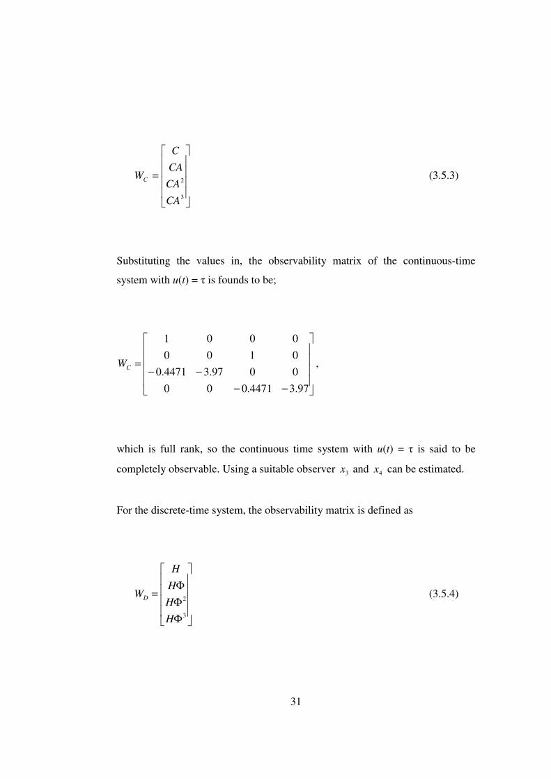
31
=
3
2
CA
CA
CA
C
WC (3.5.3)
Substituting the values in, the observability matrix of the continuous-time
system with u(t) = τ is founds to be;
−−
−−=
97.34471.000
0097.34471.0
0100
0001
CW ,
which is full rank, so the continuous time system with u(t) = τ is said to be
completely observable. Using a suitable observer 3x and 4x can be estimated.
For the discrete-time system, the observability matrix is defined as
Φ
Φ
Φ=
3
2
H
H
H
H
WD (3.5.4)
32
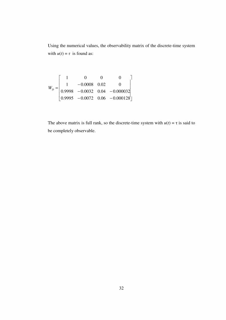
Using the numerical values, the observability matrix of the discrete-time system
with u(t) = τ is found as:
−−
−−
−=
000128.006.00072.09995.0
000032.004.00032.09998.0
002.00008.01
0001
DW
The above matrix is full rank, so the discrete-time system with u(t) = τ is said to
be completely observable.

33
CHAPTER 4
CONTINUOUS TIME CONTROLLER DESIGN AND SIMULATION
4.1 INTRODUCTION
In chapter 3, the modeling of the beam and ball system is given. Using the
models of original system and its linearized version, three different continuous
time controllers are designed and their simulation results are given in this
chapter. The three controllers are based on the following methods;
• State-Feedback
• Computed Torque Method
• Input Based Sliding Mode Controller
4.2 STATE FEEDBACK
The linearized beam and ball system is completely controllable, so the closed
loop poles can be placed at any desired location. Block diagram of the state
feedback is shown in Figure 4. 1.

34
Figure 4. 1 State Feedback Block Diagram
The control law is taken to be;
[ ] )(
)(
)(
)(
)(
)()(
4
3
2
1
4321 tr
tx
tx
tx
tx
kkkktKxtu +
−=−= (4.2.1)
)()( 4321 trkxkkxktu +−−−−=••
θθ (4.2.2)
where K is the state feedback gain matrix. Substituting equation (4.2.1) in
equation (3.4.7) and (3.4.8), one gets;
)()(
)()()()(
tCxty
tBrtxBKAtx
=
+−=•
(4.2.3)

35
where r(t) = 0 is taken for the unforced beam and ball system.
The stability of the system is determined by the eigenvalues of the matrix
)( BKA − . If eigenvalues of )( BKA − matrix are on the left hand side, then no
matter what the initial conditions are the ball approaches to the middle of the
beam (equilibrium point) from the starting point.
To find the feedback gain matrix K, we have to decide what the desired pole
locations are. In this study it is assumed that the closed loop system will have
two negative real roots far away from the dominant roots and two complex
conjugate negative dominant roots that satisfy certain settling time and damping
ratio characteristics. The desired closed loop poles are chosen as;
iS 6.25.12,1 ±−=
5.74.3 −=S
2,1S are the pair of dominant poles and 4.3S are located far away, to the left of
the 2,1S as seen in Figure 4.2. The dominant poles give a characteristic equation
which is 932 ++ ss , indicating a settling time sec67.25.1
44===
n
stξω
and
the damping ratio of 5.0=ξ . With the above mentioned root locations, the
desired characteristic equation becomes
25.50675.30325.11018 234 ++++ ssss . The gain that will result in the above
Characteristic Equation is found to be:
K = [-42.13 27.15 -18.08 4.41];

36
2,1SWn =
Figure 4. 2 Poles of Continuous Time System for State Feedback
The simulation diagram of the overall control system (system with state
feedback) is shown in Figure 4. 3.

37
Figure 4. 3 Simulation Model of Overall State-feedback Control System
The subsystem named “Plant” represents the actual nonlinear beam and ball
system with torque input and the subsystem named “torque” represents the
equation 3.4.4 which is the relationship between voltage and torque. The
controller is designed with respect to voltage input, for this reason the
transformation from voltage to torque equation is used.
The simulation results for two different initial conditions are given in Figure 4.
4 and Figure 4.Figure 4. 45, respectively. It can be seen from figures that the
system reaches to the desired value in a time interval between 2.5-3 second,
which is nearly equal to the settling time.

38
Figure 4. 4 System Response with x(0) = 0.2 m and θ(0) = 0.3 rad (State-feedback)
Figure 4. 5 System Response with x(0) = -0.2 m and θ(0) = 0.3 rad (State-feedback)

39
4.3 CONTROL LAW PARTITIONING
In this section, a second type of controller, using the control law partitioning
method is designed for the nonlinear system.
The torque equation of the nonlinear system as obtained in equation (3.1.27) is;
[ ]2
2
000414.00377.0)cos(1849.0
)sin(0137.0018848.0004.0000413.0
•••
••
••
−++
−
+=
θθθ
θθ
τ
xxxx
xx
(4.3.1)
The system is first brought into the the form βθ
ατ +
= ••
••
x where α and β
depends on system parameters and state variables.
Observing equation (4.3.1), one can define:
[ ]2018848.0004.0000413.0 x+=α , (4.3.2)
and

40
2
000414.0
0377.0)cos(1849.0)sin(0137.0
•
••
−
++−=
θ
θθθβ
x
xxx (4.3.3)
The first part of the control law can be described as β part, which is the part that
linearizes the nonlinear system. The second part of the control law is error
driven in that it forms error signal by differencing desired and actual variables
and multiplies these errors by gains. The error driven portion of the control law
is sometimes called the servo portion. It will be observed that it is a kind of
proportional-derivative (PD) controller.
Define,
τθ
=
••
••
x , (4.3.4)
then the model based portion of the control appears in a control law of the form
βτατ += (4.3.5)
Consider that a complete description of the desired states and its first two
derivatives are available, namely
=
d
d
d
x
θζ ,
= •
••
d
dd
x
θζ and
= ••
••••
d
dd
x
θζ . Using
these definitions the second part of the control law can be written as;

41
)()( ζζζζζτ −+−+=••••
dpdvd kk (4.3.6)
where
=
θζ
x is the actual states, pk and vk are are diagonal matrices giving
the position and velocity gains of the control system, respectively. If these gains
are chosen properly, the dynamic system will be controlled to maintain the
desired state dζ with proper transients performances dictated by pk and vk .
Substituting equation (4.3.4) into equation (4.3.6), one gets;
)()()(0 ζζζζζζ −+−+−=••••••
dPdvd kk (4.3.7)
Defining the error as;
)( ζζ −= de (4.3.8)
and substituting it into Equation (4.3.7), one gets;
ekeke pv ++=•••
0 (4.3.9)

42
Taking Laplace transform of Equation (4.3.9) yields
0)()( 2 =++ sEksks Pv (4.3.10)
It is obvious from Equation (4.3.10) that one can adjust the error dynamics by
choosing proper values for Pk and vk .
The block diagram of the controlled system is shown in Figure 4. 6,
Figure 4. 6 Block Diagram of the Control Law Partitioning
When a damping ratio of 1=ξ and natural frequency of 2=nω is desired. The
pair of dominant poles 22,1 −=s . The constant matrices pk and vk are selected
as diagonal matrices, as follows;

43
−=
4817.1400
08783.96pk
The simulation diagram used to obtain the response of the system using the
controller designed is shown below in Figure 4. 7.
Figure 4. 7 Overall Computed Torque Control System
The subsystem represents the actual nonlinear beam and ball system with torque
input.
−=
81.110
01.108vk

44
The simulation results for two different initial conditions are given in Figure 4.
8 and Figure 4. 89, respectively.
Figure 4. 8 System Response with x(0) = 0.2 m and θ(0) = 0.3 rad (Control law partitioning)
Figure 4. 9 System Response with x(0) = -0.2 m and θ(0) = 0.3 rad (Control law
partitioning)
The comments and conclusions about these results are given in Chapter 7.

45
4.4 SLIDING MODE CONTROL
The sliding mode control input is obtained as a sum of two forms, one which
hold the states on the sliding surface and the other for bringing the states to
sliding surface and back to states on sliding surface. In this section we will first
give a general description of the method.
Assume that an n’th order uncertain linear time invariant system with m inputs
is represented as follows;
),,()()()( uxtftButAxtx ++=•
(4.4.1)
where nxnRA∈ and nxmRB ∈ with nm ≤≤1 .
Generality, it can be assumed that the input distribution matrix B has full rank
which is also true for beam and ball system. (rank(B)=1). The function
nmn RxRRxRf →: is assumed to be bounded by some known functions of the
state. This unknown function includes parameters uncertainty or nonlinearities
present in the system.
The first step of the design is to find an (.)s function. Let mnRRs →: be a
linear function represented by;
xSxs =)( (4.4.2)

46
where mxnRS ∈ is of full rank. Let S be the hyperplane defined by
0)(: =∈= xsRxS n (4.4.3)
The control law is divided into two parts for sliding mode control; equivalent or
linear part of the control law, and nonlinear part of the control law.
The ideal sliding motion can be described as the limiting solution obtained
when the imperfections are removed. In real applications, an ideal sliding
motion is not attainable, because imperfections will result a chattering effect in
a neighbourhood of the sliding surface. The equivalent control is the control
action necessary to maintain an ideal sliding motion on S.
In describing the equivalent control law it will initially be assumed that the
uncertain function ),( uxf is identically zero, i.e the system is given to be in the
form:
)()()( tButAxtx +=•
(4.4.4)
The ideal sliding surface design depends on the property that the system states
lie on the surface S, and an ideal sliding motion takes place at time st .

47
Mathematically this can be expressed as 0)( == xSxs and 0)()( ==••
txSts for
all stt ≥ .
0)()()( =+=•
tBuStAxStxS for all stt ≥ . (4.4.5)
The equivalent control associated with equation (4.4.4), written as equ , is the
unique solution of the algebraic equation 0)()()( =+=•
tBuStAxStxS , namely
)()( 1tAxSBSueq
−−= (4.4.6)
It can easily be seen from equation (4.4.6) that the equivalent control is unique
when )( BS is nonsingular.
When equtu =)( ,
)())(()( 1tAxSBSBItx n
−•
−= . (4.4.7)
But the nominal equivalent control alone is not sufficient to induce a sliding
motion, nominal equivalent control law is just a part of the overall control law.

48
For the second part of the control law, consider the uncertain linear system
given by;
),()()()( xtDtButAxtx ε++=•
(4.4.8)
where the matrix nxlRD ∈ is known and the function ln RxRR →+:ε is
unknown (l is any positive integer). All parameters in the model is related to the
states.
This is a special case of equation 4.4.1, where
),(),( xtDuxf ε= (4.4.9)
Suppose a controller exists which causes a sliding motion on the surface S
despite the presence of the uncertainty. If at time st the states lie on S and
remain there, 0)( =•
ts for all stt > , then the control action is given by;
)),()(()()( 1xtDStAxSBStueq ε+−= − for stt ≥ (4.4.10)
Equivalent control input given in equation (4.4.10) depends on the unknown
parameter ).,( xtε Therefore equation (4.4.10) can not be used in practice. The

49
aim of the equivalent control is to hold system states on S. The following
theorem gives the basis of sliding mode controller.
Theorem: The ideal sliding motion is totally insensitive to the uncertain function
),( xtε in equation (4.4.8) if )()( BRDR ⊂ .
(Refer to “Sliding Mode Control Theory and Applications” by Christopher
Edwards and Sarah K. Spurgeon, Taylor & Francis Ltd, 1998 [18])
An uncertainty which lies within the range space of the input distribution matrix
is described as matched uncertainty.
When matched uncertainty alone is present, it is sufficient to consider the
nominal linear system representation when designing the switching function.
The sliding motion depends on the choice of sliding surface. A convenient way
to solve the problem is to first transform the system into a suitable canonical
form. In this form the system is decomposed into two connected subsystems,
one acting in R(B) and the other in N( S ) (It can be seen from sliding mode
control theory and applications by C. Edwards and S.K. Spurgeon [18] that a
matrix consists of R(B) and N( S ) is linearly independent- Proposition 3.1 and
3.2). If rank(B) = m, there exists an invertible matrix of elementary row
operations nxn
r RT ∈ such that
=
2
0
BBTr (4.4.11)
where mxmRB ∈2 and is nonsingular.

50
This result is applicable to beam and ball system because rank (B)=1=m. rT can
be computed via ‘QR’ decomposition of B matrix. By using coordinate
transformation xTx r↔ the distribution matrix that has the form of equation
4.4.11 can be found. If the states are partitioned so that
=
2
1
x
xx (4.4.12)
where 31 RRx mn =∈ − and 1
2 RRx m =∈ then the nominal linear system given
in equation 4.4.4 can be written as;
)()()( 2121111 txAtxAtx +=•
(4.4.13)
)()()()( 22221212 tuBtxAtxAtx ++=•
(4.4.14)
This representation is referred to as regular form. The first equation above
describes the null space dynamics and second equation above describes the
range space dynamics. If the sliding function matrix in this coordinate system is
partitioned as;
= 21 SSS (4.4.15)

51
where )(1
mnmxRS −∈ and mxmRS ∈2 , the necessity and sufficient condition for
the matrix )( BS to be nonsinular is that 0)det( 2 ≠S and 0)det( 2 ≠B .
( )det()det()det()det( 2222 BSBSSB == ).
During ideal sliding, the motion is given by
0)()( 2211 =+ txStxS for all stt ≥ (4.4.16)
One can formally express )(2 tx in terms of )(1 tx
)()( 12 tMxtx −= for all stt ≥ (4.4.17)
where
1
1
2 SSM−= (4.4.18)
)()()( 112111 txMAAtx −=•
(4.4.19)
Two results are obtained using the equations written above; the matrix 2S has
no direct effect on the sliding motion and acts only as a scaling factor for the
switching function and, the matrix MAAAs
121111 −= must have stable
eigenvalues.

52
The hyperplane design problem boils down to choosing a state feedback matrix
to meet the required performance of the reduced order system ( 1211 , AA ).
Provided the pair (A,B) is controllable, the pair ( 11A , 12A ) is controllable and
any robust linear state feedback method can be applied to designing M. (proves
can be found from Sliding mode control theory and applications by C. Edwards
and S.K.Spurgeon)
For the beam and ball system the number of states (n) is 4 and the number of
control input (m) is 1. Using Matlab, rT is computed via “QR” decomposition of
B matrix.
,rT ,11A ,12A ,21A 22A and 2B matrices are found as using (3.2.8) and (3.2.9);
−−
−
−−=
1011.000
00013.0011.001
011.010011.0
0010
rT ,
−
−
−
=
− 057.01041
012.400035.0057.0
011.000
6
11
x
A
−
−
=
000645.0
0455.0
1
12A
−= 811.345.42043.021A [ ]587.022 −=A

53
092.42 −=B .
When the desired n-m sliding mode poles are selected as -2, -2 and -10 (which
are the poles of MAAAs
121111 −= matrix), the sliding surface matrix S and M
becomes,
[ ]12.147.10575.1325.45 −−=S
[ ]36.4597.9575.13 −−=M
When the nominal equivalent control is equal to state feedback control law, the
state feedback control gains are calculated using equation 4.4.6 as;
[ ]163.3057.1121.1137.10 −−=eqK
After finding the first part of the control input, the second part of the control
input design procedure will be explained.
It is necessary that in a certain domain enclosing the surface, the trajectories of
s(t) must be directed towards it. This may be expressed mathematically as;
)(txKu eqeq −=

54
0lim0
<•
→ +s
s and 0lim
0>
•
→ −s
s (4.4.20)
The equation 4.4.20 is often replaced by;
0<•
ss (4.4.21)
or practically;
sss η−<•
(4.4.22)
where η is a small positive constant.
Equations 4.4.21 and 4.4.22 are termed as reachability condition and η
reachability condition, respectively.
The control structures is calculated as equivalent input ( equ ) and a nonlinear or
discontinuous component. Consider an n’th order single input uncertain system
represented by;
)()())(()( tbutxtAAtx per ++=•
(4.4.23)

55
where the nominal pair (A,b) is controllable and )(tAper is a time varying
matched uncertain matrix. In an appropriate coordinate system the pair (A,b) can
always be written in controllable canonical form.
When (A,b) is in the controllable canonical form, the characteristic equation of
the matrix A is given as;
0...... 121 =++++ −
aaan
n
n λλλ
where ia ’s are the last row element of matrix A.
For the beam and ball system where n=4 and m=1, the M matrix can be a row
vector of order n-1 when the pair ( 1211 , AA ) is converted to controllable
canonical form, the characteristic equation of ( MAA 1211 − ) is as follows;
0.... 122
11 =++++ −
−−
mmmn
n
n λλλ (4.4.24)
where ].....[ 11 −= nmmM .
If 12 =S is selected then [ ]2SMS = , and
n
n
i
ii xxmxs +=∑−
=
1
1
)( (4.4.25)

56
where ix represents the i’th component of the state x.
If the pair (A,b) is in the controllable canonical form and uncertainty in the
system is matched, derivatives of the states are as follows;
)()( 1 txtx ii +
•
= for i = 1, …..,n-1 (4.4.26)
)()())(()(1
tutxtatx ii
n
i
in +∆+−= ∑=
•
(4.4.27)
)(ti∆ terms which are coming from equation 4.4.8, are the state related
components of ),( xtDε .
It will be assumed that, for all t, the perturbations )(ti∆ , which constitute the
matched uncertainty, satisfy
+− <∆< iii ktk )( for i =1,2,…..,n for some fixed scalars +ik and −
ik
A common control structure is then
)()()( tututu nl += (4.4.28)

57
where )(tul is a state feedback law (often the nominal equivalent control equ )
and )(tun is the discontinuous or switched component.
If )(tun is selected as follows;
)sgn()(1
sxktun
i
iin η−=∑=
(4.4.29)
where
<
>=
+
−
0
0
ii
ii
i
sxifk
sxifkk (4.4.30)
and η is a small positive scalar coming from η reachability condition, then;
sstktsxss ii
n
i
i ηη −≤−∆−=∑=
•
))(()(1
(4.4.31)
which satisfies the η reachability condition. (Proofs can be seen from Sliding
Mode Control theory and applications by C. Edwards and S.K.Spurgeon [18])
Lastly, ik and η values selected for the calculation of the discontinuous or
switched component of the input;

58
−ik and +
ik are selected using the β which is given in equation 4.3.3.
2
000414.00377.0)cos(1849.0)sin(0137.0•••
−++−= θθθθβ xxxx
5.05.0 ≤≤− β
then +− <∆< iii ktk )( are selectes as;
5.0−=−ik , 5.0=+
ik and 001.0=η .
The overall control system is then given by;
Figure 4. 10 Overall Sliding Mode Control System

59
The plant represents the actual nonlinear beam and ball system with torque
input. G is the state feedback gain of the system. Switched components are
added to the stated feedback gain and the output is fed to the system.
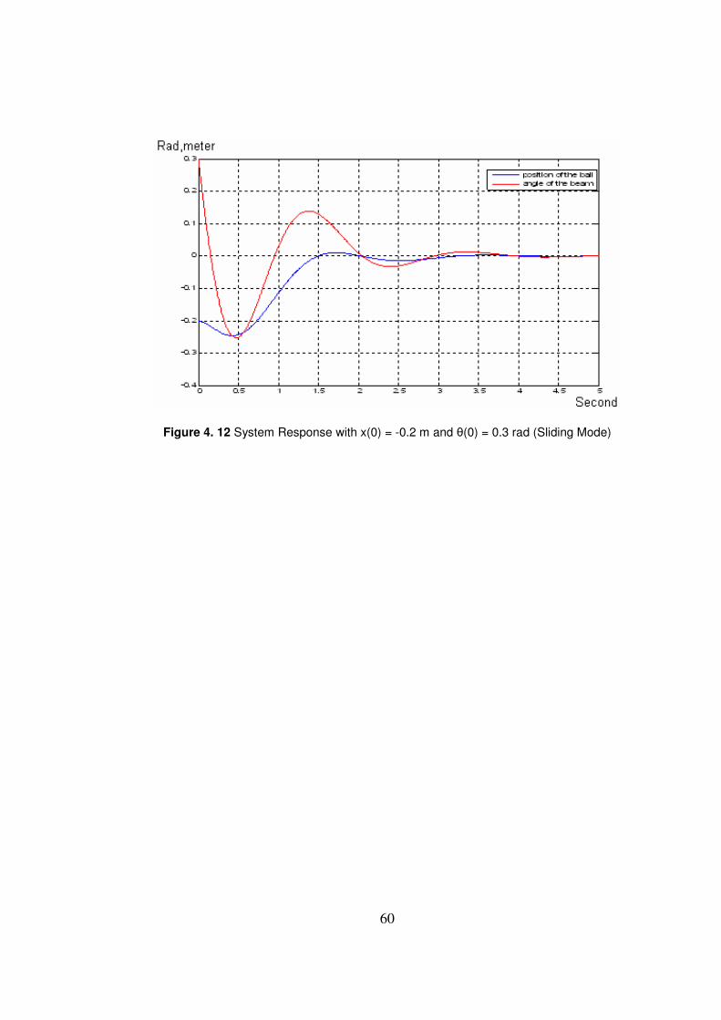
The simulation results for two different initial conditions are given in
Figure 4. 11 and Figure 4.12, respectively.
Figure 4. 11 System Response with x(0) = 0.2 m and θ(0) = 0.3 rad (Sliding Mode)
60
Figure 4. 12 System Response with x(0) = -0.2 m and θ(0) = 0.3 rad (Sliding Mode)

61
CHAPTER 5
DISCRETE TIME CONTROLLER DESIGN AND SIMULATION
5.1 INTRODUCTION
Chapter 4 of this thesis includes design of different continuous time controllers
and their simulation results for beam and ball system. As the system is going to
be controlled by a computer, it is decided to design a discrete time regulator
using state feedback and control law partitioning methods. Also only two of the
four states are measurable; other two states are estimated using reduced order
observer. In chapter 5, discrete time regulators and reduced order observer
design procedure are explained and simulation results are given. The discrete
time control algorithms are;
• State-Feedback
• Control law Partitioning
5.2 REDUCED ORDER OBSERVER
All state variables are required when controlling system using both state
feedback and control law partitioning methods. Unmeasurable states are angular

62
velocity of the beam and the velocity of the ball. Notice that the unmesurable
states are derivatives of the remaining two measurable states.
The states are defined as: the position of the ball is 1x , the angle of the beam is
2x , the velocity of the ball is 3x and the angular velocity of the beam is 4x ; i.e,
•
•
=
=
.24
13
xx
xx (5.2.1)
Differentiating a state variable to generate another state variable is avoided, as
differentiating of a signal decreases the signal to noise ratio because noise
generally increases more rapidly than the command signal. Therefore, an
observer is used to generate the unmeasurable state variables. In chapter 3, it is
shown that the beam and ball system is observable; therefore the design of
observer will not cause any problem.
There are two basic kinds of estimates of the state x[k];
1. Current Estimate: ^
x [k] based on measurement m[k] up to and including the kth instant.
2. Prediction Estimate: ~
x [k] based on the measurement up to m[k-1]
In this thesis reduced order predicted estimator is used.
Prediction Estimator
A discrete time system can be expressed as;

63
][][
][][]1[
kExkm
kukxkx
=
Γ+Φ=+ (5.2.2)
where m[k] are the states that will be measured.
Taking z transform, one obtains:
)()()( zUzXzzX Γ+Φ= or )()()( 1 zUzIzX ΓΦ−= − (5.2.3)
The observer has two inputs, m[k] and u[k], therefore observer state equation
could be written as;
][][][]1[ kLukGmkFqkq ++=+ (5.2.4)
Or, by taking z transform;
)]()([)()( 1 zLUzGMFzIzQ +−= − (5.2.5)
Let the transfer function matrix from U(z) to Q(z) be the same as that from U(z)
to X(z). Thus;

64
)()()( 1 zUzIzQ ΓΦ−= − (5.2.6)
)(])([)()()( 111 zULzIGEFzIzUzI +ΓΦ−−=ΓΦ− −−−
LFzIzIGEFzII 111 )()]()[[ −−− −=ΓΦ−−− , or
( ) ( ) ( )[ ] ( ) [ ]GEFzIFzIGEFzIFzIFzI −−−=−−−− −−− 111 which when
substituted to previous equation yields
( ) ( )[ ]( ) ( ) LFzIzIGEFzIFzI111 −−− −=ΓΦ−+−−
Simplification will result in;
LGEFzIzI 11 ]([)( −− +−=ΓΦ− (5.2.7)
if one chooses Γ=L , then equation 5.2.7 gives;
GEF +=Φ (5.2.8)
Substituting equation (5.2.8) into equation (5.2.4), together with Γ=L gives;
][][][)(]1[ kukGmkqGEkq Γ++−Φ=+ (5.2.9)

65
Errors in the state estimation process is defined as;
][][][ kqkxke −= (5.2.10)
Using the above definition, and equations 5.2.2 together withy equation 5.2.9
gives;
])[)((]1[ keGEke −Φ=+ (5.2.11)
The error dynamics’ characteristic equation is 0=+Φ− GEzI which the same
as that of the observer.
Choosing, )( GE−Φ asymptotically stable; e[k] will converge to zero for any
initial value of the prediction state. (The estimators are generally used for the
systems whose initial conditions are not known.). Another important point is to
choose observer eigenvalues comparably different than those of closed loop
eigenvalues.
The approach usually is to make the observer two to four times faster than the
closed loop control system. The fastest time constant of the closed loop system
is determined from the system characteristic equation,
( ) 0=Γ−Φ− KzI (5.2.12)
66
The time constants of the observer should be equal to from one fourth to one
half time constants of the closed loop control system.
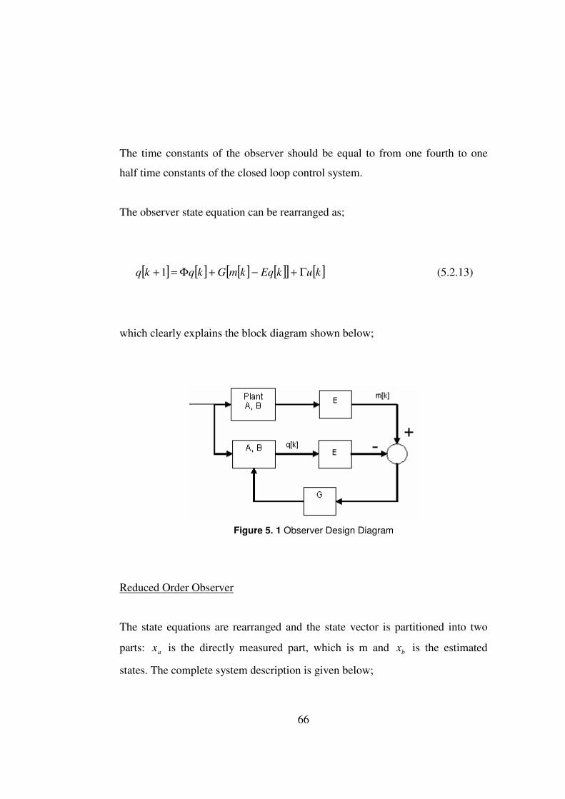
The observer state equation can be rearranged as;
[ ] [ ] [ ] [ ][ ] [ ]kukEqkmGkqkq Γ+−+Φ=+ 1 (5.2.13)
which clearly explains the block diagram shown below;
Figure 5. 1 Observer Design Diagram
Reduced Order Observer
The state equations are rearranged and the state vector is partitioned into two
parts: ax is the directly measured part, which is m and bx is the estimated
states. The complete system description is given below;

67
[ ]
=
Γ
Γ+
ΦΦ
ΦΦ=
+
+
][
][0][
][][
][
]1[
]1[
kx
kxIkm
kukx
kx
kx
kx
b
a
b
a
b
a
bbba
abaa
b
a
(5.2.14)
where
=
2
1
x
xxa , with 1x being the position of the ball and 2x being the angle of the
beam
,4
3
=
x
xxb with 3x being the velocity of the ball and 4x being the angular
velocity of the beam
Consider the first equation obtained from equation 5.2.14;
][][][]1[ kukxkxkx ababaaaa Γ+Φ+Φ=+ (5.2.15)
or equivalently;
][][][]1[ kxkukxkx babaaaaa Φ=Γ−Φ−+ . (5.2.16)

68
All parameters on the left hand side of the equation (5.2.16) are known, or
measured, so the term on the right hand side is known. The second equation
obtained from equation 5.2.14 is
[ ]][][][]1[ kukxkxkx bababbbb Γ+Φ+Φ=+ (5.2.17)
the terms in the square bracket of the equation (5.2.17) [ ]( )][][ kukx baba Γ+Φ are
known.
Then one obtains the reduced order observer equations by making the following
substitutions into the full order observer equations:
ab
aaaaa
baba
bb
b
E
kukxkxkm
kukxku
kxkx
Φ←
Γ−Φ−+←
Γ+Φ←Γ
Φ←Φ
←
][][]1[][
][][][
][][
(5.2.18)
If the substitution given in equation (5.2.18) is made into the equation (5.2.13),
the equation for the reduced order observer can be obtained as;

69
[ ] [ ] [ ] [ ] [ ] [ ]
)(
11^^^
ku
kxkukxkxGkxkx
b
babaaaaabbbb
Γ+
Φ−Γ−Φ−++Φ=+
(5.2.19)
where ^
bx is the estimated values of bx states.
The error equation is found by subtracting equation (5.2.19) from equation
(5.2.17);
[ ] [ ] [ ] [ ] [ ]
Φ−Φ+Φ−Φ=+ kxkxGkxkxke babbabbbbbbb
^^
1 (5.2.20)
or
[ ] [ ] [ ]keGke abbb Φ−Φ=+1 (5.2.21)
Equation (5.2.21) shows that the dynamic behaviour of the error is determined
by the eigenvalues of matrix [ ]abbb GΦ−Φ . If the eigenvalues of the
[ ]abbb GΦ−Φ matrix are in the unit circle, then the error vector will converge to
zero in a finite time for any initial e[0]. The design is then to select a G vector
so that the eigenvalues of matrix [ ]abbb GΦ−Φ are inside the unit circle, and
dynamic behavior of the error vector is asymptotically stable and adequately
fast.

70
The second criterion in designing of the reduced order observer is that the
observer response must be faster than the system response.
The selection of observer gain matrix G is determined by the characteristic root
allocation of matrix [ ]abbb GΦ−Φ . All roots should be inside the unit circle and
the observer response should be faster than the system response.
5.2.1 SIMULATION OF THE STATE FEEDBACK CONTROLLERS WITH REDUCED ORDER OBSERVER
The control law for this controller is;
][][][ krkKxku +−= (5.2.24)
where K is the state feedback gain matrix and ][kr is the reference which is
zero for beam and ball system . Substituting equation (5.2.24) into the system
equation (3.4.7), results in:
][)(]1[ kxKkx Γ−Φ=+ (5.2.25)
The solution of the equation (5.2.25) is;
]0[)(][ xKkx kΓ−Φ= (5.2.26)

71
where x[0] is the initial state. The stability characteristics of the system are
determined by the eigenvalues of the matrix )( KΓ−Φ . So the matrix K must be
chosen to guarantee the asymptotical stability. For this reason the eigenvalues of
the )( KΓ−Φ matrix must be inside the unit circle.
When one chooses, for example, the eigenvalues
861.0
0504.0969.0
4,3
2,1
=
±=
z
iz
the K matrix is calculated as;
[ ]98.396.156.2434.36 −−=K .
Observer response is chosen at least two to five times faster than the system
response. The observer poles in the continuous time domain are chosen as;
is 685.163.72,1 ±−=
Using sTez = with T = 0.02, discrete time pole locations will be chosen as;
iz 199.0835.02,1 ±=
The G matrix for these pole locations is then calculated to be:
−
−=
1215
84G

72
Actual nonlinear system including the DC motor, gearbox, reduced order
observer, state feedback controller gains and low pass filter is shown below.
Figure 5. 2 Overall Discrete Time State Feedback Control System
The simulation results of the system for two different initial conditions are given
in Figure 5. 3, Figure 5. 4. An example observer error plot for initial conditions
[ ]radm 3.02.0− is given in Figure 5. 5.

73
Figure 5. 3 x(0) = 0.2m, θ(0 ) = 0.3rad. with state feedback
Figure 5. 4 x(0) = -0.2m, θ(0 ) = 0.3rad. with state feedback

74
Figure 5. 5 Observer error with x(0) = -0.2m, θ(0 ) = 0.3rad. with state feedback
5.2.2 SIMULATION OF THE CONTROL LAW PARTITIONING CONTROLLERS WITH REDUCED ORDER OBSERVER
The control law for discrete time controller is;
[ ] ][][][ kkkk βτατ += (5.2.27)
with
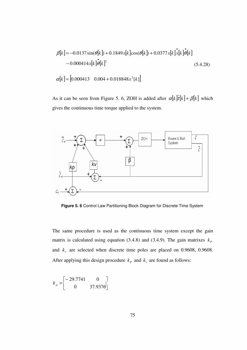
75
[ ] [ ] [ ] [ ] [ ] [ ] [ ]
[ ] [ ]
[ ] [ ]][018848.0004.0000413.0
000414.0
0377.0)cos(1849.0)sin(0137.0
2
2
kxk
kkx
kkxkxkkxkk
+=
−
++−=•
••
α
θ
θθθβ
(5.4.28)
As it can be seen from Figure 5. 6, ZOH is added after [ ] [ ] [ ]kkk βτα + which
gives the continuous time torque applied to the system.
Figure 5. 6 Control Law Partitioning Block Diagram for Discrete Time System
The same procedure is used as the continuous time system except the gain
matrix is calculated using equation (3.4.8) and (3.4.9). The gain matrixes Pk
and vk are selected when discrete time poles are placed on 0.9608, 0.9608.
After applying this design procedure Pk and vk are found as follows:
−=
9376.370
07741.29pk

76
−=
1736.50
05604.23vk
Observer response is designed to be at least two to five times faster than the
system response. The observer poles are chosen as;
2.02,1 =z
Corresponding continuous time poles are both -80.4719.
The G matrix for these pole locations is;
=39.61 0.045-
0.227- 40G
Actual nonlinear system including the DC motor, gearbox, reduced order
observer, state feedback controller gains and low pass filter is given below. The
simulation results of the system with two different initial conditions are given in
Figure 5. 8 and Figure 5. 9. The observer error plot for [ ]radm 3.02.0− initial
conditions is given in Figure 5. 10.

77
Figure 5. 7 Overall Discrete Time Control Law Partitioning Control System
Figure 5. 8 x(0) = 0.2m, θ(0 ) = 0.3rad. with control law partitioning

78
Figure 5. 9 x(0) = -0.2m, θ(0 ) = 0.3rad. with control law partitioning
Figure 5. 10 Observer error with x(0) = -0.2m, θ(0 ) = 0.3rad. with control law
partitioning

79
CHAPTER 6
IMPLEMENTATION
6.1 INTRODUCTION
The hardware of the beam and ball system is illustrated in Figure 6. 1.
Comparing with previous thesis, ball position measurement circuit and beam
angle measurement circuit are redesigned. An advanced version of I/O board to
acquire the voltage and output control signal is used. The power amplifier
circuit is kept as is. The controller software is given in Appendix A, whereas the
connection diagram of the overall system is given in Appendix B.
Computer
& I/O
Board
Power
Amplifier
AngleMeasurement
Circuit
Position
Measurement
Circuit
Power
Supplies
+5V
-5V
Position
Voltage
Angle
Voltage
ControlVoltage
Motor
Encoder
Beam
And Ball
System
Gear
Box
+5V
-15V
GND
+15V
24V
GND
Computer
& I/O
Board
Power
Amplifier
AngleMeasurement
Circuit
Position
Measurement
Circuit
Power
Supplies
+5V
-5V
Position
Voltage
Angle
Voltage
ControlVoltage
MotorMotor
Encoder
Beam
And Ball
System
Gear
Box
+5V
-15V
GND
+15V
24V
GND
Figure 6. 1 Beam & Ball Hardware

80
Photographs of the constructed beam and ball system, sensors and all related
circuits are given in Figure 6. 2.
Figure 6. 2 Beam & Ball System
6.2 BEAM ANGLE MEASUREMENT CIRCUIT
Angle of the beam is measured after a five stage process.
The first stage of the measurement process is composed of an encoder
assembled to the motor. In this thesis HP HEDS 5540F01 type optical encoder

81
is used. Encoder creates 256 pulses per a 3600 full rotation. Motor is connected
to the beam with a 1:7 gear box. So the resolution of the beam angle becomes;
02.00035.07
1*
256
2== rad
π
(6.2.1)
There are three outputs from the encoder CH_A, CH_B and I, each output is
connected to a 5V source with 2.7kΩ pull up resistors as shown in Figure 6. 3 .
Figure 6. 3 Encoder
CH_A and CH_B are 900 phase shifted according to the direction of the
rotation. When the motor turned to left when looking from the aft side, CH_A
leaded CH_B and when motor turned to right CH_B leaded CH_A as seen in
Figure 6. 4. CH_I is connected to get the output signals from CH_A and CH_B.
CH_I output is used in the design. Because CH_A and CH_B are sufficient for
design process.

82
Figure 6. 4 Encoder Output in case of rotation to left looking from the aft side
In the second stage the ouputs of the encoder, CH_A and CH_B, are inverted by
a Hex Schmitt Inverter (54LS14). Inverted signals ACH _ and BCH _ are
connected to a two channel D type flip flop with set and reset (74LS74), to
generate up and down pulses. The working principal of the flip flop is given in
Table 6. 1.

83
Table 6. 1 Working principle of 74LS74
INPUT OUTPUT
DSn DRn nCP nD nQ Qn
L H X X H L
H L X X L H
L L X X H H
DSn DRn nCP nD nQn+1 1+nQn
H H ↑ L L H
H H ↑ H H L
H HIGH voltage level
L LOW voltage level
↑ LOW to HIGH CP transition
Qn+1 state after the next LOW to HIGH CP transition
To generate the up pulse train the first channel of 74LS 74 is used. ACH _ is
connected to the set and BCH _ is connected to clock. To generate the down
pulse train the second channel of 74LS 74 is used. ACH _ is connected to the
clock and BCH _ is connected to set.
As the reset of the flip flop is connected to the 5V (logic high) and D input is
connected to ground (logic low) the working principle in Table 6. 1 is reduced
to the conditions given in Table 6. 2.

84
Table 6. 2 Reduced working principle
INPUT OUTPUT
DSn DRn nCP nD nQ Qn
L H X X H L
DSn DRn nCP nD nQn+1 1+nQn
H H ↑ L L H
The generation of the up and down pulses can be better seen in Figure 6. 5.
CH_A
CH_B
CH_A
CH_B
Up Pulse Train
(Q of First channel)
Down Pulse Train
(Q of second channe)
A B C D
CH_A
CH_B
CH_A
CH_B
Up Pulse Train
(Q of First channel)
Down Pulse Train
(Q of second channe)
CH_A
CH_B
CH_ACH_A
CH_BCH_B
Up Pulse Train
(Q of First channel)
Down Pulse Train
(Q of second channe)
A B C D
Figure 6. 5 Generation of UP and DOWN pulse trains
In section A the motor rotates to the left from the aft, in section B motor
changes the rotation direction, in section C motor rotates to the right from aft, in
section D motor again changes the rotation direction.
85
In the third stage the Up and Down pulse trains are counted by three 4–bit
counters (74LS193). The counter 74LS193 is a 4 bit up down counter. The up
and down pulse trains are supplied to the counters from two different inputs. In
the beam and ball setup the capability of the beam rotation can be with in -430
and 430. So the maximum expected rotation of the motor is ±3010. This means
maximum ±214 pulses are needed to be counted down. As seen the required
capability for the counter circuit should be minimum 9 bits. In the circuit design
a 10 bit D/A converter is used. So the counter circuit is designed as 10 bit
counter. To get the 10 bit counter three, 4 bit counters are connected. Three
counters have a capablty to supply 12 bit info but the the two most significant
bits are not used. The borrow of the first counter connected to the down count
input of the second and the overflow of the first counter connected to the up
count input of the second. Also the borrow of the second counter is connected to
the down count input of the third and the overflow of the second counter
connected to the up count input of the third counter.
In the fourth stage the counted digital info is converted to an analog voltage by
the combination of AD561 digital to analog converter and AD847 Operational
amplifier. The D/A conversion from the counted values to analog voltage circuit
is shown in Figure 6. 6.

86
+
+
DI[9..0]
AD847
5K
2.5K
1.65K
2.5V
16
15
2
Va+
+
10
AD561
I
+
+
DI[9..0]
AD847
5K
2.5K
1.65K
2.5V
16
15
2
Va+
+
10
AD561
I
Figure 6. 6 D/A Conversion Circuit
The AD561 10 bit D/A converter generates current proportional with the digital
data. This current is converted to an output voltage by an operational amplifier.
The equation for the current drawn by AD561 is;
[ ]0..91024
2DI
mAI = (6.2.2)
[ ] 50..91024
25)
5.2
5.2(5 −
=−= DImA
KK
IKVa (6.2.3)

87
From equation above when [ ]0..9DI is 0, Va is equal to -5V, when [ ]0..9DI is
512 Va is equal to 0V, and when [ ]0..9DI is 1023 ampere Va is nearly equal to
5V.
The measured results are;
[ ]
[ ]
[ ] VVaDI
VVaDI
VVaDI
002.510230..9
014.05120..9
042.500..9
==
−==
−==
(6.2.4)
Equation (6.2.4) indicates that the current of D/A changed proportionally with
2.0108mA rather than 2.0mA. The equations will be;
[ ] 042.50..91024
0108.25 −
= DImA
KVa (6.2.5)
[ ] 042.50..9*009818.0 −= DIVa (6.2.6)
As the resolution of the encoder is 256 pulses per a full rotation, 511 means
718.593750. The relation between the digital input and the motor angle can be
found as
[ ] ( ) 102359375.718*360
2560..9 +−= MotorAngleDI (6.2.7)

88
[ ]( ) 59375.718256
360*10230..9 +
−= DIMotorAngle (6.2.8)
59375.718)002.5(*48697143.226576 +−= aVMotorAngle (6.2.9)
( )59375.718)002.548697(143.226576*7
1+−= aVBeamAngle (6.2.10)
In the fifth stage the analog voltage is applied to one of the analog input
channels of the I/O board.
The overall circuit for beam angle measurement is shown in Figure 6. 7.
1
1
2
2
3
3
4
4
5
5
6
6
D D
C C
B B
A A
Title
Number RevisionSize
B
Date: 25.12.2007 Sheet of File: C:\Program Files\..\Sheet2.SchDoc Drawn By:
B1
QB2
QA3
DWN4
UP5
QC6
QD7
GND8
D9
C10
LD11
CO12
BRW13
CLR14
A15
VCC16
74LS193
CNT3
B1
QB2
QA3
DWN4
UP5
QC6
QD7
GND8
D9
C10
LD11
CO12
BRW13
CLR14
A15
VCC16
74LS193
CNT1
B1
QB2
QA3
DWN4
UP5
QC6
QD7
GND8
D9
C10
LD11
CO12
BRW13
CLR14
A15
VCC16
74LS193
CNT2
BIT912
OUT22
BIT36
BIT25
BIT47
BIT710
BIT811
BIT69
BIT1013
VDD14
BIT14
REF15
GND3
RFB16
BIT58
OUT11
AD561
DAC
8
32
6
7 4
5
1
AD847OPAMP1
4
CLK3
D2
1
Q5
Q6
CLR
PR
74LS74
DFLPA
10
CLK11
D12
13
Q9
Q8
CLR
PR
74LS74
DFLPB
1 2
74LS14
INVA
3 4
74LS14
INVB
5 6
74LS14
INVC
9 8
74LS14
INVD
11 10
74LS14
INVE
13 12
74LS14
INVF
1 2 3
JP1
CH_A
CH_B
I
147VCC
2.7KR1
2.7KR2
2.7KR3
VCC
VCC
100nFC6
100nFC3
100nFC4
100nFC5
100nFC2
VCC
7
VCC14
VCC
VCC
VCC
VCC
VCC
VCCVCC
VCC
Clear Switch
Zeroize switch
10K
R4
GND
-15V
OFFSET
OUT
-15V
3.3KR6
3.3KR7
100R5
1uFC9 100nF
C10
-15V100R5
1uFC7 100nF
C8
+15V
100nFC11
100nFC1
12
Beam Angle
Figure 6. 7 Beam Angle Measurement Circuit

89
6.3 MEASUREMENT OF THE BALL POSITION
Ball position is measured by using an aluminum rod and a chromo nickel
spring. Aluminum wire is placed to one side of the beam and the spring is
placed on the other side. The metal ball freely rolls on the rod and spring.
Aluminum rod is used to get the output, it has a negligible resistance. Spring is
made up from a chrome nickel wire with 8Ω/m resistance. A 23m long chrome
nickel wire is used for the spring; the final resistance of the wire is 140Ω. The
ball, rod and the spring locations are shown in Figure 6. 8.
Figure 6. 8 Position Sensor
The spring is used as a voltage divider. +5 and -5V are applied to the two ends
of the spring. According to the position of the ball the divided voltage is
transferred to the aluminum rod through the metal ball. As the resistance of the
ball and the aluminum rod are negligible we can assume that there is no voltage
drop. The output voltage proportional with the position of the ball is transferred
to the ball position measurement circuit. The schematic diagram of the circuit
used for the ball measurement s shown in Figure 6. 9.

90
Figure 6. 9 Measurement Cırcuıt for Ball Posıtıon
Because of the composition of the spring, ball may have some disconnections
with the spring when it is rolling on the spring. These disconnections generate
noise on the voltage measured. A low pass filter is designed to eliminate the
noise on the measured voltage. The cut off frequency of the filter is chosen as
50Hz just like the frequency used for the control algorithm. In the final
configuration the filter is composed of 147Ω resistor and 22µF capacitor. The
effect of the low pass filter also is taken into consideration during the
simulations.
The performance of the low pass filter designed could be seen by observing the
difference in Figure 6. 10 and Figure 6. 11.
+5V
-5V
Spring Ball
Aluminium Rod
Designed LPF 50Hz
DAQ LPF
PC
147Ω
22µF
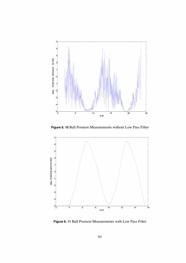
91
0 5 10 15 20 25-5
-4
-3
-2
-1
0
1
2
3
4
5
time
BA
LL P
OS
ITIO
N W
ITH
OU
T F
ILTE
R
Figure 6. 10 Ball Posıtıon Measurements wıthout Low Pass Filter
2 4 6 8 10 12 14 16-5
-4
-3
-2
-1
0
1
2
3
4
5
time
BALL P
OSIT
ION W
ITH F
ILTER
Figure 6. 11 Ball Posıtıon Measurements wıth Low Pass Fılter

92
Some measurements are performed to obtain a mathematical equation between
the ball position and the voltage transfered to I/O card. The voltage
measurements according to the position of the ball are shown in Table 6. 3.
Table 6. 3 Ball position and measured voltage relation
Position of the Ball (m) Voltage measured (V)
-0.323 -4.620
-0,30 -4.410
-0,27 -3,925
-0,24 -3.460
-0,21 -3.045
-0,18 -2.620
-0,15 -2.170
-0,12 -1.747
-0,09 -1.325
-0,06 -0.895
-0,03 -0.487
0 0.0012
0,03 0.428
0,06 0.840
0,09 1.280
0,12 1.716
0,15 2.113
0,18 2.470
0,21 3.000
0,24 3.460
0,27 3.890
0,30 4.340
+ 0.323 4.600

93
As it can be seen from Table 6. 3, the relation is not exactly linear. The relation
between ball position and measured voltage and linear equation based on the
measurements are given in Figure 6. 12.
y = 0,0693x + 0,0018
-0,35
-0,25
-0,15
-0,05
0,05
0,15
0,25
0,35
-5 -3 -1 1 3 5
Series1
Linear (Series1)
Ball Position (m)
Measured Voltage (V)
Figure 6. 12 Ball Posıtıon w.r.t Measured Voltage
After the linearization, the formula for the ball position is obtained as:
Ball Position = 0.0693 * measured voltage + 0.0018 (6.3.1)

94
6.4 POWER AMPLIFIER
The control input leaves the input-output card as an analog signal. Then, it is
applied to the power amplifier the output of which is used to drive the DC
motor. The electrical schematic diagram of the power amplifier circuit is given
in Figure 6. 13.
Figure 6. 13 Power Amplifier Circuit diagram
To perform a bidirectional motor control using a single power supply, which is
24V, a bridge connection with two power operational amplifiers is used.
APEX2S PA21A type operational amplifier had two power opamps in one
package. From Figure 6. 13, the following voltage equations are obtained;
246.9
12
24
8.4
−=−
=
−=
=
VcmdVbVa
Vc
VaVb
VcmdVa
(6.4.1)
Vcmd is the control signal coming from input output card.
Figure 6.13 Power Amplifier Circuit Diagram
From equation (6.4.1), 2.5V command voltage makes both Va and Vb 12V and
results in 0V across the motor. With 1.25V and 3.75V command voltages, (Va -
Vb) becomes -12V and +12V, respectively. This is the full scale voltage range
of the DC motor.

95
As a result, gain of the power amplifier is 9.6 and its input voltage range is
2.5±1.25V. The output range of the I/O board is set to 0 to 5V. The calculated
control input (u=-Kx) for the statefeedback algorithm is rescaled by multiplying
with 1/9.6, and then adding 2.5 in order not to change the closed-loop gain. For
the control law partitioning algorithm the output is found as torque. The torque
is then changed to voltage first and then proceed as is done in the previous case
with voltage.
6.5 PCI-1712 DATA ACQUSITION BOARD
Advantech PCI 1712A advanced multi purpose data acquisition board is used in
this thesis. It is an advanced type of data acquisition board generally used for
industrial processes.
The main features of the board can be given as;
• PCI-bus mastering for data transfer
• 16 single-ended or 8 differential or combination analog inputs
• 12-bit A/D converter, with up to 1 MHz sampling rate
• Pre-, post-, about- and delay-trigger data acquisition modes for analog
input channels
• Programmable gain for each analog input channel
• Automatic channel/gain/SD/BU scanning
• On-board FIFO buffer storing up to 1K samples for A/D and 32K
samples for D/A
• Two 12-bit analog output channels with continuous waveform output
function

96
• Auto calibration for analog input and output channels
• 16 digital Input and output channels
• Three 16-bit programmable multifunction counters/timers on 10MHz
clock.
The board has its own driver and supports high level languages. In the thesis
study mainly two functions of the board are used: A/D conversion and D/A
conversion.
A/D Conversion: The analog inputs, position of the ball and the beam angle are
digitized by the board and used in the control software.
D/A Conversion: The control voltage generates digital control values are
converted to analog voltages and then applied to power amplifier card for
driving the motor.
Some parameters of the board that are used in the thesis study are listed in Table
6.4.

97
Table 6. 4 Used functions of the I/O board
Functions Settings
Card Number 0
Data Acquisition Rate 40000 Hz
Analog output Channels 0
Number of Analog Input Channels 2
Analog input start channel 1
Analog input interval -5V / 5V
Analog Output interval 0V / 5V
Digital to Analog Conversion Rate 500
Timer function period 0.02 sec
Data call back function TimerFcn
6.6 SOFTWARE
The control software is written in MATLAB and explained in Appendix A.
A GUI is designed for the Man machine interface and the control software is
written as an m file. For control law partitioning and state feedback algorithms
two different controller software are written as an m file. The functions of the
data acquisition tool box are used.
The flow chart and the GUI of the software can be seen in Figure 6. 14.

98
Set beam angle to 0 degree
Set counters to 0 degree (512)
Initialization of the I/O board functions
Clear buffer
Analog inputs taken
Ball position and beam angle calculated
Ball position velocity and beam angle velocity calculated
Control voltage output calculated
Program stopped
Data plotted
Wait for the initial conditions
NY
In 50 Hz
Figure 6. 14 Flowchart and GUI
Functions performed when the GUI is loaded and the buttons pressed are all
explained in detail below.
When the GUI is loaded;
All the initial parameters and the parameters that hold the data are initialized. A
device object for the analog input is created. A device object for the analog
output is created. Number of channels for the analog input is set to 2. Used
analog input channels are set. Used analog output channel is set. Input and
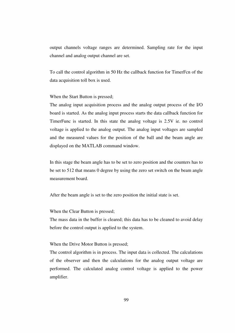
99
output channels voltage ranges are determined. Sampling rate for the input
channel and analog output channel are set.
To call the control algorithm in 50 Hz the callback function for TimerFcn of the
data acquisition toll box is used.
When the Start Button is pressed;
The analog input acquisition process and the analog output process of the I/O
board is started. As the analog input process starts the data callback function for
TimerFunc is started. In this state the analog voltage is 2.5V ie. no control
voltage is applied to the analog output. The analog input voltages are sampled
and the measured values for the position of the ball and the beam angle are
displayed on the MATLAB command window.
In this stage the beam angle has to be set to zero position and the counters has to
be set to 512 that means 0 degree by using the zero set switch on the beam angle
measurement board.
After the beam angle is set to the zero position the initial state is set.
When the Clear Button is pressed;
The mass data in the buffer is cleared; this data has to be cleaned to avoid delay
before the control output is applied to the system.
When the Drive Motor Button is pressed;
The control algorithm is in process. The input data is collected. The calculations
of the observer and then the calculations for the analog output voltage are
performed. The calculated analog control voltage is applied to the power
amplifier.

100
When Put 0 Voltage button is pressed;
The control of the motor is stopped by pressing this button. 0V for the analog
control output is supplied from the control output, now the motor is in the safe
state.
When Stop button is pressed;
Device objects are deleted.
When Plot button is pressed;
All the parameters are saved to file “data_file.mat”.
6.7 EXPERIMENT RESULTS
Some results for stabilized system using control law partitioning and state
feedback methods are given in figures below;

101
0 5 10 15 20 25 30 35 40 45 50-0.3
-0.2
-0.1
0
0.1
0.2
0.3
0.4
Time (sec)
Beam
Angle
(ra
d)
Ball
Positi
on (m
)
Beam Angle
Ball Position
Figure 6. 15 State Feedback
0 5 10 15 20 25 30 35 40 45-0.25
-0.2
-0.15
-0.1
-0.05
0
0.05
0.1
Time
Beam
Angle
Ball P
ositio
n
Beam Angle
Ball Position
Figure 6. 16 State Feedback (teta=-0.2 rad., position=0.14 m.)

102
0 10 20 30 40 50 60 70-0.4
-0.3
-0.2
-0.1
0
0.1
0.2
0.3
Time
Beam
Angle
Ball P
ositio
n
Beam Angle
Ball Position
Figure 6. 17 State Feedback (teta=0.29 rad., position=-0.13 m.)
0 10 20 30 40 50 60-0.5
-0.4
-0.3
-0.2
-0.1
0
0.1
0.2
0.3
0.4
Time
Ball Position
Beam
Angle
Ball Position
Beam Angle
Figure 6. 18 Control Law Partitioning

103
0 5 10 15-0.2
-0.15
-0.1
-0.05
0
0.05
0.1
0.15
0.2
0.25
Time (sec)
Beam
Angle
(ra
d)
Ball
Position (m
)
Beam Angle
Ball Position
Figure 6. 19 Control Law Partitioning (teta=0.23, position=-0.13)
0 5 10 15 20 25 30 35 40-0.1
-0.05
0
0.05
0.1
0.15
0.2
0.25
Time (sec)
Beam
Angle
(ra
d)
Ball Position (m
)
Beam Angle
Ball Position
Figure 6. 20 Control Law Partitioning (teta=0.18 rad., position=0.08 m)
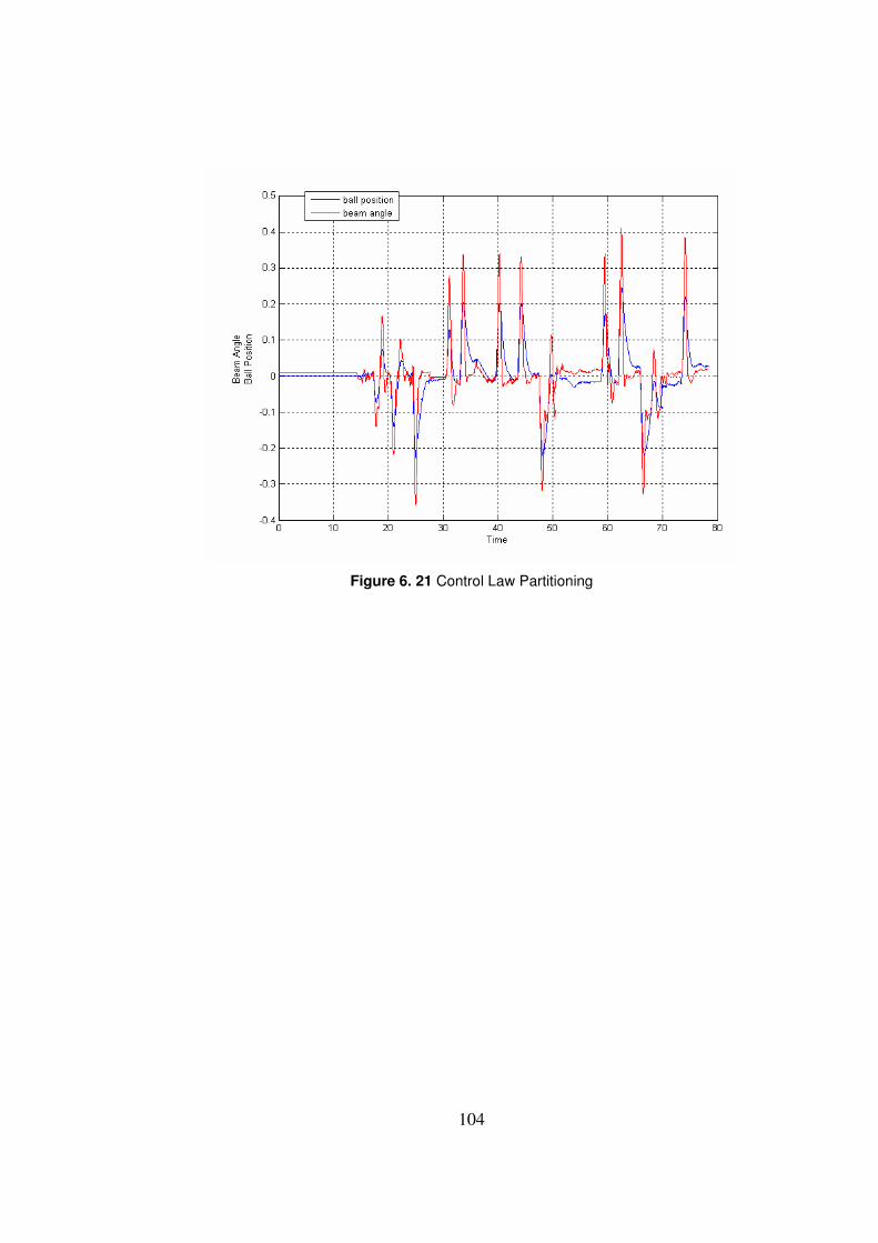
104
Figure 6. 21 Control Law Partitioning

105
CHAPTER 7
RESULTS AND CONCLUSION
In this thesis, three different continuous time controllers are designed and a
control law partitioning with an observer is implemented. In addition a state
feedback controller with an observer which is different from the observer used
for control law partitioning method is also implemented.
There are four states in the system. Two of these states are measurable. They are
position of the ball and angle of the beam; the unmeasurable states are velocity
of the ball and angular velocity of the beam. Unmeasurable states are observed
by using reduced order observer. A spring on the beam is used as a voltage
divider for measuring ball position. However, the output of the position sensor
is too noisy because of the contact problem between ball and wires on the beam.
The contact problem is solved using a low pass filter. An encoder and different
integrated circuits are used for measuring beam position.
Some of the parameters of the system such as backlash in the gear, friction
between ball and wire and nonlinear current torque characteristic of the motor
affect the system response. But these effects are difficult to model so they are
neglected. Another important issue is the initialization of the beam position. It
affects the location of the equilibrium point.
In the remaining part of this chapter performances of different controllers are
evaluated and compared to each other. Some conclusions are given related with
results. Chapter ends with suggestions for future work.

106
Continuous Time Controllers
Three different continuous time controllers are simulated for beam and ball
system; state feedback, control law partitioning and sliding mode control. There
are some advantages and disadvantages of these controllers with respect to each
others.
Required torque for all type of controllers with ball position 0.2m and beam
angel -0.3 rad. are given in Figure 7. 1, Figure 7. 2, Figure 7. 3;
Figure 7. 1 Sliding Mode Controller, required torque versus time

107
Figure 7. 2 Control Law Partitioning, required torque versus time
Figure 7. 3 State Feedback, required torque versus time
The experiment given above is repeated for ball position 0.2m and beam angle
0.3 rad and required torque functions are found as given in Figure 7. 4,

108
Figure 7. 5 and Figure 7. 6;
Figure 7. 4 Sliding Mode Controller, required torque versus time
Figure 7. 5 Control Law Partitioning, required torque versus time

109
Figure 7. 6 State Feedback, required torque versus time
As it can be seen from the required torque graphics given in Figure 7.1 to Figure
7.6, the required torque for state feedback and control law partitioning methods
are close to each other and they are permanent. But required torque for sliding
mode control is temporary and greater than other two methods and chattering
effect can be seen as a result of sliding mode control. The sliding mode plot
shows also the system is approached to sliding surface in a few seconds and on
the sliding surface the required torque is nearly zero. Large value of torque is a
disadvantage of sliding mode controller method. Its advantage is that the
unmodeled parameter effects can be taken into consideration by changing ik
parameters as the theory of the sliding mode controller says.
Maximum required torque for control law partitioning is lower than state
feedback. It is an advantage of control law partitioning over state feedback.
When a state feedback controller designed with settling time 0.6 second and
critical damped ωn is equal to 0.666, required torque is nearly same as control
law partitioning required torque for initial conditions 0.2m and -0.3 rad.
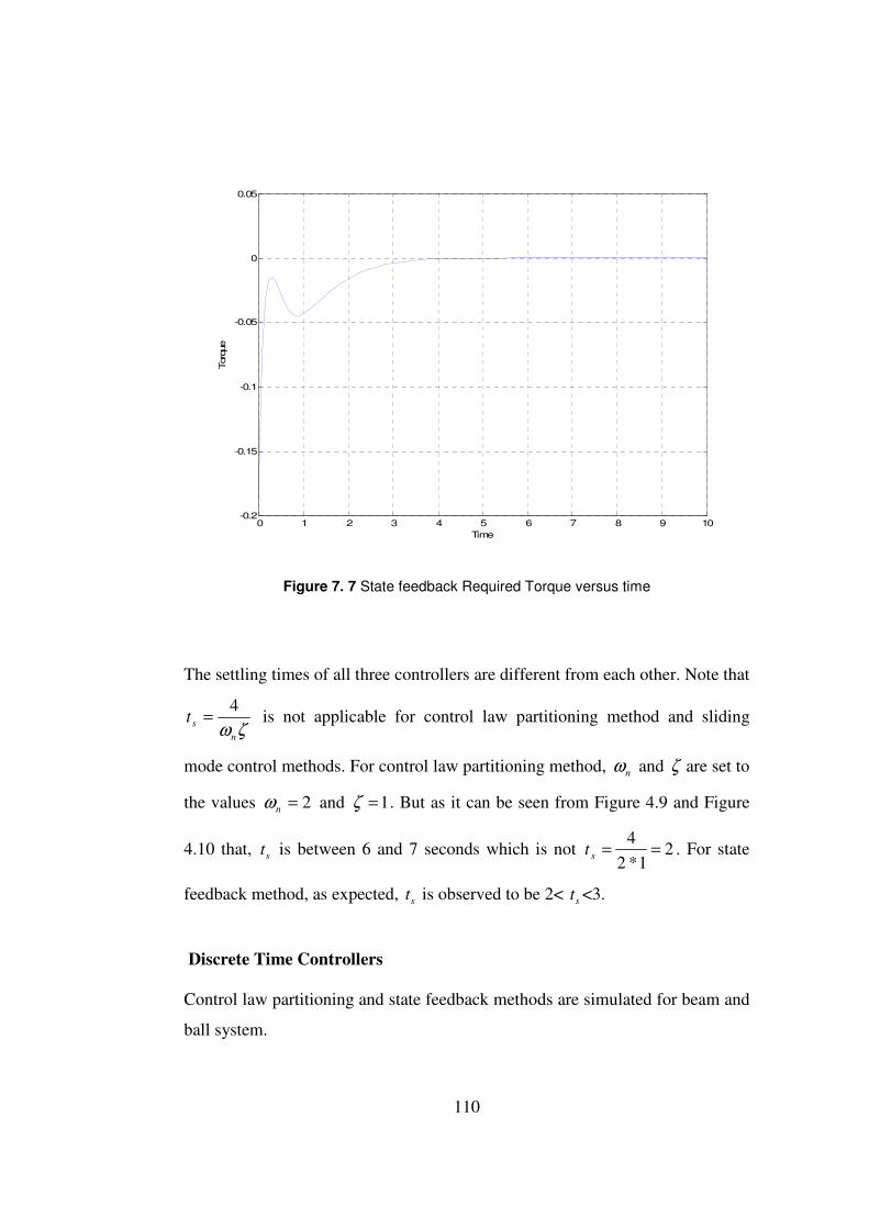
110
0 1 2 3 4 5 6 7 8 9 10-0.2
-0.15
-0.1
-0.05
0
0.05
Time
Torq
ue
Figure 7. 7 State feedback Required Torque versus time
The settling times of all three controllers are different from each other. Note that
ζωn
st4
= is not applicable for control law partitioning method and sliding
mode control methods. For control law partitioning method, nω and ζ are set to
the values 2=nω and 1=ζ . But as it can be seen from Figure 4.9 and Figure
4.10 that, st is between 6 and 7 seconds which is not 21*2
4==st . For state
feedback method, as expected, st is observed to be 2< st <3.
Discrete Time Controllers
Control law partitioning and state feedback methods are simulated for beam and
ball system.

111
For state feedback method, the ball rolls on the beam without dropping when the
initial states are between [-0.25 m, 0.2 rad] and [0.33 m, 0.68 rad.]. Related
voltage, ball position and beam angle versus time plots are given in Figure 7. 8-
Figure 7. 13;
0 0.5 1 1.5 2 2.5 3 3.5 4 4.5 5-15
-10
-5
0
5
10
15
time
voltage
-0.25 meter 0.2 rad
Figure 7. 8 Voltage: State feedback [-0.25m, 0.2 rad]

112
0 0.5 1 1.5 2 2.5 3 3.5 4 4.5 5-0.35
-0.3
-0.25
-0.2
-0.15
-0.1
-0.05
0
0.05
0.1
time
positio
n
-0.25 meter 0.2 rad
Figure 7. 9 Ball Position: State feedback [-0.25m, 0.2 rad]
0 0.5 1 1.5 2 2.5 3 3.5 4 4.5 5-0.5
-0.4
-0.3
-0.2
-0.1
0
0.1
0.2
0.3
time
beam
angle
-0.25 0.2 rad
Figure 7. 10 Beam Angle: State feedback [-0.25m, 0.2 rad]

113
0 0.5 1 1.5 2 2.5 3 3.5 4 4.5 5-15
-10
-5
0
5
10
15
time
voltage
0.33 meter 0.68 rad.
Figure 7. 11 Voltage: State feedback [0.33 m, 0.68 rad.]
0 0.5 1 1.5 2 2.5 3 3.5 4 4.5 5-0.05
0
0.05
0.1
0.15
0.2
0.25
0.3
0.35
time
positio
n
0.33 meter 0.68 rad
Figure 7. 12 Position: State feedback [0.33 m, 0.68 rad.]

114
0 0.5 1 1.5 2 2.5 3 3.5 4 4.5 5-0.4
-0.2
0
0.2
0.4
0.6
0.8
1
teta
time
0.33 meter 0.68 rad
Figure 7. 13 Beam Angle: State feedback [0.33 m, 0.68 rad.]
For control law partitioning method, the ball rolls on the beam without dropping
when the initial states are between [-0.25m, 0.3 rad] and [0.33 m, 0.7 rad].
Related voltage, ball position and beam angle versus time plots are given in
Figure 7. 14 - Figure 7. 19;

115
0 1 2 3 4 5 6 7 8 9 10-12
-10
-8
-6
-4
-2
0
2
time
voltage
-0.26 meter 0.3 rad
Figure 7. 14 Voltage: Control law partitioning [-0.26m, 0.3 rad]
0 1 2 3 4 5 6 7 8 9 10-0.35
-0.3
-0.25
-0.2
-0.15
-0.1
-0.05
0
0.05
time
positio
n
-0.26 meter and 0.3 rad
Figure 7. 15 Position: Control law partitioning [-0.26m, 0.3 rad]

116
0 1 2 3 4 5 6 7 8 9 10-0.4
-0.3
-0.2
-0.1
0
0.1
0.2
0.3
time
teta
-0.26 meter and 0.3 rad
Figure 7. 16 Beam Angle: Control law partitioning [-0.26m, 0.3 rad]
0 1 2 3 4 5 6 7 8 9 10-10
-5
0
5
10
15
time
voltage
0.33 meter and 0.7 rad
Figure 7. 17 Voltage: Control law partitioning [0.33 m, 0.7 rad]

117
0 1 2 3 4 5 6 7 8 9 10-0.05
0
0.05
0.1
0.15
0.2
0.25
0.3
0.35
time
positio
n
0.33 meter and 0.7 rad
Figure 7. 18 Position: Control law partitioning [0.33 m, 0.7 rad]
0 1 2 3 4 5 6 7 8 9 10-0.6
-0.4
-0.2
0
0.2
0.4
0.6
0.8
time
teta
0.33 meter and 0.7 rad
Figure 7. 19 Beam Angle: Control law partitioning [0.33 m, 0.7 rad]

118
Above experiments indicate that when all the system including motor, power
amplifier and observer is simulated, the ranges of controllable initial conditions
for control law partition method is larger than the state feedback method. In
other words, the controller designed using control law partitioning method
controls some initial points which are not controlled by state feedback
method.When it is repeated for state feedback controller with settling time 6
seconds and critical damped, still control law partitioning method ranges of
controllable initial conditions are similar to state feedback method.
Reduced order observer poles for control law partitioning method are placed far
away from the origin with respect to state feedback method. Reduced order
observer poles are iz 199.0835.02,1 ±= when state feedback method is used.
Reduced order observer poles are 2.02,1 =z when control law partitioning
method is used.
The experimental results show that the constructed beam and ball system is
successfully stabilized using both control law partitioning and state feedback. It
is also shown that control law partitioning method is not as sensitive as state
feedback method to the deformation of the beam. Beam is made of a kind of
plastic for this reason it is sensitive for heat changes. When stabilizing the
system by control law partitioning method some deformations of the beam do
not cause instability but same beam condition causes oscillation when the
system is controlled using state feedback method.
Secondly, setting the beam angle other than 0° at the initialization causes the
system to stabilize at a different equilibrium point rather than the origin. The
relation is given in Figure 7. 20;

119
y = 2.9755x + 0.0195
-0.35
-0.3
-0.25
-0.2
-0.15
-0.1
-0.05
0
0.05
0.1
-0.12 -0.1 -0.08 -0.06 -0.04 -0.02 0 0.02
angle
po
siti
on
n
Seri 1
Doğrusal (Seri 1)
Figure 7. 20 Initialization Error
For further study, a sliding mode controller can be applied to the system. The
design criteria of continuous time sliding mode controller and the simulation
results are given in this thesis. The unmodeled parameters effect can be fully
removed using sliding mode controller. The reason for the popularity of this
type of controller is its robustness and its law order.

120
REFERENCES
1) Advantech Co. Ltd., PC –Multilab Card User’s Manual
2) Matlab Data Acquisition Toolbox
3) 74LS14 Datasheet
4) 74LS74 Datasheet
5) 74LS193 Datasheet
6) AD561 Datasheet
7) AD 847 Datasheet
8) PA21 Datasheet
9) HEDS 5540 Datasheet
10) G.F Franklin., J.D Powell., M.L.Workman, “Digital Control of Dynamic
Systems”, Prentice-Hall, 1998, Book
11) R. J. Schilling, “Fundamentals of Robotics Analysis and Control”, Prentice
Hall; 1990, Book.
12) J. J. Craig “Introduction to Robotics Mechanics and Control”, Prentice
Hall; 2nd
edition, 1989, Book.

121
13) C.-T. Chen, “Linear System Theory and Design”, Oxford University Press,
USA; 3rd
edition ,1998, Book
14) G. Monsees, “Discrete-Time Sliding Mode Control”, Technische
Universiteit Delft, 2002, Phd. Thesis
15) C.H. An, C.G. Atkeson and J. M. Hollerbach, “Modal-based Control of a
Robot Manipulator”, Massachusetts Institude of Technology, 1988, Book.
16) D. Kostic, “Data-driven Robot Motion Control Design”, Technische
Universiteit Eindhoven, Netherlands, 2004, Phd Thesis.
17) Y. Serdar, “Construction and Control of a Beam and Ball Experimental
System”, Middle East Technical Univercity, 1998, Ms Thesis
18) E. Christopher, S. K. Spurgeon, “Sliding Mode Control: Theory and
Applications”, Taylor & Francis Ltd, 1998, Book.
19) J. Hauser , S. Sastry, P. Kokotovic, “Nonlinear Control via Approximate
Input-Output Linearization: The Ball and Beam Example”, IEEE
Transactions on Automatc Control, 1992, vol 37, issue. 3, pp. 392 – 398
20) W. Yu, F. Ortiz, “Stability Analysis of PD Regulation for Ball and Beam
System”, Proceedings of IEEE Conference on Control Applications, 2005,
pp. 517 - 522
21) Y. Jiang, C. McCorkell, R. B. Zmood, “Application of Neural Networks for
Real Time Control of a Ball-Beam System”, Proceedings of IEEE
International Conference on Neural Networks, 1995. Vol. 5, pp. 2397 - 2402

122
22) K. C. Ng, M. M. Trivedi, “Neural Integrated Fuzzy Controller (NiF-T) and
Real-Time Implementation of a Ball Balancing Beam (BBB)”, Proceedings
of IEEE International Conference on Robotics and Automation, 1996. Vol.
2, pp. 1590 – 1595.
23) K. C. Ng, M. M. Trivedi, “Fuzzy Logic Controller and Real Time
Implementation of a Ball Ballancing Beam”, SPIE, Orlando, Florida 1995,
pp 261--272 ,
24) G. Cristadoro, A. De Carli and L. Onofri, “A Robust Control Strategy for
an Unstable Mechanical System”, Proceedings of IEEE 4th
International
Workshop on Advanced Motion Control, 1996, Vol. 2, pp. 488 - 493
25) J. Huang, C.-F. Lin, “Robust Nonlinear Control of the Ball and Beam
System”, Proceedings of American Control Conference, 1995, Vol. 1, pp.
306 - 310
26) M. A. Marra, B. E. Boling, B. L. Walcott, “Genetic Control of a Ball -
Beam System”, Proceedings of the - IEEE International Conference on
Control Applications, 1996, pp. 608 - 613
27) R. O. Saber, A. Megretski, “Controller Design for the Beam and Ball
System”, Proceedings of the 37th
IEEE Conference on Decision and
Control, 1998, Vol. 4, pp. 4555 - 4560
28) H. K. Lam, F. H. F. Leung, P. K. S. Tam, “ Design of a Fuzzy Controller
for Stabilizing a Ball and Beam System”, Proceedings of The 25th
Annual
Conference of IEEE Industrial Electronics Society, 1999, Vol. 2, pp. 520 -
524

123
29) F. Mazenc, A. Astolfi, R. Lozano, “Lyapunov Function for the Ball and
Beam: Robustness Property”, Proceedings of the 38th
IEEE Conference on
Decision and Control, 1999, Vol. 2, pp. 1208 - 1213
30) P. H. Eaton, D. V. Prokhorov, D. C. Wunsch, “Neurocontroller Alternatives
for Fuzzy Ball and Beam Systems with Nonuniform Nonlinear Friction”,
IEEE Transactions on Neural Networks, March 2000, Vol. 11, No 2, pp.
423-435.
31) H. S. Ramirez, “On the Control of the Ball and Beam System: A Trajectory
Planing Approach”, Proceedings of the 39th
IEEE Conference on Decision
and Control, 2000, Vol. 4, pp. 4042 – 4047.
32) J. YI, N. Yubazaki, K. Hirota, “Stabilization Control of Ball and Beam
Systems”, IFSA World Congress and 20th
NAFIPS International
Conference, 2001, Joint 9th Vol. 4, pp. 2229 - 2234
33) F. Song, S. M. Smith, “Applying Incremental Best Estimate Directed
Search to Optimize Fuzzy Logic Controllers for Ball and Beam System”,
Proceedings of the IEEE International Conference on Fuzzy Systems, 2002,
Vol. 2, pp. 1132-1137.
34) J. M. Lemos, R. N. Silva, J. S. Marques, “Adaptive Control of the Ball and
Beam Plant in the Presence of Sensor Measure Outliers”, Proceedings of the
American Control Conference, 2002, Vol. 6, pp. 4612 – 4613.
35) S. Sridharan, G. Sridharan, “Ball and Beam on Roller: A New Control
Laboratory Device” Proceedings of the 2002 IEEE International Symposium
on Industrial Electronics, 2002, Vol. 4, pp. 1318 – 1321.”

124
36) R. M. Hirschorn, “Incremental Sliding Mode Control of the Ball and Beam”.
IEEE Transactions on Automatic Control, 2002, Vol. 47, No. 10, pp. 1696-
1700.
37) Y. Guo, D. J. Hill, Z. P. Jiang , “Global Nonlinear Control of the Ball and
Beam System” Proceedings of the 35th IEEE Conference on Decision and
Control, Kobe, Japan, December, 1996, pp. 2818-2823,
38) Q. Wang, M. Mi, G. Ma and P. Spronck, “Evolving a Neural Controller for
a Ball and Beam System”, Proceedings of the Third International
Conference on Machine Learning and Cybernetics, 2004, Vol. 2, pp. 757 -
761
39) A. T. Simmons and J. Y. Hung, “Hybrid Control of Systems with Poorly
Defined Relative Degree: The Ball on Beam Example”, 30th
Annual
Conference of IEEE Industrial Electronics Society, 2004, Vol 3, pp. 2436-
2440.
40) Y. Takei, T. Zanma, M. Ishida, “Ball Position Control by Discrete Input
and Output- Experimental Verification”, SICE Annual Conference, 2004,
Vol. 2, pp. 1118-1123.
41) D. A. Voytsekhovsky, R. M. Hirschorn, “Stabilization of Single Input
Nonlinear Systems Using Higher Order Compensating Sliding Mode
Control”, Proceedings of 44th
IEEE Conference on Decision and Control
and the Europan Control Conference, 2005, pp. 566 - 571

125
42) C. Barbu, R. Sepulchre and W. Lin, “Global Asymptotic Stabilization of the
Ball and Beam System”, Proceedings of the 36th
IEEE Conference on
Decision and Control, San Diego, California USA, 1997, pp. 2351-2355.
43) M. Sobhani, B. Neisius, E. Rumler, S. Jayasuriyama and M. J. Rabins,
“Some New Insights on the Classical Beam and Ball Balancing Experiment”
Proc. of the American Control Conference, 1992, pp. 450-454.
44) J. S. R. Jang, N.Gulley, “Gain Scheduling Based Fuzzy Controller Design”
Proceedings of the First International Joint Conference of the North
American Fuzzy Information Processing Society Biannual Conference. The
Industrial Fuzzy Control and Intelligent Systems Conference, 1994, pp. 101
- 105
45) M. C. Lai, C. C. Chien, C. Y. Cheng, Z. Xu and Y. Zhang, “Nonlinear
Tracking Control via Approximate Backstepping” Proceedings of the
American Control Conference,Baltimore 1994, Vol. 2, pp. 1339 - 1343
46) J. Huang and W. J. Rugh, “An Approximation Method for the Nonlinear
Servomechanism Problem” IEEE Transactions on Automatic Control, 1992,
Vol. 37, Issue 9, pp. 1395 - 1398
47) A.R. Teel, “Semi-Global Stabilization of the Ball and Beam using Output
Feedback” Proc. American Control Conf., June 1993, pp 2577-2581
48) A. Voda and I. D. Landau, “Multi-Step Closed Loop Identification and
Control Design Procedure-Applications” IFAC System Identification,
Copenhagen, Denmark, 1994, pp. 1543-1548

126
49) N. H. Jo and J. H. Seo, “A State Observer for Nonlinear Systems and its
Application to Ball and Beam System” IEEE Transactions on Automatic
Control, 2000, Vol. 45, Issue 5, pp. 968 - 973
50) A. G. B. Tettamanzi, “An Evolutionary Algorithm for Fuzzy Controller
Synthesis and Optimization” Proceedings of IEEE International
Conference on System, Man and Cybernetics, 1995, vol. 5, pp. 4021--4026
51) I. Petrovic, M. Brezak and R. Cupec, “Machine Vision Based Control of the
Ball and Beam” 7th International Workshop on Advanced Motion Control,
2002, pp. 573-577.
52) E. P. Dadios, R. Baylon, R. De Guzman, A. Florentino, R. M. Lee and Z.
Zulueta “Vision Guided Ball-Beam Balancing System Using Fuzzy Logic”
26th
Annual Conference of the IEEE Industrial Electronics Society, 2000,
vol. 3, pp. 1973 - 1978
53) J. Whelan, J. V. Ringwood, “A Demonstration Rig for Control Systems
Based on the Ball and Beam with Vision Feedback” Proc. 3rd
IFAC Symp.
on Control Education, Tokyo, Aug. 1994
54) R. J. Anderson, “Passive Computed Torque Algorithms for Robots”,
Proceedings of the 28th
IEEE Conference on Decision and Control, Tampa,
Florida, 1989, pp. 1638-1644
55) P. K. Khosla, T. Kanade, “Real Time Implementation and Evoluation of
Computed Torque Scheme”, IEEE Transactions on Robotics and
Automation, April 1989, Vol 5, No 2, pp. 245-253

127
56) K. S. Rattan, V. Feliu and H. B. Brown, “Tip Position Control of Flexible
Arms Using a Control Law Partitioning Scheme”, IEEE International
Conference on Robotics and Automation, 1990, Vol. 3, pp. 1803 - 1808.
57) S. Uran and K. Jezernik, “Control of a Ball and Beam like Mechanism”, 7th
International Workshop on Advanced Motion Control, 2002, pp. 376 - 380
58) P. Wellstead, “Ball and Beam 1: Basics”, control-systems-principles.co.uk,
www.control-systems-principles.co.uk/whitepapers/ball-and-beam1.pdf, , was
visited on Feb 2008
59) C.E. Lin, C.C. Ker, R.T. Wang, C.L. Chen, “A new Ball and Beam System
Using Magnetic Suspension Actuator” 31st Annual Conference of IEEE
Industrial Electronics Society, 2005, pp. 6
60) P. J. Gawthrop, L. Wang, “Data Compression for Estimation of the Physical
Parameters of Stable and Unstable Systems”, Automatica, August 2005,
volume 4, issue 8, pages 1313-1321
61) M. Readman, “Ball and Beam 1: Robust Control”, control-systems-
principles.co.uk, www.control-systems-principles.co.uk/whitepapers/ball-and-
beam2a.pdf. , was visited on Feb 2008
62) G. Ma, S. Li, Q. Chen and W. Hu, “Switching Control for Ball and Beam
System”, Proceedings of the Fifth World Congress on Intelligent Control
and Automation,2004, Vol. 2, pp. 1084 - 1087

128
APPENDİX A
CONTROLLER SOFTWARE
The “.m” file of the GUI; tezduzenek.m
function varargout = tez_duzenek(varargin) %TEZ_DUZENEK M-file for tez_duzenek.fig % TEZ_DUZENEK, by itself, creates a new TEZ_DUZENEK or raises
the existing % singleton*. % % H = TEZ_DUZENEK returns the handle to a new TEZ_DUZENEK or
the handle to % the existing singleton*. % % TEZ_DUZENEK('Property','Value',...) creates a new TEZ_DUZENEK
using the % given property value pairs. Unrecognized properties are
passed via % varargin to tez_duzenek_OpeningFcn. This calling syntax
produces a % warning when there is an existing singleton*. % % TEZ_DUZENEK('CALLBACK') and
TEZ_DUZENEK('CALLBACK',hObject,...) call the % local function named CALLBACK in TEZ_DUZENEK.M with the given
input % arguments. % % *See GUI Options on GUIDE's Tools menu. Choose "GUI allows
only one % instance to run (singleton)". % % See also: GUIDE, GUIDATA, GUIHANDLES % Edit the above text to modify the response to help tez_duzenek % Begin initialization code - DO NOT EDIT gui_Singleton = 1; gui_State = struct('gui_Name', mfilename, ... 'gui_Singleton', gui_Singleton, ... 'gui_OpeningFcn', @tez_duzenek_OpeningFcn,
... 'gui_OutputFcn', @tez_duzenek_OutputFcn, ... 'gui_LayoutFcn', [], ... 'gui_Callback', []); if nargin && ischar(varargin1)

129
gui_State.gui_Callback = str2func(varargin1); end
if nargout [varargout1:nargout] = gui_mainfcn(gui_State,
varargin:); else gui_mainfcn(gui_State, varargin:); end % End initialization code - DO NOT EDIT
% --- Executes just before tez_duzenek is made visible. function tez_duzenek_OpeningFcn(hObject, eventdata, handles,
varargin) global k l x1 x2 x3 x4 u sampsize control timem datam1 datam2
aout Vhesap ...
% This function has no output args, see OutputFcn. % hObject handle to figure % eventdata reserved - to be defined in a future version of
MATLAB % handles structure with handles and user data (see GUIDATA) % varargin command line arguments to tez_gui_yksl (see
VARARGIN)
%%% 1 %1.1 Create a device object %Create the analog input object AI for advantech. handles.AI = analoginput('advantech'); %1.2 Create a device object %Create the analog output object AO for advantech. handles.AO = analogoutput('advantech');
%%% 2 %2.1 Add channels - Add two hardware analog input channels to
AI. chanin = addchannel(handles.AI,1:2); %2.2 Add channels - Add one hardware analog output channel to
AO. chanout = addchannel(handles.AO,0); chanout.UnitsRange = [0 5]; chanout.OutputRange = [0 5]; chanin.UnitsRange = [-5 5]; chanin.InputRange = [-5 5]; chanin.SensorRange = [-5 5];
%%% 3 %3. Configure property values %M-file daq_callback every 0.02 seconds. Note that the variables
bsize, AO %are passed to the callback function. handles.duration = 100000; % 1000 second duration set(handles.AI,'SampleRate',40000) set (handles.AO,'SampleRate',500)

130
ActualRate = get(handles.AI,'SampleRate'); set(handles.AI,'SamplesPerTrigger',handles.duration*ActualRate) set(handles.AI,'TimerPeriod',0.02); handles.bsize =
(handles.AI.SampleRate)*(handles.AI.TimerPeriod);
k = 1; l = 1; control = 1; sampsize = 100000; u = zeros(1,sampsize+1); x1 = zeros(1,sampsize+1); x2 = zeros(1,sampsize+1); x3 = zeros(1,sampsize+1); x4 = zeros(1,sampsize+1); aout = zeros(1,sampsize+1); timem = zeros(1,sampsize+1); datam1 = zeros(1,sampsize+1); datam2 = zeros(1,sampsize+1); Vhesap = zeros(1,sampsize+1);
set(handles.AI,'TimerFcn',@d_cb_control_law, handles.bsize,
handles.AO) %for state feedback different callback function is called
%set(handles.AI,'TimerFcn',@d_cb_state_feedback, handles.bsize,
handles.AO)
% Choose default command line output for tez_duzenek handles.output = hObject;
% Update handles structure guidata(hObject, handles);
% UIWAIT makes tez_duzenek wait for user response (see UIRESUME) % uiwait(handles.figure1);
% --- Outputs from this function are returned to the command
line. function varargout = tez_duzenek_OutputFcn(hObject, eventdata,
handles) % varargout cell array for returning output args (see
VARARGOUT); % hObject handle to figure % eventdata reserved - to be defined in a future version of
MATLAB % handles structure with handles and user data (see GUIDATA) varargout1 = handles.output;
% Start Button % --- Executes on button press in pushbutton1. function pushbutton1_Callback(hObject, eventdata, handles) % hObject handle to pushbutton1 (see GCBO) % eventdata reserved - to be defined in a future version of
MATLAB

131
% handles structure with handles and user data (see GUIDATA) putdata(handles.AO, 2.5); start(handles.AO) start(handles.AI)
%Drive Motor Button % --- Executes on button press in pushbutton2. function pushbutton2_Callback(hObject, eventdata, handles) global control... % hObject handle to pushbutton2 (see GCBO) % eventdata reserved - to be defined in a future version of
MATLAB % handles structure with handles and user data (see GUIDATA) control = 5;
%Put 0V to Motor Button % --- Executes on button press in pushbutton3. function pushbutton3_Callback(hObject, eventdata, handles) global control... % hObject handle to pushbutton3 (see GCBO) % eventdata reserved - to be defined in a future version of
MATLAB % handles structure with handles and user data (see GUIDATA) control = 6;
%Stop Button % --- Executes on button press in pushbutton4. function pushbutton4_Callback(hObject, eventdata, handles) % hObject handle to pushbutton4 (see GCBO) % eventdata reserved - to be defined in a future version of
MATLAB % handles structure with handles and user data (see GUIDATA) putdata(handles.AO, 2.5); delete(handles.AI); clear handles.AI; stop(handles.AO); delete(handles.AO); clear handles.AO;
%Plot Button % --- Executes on button press in pushbutton5. function pushbutton5_Callback(hObject, eventdata, handles) global k x1 x2 x3 x4 u timem datam1 datam2 aout sampnumber
uhesap... % hObject handle to pushbutton5 (see GCBO) % eventdata reserved - to be defined in a future version of
MATLAB % handles structure with handles and user data (see GUIDATA) save 'data_file' timem datam1 datam2 aout sampnumber x1 x2 x3 x4
u uhesap k
%Clear Buffer Button % --- Executes on button press in pushbutton6. function pushbutton6_Callback(hObject, eventdata, handles)

132
global control... % hObject handle to pushbutton6 (see GCBO) % eventdata reserved - to be defined in a future version of
MATLAB % handles structure with handles and user data (see GUIDATA) control = 4
TimerFcn data callback function “d_cb_computed_torque.m”,
function d_cb_control_law(obj, event, blocksize, objout) global k l x1 x2 x3 x4 u sampsize control timem datam1 datam2
aout Vhesap ...
%Start Button if control==1 [data time] = getdata(obj, blocksize);
x1_temp = data(blocksize,1); x1(1) = (0.0693 * x1_temp)+ 0.0018;
x2_temp = mean(data(:,2)); x2_temp_2 = ((143.22657649*(x2_temp - 5.002) + 718.59375) /
7); x2(1) = (x2_temp_2 * (3.141592654 / 180 ));
[x1(1)*100 x1_temp x2_temp_2 x2_temp time(blocksize,1)] end
% Clear Buffer if control==4 if l==1 [data time] = getdata(obj, bbb); l = 4; else [data time] = getdata(obj, blocksize);
x1_temp = data(blocksize,1); x1(1) = (0.0693 * x1_temp)+ 0.0018;
x2_temp = mean(data(:,2)); x2_temp_2 = ((143.22657649*(x2_temp - 5.002) +
718.59375) / 7); x2(1) = (x2_temp_2 * (3.141592654 / 180 ));
[x1(1)*100 x1_temp x2_temp_2 x2_temp] end end
%Drive Motor Button

133
if control==5 k = k + 1;
[data time] = getdata(obj, blocksize);
x1_temp = data(blocksize,1); x1(k) = (0.0693 * x1_temp)+ 0.0018;
x2_temp = mean(data(:,2)); x2_temp_2 = ((143.22657649*(x2_temp - 5.002) + 718.59375) /
7); x2(k) = (x2_temp_2 * (3.141592654 / 180 ));
%%%%%%%%%%%% REDUCED ORDER OBSERVER x3_temp = (u(k-1) * 0.066) + ( (x1(k-1) * -40.011) + (x2(k-
1) * 0.1797) ) + ( (x3(k-1) * 0.2) + (x4(k-1) * 0.0036) ) + (
(x1(k) * 39.9998) + (x2(k) * -0.227) );
x4_temp = (u(k-1) * 3.0244) + ( (x1(k-1) * -0.462) + (x2(k-
1) * -39.563) ) + ( (x3(k-1) * -0.0036) + (x4(k-1) * 0.2) ) + (
(x1(k) * -0.0452) + (x2(k) * 39.608) ); x3(k) = x3_temp; x4(k) = x4_temp;
%%%%%%%%%%%% FIND_BETA beta = ( -0.0137 * sin(x2(k)) ) + ( 0.17 * x1(k) *
cos(x2(k)) ) + (0.0346 * x1(k) * x3(k) * x4(k)) + (-0.000373 *
x1(k) * (x4(k)^2) );
%%%%%%%%%%%% FIND_FPRIME D = -[-40 0; 0 38] * [x1(k); x2(k)]; E = -[-23.5604 0; 0 5.1736] * [x3(k); x4(k)]; B = D + E; C = (x1(k)^2 * 0.01732) + 0.004; A = [0.003833 C]; f_prime = A * B;
%%%%%%%%%%%% FIND_TORQUE T = beta + f_prime;
%%%% find voltage V_temp=((T * 9.4) / (0.022 * 7)) + (x4(k) * 0.022 * 7); Vhesap(k) = V_temp;
[x1(k)*100 x2_temp_2]
adat = (V_temp/9.6) + 2.5;
if adat > 3.75 adat = 3.75; elseif adat < 1.25 adat = 1.25; end

134
putsample(objout, adat);
u(k) = T; aout(k) = adat; timem(k) = time(blocksize); datam1(k) = x1_temp; datam2(k) = x2_temp;
if k > (sampsize-2) control = 6; end end
% Put 0V to Motor Button if control == 6 putsample(objout, 2.5); control = 7; end
% After Put 0V to Motor Button to display the data if control == 7 [data time] = getdata(obj, blocksize); x1_temp = data(blocksize,1); x1_ = (0.0693 * x1_temp)+ 0.0018;
x2_temp = mean(data(:,2)); x2_temp_2 = ((143.22657649*(x2_temp - 5.002) + 718.59375) /
7); [x1_*100 x2_temp_2] end
TimerFcn data callback function “d_cb_state_feedback.m”
function d_cb_state_feedback(obj, event, blocksize, objout) global k l x1 x2 x3 x4 u sampsize control timem datam1 datam2
aout uhesap ...
%Start Button if control==1 [data time] = getdata(obj, blocksize);
x1_temp = data(blocksize,1); x1(1) = (0.0693 * x1_temp)+ 0.0018;
x2_temp = mean(data(:,2)); x2_temp_2 = ((143.22657649*(x2_temp - 5.002) + 718.59375) /
7); x2(1) = x2_temp_2 * (3.141592654 / 180 );

135
[x1(1)*100 x1_temp x2_temp_2 x2_temp time(blocksize,1)] end
%Clear Buffer Button if control==4 if l==1 bbb = obj.SamplesAvailable; [data time] = getdata(obj, bbb); l = 4; else [data time] = getdata(obj, blocksize);
x1_temp = data(blocksize,1); x1(1) = (0.0693 * x1_temp)+ 0.0018;
x2_temp = mean(data(:,2)); x2_temp_2 = ((143.22657649*(x2_temp - 5.002) +
718.59375) / 7); x2(1) = x2_temp_2 * (3.141592654 / 180 );
[x1(1)*100 x1_temp x2_temp_2 x2_temp] end end
%Drive Motor Button if control==5 k = k + 1;
[data time] = getdata(obj, blocksize);
x1_temp = data(blocksize,1); x1(k) = (0.0693 * x1_temp)+ 0.0018;
x2_temp = mean(data(:,2)); x2_temp_2 = ((143.22657649*(x2_temp - 5.002) + 718.59375) /
7); x2(k) = x2_temp_2 * (3.141592654 / 180 );
x3(k)=0.9207*x3(k-1)-0.1601*x4(k-1)-3.9409*x1(k-1)-
8.0826*x2(k-1)-0.0055*u(k-1)+4*x1(k)+8*x2(k); x4(k)=0.2927*x3(k-1)+0.7494*x4(k-1)+14.257*x1(k-1)-
11.945*x2(k-1)+0.0717*u(k-1)-15*x1(k)+12*x2(k); u_temp=-1*(-36.3437*x1(k) + 24.5992*x2(k) - 15.9593*x3(k) +
3.9815*x4(k));
uhesap(k) = u_temp;
adat = (u_temp/9.6) + 2.5;
if adat > 3.75 adat = 3.75; elseif adat < 1.25 adat = 1.25;

136
end
putsample(objout, adat);
[x1(k)*100 x2_temp_2 adat]
u(k) = (adat-2.5)*9.6;
aout(k) =adat; datam1(k) = x1_temp; datam2(k) = x2_temp; timem(k) = time(blocksize);
if k > (sampsize-2) control = 6; end end
% Put 0V to Motor Button if control == 6 putsample(objout, 2.5); control = 7; end
% After Put 0V to Motor Button to display the data if control == 7 [data time] = getdata(obj, blocksize); x1_temp = data(blocksize,1); x1_ = (0.0693 * x1_temp)+ 0.0018;
x2_temp = mean(data(:,2)); x2_temp_2 = ((143.22657649*(x2_temp - 5.002) + 718.59375) /
7);
[x1_*100 x2_temp_2] end

137
AP
PE
NDİX
B
F
igu
re A 1
Co
nnectio
n D
iagra
m
-5V / +5V
24V
1
4 Power Amplifier
- +24a
GNDa
24bGNDb
- ++-
-15V / +15V
- ++-
W1
W5
W8CH_B CH_A I
1 3+5V
TGND
W2
W4
W7
W3
W9
W10
+15b
-15b
+5a-5a TGNDa
W11
+15a-15a
TGNDbdrva1
drva2
drvb1drvb2
anga
angb
posd
-5b
1 3
posa
posb
CH_BVCC
CH_A
CH_I
TGND
W6
+5b
57 58 60
67
34
TGNDb
State Measurement Circuit
+15V
-15V
Pos
Enc
ContCmda
Cmdb
Cgb
Cga
Adapter
Ang
posc
A
A
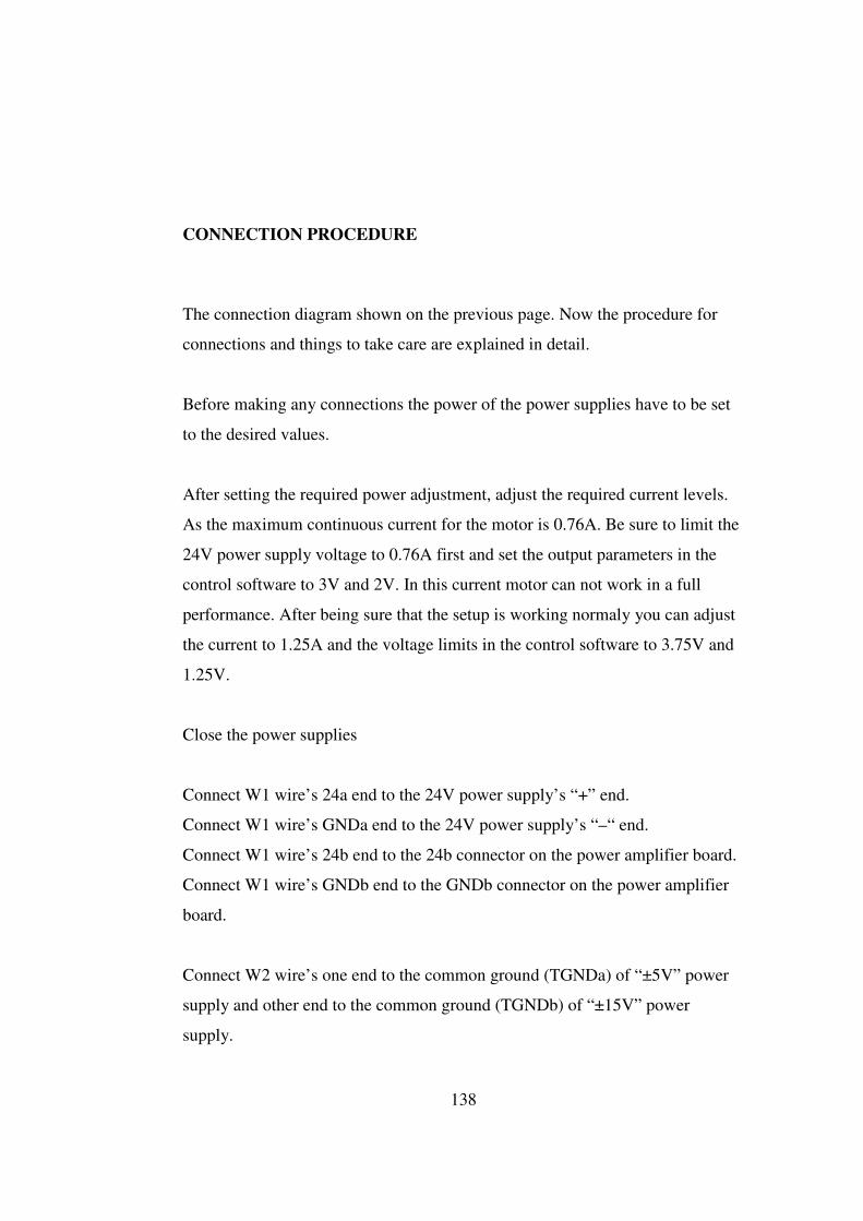
138
CONNECTION PROCEDURE
The connection diagram shown on the previous page. Now the procedure for
connections and things to take care are explained in detail.
Before making any connections the power of the power supplies have to be set
to the desired values.
After setting the required power adjustment, adjust the required current levels.
As the maximum continuous current for the motor is 0.76A. Be sure to limit the
24V power supply voltage to 0.76A first and set the output parameters in the
control software to 3V and 2V. In this current motor can not work in a full
performance. After being sure that the setup is working normaly you can adjust
the current to 1.25A and the voltage limits in the control software to 3.75V and
1.25V.
Close the power supplies
Connect W1 wire’s 24a end to the 24V power supply’s “+” end.
Connect W1 wire’s GNDa end to the 24V power supply’s “–“ end.
Connect W1 wire’s 24b end to the 24b connector on the power amplifier board.
Connect W1 wire’s GNDb end to the GNDb connector on the power amplifier
board.
Connect W2 wire’s one end to the common ground (TGNDa) of “±5V” power
supply and other end to the common ground (TGNDb) of “±15V” power
supply.

139
Connect W3 wire’s -15a end to the “±15 V” power supply’s “-15V” connector.
Connect W3 wire’s +15a end to the “±15 V” power supply’s “+15V” connector.
Connect W3 wire’s -15b end to the “-15 V” on the State Measurement Circuit.
Connect W3 wire’s +15b end to the “+15 V” on the State Measurement Circuit.
Connect W4 TGNDa end to the common ground on the “±5 V” power supply.
Connect W4 +5a end to the “+5V” connector on the “±5 V” power supply.
Connect the socket of the intersection of W4, W6 and W5 to “+5V” on the State
Measurement Circuit. The connector is labeled as “+5V”.
Connect the socket of the intersection of W4, W6 and W10 to TGND on the
State Measurement Circuit. The connector is labeled as TGND.
Connect W6 wire’s -5a end to the “-5V” connector on the “±5 V” power supply.
Connect W6 wire’s posb end to Pos connector’s 1st pin on the State
Measurement Circuit.
Connect W8 wire’s CH_B to the 1st pin of the Enc connector on the State
Masurement Circuit.
Connect W8 wire’s CH_A to the 2nd pin of the Enc connector on the State
Masurement Circuit.
Connect W8 wire’s CH_I to the 3rd pin of the Enc connector on the State
Masurement Circuit.
Connect W12 between connection 57 and connection 60 of the Adapter
Connect W9 wire’s Cmda end to the connection 58 of the Adapter
Connect W9 wire’s Cmdb end to the 1st pin of the Cont connector on the Power
Amplifier Board.

140
Connect W9 wire’s Cga end to the W12 wire.
Connect W9 wire’s Cgb end to the 4th pin of the Cont connector on the Power
Amplifier Board.
Connect W10 wire’s TGNDb end to the W12 wire.
Connect W10 wire’s angb end to the connection 67 of the Adapter.
Connect W10 wire’s posd end to the connection 34 of the Adapter.
Connect W10 wire’s anga end to the Ang connector on the State Measurement
Circuit.
Connect W10 wire’s posc end to the 3rd pin of the Pos connector on the State
Measurement Circuit.
Connect W10 wire’s tgnd end to the TGND on the State Measurement Circuit.
Connect W11 between two A points on the State Measurement Circuit.
Connect W7 wire’s drva1 end to the drva1 connector on the power amplifier
board.
Connect W7 wire’s drva2 end to the drva2 connector on the power amplifier
board.
Connect W7 wire’s drvb2 end to the black wire of the motor.
Do not connect the drvb1 connection of W7 yet. Be sure that drvb1 and drvb2
do not touch each other also.
Power on the computer
Reset the control program and start the program. This action applies “2.5V”
(zero command as control signal.)
Open power “±5V” power supply,

141
Open “±15V” power supply,
Open “24V” power supply, seperately.
Measure the voltage between drva1 and drva2. Set this voltage to “±10mV”
from the power supply coarse voltage adjustment.
Connect W7 wire’s drvb1 end to the red wire of the motor.
Now the controller can be started.