CCC 2013 1

Control and Robustness for QuantumLinear Systems

Control and Robustness for QuantumLinear Systems

Ian R. Petersen †

† School of Engineering and Information Technology, UNSW Canberra

CCC 2013 2

IntroductionIntroduction� Developments in quantum technology and quantum information

provide an important motivation for research in the area of quantumfeedback control systems.

A linear quantum optics experiment at UNSW Canberra Photocourtesy of Elanor Huntington.

CCC 2013 3

� The most recent Nobel prize for Physics was awarded for work inexperimental (open loop) quantum control:Serge Haroche and David J. Wineland”for ground-breaking experimental methods that enable measuringand manipulation of individual quantum systems”

� The stage will soon be reached where the development of quantumtechnologies will require advances in engineering rather thanphysics and quantum control theory is expected to play an importantrole here.

� Quantum physics places fundamental limits on accuracy inestimation and control. These will be the dominant issues inquantum technology.

� New control theories will be needed to deal with models of systemsdescribed by the laws of quantum physics rather than classicalphysics.

CCC 2013 4

� Feedback control of quantum optical systems has potentialapplications in areas such as quantum communications, quantumteleportation, quantum computing, quantum error correction andgravity wave detection.

� Feedback control of quantum systems aims to achieve closed loopproperties such as stability, robustness and entanglement.

� We consider models of quantum systems as quantum stochasticdifferential equations (QSDEs)

� These stochastic models can be used to describe quantum opticaldevices such as optical cavities, linear quantum amplifiers, and finitebandwidth squeezers.

CCC 2013 5

� Recent papers on the feedback control of linear quantum systemshave considered the case in which the feedback controller itself isalso a quantum system. Such feedback control is often referred toas coherent quantum control.

Quantum System

Coherent Quantum Controller

Coherent quantum feedback control.

CCC 2013 6

� One motivation for considering such coherent quantum controlproblems is that coherent controllers have the potential to achieveimproved performance since quantum measurements inherentlyinvolve the destruction of quantum information.

� Also, coherent optical controllers may be much more practical toimplement than measurement feedback based controllers.

� In a paper (James, Nurdin, Petersen, 2008), the coherent quantumH∞ control problem was addressed.

� This paper obtained a solution to this problem in terms of a pair ofalgebraic Riccati equations.

� Also, in a paper (Nurdin, James, Petersen, 2009) the coherentquantum LQG problem was addressed.

� An example of a coherent quantum H∞ system considered in(Nurdin, James, Petersen, 2008), (Maalouf Petersen 2011) isdescribed by the following diagram:

CCC 2013 7

controller

plant

PhaseShift

PSfr

u

y

w

a

v

z

k1 k2

k3

kc1kc2

180◦

acwc0

CCC 2013 8

� The coherent quantum H∞ control approach of James Nurdin andPetersen (2008) was subsequently implemented experimentally byHideo Mabuchi of Stanford University:

CCC 2013 9

� We formulate quantum system models in the Heisenberg Picture ofquantum mechanics which describes the time evolution of operatorsrepresenting system variables such as position and momentum.

� This is as opposed to the Schrodinger picture which describesquantum systems in terms of the time evolution of the quantumstate.

Werner Heisenberg

CCC 2013 10

Linear Quantum System ModelsLinear Quantum System Models

� We formulate a class of linear quantum system models described byquantum stochastic differential equations (QSDEs) derived from thequantum harmonic oscillator (an infinite level quantum system).

� We begin by considering a collection of n independent quantumharmonic oscillators which are defined on a Hilbert space H.

� Corresponding to this is a vector of annihilation operators a:

a =

a1

a2

...an

.

� Each annihilation operator ai is an unbounded linear operator on H.

CCC 2013 11

� The adjoint of the operator ai is denoted a∗i and is referred to as a

creation operator. We use a# to denote the vector of a∗i s:

a# =

a∗1

a∗2...

a∗n

.

� Physically, these operators correspond to the annihilation andcreation of a photon respectively.

� Also, we use the notation aT =[

a1 a2 . . . an

]

, and

a† =(

a#)T

=[

a∗1 a∗

2 . . . a∗n

]

.

CCC 2013 12

Canonical Commutation RelationsCanonical Commutation Relations

� The operators ai and a∗i are such that the following canonical

commutation relations are satisfied

[ai, a∗j ] := aia

∗j − a∗

jai = δij

where δij denotes the Kronecker delta multiplied by the identityoperator on the Hilbert space H.

� We also have the commutation relations

[ai, aj ] = 0, [a∗i , a

∗j ] = 0.

� These relations encapsulate Heisenberg’s uncertainty relation.

CCC 2013 13

� Using the above operator vector notation, the commutation relationscan be written as[

[

aa#

]

,

[

aa#

]†]

=

[

aa#

] [

aa#

]†−(

[

aa#

]# [aa#

]T)T

= Θ

where Θ =

[

I 00 −I

]

is the commutation matrix.

CCC 2013 14

Quantum Wiener ProcessesQuantum Wiener Processes

� The quantum harmonic oscillators described above are assumed tobe coupled to m external independent quantum fields modeled by avector of bosonic annihilation field operators A(t).

� For each annihilation field operator Aj(t), there is a correspondingcreation field operator A∗

j (t).

� These quantum fields may be electromagnetic fields such as a lightbeam produced by a laser.

CCC 2013 15

Hamiltonian, Coupling and Scattering OperatorsHamiltonian, Coupling and Scattering Operators

� In order to describe the joint evolution of the quantum harmonicoscillators and quantum fields, we first specify the Hamiltonianoperator for the quantum system which is a self adjoint operator onH of the form

H =1

2

[

a† aT]

M

[

aa#

]

where M ∈ C2n×2n is a Hermitian matrix of the form

M =

[

M1 M2

M#2 M#

1

]

and M1 = M†1 , M2 = MT

2 .

� Here, M† denotes the complex conjugate transpose of the complexmatrix M , MT denotes the transpose of the complex matrix M ,and M# denotes the complex conjugate of the complex matrix M .

CCC 2013 16

� Also, we specify the coupling operator for the quantum system to bea vector of operators of the form

L =[

N1 N2

]

[

aa#

]

where N1 ∈ Cm×n and N2 ∈ C

m×n. This describes theinteraction between the quantum fields and the quantum system.

� Also, we write[

LL#

]

= N

[

aa#

]

=

[

N1 N2

N#2 N#

1

] [

aa#

]

.

� In addition, we define a scattering matrix which is a unitary matrixS ∈ C

m×m. This describes the interactions between the differentquantum fields.

CCC 2013 17

Quantum Stochastic Differential EquationsQuantum Stochastic Differential Equations

� The quantities (S,L,H) define the joint evolution of the quantumharmonic oscillators and the quantum fields.

� A set of QSDEs describing the quantum system can be obtained.

� The QSDEs for the linear quantum system can be written as[

da(t)da(t)#

]

= F

[

a(t)a(t)#

]

dt + G

[

dA(t)dA(t)#

]

;

[

dAout(t)dAout(t)#

]

= H

[

a(t)a(t)#

]

dt + K

[

dA(t)dA(t)#

]

.

� In many ways these systems behave like classical (complex) linearstochastic systems except that the variables ai(t) and a∗

i (t) arenon-commutative.

� Also, there are restrictions on the structure of the matricesF,G,H,K (physical realizability).

CCC 2013 18

� We can derive the following formulas for the matrices in the QSDEmodel, in terms of the Hamiltonian and coupling matrices.

F = −iΘM − 1

2ΘN †JN ;

G = −ΘN †[

S 00 −S#

]

;

H = N ;

K =

[

S 00 S#

]

.

� Here

J =

[

I 00 −I

]

.

CCC 2013 19

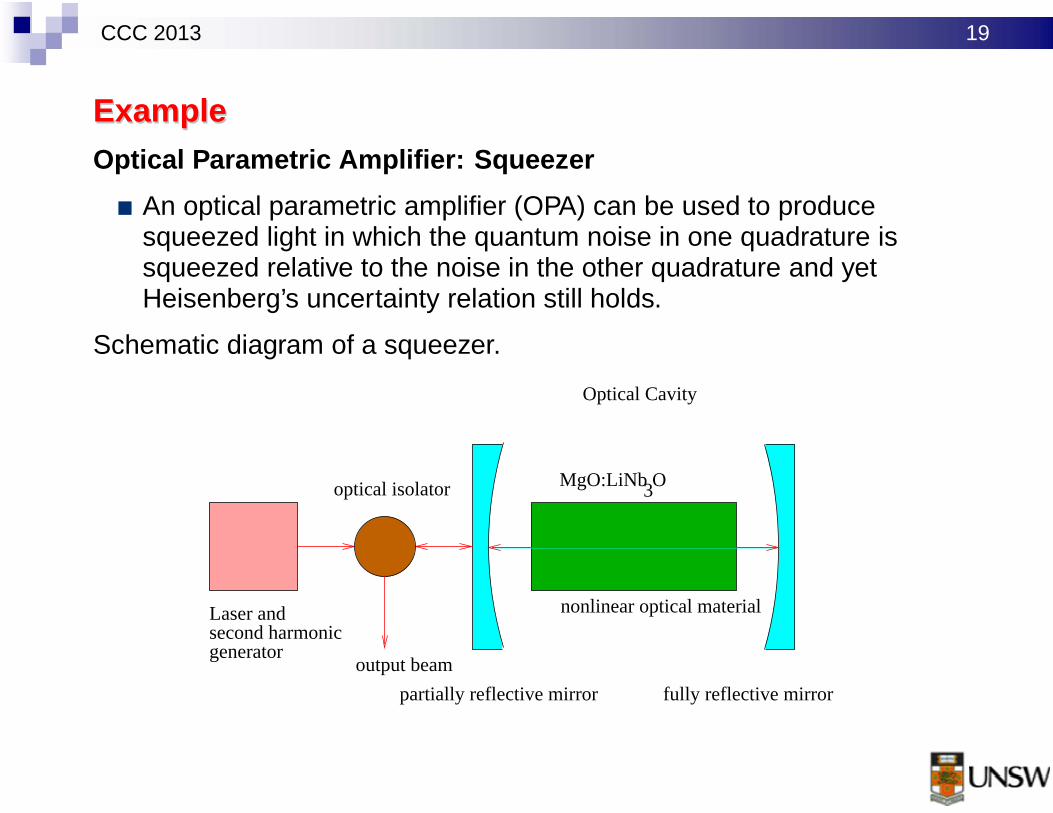
ExampleExampleOptical Parametric Amplifier: Squeezer

� An optical parametric amplifier (OPA) can be used to producesqueezed light in which the quantum noise in one quadrature issqueezed relative to the noise in the other quadrature and yetHeisenberg’s uncertainty relation still holds.

Schematic diagram of a squeezer.

3MgO:LiNb O

nonlinear optical materialsecond harmonicgenerator

output beam

partially reflective mirror fully reflective mirror

Laser and

optical isolator

Optical Cavity

CCC 2013 20

� A simplified model of such a squeezer has (S,L,H) parameters

� S = I ;

� L =√

2κa;

� H = i2χ(

a2 − a†2)

.

� Here κ is a parameter depending on the reflectivity of the partiallyreflecting mirror and χ is a complex parameter depending on thestrength of the nonlinear optical material.

� Using the above formulas, this leads to an approximate linearizedQSDE model of a squeezer as follows:

da = − (κa + χa∗) dt +√

2κdA;

da∗ = − (κa∗ + χ∗a) dt +√

2κdA∗.

� This model is a QSDE quantum linear system model of the formconsidered above.

CCC 2013 21

Physical RealizabilityPhysical Realizability

� Not all QSDEs of the form considered above correspond to physicalquantum systems which satisfy all of the laws of quantummechanics.

� For physical systems, the laws of quantum mechanics require thatthe commutation relations be satisfied for all times.

� This motivates a notion of physical realizability.

� This notion is of particular importance in the problem of coherentquantum feedback control in which the controller itself is a quantumsystem.

� In this case, if a controller is synthesized using a method such asquantum H∞ control or quantum LQG control, it important that thecontroller can be implemented as a physical quantum system.

CCC 2013 22

Definition. QSDEs of the form considered above are physically real-izable if there exist suitably structured complex matrices Θ = Θ†,M = M†, N , S such that S†S = I , and

F = −iΘM − 1

2ΘN †JN ; G = −ΘN †

[

S 00 −S#

]

;

H = N ; K =

[

S 00 S#

]

;

� The conditions in the above definition require that the QSDEscorrespond to a collection of quantum harmonic oscillators withdynamics defined by the operators

(

S,L = N

[

aa#

]

,H =1

2

[

a† aT]

M

[

aa#

])

.

CCC 2013 23

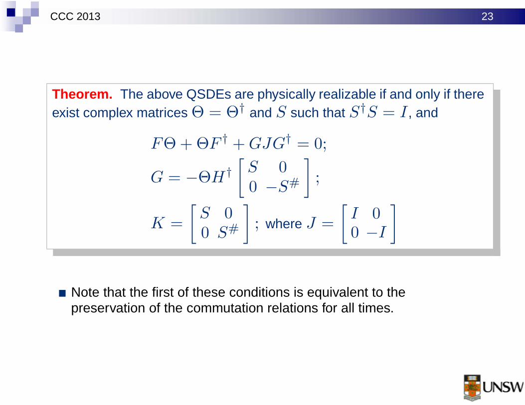
Theorem. The above QSDEs are physically realizable if and only if thereexist complex matrices Θ = Θ† and S such that S†S = I , and

FΘ + ΘF † + GJG† = 0;

G = −ΘH†[

S 00 −S#

]

;

K =

[

S 00 S#

]

; where J =

[

I 00 −I

]

� Note that the first of these conditions is equivalent to thepreservation of the commutation relations for all times.

CCC 2013 24

� We can also characterize physical realizability in terms of the

transfer function matrix Γ(s) = H (sI − F )−1

G + K of a linearquantum system.

Theorem. (See Shaiju and Petersen, 2012) The linear quantum systemdefined by the above QSDEs is physically realizable if and only if thesystem transfer function matrix Γ(s) satisfies

Γ(−s∗)†JΓ(s) = J

(i.e., the system is (J, J)-unitary) and the matrix K is of the form K =[

S 00 S#

]

where S†S = I .

CCC 2013 25

RecapRecap

� Coherent feedback controllers for linear quantum systems can besynthesized in a variety of ways to ensure that the controller isphysically realizable.

� These include quantum H∞ control

M. R. James, H. I. Nurdin, and I. R. Petersen, “H∞ control of linearquantum stochastic systems,” IEEE Transactions on Automatic Control,vol. 53, no. 8, pp. 1787–1803, 2008.

� Another approach is quantum LQG control

H. I. Nurdin, M. R. James, and I. R. Petersen, “Coherent quantum LQGcontrol,” Automatica, vol. 45, no. 8, pp. 1837–1846, 2009.

� However, so far this quantum LQG problem has only been solved bybrute force optimization methods and there do not as yet generalmethods to solve large scale quantum LQG control problems.

CCC 2013 26

ExampleExample

� We consider a problem of stabilization via coherent feedback control.

� In this example, an unstable linear quantum optical system is to becontrolled via a coherent quantum feedback controller in which thecontroller itself is a quantum system. This requires that the controlleris physically realizable.

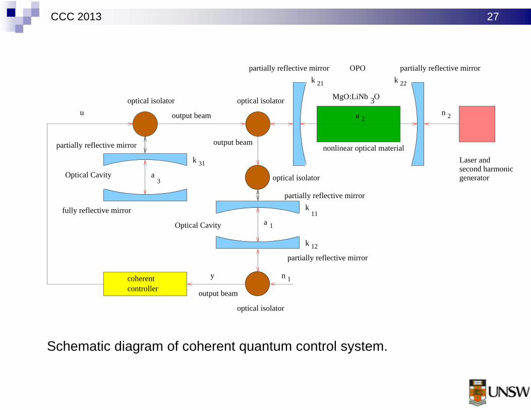
� The quantum system to be controlled consists of the cascadeconnection of an optical parametric oscillator (OPO) and two opticalcavities.

CCC 2013 27

n

22

31

11

12

1

1

nonlinear optical material

Optical Cavity

2

partially reflective mirror

3MgO:LiNb Ooptical isolator

second harmonicgenerator

Laser and

partially reflective mirror partially reflective mirrorOPO

fully reflective mirror

Optical Cavity

partially reflective mirror

partially reflective mirror

optical isolator

optical isolator

output beam

output beam

coherentcontroller

k

k

k

k k

a

a

y

u

output beam

optical isolator

n

3

21

a 2

Schematic diagram of coherent quantum control system.

CCC 2013 28

� The following linear quantum system model is constructed for thequantum plant.

da1(t)da1(t)

∗

da2(t)da2(t)

∗

da3(t)da3(t)

∗

= F

a1(t)a1(t)

∗

a2(t)a2(t)

∗

a3(t)a3(t)

∗

dt + G

[

du(t)du(t)∗

]

+ D

dn1(t)dn1(t)

∗

dn2(t)dn2(t)

∗

;

[

dy(t)dy(t)∗

]

= H

a1(t)a1(t)

∗

a2(t)a2(t)

∗

a3(t)a3(t)

∗

dt + K

dn1(t)dn1(t)

∗

dn2(t)dn2(t)

∗

.

CCC 2013 29

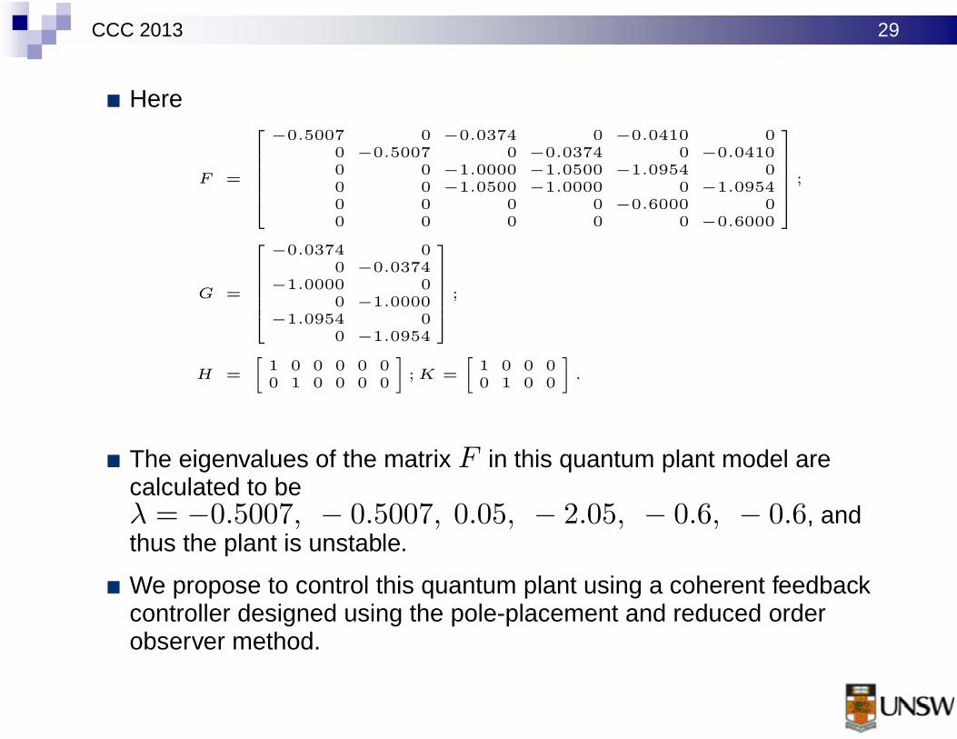
� Here

F =

2

6

6

6

6

6

4

−0.5007 0 −0.0374 0 −0.0410 0

0 −0.5007 0 −0.0374 0 −0.0410

0 0 −1.0000 −1.0500 −1.0954 0

0 0 −1.0500 −1.0000 0 −1.0954

0 0 0 0 −0.6000 0

0 0 0 0 0 −0.6000

3

7

7

7

7

7

5

;

G =

2

6

6

6

6

6

4

−0.0374 0

0 −0.0374

−1.0000 0

0 −1.0000

−1.0954 0

0 −1.0954

3

7

7

7

7

7

5

;

H =

»

1 0 0 0 0 0

0 1 0 0 0 0

–

; K =

»

1 0 0 0

0 1 0 0

–

.

� The eigenvalues of the matrix F in this quantum plant model arecalculated to beλ = −0.5007, − 0.5007, 0.05, − 2.05, − 0.6, − 0.6, andthus the plant is unstable.

� We propose to control this quantum plant using a coherent feedbackcontroller designed using the pole-placement and reduced orderobserver method.

CCC 2013 30

� The reduced order observer based controller is defined as follows:

dz = Fczdt + Gc

[

dydy∗

]

;

[

dudu∗

]

= Hczdt + Kc

[

dydy∗

]

where

Fc = F22 − HoF12 − (G2 − H0G1)K2;

Gc = F21 + F22Ho − HoF12Ho − HoF11

+(G2 − HoG1) (K1 + K2Ho) ;

Hc = K2; Kc = K1 + K2Ho.

CCC 2013 31

� The observer gain matrix Ho is chosen as

Ho = 103 ×

1.5928 3.72293.7229 1.5928

−1.9274 −3.3729−3.3729 −1.9274

,

which leads to observer poles λ = −11, − 11, − 10, − 10.

� Also, the state feedback controller matrix is chosen as

Ksf =

[

1.2376 −0.0008 0.0201 0.0043 0.0238 0.0007−0.0008 1.2376 0.0043 0.0201 0.0007 0.0238

]

,

which leads to the state feedback closed loop poles λ =−2.1498, −0.9618, −0.6882, −0.0882±0.0368ı, −0.4102.

CCC 2013 32

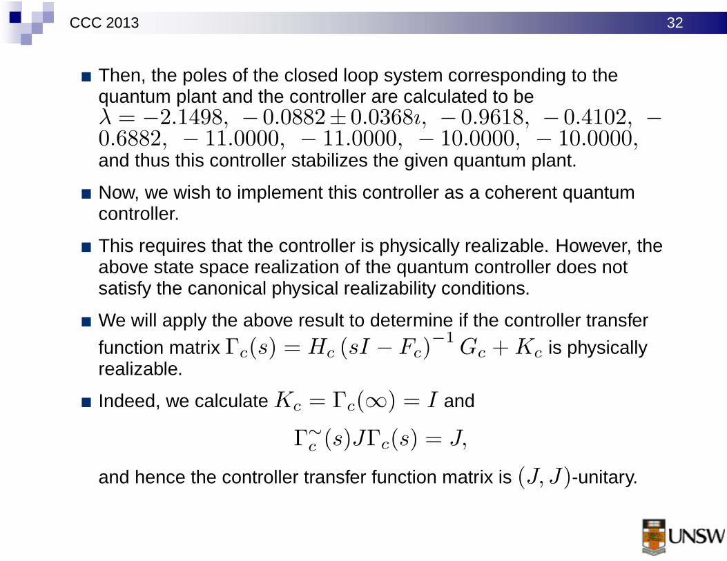
� Then, the poles of the closed loop system corresponding to thequantum plant and the controller are calculated to beλ = −2.1498, − 0.0882± 0.0368ı, − 0.9618, − 0.4102, −0.6882, − 11.0000, − 11.0000, − 10.0000, − 10.0000,and thus this controller stabilizes the given quantum plant.

� Now, we wish to implement this controller as a coherent quantumcontroller.

� This requires that the controller is physically realizable. However, theabove state space realization of the quantum controller does notsatisfy the canonical physical realizability conditions.

� We will apply the above result to determine if the controller transfer

function matrix Γc(s) = Hc (sI − Fc)−1

Gc + Kc is physicallyrealizable.

� Indeed, we calculate Kc = Γc(∞) = I and

Γ∼c (s)JΓc(s) = J,

and hence the controller transfer function matrix is (J, J)-unitary.

CCC 2013 33

� Also, the poles of the controller transfer function matrix arecalculated to be at s = −10.5301 ± 1.3545ı ands = −10.5251 ± 1.3385ı.

� Hence, it follows that the conditions of the theorem are satisfied andtherefore, the controller transfer function matrix Γc(s) is physicallyrealizable and can be implemented as a quantum system.

� We can implement the controller transfer function as ininterconnection of optical devices using the algorithm in

H. Nurdin, “Synthesis of linear quantum stochastic systems via quantumfeedback networks,” IEEE Transactions on Automatic Control, vol. 55,no. 4, pp. 1008 –1013, April 2010.

CCC 2013 34

Robust Stability of Nonlinear Quantum SystemsRobust Stability of Nonlinear Quantum Systems

� Most interesting quantum phenomena such as entanglement andsqueezing for continuous variable (infinite level) quantum systemsoccur when we have a nonlinear quantum system rather than alinear one.

� We would like to extend our existing linear quantum systems theoryto the nonlinear case.

� Also, the issue of robustness to nonlinear perturbations in thedynamics is important in any linear feedback control system.

� We now consider the problem of robust stability for a quantumsystem defined in terms of a triple (S,L,H) in which the quantumsystem Hamiltonian is decomposed as H = H1 + H2 where H1is a known nominal (quadratic) Hamiltonian and H2 is aperturbation (non-quadratic) Hamiltonian, which is contained in aspecified set of Hamiltonians W .

CCC 2013 35

� Our solution to this problem is a quantum version of the small gaintheorem for quantum systems which are nominally linear but aresubject to sector bounded nonlinearities.

� This result can be applied to the stability analysis of perturbedquantum linear systems.

� Alternatively, it can be applied to closed loop quantum systemsobtained when we apply a coherent quantum H∞ controller to alinear quantum system subject to nonlinear sector boundedperturbations.

CCC 2013 36

� Consider an open quantum system defined by parameters(S,L,H) where H = H1 + H2.

� We letH2 = f(ζ, ζ∗)

� Here ζ is a scalar operator on the underlying Hilbert space.

CCC 2013 37

� Also, we consider the sector bound condition

∂f(ζ, ζ∗)

∂ζ

∗ ∂f(ζ, ζ∗)

∂ζ≤ 1

γ2ζζ∗ + δ1

and the smoothness condition

∂2f(ζ, ζ∗)

∂ζ2

∗∂2f(ζ, ζ∗)

∂ζ2≤ δ2.

CCC 2013 38

� Representation of the sector bound condition:

∂f(ζ,ζ∗)∂ζ

ζ

CCC 2013 39

� Then we define the set of allowable perturbations W as follows:

Definition.

W =

H2 = f(ζ, ζ∗) such that∂f(ζ,ζ∗)

∂ζ

∗ ∂f(ζ,ζ∗)∂ζ

≤ 1γ2 ζζ∗ + δ1 and

∂2f(ζ,ζ∗)∂ζ2

∂2f(ζ,ζ∗)∂ζ2

∗≤ δ2

.

CCC 2013 40

� Also as previously in the case of linear quantum systems, H1 is ofthe form

H1 =1

2

[

a† aT]

M

[

aa#

]

where M ∈ C2n×2n is a Hermitian matrix of the form

M =

[

M1 M2

M#2 M#

1

]

and M1 = M†1 , M2 = MT

2 .

� In addition, we assume L is of the form

L =[

N1 N2

]

[

aa#

]

where N1 ∈ Cm×n and N2 ∈ C

m×n. Also, S = I .

CCC 2013 41

Definition. An uncertain open quantum system defined by (S,L,H)where H = H1 + H2 with quadratic H1 as above, H2 ∈ W , andlinear L as above, is said to be robustly mean square stable if thereexist constants c1 > 0, c2 > 0 and c3 ≥ 0 such that for any H2 ∈ W ,

⟨

[

a(t)a(t)#

]† [a(t)

a(t)#

]

⟩

≤ c1e−c2t

⟨

[

aa#

]† [a

a#

]

⟩

+ c3 ∀t ≥ 0.

CCC 2013 42

� We define

ζ = E1a + E2a#

=[

E1 E2

]

[

aa#

]

= E

[

aa#

]

where ζ is assumed to be a scalar operator.

� The following frequency domain small gain condition provides asufficient condition for robust mean square stability when H2 ∈ W :

CCC 2013 43

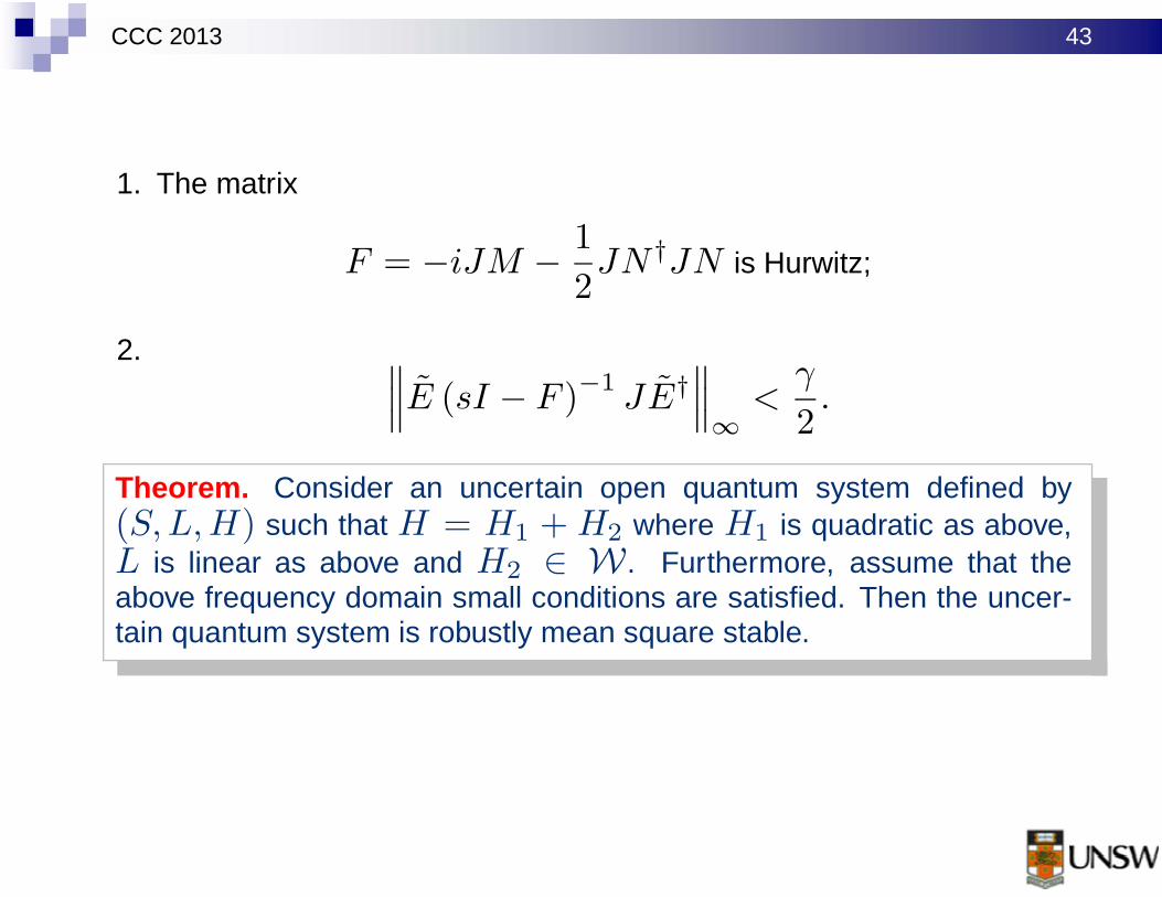
1. The matrix

F = −iJM − 1

2JN †JN is Hurwitz;

2.∥

∥

∥E (sI − F )

−1JE†

∥

∥

∥

∞<

γ

2.

Theorem. Consider an uncertain open quantum system defined by(S,L,H) such that H = H1 + H2 where H1 is quadratic as above,L is linear as above and H2 ∈ W . Furthermore, assume that theabove frequency domain small conditions are satisfied. Then the uncer-tain quantum system is robustly mean square stable.

CCC 2013 44

A Josephson Junction in a Resonant Cavity SystemA Josephson Junction in a Resonant Cavity System� A Josephson junction consists of a thin insulating material between

two superconducting layers as illustrated below:

SuperconductorSuperconductor I

Electromagnetic Resonant Cavity

Insulator

CCC 2013 45

� The following Hamiltonian can be obtained for this quantum system

H =1

2

[

a† aT]

M

[

aa#

]

− µ cos(a2 + a∗

2√2

)

where a =

[

a1

a2

]

, M is a Hermitian matrix and µ > 0.

� This leads to the perturbation Hamiltonian

H2 = f(ζ, ζ∗) = −µ cos(ζ + ζ∗√

2)

where ζ = a2.

� The derivative of a cosine function is a sine function which is sectorbounded with γ = µ√

2.

CCC 2013 46

� We assume that the cavity and Josephson modes are coupled tofields corresponding to coupling operators of the form

L =

[√κ1a1√κ2a2

]

.

� We choose physically reasonable values for the parameters in thissystem except for the parameter κ2 which we allow to vary.

� For various values of κ2 we form the transfer function

Gκ2(s) = E (sI − F )

−1JE† and calculate its H∞ norm.

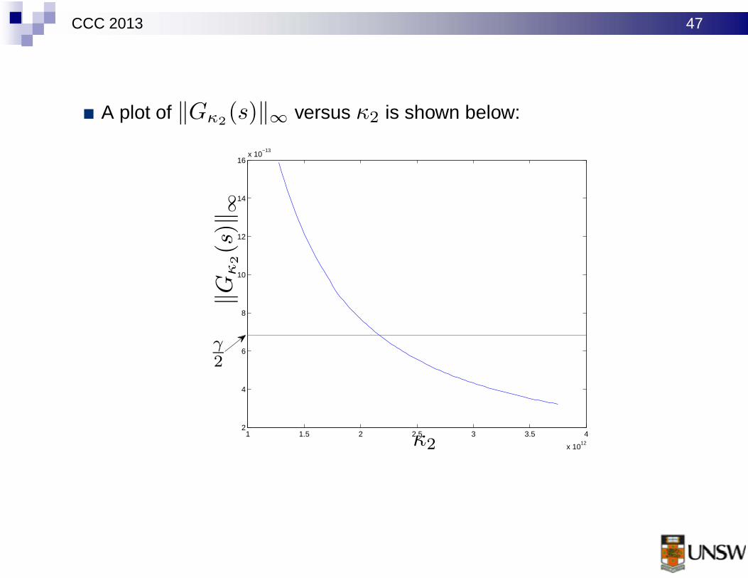
CCC 2013 47

� A plot of ‖Gκ2(s)‖∞ versus κ2 is shown below:

1 1.5 2 2.5 3 3.5 4

x 1012

2

4

6

8

10

12

14

16x 10

−13

‖Gκ2(s

)‖∞

κ2

γ2

CCC 2013 48

� From this plot we can see that stability can be guaranteed forκ2 > 2.2 × 1012.

� Hence, choosing a value of κ2 = 2.5× 1012, it follows that stabilityof Josephson junction system can be guaranteed.

� Indeed, with this value of κ2, we calculate the matrixF = −iJM − 1

2JN †JN and find its eigenvalues to be

−5.0000 × 1010 ± 3.3507 × 103i and−1.2500 × 1012 ± 1.4842 × 103i which implies that the matrixF is Hurwitz.

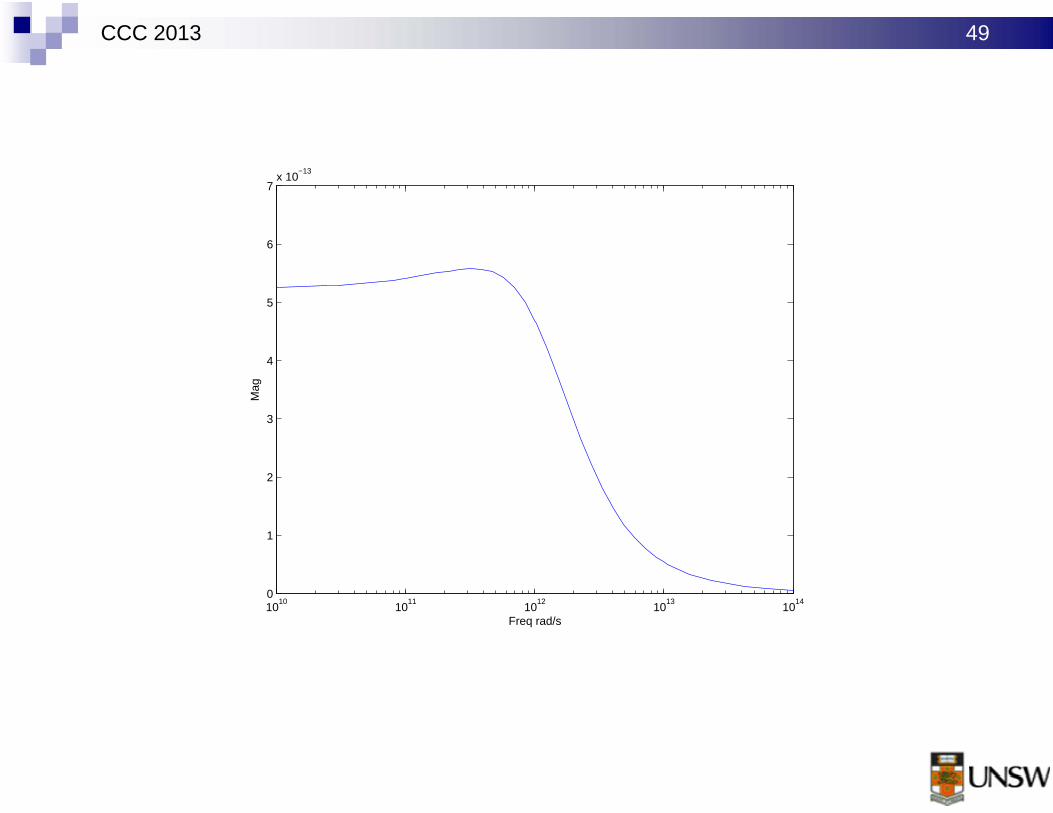
� Also, a magnitude Bode plot of the corresponding transfer functionGκ2

(s) is shown below which implies that‖Gκ1,κ2

(s)‖∞ = 5.5554 × 10−13 < γ/2 = 6.8209 × 10−13

and hence, we conclude that the quantum system is robustly meansquare stable.

CCC 2013 49

1010

1011

1012

1013

1014

0

1

2

3

4

5

6

7x 10

−13

Freq rad/s

Mag

CCC 2013 50

ConclusionsConclusions

� The control of linear quantum systems is an emerging field withimportant applications in quantum optics.

� The theory of linear quantum systems has close connections tostandard linear systems theory but with the important distinction thatthe variables of interest are non-commutative.

� Central to the theory of quantum linear systems is the notion ofphysical realizability which characterizes when a linear systemmodel is really quantum.

� It is also possible to extend the theory to allow for nonlinear quantumsystems using classical ideas from robust control theory.

� The study of nonlinear quantum systems is needed to capture trulyquantum phenomenon such as entanglement, squeezing andquantum superpositions.

CCC 2013 51

� We are also extending our theory to the theory of finite levelquantum systems (e.g. atoms) interacting with quantum fields:

L. A. D. Espinosa, Z. Miao, I. R. Petersen, V. Ugrinovskii, and M. R.James, “On the preservation of commutation and anticommutationrelations of n-level quantum systems,” in Proceedings of the 2013American Control Conference, Washington, DC, June 2013.

� In this case, the QSDEs are bilinear systems rather than linearsystems.

� All of these areas are rich with theoretical challenges which seemvery ameniable to the tools of control theory.