Contributions to Theory of Few and Many-Body

Systems in Lower Dimensions

Tianhao Ren

Submitted in partial fulfillment of therequirements for the degree of

Doctor of Philosophyin the Graduate School of Arts and Sciences

COLUMBIA UNIVERSITY

2019

c© 2019

Tianhao Ren

All rights reserved

Abstract

Contributions to Theory of Few and Many-Body Systems in Lower Dimensions

Tianhao Ren

Few and many-body systems usually feature interesting and novel behaviors com-

pared with their counterparts in three dimensions. On one hand, low dimensional

physics presents challenges due to strong interactions and divergences in the pertur-

bation theory; On the other hand, there exist powerful theoretical tools such as the

renormalization group and the Bethe ansatz. In this thesis, I discuss two examples:

three interacting bosons in two dimensions and interacting bosons/fermions in one

dimension. In both examples, there are intraspecies repulsion as well as interspecies

attraction, producing a rich spectrum of phenomena. In the former example, a univer-

sal curve of three-body binding energies versus scattering lengths is obtained efficiently

by evolving a matrix renormalization group equation. In the latter example, exact so-

lutions for the BCS-BEC crossover are obtained and the unexpected robust features in

their excitation spectra are explained by a comprehensive semiclassical analysis.

Contents

Acknowledgments iii

Dedication iv

Chapter 1 Introduction 1

Chapter 2 Three-Boson Bound States in Two Dimensions 4

2.1 Introduction . . . . . . . . . . . . . . . . . . . . . . . . . . . . . . . . . . . . . . . . . . 4

2.2 Formalism . . . . . . . . . . . . . . . . . . . . . . . . . . . . . . . . . . . . . . . . . . . 7

2.2.1 Parameterization of the Configuration Space . . . . . . . . . . . . . . . . . . . 7

2.2.2 Solution of the One-Dimensional Schrodinger Equation . . . . . . . . . . . . . . 11

2.2.3 Running Basis . . . . . . . . . . . . . . . . . . . . . . . . . . . . . . . . . . . . 14

2.3 Eigenstates and Eigenvalue of Operator U(r) . . . . . . . . . . . . . . . . . . . . . . . 16

2.3.1 Zero Angular Momentum: Analytics . . . . . . . . . . . . . . . . . . . . . . . . 17

2.3.2 Zero Angular Momentum: Numerics . . . . . . . . . . . . . . . . . . . . . . . . 22

2.3.3 Non-Zero Angular Momentum . . . . . . . . . . . . . . . . . . . . . . . . . . . 24

2.4 Conclusion . . . . . . . . . . . . . . . . . . . . . . . . . . . . . . . . . . . . . . . . . . 28

Chapter 3 Exact Solutions to Two-Component Many-Body Systems in One Di-

mension 30

3.1 Introduction . . . . . . . . . . . . . . . . . . . . . . . . . . . . . . . . . . . . . . . . . . 30

3.2 Models and Their Integrability . . . . . . . . . . . . . . . . . . . . . . . . . . . . . . . 32

3.2.1 Models . . . . . . . . . . . . . . . . . . . . . . . . . . . . . . . . . . . . . . . . 32

3.2.2 Integrability . . . . . . . . . . . . . . . . . . . . . . . . . . . . . . . . . . . . . . 35

3.3 Uniform Regime with c1 > c2 > 0 . . . . . . . . . . . . . . . . . . . . . . . . . . . . . . 43

3.3.1 Level Condensation and Limiting Fermi Momentum Q∗ . . . . . . . . . . . . . 44

3.3.2 BCS-BEC Crossover without External Magnetic Field . . . . . . . . . . . . . . 50

3.3.3 Phase Diagram in Presence of External Magnetic Field . . . . . . . . . . . . . 60

i

3.4 Bright Solitons with c1 < c2 . . . . . . . . . . . . . . . . . . . . . . . . . . . . . . . . . 64

3.5 Conclusion . . . . . . . . . . . . . . . . . . . . . . . . . . . . . . . . . . . . . . . . . . 67

Chapter 4 Solitons in One Dimensional Systems at BCS-BEC Crossover 69

4.1 Introduction . . . . . . . . . . . . . . . . . . . . . . . . . . . . . . . . . . . . . . . . . . 69

4.2 Review of Exact Solutions and their Relation to Solitons . . . . . . . . . . . . . . . . . 70

4.3 General Formalism . . . . . . . . . . . . . . . . . . . . . . . . . . . . . . . . . . . . . . 74

4.3.1 Dark Soliton . . . . . . . . . . . . . . . . . . . . . . . . . . . . . . . . . . . . . 76

4.3.2 Grey Soliton . . . . . . . . . . . . . . . . . . . . . . . . . . . . . . . . . . . . . 80

4.4 Theory of S = 1/2 Soliton . . . . . . . . . . . . . . . . . . . . . . . . . . . . . . . . . . 84

4.4.1 Deep BCS Side . . . . . . . . . . . . . . . . . . . . . . . . . . . . . . . . . . . . 84

4.4.2 Deep BEC Side . . . . . . . . . . . . . . . . . . . . . . . . . . . . . . . . . . . . 88

4.5 Theory of S = 0 Soliton . . . . . . . . . . . . . . . . . . . . . . . . . . . . . . . . . . . 91

4.5.1 Deep BEC Side . . . . . . . . . . . . . . . . . . . . . . . . . . . . . . . . . . . . 92

4.5.2 Deep BCS Side . . . . . . . . . . . . . . . . . . . . . . . . . . . . . . . . . . . . 92

4.5.3 Crossover Problem . . . . . . . . . . . . . . . . . . . . . . . . . . . . . . . . . . 95

4.6 Conclusion . . . . . . . . . . . . . . . . . . . . . . . . . . . . . . . . . . . . . . . . . . 98

Bibliography 99

Appendix A Calculation of the Matrix Elements of the Berry Connection 108

Appendix B First Order Correction to Adiabatics 110

Appendix C Algebraic Bethe Ansatz for Two-Component Systems 114

ii

Acknowledgments

I gratefully acknowledge the support and guidance of Prof. Igor Aleiner, from whom I learned not

only almost all of my physics, but also the altitudes and methods for doing academic research.

I would like to acknowledge the help from my friends at Columbia, they are always a source of

discussion and support.

I am especially grateful to my parents and my wife, without their support, my journey toward graduate

study would not have been possible.

iii

This work is dedicated to my wife Yuanwen and my son Ruicheng.

iv

Chapter 1

Introduction

Life in lower dimensions is qualitatively different from that in three dimensions. From the few-body

aspect, there is no threshold for attractive interaction to produce a bound state out of two particles.

There is no Efimov effect [27, 26] for three resonantly interacting particles, thus a single quantity such

as the binding energy of the shallow dimer is sufficient for the description of the few-body universality.

From the many-body aspect, thermal fluctuations are enhanced since the reduced dimensionality

makes the integration over the Bogoliubov 1/k2 law logarithmically or linearly divergent. This rules

out spontaneously broken continuous symmetry for systems with short-ranged interactions in lower

dimensions, known as the Hohenberg-Mermin-Wagner theorem [70, 46]. Likewise, perturbation theory

breaks down in lower dimensions, and electronic transport is blocked by random disorder, both are

result of similar divergences. Density wave states are favored in lower dimensions since Fermi surface

nesting is more prominent. Landau theory of Fermi liquids breaks down in lower dimensions since

electronic degree of freedom fractionalizes into charge and spin degrees of freedom with different

velocity of propagation, giving rise to a new universality class of quantum liquid known as Tomonaga-

Luttinger liquid [43]. The novel features of low dimensional physics have attracted a great deal of

research interest and become one of the central topics in condensed matter physics.

Although the theory of few and many-body systems in lower dimensions poses challenges due to

strong interactions and divergences, there are powerful theoretical tools to deal with a number of

interesting model systems. For few-body theory, effective field theory and nonperturbative renormal-

ization have supplemented the conventional approach of directly solving the Schrodinger equation; For

many-body theory, bosonization is developed to describe the universality class of Tomonaga-Luttinger

liquid, Bethe ansatz technique is extensively generalized and applied to a wide range of one dimensional

1

models, and numerical techniques such as quantum Monte-Carlo and density matrix renormalization

group are successfully implemented to give out low energy properties with high accuracy. Nowadays,

theoreticians are equipped with numerous results and tools to explore the world of low dimensional

physics. Also the situation of model systems in lower dimensions as a playground for theoreticians to

test ideas and gain insights has been changed recently, due to experimental realizations of quasi-one

and two dimensional systems in semiconductor quantum well structures, confined cold atom gases and

organic compounds. As a result, the theory of low dimensional systems has gained reignited interest

and been confronted with real-world tests and applications.

In this thesis, we make several contributions to the theory of few and many-body systems in lower

dimensions. In chapter 2 we investigate the few body physics of three interacting bosons in two

dimensions. The bosons are classified in two species, where the interaction between same species is

repulsive and between different species is attractive. Instead of solving variants of the Schrodinger

equation or integral equations for the scattering amplitude, a matrix renormalization group equation

is derived and efficiently evolved to search for possible three-body bound states for the system under

study. Only one trimer is found and its binding energy ε(3)b is determined for a wide range of scattering

lengths. Although there is no universal phenomenon like accumulation of Efimov trimers, a universal

curve of ε(3)b /ε

(2)b (ε

(2)b is the binding energy of the shallow dimer) is found, which depends only on the

scattering lengths but not on the microscopic details of the interactions.

In chapter 3, we introduce a new type of models for two-component systems in one dimension

subject to Bethe ansatz analysis. The intraspecies interaction c1 is repulsive and the interspecies

interaction c2 is attractive, and they are tunable via Feshbach resonances. This type of models

interpolates between the Lieb-Liniger model and the Yang-Gaudin model, and its integrability is

obtained by fine-tuning the resonant energies. There are two interesting regimes of this type of

models, showing different behaviors. In the regime with c1 > c2, the ground state is a Fermi sea of

two-strings, where the Fermi momentum Q is constrained to be smaller than a certain value Q∗, and

it provides an exactly solvable model of BCS-BEC crossover in one dimension. In the other regime

with c1 < c2, the ground state is a single bright soliton even for fermionic atoms, which reveals itself

as an embedded string solution.

In chapter 4, we develop a comprehensive semiclassical theory of solitons in one dimensional

systems at BCS-BEC crossover. The exact solutions in chapter 3 show robust features of the low

energy excitation spectra along the whole crossover, for example, the minimum energy of the S = 1/2

excitation remains exactly at kF = πn/2, where nmF (mF is the mass of the fermionic atom) is

the total mass density of the system. Our semiclassical theory explains them as a result of a special

2

feature of one dimensional systems that the conventional quasiparticle is not stable with respect to

soliton formation, thus their validity is beyond integrability. The proposed semiclassical theory agrees

quantitatively with the exact solutions on both the deep BCS and deep BEC side and describes

qualitatively the smooth crossover. Besides, it resolves the inconsistency of existing semiclassical

theory with the exact solution of soliton-like S = 0 excitations on the deep BCS side by a new

proposal of soliton configuration.

3

Chapter 2

Three-Boson Bound States in Two

Dimensions

2.1 Introduction

The conventional approach to the quantum three-body problem in three dimensions is introduced

by Skorniakov and Ter-Martirosian for three fermions in the zero-range-interaction limit [96]. They

derived an integral equation for the scattering matrix between an atom and a weakly bound dimer

consisting of two atoms via the diagrammatic technique:

T3(k, k′, E) =1

E + i0− k2/m− k′2/m− kk′/m

+2

∫d3p

(2π)3

1

E + i0− k2/m− p2/m− kp/mT2(E − 3p2/4m)T3(p, k′, E),

(2.1)

where T3 and T2 are the T -matrix for atom-dimer and atom-atom scatterings respectively. It was

then recognized by Danilov [17] that the Skorniakov-Ter-Martirosian equation gives a spectrum that

is not bounded from below if applied to the case of three identical bosons. This pathology was then

resolved by Efimov [27, 26]. He showed that in the resonant limit that the two-particle scattering

length a → ±∞, there is a condensation of three-particle bound states at the scattering threshold,

whose binding energies form a discrete series:

ε(3)b (n)→

(e−2π/s0

)n−n∗ ~2κ2∗

m, n→ +∞, (2.2)

4

where the consecutive binding energies have a universal ratio e−2π/s0 ≈ 1/515. This shows that in

addition to the two-body parameter such as the scattering length a, we need to introduce yet another

three-body parameter, which can be taken as the scale κ∗. More surprisingly, there are three-particle

bound states even in the absence of two-particle bound state, which are referred to as the Borromean

halos. These and other related three-body phenomena are collectively referred to as the Efimov

physics, and they can be understood naturally from a renormalization group perspective [9, 45, 5].

In two dimensions, it is now known that there is no Efimov effect in the sense that there is no

condensation of three-particle bound states or any Borromean halo [5]. As a result, there is no need to

introduce any three-body parameter and the binding energy of any possible few-particle bound state is

proportional to the binding energy of the shallow dimer. For example, there are only two three-particle

bound states with binding energies ε(3)b (1) = 16.52ε

(2)b and ε

(3)b (2) = 1.27ε

(2)b for identical bosons with

zero-ranged potential [13, 12]. It is then worthwhile to generalize the scheme to more complicated

systems with possible new universal features. In fact, the universal properties of three-body systems

in two dimensions are readily explored in mass-imbalanced systems [6, 7, 8] and for charged particles

[14, 34]. Furthermore, it is of particular interest to study systems with interspecies attraction as well

as intraspecies repulsion, where few-body bound states plays an important role in determining the

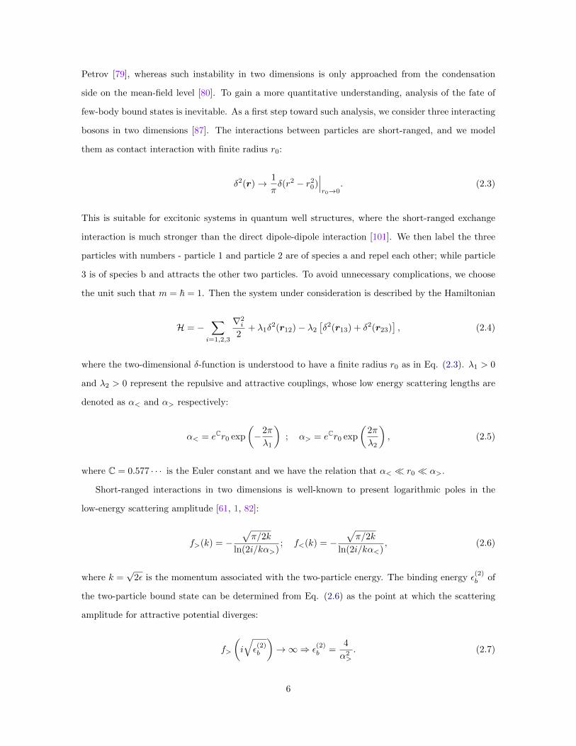
nature of the ground state. A primary example is provided by the exciton Bose-Einstein condensates

in GaAs-based quantum well structures [18, 102, 54, 19], where there are two kinds of bright excitons

with spin projection Jz = ±1 to the structural axis. The same spin projections repel each other and

the opposite spin projections attract each other [72, 73, 15], as shown in Fig (2.1).

Figure 2.1: Excitons in GaAs-based quantum well structures. The excitons with spin projectionJz = ±1 are optically active, thus they are referred to as the bright excitons. The coupling betweenopposite spins is attractive, leading to a shallow dimer, and the coupling between like spins is repulsive.

For these bright excitons in quantum wells, formation of few-body bound states is the possible

route to the instability of the condensates. A similar instability in three dimensions is resolved by

5

Petrov [79], whereas such instability in two dimensions is only approached from the condensation

side on the mean-field level [80]. To gain a more quantitative understanding, analysis of the fate of

few-body bound states is inevitable. As a first step toward such analysis, we consider three interacting

bosons in two dimensions [87]. The interactions between particles are short-ranged, and we model

them as contact interaction with finite radius r0:

δ2(r)→ 1

πδ(r2 − r2

0)∣∣∣r0→0

. (2.3)

This is suitable for excitonic systems in quantum well structures, where the short-ranged exchange

interaction is much stronger than the direct dipole-dipole interaction [101]. We then label the three

particles with numbers - particle 1 and particle 2 are of species a and repel each other; while particle

3 is of species b and attracts the other two particles. To avoid unnecessary complications, we choose

the unit such that m = ~ = 1. Then the system under consideration is described by the Hamiltonian

H = −∑

i=1,2,3

∇2i

2+ λ1δ

2(r12)− λ2

[δ2(r13) + δ2(r23)

], (2.4)

where the two-dimensional δ-function is understood to have a finite radius r0 as in Eq. (2.3). λ1 > 0

and λ2 > 0 represent the repulsive and attractive couplings, whose low energy scattering lengths are

denoted as α< and α> respectively:

α< = eCr0 exp

(−2π

λ1

); α> = eCr0 exp

(2π

λ2

), (2.5)

where C = 0.577 · · · is the Euler constant and we have the relation that α< r0 α>.

Short-ranged interactions in two dimensions is well-known to present logarithmic poles in the

low-energy scattering amplitude [61, 1, 82]:

f>(k) = −√π/2k

ln(2i/kα>); f<(k) = −

√π/2k

ln(2i/kα<), (2.6)

where k =√

2ε is the momentum associated with the two-particle energy. The binding energy ε(2)b of

the two-particle bound state can be determined from Eq. (2.6) as the point at which the scattering

amplitude for attractive potential diverges:

f>

(i

√ε(2)b

)→∞⇒ ε

(2)b =

4

α2>

. (2.7)

6

The corresponding pole for the repulsive potential occurs at momentum |k| 1/r0, which is beyond

the logarithmic pole approximation, and must be disregarded in the calculation as a spurious solution.

In this chapter, we will show that the system under consideration support at most one three-

particle bound state. We will also determine the three-particle bound state energies ε(3)b for a wide

range of scattering lengths α> and α<, which traces out a universal curve of ε(3)b /ε

(2)b with no reference

to microscopic details. This chapter is organized as follows. In Sec. 2.2 we introduce the parameteriza-

tion scheme of the problem, and give the formal solution to the resulting one-dimensional Schrodinger

equation via a boundary-matching-matrix technique. We also introduce a convenient running basis

to the problem, which is suited for numerical implementations. In Sec. 2.3 we give out the explicit

solutions for zero and nonzero angular momenta separately. Large scale behaviors are analyzed analyt-

ically and three-particle binding energies are calculated numerically. Finally in Sec. 2.4 we summarize

the results and compare our methods with existing ones. Some technical details are relegated to the

appendices.

2.2 Formalism

2.2.1 Parameterization of the Configuration Space

For the configuration space of the system under consideration, we use the Faddeev parameterization

with Jacobi coordinates [29] (see Fig. 2.2)

r12 = r1 − r2, ρ3 = (r1 + r2 − 2r3)/√

3. (2.8)

After that, we perform the usual separation of radial and angular parts of the four dimensional vector

(r12,ρ3)T : r12

ρ3

= rN , N2 = 1. (2.9)

This spherical separation enables us to assign a discrete set of angular level labels j for the wave

function Φ = (Φ0,Φ1, · · · )T , due to the fact that the angular momentum operator is compact [24, 22].

Usually, the angular part of four dimensional vector is represented in terms of hyperspherical

coordinate Ω in the literature [53, 21, 20, 90], where Ω is a set of three hyperangular coordinates needed

to describe the surface of a four dimensional hypersphere. With the hyperspherical coordinates, the

7

Figure 2.2: Faddeev parameterization of the configuration space of the system under consideration.

(2j + 1) states of the level labeled by j are all subject to influence of the interaction potential. As

a result, for inclusion of N levels in the numerical calculation, the number of states needed scales as

N2, which results in slow convergence and is a serious numerical burden for large value of N . Here

we adopt the Hopf coordinates instead:

N =

√1−x

2 cosφ1√1−x

2 sinφ1√1+x

2 cosφ2√1+x

2 sinφ2

. (2.10)

With the Hopf coordinates, as will be shown later, out of the (2j + 1) states of level labeled by j at

most two states are affected by the interaction potential. This changes the square dependence to a

linear dependence on the number of included levels, resulting in a faster convergence and making the

numerical procedure more reliable.

Substituting the above parameterization of the configuration space into Eq. (2.4), the full Laplacian

operator can be calculated using the covariant form

∇2 =1√g∇i√ggij∇j , g = det g, (2.11)

where Hopf variables are (r, x, φ1, φ2) and the metric is

g =

1

r2

4(1−x2)

(1−x)r2

2

(1+x)r2

2

. (2.12)

8

The result is a sum of the radial term and the angular momentum term

−∇2 = − 1

r3

∂

∂rr3 ∂

∂r+

4L2

r2, (2.13)

where the angular momentum operator is

L2 = − ∂

∂x(1− x2)

∂

∂x−

∂2φ1

2(1− x)−

∂2φ2

2(1 + x). (2.14)

Figure 2.3: Projecting the configuration space onto the three-dimensional sphere. The north pole n1

corresponds to the repulsion and the other two poles n2,3 correspond to the attraction.

For the interaction terms, we first project the configuration space onto the three-dimensional unit

sphere (φ = φ1 − φ2):

n = (√

1− x2 cosφ,√

1− x2 sinφ, x), n1 = (0, 0, 1), n2,3 = (±√

3

2, 0,−1

2). (2.15)

Then we can express the distances between particles as follows:

|r12|2 =r2

2(1− n · n1), |ri3|2 =

r2

2(1− n · ni+1), i = 1, 2. (2.16)

The short-ranged interactions are modeled as contact interaction with finite radius r0, thus the δ

function in the above expression actually depends on length scale in the following manner:

δ2(r)→ 1

πδ[r2

2(1− n · n′)− r2

0

]=

2

πr2δ[(1− n · n′)− 2r2

0

r2

]≡ 2

πr2δr(1− n · n′) (2.17)

In fact, this particular form of the cut-off via finite radius is not unique, but only observable values

of α>,< enter into the final result. Using the scale-dependent δ function, the interaction term can be

9

written as

Vr(n) =2

πr2

∑i=1,2,3

µiδr(1− n · ni), (2.18)

where µ1 = λ1 and µ2,3 = −λ2 are the repulsive and attractive coupling constants respectively, and

the scale dependent δ-function defined in Eq. (2.17) takes care of the finite radius. Finally, we obtain

a one-dimensional matrix Schrodinger equation:

HΦ =[− 1

r3

∂

∂rr3 ∂

∂r+U(r)

r2

]Φ = εΦ, (2.19)

where the effective potential operator U(r) is a sum of the angular momentum operator defined in

Eq. (2.14) and the interaction term defined in Eq. (2.18):

U(r) = 4L2 + r2Vr(n). (2.20)

Under the Hopf coordinates, the separation of variable for an angular function F (x, φ1, φ2) with

desired symmetry is

F (x, φ1, φ2) = f(x)eim1φ1+im2φ2 , (2.21)

For free motions, the eigenstates are labeled by the quantum number set (j,m1,m2), where j(j+1) is

the eigenvalue of operator L2, and m1,2 are integer numbers. The interaction term makes the states

deviate from free motion, we then replace the operator 4L2 with the effective potential operator

U(r) = 4L2 + r2V (r) in Eq. (2.20). Consequently, we replace the quantum number j with effective

potential u(r), where u(r) is the eigenvalue of operator U(r), while keeping the quantum numbers

m1,2 intact. The rotation on the four dimensional sphere will mix states with different set of (m1,m2),

but the total angular momentum m = m1 +m2 is a good quantum number because its corresponding

operator commutes with the Hamiltonian:

[−i(

∂

∂φ1+

∂

∂φ2

),H]

= 0. (2.22)

For each m the Hilbert state is characterized by the three-dimensional angular momentum j (integer

for even m and half-integer for odd m). Also the bosonic symmetry of the system require the following

symmetry property of the eigenfunction Φ(n):

Φ(nx, ny, nz) = Φ(−nx, ny, nz). (2.23)

10

The separation of variable scheme in accordance with Hopf coordinates described above enables

us to consider different angular momentum m separately. For each fixed m, the three δ-functions

in the interaction potential can affect at most three states for each level labeled by j. Because we

are considering a bosonic system, only symmetric states are physical, which leaves us at most two

affected states for each level labeled by j, all the other states can be ignored because they belong to

the space orthogonal to the possible physical bound states (see Fig. 2.4 for an illustration). In short,

Hopf coordinates is such a choice that enables us to identify the relevant states directly, instead of

representing them as a sum of many hyperspherical harmonics, thus it greatly reduces the numerical

effort. Also, as we will show in later sections, only the sector with zero angular momentum hosts the

possible bound state.

Figure 2.4: Schematic diagram for eigenstates of several low-lying levels within the zero angularmomentum sector, where ui = 4νi(νi+ 1) is the eigenvalue of the effective potential operator U(r). In(a) with νi = i, it is just the eigenvalue of angular momentum operator L2; In (b), only attraction isincluded and only one state is altered for each level, the other unaltered states are denoted as dashedlines; In (c), both attraction and repulsion is included, and unaltered states are still denoted as dashedlines.

2.2.2 Solution of the One-Dimensional Schrodinger Equation

After the effective potential operator U(r) is obtained, we are left with the problem of solving the

one-dimensional matrix Schrodinger equation (2.19). Naive approach to this radial equation is to

numerically solve Eq. (2.19) by limiting the basis to N functions, but it is practically inaccessible

due to the exponential instability of the wave function even if one of the N boundary conditions or

energies is not chosen correctly. Thus we choose another approach [34], converting the Schrodinger

equation (2.19) into a first order nonlinear differential equation for the boundary-matching-matrix

Λ(r) defined as follows:

rdΦ

dr

∣∣∣r=R

= −Λ(R)Φ(R). (2.24)

11

Then the differential equation of Λ(r) is obtained by requiring the invariance of Eq. (2.24) with respect

to length scale R: [dΦ

dr+ r

d2Φ

dr2

]r=R

= − dΛ

dRΦ(R)− Λ(R)

dΦ

dr

∣∣∣r=R

. (2.25)

From the Schrodinger equation (2.19) we have

d2Φ

dr2= −3

r

dΦ

dr+( Ur2− ε)Φ. (2.26)

Substitute this back into Eq. (2.25) and multiply both sides by r = R, then we obtain

[(Λ(r)− 2

)rdΦ

dr+ (U − r2ε)Φ

]r=R

= −RdΛ

dRΦ(R). (2.27)

Finally refer back to definition of Λ, which is Eq. (2.24), and we obtain the radial equation, which is

a matrix renormalization equation:

dΛ

d ln r= r2ε− U(r)− 2Λ + Λ2. (2.28)

The advantage of the boundary-matching-matrix method is its numerical stability, meaning that even

if the original wave function is subject to exponential growth with respect to r, our newly defined

matrix Λ(r) is subject to at most linear growth:

||Φ(r)|| ∼ exp(r)⇒ ||Λ(r)|| . r. (2.29)

The initial condition for Eq. (2.28) is obtained as a solution in the region r0 r 1, where only

kinetic energy is important:

dΛ

d ln r

∣∣∣r→0

= 0, Λ(r → 0) =(

1−√

4L2 + 1), (2.30)

then the initial matrix Λ(r → 0) is diagonal:

Λij(r → 0) = −2liδij , (2.31)

where li(li + 1) is the eigenvalue of angular momentum operator L2 for level i.

The large scale (r → ∞) behavior of Eq. (2.28) is determined by setting Uij(r) ' −r2ε(2)b δi0δj0,

where ε(2)b is the two-particle threshold in application to the Hamiltonian defined in Eq. (2.19). The

12

equation has a stable trajectory for ε < 0 and j 6= 0:

Λij = −δij√|ε|r (j 6= 0). (2.32)

While for ε > 0 and j 6= 0, the trajectory shows periodic divergence jumps, typical for a spherical

wave. For the lowest level j = 0, there are also two situations: If ε < −ε(2)b , then the solution will also

goes to a stable trajectory as

Λ0 = −√|ε+ ε

(2)b |r. (2.33)

If ε > −ε(2)b , the solution again corresponds to a spherical wave, which has periodical divergence jumps

at the position that are zeros of the wave function (see Fig. 2.5). These divergent solutions actually

form the continuum of the states of one bound biexciton and one exciton far away.

Figure 2.5: Schematic diagram for large scale behavior of Eq. (2.28), where (a) and (b) are shownfor levels j 6= 0, (c) and (d) are shown for the lowest level j = 0. Left is shown for energy slightly

below (a) zero for j 6= 0 (c) −ε(2)b for j = 0. Right is shown for energy well above (b) zero for j 6= 0

(d) −ε(2)b for j = 0.

In the intermediate region, we solve for the possible three-particle bound states. The bound state

is determined by the way Λ0 approaches the stable trajectory defined in Eq. (2.33), and two typical

situations are shown in Fig. 2.6: (1) There is only one three-particle bound state with binding energy

ε(3)b . If the energy is between the three-particle binding energy −ε(3)

b and the two-particle threshold

−ε(2)b , the evolution of Λ0 will show a single jump before attracted to the stable trajectory; If the

13

energy is smaller than −ε(3)b , Λ0 will be directly attracted to the stable trajectory; The evolution of

Λ0 will diverge only when the energy is tuned exactly at the three-particle binding energy. (2) There

are two three-particle bound states with binding energies −ε(3)b,1 < −ε(3)

b,2 . The evolution of Λ0 with

different energies is similar to the previous case, but it will show two jumps before attracted to the

stable trajectory if the energy is tuned to lie between −ε(3)b,2 and −ε(2)

b . Following this line of reasoning,

we can see the fact that the number of three-particle bound states is determined by the number of

infinite jumps of Λ0 at ε . −ε(2)b , which is exactly the content of the Levinson theorem [68, 31].

Figure 2.6: Schematic diagram for intermediate scale behavior of Eq. (2.28). Above: There is only

one bound state. Below: There is two bound states, where we have −ε(3)b,1 < −ε

(3)b,2 . Note that if only

(c) or (f) is realized, bound state does not exist.

2.2.3 Running Basis

Sometimes, the following running basis that diagonalizes matrix U(r) is most convenient for both

analytic and numerical calculations:

O =(|χ0〉 , |χ1〉 , · · ·

), U(r) |χj〉 = uj(r) |χj〉 , (2.34)

where |χj〉 is the angular part of the j-th component of the normalized wave function vector Φ(r),

whose expression will be derived latter in Sec. 2.3 via the Green’s function method. This set of basis is

called running basis because it changes with the length scale r. Then we do an unitary transformation

14

to bring Eq. (2.28) to the running basis:

U = OUO−1, Uij = δijui(r), Λ = OΛO−1, (2.35)

then the radial renormalization equation under the running basis reads (hereinafter we will drop the

tilde symbol for simplicity):

dΛ

d ln r+ [Λ, D] = r2ε− U − 2Λ + Λ2, (2.36)

where the anti-symmetric matrix D is the Berry connection:

D =dO−1

d ln rO, i.e. Dij = −Dji =

⟨dχid ln r

∣∣∣∣ χj⟩ . (2.37)

It is very tempting (at least at large length scales) to neglect D altogether, which corresponds

to the adiabatic approximation with a diagonal matrix Λ. However it is not correct because of the

following reason. Consider the lowest order correction δΛij to the adiabatic result Λ(0)ij = Λiδij for

the lowest level (i = 0), then the renormalization group equation for Λ0(r) reads:

dΛ0

d ln r= r2ε− u0(r)− 2Λ0 + Λ2

0 −∑j 6=0

(δΛ0jDj0 +D0jδΛj0) +∑j 6=0

δΛ0jδΛj0, (2.38)

where δΛ0j can be obtained from the first order correction to the adiabatic approximation of Eq. (2.36):

Λ0D0j −D0jΛj = −2δΛ0j + Λ0δΛ0j + δΛ0jΛj , (2.39)

which gives us the expression for δΛ0j as:

δΛ0j =Λ0 − Λj

Λ0 + Λj − 2D0j . (2.40)

Substituting the expression for δΛ0j into Eq. (2.38) and using the anti-symmetry of the Berry con-

nection D, we finally obtain:

dΛ0

d ln r=

r2ε−(u0(r) +

∑j 6=0

|D0j |2)− 2Λ0 + Λ2

0 +∑j 6=0

|D0j |2[

2Λ0 − 2

Λ0 + Λj − 2

]2

. (2.41)

15

The large scale behavior of the solution is determined by the following quantity:

limr→∞

r2ε−

u0(r) +∑j 6=0

|D0j |2

ε=−ε(2)b

≡ γ. (2.42)

If γ > 1, the solution is unstable at ε = −ε(2)b , it has infinite number of jumps, which would correspond

to infinite number of three-particle bound states. If γ < 1, the solution is stable, it corresponds to

the power law decay of the wave function. Only for the marginal value γ = 1, should the situation

correspond to the non-interacting particle (one exciton and one biexciton) in two dimensions. On the

physical ground we should have γ = 1, thus it is important to check for the consistency by direct

calculation of the quantity γ, taking into account the Berry connection as in Eq. (2.42). We will show

this calculation in later sections, see Eq. (2.69).

In summary, we have shown in this section that the running basis is a convenient choice, whose

leading order is the usual adiabatic approximation [90, 21] and the correction to it is the Berry

connection. we have also argued that the Berry connection must be included for a physically consistent

calculation, thus we will use the exact formalism in our numerical calculation shown later.

2.3 Eigenstates and Eigenvalue of Operator U(r)

To obtain the full solution of the problem, we need to solve for the eigenvalues and eigenfunctions

(which define our running basis) of operator U(r). We define the following Green’s function for the

angular Laplacian near pole n′:

[4L2 − uj(r)

]Gj(n,n

′) =2

πδr(1− n · n′). (2.43)

We first solve the Green’s function with n′ along the north pole (n′ = n1), then perform SO(4)

rotations to obtain the Green’s functions near the other two poles. After that we can use the obtained

Green’s function to make the following ansatz for eigenfunctions of operator U(r), taking into account

the bosonic symmetry:

χj(n) = αjGj(n,n1) + βj [Gj(n,n2) +Gj(n,n3)], (2.44a)

U(r)χj(n) = uj(r)χj(n). (2.44b)

16

Once the eigen-problem of operator U(r) is solved, then it is straightforward to solve Eq. (2.36)

analytically or numerically.

The solution of Eq. (2.43) for n′ = n1 can be variable-separated:

Gj(n,n1) = Gj(x)eim1φ1+im2φ2 , (2.45a)[4Qm1,m2 − uj(r)

]Gj(x) =

2

πδr(1− x), (2.45b)

Qm1,m2= − ∂

∂x(1− x2)

∂

∂x+

m21

2(1− x)+

m22

2(1 + x). (2.45c)

In expansion of the Green’s function in terms of eigenfunctions of L2, we only need to consider

those that are connected to the δ function, so we require m1 = 0 such that the eigenfunctions are

regular around x = −1. Those with nonzero m1, although present in the general solution, are scale-

independent and have no contribution to the renormalization group equation.

As discussed in Sec. 2.2.1, total angular momentum m = m1 + m2 is a good quantum number,

therefore we can consider different angular momentum separately. We will first discuss the case with

zero angular momentum, where three-particle bound state is possible; then we will show that no

three-particle bound state exists for non-zero angular momentum.

2.3.1 Zero Angular Momentum: Analytics

In this section, we will analyze the large scale behavior of the case with zero angular momentum. It

can be solved in two limiting cases, one of which agrees with the perturbative result and the other

one shows the importance of including the Berry connection for the system to have physical marginal

value γ = 1.

For zero angular momentum we are dealing with the following Green’s function:

[−4

∂

∂x(1− x2)

∂

∂x− uj(r)

]Gj(x) =

2

πδr(1− x). (2.46)

This is just the Legendre equation of degree νj (except near point x = 1) if we make the following

substitution:

uj = 4νj(νj + 1). (2.47)

Then the solution can be obtained by comparing the singularities [37] near point x = 1, which gives

us the following expression for the Green’s function (here we use subscript νj instead of j for Green’s

17

function to emphasize the dependence on degree νj):

Gνj (x) =1

4 cos [(νj + 1/2)π]Pνj (−x), (2.48)

and it is regularized at point x = 1 by the finite radius r0:

Gνj (1) =1

4π

[ln

16

δ−Ψ(−νj)−Ψ(νj + 1) + 2Ψ

(1

2

)], (2.49)

where δ = r20/r

2 and Ψ(x) is the digamma function.

In the sector of zero angular momentum, only scalar-like combinations will enter the wave function,

thus the specification of Eq. (2.44a) to zero angular momentum is

χj(n) = αjGνj (n · n1) + βj[Gνj (n · n2) +Gνj (n · n3)

]. (2.50)

Substitute this ansatz into Eq. (2.44b), we will obtain the following constraints on the coefficients:

1λ1

+Gνj (1); 2Gνj(− 1

2

)−Gνj

(− 1

2

); 1

λ2−Gνj (1)−Gνj

(− 1

2

)αjβj

= 0. (2.51)

By setting the determinant to zero we obtain the equation of the spectrum:

[ln

r

α<− F (νj) + 2πGνj

(−1

2

)][ln

r

α>− F (νj) + 4πGνj

(−1

2

)]= 2

[2πGνj

(−1

2

)]2

, (2.52)

where the function F (νj) is defined as:

F (νj) =1

2

[Ψ(−νj) + Ψ(νj + 1)

]+ 2πGνj

(−1

2

). (2.53)

Here α>,< are the scattering lengths for attractive and repulsive coupling respectively, see Eq. (2.5).

The solution to the equation of spectrum can be solved analytically in the following two limiting

cases: u0 → 0 and |u0| = −u0 → ∞; while for general cases we will solve it numerically. In case of

u0 → 0, we have u0 ∼ 4ν0 → 0 from Eq. (2.47). We first rewrite Eq. (2.52) into a more convenient

form:

2

ln rα>− F (νj)

+1

ln rα<− F (νj)

= − 1

2πGνj (− 12 ), (2.54)

18

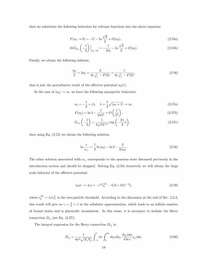
then we substitute the following behaviors for relevant functions into the above equation:

F (ν0 → 0) ∼ −C− ln

√3

2+O(ν0), (2.55a)

2πGν0

(−1

2

) ∣∣∣ν0→0

∼ − 1

2ν0− ln

√3

2+O(ν0). (2.55b)

Finally, we obtain the following solution:

u0

2∼ 2ν0 =

2

ln rα>− F (0)

+1

ln rα<− F (0)

, (2.56)

that is just the perturbative result of the effective potential u0(r).

In the case of |u0| → ∞, we have the following asymptotic behaviors:

ν0 = −1

2+ iλ, λ =

1

2

√|u0 + 1| → ∞, (2.57a)

F (ν0) ∼ lnλ− 1

24λ2+O

(1

λ3

), (2.57b)

Gν0

(−1

2

)∼ 1

2√π31/4

exp

(−2π

3λ

), (2.57c)

then using Eq. (2.52) we obtain the following solution:

lnr

α>=

1

2ln |u0| − ln 2− 2

3|u0|. (2.58)

The other solution associated with α< corresponds to the spurious state discussed previously in the

introduction section and should be dropped. Solving Eq. (2.58) iteratively we will obtain the large

scale behavior of the effective potential:

u0(r →∞) = −r2ε(2)b − 4/3 +O(r−2), (2.59)

where ε(2)b = 4/α2

> is the two-particle threshold. According to the discussion at the end of Sec. 2.2.3,

this result will give us γ = 43 > 1 in the adiabatic approximation, which leads to an infinite number

of bound states and is physically inconsistent. In this sense, it is necessary to include the Berry

connection Dij [see Eq. (2.37)].

The integral expression for the Berry connection Dij is:

Dij =1

8π2√NiNj

∫ 1

−1

dx

∫ 2π

0

dφ1dφ2dχi(n)

d ln rχj(n). (2.60)

19

Using the ansatz for χi(n) of Eq. (2.50) and the Green’s function in Eq. (2.48), we will find that the

Berry connection matrix D is given by:

Dij =(αiαj + 2βiβj)

8π2√NiNj(νi − νj)(νi + νj + 1)

, (2.61)

where the normalization factor Ni of the angular eigenfunctions is calculated to be

Ni =

[(α2i + 2β2

i )∂νiGνi(1) + [2β2i + 4αiβi]∂νiGνi(− 1

2 )]

(4π)(2νi + 1). (2.62)

The details of the derivation of these results can be found in Appendix A. According to Eq. (2.41),

we have the correction to the effective potential of the lowest level as:

∆u0(r →∞) =∑j 6=0

|D0j |2. (2.63)

This can be calculated using the following trick. Firstly, Eq. (2.51) for the eigenstate coefficients (α, β)

can be rewritten in a more compact form:

H(ν)~α = 0, ~α =

α√

2β

, (2.64)

where the 2× 2 matrix Hamiltonian H(ν) is

H(ν) = 2π

1λ1

+Gν(1);√

2Gν(− 1

2

)√

2Gν(− 1

2

); Gν(1) +Gν

(− 1

2

)− 1

λ2

. (2.65)

From Eq. (2.47) and the fact that uj is real, it is easy to verify that H(ν) is a real, symmetric two by

two matrix. Then we must have

det H · H−1 = σyHσy. (2.66)

Since H(ν) has zero eigenvalues, then det H have zeros and H−1 have pole structures:

H−1(ν) =∑j

~αj ⊗ ~αTjν − hj

, (2.67)

where hj is the j-th pole and ~αj is the properly normalized eigenvector of H(ν) corresponding to the

20

j-th pole. As a result, the normalization condition for the eigenstate ~α can be chosen as:

~α⊗ ~αT = σyHσy = det H · H−1. (2.68)

Using the matrix Hamiltonian H(ν) and the normalization condition defined above, we can express

the righthand side of Eq. (2.63) as a contour integration on the complex plane of variable ν:

∑j 6=0

|D0j |2 =1

2

1

2πi

∮Cdν

Tr[Res K(ν0) · K(ν)]

(ν0 − ν)2+

1

2πi

∮Cdν

Tr[Res K(ν∗0 ) · K(ν)]

(ν∗0 − ν)2

, (2.69)

where the matrix function K(ν) is formally defined as K(ν) = H−1(ν). It has poles at where the

matrix Hamiltonian has zeros, and decays rapidly enough when |ν| goes to infinity. The derivation of

this result can be found in Appendix B, and the integration contour is shown in Fig. 2.7.

Re ν

Im ν

Cν1 ν2 ν3 · · ·· · ·

νs

ν0

ν∗s

ν∗0

Figure 2.7: Integration contour for the calculation of ∆u0. The contour is along real axis, where thefirst order poles reside. There are four extra poles far off the real axis, which correspond to true boundstate (ν0) and spurious bound state (νs) respectively. The physical meaning of true bound state andspurious bound state is discussed at the end of the Sec. 2.1

The integration contour can be deformed to enclose the other four poles off the real axis and the

integration can be easily carried out (see Appendix B), leading to the following result:

∆u0 =∑j

|D0j |2 =1

3, (2.70)

which combined with Eq. (2.59) gives us the marginal result γ = 1. This shows the importance of

including Berry connection matrix D and the physical consistency. With this marginal situation, the

existence and property of the three-particle bound state must be handled numerically.

21

Figure 2.8: Eigenvalues of matrix Λ, calculated for energy slightly above (ε+) and below (ε−) the

binding energy ε(3)b . Inset shows result for energy well above ε

(3)b , which is the typical behavior for

spherical waves.

2.3.2 Zero Angular Momentum: Numerics

The numerical implementation of the renormalization group equation (2.36) is simple, it is just a set

of first-order ordinary differential equations and the second-order numerical integration algorithm is

efficient enough for our purpose. The initial matrix Eq. (2.30) is diagonal, the first-order correction

matrix D is anti-symmetric and the effective potential matrix u is diagonal, these conditions guarantee

that during the evolution all eigenvalues of matrix Λ are real as they should be. The algorithm is

divided into two steps: firstly we run the renormalization process at energy slightly below the two-

particle threshold, the existence of three-particle bound state is reflected in the divergence of the

highest eigenvalue of Λ and the number of bound states equals to the number of jumps of the highest

eigenvalue 1 by Levinson’s theorem [68, 31], as discussed at the end of Sec. 2.2.2. Secondly, if the

bound state exists, we further run the renormalization process with varying energies to determine the

binding energy of the three-particle bound state. Typical behaviors of different energies are shown in

Fig. 2.8, where energy slightly above the three-particle binding energy shows a single jump and energy

slightly below the three-particle binding energy shows no divergence. If the energy is well above the

three-particle binding energy, the situation corresponds to a spherical wave, where periodic jumps will

occur at the zeros of the wave function.

The calculation is carried out using MATLAB [69] on a laptop with number of levels included

N = 40. Each run of the renormalization process takes less than 10 minutes 2 and inclusion of more

1Mathematically the divergence is positive on one side of the vertical asymptote and negative on the other side, thusthere is jump from one side to the other side. These jumps are numerically realized by inverting the highest eigenvaluewhile keep the other eigenvalues intact when the former hits a sufficiently large value.

2In the numerical calculation we need to carefully exclude the spurious level as discussed in the introduction section.

22

Table 2.1: Critical values of α> corresponding to different α< when the three-particle bound statedisappear into the two-particle threshold.

α< 0.80 0.82 0.85 0.90 0.95αc> 1.82 1.85 1.90 1.99 2.09

levels only changes the result by less than 1%. For zero angular momentum, there exists at most one

three-particle bound state. At large α>/α< ratio, the ratio between three-particle binding energy

and the two-particle threshold versus α>/α< falls on a universal curve, as illustrated in Fig. 2.9. A

similar universal curve also appears in the case of three-boson all interacting attractively [6, 7, 8].

According to the result for vanishing intraspecies interaction [6, 12], the universal curve in Fig. 2.9

should approach 1.39 asymptotically at infinite α>/α< ratio. Curiously, the convergence to 1.39 is

extremely slow: it only reaches 0.4 for α>/α< = 250, the largest scattering length ratio shown in

Fig. 2.9. In fact, the curve reaches ∼ 1 only for α>/α< ∼ 108 and the correction to 1.39 in the large

α>/α< limit scales as 1/ ln(α>/α<). This curious fact can be partially understood from the first

order perturbation theory with respect to the small parameter f< from Eq. (2.6). It seems that the

result (ε(3)b − ε

(2)b )/ε

(2)b = 1.39 is practically inaccessible due to the logarithmic slow convergence. Into

the region with small α>/α< ratio, universality breaks and the three-particle binding energy merges

into the two-particle threshold at critical values, we listed several critical values in Table 2.1. It’s

notable that our calculation only takes the two scattering lengths α< and α> as input parameters

(see Eq. (2.52)). The microscopic cut-off r0 only appears in the initial condition, where the kinetic

energy dominates and the limit r → 0 can be safely taken (see Eq. (2.30)). These indicate that the

property of the three-particle bound state depends only on the scattering lengths α>, α<, but not on

the microscopic details of the interactions.

æ

æ

ææææææææææ

ææææ

æ

æ

æ

ææ

æ ææ

æ ææ

ææ æ æ

æ æ æ æ ææ æ

ààààà

àààà

àà

à

à

àà

àà

à àà

àà à

à àà à à

à à à à à àà à à à

ììììììììììììì

ì

ìì

ììì

ì

ìììì

ììììì

ìììììììììììììììììì

ìì

50 100 150 200 250

Α>

Α<

0.10

0.15

0.20

0.25

0.30

0.35

0.40

ΕbH3L-Εb

H2L

ΕbH2L

æ Α<=0.5

à Α<=0.6

ì Α<=0.9

Figure 2.9: The universal curve of (ε(3)b − ε

(2)b )/ε

(2)b versus α>/α< at large scattering length ratios.

Data points are collected in the region α>/α< > 10, and with three different values of α<. They fallon the same curve within the numerical accuracy.

23

2.3.3 Non-Zero Angular Momentum

For the solution to Eq. (2.43) with total angular momentum m 6= 0, we first solve for the north pole

n′ = n1 and then rotate the solution to the other two poles. The construction of the Green’s function

can be carried out following the standard procedure of separation of variables:

G(n,n1) = G(x) exp(im1φ1 + im2φ2),

L2 =

[− ∂

∂x(1− x2)

∂

∂x+

m21

2(1− x)+

m22

2(1 + x)

].

(2.71)

In expansion of Green’s function in terms of eigenfunctions of L2, we only need to consider those that

are connected to the δ-function, thus we require m1 = 0 and the eigenfunctions to be regular around

x = −1. These eigenfunctions then can be represented in terms of hypergeometric functions [37]:

L2X(m)j (x) =

(j +

m

2

)(j +

m

2+ 1)X

(m)j (x),

X(m)j (x) =

(1 + x

2

)m/2R

(m)j

(1 + x

2

),

R(m)j (x) = 2F1(−j, j +m+ 1;m+ 1;x),

(2.72)

where m = m1 +m2 = m2 and j takes the value 0, 1, 2, · · · . By using the representation of δ-function

δ(x) =1

2

∞∑j=0

(−)j(2j +m+ 1)Γ(j +m+ 1)

Γ(m+ 1)Γ(j + 1)X

(m)j (x), (2.73)

we immediately obtain the expression for Green’s function:

G(m)νj (n,n1) = (N ·B1)m

1

4 cosπ(νj + 1

2

) Γ(νj +m+ 1)

Γ(νj + 1)Γ(m+ 1)R(m)νj (1−NT A1N) (2.74)

where the four-dimensional vector B1 and 4× 4 matrix A1 are defined as

A1 =

1

1

0

0

, B1 = (0, 0, 1, i)T , (2.75)

24

and N is the following four-dimensional unit vector:

N =

√1−x

2 cosφ′√1−x

2 sinφ′√1+x

2 cosφ′√1+x

2 sinφ′

, (2.76)

where φ′ is an arbitrary phase. To obtain the Green’s function with n′ along the other two poles, we

rotate vector B1 and matrix A1 by 2π/3 on three-dimensional unit sphere, which corresponds to π/3

rotation in four-dimensions. The rotation matrices are as follows:

R2,3 =

12 0 ∓

√3

2 0

0 12 0 ∓

√3

2

±√

32 0 1

2 0

0 ±√

32 0 1

2

. (2.77)

Applying the rotation matrices to the four-dimensional vector B1 and 4× 4 matrix A1 we get:

A2,3 = R2,3A1R−12,3 =

14 0 ±

√3

4 0

0 14 0 ±

√3

4

±√

34 0 3

4 0

0 ±√

34 0 3

4

,

B2,3 = R2,3B1 =

(∓√

3

2,∓√

3

2i, 1/2, i/2

)T.

(2.78)

Substituting the ansatz for eigenfunctions in Eq. (2.44a) with the above specification into Eq. (2.44b),

we will obtain the following constraints on the coefficients (here we add the superscript to emphasize

the dependence on the angular momentum m):

1λ1

+G(m)νj (11); G

(m)νj (12) +G

(m)νj (13)

−G(m)νj (21); 1

λ2−G(m)

νj (22)−G(m)νj (23)

αjβj

= 0, (2.79)

where we have used the shortened notation G(m)νj (lm) ≡ G(m)

νj (nl,nm). Still the equation of spectrum

is obtained via setting the determinant to zero. In order to calculate the involved quantities G(m)νj (lm),

we need to put the three-dimensional unit vectors in Eq. (2.15) back on the four-dimensional unit

25

sphere. This can be done using the following correspondence:

n1 →N1 = (0, 0, cosφ′, sinφ′)T ,

n2,3 →N2,3 =

(∓√

3

2cosφ′,∓

√3

2sinφ′,

1

2cosφ′,

1

2sinφ′

)T,

(2.80)

where φ′ is an arbitrary phase. By direct calculation we will obtain the following results

G

(m)ν (11) = eimφ

′f(ν,m)R

(m)ν (1)

G(m)ν (12) = 1

2m eimφ′f(ν,m)R

(m)ν ( 1

4 )

G(m)ν (13) = 1

2m eimφ′f(ν,m)R

(m)ν ( 1

4 )

,

G

(m)ν (21) = 1

2m eimφ′f(ν,m)R

(m)ν ( 1

4 )

G(m)ν (22) = eimφ

′f(ν,m)R

(m)ν (1)

G(m)ν (23) = (−)m

2m eimφ′f(ν,m)R

(m)ν ( 1

4 )

, (2.81)

where the factor f(ν,m) is defined as

f(ν,m) =1

4 cos[(ν + 1

2

)π] Γ(ν +m+ 1)

Γ(ν + 1)Γ(m+ 1), (2.82)

and R(m)ν (x) has a singularity at x = 1 which is regularized by the finite radius r0:

f(ν,m)R(m)ν (1) =

1

4π

[ln

16

δ−Ψ(−ν)−Ψ(ν +m+ 1) + 2Ψ

(1

2

)],

where δ = r20/r

2 and the Ψ(x) is the digamma function [37]. Putting all these results together, we

finally obtain the equation of spectrum for general value of m:

[ln

r

α<− 1

2M(νj ,m)

][ln

r

α>− 1

2M(νj ,m) + 2π(−)mN(νj ,m)

]= 2[2πN(νj ,m)

]2, (2.83)

with the following definition of the relevant quantities:

M(ν,m) = Ψ(−ν) + Ψ(ν +m+ 1),

N(ν,m) =1

2m1

4 cos[(ν + 1

2

)π] Γ(ν +m+ 1)

Γ(ν + 1)Γ(m+ 1)R(m)ν

(1

4

),

(2.84)

where C = 0.577 · · · is the Euler constant. Specification of Eq. (2.83) to the case m = 0 is just what

we got previously in Eq. (2.52).

We then analyze the large scale behavior of the lowest level. With increasing length scale r, the

angular eigenvalue u0 becomes more and more negative, and the imaginary part of ν0 becomes larger.

26

In the limit |u0| = −u0 →∞, the asymptotic behaviors of the relevant functions [37] are:

M(ν0,m) ∼ ln |u0| − 2 ln 2− 4− 3m2

3|u0|, N(ν0,m) ∼

exp(− 2π

3

√|u0|)

|u0|1/4. (2.85)

Then asymptotically, the equation of spectrum 2.83 reduces to

lnr

α>=

1

2ln |u0| − ln 2− 4− 3m2

6|u0|, (2.86)

where only the solution associated with α> is chosen because the other solution associated with

α< corresponds to the spurious state discussed previously in the introduction section. Solving this

equation iteratively we will get the large scale behavior of the effective potential:

u(m)0 (r →∞) = −r2ε

(2)b + (3m2 − 4)/3 +O(r−2), (2.87)

where ε(2)b = 4/α2

> is the two-particle threshold binding energy. This is the result under adiabatic

approximation.

By performing the asymptotic analysis similar to those for zero angular momentum, we will obtain

the following solution to the effective potential u(m)0 (r) up to first order correction (Appendix B):

u(m)0 (r →∞) = −r2ε

(2)b + (m2 − 1) +O(r−2) (2.88)

thus for non-zero angular momentum, the wave function we will obtain is subject to power-law decay,

and no three-particle bound state is guaranteed at large length scale. To confirm the absence of

three-particle bound state, we need the calculation not only at large length scale, but also in the

intermediate region, which we will still investigate numerically.

The numerical implementation for nonzero angular momentum is essentially the same as that for

zero angular momentum, if we substitute the proper angular eigenfunctions into the corresponding

formulas. Result shows that there is no three-particle bound state for nonzero angular momentum. To

get a sense of what is happening among different m values, we also calculated the effective potential

u0(r)/r2 for the lowest level, the curve has minimum in case of m = 0 while for m > 0 the potential is

monotonously decreasing with increasing r (Fig. 2.10), then it is straightforward to see the possibility

of getting three-particle system bounded for m = 0 and its unlikeness for m > 0.

27

Figure 2.10: Effective Potential u0(r)/r2 for m = 0, 1 with input parameters α> = 20 and α< = 0.5.The dashed line indicates the position of the two-particle threshold.

2.4 Conclusion

In summary, we investigated the existence of three-particle bound states in a two-species, interacting

bosonic system in two dimensions where coupling between like bosons is repulsive and otherwise

attractive. We developed a simple and efficient algorithm via choice of proper parameterization and

base functions. Large scale behavior of the system is handled analytically and interaction region

is handled numerically. Our result shows that there is only one three-particle bound state for zero

angular momentum, and it will merge into the two-particle threshold at small ratio between scattering

lengths (the critical ratio αc>/α< is about 2.2 ∼ 2.3). In contrast, there exist two three-particle bound

states when the couplings between all the three bosons with equal masses are attractive, as investigated

in the literature [13, 6, 7, 8, 12]. For non-zero angular momentum, there is no three-particle bound

state. The two scattering lengths provide enough information to determine the three-particle binding

energy, while the microscopic cut-off r0 and the interaction constants λ1,2 do not enter any way other

than through the scattering lenghts. Our result is in agreement with the previous investigations [6, 64]

in the sense that there are only finite number of three-particle bound states in two dimensions, in

contrast to the condensation of infinite number of three-particle bound states in three dimensions,

and we showed this fact both analytically (the parameter γ define in Eq. (2.42) is equal to or smaller

than unity, which excludes the possibility of infinite number of bound states) and numerically.

Existing approaches for this kind of quantum three-body problem in the literature are mainly

different variations of the Skorniakov-Ter-Martirosian methods. It can be implemented in real space

and solved via the integral equations for the scattering amplitude [78, 81]; or be implemented in

momentum space and solved via the diagrammatic techniques for scattering matrix [12, 63, 52]. It

28

can also be converted into a series of solvable differential equations [77]. All these approaches involve

several numerical integrations over unbounded spaces or kernel inversion, some of them are limited

to s-wave resonant scattering. Here we provide an alternative approach to the quantum three-body

problems, simple and efficient, involving only direct root finding and evolving of a first-order ordinary

differential equation to an intermediate length scale (for example, the divergence behavior showing

the existence of bound state is already clear at a relatively small length scale r ∼ 20 in Fig. 2.8, and

there is no need to evolve the equation further to any larger length scale). It is capable of handling

both short- and long- range physics, free of numerical instability and converges fast enough to avoid

parallelism on clusters. Also our choice of basis via Hopf coordinates reduces the squared proliferation

of hyperspherical harmonics to a linear one with increasing number of included levels, which saves

greatly in numerical endeavor.

29

Chapter 3

Exact Solutions to Two-Component

Many-Body Systems in One

Dimension

3.1 Introduction

In the previous chapter, we have investigated the instability of the condensation in a two-component

system with interspecies attraction and intraspecies repulsion in two dimensions, which is from a

few-body aspect. To gain more insight from the complementary many-body aspect, especially beyond

mean-field and perturbative results, it is worthwhile to construct corresponding models in one di-

mension that is subject to exact solutions. Apart from the theoretical interest, these exactly solvable

models are also of practical value due to the tremendous advances in the experimental realization of

quasi-one dimensional interacting quantum systems using confined cold atoms.

The prototype of one-dimensional exactly solvable models is the famous Lieb-Liniger model [67, 66],

which is now accessible to experimentalists [74, 56, 83, 106]. The two-component models we shall

discuss in the current chapter are multicomponent extensions of the Lieb-Liniger type system [88],

which host a rich spectrum of many-body physics. On the experimental side, such systems have been

realized using different hyperfine states of cold atoms, which provide us with the desired pseudospin

degrees of freedom [108, 71, 3, 65]. The intra- and inter-species interactions can then be tuned via

the Feshbach resonances [16, 28] or external potentials confining the system in one dimension [23, 44].

30

On the theoretical side, the study of exactly solvable models for multicomponent systems begins with

spin 1/2 fermions, which is now known as the Yang-Gaudin model [35, 109, 110]. Sutherland [98] and

Schlottmann [93, 92] then made the generalization to arbitrary spins. The bosonic counterpart was

also studied by various groups [38, 57].

In spite of extensive studies of two-component exactly solvable models in the literature, they

are all limited to the case with a single type of coupling. This is probably due to the fact that

models of simple δ-contact interactions with two different coupling constants fail to fulfill the Yang-

Baxter equation. Here we propose a new type of models for two-component systems with tunable

interspecies interactions, where the Yang-Baxter equation can be fulfilled by fine-tuning the resonant

energies. Although the strict exact solvability beyond the level of two-body scatterings would require

the introduction of extra singular counterterms, the models proposed here can still be well described

by the Bethe ansatz, at least for relatively small densities. It is of relevance not only to experimentally

accessible systems such as bosonic 87Rb quantum gases but also to fundamental theoretical problems

such as BCS-BEC crossover, since, unlike the Yang-Gaudin model, it connects regimes of weakly

attractive atoms to weakly repulsive molecules. Besides, it presents exotic many-body physics of

which in one case the solution is a Fermi sea of two-strings. The remarkable feature is that the

Fermi momentum Q characterizing this sea is limited by the value Q∗, as the increase of the mass

density at fixed interaction is accommodated by the growing density of states of two-strings. A similar

phenomenon was noticed by Gurarie [42] for a single component model with Feshbach resonance, where

the system becomes unstable for small or large interactions. In the other case, an embedded string

solution emerges, which means that the uniform system is unstable and it collapses into a bright

soliton. This collapsing instability happens for fermionic atoms, which is contrary to the intuition

that fermions won’t collapse due to the Pauli exclusion principle.

The remainder of this chapter is organized as follows: In Sec. 3.2 we present the models and

discuss their integrability, then their exact solutions are worked out via the quantum inverse scattering

method [105, 58]. Both bosonic and fermionic cases are considered and we will discover two different

regimes, depending on the competition between inter- and intra-species couplings. In Sec. 3.3 we

discuss the uniform regime with repulsion overcoming attraction, where the ground state properties

and low energy excitations are derived. We also analyze the system with an external magnetic field

in this regime, where a considerable portion of the phase diagram is occupied by the Fulde-Ferrel-

Larkin-Ovchinnikov (FFLO) state [33, 62] and a lower critical magnetic field is found even for large

densities. In Sec. 3.4 we turn to the other regime where the ground state is a bright soliton. Finally,

we summarize the results and discuss possible experimental realizations and extensions.

31

3.2 Models and Their Integrability

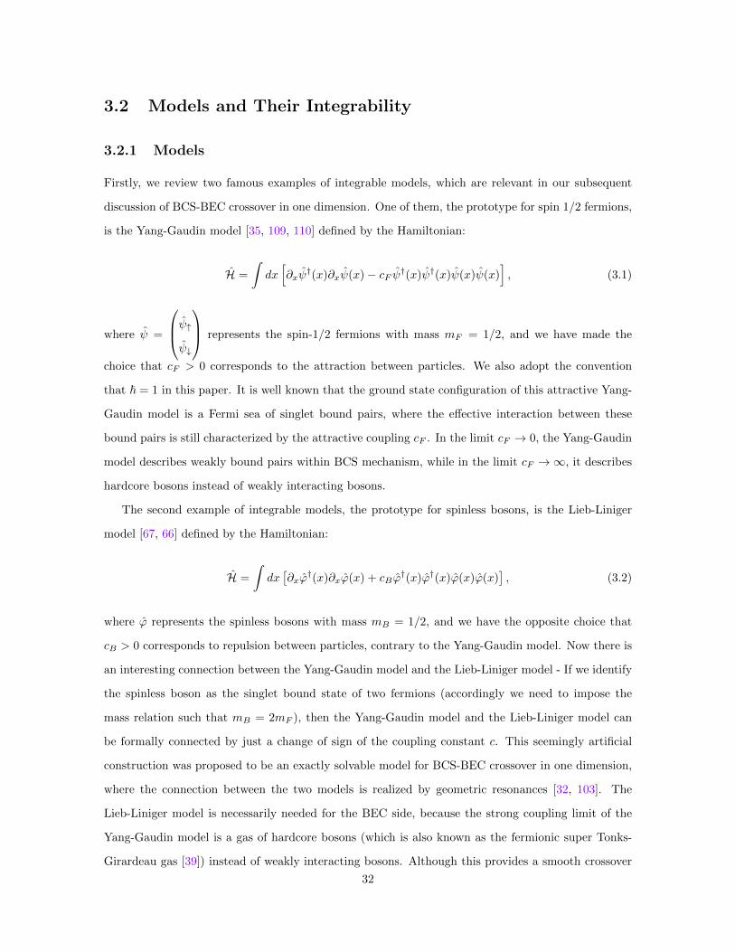
3.2.1 Models

Firstly, we review two famous examples of integrable models, which are relevant in our subsequent

discussion of BCS-BEC crossover in one dimension. One of them, the prototype for spin 1/2 fermions,

is the Yang-Gaudin model [35, 109, 110] defined by the Hamiltonian:

H =

∫dx[∂xψ

†(x)∂xψ(x)− cF ψ†(x)ψ†(x)ψ(x)ψ(x)], (3.1)

where ψ =

ψ↑ψ↓

represents the spin-1/2 fermions with mass mF = 1/2, and we have made the

choice that cF > 0 corresponds to the attraction between particles. We also adopt the convention

that ~ = 1 in this paper. It is well known that the ground state configuration of this attractive Yang-

Gaudin model is a Fermi sea of singlet bound pairs, where the effective interaction between these

bound pairs is still characterized by the attractive coupling cF . In the limit cF → 0, the Yang-Gaudin

model describes weakly bound pairs within BCS mechanism, while in the limit cF →∞, it describes

hardcore bosons instead of weakly interacting bosons.

The second example of integrable models, the prototype for spinless bosons, is the Lieb-Liniger

model [67, 66] defined by the Hamiltonian:

H =

∫dx[∂xϕ

†(x)∂xϕ(x) + cBϕ†(x)ϕ†(x)ϕ(x)ϕ(x)

], (3.2)

where ϕ represents the spinless bosons with mass mB = 1/2, and we have the opposite choice that

cB > 0 corresponds to repulsion between particles, contrary to the Yang-Gaudin model. Now there is

an interesting connection between the Yang-Gaudin model and the Lieb-Liniger model - If we identify

the spinless boson as the singlet bound state of two fermions (accordingly we need to impose the

mass relation such that mB = 2mF ), then the Yang-Gaudin model and the Lieb-Liniger model can

be formally connected by just a change of sign of the coupling constant c. This seemingly artificial

construction was proposed to be an exactly solvable model for BCS-BEC crossover in one dimension,

where the connection between the two models is realized by geometric resonances [32, 103]. The

Lieb-Liniger model is necessarily needed for the BEC side, because the strong coupling limit of the

Yang-Gaudin model is a gas of hardcore bosons (which is also known as the fermionic super Tonks-

Girardeau gas [39]) instead of weakly interacting bosons. Although this provides a smooth crossover

32

between the two pairing schemes, it is not satisfactory because there is no single Hamiltonian governing

the behavior of the system from Eq. (3.1) with cF 1 to Eq. (3.2) with cB 1. Moreover, the

molecule on the BEC side is unbreakable due to the quasi-1D confinement, thus the information of

spin excitations is lost.

To connect the Lieb-Liniger model and the Yang-Gaudin model by a single Hamiltonian, we con-

sider two-component interacting bosons and fermions with tunable interspecies interactions, which will

provide an ideal scenario for one dimensional BCS-BEC crossover without the drawbacks mentioned

above. Generally, the tunable interspecies interaction is realized via Feshbach resonances, where atoms

are bound into molecules. Exact solutions to models with Feshbach resonances are studied in the liter-

ature for one-component interacting particles [42, 51] and for noninteracting fermions in the so-called

quantum three-wave interaction model [107, 85]. Here we make a further step to two-component

interacting systems, where the applicability of Bethe ansatz is obtained by fine-tuning the resonant

energies.

We start by introducing the bosonic model, where the resonance can be viewed as a singlet bound

state (molecule) of two participating bosons. It is defined by the Hamiltonian:

H =

∫dx∂xψ

†∂xψ +∂xΠ†∂xΠ

2mΠ− ε0Π†Π + gψ†ψ†ψψ +

[t

2

(i∂xψ

Tσyψ)

Π† + h.c.

], (3.3)

where ψ =

ψ↑ψ↓

represents the two-component bosons and Π represents the molecules with binding

energy ε0. The matrix σy is the y component of the Pauli matrix σ = (σx, σy, σz). The introduction

of spatial derivatives into the resonant coupling is due to the fact that the spatial part of the bosonic

wave function in the singlet channel has odd parity. Also, we have adopted the convention that

mψ = 1/2, and we have left mΠ unspecified. In fact, the relation between mΠ and mψ is dictated by

Galilean invariance: Under the Galilean transformation

∂t → ∂t − v∂x, ψ → ψe−i

(mψvx+

mψv2

2 t

), Π→ Πe

−i(mΠvx+

mΠv2

2 t

), (3.4)

the action S =∫dxdt

(iψ†∂tψ + iΠ†∂tΠ

)−∫dt H of the system will remain unchanged apart from

a constant shift, provided we impose the relation that mΠ = 2mψ. Thus we can simply substitute

mΠ = 1 into Eq. (3.3). There is one more point that we need to pay attention to, which is the

conservation of particle number. This means that the operator N defined below commutes with the

33

Hamiltonian H:

N =

∫dx

(ψ†ψ + 2Π†Π

), [N , H] = 0. (3.5)

The definition of N takes into account the resonant coupling processes where two bosons with opposite

pseudospin transform into one molecule or vice versa. This commutability can be achieved by imposing

the following commutation relations:

[ψσ(x), ψ†σ′(x′)] = δσσ′δ(x− x′), σ, σ′ =↑, ↓

[Π(x), Π†(x′)] = δ(x− x′),(3.6)

and all the other commutators give out zero.

The fermionic model can be constructed similarly, with the introduction of both scalar and vector

resonances. It is defined by the Hamiltonian:

H =

∫dx

∂xψ

†∂xψ +1

2∂xΞ

† · ∂xΞ +1

2∂xΠ†∂xΠ− εΞΞ† · Ξ− εΠΠ†Π + gψ†ψ†ψψ

+

[tΞ2

(i∂xψ

Tσσyψ)· Ξ† + h.c.

]+

[tΠ2

(iψTσyψ

)· Π† + h.c.

],

(3.7)

where ψ =

ψ↑ψ↓

represents the spin-1/2 fermions, Ξ represents the vector resonances with binding

energy εΞ and Π represents the scalar resonances with binding energy εΠ. Also we adopt the convention

that mψ = 1/2, then mΞ = mΠ = 1 is required by the Galilean invariance, just as what we have

discussed previously. Again we need to be careful about the conservation of particle number:

N =

∫dx

(ψ†ψ + 2Ξ† · Ξ + 2Π†Π

), [N , H] = 0. (3.8)

This can be achieved by imposing the following commutation and anticommutation relations:

ψσ(x), ψ†σ′(x′) = δσσ′δ(x− x′),

ψ†σ(x), ψ†σ′(x′) = 0, ψσ(x), ψσ′(x

′) = 0

[Ξµ(x), Ξ†µ′(x′)] = δµµ′δ(x− x′),

[Π(x), Π†(x′)] = δ(x− x′),

(3.9)

and all the other commutators give out zero. In the above equations, the spin labels σ, σ′ take values

of ↑, ↓, and the polarization labels µ, µ′ take values of +,−, z. The relation between polarization labels

34

and vector labels is as follows:

Ξ+ =1√2

(Ξx + iΞy), Ξ− =1√2

(Ξx − iΞy). (3.10)

The bosonic and fermionic models introduced here can be solved via Bethe ansatz if we fine tune the

resonant energies ε0, εΞ, εΠ, and both of them can be effectively described as a two-component system

with intraspecies repulsion and interspecies attraction. By tuning the strength of attraction from

vanishingly small toward the strength of repulsion, the system first shows BCS-type pairing behavior,

then it develops toward the fermionic super Tonks-Girardeau gas regime, and finally, it turns into the

weakly interacting bosons regime and shows BEC-type pairing behavior. Thus we can have a single

Hamiltonian governing the whole range of BCS-BEC crossover, and there is no geometric confinement

preventing the breaking of bound pairs. What is more, if we tune the strength of attraction beyond

repulsion, we will enter into a new regime where the uniform configuration is unstable and the system

collapses into a bright soliton. Now let us discuss these interesting physics one by one, starting from

the integrability.

3.2.2 Integrability

Figure 3.1: Illustration of the Yang-Baxter equation. It is essentially a requirement of consistencysuch that the two different scattering paths in (1) and (2) give out the same result.

Integrable models with internal degrees of freedom can be solved using the quantum inverse scat-

tering method [105, 58]. The essential point is to construct the two-body S-matrix which fulfills the

Yang-Baxter equation (see Fig. 3.1 for an illustration). For a time inversion and space inversion

invariant and species-conserving model in free space, the two-body S-matrix in pseudospin subspace

35

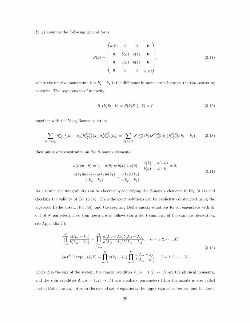
↑, ↓ assumes the following general form:

S(k) =

a(k) 0 0 0

0 b(k) c(k) 0

0 c(k) b(k) 0

0 0 0 a(k)

, (3.11)

where the relative momentum k = k2 − k1 is the difference in momentum between the two scattering

particles. The requirement of unitarity

S†(k)S(−k) = S(k)S†(−k) = I (3.12)

together with the Yang-Baxter equation

∑σ′1σ′2σ′3

Sσ1σ2

σ′1σ′2(k1 − k2)S

σ′1σ3

σ′′1 σ′3(k1)S

σ′2σ′3

σ′′2 σ′′3

(k2) =∑

σ′1σ′2σ′3

Sσ2σ3

σ′2σ′3(k2)S

σ1σ′3

σ′1σ′′3

(k1)Sσ′1σ′2

σ′′1 σ′′2

(k1 − k2) (3.13)

then put severe constraints on the S-matrix elements:

a(k)a(−k) = 1, a(k) = b(k) + c(k),a(k)

b(k)+a(−k)

b(−k)= 2,

a(k1)b(k2)− a(k2)b(k1)

b(k2 − k1)=c(k1)c(k2)

c(k2 − k1).

(3.14)

As a result, the integrability can be checked by identifying the S-matrix elements in Eq. (3.11) and

checking the validity of Eq. (3.14). Then the exact solutions can be explicitly constructed using the

algebraic Bethe ansatz [105, 58], and the resulting Bethe ansatz equations for an eigenstate with M

out of N particles placed spin-down are as follows (for a short summary of the standard derivation,

see Appendix C):

N∏n=1

a(Λα − kn)

b(Λα − kn)=

M∏β=1β 6=α

a(Λα − Λβ)b(Λβ − Λα)

a(Λβ − Λα)b(Λα − Λβ), α = 1, 2, · · · ,M ;

(∓)N−1 exp(−ikjL) =

N∏n=1

a(kj − kn)

M∏α=1

a(Λα − kj)b(Λα − kj)

, j = 1, 2, · · · , N,

(3.15)

where L is the size of the system, the charge rapidities kn, n = 1, 2, · · · , N are the physical momenta,

and the spin rapidities Λα, α = 1, 2, · · · ,M are auxiliary parameters (thus the ansatz is also called

nested Bethe ansatz). Also in the second set of equations, the upper sign is for bosons, and the lower

36

sign is for fermions.

We first review the Bethe ansatz equations for the Yang-Gaudin model and the Lieb-Liniger model

and then turn to the present models defined in Eqs. (3.3) and (3.7). The S-matrix elements for the

Yang-Gaudin model described in Eq. (3.1) are [105, 58]:

a(k) = 1, b(k) =k

k − icF, c(k) =

−icFk − icF

. (3.16)

This clearly fulfills the integrability criterion as specified in Eq. (3.14). Then it is straightforward to

substitute Eq. (3.16) into Eq. (3.15) to obtain the Bethe ansatz equations:

N∏j=1

(Λα − kj − ic′FΛα − kj + ic′F

)= −

M∏β=1

(Λα − Λβ − icFΛα − Λβ + icF

),

exp(ikjL) =

M∏α=1

(kj − Λα − ic′Fkj − Λα + ic′F

),

(3.17)

where c′F = cF /2 and we have made the conventional shift Λα → Λα + ic′F . The ground state

configuration of this attractive Yang-Gaudin model (with even number of particles) is known to be a

Fermi sea of two-string solutions with the structure:

kα,1 = Λα + ic′F , kα,2 = Λα − ic′F , (3.18)

where α = 1, 2, · · · ,M with M = N/2, and the Bethe ansatz equations reduce into equations for the

center momenta Λα:

exp(2iΛαL) = (−)

M∏β=1

(Λα − Λβ − icFΛα − Λβ + icF

). (3.19)

Because the center momenta Λα in the ground state configuration are all real, we can take the

logarithm of the above equations:

2ΛαL = 2πJα −M∑β=1

θ(Λα − Λβ), (3.20)

where Jαs are consecutive integers or half-odd integers depending on:

Jα =M + 1− 2α

2, α = 1, 2, · · · ,M. (3.21)

37

The phase-shift function θ(Λ− Λ′) is defined as:

θ(Λ− Λ′) = −2 arctan

(Λ− Λ′

cF

). (3.22)

In the thermodynamic limit where N →∞, L→∞ with fixed density nF = N/L, Eq. (3.20) can be

replaced by an integral equation for the density of state σ(Λj) = 1/L(Λj+1 − Λj), following Hulten’s

continualization procedure [48]:

σ(Λ) +cFπ

∫ Q

−QdΛ′

σ(Λ′)(Λ− Λ′)2 + c2F

=1

π, (3.23)

where Q is the Fermi momentum of the ground state, and it is determined by the density nF via the

relation:

nF2

=

∫ Q

−QdΛ σ(Λ). (3.24)

After solving the above integral equation, the physical quantities of the ground state can then be

calculated in terms of the density of states σ(Λ).

The Lieb-Liniger model as described in Eq. (3.2) in fact has simpler structure compared with the

Yang-Gaudin model, because it is a single-component model. The resulting ground state configuration

with N particles fulfills the Bethe ansatz equations:

kjL = 2πIj −N∑n=1

θ(kj − kn), (3.25)

where Ijs are consecutive integers or half-odd integers depending on:

Ij =N + 1− 2j

2, j = 1, 2, · · · , N. (3.26)

The corresponding phase-shift function is defined as

θ(k − k′) = 2 arctan

(k − k′cB

), (3.27)

and the integral equation for the density of states ρ(k) = 1/L(kj+1 − kj) in the thermodynamic limit

is:

ρ(k)− cBπ

∫ q

−qdk′

ρ(k′)(k − k′)2 + c2B

=1

2π. (3.28)

38

Similarly q is the Fermi momentum of the ground state 1, and it is determined by the density nB = N/L

via the relation:

nB =

∫ q

−qdk ρ(k). (3.29)

Now it is clear from Eqs. (3.23) and (3.28) that we can formally connect the Yang-Gaudin model and

the Lieb-Liniger model by just a change of sign of the coupling constant c, where the spinless boson

in the Lieb-Liniger model is identified with the singlet bound pair in the Yang-Gaudin model (thus

the requirement that mB = 2mF and nB = 2nF ).

Now we consider the model defined in Eq. (3.3). It can be intuitively understood as follows: The

two-component bosonic atoms denoted by ψ live on hyperplanes corresponding to different ordering

sectors X, where xX1< xX2

< · · · < xXN . Without resonant couplings as in the case of the Yang-

Gaudin and the Lieb-Liniger model, we only need to require the continuity of wave functions when

these hyperplanes intersect. With Feshbach resonances as in our model, the molecules denoted by

Π can be viewed as living on the intersections of the hyperplanes, which play the role of boundary

conditions. As a result, we can describe the system with atomic S-matrices, where the molecules

only enter as appropriate boundary conditions for the atomic wave functions. Next, we calculate the

corresponding S-matrix elements to check the integrability of the present model.

In the triplet channel for ψ-bosons, the Π-boson is not excited, and we have both configuration

(↑↑) and (↑↓ + ↓↑)/√

2. The two-atom states for them are

|two atom〉tri,1 =

∫dx1dx2 φ(x1, x2)ψ†↑(x1)ψ†↑(x2) |0〉 ,

|two atom〉tri,0 =

∫dx1dx2 φ(x1, x2)

ψ†↑(x1)ψ†↓(x2) + ψ†↑(x2)ψ†↓(x1)

2|0〉 .

(3.30)

By acting the S-matrix in Eq. (3.11) on both wave functions, we obtain

S(k) |two atom〉tri,1 = a(k) |two atom〉tri,1 ,

S(k) |two atom〉tri,0 =(b(k) + c(k)

)|two atom〉tri,0 ,

(3.31)

which leads to the result that a(k) = b(k) + c(k). Taking into account that the spatial part of the

wave functions has even parity, we can make the ansatz for φ(x1, x2) = φtri(x2 − x1) such that:

φtri(x) = cos(kx/2 + δtrisgnx), (3.32)

1Interacting one dimensional system has the interesting properties that both bosons and fermions obey the exclusionprinciple: identical particles cannot have the same momentum, otherwise the wave function will vanish. For a detaileddiscussion, see Ref. [58].

39

where δtri is the scattering phase shift. The corresponding Schrodinger equation for φtri(x) can then

be derived from the model Hamiltonian in Eq. (3.3):

(−2∂2x − k2/2)φtri(x) + 2gδ(x)φtri(0) = 0, (3.33)

where φtri(0) ≡ [φtri(0+) + φtri(0

−)]/2 = cos δtri. Integration of Eq. (3.33) around x = 0 gives out

a(k) = b(k) + c(k) = ei2δtri =k − igk + ig

. (3.34)

In the singlet channel for ψ-bosons, the Π-boson is also excited. The general form of the two-atom

state in this case can be expressed as:

|two atom〉sin =

∫dy Φ(y)Π†(y) |0〉+

∫dx1dx2 φ(x1, x2)

ψ†↑(x1)ψ†↓(x2)− ψ†↑(x2)ψ†↓(x1)

2|0〉 . (3.35)

Based on symmetry considerations, the following ansatz for φ(x1, x2) and Φ(y) is appropriate:

φ(x1, x2) = φsin(x2 − x1)eiK(x1+x2), Φ(y) = Φ e2iKy, (3.36)

where K is the momentum of the mass center and the singlet wave function has odd parity

φsin(x) = sin(kx/2 + δsinsgnx). (3.37)

Then the corresponding Schrodinger equation is:

(−2∂2x − k2/2)φsin(x) + t∗δ′(x)Φ = 0,

− ε0Φ− t∂xφ(x)∣∣∣x→0+

= k2Φ/2,

(3.38)

which gives the expression for the S-matrix element in the singlet channel

b(k)− c(k) = e2iδsin =4(k2 + 2ε0)− i|t|2k4(k2 + 2ε0) + i|t|2k . (3.39)

Equation (3.39) together with Eq. (3.34) give us the expression of matrix elements specified in

Eq. (3.11). Substituting them into the requirement in Eq. (3.14), we finally arrive at the follow-

40

ing condition for integrability of the present model defined in Eq. (3.3):

2ε0 = g(g − |t|2/4). (3.40)

This can be achieved by fine tuning the resonant energy ε0. We further introduce new coupling

constants c1, c2 as:

c1 = g, c2 = 2ε0/g, (3.41)

such that the S-matrix elements take the simple form

a(k) =k − ic1k + ic1

,b(k)

a(k)=

k

k − ic2. (3.42)

In the case with repulsive intraspecies coupling c1 > 0, the sign of c2 is controlled by the resonant

energy ε0. The choice c2 > 0 introduces a interspecies attraction resulting a physical pole in the

singlet channel, which is exactly the singlet bound state with binding energy ε0 > 0 that we have in

mind when proposing the model. Furthermore from Eq. (3.40) we can infer the competition between

the two coupling constants:

c1 − c2 = |t|2/4 > 0. (3.43)

Above we only considered two-body scatterings defined by the Hamiltonian in Eq. (3.3) and we

showed that the model can be made integrable by fine-tuning the resonant energy if only two-body

scatterings are important. Strictly speaking, this is not sufficient for the integrability when we consider

three-body and four-body scatterings (in particular, the resulting wave functions for the three-atom

sector have discontinuities when a Π particle sits right on top of a ψ particle). In another word, the

Π-ψ and Π-Π scatterings cannot be factorized into successive two-body scatterings. Practically, at

least for relatively small densities of the system, the effect of three-body and four-body scatterings is

negligible compared with two-body scatterings, since Π particles live only on the intersections of the

hyperplanes and their scatterings are of measure zero. This is in the spirit of the so-called asymptotic

Bethe ansatz [98, 42, 51]. It is also possible to save the factorizability by introducing counterterms

to the quadratic spectrum, as what has been done for the exact solution to the multichannel Kondo

model [91, 4]. This recipe can be made local and Galilean invariant, for example, the counter terms

to be added to the Hamiltonian are

Hcounter =1

2

∫dx

[Tx(∂xΠ†ψ†ψΠ− 2Π†∂xψ

†ψΠ + ∂xΠ†Π†ΠΠ)

+ h.c.], (3.44)

41

where the jumping operator Tx on two-body interaction terms is defined as

Tx[A†B†CD

]≡[A†(x)B†(x′)C(x)D(x′)

]x′=x−0

−[A†(x)B†(x′)C(x)D(x′)

]x′=x+0

. (3.45)

Although these counterterms save the factorizability when the resonance is turned on (t 6= 0), they

pose the problem of producing a continuum of bound states when the resonance is turned off (t = 0),

and we don’t know what will become of these bound states once the resonance is turned on. Here we

disregard all these complexities and use the S-matrix specified in Eq. (3.42) to construct the Bethe

ansatz. We believe this captures the essential features of the model as the corresponding Bethe ansatz

equations give out physically sensible results.

Before entering into the standard process of quantum inverse scattering method of solving the

bosonic model, we also check the integrability of the fermionic model described in Eq. (3.7) on the

two-body scattering level, disregarding the complexities discussed above. Then the same S-matrix

elements in Eq. (3.42) are obtained for the fermionic model but with the possibility of c1 < c2. We

follow the same procedure as the bosonic case. The corresponding Schrodinger equation in the triplet

channel is then

(−2∂2x − k2/2)φtri(x) + t∗Ξδ

′(x)ΦΞ = 0,

− εΞΦΞ − tΞ∂xφtri(x)x→0+ = k2ΦΞ/2,

(3.46)

where φtri(x) = sin(kx/2 + δtrisgnx) is the spatial part of the triplet wave function and ΦΞ is the

amplitude of the vector resonance wave function. We then obtain the S-matrix element in the triplet

channel:

a(k) = b(k) + c(k) = e2iδtri =4(k2 + 2εΞ)− i|tΞ|2k4(k2 + 2εΞ) + i|tΞ|2k

. (3.47)

Similarly, in the singlet channel we have the following Schrodinger equation:

(−2∂2x − k2/2)φsin(x) + [2gφsin(0) + t∗ΠΦΠ]δ(x) = 0,

− εΠΦΠ + tΠφsin(0) = k2ΦΠ/2,

(3.48)

where φsin(x) = cos(kx/2 + δsinsgnx) is the spatial part of the singlet wave function and ΦΠ is the

amplitude of the scalar resonance wave function. We then obtain the S-matrix element in the singlet

channel:

b(k)− c(k) = e2iδsin =k(k2 + 2εΠ)− i[gk2 + 2gεΠ + |tΠ|2]

k(k2 + 2εΠ) + i[gk2 + 2gεΠ + |tΠ|2]. (3.49)

42

Equation (3.47) together with Eq. (3.49) produce the same S-matrix elements in Eq. (3.42) if the

following fine tuning is applied:

εΞ = 0,|tΞ|2

4

( |tΞ|24− g)

= −|tΠ|2

g= 2εΠ, (3.50)

and the coupling constants c1, c2 are defined as:

c1 = |tΞ|2/4, c1 − c2 = −|tΠ|2/(2εΠ). (3.51)

If the scalar resonance is made a singlet bound state with binding energy εΠ > 0, then we realize the

possibility of c1 < c2 mentioned above.

Since both the bosonic and fermionic model present the same form of S-matrix elements in

Eq. (3.42), we can discuss their exact solutions together by substituting Eq. (3.42) into Eq. (3.15).

The resulting algebraic Bethe ansatz equations in the sector where M out of N atoms are placed

spin-down are:

(−)

N∏n=1

Λα − kn − ic′2Λα − kn + ic′2

=

M∏β=1

Λα − Λβ − ic2Λα − Λβ + ic2

,

(∓)N−1e−ikjL =

N∏n=1

kj − kn − ic1kj − kn + ic1

M∏α=1

Λα − kj − ic′2Λα − kj + ic′2

,

(3.52)

where L is the size of the system, c′2 = c2/2, j, n = 1, 2, · · · , N and α, β = 1, 2, · · · ,M . The conven-

tional shift Λα → Λα + ic′2 is introduced. Also the upper sign is for bosons, and the lower sign is

for fermions. In the following sections we discuss the two cases with c1 > c2 > 0 and c2 > c1 > 0

respectively.

3.3 Uniform Regime with c1 > c2 > 0

In this section, we discuss the present model in the parameter regime c1 > c2 > 0, where the ground

state is a Fermi sea of the two-atom bound pair. Firstly, we derive the equation for the density of

states in the thermodynamic limit, where we analyze its singular behavior due to level condensation

and find that the Fermi momentum is bounded from above. Then we discuss the physics of BCS-BEC

crossover in the context of the present model, where we find that the extremes of the excitation spectra

have robust features and the system develops a collapsing instability in the limit c2 → c1. After that,

we discuss the zero temperature phase diagram of the present model with an external magnetic field,

43

of which a considerable part is occupied by the one dimensional analog of the FFLO state. Besides, a

critical magnetic field arises due to the presence of the upper bound for the Fermi momentum. This is

in contrast to the situation for the Yang-Gaudin model, where an arbitrarily small external magnetic

field can polarize the ground state as long as the particle density of the system is large enough.

3.3.1 Level Condensation and Limiting Fermi Momentum Q∗

Let us start with the system with even number of atoms. Then the ground state is a Fermi sea of

two-strings with the same structure as in the Yang-Gaudin model:

kα,1 = Λα + ic′2, kα,2 = Λα − ic′2, (3.53)

where α = 1, 2, · · · ,M = N/2 and the Bethe ansatz equations in Eq. (3.52) reduce to the equations

for the center momenta Λα:

ei2ΛαL = (−)

M∏β=1

(Λα − Λβ − ic2Λα − Λβ + ic2

)(Λα − Λβ + ic1Λα − Λβ − ic1

)2

(Λα − Λβ + i(c1 + c2)

Λα − Λβ − i(c1 + c2)

)(Λα − Λβ + i(c1 − c2)

Λα − Λβ − i(c1 − c2)

).

(3.54)

Because the center momenta Λα in the ground state are all real, we can take the logarithm of the

above equations:

2ΛαL = 2πJα −M∑β=1

θ(Λα − Λβ), (3.55)

where Jαs are consecutive integers or half-odd integers depending on:

Jα =M + 1− 2α

2, α = 1, 2, · · · ,M. (3.56)

The phase-shift function θ(Λ− Λ′) is defined as:

θ(Λ−Λ′) = −2 arctan

(Λ− Λ′

c2

)+ 4 arctan

(Λ− Λ′

c1

)+ 2 arctan

(Λ− Λ′

c1 + c2

)+ 2 arctan

(Λ− Λ′

c1 − c2

).

(3.57)

We can see that Eq. (3.57) reduces to Eq. (3.22) in the limit c2 1 c1, and to Eq. (3.27) in the

limit 0 < c1 − c2 1 c1, so the present model has the Yang-Gaudin model and the Lieb-Liniger

model as its two limiting models. Also the total energy and momentum of the system can then be

44

expressed as:

E =

M∑α=1

[(Λα +

ic22

)2

+

(Λα −

ic22

)2], P =

M∑α=1

2Λα. (3.58)

In the thermodynamic limit, Eq. (3.55) can be replaced by an integral equation for the density of

state σ(Λj) = 1/[L(Λj+1 − Λj)], just like what we have discussed previously:

σ(Λ)−∫ Q

−QdΛ′ K(Λ− Λ′)σ(Λ′) =

1

π, K(Λ− Λ′) =

1

2πθ′(Λ− Λ′), (3.59)

where Q is the Fermi momentum of the ground state, and it is determined by the density n = N/L

via the relation:

n

2=

∫ Q

−QdΛ σ(Λ). (3.60)

Also the total energy and momentum of the system in the thermodynamic limit can be expressed

using the density of state σ(Λ):

E =

∫ Q

−QdΛ

(2Λ2 − c22

2

)σ(Λ), P =

∫ Q

−QdΛ 2Λσ(Λ). (3.61)

For further analysis of Eq. (3.59), it is useful to rescale the parameters with respect to Q:

x ≡ Λ

Q, λ ≡ c1

Q, ξ ≡ c2

c1. (3.62)

Correspondingly, the integral equation for the density of states with the rescaled parameters is:

σ(x)−∫ 1

−1

dx′ K(x− x′)σ(x′) =1

π, (3.63)

where K(x) expressed in the rescaled parameters is

K(x) =1

π

(− ξλ

x2 + (ξλ)2+

2λ

x2 + λ2+

(1 + ξ)λ

x2 + (1 + ξ)2λ2+

(1− ξ)λx2 + (1− ξ)2λ2)

), (3.64)

and Eq. (3.60) is equivalent to ∫ 1

−1

dx σ(x) =n

2Q. (3.65)

By construction, the density of states σ(x) > 0 for x ∈ [−1, 1]. Correspondingly, the kernel

L(x, x′) = δ(x− x′)−K(x− x′) (3.66)

45

in Eq. (3.63) must also be a positive definite operator, with its smallest eigenvalue bigger than

1/(πσmax), where σmax is the maximum value of σ(x) on the interval x ∈ [−1, 1] [58]. This is in-

deed the case in the Lieb-Liniger model and the Yang-Gaudin model for any coupling strength.

However, in the present model, the kernel L(x, x′) in Eq. (3.66) is positive definite only for λ >

λ∗ = λ∗(ξ), where λ∗(ξ) will be found later. Equivalently, Eq. (3.62) yields an upper bound for the

Fermi momentum:

Q < Q∗ = c1/λ∗. (3.67)

Then, the apparent conflict appears: How do we satisfy the conservation of the mass density of the

system in Eqs. (3.60) and (3.65) while the Fermi momentum Q is limited by Q∗? Solution of this

problem is to have σ(x)→∞ at n→∞ while keeping Q∗ fixed. The only way to have such a result

is to require the operator L(x, x′) to have an almost zero mode at λ→ λ∗ + 0:

∫ 1

−1

dx′Lλ∗(x, x′)σ0(x) = 0. (3.68)

This phenomenon reminds us the condensation of levels which is characteristic for weakly interacting

bosons (see Fig. 3.2).

Figure 3.2: Condensation of levels for weakly interacting bosons in one dimension. Left pane is drawnfor strong coupling and right pane is draw for weak coupling.

For a fixed value of ξ and different values of λ, we solve Eq. (3.63) numerically using the modified

quadrature method [86], where the usual quadrature approximation to the integral is modified to give

more accurate result for a weakly singular kernel. The critical value λ∗(ξ) is determined by the point

at which the value of the solution σ(x) to Eq. (3.63) changes from positive to negative. Accordingly, for

a fixed value of ξ, the zero mode σ0(x) for Lλ∗(x, x′) can be approximated by the singular part of the

solution σ(x) that grows with increasing density n when λ→ λ∗(ξ) + 0. The numerically determined

46

critical curve λ∗(ξ) is shown in Fig. 3.3, which has the limiting behavior that λ∗(ξ → 0) ≈ 0.88 and

λ∗(ξ → 1) → ∞. In the latter limit, the upper bound Q∗ goes to zero and the system develops a

collapsing instability which we will discuss in Sec. 3.4. Also the critical curve λ∗(ξ) can be fitted by

0.0 0.2 0.4 0.6 0.8 1.0ξ

1

2

3

4

5

6

7λ*

Figure 3.3: The critical value λ∗ as a function of ξ = c2/c1. The dots are obtained numerically andthe thick line is the curve of the fitting function in Eq. (3.69). We can see that as ξ → 1, λ∗ → ∞,which means that Q∗ tends to zero, this implies the instability of the system.

the following formula:

λ∗(ξ) =

√0.75

1− ξ + 0.015 + 0.045ξ + 0.50ξ2, ξ ∈ (0, 1), (3.69)

The solution σ(x) to Eq. (3.63) at λ → λ∗ + 0 for several values of ξ is shown in Fig. 3.4, and it

consists of a regular and a singular part:

σ(x) = σreg(x) + σ0(x), (3.70)

where the singular part σ0(x) can be viewed as the approximated zero mode defined in Eq. (3.68),

thus we use the same symbol for them.

In the limit ξ → 1, we can extract the analytical expression for the zero mode from Eq. (3.63).

For ξ → 1, we have (1− ξ)λ∗(ξ)→ 0 from Eq. (3.69), then K(x− x′) in Eq. (3.64) at λ→ λ∗ + 0 can

be approximated as

K(x− x′) ≈ 1

π

(3

2λ+

(1− ξ)λ(x− x′)2 + (1− ξ)2λ2

),

≈ 3

2πλ+ δ(x− x′)− (1− ξ)λ

π

∂

∂xP 1

x− x′ ,(3.71)

where the symbol P represents the Cauchy principle part. As a result, Eq. (3.63) can be reduced to

47

Figure 3.4: The solution σ(x) to Eq. (3.63) for λ→ λ∗(ξ) + 0. σ(x) can be separated into the regularpart σreg(x) and the singular part σ0(x), where the latter grows with increasing n and is seen in thefigure as the part near x = 0.

an equation for the zero mode σ0(x):

− 3

2πλ

∫ 1

−1

dx′σ0(x′) +(1− ξ)λ

π

∂

∂xP∫ 1

−1

dx′σ0(x′)x− x′ =

1

π. (3.72)

Using the identity that

P∫ 1

−1

dx′

x− x′√

1− x′2 = πx, (3.73)

the solution σ0(x) to Eq. (3.72) can be determined as

σ0(x) =4λ

π

1

4(1− ξ)λ2 − 3

√1− x2, (3.74)

where the value of λ is then fixed by the normalization condition in Eq. (3.65):

∫ 1

−1

dx′σ0(x′) =n

2Q=

n

2c1λ. (3.75)

The critical value λ∗ is given by either the condition that σ0(x) > 0 or by Eq. (3.75) in the limit

n→∞:

λ∗ =

√3

4(1− ξ) , (3.76)

which agrees with the fitting formula in Eq. (3.69) in the limit ξ → 1. Using Eq. (3.76), we can rewrite

σ0(x) in Eq. (3.74) as

σ0(x) =4λλ∗2

3π

√1− x2

λ2 − λ∗2=

2c13π

√1− x2

Q∗ −Q , (3.77)

48

where Q = c1/λ and Q∗ = c1/λ∗. This square root singularity in σ0(x) also appears in the Lieb-Liniger

model when the coupling constant cB approaches zero from the positive side [67, 49]. Here it appears

in the limit ξ → 1 when Q approaches Q∗ from below. The difference is that in the Lieb-Liniger

model, the Fermi momentum Q grows with increasing density n, while in the present model the Fermi

momentum is bounded from above with increasing density n, so the present model provides a more

proper realization for BEC in one dimension.

For ξ smaller than 1, the zero mode σ0(x) acquires correction to the form in Eq. (3.77) near the

boundaries x = ±1 (see Fig. 3.4). Numerical calculation shows that this correction is negligible up to

the point ξ = 0.4, so the functional form in Eq. (3.77) provides a good description of the zero mode

σ0(x) in the range 0.4 < ξ < 1, and we only need to replace the prefactor 2c1/(3π) with a positive

function F (Q∗) that depends on Q∗.

Far away from the lower bound λ∗, asymptotic behaviors for the density of state σ(x) can be

extracted from Eq. (3.63) in the limit λ → ∞ with limξ→0 ξλ → 0 and limξ→1(1 − ξ)λ → 0. For

ξ → 0, Eq. (3.63) reduces to

σ(x) +1

π

∫ 1

−1

dx′ξλ

(x− x′)2 + (ξλ)2σ(x′) =

1

π, (3.78)

which coincides Eq. (3.23) for the Yang-Gaudin model if we rescale the parameters there accordingly.

The asymptotic behavior for the solution σ(x) to Eq. (3.78) in the limit ξλ → 0 has already been

obtained in literature [36, 50]:

σ(x) =1

2π

(1 +

ξλ

π

1

1− x2+ · · ·

). (3.79)

For ξ → 1, Eq. (3.63) reduces to

σ(x)− 1

π

∫ 1

−1

dx′(1− ξ)λ

(x− x′)2 + (1− ξ)2λ2σ(x′) =

1

π, (3.80)

which coincides Eq. (3.28) for the Lieb-Liniger model if we rescale the parameters there accordingly.

The asymptotic behavior for the solution σ(x) to Eq. (3.80) in the limit (1 − ξ)λ → 0 has also been

obtained in the literature [49, 36]:

σ(x) =1

π(1− ξ)λ√

1− x2 +1

2π2

1√1− x2

[x ln

(1− x1 + x

)+ ln

16πe

(1− ξ)λ

]+ · · · . (3.81)

The two asymptotic behaviors in Eqs. (3.79) and (3.81) will be of use in the next section when we

49

calculate the asymptotic behaviors of physical observables in the BCS and BEC limits of the present

model.

3.3.2 BCS-BEC Crossover without External Magnetic Field

We will now show that the present model can provide an ideal scenario for BCS-BEC crossover in one

dimension, without the drawbacks of simply connecting Yang-Gaudin model with Lieb-Liniger model.

The behavior of the system is controlled by two dimensionless coupling constants:

γ1 = c1/n, γ2 = c2/n, (3.82)

where mψn = mψN/L is the total mass density of the system with mψ being the mass of the atom.

The ratio between the two dimensionless coupling constants is γ2/γ1 = ξ.

We consider the situation that γ1 1 is kept fixed at a large value and γ2 is varied such that ξ

goes from 0 to 1. In the limit ξ → 0, the dominant term in Eq. (3.57) is:

θ(Λ− Λ′) ≈ −2 arctan

(Λ− Λ′

c2

), (3.83)

which coincides with the Yang-Gaudin model (see Eq. (3.22)). Thus the BCS limit can be realized by

tuning γ2 to the limit ξ → 0, where the system is weakly coupled with small dimensionless coupling

γ2. As we tune the coupling γ2 larger, the system evolves toward the fermionic super Tonks-Girardeau

gas, where the Yang-Gaudin model terminates. If we tune the coupling γ2 even larger, the system can

overcome this strong coupling limit and develop bosonic behaviors. In the limit ξ → 1, the dominant

term in Eq. (3.57) is:

θ(Λ− Λ′) ≈ 2 arctan

(Λ− Λ′

c1 − c2

), (3.84)

which coincides with the Lieb-Liniger model (see Eq. (3.27)). Thus the BEC limit is realized by tuning

γ2 to the limit ξ → 1, where the system is again weakly coupled with small dimensionless coupling

δγ = γ1−γ2. We can see that the present model describes the BCS-BEC crossover in a unified fashion,

with a single Hamiltonian governing the evolution.

The crossover between fermionic and bosonic behaviors can be demonstrated by the evolution

of density of states σ(x) with varying γ2. The asymptotic behaviors of σ(x) in the BCS and BEC

limits are shown in Eqs. (3.79) and (3.81), and a typical result of σ(x) obtained by solving Eq. (3.63)

together with Eq. (3.65) numerically is shown in Fig. 3.5, where the crossover between flat distribution

in BCS limit and level condensation in BEC limit is transparent. Next, we discuss the ground state

50

Figure 3.5: Density of states σ(x) with fixed γ1 and varying γ2, where γ1,2 ≡ c1,2/n. By tuningγ2 toward γ1, the behavior of the system changes from weakly attractive fermions (nearly fat at thecenter and sharp increase near the boundary) to fermionic super Tonks-Girardeau gas and finally toweakly interacting bosons (condensation at the center).

properties and low energy excitations of the present model at BCS-BEC crossover respectively.

3.3.2.1 Ground State Properties and Instability

We analyze the ground state energy and further the compressibility of the system. The ground state

energy density ε and conserved density n can be calculated using the density of states σ(x):

ε =E

L=

∫ Q

−QdΛ

(2Λ2 − c22

2

)σ(Λ) = Q3

∫ 1

−1

dx

(2x2 − ξ2λ2

2

)σ(x),

n =N

L=

∫ Q

−QdΛ 2σ(Λ) = Q

∫ 1

−1

dx 2σ(x),

(3.85)

and the compressibility κ can be calculated from the energy density ε using the standard thermody-

namic relation:

1

κ= n2

(d2ε

dn2

). (3.86)

The asymptotic behaviors of ε and κ in the BCS (ξ → 0) and BEC (ξ → 1) limits are obtained by

51

Figure 3.6: Numerical result for compressibility, where we have made it dimensionless by multiplyingby n3. Left panel is plotted for the present model with γ1 = 5, where κn3 changes with ξ = c2/c1.Right panel is plotted for the Yang-Gaudin model by varying dimensionless coupling constant γ =cF /n. The difference is apparent: for the present model, there is divergence for compressibility, whilefor the Yang-Gaudin model, the compressibility saturates at a finite value.

substituting Eqs. (3.79) and (3.81) into Eqs. (3.85) and (3.86):

ε+ nc22/4

nεF

ξ→0≈ 1

3

(1− 6γ1

π2ξ + · · ·

),

ε+ nc22/4

nεF

ξ→1≈ γ1(1− ξ)π2

(1− 8

√γ1(1− ξ)

3π+ · · ·

),

1

κn3

ξ→0≈ π2

2

(1− 2γ1

π2ξ + · · ·

),

1

κn3

ξ→1≈ γ1(1− ξ)2

(1−

√γ1(1− ξ)π

+ · · ·).

(3.87)

where εF = π2n2/4 is the Fermi energy for the noninteracting Fermi gas and c22/4 is the binding energy

per atom. The results in Eq. (3.87) agree with those for the Yang-Gaudin model and the Lieb-Liniger

model in the weak coupling limit respectively [67, 59, 32].

For general values of ξ, we numerically solve Eq. (3.63) for the density of states σ(x) and numer-

ically calculate the ground state energy and compressibility. A typical result for the compressibility

is shown in Fig. 3.6, together with the result for the Yang-Gaudin model for a comparison. From

Fig. 3.6, we can see that instead of saturating at a finite value as in the Yang-Gaudin model, the

compressibility of the system in the present model diverges in the limit ξ → 1, just as shown by

the asymptotic behavior in Eq. (3.87). This means that the system becomes infinitely compressible

and the spatially uniform ground state becomes unstable. In the meantime, the upper bound Q∗ for

the Fermi momentum goes to zero in the same limit (see Fig. 3.3). These facts signal a collapsing

instability in the system, which we will discuss in the Sec. 3.4.

3.3.2.2 Excitations and Robustness of Their Extremes

We analyze the low energy excitations of the present model. There are two types of them, classified

according to the spin quantum number - the S = 0 excitations and the S = 1/2 excitations. We first

52

summarize their features and then present the detailed analysis.

The spectrum of the S = 0 excitations in the present model has two branches, one of them is

the usual Bogoliubov quasiparticle branch and the other is similar to the type-II branch in the Lieb-

Liniger model [66]. Physically, the former can be identified as the particle branch and the latter can

be identified as the hole branch (see Fig. 3.7), a classification due to the fact that the structure

of the ground state is the same as that of a Fermi system. There are two robust features for the

second branch: The maximum energy is achieved at kmax = kF = πn/2 and there is a periodicity of

2kF = πn, where kF is the Fermi momentum for the noninteracting Fermi gas. These two features

are robust against the variations of the dimensionless coupling strength γ1 and γ2.

particle type

hole type

ϵ=vck k=π nk=π n

2

0.5 1.0 1.5 2.02k/(π n)

0.5

1.0

1.5

2.0

ϵ/n2γ1=2.62,γ2=1.31

Figure 3.7: A typical spectrum for the S = 0 excitations. There are two branches, one for hole typeand one for particle type. At long wavelength, they both reduce to the phonon branch. The maximumof the hole branch is fixed at kmax = kF = πn/2 and there is a periodicity of 2kF = πn in the holebranch.

The spectrum of the S = 1/2 excitations in the present model is similar to that in the Yang-Gaudin

model (see Fig. 3.8). It is gapped and also has a robust extreme: The minimum energy is achieved

at kmin = kF = πn/2, robust against variations of the dimensionless coupling strength γ1 and γ2.

This is in sharp contrast to the situation in higher dimensions, where the momentum of the minimum

energy can be shifted from kF on the deep BCS side to zero on the deep BEC side [76]. This is also

counterintuitive in the sense that there is no conservation law to guarantee this robustness as in the

Luttinger theorem, since there is tunneling between atoms and molecules back and forth.

The calculation of low energy excitations for exactly solvable models follows a standard procedure

[105, 58]. The idea is as follows: The low energy excitations can be excited by various perturbations

to the ground state. Since in the thermodynamic limit, the integral equations for the perturbations

are linear, we can make a clever choice of linear combinations of the perturbations to give out phys-

53

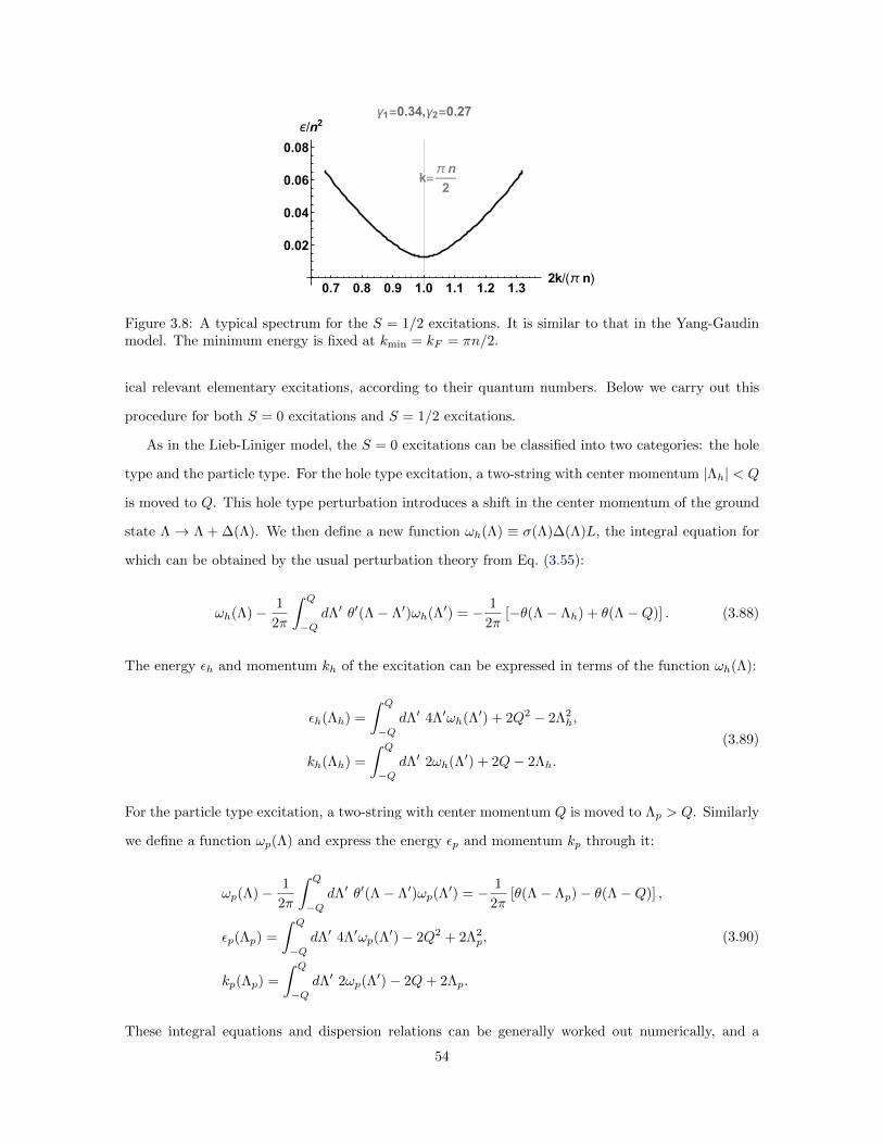
k=π n

2

0.7 0.8 0.9 1.0 1.1 1.2 1.32k/(π n)

0.02

0.04

0.06

0.08

ϵ/n2γ1=0.34,γ2=0.27

Figure 3.8: A typical spectrum for the S = 1/2 excitations. It is similar to that in the Yang-Gaudinmodel. The minimum energy is fixed at kmin = kF = πn/2.

ical relevant elementary excitations, according to their quantum numbers. Below we carry out this

procedure for both S = 0 excitations and S = 1/2 excitations.

As in the Lieb-Liniger model, the S = 0 excitations can be classified into two categories: the hole

type and the particle type. For the hole type excitation, a two-string with center momentum |Λh| < Q

is moved to Q. This hole type perturbation introduces a shift in the center momentum of the ground

state Λ → Λ + ∆(Λ). We then define a new function ωh(Λ) ≡ σ(Λ)∆(Λ)L, the integral equation for

which can be obtained by the usual perturbation theory from Eq. (3.55):

ωh(Λ)− 1

2π

∫ Q

−QdΛ′ θ′(Λ− Λ′)ωh(Λ′) = − 1

2π[−θ(Λ− Λh) + θ(Λ−Q)] . (3.88)

The energy εh and momentum kh of the excitation can be expressed in terms of the function ωh(Λ):

εh(Λh) =

∫ Q

−QdΛ′ 4Λ′ωh(Λ′) + 2Q2 − 2Λ2

h,

kh(Λh) =

∫ Q

−QdΛ′ 2ωh(Λ′) + 2Q− 2Λh.

(3.89)

For the particle type excitation, a two-string with center momentum Q is moved to Λp > Q. Similarly

we define a function ωp(Λ) and express the energy εp and momentum kp through it:

ωp(Λ)− 1

2π

∫ Q

−QdΛ′ θ′(Λ− Λ′)ωp(Λ

′) = − 1

2π[θ(Λ− Λp)− θ(Λ−Q)] ,

εp(Λp) =

∫ Q

−QdΛ′ 4Λ′ωp(Λ

′)− 2Q2 + 2Λ2p,

kp(Λp) =

∫ Q

−QdΛ′ 2ωp(Λ

′)− 2Q+ 2Λp.

(3.90)

These integral equations and dispersion relations can be generally worked out numerically, and a

54

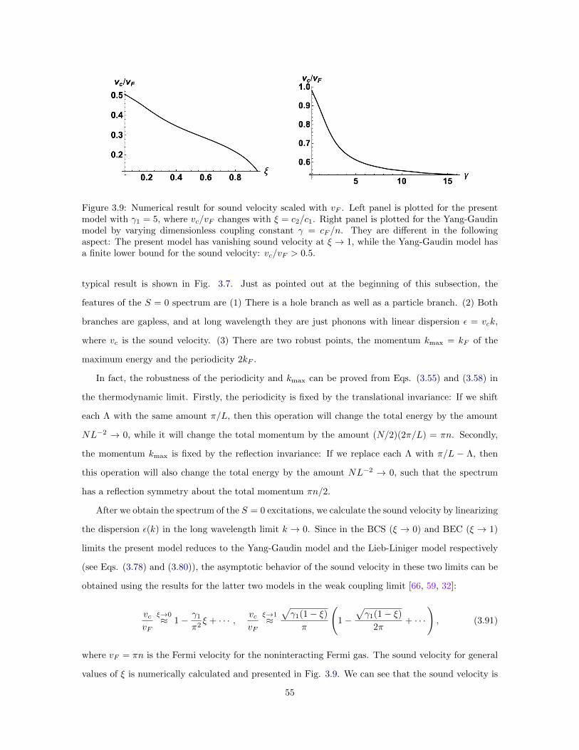
Figure 3.9: Numerical result for sound velocity scaled with vF . Left panel is plotted for the presentmodel with γ1 = 5, where vc/vF changes with ξ = c2/c1. Right panel is plotted for the Yang-Gaudinmodel by varying dimensionless coupling constant γ = cF /n. They are different in the followingaspect: The present model has vanishing sound velocity at ξ → 1, while the Yang-Gaudin model hasa finite lower bound for the sound velocity: vc/vF > 0.5.

typical result is shown in Fig. 3.7. Just as pointed out at the beginning of this subsection, the

features of the S = 0 spectrum are (1) There is a hole branch as well as a particle branch. (2) Both

branches are gapless, and at long wavelength they are just phonons with linear dispersion ε = vck,

where vc is the sound velocity. (3) There are two robust points, the momentum kmax = kF of the

maximum energy and the periodicity 2kF .

In fact, the robustness of the periodicity and kmax can be proved from Eqs. (3.55) and (3.58) in

the thermodynamic limit. Firstly, the periodicity is fixed by the translational invariance: If we shift

each Λ with the same amount π/L, then this operation will change the total energy by the amount

NL−2 → 0, while it will change the total momentum by the amount (N/2)(2π/L) = πn. Secondly,

the momentum kmax is fixed by the reflection invariance: If we replace each Λ with π/L − Λ, then

this operation will also change the total energy by the amount NL−2 → 0, such that the spectrum

has a reflection symmetry about the total momentum πn/2.

After we obtain the spectrum of the S = 0 excitations, we calculate the sound velocity by linearizing

the dispersion ε(k) in the long wavelength limit k → 0. Since in the BCS (ξ → 0) and BEC (ξ → 1)

limits the present model reduces to the Yang-Gaudin model and the Lieb-Liniger model respectively

(see Eqs. (3.78) and (3.80)), the asymptotic behavior of the sound velocity in these two limits can be

obtained using the results for the latter two models in the weak coupling limit [66, 59, 32]:

vcvF

ξ→0≈ 1− γ1

π2ξ + · · · , vc

vF

ξ→1≈√γ1(1− ξ)π

(1−

√γ1(1− ξ)

2π+ · · ·

), (3.91)

where vF = πn is the Fermi velocity for the noninteracting Fermi gas. The sound velocity for general

values of ξ is numerically calculated and presented in Fig. 3.9. We can see that the sound velocity is

55

monotonously decreasing with ξ, as the system goes from the BCS (ξ → 0) limit to the BEC (ξ → 1)

limit. Also the vanishing of sound velocity in the limit ξ → 1 is consistent with the divergence of

compressibility in the same limit. This is in sharp contrast to the Yang-Gaudin model, where the

system can never reach the weakly interacting BEC limit.

Let us turn to the analysis of the gapped S = 1/2 excitations. Unlike the S = 0 excitations, the

lowest spin excited state is a triplet state, described by the continuum of two S = 1/2 excitations

and one S = 0 hole excitation. In this triplet state, we break a two-string with center momentum

|Λh| < Q and add two unpaired atoms with momentum k1,2 into the system. The corresponding

function ωtri(Λ) satisfies the following integral equation:

ωtri(Λ)− 1

2π

∫ Q

−QdΛ′ θ′(Λ− Λ′)ωtri(Λ

′) =1

2− 1

2π[−θ(Λ− Λh) + θs(Λ− k1) + θs(Λ− k2)] , (3.92)

where the newly defined phase-shift function θs(Λ−k) corresponds to the scattering between a molecule

and an unpaired atom:

θs(Λ− k) =− 2 arctan

(Λ− kc′2

)+ 2 arctan

(Λ− kc1 + c′2

)+ 2 arctan

(Λ− kc1 − c′2

). (3.93)

The extra term 1/2 on the righthand side of Eq. (3.92) comes from the fact that the Jα in Eq. (3.55)

will change from integer to half-odd integer (or from half-odd integer to integer) if an odd number of

two-strings or an odd number of unpaired atoms is added into the system (see Fig. 3.10).

Figure 3.10: The schematic picture for the distribution of the roots k. For two-strings with centermomentum Λα, the two roots kα,1 and kα,2 are separated by a distance c2 along the imaginary axis.For unpaired atoms, the roots lie on the real axis. We can see that when a single two-string or a singleunpaired atom is added into the system, the Jα in Eq. (3.55) will be shifted by half of unity.

56

The energy εtri and momentum ktri can be once again expressed using the function ωtri(Λ):

εtri =

∫ Q

−QdΛ′ 4Λ′ωtri(Λ

′)− 2Λ2h + k2

1 + k22 +

c222,

ktri =

∫ Q

−QdΛ′ 2ωtri(Λ

′)− 2Λh + k1 + k2.

(3.94)

As we discussed before, Eqs. (3.92) and (3.94) are all linear, and this triplet state in fact includes three

elementary excitations - one hole type S = 0 excitation and two S = 1/2 excitations. By subtracting

the S = 0 component, we are left with the sum of two S = 1/2 components. There are two ways to

define the single S = 1/2 excitations (we denote them with subscript s), both are physically relevant:

ω(1)s (Λ)− 1

2π

∫ Q

−QdΛ′ θ′(Λ− Λ′)ω(1)

s (Λ′) =1

2πθ(Λ−Q)− 1

2πθs(Λ− k),

ω(2)s (Λ)− 1

2π

∫ Q

−QdΛ′ θ′(Λ− Λ′)ω(2)

s (Λ′) =1

2− 1

2πθs(Λ− k),

(3.95)

The corresponding expressions for energies and momenta are:

ε(1)s =

∫ Q

−QdΛ′ 4Λ′ω(1)

s (Λ′)− 2Q2 + k2 +c224

+ µ,

k(1)s =

∫ Q

−QdΛ′ 2ω(1)

s (Λ′)− 2Q+ k,

ε(2)s =

∫ Q

−QdΛ′ 4Λ′ω(2)

s (Λ′) + k2 +c224− µ,

k(2)s =

∫ Q

−QdΛ′ 2ω(2)

s (Λ′) + k,

(3.96)

For the first definition, we remove a two-string and add an unpaired atom, so the net result corresponds

to subtraction of one atom. For the second definition, we only add an unpaired atom (the extra term

1/2 in the equation for ω(2)s (Λ) comes from the shift of Jα in Eq. (3.55), see Fig. 3.10), so it corresponds

to addition of one atom. Both of them change the number of atoms by one, thus we need to shift their

energies by the chemical potential µ, such that the minimum of the two spectra coincides to ensure

the particle-hole symmetry of the S = 1/2 excitations.

Solving the above sets of integral equations numerically we will obtain the spectrum for the S =

1/2 excitations. Typical results are shown in Fig. 3.11, where the notable features are: (1) The

S = 1/2 excitations have their lowest energy at momentum kmin = kF , robust against variations of

the dimensionless coupling strength γ1 and γ2. (2) The S = 1/2 excitations are gapped, where the

gap ∆(ξ) grows with increasing ξ (see Fig. 3.12 for ∆(ξ) with general values of ξ). (3) In the limit

57

ξ → 0, the spectrum is of BCS type, where a small region of quadratic dispersion is followed by an

intermediate region of linear dispersion, before the dispersion reaches another quadratic region of large

momentum. (4) In the limit ξ → 1, the spectrum is of BEC type, where the dispersion is quadratic

all the way.

Figure 3.11: Typical spectra for the S = 1/2 excitations, where the momentum is shifted by kF .Three different choices of ξ are shown. Right panel is obtained from left panel by offsetting the spingap. For very small ξ, the dispersion curve has three parts: a narrow quadratic region near theminimum, a intermediate linear region and finally a quadratic region at large energy. For ξ close to1, the dispersion is purely quadratic.

Figure 3.12: Numerical result for spin gap scaled with εF . Left panel is plotted for the present modelwith γ1 = 5, and right panel is plotted for the Yang-Gaudin model. They appear practically the same,but with the following difference: the present model terminates at ξ = 1, while the Yang-Gaudin modelwill continue the logarithmic behavior with ever growing γ = cF /n.

The robustness of kmin can be verified analytically. For addition of one atom, we can determine

the lowest energy configuration by the following condition:

dε(2)s

dk

∣∣∣k=kmin

= 0. (3.97)

This can by solved by variation of the function ω(2)s with respect to parameter k, and the result is

quite simple: kmin = 0. Now we can calculate the corresponding momentum by substitute k = 0 into

58

Eqs. (3.95) and (3.96):

ω(2)s (Λ)− 1

2π

∫ Q

−QdΛ′ θ′(Λ− Λ′)ω(2)

s (Λ′) =1

2− 1

2πθs(Λ),

k(2)s =

∫ Q

−QdΛ′ 2ω(2)

s (Λ′).

(3.98)

The second term −θs(Λ)/2π on righthand side of Eq. (3.98) is odd in Λ, which has no contribution

to the momentum k(2)s , thus we have an alternative expression for k

(2)s :

ωs(Λ)− 1

2π

∫ Q

−QdΛ′ θ′(Λ− Λ′)ωs(Λ

′) =1

2,

k(2)s =

∫ Q

−QdΛ′ 2ωs(Λ

′),

(3.99)

This alternative function ωs(Λ) fulfills the same integral equation as the density of states σ(Λ), if we

make a simple change of the constant inhomogeneous term (see Eq. (3.59)). As a result we have:

ωs(Λ) =π

2σ(Λ)⇒ k(2)

s = π

∫ Q

−QdΛ′ σ(Λ′) =

πn

2, (3.100)

which means that the minimum of the S = 1/2 spectrum resides at k(2)s = πn/2 = kF in the case of

addition of one atom.

Usually, the fixed momentum kF appears in the context of Luttinger theorem, which contributes the

robustness even in presence of interactions to the conservation of the particle number. In contrast, our

result that the minimum of the S = 1/2 spectrum is fixed at momentum kF is somewhat surprising,

in the sense that the non-conserving nature of the operator Nψ ≡∫dx ψ†ψ (see Eqs. (3.5) and

(3.8)) would in principle lead to a changing minimum position in momentum. In fact, the robustness

discussed here is due to a special feature of the one dimensional system that the quasiparticle excitation

is not stable with respect to soliton formation. A full explanation from a comprehensive semiclassical

analysis is presented in the next chapter [89].

Now we discuss the asymptotic behaviors of the S = 1/2 excitations in the BCS (ξ → 0) and

BEC (ξ → 1) limits. In the BCS limit, the present model reduces to the Yang-Gaudin model (see

Eq. (3.78)), where the asymptotic behaviors of the spin gap ∆ and the dispersion εs(k) near its

minimum have already been obtained in the literature in the weak coupling limit [59]:

∆

εF≈ 8

π

√γ1ξ

πe−π

2/(2γ1ξ), εs(k) ≈√

∆2 + [vF (k − kF )]2. (3.101)

59

We can see that these results are consistent with the conventional BCS mean field results.

In the BEC limit, the present model reduces to the Lieb-Liniger model with weak dimensionless

coupling δγ = γ1 − γ2 → 0. In this limit we have c2 ≈ c1 1, which makes the second term on the

righthand side of Eq. (3.95) for ω(2)s (Λ) negligible compared with the first term. As a result, we have

ω(2)(Λ) = πσ(Λ)/2 in the leading approximation, obtained by comparing Eq. (3.95) for ω(2)(Λ) and

Eq. (3.63) for σ(Λ). Then the asymptotic behaviors of the spin gap ∆ and the dispersion εs(k) near

its minimum can be obtained from Eq. (3.96) using Eq. (3.81) for σ(Λ) in the limit ξ → 1:

∆

εF≈ γ2

1

π2, εs ≈ ∆ + (k − kF )2, (3.102)

where the leading term for the spin gap is just the binding energy for the two-strings and the dispersion

reduces to free particle form near the minimum of the spectrum. These results are consistent with

the usual physical picture of the BEC limit.

Since the presence of the upper bound Q∗ for the Fermi momentum has no effect on the low energy

excitation spectra, this completes our investigation of the present model in the context of BCS-BEC

crossover.

3.3.3 Phase Diagram in Presence of External Magnetic Field

Without an external magnetic field, the ground state of the present model is a Fermi sea of two-strings.

By applying external magnetic field above certain threshold depending on the density n = N/L, we

can polarize the system. Then the ground state will be either fully polarized or mixed with both two-

strings and polarized atoms. By varying the magnetic field H and the density n, we can explore the

phase diagram at zero temperature and observe quantum phase transitions between three different

phases: the fully paired ground state (P), the fully polarized ground state (FP) and the partially

polarized ground state (PP). This kind of analysis has already been done for the Yang-Gaudin model

in the literature [75, 47, 40, 41]. It is pointed out that the PP phase is gapless, and the power-

law decay of the pair correlation 〈ψ†↑(x)ψ†↓(x)ψ↑(0)ψ↓(0)〉 ∝ cos (kFFLO|x|) /|x|α is accompanied by

a spatial oscillation. The wave vector of this oscillation was numerically found to depend on the

mismatch of the Fermi points kFFLO ' π(n↑ − n↓). Thus the PP phase serves as the one dimensional

analog of the Fulde-Ferrell-Larkin-Ovchinnikov (FFLO) state, and it provides an ideal place to find

and explore the superfluid phase with inhomogeneity.

In this section, we calculate the zero temperature phase diagram of the present model. For technical

convenience, we start from the grand canonical ensemble, where the chemical potential µ is introduced

60

as an auxiliary parameter to establish the phase boundaries in the H −n space. Also for definiteness,

we choose the case H > 0.

We introduce two density of states, one for the unpaired atoms, which is denoted as ρ(k) and one

for the molecules, which is denoted as σ(Λ). Then we have

n↑ + n↓ =2

∫ Q

−QdΛ σ(Λ) +

∫ q

−qdk ρ(k),

n↑ − n↓ =

∫ q

−qdk ρ(k),

(3.103)

where mψ(n↑ + n↓) is the total mass density, (n↑ − n↓) is the total spin density, q is the Fermi

momentum of the unpaired atoms and Q is the Fermi momentum of the molecules. Following the

same procedure as that in deriving Eq. (3.59), we obtain the coupled equations for the two density of

statess:

ρ(k) =1

2π+

1

2π

∫ q

−qdk′ θ′ss(k − k′)ρ(k′) +

1

2π

∫ Q

−QdΛ θ′s(k − Λ)σ(Λ),

σ(Λ) =1

π+

1

2π

∫ q

−qdk θ′s(Λ− k)ρ(k) +

1

2π

∫ Q

−QdΛ′ θ′(Λ− Λ′)σ(Λ′),

(3.104)

where the phase-shift functions θ(Λ−Λ′) and θs(Λ− k) are defined in Eqs. (3.57) and (3.93) respec-

tively, and the new phase-shift function

θss(k − k′) = 2 arctan

(k − k′c1

)(3.105)

corresponds to the scattering between two unpaired atoms with the same spin direction. The ground

state energy density ε of the system is then

ε =E

L=

∫ Q

−QdΛ

(2Λ2 − c22

2

)σ(Λ) +

∫ q

−qdk k2ρ(k). (3.106)

Performing variation of ε with respect to σ(Λ) and ρ(k) under the constraint in Eq. (3.103) and

making use of Eq. (3.104), we obtain

εu(k) =k2 − µ− h+1

2π

∫ q

−qdk′ θ′ss(k − k′)εu(k′) +

1

2π

∫ Q

−QdΛ θ′s(k − Λ)εb(Λ),

εb(Λ) =2

(Λ2 − µ− c22

4

)+

1

2π

∫ q

−qdk θ′s(Λ− k)εu(k) +

1

2π

∫ Q

−QdΛ′ θ′(Λ− Λ′)εb(Λ′),

(3.107)

where the chemical potential µ and the reduced magnetic field h = H/2 are the two Lagrange multi-

61

pliers. The two introduced functions εu(k) and εb(Λ) are referred to as the dressed energy functions

for the unpaired atoms and molecules respectively [99, 40]. The dressed energy function is introduced

in the grand canonical ensemble such that it gives out negative value when the momentum is within

the Fermi sea and positive value when the momentum is outside the Fermi sea. Equivalently, we have

the condition that

εu(±q) = 0, εb(±Q) = 0. (3.108)

In terms of the dressed energies, the zero temperature phase diagram can be calculated as follows.

The boundary from fully polarized to partially polarized ground state is determined by the condition

εu(±q) = 0, εb(0) 6 0. (3.109)

Then the phase boundary FP-PP can be obtained as the solution n = n1(h) to the coupled integral

equations:

εu(k) = k2 − µ− h+1

2π

∫ q

−qdk′ θ′ss(k − k′)εu(k′),

µ = −c22

4+

1

4π

∫ q

−qdk θ′s(−k)εu(k),

ρ(k) =1

2π+

1

2π

∫ q

−qdk′ θ′ss(k − k′)ρ(k′),

n =

∫ q

−qdk ρ(k).

(3.110)

The boundary from fully paired to partially polarized ground state is determined by the condition

εu(0) 6 0, εb(±Q) = 0. (3.111)

Then the phase boundary P-PP can be obtained as the solution n = n2(h) to the coupled integral

equations:

εb(Λ) = 2

(Λ2 − µ− c22

4

)+

1

2π

∫ Q

−QdΛ′ θ′(Λ− Λ′)εb(Λ′),

µ = −h+1

2π

∫ Q

−QdΛ θ′s(−Λ)εb(Λ),

σ(Λ) =1

π+

1

2π

∫ Q

−QdΛ′ θ′(Λ− Λ′)σ(Λ′),

n = 2

∫ Q

−QdΛ σ(Λ).

(3.112)

62

The functions n1(h) and n2(h) cannot be expressed in closed forms, they can only be obtained by

directly dealing with the corresponding coupled integral equations, generally through numerical cal-

culations. Typical phase diagrams are presented in Fig. 3.13, where n and h are scaled by√εb and εb

respectively, with εb = c22/4 being the binding energy per atom. Comparison is made between ξ 1

and ξ ∼ 1 - The phase diagram at small ξ is essentially the same as that in the Yang-Gaudin model.

When ξ goes near 1, the phase diagram develops a new feature: there arises a critical strength hc for

the magnetic field, below which the ground state is always a Fermi sea of two-strings and cannot be

polarized.

Figure 3.13: Phase diagram in the h − n space at zero temperature, where n and h are scaled byεb = c22/4. Left panel is plotted for ξ = 0.1, and right panel is plotted for ξ = 0.8. The case withξ = 0.1 is essentially the same as that in the Yang-Gaudin model, while in the case with ξ = 0.8,the mixed phase region (PP) is reduced. The phase boundary P-PP actually has an asymptotecorresponding to the critical magnetic field h = hc.

The critical magnetic field can be shown to come about due to the presence of upper bound Q∗

on the Fermi momentum of the system. For fixed c1 and c2, when we increase the chemical potential

or the mass density, we will finally get close to the upper bound Q∗. In the range 0.4 < ξ < 1, the

density of states σ(x) is then dominated by square root singular term σ0(x) in Eq. (3.74). We then use

it together with Eq. (3.85) to calculate the leading order contribution to the energy density ε ≡ E/L

when Q approaches Q∗ from below:

ε =E

L≈ Q∗3

∫ 1

−1

dx

(2x2 − ξ2λ∗2

2

)σ0(x) =

πQ∗3F (Q∗)(1− ξ2λ∗2)

4(Q∗ −Q),

n

2=

N

2L≈ Q∗

∫ 1

−1

dx σ0(x) =πQ∗F (Q∗)2(Q∗ −Q)

,

(3.113)

where ξ = c2/c1, λ∗ = c1/Q∗, and the relation between λ∗ and ξ can be read off from Eq. (3.69) or

63

Fig. 3.3. This shows that the leading order contribution to the energy density is linear in n = N/L:

ε(n) ≈ B(ξ)n, B(ξ) =1/λ∗2 − ξ2

4c21. (3.114)

For fixed number of particles n = n↑ + n↓ with small varying polarization δn = n↑ − n↓, the energy

of the system can be expressed as

ε(δn) = B(ξ)n− (h+B(ξ))δn. (3.115)

When ξ is small, the coefficient B(ξ) is positive, which means that an infinitesimal magnetic field will

polarize the system as long as the mass density of the system is large enough, and there is no critical

magnetic field hc. When ξ goes to 1, λ∗ tends to diverge, then we have B(ξ) < 0, which means that

we need a finite strength of magnetic field hc = −B(ξ) to polarize the system. The critical ξ∗ is then

determined by

B(ξ∗) = 0⇒ λ∗(ξ∗)ξ∗ = 1⇒ ξ∗ = 0.61. (3.116)

The value of ξ∗ falls in the range 0.4 < ξ < 1, so the usage of the square root singular form in

Eq. (3.74) for the density of states when Q approaches Q∗ from below is justified.

As a result, we have hc = 0 for ξ < ξ∗ and hc = −B(ξ) for ξ > ξ∗. If we approach the critical

value ξ∗ from above, the critical magnetic field will display the following critical behavior:

hc ∼ (ξ − ξ∗)αh for ξ = ξ∗ + 0, (3.117)

where the critical exponent αh can be calculated from the functional form of B(ξ) with the result

αh = 1. This result comes from the fact that the system can be viewed as a collection of noninteracting

particles in the leading approximation according to Eq. (3.114). Since Eq. (3.114) is obtained by

keeping only the singular part σ0(x) from the density of states σ(x) = σreg(x) +σ0(x), the interaction

effect comes from the regular part σreg(x), which produces higher order corrections to the result

αh = 1.

3.4 Bright Solitons with c1 < c2

In the previous section, we have touched the issue that a collapsing instability appears when we tune

c2 close to c1, see Figs. (3.3), (3.6) and (3.9). In this section, we focus on the regime 0 < c1 < c2, the

64

instability discussed in the previous section implies we would have a collapsing solution in this regime

for fermionic atoms (see Eq. (3.51)). This counterintuitive result is due to the fact that the fermionic

atoms are tightly bound into bosonic molecules with residual attraction before collapsing. In this

section, we confirm this claim. Firstly we still make the two-string ansatz like that in Eq. (3.53)

kα,1 = Λα + iv, kα,2 = Λα − iv, v > 0, (3.118)

where α = 1, 2, · · · ,M = N/2. But this time we leave the reality of the center momentum Λα for the

moment. The Bethe ansatz equations in Eq. (3.52) then implies

exp(−2vL) ∼(v − c′2v + c′2

)2

. (3.119)

For a macroscopic system where L→∞, this fixes the value v = c′2, and Eq. (3.54) still follows. This

time we have c3 = c2 − c1 > 0, and we have the following Bethe equations for Λα:

exp(i2ΛαL) ∼M∏β=1

(Λα − Λβ − ic3Λα − Λβ + ic3

), (3.120)

where we have omitted other factors which have no effect on the subsequent derivations 2. Now

Eq. (3.120) has the same form as that appearing in the attractive Lieb-Liniger model, whose ground

state is a single string solution encompassing all particles [67, 105]. Subsequently, unlike the uniform

regime, we now have a single M -string solution for center momentum Λα:

Λα = u+ ic′3(M + 1− 2α), c′3 = c3/2, (3.121)

where u is a real number and α = 1, 2, · · · ,M = N/2. We now have an embedded string solution of

the following structure

kα,1 = Λα + ic′2, kα,2 = Λα − ic′2,

Λα = u+ ic′3(M + 1− 2α),

(3.122)

where the label α runs from 1 to M = N/2. The physical picture of this embedded string solution is a

bound state encompassing all particles: Firstly, atoms with opposite spins are bound into molecules,

2The second and the third terms in Eq. (3.54) cannot produce physical poles; The first term in Eq. (3.54) can producephysical poles, but it won’t lead to a valid string solution, because it will lead to repeating values in original momentumk, then the exclusion principle in one dimension tells us that the wave function would vanish.

65

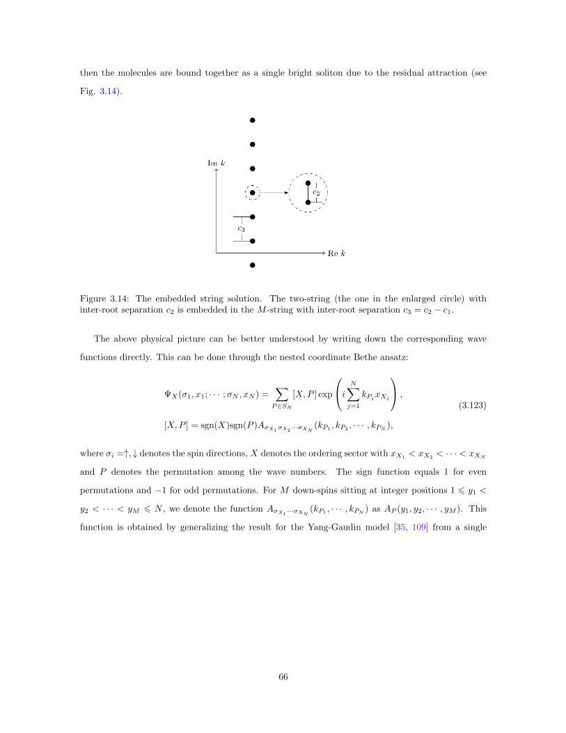
then the molecules are bound together as a single bright soliton due to the residual attraction (see

Fig. 3.14).

Figure 3.14: The embedded string solution. The two-string (the one in the enlarged circle) withinter-root separation c2 is embedded in the M -string with inter-root separation c3 = c2 − c1.

The above physical picture can be better understood by writing down the corresponding wave

functions directly. This can be done through the nested coordinate Bethe ansatz:

ΨX(σ1, x1; · · · ;σN , xN ) =∑P∈SN

[X,P ] exp

i N∑j=1

kPjxXj

,

[X,P ] = sgn(X)sgn(P )AσX1σX2···σXN (kP1 , kP2 , · · · , kPN ),

(3.123)

where σi =↑, ↓ denotes the spin directions, X denotes the ordering sector with xX1< xX2

< · · · < xXN

and P denotes the permutation among the wave numbers. The sign function equals 1 for even

permutations and −1 for odd permutations. For M down-spins sitting at integer positions 1 6 y1 <

y2 < · · · < yM 6 N , we denote the function AσX1···σXN (kP1

, · · · , kPN ) as AP (y1, y2, · · · , yM ). This

function is obtained by generalizing the result for the Yang-Gaudin model [35, 109] from a single

66

coupling constant cF to two coupling constants c1 and c2:

AP (y1, y2, · · · , yM ) =∑R∈SM

G1(P )G2(R)

M∏i=1

FP (yi,ΛRi),

G1(P ) =∏j<l

(kPj − kPl + ic1),

G2(R) = sgn(R)∏j<l

(ΛRj − ΛRl + ic2),

FP (y,Λ) =

y−1∏j=1

(kPj − Λ− ic′2)

N∏l=y+1

(kPl − Λ + ic′2).

(3.124)

For a concrete illustration, we substitute Eq. (3.122) into Eqs. (3.123) and (3.124) in the case with

N = 4, then in the basic sector I : x1 < x2 < x3 < x4, we have:

ΨI(↑, x1; ↓, x2; ↑, x3; ↓, x4) ∼ e−c′2(x2+x4−x1−x3)−c′3(x3+x4−x1−x2),

ΨI(↑, x1; ↑, x2; ↓, x3; ↓, x4) = 0,

ΨI(↑, x1; ↓, x2; ↓, x3; ↑, x4) ∼ e−c′2(x2+x4−x1−x3)−c′3(x3+x4−x1−x2),

(3.125)

where we have set u = 0 for simplicity. The expression for other ordering sectors then follows from the

symmetry of the system. Through the explicit wave function, the physical picture of the embedded

string solution is transparent, where the exponential decay on the length scale of 1/c′2 represents the

molecule structure and the exponential decay on the length scale of 1/c′3 binds all the M molecules

together.

3.5 Conclusion

In this chapter, we introduced models of two-component bosons and fermions with tunable inter-

species interactions in one dimension, where the Yang-Baxter equation for exact solvability can be

fulfilled by fine-tuning the model parameters. The tunable interactions are realized by Feshbach

resonances of two antiparallel pseudospins. The N atoms in this model can be imagined to live

on hyperplanes corresponding to different ordering sectors X : xX1< xX2

, < · · · < xXN . Without

reaction that converts atoms and molecules back and forth, we only need to require the continuity of

wave function when hyperplanes intersect. With Feshbach resonances, the molecules can be viewed as

living on the intersections of the hyperplanes, which play the role of the boundary conditions. Although

the strict exact solvability beyond the level of two-body scatterings would require the introduction

67

of extra singular counterterms, the present models can still be well described by the Bethe ansatz

for relatively small densities. The resulting Bethe ansatz equations admit two types of ground state

solutions, depending on the relation between the two coupling constants c1, c2. In the regime c1 > c2,

the ground state is a Fermi sea of two-strings, where the Fermi wave vector Q is under constraint:

there is a limiting Q∗ which Q cannot exceed, and near Q∗ the distribution of the center momentum

presents a square root singularity. As c2 approach c1 from below we come close to a diverging

compressibility, which leads us into the other regime c2 > c1 with a single N particle bound state for

the ground state. In the Bethe ansatz approach, this bound state reveals itself as an embedded string

solution. Our model is experimentally accessible by using two hyperfine states of 87Rb quantum gases

with tunable couplings via Feshbach resonance. Furthermore, the uniform regime c1 > c2 provides

a new scenario for investigating the physics of BCS-BEC crossover, where the system is governed by

a single Hamiltonian and the behavior of the spin excitations is accessible along the whole range of

the crossover. Also, we have explored the zero temperature phase diagram in presence of external

magnetic field, where a critical magnetic field below which the ground state cannot be polarized is

caused by the presence of the upper bound Q∗ for the Fermi momentum.

68

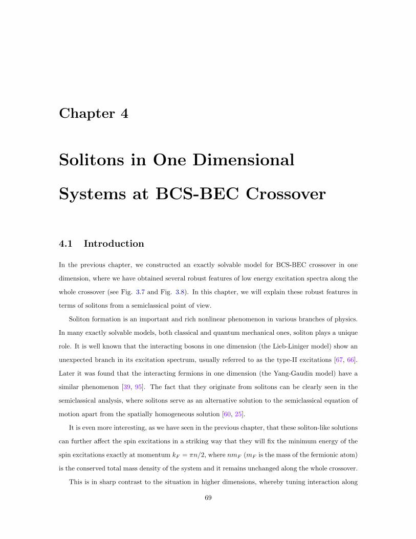
Chapter 4

Solitons in One Dimensional

Systems at BCS-BEC Crossover

4.1 Introduction

In the previous chapter, we constructed an exactly solvable model for BCS-BEC crossover in one

dimension, where we have obtained several robust features of low energy excitation spectra along the

whole crossover (see Fig. 3.7 and Fig. 3.8). In this chapter, we will explain these robust features in

terms of solitons from a semiclassical point of view.

Soliton formation is an important and rich nonlinear phenomenon in various branches of physics.

In many exactly solvable models, both classical and quantum mechanical ones, soliton plays a unique

role. It is well known that the interacting bosons in one dimension (the Lieb-Liniger model) show an

unexpected branch in its excitation spectrum, usually referred to as the type-II excitations [67, 66].

Later it was found that the interacting fermions in one dimension (the Yang-Gaudin model) have a

similar phenomenon [39, 95]. The fact that they originate from solitons can be clearly seen in the

semiclassical analysis, where solitons serve as an alternative solution to the semiclassical equation of

motion apart from the spatially homogeneous solution [60, 25].

It is even more interesting, as we have seen in the previous chapter, that these soliton-like solutions

can further affect the spin excitations in a striking way that they will fix the minimum energy of the

spin excitations exactly at momentum kF = πn/2, where nmF (mF is the mass of the fermionic atom)

is the conserved total mass density of the system and it remains unchanged along the whole crossover.

This is in sharp contrast to the situation in higher dimensions, whereby tuning interaction along

69

the BCS-BEC crossover we can move this momentum from kF on the deep BCS side to zero on the

deep BEC side [76]. In this chapter, we present a comprehensive semiclassical theory of solitons in

one dimensional systems at BCS-BEC crossover, where we explain the soliton interpretation of the

type-II excitations and the fixing of the momentum for the minimum energy of spin excitations. Our

theory gives the semiclassical interpretation of the excitation spectrum of the Yang-Gaudin model,

where existing semiclassical proposals fail to reconcile with the exact solutions [25, 95]. Our theory

also serves as yet another example of the dramatic effect solitons can have on low dimensional physics.

In the next section, we will review the exact solutions of the Lieb-Linger model, the Yang-Gaudin

model and the model of BCS-BEC crossover in one dimension. We then further analyze them in the

sections to follow. We first outline the general formalism of the semiclassical analysis in presence of

solitons across the BCS-BEC crossover. We then apply it to the S = 1/2 and S = 0 excitations

respectively, where we present analytic analysis on both deep BCS and deep BEC side and qualitative

analysis for the crossover. Finally, we summarize the main results and make the conclusion.

4.2 Review of Exact Solutions and their Relation to Solitons

In Sec. 3.2.1, we have reviewed the Lieb-Liniger model for interacting bosons and the Yang-Gaudin

model for interacting fermions, and we have constructed the exactly solvable models for BCS-BEC

crossover in one dimension. The low energy excitation spectra for the latter are worked out in Sec.

3.3.2. In this section, we summarize the excitation spectra of these exactly solvable models. In

the gapless S = 0 excitations spectrum (where S is the total spin) for all these models, there is

an extra soliton-like branch apart from the usual Bogoliubov quasiparticle branch. In the gapped

S = 1/2 excitations, one finds the minimum of the energy lying exactly at the Fermi momentum kF =

πn/2. These are the key features we would like to explain when later developing the corresponding

semiclassical theory.

We start with the Lieb-Liniger model, described by the Hamiltonian in Eq. (3.2):

H =

∫dx[∂xϕ

†(x)∂xϕ(x) + cBϕ†(x)ϕ†(x)ϕ(x)ϕ(x)

], (4.1)

where ϕ represents the spinless bosons with mass mB = 1/2, and cB > 0 corresponds to the repulsion

between bosons. A typical excitation spectrum of Lieb-Liniger model is shown in Fig. 4.1. It is

composed of two branches, the usual Bogoliubov quasiparticle (Lieb-Liniger type-I) branch, and the

Lieb-Liniger type-II branch. At long wavelength, both branches reduce to a linear dispersion as

70

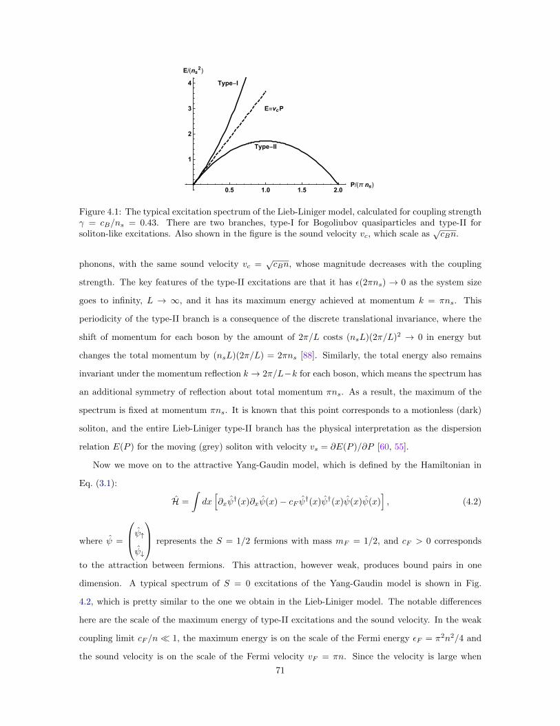
Type-I

Type-II

E=vcP

0.5 1.0 1.5 2.0P/(π ns)

1

2

3

4

E/(ns2)

Figure 4.1: The typical excitation spectrum of the Lieb-Liniger model, calculated for coupling strengthγ = cB/ns = 0.43. There are two branches, type-I for Bogoliubov quasiparticles and type-II forsoliton-like excitations. Also shown in the figure is the sound velocity vc, which scale as

√cBn.

phonons, with the same sound velocity vc =√cBn, whose magnitude decreases with the coupling

strength. The key features of the type-II excitations are that it has ε(2πns) → 0 as the system size

goes to infinity, L → ∞, and it has its maximum energy achieved at momentum k = πns. This

periodicity of the type-II branch is a consequence of the discrete translational invariance, where the

shift of momentum for each boson by the amount of 2π/L costs (nsL)(2π/L)2 → 0 in energy but

changes the total momentum by (nsL)(2π/L) = 2πns [88]. Similarly, the total energy also remains

invariant under the momentum reflection k → 2π/L−k for each boson, which means the spectrum has

an additional symmetry of reflection about total momentum πns. As a result, the maximum of the

spectrum is fixed at momentum πns. It is known that this point corresponds to a motionless (dark)

soliton, and the entire Lieb-Liniger type-II branch has the physical interpretation as the dispersion

relation E(P ) for the moving (grey) soliton with velocity vs = ∂E(P )/∂P [60, 55].

Now we move on to the attractive Yang-Gaudin model, which is defined by the Hamiltonian in

Eq. (3.1):

H =

∫dx[∂xψ

†(x)∂xψ(x)− cF ψ†(x)ψ†(x)ψ(x)ψ(x)], (4.2)

where ψ =

ψ↑ψ↓

represents the S = 1/2 fermions with mass mF = 1/2, and cF > 0 corresponds

to the attraction between fermions. This attraction, however weak, produces bound pairs in one

dimension. A typical spectrum of S = 0 excitations of the Yang-Gaudin model is shown in Fig.

4.2, which is pretty similar to the one we obtain in the Lieb-Liniger model. The notable differences

here are the scale of the maximum energy of type-II excitations and the sound velocity. In the weak

coupling limit cF /n 1, the maximum energy is on the scale of the Fermi energy εF = π2n2/4 and

the sound velocity is on the scale of the Fermi velocity vF = πn. Since the velocity is large when

71

Type-I

Type-II

E=vcP,vc∼vF

ϵF

0.5 1.0 1.5 2.02P/(π n)

1

2

3

4

5

E/(n2)

Figure 4.2: The typical S = 0 excitation spectrum of the Yang-Gaudin model, calculated for couplingstrength γ = cF /n = 0.15. There are also two branches, type-I for Bogoliubov quasiparticles andtype-II for soliton-like excitations. Also shown in the figure is the sound velocity and the Fermienergy εF , we can see in the weak coupling limit, the dark soliton has an energy on the scale of εFand the sound velocity is on the scale of vF .

k → 0, there is no semiclassical description for the dispersion relation, but near the maximum of the

spectrum where the velocity is small, a semiclassical description is still possible. The recent attempt

by [25] to develop such a description led to incorrect energy scale and curvature near the maximum

of the spectrum [95]. We are going to reconcile this discrepancy in this chapter.

In the strong coupling limit cF /n 1 where the fermions are tightly bound, instead of behaving

like a system of weakly coupled bosons, the Yang-Gaudin model produces a system of hardcore bosons

know as the fermionic super Tonks-Girardeau gas [39]. As a result, the sound velocity is still on the

scale of the Fermi velocity, and the spectrum of Fig. 4.2 preserves qualitative shape for any value of

cF .

A typical spectrum of S = 1/2 excitations of the Yang-Gaudin model is shown in Fig. 4.3,

where the minimum energy is achieved exactly at the Fermi momentum kF = πn/2, irrespective of

the coupling strength. This exactness is unusual, since it is without the correction on the scale of

δk ∼ ∆0/vF that would be introduced by the conventional BCS theory in the weak coupling limit

(where ∆0 is the gap width), and it is contrary to the usual conclusion that the minimum energy

should be achieved at zero momentum in deep BEC regime in higher dimensions [76]. At first sight,

this could be caused by the fact that the strong coupling limit cF /n 1 of Yang-Gaudin model is not

a system of weakly coupled bosons, which invalidates it as a proper model for BCS-BEC crossover.

To test this idea, our models proposed in the previous chapter come into play. The fermionic version

72

Pmin=kF=π n

2

ϵb

0.8 0.9 1.0 1.1 1.22P/(π n)

0.2

0.4

0.6

0.8

1.0

E/n2

Figure 4.3: The typical S = 1/2 excitation spectrum of the Yang-Gaudin model, calculated forcoupling strength γ = cF /n = 1.13. The minimum energy is obtained at the Fermi momentumkF = πn/2, with a small region of quadratic spectrum around it. Also shown in the figure is thebinding energy εb for the singlet pairs, which is bigger than the spin gap.

is described by the Hamiltonian in Eq. (3.7):

H =

∫dx

∂xψ

†∂xψ +1

2∂xΞ

† · ∂xΞ +1

2∂xΠ†∂xΠ− εΠΠ†Π + gψ†ψ†ψψ

+

[tΞ2

(i∂xψ

Tσσyψ)· Ξ† + h.c.

]+

[tΠ2

(iψTσyψ

)· Π† + h.c.

],

(4.3)

where ψ =

ψ↑ψ↓

represents the spin-1/2 fermions with mass mF = 1/2, Ξ represents the vector

resonances with binding energy εΞ and Π represents the scalar resonances with binding energy εΠ.

Both resonances are of mass mΞ = mΠ = 1. The behavior of this model is then controlled by two

parameters:

c1 = |tΞ|2/4, c2 = c1 + |tΠ|2/(2εΠ). (4.4)

This model has the Lieb-Liniger model and the Yang-Gaudin model as its two limits in the parameter

range c1 ∼ c2 and c1 c2 respectively, thus providing a model of BCS-BEC crossover in one dimension

that is subject to exact solutions. On the side where it reduces to the Yang-Gaudin model with cF = c2,

the excitation spectrum is basically the same as shown in Fig. 4.2 and Fig. 4.3; On the side where

it reduces to the Lieb-Liniger model with cB = c1 − c2, the S = 0 spectrum is basically the same as

shown in Fig. 4.1. In addition to that, we also have S = 1/2 excitations now, whose typical behavior

is shown in Fig. 4.4. We can see that the spectrum has the same feature as that on the BCS side,

with the minimum energy still obtained exactly at the Fermi momentum kF = πn/2. even though

the S = 0 sector corresponds to weakly interacting bosons with vc vF .

In all the exactly solvable models presented above, the fixing of minimum spin excitation energy

at kF is a phenomenon robust against variations of coupling constants across the whole range, which

73

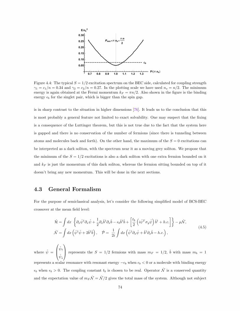
Pmin=π ns=π n

2

ϵb

0.7 0.8 0.9 1.0 1.1 1.2 1.3P/(π ns)

0.05

0.10

0.15

0.20

0.25

0.30

E/ns2

Figure 4.4: The typical S = 1/2 excitation spectrum on the BEC side, calculated for coupling strengthγ1 = c1/n = 0.34 and γ2 = c2/n = 0.27. In the plotting scale we have used ns = n/2. The minimumenergy is again obtained at the Fermi momentum kF = πn/2. Also shown in the figure is the bindingenergy εb for the singlet pair, which is bigger than the spin gap.

is in sharp contrast to the situation in higher dimensions [76]. It leads us to the conclusion that this

is most probably a general feature not limited to exact solvability. One may suspect that the fixing

is a consequence of the Luttinger theorem, but this is not true due to the fact that the system here

is gapped and there is no conservation of the number of fermions (since there is tunneling between

atoms and molecules back and forth). On the other hand, the maximum of the S = 0 excitations can

be interpreted as a dark soliton, with the spectrum near it as a moving grey soliton. We propose that

the minimum of the S = 1/2 excitations is also a dark soliton with one extra fermion bounded on it

and kF is just the momentum of this dark soliton, whereas the fermion sitting bounded on top of it

doesn’t bring any new momentum. This will be done in the next sections.

4.3 General Formalism

For the purpose of semiclassical analysis, let’s consider the following simplified model of BCS-BEC

crossover at the mean field level:

H =

∫dx

∂xψ

†∂xψ +1

2∂xb†∂xb− εbb†b+

[tb2

(iψTσyψ

)b† + h.c.

]− µN ,

N =

∫dx(ψ†ψ + 2b†b

), P =

1

2i

∫dx(ψ†∂xψ + b†∂xb− h.c.

),

(4.5)

where ψ =

ψ↑ψ↓

represents the S = 1/2 fermions with mass mF = 1/2, b with mass mb = 1

represents a scalar resonance with resonant energy −εb when εb < 0 or a molecule with binding energy

εb when εb > 0. The coupling constant tb is chosen to be real. Operator N is a conserved quantity

and the expectation value of mF N = N/2 gives the total mass of the system. Although not subject

74

to exact solutions, this model grasps the essence of the BCS-BEC crossover and is more friendly to

semiclassical analysis.

A conventional way to analyze the semiclassical origin of the excitations is to treat the operators as

classical fields and to solve the semiclassical equations of motion for them. Its validity can be justified

in the narrow resonance limit and via the saddle point approximation in the path integral formalism.

The symmetry-broken ground state of the system is then represented by the expectation value⟨b⟩

=

b0, where b0 is a constant, and the excitations are represented by a space-time varying expectation

value b(x, t) ≡⟨b⟩

, where we use the periodic boundary condition such that b(x, t) = b(x+ L, t). As

we treat the operator b as a classical field b(x, t), the part of H that involves fermionic operators can

be diagonalized via the Bogoliubov-Valatin transformation

ψ↑ψ†↓

=∑n

un(x, t) −v∗n(x, t)

vn(x, t) u∗n(x, t)

γn↑γ†n↓

(4.6)

to the following Hamiltonian

Hψ =∑εn>0

[−εn(∆,∆∗) + εn

∣∣∣tb=0

]+∑

εn>0,σ

εnγ†nσγnσ, (4.7)

where we have defined ∆(x, t) ≡ tbb(x, t) and the classical fields un(x, t), vn(x, t) satisfy the Bogoliubov-

de Gennes equation [94] with periodic boundary conditions:

−∂2x − µ ∆

∆∗ ∂2x + µ

unvn

= εn

unvn

,

un(x+ L, t) = un(x, t)

vn(x+ L, t) = vn(x, t)

.

(4.8)

Using these classical fields b(x, t), un(x, t) and vn(x, t), the energy and momentum of the system under

a particular filling configuration of Eq. (4.7) can then be expressed as

E =

∫dx

(1

2|∂xb|2 − (2µ+ εb)|b|2

)+ Eψ,

Eψ =∑εn>0

[−εn(∆,∆∗) + εn

∣∣∣tb=0

]+∑

εn>0,σ

εn⟨γ†nσγnσ

⟩,

P =

∫dx

(∑εn>0

u∗n←→∂xun + v∗n

←→∂xvn

2i

∑σ

⟨γ†nσγnσ

⟩)+

∫dx

(∑εn>0

(−i)vn←→∂xv

∗n +

b∗←→∂x b

2i

),

(4.9)

75

where Eψ is the eigenvalue of the mean field Hamiltonian Hψ in Eq. (4.7) under this particular filling

configuration, and the double arrow derivative is defined as

f←→∂x g ≡ f(∂xg)− (∂xf)g. (4.10)

The solutions to Eq. (4.8) have a special particle-hole symmetry that if (un, vn)T is a solution

with eigenvalue εn, then (−v∗n, u∗n)T must be a solution with eigenvalue −εn. As a result, nonzero

eigenvalues appear in pairs. Moreover, if Eq. (4.8) possesses zero eigenvalue, it must be degenerate,

otherwise we would have u0

v0

= c

−v∗0u∗0

, (4.11)

where (u0, v0)T is the solution to Eq. (4.8) for ε = 0 and c is constant complex number of modulus one

|c| = 1. Equation (4.11) would then lead to |c|2u0 = −u0, which cannot be true unless u0 is trivially

zero (This argument is analogous to that for Kramers degeneracy). In later sections where ∆(x, t) is

identified as a soliton, we find that the degenerate zero modes appear only in the deep BCS limit,

where the spectrum is linearized around the Fermi points. But this turns out to be an artifact of the

linearization, and there will be no zero mode when the nonlinear effect of the spectrum is taken into

account.

It is clear from the above analysis that the solutions to Eq. (4.8) always appear in pairs, the state

S = 0 then corresponds to a zero (or even) occupation of Bogoliubov fermions γnσ and the state

S = 1/2 is made out of odd occupation. Also as we will see in later sections, the state of the S = 0

soliton corresponding to the exact solution is not necessarily a ground state of Hψ.

4.3.1 Dark Soliton

The dark soliton is characterized by a twist in the configuration of b(x) where its value changes sign

rapidly from x < 0 to x > 0. Taking into consideration the periodic boundary condition, b(x) then

has the following asymptotic behavior at spatial boundaries:

b(x→ ±L/2) ∼ eiπx/L, (4.12)

where we are taking the infinite system limit that L→∞. It would be helpful to perform the following

gauge transformation:

b(x) = eiπx/Lb(x), (4.13)

76

then the dark soliton can be presented as

b(x) = −ib0f(x

ls

), (4.14)

where ls L is the size of the soliton sitting at x = 0, the constant number b0 is chosen to be real,

and the shape function f(x) has the asymptotic behavior that f(x → ±∞) = ±1. Under this gauge

transformation, the periodic boundary condition of b(x) becomes b(x+L) = −b(x). As a result, b(x)

can be chosen purely imaginary, or equivalently, f(x) can be chosen purely real.

To get rid of the phase in Eq. (4.13), we perform the following gauge transformation on the classical

fields un(x), vn(x): un(x) = eiπx/Lu(x)

vn(x) = vn

, (4.15)

then Eq. (4.8) is transformed into

−∂2x − µ tbb

(tbb)∗ ∂2

x + µ

unvn

= εn

unvn

,

un(x+ L, t) = −un(x, t)

vn(x+ L, t) = vn(x, t)

, (4.16)

where we have neglected both L−1 and L−2 correction to the eigenenergy εn. The former can be

neglected because it contributes to the total energy in Eq. (4.9) a term proportional to P/L, which

goes to zero in the limit L → ∞ for finite momentum P . The latter can be neglected because it

contributes to the total energy a term proportional to NL−2, which also goes to zero in the limit

L → ∞. Using these gauge transformed classical fields, the energy E, the momentum P and the

conserved quantity N of the system can be expressed as:

E =

∫dx

(1

2|∂xb|2 − (2µ+ εb)|b|2

)+ Eψ,

P =

∫dx

(∑εn>0

u∗n←→∂x un + v∗n

←→∂x vn

2i

∑σ

⟨γ†nσγnσ

⟩)+

∫dx

(∑εn>0

(−i)vn←→∂x v

∗n +

b∗←→∂x b

2i

)+N

2Lπ,

N =

∫dx∑εn>0

[(u∗nun − v∗nvn)

∑σ

⟨γ†nσγnσ

⟩]+

∫dx

(∑εn>0

2v∗nvn + 2b∗b

),

(4.17)

where the effect of gauge transformation is taken into account in the limit L→∞. The contribution

to the energy is vanishingly small (∼ NL−2) while the contribution to the momentum remains finite,

which appears in the expression for P as the last term proportional to n = N/L.

77

To be consistent with the choice that b(x) is purely imaginary, un(x) and vn(x) can be chosen purely

real and purely imaginary respectively. Since the classical fields b(x), un(x) and vn(x) are chosen to

be either purely real or purely imaginary, the contribution from the integral for the momentum P in

Eq. (4.17) is zero, then we arrive at the result that the momentum of the dark soliton is exactly the

Fermi momentum:

P = kF = πn/2, (4.18)

whether it is for a S = 0 state or a S = 1/2 state.

Now we have to determine the actual form of the dark soliton profile f(x). It is obtained by solving

the equation of motion for the classical field b(x). Because the dark soliton corresponds to a local

minimum or a local maximum of the energy for S = 0 or S = 1/2 spectrum respectively, the desired

equation of motion for b(x) can be derived by extremizing the energy E in Eq. (4.17):

− 1

2∂2xb− (2µ+ εb) b+

δEψ

δb∗= 0. (4.19)

Together with Eq. (4.16), we now have a complete set of equations to determine all the relevant

classical fields.

As mentioned at the end of Sec. 4.2, our proposal for S = 1/2 excitations is based upon the

assumption that one extra fermion can be bounded on the dark soliton, which is equivalent to the

assumption that there is at least one localized state solution to Eq. (4.16), so we present below a

simple one-parameter variational approach to verify this assumption.

The Hamiltonian operator corresponding to Eq. (4.16) is as follows:

Hb =

−∂2x − µ tbb

(tbb)∗ ∂2

x + µ

, (4.20)

and it has a positive as well as a negative sector, due to the particle-hole symmetry discussed after

Eq. (4.8). Accordingly, the existence of the localized state can be proved by the fact that the ex-

pectation value I(κ) of H2b on a normalized trial wave function ψκ(x) is below the boundary of the

continuous spectrum for H2b , where κ is the variational parameter:

I(κ) =

∫dx (Hψκ(x))

∗Hψκ(x),

∫dx ψ∗κ(x)ψκ(x) = 1. (4.21)

Here we make the choice that I(0) corresponds to the boundary of the continuous spectrum and κ > 0

78

corresponds to the localized state. Then the existence of localized state corresponds to I ′(0) < 0.

For µ > 0, the boundary of the continuous spectrum for H2b is ∆2

0 = (tbb0)2, and the normalized

trial wave function can be chosen as

ψκ =√κe−κ|x|

cos kFx

sin kFx

, (4.22)

where k2F = µ. Then we have

I(κ) = ∆20 + κ4 + 4κ2k2

F −∆20κls

∫e−2κls|y|f2(y)dy, (4.23)

which has the required property that

I(0) = ∆20, I ′(0) < 0. (4.24)

For µ 6 0, the boundary of the continuous spectrum for H2b is ∆2

0 + µ2, and the following normalized

trial wave function is chosen:

ψκ =√κe−κ|x|

1

0

, (4.25)

Then we have

I(κ) = (−κ2+ |µ|)2 + ∆20 −∆2

0κls

∫e−2κls|y|f2(y)dy, (4.26)

which again has the required property that

I(0) = ∆20 + µ2, I ′(0) < 0. (4.27)

Taking also into consideration that the solutions to Eq. (4.16) always appear in pairs and belong to

the negative and positive sectors respectively, we then proved here that there is at least one localized

state for each sector for the whole range of µ across the BCS-BEC crossover.

In later sections, we will show that the number of localized states is exactly one for each sector in

both the deep BCS and the deep BEC limit, and we didn’t find any evidence for the existence of a

second localized state (though appearance of such state would not violate any further consideration).

79

4.3.2 Grey Soliton

In order to transform the dark soliton into a moving grey soliton, we need to generalize the above

construction to the following asymptotic behavior at spatial boundaries:

b(x→ ±L/2, t) ∼ eiθsx/L, (4.28)

where the phase parameter θs ∈ [0, 2π) and we take the limit L→∞. We will show in later sections

that the moving grey soliton can be presented in the following form:

b(x, t) = b0

[cos

θs2− i sin

θs2f

(x− vstls

)]eiθsx/L, (4.29)

where vs is the velocity of the grey soliton. The velocity vs and phase parameter θs are not independent

variational variables. As we will show now, they are related to each other via the semiclassical velocity

formula vs = ∂E(θs)/∂P (θs).

Considering the transformation of the variables from (x, t) to (z, t) such that z = x− vst, we will

have

H → Ω = H+ivs2

∫dz(ψ†←→∂z ψ + b†

←→∂z b),

P → P =(−i)

2

∫dz(ψ†←→∂z ψ + b†

←→∂z b),

(4.30)

where we have variable x on the lefthand side and variable z on the righthand side. We can see

that in Eq. (4.30) new terms are added to the Hamiltonian operator, while the momentum operator

remains unchanged. This implies that the variable transformation introduced here is not a Galilean

transformation, for which the momentum would have been changed by the amount proportional to

vsN →∞. From Eq. (4.30) we obtain the following operator relations:

∂Ω

∂vs= −P, Ω = H − vsP. (4.31)

By taking the expectation values of both sides on the soliton with phase parameter θs, we can see

that the change of variables from x to z is equivalent to a Legendre transformation:

∂Ω(θs)

∂vs= −P (θs), Ω(θs) = E(θs)− vsP (θs). (4.32)

80

By taking derivative with respect to θs of both sides of the second equation in (4.32), we obtain

∂Ω

∂θs=∂E

∂θs− ∂vs∂θs

P − vs∂P

∂θs. (4.33)

Then using the first equation in (4.32) we also obtain

∂Ω

∂θs=∂Ω

∂vs

∂vs∂θs

= −∂vs∂θs

P. (4.34)

Combining Eq. (4.33) and Eq. (4.34), we arrive at the following equation

vs =∂E/∂θs∂P/∂θs

=∂E

∂P. (4.35)

When the soliton is interpreted as a proper excitation, Eq. (4.35) is just the semiclassical velocity

formula mentioned above, which determines the soliton velocity vs as a function of θs. Then the fact

that the dark soliton corresponds to either the maximum (S = 0) or minimum energy (S = 1/2)

follows from the condition that vs(θs = π) = 0.

As in derivation for the dark soliton, it would be helpful to do the following gauge transformation

of the classical fields: b(x, t) = ei

θsxL b(z),

un(x, t) = eiθsxL un(z),

vn(x, t) = vn(z),

(4.36)

where z = x − vst. This leaves us with the analysis of classical fields b(z) or ∆(z) = tbb(z), un(z)

and vn(z), for which we will omit the tilde in the following whenever there is no confusion. Also, the

gauge transformation modifies the boundary conditions of the classical fields:

b(z + L) = e−iθsb(z),

un(z + L) = e−iθsun(z),

vn(z + L) = vn(z).

(4.37)

Using these classical fields, again we can write down the expressions for the energy E, momentum P

81

and the conserved quantity N :

E =

∫dz

(1

2|∂zb|2 − (2µ+ εb)|b|2

)+ Eψ,

P =

∫dz

(∑εn>0

u∗n←→∂z un + v∗n

←→∂z vn

2i

∑σ

⟨γ†nσγnσ

⟩)+

∫dz

(∑εn>0

(−i)vn←→∂z v

∗n +

b∗←→∂z b

2i

)+N

2Lθs,

N =

∫dz∑εn>0

[(u∗nun − v∗nvn)

∑σ

⟨γ†nσγnσ

⟩]+

∫dz

(∑εn>0

2v∗nvn + 2b∗b

),

(4.38)

where the energy and momentum are understood by taking the reference point that E(θs = 0) = 0

and P (θs = 0) = 0. Also, the chemical potential is determined by the usual thermodynamic relation

that µ = ∂E/∂N .

For a particular filling configuration of the mean field Hamiltonian Hψ in Eq. (4.7), we now derive

the semiclassical equations of motion for the classical fields b(z), un(z) and vn(z). Unlike the dark

soliton, the grey soliton only extremizes the energy E under certain constraints. Usually we would

extremize the energy E under the constraint of fixed momentum P , but this approach may not

respect the desired boundary condition in Eq. (4.37). To overcome this difficulty, we use a modified

extremization process. Firstly, we partition the momentum P in Eq. (4.38) into two parts: the

contribution Pψ from the fermion fields and the contribution Pb from the b field:

Pb =

∫dz

((−i)

2b∗←→∂z b+

b∗bLθs

), Pψ = P − Pb (4.39)

Then instead of keeping P fixed, we keep both Pψ and Pb fixed, and this introduces two Lagrangian

multiplier vψ and vb into the free energy F we want to extremize:

E → F = E − vψPψ − vbPb. (4.40)

We can visualize this modified extremization in the functional space spanned by Pψ and Pb (see Fig.

4.5). Each point on the hyperline Pψ + Pb = P corresponds to an extreme of the free energy F ,

and one point among them (the starred point in Fig. 4.5) is picked out by adjusting the Lagrangian

multiplier pair (vψ, vb) to satisfy the boundary condition in Eq. (4.37). This modified extremization

process is morally equivalent to the method of constrained instanton used in field theories [2]. Also,

82

following the derivation from Eq. (4.32) to Eq. (4.35), we obtain

dE = vψdPψ + vbdPb = vs(dPψ + dPb). (4.41)

This allows a trivial solution that vψ = vb = vs or a nontrivial solution such that

vs − vψvb − vs

=∂Pb∂Pψ

. (4.42)

We will see in later sections that the nontrivial solution is crucial on the deep BCS side.

Figure 4.5: The functional space for the extremization spanned by Pψ and Pb. The thick line isthe collection of extreme points and the starred point is the one that satisfies the required boundarycondition in Eq. (4.37).

Applying the modified extremization process, we obtain the following equations of motion for the

classical fields in the limit L→∞:

− 1

2∂2zb+ ivb∂zb− (2µ+ εb) b+

δEψδb∗

= 0, (4.43)

−∂2z − µ+ ivψ∂z ∆(z)

∆∗(z) ∂2z + µ+ ivψ∂z

unvn

= εn

unvn

, (4.44)

where ∆(z) field is related to b(z) field through the definition ∆(z) = tbb(z) and the eigenvalue εn

differs from εn in Eq. (4.7) and Eq. (4.8) in that εn contributes to the free energy F in Eq. (4.40)

while εn contributes to the energy E in Eq. (4.9). We should keep this in mind when later calculating

the energy E. Also, the proof of the existence of the localized state for a dark soliton can be easily

generalized here to Eq. (4.44) for a grey soliton.

83

4.4 Theory of S = 1/2 Soliton

In this section, we apply the general formalism outlined above to the S = 1/2 soliton, which turns

out to be simpler than the S = 0 soliton. The two weak coupling limits - the deep BCS side and the

deep BEC side - permit analytical treatment, because on either side, one of the degrees of freedom

lies high in energy compared to the other such that we are left with a decoupled theory with weak

interaction.

4.4.1 Deep BCS Side

On the deep BCS side, we tune the resonant level of b field far above the Fermi sea such that

εb < 0, |εb| µ. Since the b field now only acts as a virtual state to effect the low energy physics, we

can ignore its dynamics, and the equation of motion for it reduces to a self-consistent equation:

∆ = λ∑εn>0

unv∗n

(1−

∑σ

⟨γ†nσγnσ

⟩)+ τ(i∂z∆), (4.45)

where λ = |tb|2−(2µ+εb)

> 0 serves as the effective coupling constant and τ = vb/(2µ + εb). Also for the

dark soliton, we should bear in mind that we need to set vψ = vb = 0 and τ = 0. Combined with the

equation of motion for the fermion fields, we can reconstruct the Hamiltonian as

H =

∫dz

(∑σ

ψ†σ(−∂2

z − µ)ψσ

)+

∫dz

(∆∗ψ↓ψ↑ + ∆ψ†↑ψ

†↓ +|∆|2λ

). (4.46)

This is just the BCS mean field Hamiltonian for the conventional superconductivity and the ∆ field

is just the gap parameter. Thus, our semiclassical analysis on the deep BCS side can be equally well

applied to the Yang-Gaudin model in the weak coupling limit. The system is made out of loosely

bounded Cooper pairs, and we have a large chemical potential µ = k2F , where kF = πn/2 and n = N/L.

Since the low energy physics happens only near the two Fermi points, we can linearize the spectrum

around them: unvn

=∑α

uαnvαn

eiαkF z, (4.47)

84

where α = −1 and α = 1 denotes the left and right moving modes respectively. Correspondingly,

Eq. (4.44) can be linearized to the following form:

−iαvF∂z − αvψkF ∆(z)

∆∗(z) iαvF∂z − αvψkF

uαnvαn

= εαn

uαnvαn

, (4.48)

where the bar notation of the eigenvalue again reminds us that εαn contributes to the free energy F

instead of the energy E. Moreover, due to the linearization made here, we can further determine the

eigenvalue εαn that contributes to energy E as εαn = εαn + αvψkF .

The solution to this linearized Bogoliubov-de Gennes equation under soliton profile in the context of

polyacetylene and charge density waves is well established in the literature [97, 100, 10, 11]. Essentially,

the solvability comes from the fact that Eq. (4.48) has the form of Dirac equation in one dimension

and it can be associated with a nonlinear Schrodinger equation for the ∆(z) field via the inverse

scattering method [30]. There then exists the following soliton solution:

∆(z) = ∆0

[cos

θs2− i sin

θs2

tanh

(z

ls

)], (4.49)

where the size of the soliton is l−1s =

(∆0 sin θs

2

)/vF . The eigenmodes of Eq. (4.48) can be classified

into two categories. The first category includes the delocalized states labelled by left-right moving

index α = ±, band index ι = ± and momentum k:

uαιk = 1

21√NαιkL

[1 + α

vF k+i∆2 tanh(

∆2vFz)

ειk−α∆1

]eikz

vαιk = 12

1√NαιkL

[−α+

vF k+i∆2 tanh(

∆2vFz)

ειk−α∆1

]eikz

,

∆1 = ∆0 cosθs2, ∆2 = ∆0 sin

θs2, Nα

ιk =ειk

ειk − α∆1.

(4.50)

The corresponding eigenvalues are

εαιk = ειk − αvψkF , ειk = ιεk, εk =√

∆20 + v2

F k2. (4.51)

so the band ι = + corresponds to the excitations defined in Eq. (4.7). The second category is the

localized states on the soliton core, labelled only by the left-right moving index α:

uα0vα0

=1

2

√∆2

vFsech

(∆2z

vF

)1

α

, (4.52)

85

and the corresponding eigenvalues are:

εα0 = εα0 − αvψkF , εα0 = α∆0 cosθs2. (4.53)

According to the above expression for the eigenvalues, the localized states corresponding to the dark

soliton (θs = π, vψ = 0) are degenerate zero modes, but this degeneracy is an artifact of the lineariza-

tion in Eq. (4.47), while the correction from the quadratic spectrum up to leading order will lift this

degeneracy:

εα0 = α

√∆2

0 −[∆0 sin

θs2− πvF kF

2csch

(πlskF

2

)]2

. (4.54)

The actual localized states are linear combinations of the left and right moving localized states, so the

superscript α = ± in Eq. (4.54) labels positive and negative modes instead of left and right moving

modes.

To complete the construction of the soliton, we still need to satisfy the self-consistent requirement

in Eq. (4.45). In the present classification of the eigenmodes, it is expressed as

∆ = λ∑α,k

uα+,kvα+,k∗(

1−∑σ

⟨γα†+,k,σγ

α+,k,σ

⟩)+ λu+

0 v+0

∗(

1−∑σ

⟨γ+†

0,σγ+0,σ

⟩)+ τ(i∂z∆). (4.55)

The S = 1/2 soliton is obtained by setting∑σ

⟨γα†+,k,σγ

α+,k,σ

⟩= 0 and

∑σ

⟨γ+†

0,σγ+0,σ

⟩= 1, then the

above equation reduces to

∆ = λ

∫dk

2π

∆

εk+λ

4

∆0

vF

θs − ππ

sin θs2

cosh2(

∆2

vFz) + τ(i∂z∆). (4.56)

For the dark soliton, the second part on the righthand side vanishes and we need to set τ = 0, then

the resulting equation is exactly the one we have in conventional BCS theory with a homogenous gap

parameter:

1 = λ

∫dk

2π

1

εk⇒ ∆0 ∝ exp

(− 1

λν(εF )

), (4.57)

where ν(εF ) is the density of states on the Fermi level.

For the moving grey soliton, the second part on the righthand side of Eq. (4.56) has a finite value,

but it can be canceled by the third term under the choice that

τ =λ

4∆0

π − θsπ

sin−1 θs2, (4.58)

86

Pmin=kF=π n

2

--: Exact

—: Semiclassic

0.98 0.99 1.00 1.01 1.02 1.032P/(π n)

0.05

0.10

0.15

0.20

E/n2

Figure 4.6: The typical S = 1/2 excitation spectrum in the semiclassical result and exact solution.The latter is plotted for γ = cF /n = 1.13, and correspondingly the former is plotted taking the spingap at the same coupling strength as the input parameter.

which then determines vb as

vb =|tb|24∆0

θs − ππ

sin−1 θs2. (4.59)

We can see that determination of parameters τ, vb in the above equation is consistent with τ = 0, vb = 0

for θs = π in the case of dark soliton.

Having specified the S = 1/2 soliton, we can proceed to calculate its energy and momentum near

the dark soliton up to leading order in ξ = θs − π using the formula in Eq. (4.38) and Eq. (4.7). The

calculation consists of first determining the phase shift δ(k) for the continuous spectrum from the

boundary conditions in Eq. (4.37) and then changing the summations over k into integrations while

taking into account the correction due to the phase shift δ(k) in the limit L→∞ [100, 25]. Also, we

need to keep in mind that we should use εαn instead of εαn in the calculation of energy E. The final

result is:

EBCS1/2 (θs) =

2∆0

π

(1 +

1

8ξ2

), PBCS

1/2 (θs) = kF −∆0

2vFξ. (4.60)

This translates into the following dispersion relation and soliton velocity up to leading order in ξ:

E1/2 =2∆0

π

(1 +

v2F (P1/2 − kF )2

2∆20

), vBCS

s =∂E1/2

∂P1/2= − ξ

πvF . (4.61)

It is clear that the minimum energy is achieved exactly at the Fermi momentum kF = πn/2, as

observed in the exact solutions. Also, the soliton velocity now is characterized by the Fermi velocity

vF , which is also consistent with the exact solutions. A comparison of the current semiclassical result

with the exact solution is shown in Fig. 4.6, where the agreement is good in the vicinity of the dark

soliton.

87

To complete the analysis, we still need to determine vψ and vb from Eq. (4.42). In order to do

that, we need the expressions for Pψ and Pb respectively:

Pb =∆2

0

|tb|2(π + 2ξ), Pψ = PBCS

1/2 (θs)− Pb. (4.62)

Substituting them into Eq. (4.42) and using Eq. (4.59), we obtain up to leading order:

vb =|tb|2

4π∆0ξ, vψ = vBCS

s − vBCSs − vb

1 + |tb|2/(4∆0vF )≈ vBCS

s , (4.63)

where the expression for vψ will be of use in later section when we analyze the S = 0 soliton. This

closes our analysis of the S = 1/2 soliton on the deep BCS side.

4.4.2 Deep BEC Side

On the BEC side, we tune the resonant level to a tightly bounded molecule with binding energy εb > 0.

Then we have a negative chemical potential µ < 0 characterizing the absence of a Fermi sea, and we

need to consider the quadratic Bogoliubov-de Gennes equation in Eq. (4.44). For delocalized states

characterized by momentum k, we formally obtain the spectrum of Bogoliubov quasiparticles as:

εk =√

(k2 − µ)2 + |∆|2. (4.64)

For large negative chemical potential µ, we can expand the spectrum as

εk = (k2 − µ) +|∆|2

2(k2 − µ)− |∆|4

8(k2 − µ)3+ · · · . (4.65)

Substituting this into Eq. (4.43), we can bring the equation of motion for b = ∆/tb to the following

form known as the Gross-Pitaevskii equation:

− 1

2∂2zb+ ivb∂zb+ 2g(|b|2 − ns)b = 0, (4.66)

where the parameters are defined via

g =3|tb|4

128|µ|5/2 , ns =

|tb|24|µ|1/2 + 2µ+ εb

3|tb|464|µ|5/2

. (4.67)

The Gross-Pitaevskii equation as a nonlinear Schrodinger equation has been extensively studied

88

Figure 4.7: The Feynman diagrams (left) for leading contribution to the scattering process ψb→ ψb(right), where the solid line denotes the fermion propagator, the wiggled line denotes the bosonpropagator, the fermion-boson vertex denotes the resonant coupling tb, and the dotted vertex on theright denotes the effective coupling g′.

in the literature [104, 111, 112, 60, 55]. It also supports a soliton solution:

b(z) =√ns

(cos

θs2− i sin

θs2

tanhz

ls

), (4.68)

where the size of the soliton is ls = [vc sin(θs/2)]−1, the Lagrangian multiplier is vb = vc cos(θs/2) and

vc =√gn is the sound velocity. By calculating the total mass of the system we can also determine

ns = n/2.

The S = 1/2 soliton is constructed by adding an extra fermion into the system, then we can

effectively describe the system as follows: There is a weakly interacting background (the bound pairs)

with the effective coupling constant g. The extra fermion added into the system interacts with the

background locally by an effective coupling constant g′, which can be calculated perturbatively from

Eq. (4.5) in the narrow resonance limit. For this purpose, we consider the scattering process ψb→ ψb,

whose Feynman diagrams are shown in Fig. 4.7. The scattering amplitude up to leading order is then

g′(ω, k) = − |tb|2

ω − εk≈ |tb|

2

−2µ> 0. (4.69)

As a result, the added fermion ψ can be described as a quantum particle moving in the potential

created by the background:

(−∂2z − µ+ ivψ∂z)ψ + g′(|b|2 − ns)ψ = εψ, (4.70)

where in the second term on the lefthand side, we have adjusted for the interaction of the fermion

with the uniform background (the constant term g′ns), since it can be incorporated into the chemical

89

potential. Performing the gauge transformation ψ → ψeivψz/2 which shifts the momentum by vψ/2,

and substituting Eq. (4.68) into Eq. (4.70), we end up with a Schrodinger equation for a particle

moving in the Poschl-Teller potential [84]:

− ∂2zψ − α2 ζ(ζ − 1)

cosh2 αzψ =

(ε+ µ+

v2ψ

4

)ψ, (4.71)

where the two parameter α and ζ > 1 are determined by

α = vc sin(θs/2), α2ζ(ζ − 1) = g′ns sin2(θs/2). (4.72)

The Poschl-Teller potential produces a bound state with the following energy:

ε0 = −α2(ζ − 1)2 −v2ψ

4− µ = −v2

c sin2 θ2

2

(√1 + 2g′/g − 1

2

)2

−v2ψ

4+ |µ|. (4.73)

Also the momentum of this bound state is simply k0 = vψ/2, and we can determine the eigenvalue ε0

that contributes to the energy E as

ε0 = ε0 + vψk0. (4.74)

Then the total energy E1/2(θs) and momentum P1/2(θs) of the system can be determined according

to Eq. (4.38):

EBEC1/2 (θs) =

∫dz

(1

2|∂zb|2 + g(|b|2 − ns)2

)+ ε0 = nsvc

[4

3sin3 θs

2− 2u sin2 θs

2

]+

1

4v2ψ + |µ|,

PBEC1/2 (θs) =

∫dz

1

2i(b∗∂zb− b∂zb∗) + nsθs + k0 = ns(θs − sin θs) +

1

2vψ,

(4.75)

where u =√

gn

(√1+2g′/g−1

2

)2

1 in the narrow resonance limit. Thus the minimum of EBEC1/2 (θs)

is at θs = π with the following minimum energy:

EBEC1/2 (θs = π)− |µ| = nsvc

(4

3− 2u

)< 0, (4.76)

so EBEC1/2 (θs = π) is lower than the energy of adding one particle with zero momentum to the uniform

background of bound pairs. Again, we arrive at the conclusion that the minimum energy is achieved

exactly at the Fermi momentum kF = πns = πn/2.

We are then left with the determination of the velocities vψ, vs in addition to vb = vc cos(θs/2),

90

Pmin=π ns=π n

2

--: Exact

—: Semiclassic

0.94 0.96 0.98 1.00 1.02 1.04 1.06P/(π ns)

0.170

0.175

0.180

0.185

0.190

E/(ns2)

Figure 4.8: The typical S = 1/2 excitation spectrum in the semiclassical result and the exact solution.The former is plotted for γ = g/n = 0.07, and correspondingly the latter is plotted for δγ = γ1−γ2 =0.07.

which should be obtained by solving Eq. (4.41). Here the trivial solution will do the work:

vψ = vb = vBECs = vc cos

θs2. (4.77)

A comparison of the current semiclassical result and the exact solution is shown in Fig. 4.8, they

agree well in the vicinity of P = kF .

In between the deep BCS and BEC sides, the physical picture of the S = 1/2 excitations remain

the same - they are moving solitons with one extra fermion bounded on the soliton core (see Fig.

4.9). This explains what we observed in exact solutions: instead of adding one particle on the uniform

background, the more energy-favorable excitation is the addition of one particle on the dark soliton.

The energy cost in the creation of the dark soliton is offset by the energy gain of trapping the particle

inside the dip of the density profile. The fact that the minimum energy is achieved exactly at the

Fermi momentum is then a consequence of the soliton formation.

Figure 4.9: The physical picture of the S = 1/2 excitations along the BCS-BEC crossover - they areone extra spin trapped in the density dip produced by the dark or grey soliton configuration.

4.5 Theory of S = 0 Soliton

In this section, we apply the general formalism to the S = 0 soliton, where we will find a crossover

between the two weak coupling limits of the soliton structure.

91

4.5.1 Deep BEC Side

The analysis on the deep BEC side is simpler, since we have only the Gross-Pitaevskii equation for

the classic field b(z) presented in Eq. (4.66), and we don’t need to worry about the self-consistency

requirement as in Eq. (4.45). In fact, from Eq. (4.66) we can reconstruct the low energy effective

Hamiltonian as

H =

∫dz

[1

2∂z b†∂z b+ gb†b†bb

], (4.78)

with is just the Lieb-Liniger model defined in Eq. (3.2) but with the mass mb = 1. As mentioned

previously, the fact that S = 0 (type-II) excitations of the Lieb-Liniger model have the physical

interpretation as moving solitons is well understood [60, 55]. The energy and momentum can be

calculated directly using the soliton profile in Eq. (4.68):

EBEC0 (θs) =

∫dz

(1

2|∂zb|2 + g(|b|2 − ns)2

)=

4

3nsvc sin3 θs

2

PBEC0 (θs) =

∫dz

1

2i(b∗∂zb− b∂zb∗) + nsθs = ns(θs − sin θs),

(4.79)

then the soliton velocity is determined as vBECs = ∂E0/∂P0 = vc cos(θs/2), which is consistent with

the result in Eq. (4.77). A comparison of the semiclassical result with the exact solution is shown in

Fig. 4.10, where in the weak coupling limit, we will obtain a next to perfect match [60].

--: Exact

—: Semiclassic

E=vcP

0.5 1.0 1.5 2.0P/(π ns)

0.5

1.0

1.5

2.0

E/(ns2)

Figure 4.10: The typical S = 0 excitation spectrum in the semiclassical result and the exact solution,The former is plotted for γ = g/n = 0.06, and correspondingly the latter is plotted for δγ = γ1−γ2 =0.06.

4.5.2 Deep BCS Side

Now we move on to the deep BCS side, where the situation is complicated by the requirement of the

self-consistent condition in Eq. (4.55). The S = 0 soliton is obtained by setting∑σ

⟨γα†+,k,σγ

α+,k,σ

⟩= 0

92

and∑σ

⟨γ+†

0,σγ+0,σ

⟩= 0, then Eq. (4.55) reduces to

∆ = λ

∫dk

2π

∆

εk+λ

4

∆0

vF

θsπ

sin θs2

cosh2(

∆2

vFz) + τ(i∂z∆). (4.80)

Compared with Eq. (4.56) for the S = 1/2 soliton, the self-consistent equation here differs in the

second term on the righthand side: it is now proportional to θs instead of (θs − π) as in Eq. (4.56).

Since the dark soliton corresponds to the parameterization that θs = π and τ = 0, this means that

we cannot fulfill the self-consistent equation for the S = 0 soliton thus constructed, and the ground

state of Hψ in Eq. (4.7) does not correspond to a proper S = 0 excitation, as mentioned in Sec. 4.3.

A solution of the above problem was conjectured by [25] and consisted in the assumption that

both negative and positive energy localized states are occupied with fractional occupation number.

We found this solution to be incorrect for the following reasons: (1) Only positive energy states of

the BCS Hamiltonian are meaningful and including the negative energy ones, in fact, describes the

same states by different variables; (2) Even if this mistake is rectified, the fractional occupation of

the localized state is forbidden on the mean field level as this state is not connected to the continuum

(unlike Fano resonance); (3) It gives the value of the energy and of the curvature at P = kF inconsistent

with the exact solution [95].

Here, inspired by the fact that the maximum energy is on the scale of the Fermi energy, we propose

that the proper construction of a S = 0 soliton is as follows. We break the weakly bounded pair at

the bottom of the Fermi sea, which leaves us with two fermions. We then put one of them on the

localized level to produce a S = 1/2 soliton. This is possible because the breaking of the bound pair

at the bottom of the Fermi sea has no effect on the linearized spectrum. After that, we can form a

singlet from the other fermion and the S = 1/2 soliton, which gives us the desired S = 0 soliton. To

carry out such a construction, we need to go beyond the present mean field analysis and include the

Fock potential produced by the spin density on fermion of the opposite spin (see Fig. 4.11). Hartree

potential is not considered here since it is not sensitive to spin.

By including the Fock potential, the equation of motion for the fermionic fields is modified as:

−iαvF∂z − αvψkF ∆(z)

∆∗(z) iαvF∂z − αvψkF

uαnvαn

+

−VF 0

0 VF

uαnvαn

= εαn

uαnvαn

. (4.81)

The Fock potential is VF = λ2

∆2

vFsech2

(∆2

vF

), where we have incorporated the constant part λn/2

of VF into the chemical potential. Also from Eq. (4.63) we have vψ ≈ vBCSs . The first term in VF

93

Figure 4.11: The diagrammatic representation of the mean field potential (left) and the Fock potential(right) experienced by fermions. The solid line denotes the fermion propagator, the wiggled linedenotes the boson propagator, and the fermion-boson vertex denotes the resonant coupling tb. Thethin arrow on the fermion propagator denotes the spin direction of the fermion.

comes from the fermions in the continuous spectrum and the second term comes from the fermion in

the localized state. For states with momentum near kF , the Fock potential VF only acts as a small

correction to the chemical potential, while for states near zero momentum, VF has a more dramatic

effect of producing an extra localized state. In the latter case, we can ignore the small off-diagonal

components in Eq. (4.81), and the hole excitation near zero momentum is described by the Schrodinger

equation without linearization:

(∂2z + µ+ ivψ∂z

)ψ(z) + VFψ(z) = εψ(z). (4.82)

As usual, we perform the gauge transformation that ψ(z)→ ψ(z)e−ivψz/2 with a shift in momentum

as −vψ/2, and again we are led to the Schrodinger equation for a particle moving in Poschl-Teller

potential:

− ∂2zψ − α2ζ(ζ − 1)sech2 (αz)ψ =

(−ε+ µ+

v2ψ

4

)ψ, (4.83)

where α = ∆2

vF, α2ζ(ζ − 1) = λ∆2

2vF. This produces a bound hole state with energy

ε1 =∆3

0

32λv3F

(1− 3

8ξ2

)+ µ+

v2ψ

4. (4.84)

Also the momentum of this bound hole state is simply k1 = −vψ/2, and we can determine the

eigenvalue ε1 that contributes to the energy E as

ε1 = ε1 + vψk1. (4.85)

This localized state then combines with the S = 1/2 soliton to form a singlet, which is the desired

S = 0 soliton (see Fig. 4.12).

94

Figure 4.12: a) The spectrum in the Fock approximation, where ε±0 represents the two localized statesin Eq. (4.54). They are linear combinations of the left and right moving localized states in Eq. (4.52)and Eq. (4.53) once nonlinear effects are taken into consideration. ε1 represents the extra localizedstate produced by the Fock potential. b) The configuration of the S = 0 soliton, which is formed asa singlet of the two localized states with energies ε1 and ε+0 .

We can now determine the energy and the momentum of the S = 0 soliton as

EBCS0 (θs) = EBCS

1/2 (θs) + ε1 = E0 +

(∆0

4π− 3

8

∆30

32λv3F

− v2F

4π2

)ξ2,

E0 =2∆0

π+ µ+

∆30

32λv3F

,

PBCS0 (θs) = PBCS

1/2 (θs) + k1 = kF +

(vF2π− ∆0

2vF

)ξ

(4.86)

where we have used the expression for vψ ≈ vBCSs in Eq. (4.61). In the weak coupling limit, we have

v2F ∆0, then the energy does conform to what we observed in exact solutions that it is on the scale

of the Fermi energy µ = εF , and the dispersion of the S = 0 soliton can be approximated as

E0(P0) ≈ E0 − (P0 − kF )2. (4.87)

which agrees with the exact solutions and reduces to the noninteracting fermion result. A comparison

of the current semiclassical result with the exact solution is shown in Fig. 4.13, where the former

grasps the basic features of the latter.

4.5.3 Crossover Problem

Here we argue that the crossover region of the S = 0 soliton is not described by a simple mean field

configuration but rather by the linear combination of the states considered in Sec. 4.5.1 and Sec.

95

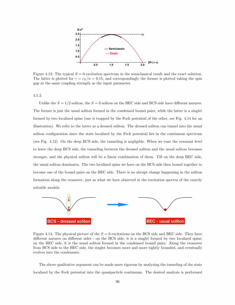
ϵF

--: Exact

—: Semiclassic

0.5 1.0 1.5 2.02P/(π n)

0.5

1.0

1.5

2.0

2.5

E/n2

Figure 4.13: The typical S = 0 excitation spectrum in the semiclassical result and the exact solution.The latter is plotted for γ = cF /n = 0.15, and correspondingly the former is plotted taking the spingap at the same coupling strength as the input parameter.

4.5.2.

Unlike the S = 1/2 soliton, the S = 0 soliton on the BEC side and BCS side have different natures.

The former is just the usual soliton formed in the condensed bound pairs, while the latter is a singlet

formed by two localized spins (one is trapped by the Fock potential of the other, see Fig. 4.14 for an

illustration). We refer to the latter as a dressed soliton. The dressed soliton can tunnel into the usual

soliton configuration since the state localized by the Fock potential lies in the continuous spectrum

(see Fig. 4.12). On the deep BCS side, the tunneling is negligible. When we tune the resonant level

to leave the deep BCS side, the tunneling between the dressed soliton and the usual soliton becomes

stronger, and the physical soliton will be a linear combination of them. Till on the deep BEC side,

the usual soliton dominates. The two localized spins we have on the BCS side then bound together to

become one of the bound pairs on the BEC side. There is no abrupt change happening in the soliton

formation along the crossover, just as what we have observed in the excitation spectra of the exactly

solvable models.

Figure 4.14: The physical picture of the S = 0 excitations on the BCS side and BEC side. They havedifferent natures on different sides - on the BCS side, it is a singlet formed by two localized spins;on the BEC side, it is the usual soliton formed in the condensed bound pairs. Along the crossoverfrom BCS side to the BEC side, the singlet becomes more and more tightly bounded, and eventuallyevolves into the condensate.

The above qualitative argument can be made more rigorous by analyzing the tunneling of the state

localized by the Fock potential into the quasiparticle continuum. The desired analysis is performed

96

for Eq. (4.81) in the regime where the chemical potential µ is the largest energy scale near the BCS

side, so the off-diagonal part can be treated perturbatively. We have both electron-like eigenstate |Ψe〉

and hole-like eigenstates∣∣Ψh

⟩at zeroth-order, and in each sector we will get a localized state

∣∣∣Ψe,h0

⟩.

Here we focus on the state∣∣Ψh

0

⟩with energy εh0 on the scale of µ, which will tunnel into the continuum

of the electron-like state |Ψek〉 as the off-diagonal perturbation sets in. The resonance width due to

this tunneling can be calculated using the Fermi golden rule:

Γ = 2πν↑,↓(2εF )|M|2 =1√2vF|M|2, (4.88)

where we have taken the density of states ν↑,↓(ε) = ν(ε)/2 for each spin to be the one at 2εF since

the localized level is close to the chemical potential µ, and M = 〈Ψek|

0 ∆

∆∗ 0

∣∣Ψh0

⟩is the matrix

element between the continuum and the localized state. It can be estimated by the Fourier component

∆(√

2kF ) of the soliton profile, normalized by the size of the soliton:

|M|2 =1

ls|∆(√

2kF )|2 =∆2

0lsπ2 sin2 θs

2

sinh2(lsπkF√

2

) . (4.89)

In the end we obtain the following result for the resonance width near the BCS side:

Γ =∆2

0lsπ2 sin2 θs

2√2vF sinh2

(lsπkF√

2

) . (4.90)

For the large chemical potential near the BCS side, the ratio between the resonance width Γ and

the energy εh0 is exponentially small and the localized state remains well-defined. This is equivalent

to the statement that the tunneling to the usual soliton is negligible. As we tune the system away

from the BCS side, up to the point where the chemical potential is comparable to the gap parameter

∆0, the velocity of the particle and the Fermi momentum are also tuned to be on the order of

magnitude comparable to ∆0. At that point, the resonance width Γ becomes comparable to the

energy εh0 . With further tuning toward the BEC side, we then encounter a large resonance width

Γ εh0 , and the localized state ceases to be well defined and merges into the quasiparticle continuum.

Correspondingly, we have the spin-singlet described on the BCS side develop into a normal bound

pair on the BEC side. As a result, we have a smooth crossover from the soliton of BCS type into the

one of BEC type.

97

4.6 Conclusion

In this chapter, we developed a semiclassical theory of moving solitons in one dimensional BCS-BEC

crossover, where on both the deep BCS and deep BEC side, our results grasp the essential features

of the exact solutions. Our theory also resolves the inconsistency between the semiclassical analysis

and the exact solutions in the attractive Yang-Gaudin model. In the meantime, we revealed the

mechanism of a striking phenomenon discussed in the previous chapter that the minimum energy of

the spin excitation is fixed at the Fermi momentum along the whole range of BCS-BEC crossover in

one dimension. Conventionally in higher dimensions, we would expect this momentum to be shifted

from kF on the BCS side to zero somewhere on the way to the BEC side, and it is believed that

this is the only sharp change that could happen in a BCS-BEC crossover [76]. We then show that

the counterintuitive fixing comes about as a special feature of the one dimensional systems, that

the conventional quasiparticle is not stable with respect to soliton formation. Our theory serves as

yet another example of the important role solitons can play in low dimensional physical systems, in

addition to those well established in one dimensional lattice models [97, 100] and charge density waves

[10, 11].

98

Bibliography

[1] S. K. Adhikari. Quantum scattering in two dimensions. American Journal of Physics, 54(4):362–

367, 1986. 6

[2] I. Affleck. On constrained instantons. Nuclear Physics B, 191(2):429 – 444, 1981. 82

[3] R. P. Anderson, C. Ticknor, A. I. Sidorov, and B. V. Hall. Spatially inhomogeneous phase

evolution of a two-component bose-einstein condensate. Phys. Rev. A, 80:023603, Aug 2009. 30

[4] N. Andrei and C. Destri. Solution of the multichannel kondo problem. Phys. Rev. Lett., 52:364–

367, Jan 1984. 41

[5] P. Bedaque, H.-W. Hammer, and U. van Kolck. The three-boson system with short-range

interactions. Nuclear Physics A, 646(4):444 – 466, 1999. 5

[6] F. F. Bellotti, T. Frederico, M. T. Yamashita, D. V. Fedorov, A. S. Jensen, and N. T. Zinner.

Scaling and universality in two dimensions: three-body bound states with short-ranged inter-

actions. Journal of Physics B: Atomic, Molecular and Optical Physics, 44(20):205302, 2011. 5,

23, 28

[7] F. F. Bellotti, T. Frederico, M. T. Yamashita, D. V. Fedorov, A. S. Jensen, and N. T. Zin-

ner. Supercircle description of universal three-body states in two dimensions. Phys. Rev. A,

85:025601, Feb 2012. 5, 23, 28

[8] F. F. Bellotti, T. Frederico, M. T. Yamashita, D. V. Fedorov, A. S. Jensen, and N. T. Zin-

ner. Mass-imbalanced three-body systems in two dimensions. Journal of Physics B: Atomic,

Molecular and Optical Physics, 46(5):055301, 2013. 5, 23, 28

[9] E. Braaten and H.-W. Hammer. Universality in few-body systems with large scattering length.

Physics Reports, 428(56):259 – 390, 2006. 5

99

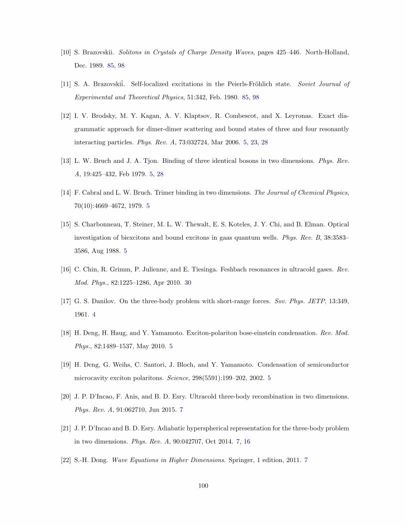
[10] S. Brazovskii. Solitons in Crystals of Charge Density Waves, pages 425–446. North-Holland,

Dec. 1989. 85, 98

[11] S. A. Brazovskii. Self-localized excitations in the Peierls-Frohlich state. Soviet Journal of

Experimental and Theoretical Physics, 51:342, Feb. 1980. 85, 98

[12] I. V. Brodsky, M. Y. Kagan, A. V. Klaptsov, R. Combescot, and X. Leyronas. Exact dia-

grammatic approach for dimer-dimer scattering and bound states of three and four resonantly

interacting particles. Phys. Rev. A, 73:032724, Mar 2006. 5, 23, 28

[13] L. W. Bruch and J. A. Tjon. Binding of three identical bosons in two dimensions. Phys. Rev.

A, 19:425–432, Feb 1979. 5, 28

[14] F. Cabral and L. W. Bruch. Trimer binding in two dimensions. The Journal of Chemical Physics,

70(10):4669–4672, 1979. 5

[15] S. Charbonneau, T. Steiner, M. L. W. Thewalt, E. S. Koteles, J. Y. Chi, and B. Elman. Optical

investigation of biexcitons and bound excitons in gaas quantum wells. Phys. Rev. B, 38:3583–

3586, Aug 1988. 5

[16] C. Chin, R. Grimm, P. Julienne, and E. Tiesinga. Feshbach resonances in ultracold gases. Rev.

Mod. Phys., 82:1225–1286, Apr 2010. 30

[17] G. S. Danilov. On the three-body problem with short-range forces. Sov. Phys. JETP, 13:349,

1961. 4

[18] H. Deng, H. Haug, and Y. Yamamoto. Exciton-polariton bose-einstein condensation. Rev. Mod.

Phys., 82:1489–1537, May 2010. 5

[19] H. Deng, G. Weihs, C. Santori, J. Bloch, and Y. Yamamoto. Condensation of semiconductor

microcavity exciton polaritons. Science, 298(5591):199–202, 2002. 5

[20] J. P. D’Incao, F. Anis, and B. D. Esry. Ultracold three-body recombination in two dimensions.

Phys. Rev. A, 91:062710, Jun 2015. 7

[21] J. P. D’Incao and B. D. Esry. Adiabatic hyperspherical representation for the three-body problem

in two dimensions. Phys. Rev. A, 90:042707, Oct 2014. 7, 16

[22] S.-H. Dong. Wave Equations in Higher Dimensions. Springer, 1 edition, 2011. 7

100

[23] L.-M. Duan, E. Demler, and M. D. Lukin. Controlling spin exchange interactions of ultracold

atoms in optical lattices. Phys. Rev. Lett., 91:090402, Aug 2003. 30

[24] A. R. Edmonds. Angular Momentum in Quantum Mechanics. Princeton University Press, 1996.

7

[25] D. K. Efimkin and V. Galitski. Moving solitons in a one-dimensional fermionic superfluid. Phys.

Rev. A, 91:023616, Feb 2015. 69, 70, 72, 87, 93

[26] V. Efimov. Energy levels arising from resonant two-body forces in a three-body system. Physics

Letters B, 33(8):563 – 564, 1970. 1, 4

[27] V. Efimov. Weakly-bound states of three resonantly interacting particles. Sov.J.Nucl.Phys., 12,

May 1971. 1, 4

[28] M. Erhard, H. Schmaljohann, J. Kronjager, K. Bongs, and K. Sengstock. Measurement of a

mixed-spin-channel feshbach resonance in 87Rb. Phys. Rev. A, 69:032705, Mar 2004. 30

[29] L. D. Faddeev. Mathematical Aspects of the Three-Body Problem in the Quantum Scattering

Theory. Israel Program for Scientific Translations, 1965. 7

[30] L. D. Faddeev and L. Takhtajan. Hamiltonian Methods in the Theory of Solitons. Springer-

Verlag, Berlin, 1987. 85

[31] H. S. Friedrich. Theoretical Atomic Physics. Springer Science and Business Media, 3 edition,

2005. 14, 22

[32] J. N. Fuchs, A. Recati, and W. Zwerger. Exactly solvable model of the bcs-bec crossover. Phys.

Rev. Lett., 93:090408, Aug 2004. 32, 52, 55

[33] P. Fulde and R. A. Ferrell. Superconductivity in a strong spin-exchange field. Phys. Rev.,

135:A550–A563, Aug 1964. 31

[34] B. Ganchev, N. Drummond, I. Aleiner, and V. Fal’ko. Three-particle complexes in two-

dimensional semiconductors. Phys. Rev. Lett., 114:107401, Mar 2015. 5, 11

[35] M. Gaudin. Un systeme a une dimension de fermions en interaction. Physics Letters A, 24(1):55

– 56, 1967. 31, 32, 66

[36] M. Gaudin. The Bethe Wavefunction. Cambridge University Press, 2014. 49

101

[37] L. S. Gradstein and I. M. Ryzhik. Tables of Integrals, Series and Products. Academic Press, 6

edition, 2000. 17, 24, 26, 27

[38] S.-J. Gu, Y.-Q. Li, Z.-J. Ying, and X.-A. Zhao. Thermodynamics of two component bosons in

one dimension. International Journal of Modern Physics B, 16(14n15):2137–2143, 2002. 31

[39] X. W. Guan, M. T. Batchelor, and C. Lee. Fermi gases in one dimension: From bethe ansatz

to experiments. Rev. Mod. Phys., 85:1633–1691, Nov 2013. 32, 69, 72

[40] X. W. Guan, M. T. Batchelor, C. Lee, and M. Bortz. Phase transitions and pairing signature

in strongly attractive fermi atomic gases. Phys. Rev. B, 76:085120, Aug 2007. 60, 62

[41] X. W. Guan and T. L. Ho. Quantum criticality of a one-dimensional attractive fermi gas. Phys.

Rev. A, 84:023616, Aug 2011. 60

[42] V. Gurarie. One-dimensional gas of bosons with feshbach-resonant interactions. Phys. Rev. A,

73:033612, Mar 2006. 31, 33, 41

[43] F. D. M. Haldane. Luttinger liquid theory of one-dimensional quantum fluids. i. properties of

the luttinger model and their extension to the general 1d interacting spinless fermi gas. Journal

of Physics C: Solid State Physics, 14(19):2585–2609, Jul 1981. 1

[44] E. Haller, M. Gustavsson, M. J. Mark, J. G. Danzl, R. Hart, G. Pupillo, and H.-C. Nagerl.

Realization of an excited, strongly correlated quantum gas phase. Science, 325(5945):1224–

1227, 2009. 30

[45] H.-W. Hammer and L. Platter. Efimov physics from a renormalization group perspective. Phil.

Trans. Roy. Soc. Lond., A369:2679, 2011. 5

[46] P. C. Hohenberg. Existence of long-range order in one and two dimensions. Phys. Rev., 158:383–

386, Jun 1967. 1

[47] H. Hu, X.-J. Liu, and P. D. Drummond. Phase diagram of a strongly interacting polarized fermi

gas in one dimension. Phys. Rev. Lett., 98:070403, Feb 2007. 60

[48] L. Hulten. Ark. Mat. Astron. Fys. B., 26A:1, 1938. 38

[49] V. Hutson. The circular plate condenser at small separations. Mathematical Proceedings of the

Cambridge Philosophical Society, 59(1):211–224, 1963. 49

102

[50] T. Iida and M. Wadati. Exact analysis of δ-function attractive fermions and repulsive bosons

in one-dimension. Journal of the Physical Society of Japan, 74(6):1724–1736, 2005. 49

[51] A. Imambekov, A. A. Lukyanov, L. I. Glazman, and V. Gritsev. Exact solution for 1d spin-

polarized fermions with resonant interactions. Phys. Rev. Lett., 104:040402, Jan 2010. 33,

41

[52] M. Iskin. Dimer-atom scattering between two identical fermions and a third particle. Phys. Rev.

A, 81:043634, Apr 2010. 28

[53] O. I. Kartavtsev and A. V. Malykh. Universal low-energy properties of three two-dimensional

bosons. Phys. Rev. A, 74:042506, Oct 2006. 7

[54] J. Kasprzak et al. Nature, 443:409–414, Sep 2006. 5

[55] M. Khodas, A. Kamenev, and L. I. Glazman. Photosolitonic effect. Phys. Rev. A, 78:053630,

Nov 2008. 71, 89, 92

[56] T. Kinoshita, T. Wenger, and D. S. Weiss. Observation of a one-dimensional tonks-girardeau

gas. Science, 305(5687):1125–1128, 2004. 30

[57] A. Klauser and J.-S. Caux. Equilibrium thermodynamic properties of interacting two-component

bosons in one dimension. Phys. Rev. A, 84:033604, Sep 2011. 31

[58] V. E. Korepin, N. M. Bogoliubov, and A. G. Izergin. Quantum Inverse Scattering Method and

Correlation Functions. Cambridge University Press, UK, 1993. 31, 35, 36, 37, 39, 46, 53

[59] V. Y. Krivnov and A. A. Ovchinnikov. One-dimensional Fermi gas with attraction between the

electrons. Soviet Journal of Experimental and Theoretical Physics, 40:781, Oct. 1975. 52, 55, 59

[60] P. P. Kulish, S. V. Manakov, and L. D. Faddeev. Comparison of the Exact Quantum and

Quasiclassical Results for the Nonlinear Schrodinger Equation. Theor. Math. Phys., 28:615–

620, 1976. [Teor. Mat. Fiz.28,38(1976)]. 69, 71, 89, 92

[61] L. D. Landau and L. M. Lifshitz. Quantum Mechanics: Non-Relativistic Theory, volume 3.

Butterworth-Heinemann, 3 edition, 1981. 6

[62] A. I. Larkin and Y. N. Ovchinnikov. Nonuniform state of superconductors. Zh. Eksp. Teor.

Fiz., 47:1136–1146, Sep 1964. 31

103

[63] J. Levinsen and V. Gurarie. Properties of strongly paired fermionic condensates. Phys. Rev. A,

73:053607, May 2006. 28

[64] J. Levinsen, P. Massignan, and M. M. Parish. Efimov trimers under strong confinement. Phys.

Rev. X, 4:031020, Jul 2014. 28

[65] Y.-A. Liao, A. S. C. Rittner, T. Paprotta, W. Li, G. B. Partridge, R. G. Hulet, S. K. Baur, and

E. J. Mueller. Spin-imbalance in a one-dimensional fermi gas. Nature, 467(7315):567–569, 09

2010. 30

[66] E. H. Lieb. Exact analysis of an interacting bose gas. ii. the excitation spectrum. Phys. Rev.,

130:1616–1624, May 1963. 30, 32, 53, 55, 69

[67] E. H. Lieb and W. Liniger. Exact analysis of an interacting bose gas. i. the general solution and

the ground state. Phys. Rev., 130:1605–1616, May 1963. 30, 32, 49, 52, 65, 69

[68] Q.-G. Lin. Levinson theorem in two-dimensions. Phys. Rev., A56:1938–1944, 1997. 14, 22

[69] MATLAB. version 9.0.0 (R2016a). The MathWorks Inc., Natick, Massachusetts, 2016. 22

[70] N. D. Mermin and H. Wagner. Absence of ferromagnetism or antiferromagnetism in one- or

two-dimensional isotropic heisenberg models. Phys. Rev. Lett., 17:1133–1136, Nov 1966. 1

[71] K. M. Mertes, J. W. Merrill, R. Carretero-Gonzalez, D. J. Frantzeskakis, P. G. Kevrekidis, and

D. S. Hall. Nonequilibrium dynamics and superfluid ring excitations in binary bose-einstein

condensates. Phys. Rev. Lett., 99:190402, Nov 2007. 30

[72] R. Miller and D. Kleinman. Excitons in gaas quantum wells. Journal of Luminescence, 30(1):520

– 540, 1985. 5

[73] R. C. Miller, D. A. Kleinman, A. C. Gossard, and O. Munteanu. Biexcitons in gaas quantum

wells. Phys. Rev. B, 25:6545–6547, May 1982. 5

[74] H. Moritz, T. Stoferle, M. Kohl, and T. Esslinger. Exciting collective oscillations in a trapped

1d gas. Phys. Rev. Lett., 91:250402, Dec 2003. 30

[75] G. Orso. Attractive fermi gases with unequal spin populations in highly elongated traps. Phys.

Rev. Lett., 98:070402, Feb 2007. 60

[76] M. M. Parish. The BCS-BEC Crossover, pages 179–197. World Scientific Publishing Co, Sept.

2015. 53, 70, 72, 74, 98

104

[77] F. M. Pen’kov and W. Sandhas. Differential form of the skornyakov ter-martirosyan equations.

Phys. Rev. A, 72:060702, Dec 2005. 29

[78] D. S. Petrov. Three-body problem in fermi gases with short-range interparticle interaction.

Phys. Rev. A, 67:010703, Jan 2003. 28

[79] D. S. Petrov. Quantum mechanical stabilization of a collapsing bose-bose mixture. Phys. Rev.

Lett., 115:155302, Oct 2015. 6

[80] D. S. Petrov and G. E. Astrakharchik. Ultradilute low-dimensional liquids. Phys. Rev. Lett.,

117:100401, Sep 2016. 6

[81] D. S. Petrov, C. Salomon, and G. V. Shlyapnikov. Weakly bound dimers of fermionic atoms.

Phys. Rev. Lett., 93:090404, Aug 2004. 28

[82] D. S. Petrov and G. V. Shlyapnikov. Interatomic collisions in a tightly confined bose gas. Phys.

Rev. A, 64:012706, Jun 2001. 6

[83] L. Pollet, S. M. A. Rombouts, and P. J. H. Denteneer. Ultracold atoms in one-dimensional

optical lattices approaching the tonks-girardeau regime. Phys. Rev. Lett., 93:210401, Nov 2004.

30

[84] G. Poschl and E. Teller. Bemerkungen zur quantenmechanik des anharmonischen oszillators.

Zeitschrift fur Physik, 83(3):143–151, Mar 1933. 90

[85] A. Prem and V. Gurarie. One-dimensional model of chiral fermions with feshbach resonant

interactions. Journal of Statistical Mechanics: Theory and Experiment, 2018(2):023111, 2018.

33

[86] S. Rahbar and E. Hashemizadeh. A computational approach to the fredholm integral equation

of the second kind. Proceedings of the World Congress on Engineering, 2, 2008. 46

[87] T. Ren and I. Aleiner. Three-boson bound states in two dimensions. Phys. Rev. B, 95:045401,

Jan 2017. 6

[88] T. Ren and I. Aleiner. Bethe-ansatz analysis of near-resonant two-component systems in one

dimension. Phys. Rev. A, 99:023611, Feb 2019. 30, 71

[89] T. Ren and I. Aleiner. Solitons in one-dimensional systems at the bcs-bec crossover. Phys. Rev.

A, 99:013626, Jan 2019. 59

105

[90] S. T. Rittenhouse, N. P. Mehta, and C. H. Greene. Green’s functions and the adiabatic hyper-

spherical method. Phys. Rev. A, 82:022706, Aug 2010. 7, 16

[91] S. Rudin. One-dimensional backward-scattering fermion model with built-in cutoff. Phys. Rev.

B, 28:4825–4828, Oct 1983. 41

[92] P. Schlottmann. Thermodynamics of the one-dimensional multicomponent fermi gas with a

delta -function interaction. Journal of Physics: Condensed Matter, 5(32):5869, 1993. 31

[93] P. Schlottmann. Ground-state and elemental excitations of the one-dimensional multicomponent

fermi gas with delta -function interaction. Journal of Physics: Condensed Matter, 6(7):1359,

1994. 31

[94] J. R. Schrieffer. Theory of Superconductivity, Section 2.5. Westview Press, 1983. 75

[95] S. S. Shamailov and J. Brand. Dark-soliton-like excitations in the yang-gaudin gas of attractively

interacting fermions. New Journal of Physics, 18(7):075004, 2016. 69, 70, 72, 93

[96] G. V. Skorniakov and K. A. Ter-Martirosian. Sov. Phys. JETP, 4:648, 1957. 4

[97] W. P. Su, J. R. Schrieffer, and A. J. Heeger. Soliton excitations in polyacetylene. Phys. Rev. B,

22:2099–2111, Aug 1980. 85, 98

[98] B. Sutherland. Beautiful Models: 70 Years of Exactly Solved Quantum Many-Body Problems.

World Scientific, June 2004. 31, 41

[99] M. Takahashi. Thermodynamics of One-Dimensional Solvable Models. Cambridge University

Press, UK, 1999. 62

[100] H. Takayama, Y. R. Lin-Liu, and K. Maki. Continuum model for solitons in polyacetylene.

Phys. Rev. B, 21:2388–2393, Mar 1980. 85, 87, 98

[101] F. Tassone and Y. Yamamoto. Exciton-exciton scattering dynamics in a semiconductor mi-

crocavity and stimulated scattering into polaritons. Phys. Rev. B, 59:10830–10842, Apr 1999.

6

[102] N. Y. K. Tim Byrnes and Y. Yamamoto. Exciton-polariton condensates. Nat. Phys., 10, Nov

2014. 5

[103] I. V. Tokatly. Dilute fermi gas in quasi-one-dimensional traps: From weakly interacting fermions

via hard core bosons to a weakly interacting bose gas. Phys. Rev. Lett., 93:090405, Aug 2004.

32

106

[104] T. Tsuzuki. Nonlinear waves in the pitaevskii-gross equation. Journal of Low Temperature

Physics, 4(4):441–457, Apr 1971. 89

[105] L. A. Samaj and Z. Bajnok. Introduction to the Statistical Physics of Integrable Many-body

Systems. Cambridge University Press, UK, May 2013. 31, 35, 36, 37, 53, 65, 114

[106] A. H. van Amerongen, J. J. P. van Es, P. Wicke, K. V. Kheruntsyan, and N. J. van Druten.

Yang-yang thermodynamics on an atom chip. Phys. Rev. Lett., 100:090402, Mar 2008. 30

[107] M. Wadati and K. Ohkuma. Bethe states for the quantum three wave interaction equation.

Journal of the Physical Society of Japan, 53(4):1229–1237, 1984. 33

[108] A. Widera, S. Trotzky, P. Cheinet, S. Folling, F. Gerbier, I. Bloch, V. Gritsev, M. D. Lukin,

and E. Demler. Quantum spin dynamics of mode-squeezed luttinger liquids in two-component

atomic gases. Phys. Rev. Lett., 100:140401, Apr 2008. 30

[109] C. N. Yang. Some exact results for the many-body problem in one dimension with repulsive

delta-function interaction. Phys. Rev. Lett., 19:1312–1315, Dec 1967. 31, 32, 66

[110] C. N. Yang. s matrix for the one-dimensional n-body problem with repulsive or attractive

δ-function interaction. Phys. Rev., 168:1920–1923, Apr 1968. 31, 32

[111] V. E. Zakharov and A. B. Shabat. Exact Theory of Two-dimensional Self-focusing and One-

dimensional Self-modulation of Waves in Nonlinear Media. Soviet Journal of Experimental and

Theoretical Physics, 34:62, 1972. 89

[112] V. E. Zakharov and A. B. Shabat. Interaction between solitons in a stable medium. Soviet

Journal of Experimental and Theoretical Physics, 37:823, Nov. 1973. 89

107

Appendix A

Calculation of the Matrix Elements

of the Berry Connection

Here we calculate the matrix elements of the Berry connection for the case with zero angular momen-

tum m = 0. Firstly we verify the orthogonality of the eigenstates χi(n) in Eq. (2.50) and calculate

the normalization factor Ni in Eq. (2.62) via the overlap integral:

〈χi| χj〉 =1

8π2

∫ 1

−1

dx

∫ 2π

0

dφ1dφ2 χi(n)χj(n). (A.1)

Substituting the expression in Eq. (2.50) into the above integral, we will get

〈χi| χj〉 = (αiαj + 2βiβj)I1 + 2(αiβj + αjβi + βiβj)I2, (A.2)

where the two integral I1,2 are

I1 ≡1

8π2

∫ 1

−1

dx

∫ 2π

0

dφ1dφ2 Gνi(n · n1)Gνj (n · n1),

I2 ≡1

8π2

∫ 1

−1

dx

∫ 2π

0

dφ1φ2 Gνi(n · n1)Gνj (n · n2).

(A.3)

Substituting Eq. (2.48) into Eq. (A.3) and performing the integration, we will get

I1 =1

4π

1

(νi − νj)(νi + νj + 1)

[Gνi(x)−Gνj (x)

]x→1

,

I2 =1

4π

1

(νi − νj)(νi + νj + 1)

[Gνi(x)−Gνj (x)

]x=− 1

2

.

(A.4)

108

Substitute these back into the overlap integral in Eq. (A.1), and apply the constraint on coefficients

(αi, βi) in Eq. (2.51), we finally arrived at

〈χi| χj〉 =

0 (i 6= j)[

(α2i+2β2

i )∂νiGνi (1)+[2β2i+4αiβi]∂νiGνi(− 1

2 )]

(4π)(2νi+1) (i = j)

. (A.5)

Secondly we try to calculate the matrix element of the Berry connection in Eq. (2.37). The scale

dependence only appears in the regularized Green’s function Gνi(1), thus the relevant quantity that

contributes to the derivative with respect to ln r is inside integral I1:

I1 =1

4π

1

(νi − νj)((νi + νj + 1)

1

2πlnrirj

+ (· · · ), (A.6)

where we have used the expression for Gνi(1) in Eq. (2.49), and the scale r is equipped with subscript

to differentiate between |χi〉 and |χj〉. The derivative involved in Eq. (2.37) is then performed with

respect to ri and we finally get the expression for the matrix element Dij as

Dij =(αiαj + 2βiβj)

8π2√NiNj(νi − νj)(νi + νj + 1)

, (A.7)

with the normalization factor Ni given by 〈χi| χi〉.

109

Appendix B

First Order Correction to

Adiabatics

In this section we present the detail of calculation of the first order correction to the effective potential

u0 in Eq. (2.63) and obtain the result in Eq. (2.69). Using the matrix Hamiltonian H(ν) in Eq. (2.65)

and normalization condition in Eq. (2.68), together with the expression for the first order correction

in Eq. (2.61), we arrive at the following expression:

|D0j |2 =(2ν0 + 1)(2νj + 1)

[ν0(ν0 + 1)− νj(νj + 1)]2Tr[~α0 · ~αT0 · ~αj · ~αTj ]

∂ν0det H ∂νj det H

=(2ν0 + 1)(2νj + 1)

[ν0(ν0 + 1)− νj(νj + 1)]2Tr[det H0 · H−1

0 det Hj · H−1j ]

∂ν0 det H ∂νj det H.

(B.1)

The last line can be further simplified to the following form using the residuals of K = H−1:

|D0j |2 =(2ν0 + 1)(2νj + 1)

[ν0(ν0 + 1)− νj(νj + 1)]2Tr[Res K(ν0) · Res K(νj)]. (B.2)

The total correction ∆u0 in Eq. (2.63) can then be converted into a contour integration on the complex

plane of variable ν, where the integration contour is along the real axis. On that complex plane, each

νj is a first-order pole along the positive real axis, and each have its counterpart on the negative real

axis. There are four extra poles off real axis, corresponding to true bound state (ν0) and spurious

110

bound state (νs) respectively (see Fig. 2.7). Finally the expression for ∆u0 are as follows:

∑j 6=0

|D0j |2 =∑j 6=0

(2ν0 + 1)(2νj + 1)

[ν0(ν0 + 1)− νj(νj + 1)]2Tr[Res K(ν0) · Res K(νj)]

=∑j 6=0

∂

∂ν0

[− 1

ν0 − νj+

1

ν0 + νj + 1

]Tr[Res K(ν0) · Res K(νj)]

=1

2

1

2πi

∮Cdν

Tr[Res K(ν0) · K(ν)]

(ν0 − ν)2− 1

2πi

∮Cdν

Tr[Res K(ν0) · K(ν)]

(ν0 + ν + 1)2

=1

2

1

2πi

∮Cdν

Tr[Res K(ν0) · K(ν)]

(ν0 − ν)2+

1

2πi

∮Cdν

Tr[Res K(ν∗0 ) · K(ν)]

(ν∗0 − ν)2

,

(B.3)

where we have used the fact that Res K(ν0) = −Res K(ν∗0 ) and the factor 1/2 appears because we

are only summing over positive real poles. This is nothing but Eq. (2.69) in the main text.

To evaluate the resulting contour integrals in Eq. (2.69), we only care about the behavior of the

integrand around the poles far off the real axis. The large ν behavior is

H(ν)∣∣∣|ν|1

=

A(ν) 0

0 B(ν)

, K(ν) = (ν) =

1A(ν) 0

0 1B(ν)

,

A(ν) = lnr

α<− 1

2[ψ(−ν) + ψ(ν + 1)], B(ν) = ln

r

α>− 1

2[ψ(−ν) + ψ(ν + 1)].

(B.4)

The poles off the real axis are given by zeros of the diagonal functions A(ν) and B(ν). Near the poles,

taking ν0 as an example, we have A(ν0) 6= 0 and

B(ν) = B′(ν − ν0) +1

2B′′(ν − ν0)2 +

1

6B′′′(ν − ν0)3 + · · · ,

1

B(ν)=

1

B′(ν − ν0)− 1

2

B′′

B′2−[ B′′′

6B′2− B′′2

4B′3

](ν − ν0) + · · · ,

(B.5)

where the coefficients B′, B′′, B′′′ are

B′ =2i

(|u0| − 1)1/2, B′′ = − 4

|u0| − 1, B′′′ = − 16i

(|u0| − 1)3/2. (B.6)

The the residual and the regular part of K(ν) near ν = ν0 is

Res K(ν0) =

0 0

0 1B′

, Kreg,ν0(ν) =

1A(ν) 0

0 − 12B′′

B′2 −[B′′′

6B′2 − B′′2

4B′3

](ν − ν0) + · · ·

. (B.7)

111

Substituting the above expression into the contour integral in Eq. (2.69), we obtain

1

2πi

∮C

dνTr[Res K(ν0) · K(ν)]

(ν0 − ν)2+

1

2πi

∮C

dνTr[Res K(ν∗0 ) · K(ν)]

(ν∗0 − ν)2

=− ∂

∂νTr[Res K(ν0) · Kreg,ν0(ν)]

∣∣∣ν=ν0

− Tr[Res K(ν0) · Res K(ν∗0 )]

(ν0 − ν∗0 )2

− Tr[Res K(ν∗0 ) · Res K(ν0)]

(ν∗0 − ν0)2− ∂

∂νTr[Res K(ν∗0 ) · Kreg,ν∗0 (ν)]

∣∣∣ν=ν∗0

,

(B.8)

where the contribution from the unphysical poles ν = νs, ν∗s is zero because they reside at different

corner along the diagonal, which makes the trace of the matrix product zero. Finally, the first order

correction to the adiabatic approximation is evaluated to be

∑j

|D0j |2 =

[B′′′

6B′3− B′′2

4B′4+

1

B′2(ν0 − ν∗0 )2

]=

1

3, (B.9)

which combined with Eq. (2.59) gives us the marginal result γ = 1.

Similarly we can calculate the same first order correction to adiabatics for the case of non-zero

angular momentum m. By direct calculation similar to the case of zero angular momentum we obtain

the following result for the Berry connection Dij :

Dij =1

8π2√NiNj

∫ 1

−1

dx

∫ 2π

0

dφ1dφ2dχ

(m)i (n)

d ln rχ

(m)j (n)

=1

8π2√NiNj

(αiαj + 2βiβj)1

2m1

(νi − νj)(νi + νj +m+ 1),

(B.10)

where the normalization factor Ni of the angular eigenfunctions is calculated to be

Ni =

[(α2i + 2β2

i )∂νiG(m)νi (1) + [2(−)mβ2

i + 4αiβi]∂νiG(m)νi (− 1

2 )]

2m(4π)(2νi +m+ 1), (B.11)

and the single-argument Green’s function is defined as

G(m)ν (x) =

(1 + x

2

)m/2f(ν,m)R(m)

ν

(1 + x

2

), (B.12)

where the functions f(ν,m) and R(m)ν (x) are defined in Eq. (2.82) and Eq. (2.72). For the correction

to the effective potential of the lowest level, we still have

∆u(m)0 (r →∞) =

∑j 6=0

|D0j |2. (B.13)

112

This can be calculated exactly the same way as the case m = 0. The only change is the expression

for the matrix Hamiltonian H(ν):

H(ν) = 2π

1λ1

+G(m)ν (1);

√2G

(m)ν

(− 1

2

)√

2G(m)ν

(− 1

2

); G

(m)ν (1) + (−)mG

(m)ν

(− 1

2

)− 1

λ2

. (B.14)

The rest of the calculation is essentially the same as the case m = 0, and the contour integration trick

eventually gives us the following result:

∆u(m)0 (r →∞) = 1/3,

u(m)0 (r →∞) = −r2ε

(2)b + (m2 − 1) +O(r−2).

(B.15)

This shows that the marginal value γ = 1 is only realized when m = 0; for non-zero angular momen-

tum, no bound state is guaranteed for the system.

113

Appendix C

Algebraic Bethe Ansatz for

Two-Component Systems

This appendix closely follows the derivation presented in [105]. For a time inversion and space inversion

invariant and species-conserving model in free space, the two-body S-matrix in pseudospin subspace

↑, ↓ assumes the general form in Eq. (3.11), which is repeated here:

S(k) =

a(k) 0 0 0

0 b(k) c(k) 0

0 c(k) b(k) 0

0 0 0 a(k)

, (C.1)

where the relative momentum k = k2 − k1 is the difference in momentum between the two scattering

particles. The wave functions of the eigenstates then assumes the general form of the nested coordinate

Bethe ansatz in Eq. (3.123), which is also repeated here:

ΨX(σ1, x1; · · · ;σN , xN ) =∑P∈SN

[X,P ] exp

i N∑j=1

kPjxXj

,

[X,P ] = sgn(X)sgn(P )AσX1σX2···σXN (kP1

, kP2, · · · , kPN ),

(C.2)

where X denotes the ordering sector with xX1< xX2

< · · · < xXN and P denotes the permutation

among the wave numbers. The sign function equals 1 for even permutations and −1 for odd permu-

tations. We impose the periodic boundary condition for the wave functions, so the wave functions are

114

invariant under the following shift of coordinates:

xX1 = xX1 + L, xX2 = xX2 , . . . , xXN = xXN . (C.3)

This shift brings the ordering sector X : xX1< xX2

< · · · < xXN to X : xX2< xX3

< · · · < xXN <

XX1, and the invariance of the wave functions is equivalent to the relation

AσX2···σXN σX1

(kP2 , · · · , kPN , kP1) = (∓1)N−1 exp (−ikP1L)AσX1···σXN (kP1 , · · · , kPN ) , (C.4)

where the upper minus sign is for bosons, and the lower plus sign is for fermions. The A-coefficients

can be related to each other via the two-body S-matrix:

A···σjσi··· (· · · , kv, ku, · · · ) =∑σ′iσ′j

Sσiσjσ′iσ′j

(ku, kv)A···σ′iσ′j ··· (· · · , ku, kv, · · · ) . (C.5)

Using Eq. (C.5), we can transform the condition in Eq. (C.4) into an eigenvalue problem:

TjA = (∓1)N−1 exp (−ikjL)A, (C.6)

where the transfer matrix Tj is defined as

Tj = T (k = kj ; k1, · · · , kN ) ,

T (k; k1, · · · , kN )σ1···σNσ′1···σ′N =

∑γ1,...,γN

SσNγ1

σ′Nγ2(k − kN )S

σN−1γ2

σ′N−1γ3(k − kN−1) · · ·Sσ2γN−1

σ′2γN(k − k2)Sσ1γN

σ′1γ1(k − k1) .

(C.7)

The transfer matrix T (k; k1, · · · , kN ) is usually referred to as the inhomogeneous transfer matrix, and

it can be obtained as the trace of the monodromy matrix T in the auxiliary ξ-space:

T (k; k1, · · · , kN ) = Trξ Tξ (k; k1, · · · , kN ) , (C.8)

where the monodromy matrix T is the product of Lax matrices Lξn:

Tξ (k; k1, · · · , kN ) = LξN (k − kN )Lξ(N−1) (k − kN−1) · · ·Lξ1 (k − k1) ,

Lξn(k)γξσ1...σNγ′ξσ′1...σ

′N

= Sγξσnγ′ξσ′n

(k)δσ1σ′1· · · δσn−1σ′n−1

δσn+1σ′n+1· · · δσNσ′N .

(C.9)

115

Using the above definitions, we can express the monodromy matrix in the auxiliary ξ-space:

T (k; k1, · · · , kN ) =

A (k; k1, · · · , kN ) B (k; k1, · · · , kN )

C (k; k1, · · · , kN ) D (k; k1, . . . , kN )

. (C.10)

The matrices A,B,C and D fulfills the following commutation relations as a result of the Yang-Baxter

equation:

[A(k), A(k′)] = [B(k), B(k′)] = [C(k), C(k′)] = [D(k), D(k′)] = 0,

A(k)B(k′) =a(k′ − k)

b(k′ − k)B(k′)A(k)− c(k′ − k)

b(k′ − k)B(k)A(k′),

D(k)B(k′) =a(k − k′)b(k − k′)B(k′)D(k)− c(k − k′)

b(k − k′)B(k)D(k′),

(C.11)

where a, b and c are the matrix elements of the two-body S-matrix. The inhomogeneous transfer

matrix can be expressed as the trace of T in the auxiliary ξ-space:

T (k; k1, · · · , kN ) = A (k; k1, · · · , kN ) +D (k; k1, · · · , kN ) . (C.12)

Next, we want to diagonalize the inhomogeneous matrix T . We first construct a generating vector of

the 2N -dimensional Hilbert space as the tensor product of spin-up vectors on the chain of N sites:

Ω = e+︸︷︷︸1

⊗ e+︸︷︷︸2

⊗ · · · ⊗ e+︸︷︷︸N−1

⊗ e+︸︷︷︸N

, e+ =

1

0

. (C.13)

The actions of the matrix elements of the monodromy matrix on this generating vector give us the

following results:

AΩ =

N∏n=1

a (λ− λn) Ω, CΩ = 0, DΩ =

N∏n=1

b (λ− λn) Ω. (C.14)

The eigenvectors of the inhomogeneous transfer matrix with M spins down are assumed to be in the

following form:

ψ (k1, · · · , kN ; Λ1, · · · ,ΛM ) =

M∏α=1

B (Λα; k1, · · · , kN ) Ω, (C.15)

where the parameters Λ1, · · · ,ΛM are yet to be determined. Using the commutation relations in

Eq. (C.11) and the results in Eq. (C.14), we can obtain the conditions for the ansatz in Eq. (C.15) to

116

be eigenvectors of the inhomogeneous transfer matrix T = A+D:

N∏n=1

a(Λα − kn)

b(Λα − kn)=

M∏β=1β 6=α

a(Λα − Λβ)b(Λβ − Λα)

a(Λβ − Λα)b(Λα − Λβ), α = 1, 2 · · · ,M. (C.16)

In the meantime, the periodic boundary conditions as specified in Eq. (C.6) take the following form:

(∓)N−1 exp(−ikjL) =

N∏n=1

a(kj − kn)

M∏α=1

a(Λα − kj)b(Λα − kj)

, j = 1, 2, · · · , N. (C.17)

The M + N coupled equations in Eq. (C.16) and Eq. (C.17) are those specified in Eq. (3.15) of the

main text, which are referred to as the Bethe ansatz equations.

117