Faculty of Electrical Engineering Department of Electrical Engineering Supervisor: Dr. Benny Lövström Blekinge Institute of Technology SE-371 79 Karlskrona Sweden

Contrast Enhancement of Colour Images using Transform Based Gamma Correction

and Histogram Equalization

Pruthvi Venkatesh Gatti Krishna Teja Velugubantla

ii

This thesis is submitted to the Faculty of Engineering at Blekinge Institute of Technology in partial fulfillment of the requirements for the degree of Master of Science in Electrical Engineering. The thesis is equivalent to 20 weeks of full time studies.

Contact Information: Author(s): Pruthvi Venkatesh Gatti E-mail: prga15@student.bth.se Krishna Teja Velugubantla E-mail: krve15@student.bth.se

University advisor: Assoc. Prof. Benny Lövström Department of Applied Signal Processing

Faculty of Engineering Blekinge Institute of Technology SE-371 79 Karlskrona, Sweden

Internet : www.bth.se Phone : +46 455 38 50 00 Fax : +46 455 38 50 57

i

ABSTRACT Contrast is an important factor in any subjective evaluation of image quality. It is the difference in visual properties that makes an object distinguishable from other objects and background. Contrast Enhancement method is mainly used to enhance the contrast in the image by using its Histogram. Histogram is a distribution of numerical data in an image using graphical representation. Histogram Equalization is widely used in image processing to adjust the contrast in the image using histograms. Whereas Gamma Correction is often used to adjust luminance in an image. By combining Histogram Equalization and Gamma Correction we proposed a hybrid method, that is used to modify the histograms and enhance contrast of an image in a digital method. Our proposed method deals with the variants of histogram equalization and transformed based gamma correction. Our method is an automatically transformation technique that improves the contrast of dimmed images via the gamma correction and probability distribution of luminance pixels. The proposed method is converted into an android application. We succeeded in enhancing the contrast of an image by using our method and we have tested for different alpha values. Graphs of the gamma for different alpha values are plotted.

Keywords: Contrast Enhancement, Image Processing, Traditional Histogram Equalization, Transformed Based Gamma Correction.

ii

ACKNOWLEDGEMENTS Firstly, we would like to express our sincere gratitude to our thesis supervisor Dr. Benny Lövström of Electrical Engineering Department for letting us to do work under his supervision and giving us such an interesting idea to work on. We would like to thank him for his consistency support throughout the research irrespective to his busy schedule. His deep knowledge in Image Processing helped us to know new things and complete our project successfully. We would also like to thank BTH for providing good education environment and helped us to know new technologies to move forward with my thesis work. We would like to thank our friends for the support during the thesis work. Finally we express our immense gratitude to our parents [(Gatti Venu Bhaskara Venkata Satyanarayana Murthy, Gatti Uma Devi and Gatti Krishna Chaitanya Mourya)&( Venkanna Velugubantla, Varalakshmi Velugubantla and Seshu manasa Velugubantla ) for their support throughout the education. Without their support, it wouldn’t be so easy. Thank you. Authors, Pruthvi Venkatesh Gatti Krishna Teja Velugubantla

iii

TABLE OF CONTENTS

ABSTRACT ...........................................................................................................................................I

ACKNOWLEDGEMENTS ................................................................................................................ II

TABLE OF CONTENTS .................................................................................................................. III

LIST OF FIGURES ............................................................................................................................. V

LIST OF TABLES .............................................................................................................................. VI

LIST OF ABBREVIATIONS .......................................................................................................... VII

1 INTRODUCTION ....................................................................................................................... 1

1.1 INTRODUCTION ...................................................................................................................... 1 1.2 WHAT IS THE & TGC ........................................................................................................... 1 1.3 OBJECTIVES ........................................................................................................................... 2 1.4 RESEARCH QUESTIONS .......................................................................................................... 2 1.5 RESEARCH METHODOLOGY ................................................................................................... 2 1.6 PREFACES .............................................................................................................................. 2

2 IMAGE ENHANCEMENT ......................................................................................................... 3

2.1 IMAGE CONTRAST ENHANCEMENT TECHNIQUES [7] .............................................................. 3 2.1.1 Histogram Equalization [7] .............................................................................................. 3 2.1.2 Brightness Bi-Histogram Equalization [7] ....................................................................... 4 2.1.3 Dualistic Sub Image Histogram Equalization (DSIHE) [7] ............................................. 5 2.1.4 Minimum Mean Brightness Error Bi-Histogram Equalization (MMBEBHE) [7] ............ 5 2.1.5 Recursive Mean Separate Histogram Equalization(RMSHE) [7] .................................... 5 2.1.6 Multi Histogram Equalization (MHE) [7] ........................................................................ 6 2.1.7 Brightness Preserving Dynamic Histogram Equalization (BPDHE) [7] ......................... 7 2.1.8 Recursive Separated and Weighted Histogram Equalization (RSWHE) [7]..................... 8 2.1.9 Global Transformation Histogram Equalization (GHE) [7] ............................................ 9 2.1.10 Local Transformation Histogram Equalization (LHE) [7] .......................................... 9 2.1.11 Local and Global Contrast Stretching [7] ................................................................. 10

3 GAMMA CORRECTION ......................................................................................................... 12

3.1 DISPLAY GAMMA ................................................................................................................. 12 3.2 GAMMA ENCODING.............................................................................................................. 13 3.3 GAMMA CORRECTION .......................................................................................................... 13

4 DIFFERENT TYPES OF HISTOGRAM EQUALIZATION TECHNIQUES .................... 14

4.1 INTRODUCTION: ................................................................................................................... 14 4.2 HISTOGRAM: ........................................................................................................................ 14 4.3 HISTOGRAM EQUALIZATION: ..................................................................................... 14 4.4 METHODS FOR HISTOGRAM EQUALIZATION: ....................................................................... 15 4.5 COMPARISONS CHART OF HISTOGRAM METHODS ................................................................. 15

4.5.1 Histogram Expansion ..................................................................................................... 16 4.5.2 Cumulative Histogram Equalization ............................................................................... 17

5 PROPOSED METHOD ............................................................................................................. 19

6 MATLAB RESULTS ................................................................................................................. 21

7 JAVA RESULTS ........................................................................................................................ 36

8 SUMMARY AND CONCLUSION ........................................................................................... 50

iv

9 REFERENCE: ........................................................................................................................... 51

APPENDIX ......................................................................................................................................... 52

v

LIST OF FIGURES Figure 1:Random Image ........................................................................................................... 3 Figure 2:Simple Histogram....................................................................................................... 4 Figure 3: Bi histogram equalization [7] .................................................................................... 5 Figure 4:Histogram before and after HE or equivalently RMSHE, r=0 [7] ............................. 6 Figure 5:Histogram before and after the HE or equivalently RMSHE, r=1 [7] ....................... 6 Figure 6:Histogram of two or more sub images [7] .................................................................. 7 Figure 7:Functional Block diagram of RSWHE [7] ................................................................. 8 Figure 8:3x3 neighborhood window [7] ................................................................................. 10 Figure 9:A set of intensity pairs [7] ........................................................................................ 10 Figure 10:Gamma Curve [8] ................................................................................................... 12 Figure 11:Histogram of an Image [9] ..................................................................................... 14 Figure 12: Histogram Equalization of an image [9] ............................................................... 15 Figure 13:Pictorial representation of histogram expansion [9]............................................... 17 Figure 14:Block diagram of algorithm implementations ........................................................ 18 Figure 15:Flow chart of AGCWD method [6]........................................................................ 19 Figure 16:Input Image1 .......................................................................................................... 21 Figure 17:Output image1 after applying TGC ........................................................................ 21 Figure 18:Input and Output images are plotted side by side .................................................. 22 Figure 19:Histogram Plot for both input and output images .................................................. 22 Figure 20:Color Histogram plot for input image .................................................................... 23 Figure 21:Color Histogram plot for output image .................................................................. 24 Figure 22:Output variation for alpha=0.25 ............................................................................. 25 Figure 23:Output variation for alpha=0.75 ............................................................................. 25 Figure 24:Output variation for alpha=1 .................................................................................. 26 Figure 25:Output variation for alpha=2 .................................................................................. 26 Figure 26:Gamma variation for change in the alpha values ................................................... 27 Figure 27:Input Image2 .......................................................................................................... 28 Figure 28: Output image2 after applying TGC ....................................................................... 29 Figure 29:Input and Output images are plotted side by side .................................................. 29 Figure 30:Histogram Plot for both input and output images .................................................. 30 Figure 31:Color Histogram plot for input image .................................................................... 31 Figure 32:Color Histogram plot for output image .................................................................. 32 Figure 33:Output variation for alpha=0.25 ............................................................................. 33 Figure 34:Output variation for alpha=0.75 ............................................................................. 33 Figure 35:Output variation for alpha=1 .................................................................................. 34 Figure 36:Output variation for alpha=2 .................................................................................. 34 Figure 37:Gamma variation for change in the alpha values ................................................... 35 Figure 38: First step in our app ............................................................................................... 36 Figure 39:Second step after loading image ............................................................................ 37 Figure 40:Third step after clicking modify image .................................................................. 38 Figure 41: Input Camp Fire image to the Application ............................................................ 39 Figure 42: Output of the Camp fire image in this application ................................................ 39 Figure 43 : Campfire image when alpha is 0.25 ..................................................................... 46 Figure 44 : Deer image when alpha is 0.25 ........................................................................... 47 Figure 45 : Campfire image when alpha is 0.75 ..................................................................... 47 Figure 46 : Deer image when alpha is 0.75 ........................................................................... 48 Figure 47 : Campfire image when alpha is 2 .......................................................................... 48 Figure 48 : Deer image when alpha is 2 ................................................................................. 49

vi

LIST OF TABLES Table 1 : Advantages and Disadvantages of Histogram Equalization Methods [9] ............... 16 Table 2: Values of k, pdf, PDFw1, cdf for campfire image.................................................... 45 Table 3: Length, Minimum and Maximum Values of pdf, PDFw1, cdf, gamma .................. 45

vii

LIST OF ABBREVIATIONS HE- Histogram Equalization BBHE- Brightness Preserving Bi-histogram Equalization MMBEBHE- Minimum Mean Brightness Error Bi-Histogram Equalization THE-Traditional Histogram Equalization TGC- Transformed Based Gamma Correction RGB- Red Green Blue Color space HSV- Hue Saturation Visible color space DSIHE- Dualistic Sub Image Histogram Equalization CPD- cumulative probability density Bi-HE - Bi-Histogram Equalization RMSHE- Recursive Mean Separate Histogram Equalization MHE-Multi Histogram Equalization BPDHE-Brightness Preserving Dynamic Histogram Equalization RSWHE-Recursive Separated and Weighted Histogram Equalization GHE-Global Transformation Histogram Equalization LHE-Local Transformation Histogram Equalization WD-weighing distribution

1

1 INTRODUCTION

1.1 Introduction Generally, in some images contrast is very low, due to the contrast

variations the quality of the image is also low so we are using Image enhancement techniques to enhance the contrast of an image. Image Enhancement is a technique to improve the quality of a digital image. By using the image Enhancement technique, we can perform some similar operations like removing noise in the image, sharpening the image, brighten an image, Increasing or decreasing the contrast of the image. Contrast enhancement [1] is a method which adjusts the image histogram to redistribute the pixels between the highest and darkest portions of the image. Especially contrast enhancement stretches or contrast the range of intensities in an image, depending upon the desires effect. Contrast enhancement [2] is the most used technique in image enhancement. In this image enhancement we can observe that there are many side effects while we are undergoing the process. When there is a low contrast in an image, then we are enhancing an image. They are certain techniques in order to overcome the short coming of this process and they are HE (Histogram Equalization), BBHE (Brightness Preserving Bi-histogram Equalization), MMBEBHE (Minimum Mean Brightness Error Bi-Histogram Equalization) etc... Histogram Equalization [3] [4] is a method in which the histogram of an image in a varied by weighing and thresholding the image. Through this method there is an adjustment in the intensity to enhance the contrast. This method allows lower contrast image to gain higher contrast. It is used to change the contrast of an image with backgrounds & foregrounds that are having both bright and dark. Here we apply variants of Histogram Equalization, i.e. Traditional Histogram Equalization (THE) and Transformed Base Gamma Correction to enhance the contrast of an image.

1.2 What is THE & TGC Traditional Histogram Equalization (THE) [5] is a method which uses

the property of histogram to enhance the intensity contrast. Transformed Based Gamma Correction (TGC) is a method of gamma

correction [6]. Here in the traditional based gamma correction algorithm improve the low contrast images. First the three-level thresholding is used to segment the image based on maximum fuzzy entropy. Then the two thresholds make it possible to segment the image into gray levels. Then to adjust the illumination in an image local gamma correction is applied to the three levels respectively.

2

1.3 Objectives The main aim of the project is to enhance the contrast of a color image

using Transformed Based Gamma Correction (TGC) [6] and Variants of Histogram Equalization [6]. The main objectives of the thesis are i. Applying TGC to the low contrast images and increase its contrast ii. Performing Histogram Equalization to that low contrast images

1.4 Research Questions i. Is contrast enhancement applicable for color images? ii. How Histogram Equalization is applicable for color images without losing

its intensities? iii. How accurate is this algorithm? iv. What are the challenges faced in proposed method?

1.5 Research Methodology Contrast enhancement is applicable for different type of color images (.tif, .jpg, .png …etc.). Converting the RGB images to HSV format helps the intensity of an image to be constant. Performing a Hybrid method which is the combination of both THE and TGC gives us a better output image with good quality. The contrast of the image is better in this method when compared to others. The main challenge to face in this project is adjusting the alpha value to correct position to get best output image.

1.6 Prefaces This thesis is mainly divided into 6 chapters as follows:

The first chapter deals with the introduction to the basic concept of TGC and THE and about our project.

The second chapter deals with the topic called image enhancement techniques and their types.

The third chapter deals with the topic called Gamma correction, encoding gamma.

The fourth chapter deals with Types of Histogram equalization techniques. The fifth chapter deals with our proposed method and how it works. Finally, the sixth, seventh and eighth chapter deals with the results and

discussions.

3

2 IMAGE ENHANCEMENT Image Enhancement is used for Image Smoothing, Image Sharpening or Crispening, Contrast Stretching and Pseudo coloring

2.1 Image Contrast Enhancement Techniques [7] 2.1.1 Histogram Equalization [7]

The intelligible functionality and effectiveness of the histogram equalization leads to the wide use of contrast enhancement in many applications. It works by flattening the histogram and stretching the dynamic range of the gray levels by using the cumulative density function of the images.

Figure 1:Random Image

Input Image Enhanced Image Processing

4

Figure 2:Simple Histogram In Figure 2 a simple histogram of a Random Image is plotted for 0 to 255 gray levels with the respective number of pixels. Figure 2 shows the histogram of a simple image which is used to maps the input image into the entire dynamic range, (0 to 255) by using the cumulative distribution function as a transform function. HE has an effect of stretching the dynamic range of a given histogram since HE flattens the density distribution of the image.

2.1.2 Brightness Bi-Histogram Equalization [7]

The drawback of illumination changes of image in the histogram equalization method can be over comes in this brightness bi histogram equalization(BBHE). The output generated by the BBHE technique is the value of brightness is maintained from the center the mean of a input image. Enhancement of images can be done without producing unwanted artifacts using BBHE technique. This is also called as hybrid method, since the method is between the clipped histogram methods and brightness preserving histogram equalization method.

5

Figure 3: Bi histogram equalization [7]

2.1.3 Dualistic Sub Image Histogram Equalization (DSIHE) [7] The main functionality of the Dualistic sub-image histogram

equalization is to distinguish the histogram with cumulative probability density (CPD) equal to 0.5 instead of the mean in BBHE based on grey level. This method also separates the input histogram into either sections, BBHE and DSIHE instead of decomposing the image based on its mean grey level, the DSIHE method decomposes the image aiming at the maximization of the Shannon’s entropy of the output image. The final result of the original image’s grey level probability distribution is decomposed. The final output of Dualistic Sub Image Histogram Equalization can be retrieved by combining sub images into single image.

2.1.4 Minimum Mean Brightness Error Bi-Histogram Equalization (MMBEBHE) [7]

The decomposition formula of BBHE and DSIHE methods on image followed by CHE method is balanced the final sub images individually, to achieve the minimum mean brightness error Bi-HE (MMBEBHE) method. Making the decomposed image for future references into two sub images is the major difference among BBHE and DSIHE methods and the MMBEBHE, so by this method we can wet the low brightness difference between input and output images. The previous methods had worked only on input image. The complexity is observed in finding the threshold level when assumptions and manipulations were made. Such strategy allows us to obtain the brightness of the output image without generating the output image for each threshold level, and its aim is to produce a method suitable for real-time applications. MMBEBHE technique follows three steps: 1. Calculation of AMBE for every threshold level. 2. Find the threshold level, XT that turnout less MBE. 3. Separate the input histogram into two based on the XT found in step 2 and

equalized them independently as in BBHE.

2.1.5 Recursive Mean Separate Histogram Equalization(RMSHE) [7] The Recursive Mean Separate Histogram Equalization(RMSHE)

method decomposes the image many times until it reaches the scale r, where r=0, 1, … and produces 2r images instead of decomposing it only once in the previous methods. Then after Histogram Equalization(HE) method is used to enhance each sub image.

6

Figure 4:Histogram before and after HE or equivalently RMSHE, r=0 [7]

Figure 5:Histogram before and after the HE or equivalently RMSHE, r=1 [7]

When r=0 (no sub-images are generated) and r=1, the RMSHE[7] method is equivalent to the HE and BBHE methods, respectively.

The work of separation method recursively can be obtained by

separating each and every new histogram on their new histogram. By performing mathematical operations on this method it states that, output image’s means brightness will converted to the input image’s mean brightness as the number scalable brightness preservation, which is very useful in consumer electronics.

2.1.6 Multi Histogram Equalization (MHE) [7] This technique applies a method of decomposing an image into various

sub images so that the image contrast enhancement gives the Histogram Equalization in every sub images is with lower intensity with output image with real lock. There are two questions are raised by designing of this method, they are: How to decompose the input image?

The histogram equalization of the image is the major work so that image decomposing is based on this method. In this histogram method image is divided into classes by following threshold levels, where each histogram

7

class represent a sub image. In this method image decomposition seems as like image segmentation process executed through multi threshold selection.

How many number of sub images can be decomposed on? The number depends on in what way image is decomposes, so answer to the question can be generated from the output of first question. So both questions are related to each other.

MHE technique generally consists of three steps: 1. Multi histogram decomposition. 2. Finding the optimal thresholds. 3. Automatic thresholding criterion.

2.1.7 Brightness Preserving Dynamic Histogram Equalization (BPDHE) [7]

Brightness Preserving Dynamic Histogram Equalization (BPDHE) decomposes the original image into many sub images based on the image local maxima, after that it applies the dynamic histogram equalization to each sub image. At the end all the sub images are combined. Histogram partition can be done according to the local maxima. The output generated by Brightness Preserving Dynamic Histogram Equalization (BPDHE) method is image with the mean intensity almost equal to the mean intensity of the input, thus it achieves the mean brightness of the image. The one dimensional Gaussian filter is used to smooth the input histogram, then partitions the smoothed histogram based on its local maxima. Then each partition gets new dynamic range.

After that every partition individually follows the histogram equalization process. This new dynamic range value helps to output image to formalize the input mean brightness. Usually image does not occupy all dynamic range of gray level before applying enhancement to the image. If the histogram is partitions into more than two sub sections, some of the sections will have a very narrow range. Due to small range, these sections will be not enhanced significantly by histogram equalization.

Figure 6:Histogram of two or more sub images [7]

BPDHE technique consists of five steps:

8

1. Smooth the histogram with Gaussian filter. 2. Detection of the location of local maximums from the smoothed histogram. 3. Map each partition of local maximums from the smoothed histogram. 4. Map each partition into a new dynamic range. 5. Equalize each partition independently. 6. Normalize the image brightness.

2.1.8 Recursive Separated and Weighted Histogram Equalization (RSWHE) [7]

RSWHE totally contains three modules, histogram equalization, histogram weighting, and histogram segmentation.

Figure 6 shows that the histogram segmentation module takes the input image X, computes the input histogram H(X) and recursively divides the input histogram into two or more sub-histograms.

The normalized power law functions are used to change sub histograms in weighted histogram. At last histogram equalization method is performed on each modified sub histograms based on histogram equalization module. RSWHE technique consists of three modules: Histogram segmentation module: Divides the image into 2 or more histograms recursively based on the mean and median value. Histogram weighting module: Modifying the sub histogram by the process called weighting process which involves normalize law function. Histogram equalization module: Lastly equalize the weighted sub histogram independently.

Figure 7:Functional Block diagram of RSWHE [7]

9

2.1.9 Global Transformation Histogram Equalization (GHE) [7] The Recursive Mean Separate Histogram Equalization (RMSHE) is

used as a generalization of both GHE and BBHE that allows scalable brightness preservation. Rearranging the intensity values of the image is easily done by the global transformation function in which it stretches the dynamic range of the image histogram, resulting in general contrast enhancement.

The global transformation histogram equalization method purpose is to dividing input histogram into two parts based on the mean values of input histogram. After mean partitioning, the resulting sub histogram pieces might be further divided into more sub-histogram pieces based on their respective means depending on the level of recursion. The resulting 2r histogram regions are equalized independently.

Thus, the global transformation function is obtained as[7]:

T(g) = gmin + (gmax − gmin) * ∑ h(x)gx=gmin

∑ h(x)gmaxx=gmin

Where g denotes the intensity value, gmin and gmax are the lower and upper bound of each histogram partition. h(x) denotes the histogram count for intensity value x, and T(g) is the global transformation function.

The level of recursion provides scalability to allow adjustment of the brightness level, based on individual preference.

2.1.10 Local Transformation Histogram Equalization (LHE) [7] The local histogram equalization method is under the over lapped

histogram equalization. The global histogram method works on only global information of image; this will not take local conditions into account. The explanation of sub blocks is given by LHE, and also it maintains the histogram information back for further purpose. That data can be used to find the center pixel of the sun block using CDF method. Then the process continuous until it reaches the input image by applying sub block histogram equalization recursively and shifting the sub block to one pixel. Some of portions are over enhanced in LHE because of the mask size of histogram equalization i.e.., the LHE method unable to tune the partial light information. The long period of time it takes to choose adaptive block size which can over all the part of image for enhancement. It is a difficult task in enhancement. The center pixels of image are applied for enhancement very easily but the pixels which are far away or in the edges is challenging task, so these are focused by global pair distribution based method in which the output can be seen in global intensity mapping function Digital image pixels are in the form of 2D array of intensity values. These intensity values are with locally varying information from different combinations of edges and uniform regions under unexpected features. The characteristics of every part of image are static in nature. The different characteristics leads to enhance the image block wise, so that information obtained locally connected is more effective. After the enhancement we found set of intensity pairs from pixel 8 connected neighbors in each block. The figure below shows the intensity pairs from sample 3 x 3 neighborhood windows.

10

Figure 8:3x3 neighborhood window [7]

{

(𝑜, 𝑝)(𝑝, 𝑞), (𝑜, 𝑟), (𝑝, 𝑟), (𝑟, 𝑠)

(𝑜, 𝑠), (𝑝, 𝑠), (𝑞, 𝑠), (𝑠, 𝑡), (𝑝, 𝑡)

(𝑞, 𝑡), (𝑟, 𝑢), (𝑠, 𝑢), (𝑢, 𝑣), (𝑟, 𝑣)

(𝑠, 𝑣), (𝑡, 𝑣), (𝑣, 𝑤), (𝑠, 𝑤), (𝑡, 𝑤)}

{

(𝑎1, 𝑏1), (𝑎2, 𝑏2),

………… , (𝑎𝑗, 𝑏𝑗),………………… . .. . . ……… , (𝑎𝑚, 𝑏𝑚)

}

Figure 9:A set of intensity pairs [7]

The original 2D image contains several edge pairs at the edges of image. Therefore, to find out the intensity of image combine all expansion forces among the edge pairs. After that from the image all the smooth intensity pairs probably are within the edge pairs intensity range. When we apply contrast stretching on image, the intensity of smooth regions also stretched. The opposed forces are generated to intensity of smooth intensity pairs to remove the stretching of image of smooth intensity ranges. The opposed expansion force factor ration is maintained according to the smoothness in the image homogeneously for net expansion force[7].

G(g) = g + ∑ f(x)

ggmin

The final intensity mapping function values are generated by local expansion functions.

2.1.11 Local and Global Contrast Stretching [7] This is an enhancement method. Usually Local Contrast Stretching

(LCS) method is to adjust each picture element locally. The adjustment of picture element helps to increase the visualization in image structures of the parts light and dark at the same time.

LCS is performed by sliding windows across the image and adjusting the center element as follows:

Ip(x, y) = 255* [I0(x,y)−min](max−min)

Here, Ip(x, y) - is the color level for the output pixel (x, y) after the contrast

stretching process.

11

Io(x, y) – is the color level input for data the pixel (x, y) max- is the maximum value for color level in the input image. min- is the minimum value for color level in the input image. Above formula describes as follows: (x, y) are center picture element coordinates in KERNEL. Min and max represents minimum and maximum values of the respected image data. Each and every range of color palate in image i.e.., RGB is the task of local contrast stretching. The set of min color palate and max color palate are given by the local color stretching. All color palate ranges are utilized by global contrast stretching to obtain minimum and maximum colors for RGB color images. The single maximum and minimum values are resultant of combination of RGB colors. The contrast stretching uses these maximum and minimum values.

12

3 GAMMA CORRECTION Generally, if we are interested to project an image on computer screen,

some images which are not corrected can be look either too bright or too dark[8]. So here to correct the image, gamma correction is used to control the brightness and color ratios of an image.

3.1 Display Gamma

Figure 10:Gamma Curve [8]

From the above figure the shortest line between two points represents the

linear light which limits between 0 to 1. For the best picture quality, dynamic range should not reach 0 or 1. For

these limit, there are infinite curves possible. The shape of the curve depends on the shadows and highlights visible to human eye[8]. The curves are expressed mathematically 𝑉𝑜𝑢𝑡= A 𝑉𝑖𝑛𝑔𝑎𝑚 𝑉𝑜𝑢𝑡= video output A= constant, Usually A= 1 𝑉𝑖𝑛= video input gam = gamma These curves are a nonlinear form so it is treated as a logarithmic equation. Gamma always looks nonlinear also does not have a constant to curve. RGB is normalized by using gamma operation. This value is determined by identity from the linear RGB values.

13

3.2 Gamma Encoding Gamma compression described by the method of implementing gamma to a

linear curve. For this process, it has the stuff to store more data. This is called as gamma encoding [8].

3.3 Gamma Correction What happened if we increase or decrease the gamma value? As shown

in the Figure 10, if we increase the gamma value the curve in the graph pulls down that means the image draws into the dark regions (mapping more values into darker region) so the image goes darker [8].

If we are decreasing the gamma value, the curve in the graph pushes in the upside direction that means the image draws into the lighter region (mapping more values into lighter region) so the image goes lighter.

When we are working with different color spaces we face some problems with handling the gamma correction directly. A good monitor allows gamma to tune finely to match the color space that you are working in. This is known as monitor gamma calibration. When we are doing the same thing in the software this is known as gamma correction [8].

14

4 DIFFERENT TYPES OF HISTOGRAM EQUALIZATION TECHNIQUES

4.1 Introduction: In the above discussion we have come across many methods in contrast

enhancement, in all of the methods histogram equalization is the most preferable method for its low complexity. The suitable gray levels for the probability distribution function are rearranged by histogram equalization. This method prolongs the dynamic ranges of gray levels and enlarges the histogram to obtain final contrast enhancement. But by doing so there are some drawbacks on image they are brightness changes, appearance is washed out, originality of image lost, more contrast enhancement, it won’t display the actual appearance. Because of all these reasons consumer electronic applications generally don’t takes this method into account.

4.2 Histogram: The distribution of data graphical representation is defining as

histogram. The under exposed and over exposed accuracy can be obtained by modifying the histogram. The different histogram processing are histogram equalization and histogram matching.

Figure 11:Histogram of an Image [9]

4.3 HISTOGRAM EQUALIZATION: The method of expanding the gray level area by modifying the

histogram is called a histogram equalization. In this process image gets uniform distribution of gray levels. The major focus is on enhancement of images. This we can observe in the below figure

15

Figure 12: Histogram Equalization of an image [9]

For example, hi is an input histogram and h is the modified histogram

generated from input histogram by histogram expansion. The uniformly distributed histogram is u, and then histogram equalization described as[9]:

𝑚𝑖𝑛‖ℎ − ℎ𝑖‖ + 𝜆‖ℎ − 𝑢‖

4.4 Methods for Histogram Equalization: There are many different histogram equalization algorithms, mainly

classified as localized equalization, normalized cumulative histogram equalization and cumulative histogram. And also there are different histogram equalization methods as follows [9] Histogram expansion Local area histogram equalization (LAHE) Cumulative histogram equalization Par sectioning Odd sectioning

4.5 Comparisons chart of histogram methods METHOD ADVANTAGE DISADVANTAGE Histogram Expansion Simple and enhance

contrasts of an image If there are gray values that are physically far apart from each other in the image, then this method fails.

16

LAHE Offers an excellent enhancement of image contrast

Computationally very slow, requires a high number of operation per pixel.

Cumulative Histogram Equalization

Has good performance in histogram equalization.

Requires a few more operations because it is necessary to create the cumulative histogram.

Par sectioning Easy to implement Better suited to hardware implementation.

Odd sectioning Offers good image contrast.

Have problems with histograms which cover almost the full gray scale.

Table 1 : Advantages and Disadvantages of Histogram Equalization Methods [9]

4.5.1 Histogram Expansion Histogram expansion major theme is to reworks on intensity of input

image to get output in full range intensity. The linear mapping function to describe the mapping is

𝑦 =𝑥 − 𝑥𝑚𝑖𝑛

𝑥𝑚𝑎𝑥 − 𝑥𝑚𝑖𝑛𝑦𝑚𝑎𝑥

17

Figure 13:Pictorial representation of histogram expansion [9]

4.5.2 Cumulative Histogram Equalization

The steps to implement the above algorithm are a. Create the histogram for the image. b. Calculate the cumulative distribution function histogram. c. Calculate the new values through the general histogram equalization

formula. d. Assign new values for each gray value in the image.

18

Figure 14:Block diagram of algorithm implementations

19

5 PROPOSED METHOD

To solve the above mentioned problems related with the Histogram Equalization Method (HE), earlier works separately equalized two sub-histograms produced by separation techniques. The Brightness-saving Bi-Histogram Equalization method calculates the mean intensity as the threshold value, where the dualistic sub-Image Histogram Equalization (DSIHE) method uses the median instead of the mean. The Brightness-Preserving Histogram Equalization with Maximum Entropy (BPHEME) method preserves the brightness and also increases the information of the enhanced image via histogram speciation. Later segmentation overlaps the sub-blocks of the image, the Traditional Histogram Equalization (THE) [6] method should be employed many times to increase the local contrast per block. To decrease the computational cost, Cascaded Multistep Binomial Filtering Histogram Equalization (CMBFHE) is utilized in order to reach the same low-pass filter mask. But, its time complexity is still much more than BBHE and DSIHE. The proposed Transformed Based Gamma Correction(TGC) method is formulated as follows

T(l) = lmax(l/lmax)

γ = lmax(l/lmax)1−cdf(l)

Where as 𝑙𝑚𝑎𝑥 = 𝑀𝑎𝑥𝑖𝑚𝑢𝑚 𝐼𝑛𝑡𝑒𝑛𝑠𝑖𝑡𝑦 𝑜𝑓 𝑡ℎ𝑒 𝐼𝑛𝑝𝑢𝑡

𝑙 = 𝐼𝑛𝑡𝑒𝑛𝑠𝑖𝑡𝑦 𝑇(𝑙) = 𝑇𝑟𝑎𝑛𝑠𝑓𝑜𝑟𝑚𝑒𝑑 𝐵𝑎𝑠𝑒𝑑 𝐺𝑎𝑚𝑚𝑎 𝐶𝑜𝑟𝑟𝑒𝑐𝑡𝑖𝑜𝑛 𝛾 = 𝐴𝑑𝑎𝑝𝑡𝑖𝑣𝑒 𝑃𝑎𝑟𝑎𝑚𝑒𝑡𝑒𝑟

Figure 15:Flow chart of AGCWD method [6] The Aggressive Gamma Correction(AGC) such as TGC methodology can continuously increase the low intensity and avoids evidential decrement of the high intensity range values. Then after the weighting distribution (WD) function is also used

20

to modify the statistical histogram and slow down the generation of adverse effects [6]. pdfw(l) = pdfmax (

pdf(l)−pdfmin

pdfmax−pdfmin)α

Where α is the adjusted parameter, 𝑝𝑑𝑓𝑚𝑎𝑥 is the maximum pdf of the statistical histogram, and 𝑝𝑑𝑓𝑚𝑖𝑛 is the minimum pdf. Based on above equation, the modified cdf is approximated by[6]

𝑐𝑑𝑓𝑤(𝑙) = ∑ 𝑝𝑑𝑓𝑤(𝑙)/∑𝑝𝑑𝑓𝑤

𝑙𝑚𝑎𝑥

𝑖=0

Where the sum of pdf[6] is calculated as follows: ∑𝑝𝑑𝑓𝑤 = ∑ 𝑝𝑑𝑓𝑤(𝑙)

𝑙𝑚𝑎𝑥𝑙=0

Finally, the gamma parameter [6]based on cdf of equation is modified as follows: 𝜸 = 1-𝑐𝑑𝑓𝑤(𝑙)

By observing the studies, color images can be developed to be acceptable to human vision by using the Hue Saturation Value(HSV) color model, which can remove the similar and dissimilar information of the original image to maintain color distribution. In the HSV color model, the hue (H) and the saturation (S) is used to show the color content, with the value (V) describing the luminance intensity. The color image will be improved by maintain H and S while improving only V. By this, the proposed TGC with WD was applied to the V component for color contrast enhancement. The flowchart of the suggest TGCWD [6] method is show in Figure 15. For the dimmed image used as the input, most of the pixels are dumbly distributed in the low-level region. According to the weighing distribution (WD) function, the fluctuant process will be smoothed, thus decreasing the over-enhancement of the gamma correction. By seeing this, we are the first researchers to feature a collection of cdf, WD and gamma correction, Proposed method can improve a color image without generating artifacts of falsifying the color.

21

6 MATLAB RESULTS

Figure 16:Input Image1

Figure 16 show us the one of our input image which we are going to perform our proposed method.

Figure 17:Output image1 after applying TGC

22

Figure 17 shows the final output of an image after performing our proposed method

Figure 18:Input and Output images are plotted side by side

Input image and the output images are shown side by side to compare them directly in the Figure 18

Figure 19:Histogram Plot for both input and output images

23

Figure 19 shows us the histograms plots of the input and output images and from that we can differentiate the changes in the output by using Median Absolute Deviation(MAD).

Median Absolute Deviation(MAD) = median(|𝑋𝑖 −𝑚𝑒𝑑𝑖𝑎𝑛(𝑋)|)

Figure 20:Color Histogram plot for input image

24

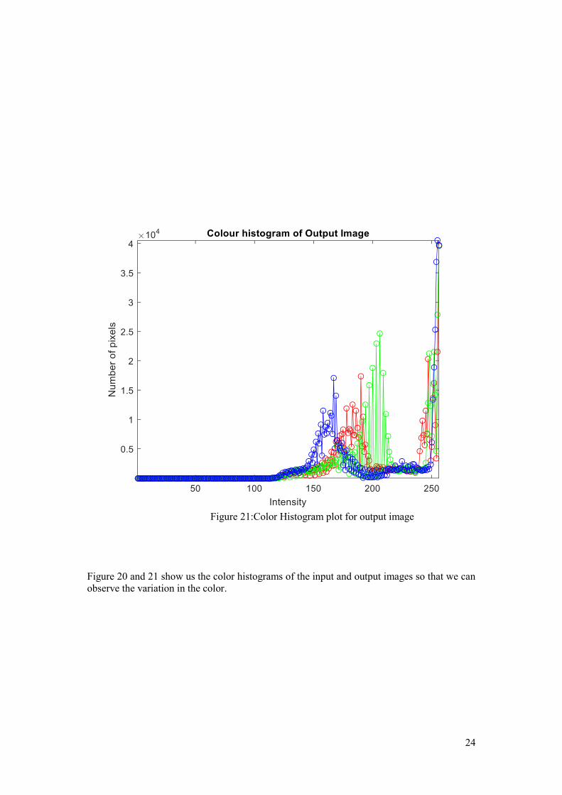
Figure 21:Color Histogram plot for output image

Figure 20 and 21 show us the color histograms of the input and output images so that we can observe the variation in the color.

25

Here we are changing the alpha [10]values and plotting the Output variation for the changed alpha values to 0.25,0.75,1,2.

Figure 22:Output variation for alpha=0.25

Figure 23:Output variation for alpha=0.75

26

Figure 24:Output variation for alpha=1

Figure 25:Output variation for alpha=2

Gamma variation for change in the alpha values is plotted below

27

Figure 26:Gamma variation for change in the alpha values

Figure 26 shows us gamma values for variation of alpha values so that we can easily recognize the best alpha value for gamma.

28

Figure 27:Input Image2

Figure 27 show us the one of our input image which we are going to perform our proposed method.

29

Figure 28: Output image2 after applying TGC

Figure 28 shows the final output of an image after performing our proposed method

Figure 29:Input and Output images are plotted side by side

Input image and the output images are shown side by side to compare them directly in the Figure 29

30

Figure 30:Histogram Plot for both input and output images

Figure 30 shows us the histograms plots of the input and output images and from that we can differentiate the changes in the output by using Median Absolute Deviation(MAD).

31

Figure 31:Color Histogram plot for input image

32

Figure 32:Color Histogram plot for output image

Figure 31 and 32 show us the color histograms of the input and output images so that we can observe the variation in the color. Here we are changing the alpha [10] values and plotting the Output variation for the changed alpha values to 0.25,0.75,1,2.

33

Figure 33:Output variation for alpha=0.25

Figure 34:Output variation for alpha=0.75

34

Figure 35:Output variation for alpha=1

Figure 36:Output variation for alpha=2

35

Figure 37:Gamma variation for change in the alpha values

Figure 37 shows us gamma values for variation of alpha values so that we can easily recognize the best alpha value for gamma.

36

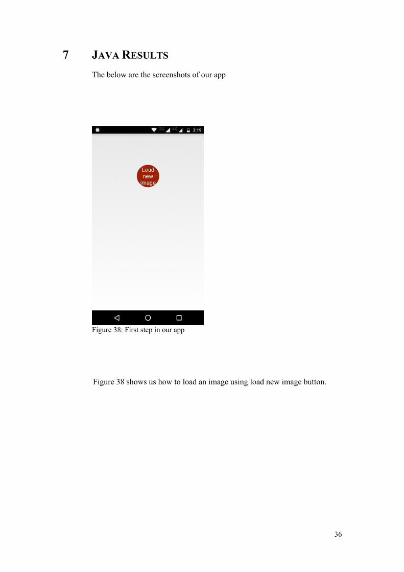
7 JAVA RESULTS The below are the screenshots of our app

Figure 38: First step in our app Figure 38 shows us how to load an image using load new image button.

37

Figure 39:Second step after loading image

Figure 39 shows us modifying image button after loading image

38

Figure 40:Third step after clicking modify image

Figure 40 shows us the action TGC popup button after pressing modify

image button. After pressing Action TGC button we can see the changes in the below Figure 42.

39

Figure 41: Input Camp Fire image to the Application

Figure 42: Output of the Camp fire image in this application Comparing the Output and the input of our application we observe change in the upper 10% of the image only.

40

k pdf PDFw1 cdf 0 2 1801.6543 0

1 17 1802.6543 9.06E-05

2 36 1803.6543 2.58E-04

3 60 1804.6543 5.08E-04

4 97 1805.6543 8.69E-04

5 129 1806.6543 0.001319

6 233 1807.6543 0.002023

7 360 1808.6543 0.003001

8 712 1809.6543 0.004636

9 1295 1810.6543 0.007198

10 2046 1811.6543 0.010811

11 2966 1812.6543 0.015584

12 3081 1813.6543 0.020497

13 3239 1814.6543 0.025596

14 3670 1815.6543 0.031198

15 4021 1816.6543 0.037196

16 3728 1817.6543 0.042864

17 3647 1818.6543 0.048438

18 3256 1819.6543 0.053558

19 3192 1820.6543 0.058603

20 2945 1821.6543 0.063351

21 3074 1822.6543 0.068255

22 2821 1823.6543 0.072852

23 3039 1824.6543 0.077714

24 3114 1825.6543 0.082665

25 3047 1826.6543 0.087537

26 2987 1827.6543 0.092336

27 3037 1828.6543 0.097195

28 2942 1829.6543 0.10194

29 2438 1830.6543 0.106061

30 2426 1831.6543 0.110166

31 2409 1832.6543 0.11425

32 2387 1833.6543 0.118306

33 2267 1834.6543 0.122207

34 2505 1835.6543 0.126413

35 2373 1836.6543 0.130451

36 2555 1837.6543 0.134719

37 2570 1838.6543 0.139006

38 2446 1839.6543 0.143137

39 2603 1840.6543 0.147465

40 2592 1841.6543 0.151779

41 2684 1842.6543 0.156208

42 2893 1843.6543 0.160894

43 3014 1844.6543 0.165725

44 3379 1845.6543 0.17099

41

45 3502 1846.6543 0.176397

46 3888 1847.6543 0.182246

47 4292 1848.6543 0.188546

48 5058 1849.6543 0.195671

49 5651 1850.6543 0.203415

50 6410 1851.6543 0.211926

51 7249 1852.6543 0.22126

52 8165 1853.6543 0.231466

53 8868 1854.6543 0.242324

54 9802 1855.6543 0.254029

55 10162 1856.6543 0.266055

56 10410 1857.6543 0.278301

57 10548 1858.6543 0.290668

58 10798 1859.6543 0.303254

59 10759 1860.6543 0.315807

60 10210 1861.6543 0.327875

61 9506 1862.6543 0.339314

62 9259 1863.6543 0.35053

63 8240 1864.6543 0.360805

64 7712 1865.6543 0.370583

65 7244 1866.6543 0.379913

66 6871 1867.6543 0.388879

67 6713 1868.6543 0.397691

68 6434 1869.6543 0.406226

69 6115 1870.6543 0.414442

70 5999 1871.6543 0.42254

71 5517 1872.6543 0.430145

72 5084 1873.6543 0.437298

73 4718 1874.6543 0.444061

74 4275 1875.6543 0.450342

75 3858 1876.6543 0.456157

76 3728 1877.6543 0.461825

77 3532 1878.6543 0.467267

78 3374 1879.6543 0.472525

79 3079 1880.6543 0.477435

80 3148 1881.6543 0.482427

81 2980 1882.6543 0.487218

82 3074 1883.6543 0.492121

83 3110 1884.6543 0.497068

84 2947 1885.6543 0.501819

85 2876 1886.6543 0.506484

86 3000 1887.6543 0.511299

87 2942 1888.6543 0.516043

88 2900 1889.6543 0.520737

89 2881 1890.6543 0.525408

90 2747 1891.6543 0.529915

42

91 2591 1892.6543 0.534228

92 2661 1893.6543 0.538628

93 2565 1894.6543 0.542909

94 2398 1895.6543 0.546979

95 2366 1896.6543 0.551008

96 2361 1897.6543 0.55503

97 2234 1898.6543 0.558889

98 2284 1899.6543 0.562813

99 2211 1900.6543 0.566642

100 2141 1901.6543 0.57038

101 2187 1902.6543 0.574178

102 1998 1903.6543 0.577727

103 2000 1904.6543 0.581278

104 1863 1905.6543 0.584645

105 1907 1906.6543 0.588072

106 1831 1907.6543 0.591396

107 1796 1908.6543 0.594671

108 1688 1909.6543 0.597798

109 1626 1910.6543 0.600838

110 1679 1911.6543 0.603953

111 1659 1912.6543 0.607039

112 1578 1913.6543 0.610011

113 1541 1914.6543 0.612932

114 1457 1915.6543 0.615731

115 1424 1916.6543 0.618483

116 1432 1917.6543 0.621247

117 1352 1918.6543 0.623893

118 1323 1919.6543 0.626497

119 1321 1920.6543 0.629098

120 1262 1921.6543 0.631611

121 1254 1922.6543 0.634113

122 1137 1923.6543 0.636436

123 1106 1924.6543 0.638713

124 1073 1925.6543 0.640937

125 992 1926.6543 0.643035

126 1067 1927.6543 0.64525

127 1063 1928.6543 0.647459

128 938 1929.6543 0.64947

129 944 1930.6543 0.651491

130 887 1931.6543 0.653419

131 824 1932.6543 0.655244

132 852 1933.6543 0.657114

133 815 1934.6543 0.658924

134 838 1935.6543 0.660771

135 730 1936.6543 0.662437

136 752 1937.6543 0.66414

43

137 678 1938.6543 0.665716

138 665 1939.6543 0.667268

139 672 1940.6543 0.668833

140 660 1941.6543 0.670377

141 605 1942.6543 0.671823

142 588 1943.6543 0.673239

143 580 1944.6543 0.67464

144 593 1945.6543 0.676064

145 613 1946.6543 0.677524

146 593 1947.6543 0.678949

147 519 1948.6543 0.680237

148 588 1949.6543 0.681653

149 574 1950.6543 0.683043

150 611 1951.6543 0.6845

151 566 1952.6543 0.685875

152 554 1953.6543 0.687228

153 581 1954.6543 0.688631

154 484 1955.6543 0.689853

155 540 1956.6543 0.691181

156 582 1957.6543 0.692585

157 629 1958.6543 0.694074

158 580 1959.6543 0.695475

159 583 1960.6543 0.696882

160 555 1961.6543 0.698237

161 567 1962.6543 0.699614

162 506 1963.6543 0.700878

163 465 1964.6543 0.702064

164 497 1965.6543 0.703311

165 406 1966.6543 0.704382

166 428 1967.6543 0.705497

167 377 1968.6543 0.706509

168 368 1969.6543 0.707504

169 376 1970.6543 0.708514

170 357 1971.6543 0.709486

171 309 1972.6543 0.710358

172 321 1973.6543 0.711255

173 330 1974.6543 0.712171

174 318 1975.6543 0.713062

175 283 1976.6543 0.713877

176 310 1977.6543 0.714751

177 310 1978.6543 0.715625

178 291 1979.6543 0.716458

179 297 1980.6543 0.717303

180 301 1981.6543 0.718158

181 341 1982.6543 0.719097

182 321 1983.6543 0.719994

44

183 321 1984.6543 0.720891

184 309 1985.6543 0.721763

185 314 1986.6543 0.722645

186 298 1987.6543 0.723493

187 284 1988.6543 0.724311

188 294 1989.6543 0.72515

189 337 1990.6543 0.726081

190 297 1991.6543 0.726926

191 325 1992.6543 0.727832

192 339 1993.6543 0.728767

193 352 1994.6543 0.729728

194 334 1995.6543 0.730653

195 337 1996.6543 0.731583

196 381 1997.6543 0.732604

197 410 1998.6543 0.733683

198 432 1999.6543 0.734805

199 485 2000.6543 0.736029

200 557 2001.6543 0.737388

201 802 2002.6543 0.739176

202 903 2003.6543 0.74113

203 1412 2004.6543 0.743865

204 1827 2005.6543 0.747183

205 1983 2006.6543 0.750711

206 2369 2007.6543 0.754744

207 2664 2008.6543 0.759148

208 3284 2009.6543 0.764301

209 3962 2010.6543 0.770234

210 5458 2011.6543 0.777778

211 7049 2012.6543 0.786918

212 8308 2013.6543 0.797258

213 9642 2014.6543 0.808819

214 10663 2015.6543 0.821287

215 11636 2016.6543 0.8346

216 11233 2017.6543 0.847564

217 9440 2018.6543 0.858944

218 8281 2019.6543 0.869258

219 6373 2020.6543 0.877732

220 5228 2021.6543 0.885037

221 4226 2022.6543 0.891263

222 3621 2023.6543 0.896808

223 3520 2024.6543 0.902237

224 3447 2025.6543 0.907581

225 3227 2026.6543 0.912666

226 3135 2027.6543 0.917643

227 3191 2028.6543 0.922686

228 3636 2029.6543 0.928248

45

229 3842 2030.6543 0.934045

230 4332 2031.6543 0.940388

231 4295 2032.6543 0.946691

232 3663 2033.6543 0.952284

233 3549 2034.6543 0.957746

234 4181 2035.6543 0.963923

235 3785 2036.6543 0.969655

236 3546 2037.6543 0.975114

237 2308 2038.6543 0.979068

238 1284 2039.6543 0.981614

239 1161 2040.6543 0.983975

240 415 2041.6543 0.985064

241 353 2042.6543 0.986027

242 306 2043.6543 0.986893

243 198 2044.6543 0.987515

244 207 2045.6543 0.988159

245 194 2046.6543 0.988772

246 181 2047.6543 0.989354

247 160 2048.6543 0.989883

248 174 2049.6543 0.990448

249 216 2050.6543 0.991113

250 181 2051.6543 0.991694

251 176 2052.6543 0.992263

252 185 2053.6543 0.992855

253 183 2054.6543 0.993441

254 154 2055.6543 0.993956

255 1156 2056.6543 0.996308 Table 2: Values of k, pdf, PDFw1, cdf for campfire image From the above table, we can observe the k (number of pixels), pdf (probability density function), PDFw1(weights of probability density function), cdf (cumulative distribution function) values of the camp fire image. By observing them we can find the change in the output image cdf values increases and decreases per the pixel values. Here the hsvpixels length of a campfire image is 655560, The maximum value is 1.0,

pdf PDFw1 cdf gamma

Length 256 256 256 256

Minimum value 2 0 0 0.003692

Maximum value

11636 0.01775 0.996308 1

Table 3: Length, Minimum and Maximum Values of pdf, PDFw1, cdf, gamma

46

We had applied our technique on various images and by changing the alpha values to 0.25, 0.75, 2 The output of two images (camp fire and deer images) after changing the alpha values are shown below Alpha = 0.25

Figure 43 : Campfire image when alpha is 0.25

47

Figure 44 : Deer image when alpha is 0.25 Alpha = 0.75

Figure 45 : Campfire image when alpha is 0.75

48

Figure 46 : Deer image when alpha is 0.75 Alpha = 2

Figure 47 : Campfire image when alpha is 2

49

Figure 48 : Deer image when alpha is 2 By observing the output, we conclude that the changes are better in alpha = 0.75 These outputs are taken as a screen shots from Moto G4 plus mobile version 7.0 And also we run this application on HTC desire 820 version 4.2.

50

8 SUMMARY AND CONCLUSION

In this paper, we present a novel enhancement method for enhancing the contrast of an image. This method mainly consists of 5 major steps. In the first step we convert the RGB image into HSV. In the Second step, third plane (V-plane) extraction of HSV image is being done. In the Third step the Weighted Cumulative distribution function is calculated by using Probability distribution function and Probability distribution function is calculated by adjustment parameter alpha. These all steps are done to perform the histogram modification process, when we are performing Probability distribution function the image is equally distributed which is nothing but Histogram Equalization. In the fourth step the Transformed Based gamma correction is performed by Re-shaping the V-plane with gamma value, the gamma value is calculated by Cumulative distributive function. In the Final step the Re-Shaped V-plane is stored in the HSV image then HSV image is converted into RGB image, and the contrast enhanced image is plotted. Here we are performing TGC to Histogram Equalized image this process is known as Variants of Histogram Equalization. We calculate our result on the basis of median absolute deviation value, that is to measure the output variation with respective to the input.

We converted our proposed method into an android application. We succeeded in enhancing the contrast of an image by using our method and we have tested for different alpha values and graphs are respectively plotted. According to our analysis for the given input we get the efficient output by comparing both input and output images. The application is working on Moto G4 Plus version 7.0 and HTC desire 820 version 4.2.

In future, our proposed method can be implemented in video processing. In video, there are number of frames, our method should be applied to each frame individually and the contrast must be enhanced in each frame. All the frames are combined to get a video sequence. The major factor in video processing is execution time, so the execution time must be less for the best method.

51

9 REFERENCE: [1] J. A. Ojo, I. D. Solomon, and S. A. Adeniran, “Contrast enhancement algorithm for

colour images,” in Science and Information Conference (SAI), 2015, 2015, pp. 555–559.

[2] M. M. Ahmed, J. M. Zain, and M. M. Ahmed, “A Study on the Validation of Histogram Equalization as a Contrast Enhancement Technique,” in 2012 International Conference on Advanced Computer Science Applications and Technologies (ACSAT), 2012, pp. 253–256.

[3] C. Y. Wu, J. J. Leou, and C. Hsuan-Ying, “Visual attention region determination using low-level features,” in 2009 IEEE International Symposium on Circuits and Systems, 2009, pp. 3178–3181.

[4] D. Menotti, L. Najman, A. de A. Araujo, and J. Facon, “A Fast Hue-Preserving Histogram Equalization Method for Color Image Enhancement using a Bayesian Framework,” in 14th International Workshop on Systems, Signals and Image Processing, 2007 and 6th EURASIP Conference focused on Speech and Image Processing, Multimedia Communications and Services, 2007, pp. 414–417.

[5] J. H. Han, S. Yang, and B. U. Lee, “A Novel 3-D Color Histogram Equalization Method With Uniform 1-D Gray Scale Histogram,” IEEE Trans. Image Process., vol. 20, no. 2, pp. 506–512, Feb. 2011.

[6] S. C. Huang, F. C. Cheng, and Y. S. Chiu, “Efficient Contrast Enhancement Using Adaptive Gamma Correction With Weighting Distribution,” IEEE Trans. Image Process., vol. 22, no. 3, pp. 1032–1041, Mar. 2013.

[7] “REVIEW OF VARIOUS IMAGE CONTRAST ENHANCEMENT TECHNIQUES.” [Online]. Available: https://www.academia.edu/5540646/REVIEW_OF_VARIOUS_IMAGE_CONTRAST_ENHANCEMENT_TECHNIQUES. [Accessed: 17-Sep-2016].

[8] “CGSD - Gamma Correction Explained.” [Online]. Available: http://www.cgsd.com/papers/gamma_intro.html. [Accessed: 16-Sep-2016].

[9] “A COMPARISON OF HISTOGRAM EQUALIZATION METHOD AND HISTOGRAM EXPANSION.” [Online]. Available: https://www.academia.edu/6481822/A_COMPARISON_OF_HISTOGRAM_EQUALIZATION_METHOD_AND_HISTOGRAM_EXPANSION. [Accessed: 17-Sep-2016].

[10] M. Kim and M. G. Chung, “Recursively separated and weighted histogram equalization for brightness preservation and contrast enhancement,” IEEE Trans. Consum. Electron., vol. 54, no. 3, pp. 1389–1397, Aug. 2008.

52

APPENDIX MATLAB Implementation

close all;

clear all;

clc;

[f,p]=uigetfile('.jpg');

I=strcat(p,f);

img=imread(I);

figure,imshow(img);

title('Input Image','color','Red');

[r,c,~] = size(img);

i=img;

%%%%%%%%%%%%%RGB to HSV conversion%%%%%%%%%%%%%%%%%%

HSV = rgb2hsv(i);

% figure,imshow(HSV);

% title('HSV Image','color','Green');

%%%%%%%%%%%%%Third plane extraction of HSV Image%%%%

V = HSV(:,:,3);

% figure,imshow(V);

% title('Third plane of HSV image','color','Blue');

%%%%Probability Density Function Calculation%%%%%%%%

%pdf:Probability Density Function%%%%%%%%%%%%%%%%%%%

[counts, x] = imhist(V);

pdf = counts/(sum(counts));

% alph: adjusted parameter

alph = 0.75;

% --- Weighting Distribution -----

pdf_max = max(pdf);

pdf_min = min(pdf);

pdf_w = pdf_max*((pdf - pdf_min)./(pdf_max -

pdf_min)).^alph;

% --- weighted cdf -----

% lmax: maximum intensity of input

lmax_idx = (find(counts, 1, 'last'));

lmax = max(V(:));

sum_pdf_w = 0;

all_pdf_w = sum(pdf_w);

for i=1:lmax_idx

sum_pdf_w = sum_pdf_w + pdf_w(i);

cdf_w(i) = sum_pdf_w./all_pdf_w;

end

gamma = 1-cdf_w;

% ---- Enhancement ----

V = reshape(V,r*c,1);

T = zeros(size(V));

for i=1:lmax_idx

L = V(V==x(i));

53

T(V==x(i)) = lmax*(L./lmax).^gamma(i);

end

V2 = reshape(T,r,c);

hsv_image(:,:,3) = V2;

hsv_image(:,:,2) = HSV(:,:,2);

hsv_image(:,:,1) = HSV(:,:,1);

im_out = hsv2rgb(hsv_image);

im_out = uint8(im_out*255);

%Contrasted enhanced image

figure,imshow(im_out);

title('Output Image for alpha = 0.75','color','Blue');

% figure,imshowpair(img,im_out,'montage');

% title('input mage

output image')

% d=gampdf(gamma,1);

% figure,plot(d);

% xlabel('intensity');

% ylabel('gamma')

compareimq(img,im_out);

%%Code for compareimq(img,im_out)

% function [] = compareimq(img1, img2)

% Compares histogram and MAD of two images of the same

size and type. This

% is an extension of a file compare.m written by Marcus

Rodan as part of

% ET2584 during summer 2016.

% Ver 1.1 2016-07-18. Still under development. Benny L.

function [] = compareimq(img1, img2)

s = size(img1);

figure(10)

subplot(2,2,1);

imshow(img1);

title('Image 1');

subplot(2,2,2);

imshow(img2);

title('Image 2');

figure

if length(s) == 3

hsvimg1 = rgb2hsv(img1);

vimg1 = hsvimg1(:,:,3); % Select only intensity

of image

mad = median(abs(vimg1(:)-median(vimg1(:))));

imhist(vimg1);

xlabel('Intensity');

ylabel('Number of pixels')

title(['Histogram of Input Image. MAD='

num2str(mad,2)]);

figure

hsvimg2 = rgb2hsv(img2);

54

vimg2 = hsvimg2(:,:,3); % Select only intensity

of image

mad = median(abs(vimg2(:)-median(vimg2(:))));

imhist(hsvimg2(:,:,3));

xlabel('Intensity');

ylabel('Number of pixels')

title(['Histogram of Output Image . MAD='

num2str(mad,2)]);

showcolorhist(img1,101);title('Colour histogram of

Input Image')

xlabel('Intensity');

ylabel('Number of pixels')

showcolorhist(img2,102);title('Colour histogram of

Output Image')

xlabel('Intensity');

ylabel('Number of pixels')

else

img1 = double(img1);

img1 = img1/max(img1(:));

mad = median(abs(img1(:)-median(img1(:))))

imhist(img1);

title(['Histogram of Input Image . MAD='

num2str(mad,2)]);

subplot(2,2,4);

img2 = double(img2);

img2 = img2/max(img2(:));

mad = median(abs(img2(:)-median(img2(:))));

imhist(img2);

title(['Histogram of Output Image. MAD='

num2str(mad,2)]);

end

end