Contracts and Technology Adoption

(Article begins on next page)

The Harvard community has made this article openly available.Please share how this access benefits you. Your story matters.

Citation Acemoglu, Daron, Pol Antras, and Elhanan Helpman. 2007.Contracts and technology adoption. American Economic Review97(3): 916-943.

Published Version doi:10.1257/aer.97.3.916

Accessed June 23, 2018 7:37:44 AM EDT

Citable Link http://nrs.harvard.edu/urn-3:HUL.InstRepos:3199063

Terms of Use This article was downloaded from Harvard University's DASHrepository, and is made available under the terms and conditionsapplicable to Other Posted Material, as set forth athttp://nrs.harvard.edu/urn-3:HUL.InstRepos:dash.current.terms-of-use#LAA

Contracts and Technology Adoption�

Daron AcemogluDepartment of Economics, MIT

Pol AntràsDepartment of Economics, Harvard University

Elhanan HelpmanDepartment of Economics, Harvard University

November 28, 2006

Abstract

We develop a tractable framework for the analysis of the relationship between contractual

incompleteness, technological complementarities, and technology adoption. In our model a �rm

chooses its technology and investment levels in contractible activities by suppliers of intermediate

inputs. Suppliers then choose investments in noncontractible activities, anticipating payo¤s

from an ex post bargaining game. We show that greater contractual incompleteness leads to the

adoption of less advanced technologies and that the impact of contractual incompleteness is more

pronounced when there is greater complementary among the intermediate inputs. We study a

number of applications of the main framework and show that the mechanism proposed in the

paper can generate sizable productivity di¤erences across countries with di¤erent contracting

institutions and that di¤erences in contracting institutions lead to endogenous comparative

advantage di¤erences.

Keywords: comparative advantage, economic growth, incomplete contracts, technologychoice, theory of the �rm.

JEL Classi�cation: D23, F10, L23, O30.

�A previous version of this paper was circulated under the title �Contracts and the Division of Labor.� Wethank Gene Grossman, Oliver Hart, Kalina Manova, Damián Migueles, Giacomo Ponzetto, Richard Rogerson, RaniSpiegler, two anonymous referees, and participants in the Canadian Institute for Advanced Research and MinnesotaWorkshop in Macroeconomic Theory conferences, and seminar participants at Harvard, MIT, Tel Aviv, UniversitatPompeu Fabra, Houston, UCSD, Southern Methodist, Stockholm School of Economics, Stockholm University (IIES),ECARES, Colorado-Boulder, Kellogg, NYU, UBC, Georgetown, World Bank, Montreal, Brandeis, Wisconsin, UCBerkeley, Haifa, Syracuse, and Autònoma-Barcelona for useful comments. We also thank Davin Chor, Alexandre Debsand Ran Melamed for excellent research assistance. Acemoglu and Helpman thank the National Science Foundationfor �nancial support. Much of Helpman�s work for this paper was done when he was Sackler Visiting Professor atTel Aviv University.

1 Introduction

There is widespread agreement that di¤erences in technology are a major source of productivity

di¤erences across �rms, industries and nations.1 Despite this widespread agreement, we are far from

an established framework for the analysis of technology choices of �rms. In this paper, we take a

step in this direction and develop a simple model to study the impact of contracting institutions,

which regulate the relationship between the �rm and its suppliers, on technology choices.

Our model combines two well-established approaches. The �rst is the representation of tech-

nology as the range of intermediate inputs used by �rms; a greater range of intermediate inputs

increases productivity by allowing greater specialization and thus corresponds to more �advanced�

technology.2 The second is Grossman and Hart�s (1986) and Hart and Moore�s (1990) approach to

incomplete-contracting models of the �rm. We study technology choice of �rms under incomplete

contracts, and extend Hart and Moore�s framework, by allowing contracts to be partially incom-

plete. This combination enables us to investigate how the degree of contractual incompleteness

and the extent of technological complementarities between intermediate inputs a¤ect the choice of

technology.

In our baseline model a �rm decides on technology (on the range of specialized intermediate

goods), recognizing that a more advanced technology is more productive, but also entails a variety

of costs. In addition to the direct pecuniary costs of engaging more suppliers (corresponding to

the greater range of intermediate inputs), a more advanced technology necessitates contracting

with more suppliers. All of the activities that suppliers undertake are relationship-speci�c, and a

fraction of those is ex ante contractible, while the rest, as in the work by Grossman-Hart-Moore,

are nonveri�able and noncontractible. The fraction of contractible activities is our measure of the

quality of contracting institutions.3 Suppliers are contractually obliged to perform their duties in

the contractible activities, but they are free to choose their investments in noncontractible activities

and to withhold their services in these activities from the �rm. This combination of noncontractible

investments and relationship-speci�city leads to an ex post multilateral bargaining problem. As

in Hart and Moore (1990), we use the Shapley value to determine the division of ex post surplus

between the �rm and its suppliers. We derive an explicit solution for this division of surplus, which

enables us to develop a simple characterization of the equilibrium.

A supplier�s expected payo¤ in the bargaining game determines her willingness to invest in the

noncontractible activities. Since she is not the full residual claimant of the output gains derived from

1Among others, see Klenow and Rodriguez (1997), Hall and Jones (1999) or Caselli (2004) for countries, andKlette (1996), Griliches (1998), Sutton (1998) or Klette and Kortum (2004) for �rms.

2See, among others, Ethier (1982), Romer (1990) and Grossman and Helpman (1991) for previous uses of thisrepresentation. See also the textbook treatment in Barro and Sala-i-Martin (2003). There is a natural relationshipbetween this view of technology and the division of labor within a �rm. We investigated this link in the earlier versionof the current paper, Acemoglu, Antràs and Helpman (2005), and do not elaborate on it here.

3Maskin and Tirole (1999) question whether the presence of nonveri�able actions and unforeseen contingenciesnecessarily lead to incomplete contracts. Their argument is not central to our analysis because it assumes the presenceof �strong�contracting institutions (which, for example, allow contracts to specify sophisticated mechanisms), whilein our model a fraction of activities may be noncontractible not because of �technological� reasons but because ofweak contracting institutions.

1

her investments, she tends to underinvest. Greater contractual incompleteness thus reduces supplier

investments, making more advanced technologies less pro�table. Furthermore, a greater degree of

technological complementarity reduces the incentive to choose more advanced technologies; though

greater technological complementarity increases equilibrium ex post payo¤s to every supplier, it also

makes their payo¤s less sensitive to their noncontractible investments, discouraging investments

and, via this channel, depressing the pro�tability of more advanced technologies.

An advantage of our framework is its relative tractability. The equilibrium of our model can be

represented by a reduced-form pro�t function for �rms given by

AZF (N)� C (N)� w0N; (1)

where N represents the technology level,C (N) is the cost of technology N , A is a measure of

aggregate demand or the scale of the market, and w0N corresponds to the value of the N suppliers�

outside options. F (N) is an increasing function that captures the positive e¤ect of choosing more

advanced technologies on revenue. The e¤ects of contractual incompleteness and technological

complementarity are summarized by the variable Z. This variable a¤ects productivity and is

decreasing in the degree of contract incompleteness and technological complementarity. Moreover,

the elasticity of Z with respect to the quality of contracting institutions is higher when there is

greater complementarity between intermediate inputs. This last result has important implications

for equilibrium industry structure and the patterns of comparative advantage, because it implies

that sectors (�rms) with greater complementarities between inputs are more �contract dependent�.

We use this framework to show that the combination of contractual imperfections and tech-

nology choice (or adoption) may have important implications for cross-country income di¤erences,

equilibrium organizational forms, and patterns of international specialization and trade.

First, we show that our baseline model can generate sizable di¤erences in productivity from

di¤erences in the quality of contracting institutions. In particular, using a range of reasonable values

for the key parameters of the model, we �nd that when the degree of technological complementarity

is su¢ ciently high, relatively modest changes in the fraction of activities that are contractible can

lead to large changes in productivity.

Second, we derive a range of implications about the equilibrium organizational form. Our results

here show that the combination of weak contracting institutions and credit market imperfections

may encourage greater vertical integration.

Third, we present a number of general equilibrium applications of this framework. The general

equilibrium interactions result from the fact that an improvement in contracting institutions does

not increase the choice of technology in all sectors (�rms). Instead, more advanced technologies are

chosen in the more contract-dependent sectors. We show that in the context of an open economy,

this feature leads to an endogenous structure of comparative advantage. In particular, among

countries with identical technological opportunities (production possibility sets), those with better

contracting institutions specialize in sectors with greater complementarities among inputs. These

predictions are consistent with the recent empirical results presented in Nunn (2005) and Levchenko

2

(2003).

As mentioned above, our work is related to two strands of the literature. The �rst investigates

the determinants of �rm-level technology (including the division of labor) and includes, among

others, Becker and Murphy (1992) and Yang and Borland (1991) on the impact of the extent

of the market on the division of labor and Romer (1990) and Grossman and Helpman (1991)

on endogenous technological change. None of these studies investigate the e¤ects of contracting

institutions on technology choice. The second literature deals with the internal organization of the

�rm. It includes the papers by Grossman-Hart-Moore discussed above, as well as Klein, Crawford

and Alchian (1978) and Williamson (1975, 1985), who emphasize incomplete contracts and hold-up

problems. Here, the papers by Stole and Zwiebel (1996a,b) and Bakos and Brynjolfsson (1993) are

most closely related to ours. Stole and Zwiebel consider a relationship between a �rm and a number

of workers whose wages are determined by ex post bargaining according to the Shapley value. They

show how the �rm may overemploy in order to reduce the bargaining power of the workers and

discuss the implications of this framework for a number of organizational design issues. Stole and

Zwiebel�s framework does not have relationship-speci�c investments, however, which is at the core

of our approach, and they do not discuss the e¤ects of the degree of contractual incompleteness

and the degree of complementarity between inputs on the equilibrium technology choice.4

Finally, our paper is also related to the literature on the macroeconomic implications of contrac-

tual imperfections. A number of papers, most notably Quintin (2001), Amaral and Quintin (2005),

Erosa and Hidalgo (2005) and Castro, Clementi and MacDonald (2004), investigate the quanti-

tative impact of contractual and capital market imperfections on aggregate productivity.5 Our

approach di¤ers from these papers since we focus on technology choice and relationship-speci�c

investments, and because we develop a tractable framework that can be applied in a range of prob-

lems. Although we do not undertake a detailed calibration exercise as in these papers, the results

in subsection 5.1 suggest that the economic mechanism developed in this paper can lead to quanti-

tatively large e¤ects. Finally, Levchenko (2003), Costinot (2004), Nunn (2005) and Antràs (2005)

also generate endogenous comparative advantage across countries from di¤erences in contractual

environments. Among these papers, Costinot (2004) is most closely related, since he also develops

a model of endogenous comparative advantage based on specialization, though his approach is more

reduced-form than our model.

The rest of the paper is organized as follows. Section 2 introduces the basic environment.

Section 3 characterizes the equilibrium with complete contracts. Section 4 introduces incomplete

contracts into the framework of Section 2, characterizes the equilibrium, and derives the major

comparative static results. Section 5 considers a number of applications of our basic framework.

Section 6 concludes. Proofs of the main results are provided in the Appendix.

4Another related paper is Blanchard and Kremer (1997), which studies the impact of ine¢ cient sequential con-tracting between a �rm and its suppliers in a model where output is a Leontief aggregate of the inputs of thesuppliers.

5Acemoglu and Zilibotti (1999), Martimort and Verdier (2000, 2004) and Francois and Roberts (2003) study thequalitative impact of changes in the internal organization of �rms on economic growth.

3

2 Technology and Payo¤s

Consider a pro�t-maximizing �rm facing a demand function q = Ap�1=(1��) for its �nal product,

where q denotes quantity and p denotes price. The parameter � 2 (0; 1) determines the elasticityof demand while A > 0 determines the level of demand or the �market size�. The �rm treats the

demand level A as exogenous. This form of demand can be derived from a constant elasticity of

substitution preference structure for di¤erentiated products (see Section 5.3) and it generates a

revenue function

R = A1��q� : (2)

Production depends on the technology choice of the �rm. More advanced (more productive)

technologies involve a greater range of intermediate goods and thus a higher degree of specialization.

The technology level of the �rm is denoted by N 2 R+ and for each j 2 [0; N ], X (j) is the quantityof intermediate input j. Given technology N , the production function of the �rm is

q = N�+1�1=��Z N

0X (j)� dj

�1=�, 0 < � < 1; � > 0: (3)

A number of features of this production function are worth noting. First, � determines the degree

of complementarity between inputs; since � 2 (0; 1), the elasticity of substitution between them,1= (1� �), is always greater than one. Second, we follow Benassy (1998) in introducing the termN�+1�1=� in front of the integral, which allows us to separately control the elasticity of substitution

between inputs and the elasticity of output with respect to the level of the technology. To see this,

consider the case where X (j) = X for all j. Then the output of technology N is q = N�+1X.

Consequently, both output and productivity (de�ned as either q= (NX) or q=N) are independent

of � and depend positively on N , with elasticity determined by the parameter �.6

There is a large number of pro�t-maximizing suppliers that can produce the necessary inter-

mediate goods, each with the same outside option w0. For now, w0 is taken as given, but it will

be endogenized in Section 5.3. We assume that each intermediate input needs to be produced by

a di¤erent supplier with whom the �rm needs to contract.7

A supplier assigned to the production of an intermediate input needs to undertake relationship-

speci�c investments in a unit measure of (symmetric) activities. There is a constant marginal cost

of investment cx for each activity.8 The production function of intermediate inputs is Cobb-Douglas

and symmetric in the activities:

X (j) = exp

�Z 1

0lnx (i; j) di

�, (4)

6 In contrast, with the standard speci�cation of the CES production function, without the term N�+1�1=� in front(i.e., � = 1=�� 1), total output is q = N1=�X, and the two elasticities are governed by the same parameter, �.

7A previous version of the paper, Acemoglu, Antràs and Helpman (2005), also endogenized the allocation of inputsto suppliers using an augmented model with additional diseconomies of scope.

8One can think of cx as the marginal cost of e¤ort; see the formulation of this e¤ort in utility terms in Section 5.3.

4

where x (i; j) is the level of investment in activity i performed by the supplier of input j. This formu-

lation will allow a tractable parameterization of contractual incompleteness in Section 4, whereby a

subset of the investments necessary for production will be nonveri�able and thus noncontractible.

Finally, we assume that adopting (and using) a technology N involves costs C (N), and impose

Assumption 1

(i) For all N > 0, C (N) is twice continuously di¤erentiable, with C 0 (N) > 0 and C 00 (N) � 0.

(ii) For all N > 0, NC 00 (N) = [C 0 (N) + w0] > [� (�+ 1)� 1] = (1� �).

The �rst part of this assumption is standard; costs are increasing and convex. The second part

will ensure a �nite and positive choice of N .

Let the payment to supplier j consist of two parts: an ex ante payment � (j) 2 R before theinvestment levels x (i; j) take place, and a payment s (j) after the investments. Then, the payo¤ to

supplier j, also taking account of her outside option, is

�x (j) = max

�� (j) + s (j)�

Z 1

0cxx (i; j) di; w0

�: (5)

Similarly, the payo¤ to the �rm is

� = R�Z N

0[� (j) + s (j)] dj � C (N) ; (6)

where R is revenue and the other two terms on the right-hand side represent costs. Substituting

(3) and (4) into (2), revenue can be expressed as

R = A1��N�(�+1�1=�)�Z N

0

�exp

�Z 1

0lnx (i; j) di

���dj

��=�. (7)

3 Equilibrium under Complete Contracts

As a benchmark, consider the case of complete contracts (the ��rst best�from the viewpoint of the

�rm). With complete contracts, the �rm has full control over all investments and pays each supplier

her outside option. In analogy to our treatment below of technology adoption under incomplete

contracts, consider a game form where the �rm chooses a technology level N and makes a contract

o¤erhfx (i; j)gi2[0;1] ; fs (j) ; � (j)g

ifor every input j 2 [0; N ]. If a supplier accepts this contract

for input j, she is obliged to supply fx (i; j)gi2[0;1] as stipulated in the contract in exchange forthe payments fs (j) ; � (j)g. A subgame perfect equilibrium of this game is a strategy combination

for the �rm and the suppliers such that suppliers maximize (5) and the �rm maximizes (6). An

equilibrium can be alternatively represented as a solution to the following maximization problem:

maxN;fx(i;j)gi;j ;fs(j);�(j)gj

R�Z N

0[� (j) + s (j)] dj � C (N) (8)

5

subject to (7) and the suppliers�participation constraint,

s (j) + � (j)� cxZ 1

0x (i; j) di � w0 for all j 2 [0; N ] : (9)

Since the �rm has no reason to provide rents to the suppliers, it chooses payments s (j) and � (j)

that satisfy (9) with equality.9 Moreover, since the �rm�s objective function, (8), is (jointly) concave

in the investment levels x (i; j) and these investments are all equally costly, the �rm chooses the

same investment level x for all activities in all intermediate inputs. Now, substituting for (9) in

(8), we obtain the following simpler unconstrained maximization problem for the �rm:

maxN;x

A1��N�(�+1)x� � cxNx� C (N)� w0N: (10)

>From the �rst-order conditions of this problem, we obtain:

(N�)�(�+1)�1

1�� A��1=(1��)c��=(1��)x = C 0 (N�) + w0; (11)

x� =C 0 (N�) + w0

�cx: (12)

Equations (11) and (12) can be solved recursively. Given Assumption 1, equation (11) yields a

unique solution for N�, which, together with (12), yields a unique solution for x�.10

When all the investment levels are identical and equal to x, output equals q = N�+1x. Since

NX = Nx inputs are used in the production process, we can de�ne productivity as output divided

by total input use, P = N�. In the case of complete contracts this productivity level is

P � = (N�)� ; (13)

which is increasing in the level of technology. In the next section we compare this to equilibrium

productivity under incomplete contracts.11

The next proposition describes the key properties of the equilibrium (proof in the Appendix).

Proposition 1 Suppose that Assumption 1 holds. Then with complete contracts there exists aunique equilibrium with technology and investment levels N� > 0 and x� > 0 given by (11) and

(12). Furthermore, this equilibrium satis�es:

@N�

@A> 0;

@x�

@A� 0; @N

�

@�=@x�

@�= 0:

9With complete contracts, � (j) and s (j) are perfect substitutes, so that only the sum s (j) + � (j) matters. Thiswill not be the case when contracts are incomplete.10We show in the Appendix that the second-order conditions are satis�ed under Assumption 1.11This measure of productivity implicitly assumes that all the investments x (i; j) are measured accurately. There

may be some tension between this assumption and the assumption that the cost of these investments is not pecuniary.For this reason in the previous version, we also considered another de�nition of productivity: output divided by thenumber of suppliers, P = q=N = (N)� x. The ranking of productivity levels between complete and incompletecontracts is the same under both de�nitions and the quantitative e¤ects of changes in � on productivity are smallerwith our main de�nition.

6

In the case of complete contracts, the size of the market (as parameterized by the demand level

A) has a positive e¤ect on investments by suppliers of intermediate inputs and productivity. The

other noteworthy implication of this proposition is that under complete contracts, the level of tech-

nology and thus productivity do not depend on the elasticity of substitution between intermediate

inputs, 1= (1� �).

4 Equilibrium under Incomplete Contracts

4.1 Incomplete Contracts

We now consider the same environment under incomplete contracts. We model the imperfection

of the contracting institutions by assuming that there exists a � 2 [0; 1] such that, for every

intermediate input j, investments in activities 0 � i � � are observable and veri�able and thereforecontractible, while investments in activities � < i � 1 are not contractible. Consequently, a

contract stipulates investment levels x (i; j) for the � contractible activities, but does not specify

the investment levels in the remaining 1 � � noncontractible activities. Instead, suppliers choosetheir investments in noncontractible activities in anticipation of the ex post distribution of revenue,

and may decide to withhold their services in these activities from the �rm. We follow the incomplete

contracts literature and assume that the ex post distribution of revenue is governed by multilateral

bargaining, and, as in Hart and Moore (1990), we adopt the Shapley value as the solution concept

for this multilateral bargaining game (more on this below).12

The timing of events is as follows:

� The �rm adopts a technology N and o¤ers a contract [fxc (i; j)g�i=0 ; � (j)] for every interme-diate input j 2 [0; N ], where xc (i; j) is an investment level in a contractible activity and � (j)is an upfront payment to supplier j. The payment � (j) can be positive or negative.

� Potential suppliers decide whether to apply for the contracts. Then the �rm chooses N

suppliers, one for each intermediate input j.

� All suppliers j 2 [0; N ] simultaneously choose investment levels x (i; j) for all i 2 [0; 1]. Inthe contractible activities i 2 [0; �] they invest x (i; j) = xc (i; j).

� The suppliers and the �rm bargain over the division of revenue, and at this stage, suppliers

can withhold their services in noncontractible activities.

� Output is produced and sold, and the revenue R is distributed according to the bargaining

agreement.

We will characterize a symmetric subgame perfect equilibrium (SSPE for short) of this game,

where bargaining outcomes in all subgames are determined by Shapley values.12The incomplete contracts literature also assumes that revenues are noncontractible. As is well known, with

bilateral contracting or with multilateral contracting and a budget breaker (e.g., Holmström, 1982), contracting onrevenues would improve incentives. In our setting, we do not need this assumption, since each �rm has a continuumof suppliers and contracts on total revenues would not provide additional investment incentives to suppliers.

7

4.2 De�nition of Equilibrium and Preliminaries

Behavior along the SSPE can be described by a tuplen~N; ~xc; ~xn; ~�

oin which ~N represents the

level of technology, ~xc the investment in contractible activities, ~xn the investment in noncontractible

activities, and ~� the upfront payment to every supplier. That is, for every j 2h0; ~N

ithe upfront

payment is � (j) = ~� , and the investment levels are x (i; j) = ~xc for i 2 [0; �] and x (i; j) = ~xn for

i 2 (�; 1]. With a slight abuse of terminology, we will denote the SSPE byn~N; ~xc; ~xn

o.

The SSPE can be characterized by backward induction. First, consider the penultimate stage of

the game, with N as the level of technology, xc as the level of investment in contractible activities.

Suppose also that each supplier other than j has chosen a level of investment in noncontractible

activities equal to xn (�j) (these are all the same, because we are constructing a symmetric equilib-rium), while the investment level in every noncontractible activity by supplier j is xn (j).13 Given

these investments, the suppliers and the �rm will engage in multilateral Shapley bargaining. Denote

the Shapley value of supplier j under these circumstances by �sx [N;xc; xn (�j) ; xn (j)]. We derivean explicit formula for this value in the next subsection. For now, note that optimal investment

by supplier j implies that xn (j) is chosen to maximize �sx [N;xc; xn (�j) ; xn (j)] minus the costof investment in noncontractible activities, (1� �) cxxn (j). In a symmetric equilibrium, we needxn (j) = xn (�j), or in other words, xn needs to be a �xed-point given by:14

xn = argmaxxn(j)

�sx [N;xc; xn; xn (j)]� (1� �) cxxn (j) : (14)

Equation (14) can be thought of as an �incentive compatibility constraint,� with the additional

symmetry requirement.

In a symmetric equilibrium with technology N , with investment in contractible activities given

by xc and with investment in noncontractible activities equal to xn, the revenue of the �rm is given

by R = A1���N�+1x�c x

1��n

��. Moreover, let sx (N;xc; xn) = �sx (N;xc; xn; xn), then the Shapley

value of the �rm is obtained as a residual:

sq (N;xc; xn) = A1�� �N�+1x�c x

1��n

�� �Nsx (N;xc; xn) :Now consider the stage in which the �rm chooses N suppliers from a pool of applicants. If

suppliers expect to receive less than their outside option, w0, this pool is empty. Therefore, for pro-

duction to take place, the �nal-good producer has to o¤er a contract that satis�es the participation

constraint of suppliers under incomplete contracts, i.e.,

�sx (N;xc; xn; xn) + � � �cxxc + (1� �) cxxn + w0 for xn that satis�es (14). (15)

13More generally, we would need to consider a distribution of investment levels, fxn (i; j)gi2(�;1] for supplier j,where some of the activities may receive more investment than others. It is straightforward to show, however, thatthe best deviation for a supplier is to choose the same level of investment in all noncontractible activities. For thisreason we save on notation and restrict attention to only such deviations.14This equation should be written with �2� instead of �=�. However, we show below that the �xed point xn in

(14) is unique, justifying our use of �=�.

8

In other words, given N and (xc; �), each supplier j 2 [0; N ] should expect her Shapley value plusthe upfront payment to cover the cost of investment in contractible and noncontractible activities

and the value of her outside option.

The maximization problem of the �rm can then be written as:

maxN;xc;xn;�

sq (N;xc; xn)�N� � C (N) subject to (14) and (15).

With no restrictions on � , the participation constraint (15) will be satis�ed with equality;

otherwise the �rm could reduce � without violating (15) and increase its pro�ts. We can therefore

solve � from this constraint, substitute the solution into the �rm�s objective function and obtain

the simpler maximization problem:15

maxN;xc;xn

sq (N;xc; xn)+N [�sx (N;xc; xn; xn)� �cxxc � (1� �) cxxn]�C (N)�w0N subject to (14).

(16)

The SSPEn~N; ~xc; ~xn

osolves this problem, and the corresponding upfront payment satis�es

~� = �cx~xc + (1� �) cx~xn + w0 � �sx�~N; ~xc; ~xn; ~xn

�: (17)

4.3 Bargaining

We now derive the Shapley values in this game (see Shapley, 1953, or Osborne and Rubinstein,

1994). In a bargaining game with a �nite number of players, each player�s Shapley value is the

average of her contributions to all coalitions that consist of players ordered below her in all feasible

permutations. More explicitly, in a game with M + 1 players, let g = fg (0) ; g (1) ; :::; g (M)g be apermutation of 0; 1; 2; :::;M , where player 0 is the �rm and players 1; 2; :::;M are the suppliers, and

let zjg = fj0 j g (j) > g (j0)g be the set of players ordered below j in the permutation g. We denoteby G the set of feasible permutations and by v : G! R the value of the coalition consisting of anysubset of the M + 1 players.16 Then the Shapley value of player j is

sj =1

(M + 1)!

Xg2G

�v�zjg [ j

�� v

�zjg��:

In the Appendix, we derive the asymptotic Shapley value of Aumann and Shapley (1974), by

considering the limit of this expression as the number of players goes to in�nity.17 Leaving the

formal derivation to the Appendix, here we provide a heuristic derivation of this Shapley value.

Suppose the �rm has adopted technology N , all suppliers provide an amount xc of every con-

15Note that, as in the case with complete contracts, the �rm chooses its technology and investment levels tomaximize sale revenues net of total costs. The key di¤erence is that with incomplete contracts, this maximizationproblem is constrained by the �incentive compatibility�condition (14).16 In our game, the value of a coalition equals the amount of revenue this coalition can generate.17More formally, we divide the interval [0; N ] into M equally spaced subintervals with all the intermediate inputs

in each subinterval of length N=M performed by a single supplier. We then solve for the Shapley value and take thelimit of this solution as M !1. See Aumann and Shapley (1974) or Stole and Zwiebel (1996b).

9

tractible activity, and all suppliers other than j invest xn (�j) in every noncontractible activity,while supplier j invests xn (j). To compute the Shapley value for supplier j, �rst note that the

�rm is an essential player in this bargaining game (if a coalition does not include the �rm, then

its output equals zero regardless of its size). Consequently, the supplier j�s marginal contribution

is equal to zero when a coalition does not include the �rm. When it does include the �rm and a

measure n of suppliers, the marginal contribution of supplier j is m (j; n) = @ �R=@n, where

�R = A1��N�(�+1�1=�)�Z n

0

�exp

�Z 1

0lnx (i; k) di

���dk

��=�is the revenue derived from the employment of n inputs with technology N , and the last input k = n

is provided by supplier j. Since x (i; k) = xc for all 0 � i � � and all 0 � k � n, x (i; k) = xn (�j)for all � < i � 1 and all 0 � k < n, and x (i; k) = xn (j) for all � < i � 1 and k = n, evaluating theprevious expression enables us to write the marginal contribution of supplier j as

m (j; n) =�

�A1��N�(�+1�1=�)

�xn (j)

xn (�j)

�(1��)�x��c xn (�j)

�(1��) n(���)=�. (18)

The Shapley value of supplier j is the average of her marginal contributions to coalitions that

consist of players ordered below her in all feasible orderings. A supplier that has a measure n of

players ordered below her has a marginal contribution of m (j; n) if the �rm is ordered below her

(probability n=N) and 0 otherwise (probability 1� n=N). Averaging over all possible orderings ofthe players and using (18), we obtain:

�sx [N;xc; xn (�j) ; xn (j)] =1

N

Z N

0

� nN

�m (j; n) dn

= (1� )A1���xn (j)

xn (�j)

�(1��)�x��c xn (�j)

�(1��)N�(�+1)�1,

where

� �

�+ �: (19)

We therefore obtain the following lemma (see the Appendix for the formal proof):

Lemma 1 Suppose that supplier j invests xn (j) in her noncontractible activities, all the other sup-pliers invest xn (�j) in their noncontractible activities, every supplier invests xc in her contractibleactivities, and the level of technology is N . Then the Shapley value of supplier j is

�sx [N;xc; xn (�j) ; xn (j)] = (1� )A1���xn (j)

xn (�j)

�(1��)�x��c xn (�j)

�(1��)N�(�+1)�1, (20)

where is de�ned in (19).

A number of features of (20) are worth noting. First, in equilibrium, all suppliers invest equally

10

in all the noncontractible activities, i.e., xn (j) = xn (�j) = xn, and so

sx (N;xc; xn) = �sx (N;xc; xn; xn) = (1� )A1��x��c x�(1��)n N�(�+1)�1 = (1� ) RN; (21)

where R = A1��x��c x�(1��)n N�(�+1) is the total revenue of the �rm. Thus, the joint Shapley value

of the suppliers, Nsx (N;xc; xn), equals the fraction 1� of the revenue, and the �rm receives the

remaining fraction , i.e.,

sq (N;xc; xn) = A1��x��c x

�(1��)n N�(�+1) = R: (22)

This is a relatively simple rule for the division of revenue between the �rm and its suppliers.

Second, the derived parameter � �= (�+ �) represents the bargaining power of the �rm; it isincreasing in � and decreasing in �. A higher elasticity of substitution between intermediate inputs,

i.e., a higher �, raises the �rm�s bargaining power, because it makes every supplier less essential

in production and therefore raises the share of revenue appropriated by the �rm. In contrast, a

higher elasticity of demand for the �nal good, i.e., higher �, reduces the �rm�s bargaining power,

because, for any coalition, it reduces the marginal contribution of the �rm to the coalition�s payo¤

as a fraction of revenue.18

Furthermore, when � is smaller, �sx [N;xc; xn (�j) ; xn (j)] is more concave with respect to xn (j),because greater complementary between the intermediate inputs implies that a given change in the

relative employment of two inputs has a larger impact on their relative marginal products. The

impact of � on the concavity of �sx (�) will play an important role in the following results. Theparameter �, on the other hand, a¤ects the concavity of revenue in output (see (2)) but has no

e¤ect on the concavity of �sx with respect to xn (j), because with a continuum of suppliers, a single

supplier has an in�nitesimal e¤ect on output.

4.4 Equilibrium

To characterize a SSPE, we �rst derive the incentive compatibility constraint using (14) and (20):

xn = argmaxxn(j)

(1� )A1���xn (j)

xn

�(1��)�x��c x

�(1��)n N�(�+1)�1 � cx (1� �)xn (j) .

18To clarify the e¤ects of � and � on , let us return to the derivation in the text and note that the marginalcontribution of the �rm to a coalition of n suppliers, each one investing xc in contractible activities and xn innoncontractible activities, can be expressed as

mq (n) = A1��N�(�+1)x��c x

�(1��)n

� nN

��=�=� nN

��=�R;

where R = A1��N�(�+1)x��c x�(1��)n is the equilibrium level of the revenue (when n = N). The expression (n=N)�=�

is decreasing in � and increasing in � for all n < N . The parameter is given by the average of the (n=N)�=� terms,

=1

N

Z N

0

� nN

��=�dn =

�

�+ �;

and is also decreasing in � and increasing in �.

11

Relative to the producer�s �rst-best choice characterized above, we see two di¤erences. First,

the term (1� ) implies that the supplier is not the full residual claimant of the return fromher investment in noncontractible activities and thus underinvests in these activities. Second,

as discussed above, multilateral bargaining distorts the perceived concavity of the private return

relative to the social return. Using the �rst-order condition of this problem and solving for the

�xed point by substituting xn (j) = xn yields a unique xn:

xn = �xn (N;xc) �h� (1� ) (cx)�1 x��c A1��N�(�+1)�1

i1=[1��(1��)]: (23)

Note that �xn (N;xc) is increasing in xc; since the marginal productivity of an activity rises with

investment in other activities, investments in contractible and noncontractible activities are comple-

ments.19 Another implication of (23) is that investment in noncontractible activities is increasing

in �. Mathematically, this follows from the fact that � (1� ) = ��= (�+ �) is increasing in �.

However, the economics of this relationship is the outcome of two opposing forces. The share of the

suppliers in revenue, (1� ), is decreasing in �, because greater substitution between the intermedi-ate inputs reduces the suppliers�ex post bargaining power. But a greater level of � also reduces the

concavity of �sx (�) in xn, increasing the marginal reward from investing further in noncontractible

activities. Because the latter e¤ect dominates, xn is increasing in �.

Now, using (21), (22) and (23), the �rm�s optimization problem (16) can be expressed as

maxN;xc

A1��hx�c �xn (N;xc)

1��i�N�(�+1) � cxN�xc � cxN (1� �) �xn (N;xc)� C (N)� w0N; (24)

where �xn (N;xc) is de�ned in (23). Substituting (23) into (24) and di¤erentiating with respect to

N and xc results in two �rst-order conditions, which yield a unique solution�~N; ~xc

�to (24):20

~N�(�+1)�1

1�� A��1

1�� c� �1��

x

�1� � (1� ) (1� �)

1� � (1� �)

� 1��(1��)1�� �

��1� (1� )��(1��)

1�� = C 0�~N�+w0; (25)

~xc =C 0�~N�+ w0

�cx: (26)

As in the complete contracts case, these two conditions determine the equilibrium recursively.

First, (25) gives ~N , and then given ~N , (26) yields ~xc. Moreover, using (23), (25), and (26) gives

19The e¤ect of N on xn is ambiguous, since investment in noncontractible activities declines with the level oftechnology when � (�+ 1) < 1 and increases with N when � (�+ 1) > 1. This is because an increase in N has twoopposite e¤ects on a supplier�s incentives to invest; a greater number of inputs increases the marginal product ofinvestment due to the �love for variety� embodied in the technology, but at the same time, the bargaining share ofa supplier, (1� ) =N , declines with N . For large values of � the former e¤ect dominates, while for small values of �the latter dominates.20See the Appendix for a more detailed derivation and for the second-order conditions.

12

the level of investment in noncontractible activities as

~xn =� (1� ) [1� � (1� �)]� [1� � (1� ) (1� �)]

0@C 0�~N�+ w0

�cx

1A : (27)

Comparing (12) to (26), we see that for a given N the implied level of investment in contractible

activities under incomplete contracts, ~xc, is identical to the investment level in contractible activ-

ities under complete contracts, x�. This highlights the fact that di¤erences in the investment in

contractible activities between these economic environments only result from di¤erences in tech-

nology adoption. In fact, comparing (11) with (25), we see that ~N and N� di¤er only because of

the two bracketed terms on the left-hand side of (25). These represent the distortions created by

bargaining between the �rm and its suppliers. Intuitively, technology adoption is distorted because

incomplete contracts reduce investment in noncontractible activities below the level of investment

in contractible activities and this �underinvestment�reduces the pro�tability of technologies with

high N . As � ! 1 (and contractual imperfections disappear), both of these bracketed terms on

the left-hand side of (25) go to 1 and�~N; ~xc

�! (N�; x�).21

The impact of incomplete contracts on productivity follows directly from their e¤ect on the

choice of technology. In particular, productivity under incomplete contracts, ~P = ~N�, is always

lower than P � as given in (13), since ~N < N�.

4.5 Implications of Incomplete Contracts

We now provide a number of comparative static results on the SSPE under incomplete contracts,

and compare the incomplete-contracts equilibrium technology and investment levels to the equilib-

rium under complete contracts. The comparative static results are facilitated by the block-recursive

structure of the equilibrium; any change in A, � or � that increases the left-hand side of (25) also

increase ~N , and the e¤ect on ~xc and ~xn can then be obtained from (26) and (27). The main results

are provided in the next proposition (proof in the Appendix).

Proposition 2 Suppose that Assumption 1 holds. Then there exists a unique SSPE under in-complete contracts,

n~N; ~xc; ~xn

o; characterized by (25), (26) and (27). Furthermore,

n~N; ~xc; ~xn

osatis�es ~N; ~xc; ~xn > 0,

~xn < ~xc;

21Note that as � ! 1 the investment level ~xn does not converge to x�, because the e¤ect of distortions on thenoncontractible activities does not go to zero. What goes to zero, however, is the importance of noncontractibleactivities in the production of �nal goods.

13

@ ~N

@A> 0;

@~xc@A

� 0; @~xn@A

� 0;

@ ~N

@�> 0;

@~xc@�

� 0; @ (~xn=~xc)@�

> 0;

@ ~N

@�> 0;

@~xc@�

� 0; @ (~xn=~xc)@�

> 0:

The main results in this proposition are intuitive. Suppliers invest less in noncontractible

activities than in contractible activities, in particular,

~xn~xc=� (1� ) [1� � (1� �)]� [1� � (1� ) (1� �)] < 1, (28)

which follows from equations (26) and (27) and from the fact that � (1� ) = ��= (�+ �) < �

(recall (19)). Intuitively, the �rm is the full residual claimant of the return to investments in

contractible activities and it dictates these investments in the contract. In contrast, investments in

noncontractible activities are decided by the suppliers, who are not the full residual claimants of

the returns generated by these investments (recall (21)) and thus underinvest in these activities.

In addition, the level of technology and investments in both contractible and noncontractible

activities are increasing in the size of the market, in the fraction of contractible activities (quality of

contracting institutions), and in the elasticity of substitution between intermediate inputs.22 The

impact of the size of the market is intuitive; a greater A makes production more pro�table and

thus increases investments and equilibrium technology. Better contracting institutions, on the other

hand, imply that a greater fraction of activities receive the higher investment level ~xc rather than

~xn < ~xc. This makes the choice of a more advanced technology more pro�table. A higher N , in

turn, increases the pro�tability of further investments in ~xc and ~xn. Better contracting institutions

also close the (proportional) gap between ~xc and ~xn because with a higher fraction of contractible

activities, the marginal return to investment in noncontractible activities is also higher.

A higher �, i.e., lower complementarity between intermediate inputs, also increases technology

choices and investments. The reason is related to the discussion in the previous subsection where it

was shown that a higher � reduces the share of each supplier but also makes �sx (�) less concave. Be-cause the latter e¤ect dominates, a lower degree of complementarity increases supplier investments

and makes the adoption of more advanced technologies more pro�table.

The reduced-form pro�t function depicted in equation (1) in the Introduction can also be derived

at this point. Combining (23), (24), and the condition for the �rm�s optimal choice of xc, the �rm�s

payo¤ can be expressed as (see the Appendix):

� = AZ (�; �)N1+

�(�+1)�11�� � C (N)� w0N; (29)

22Equation (13) above implies that the measure of productivity, P = q= (NX), has the same comparative statics astechnology. The same results also apply if we were to de�ne productivity as P = q=N , that is, as output divided bythe number of suppliers. Yet, in this case �rms operating under di¤erent contracting institutions would have di¤erentproductivity levels not only because they choose di¤erent levels of technology, but also because they have di¤erentinvestment levels. See Acemoglu, Antràs and Helpman (2005) for more details on this point.

14

where

Z (�; �) � (1� �)���1�� [� (1� )]

�(1��)1��

�1� � (1� ) (1� �)

1� � (1� �)

� 1��(1��)1��

(cx)� �1�� (30)

represents a measure of �derived e¢ ciency�and captures the distortions arising from incomplete

contracts. The extent of these distortions depends on the model�s parameters as shown in Propo-

sition 2. In addition, we have the following lemma (proof in the Appendix):

Lemma 2 Suppose that Assumption 1 holds. Let �� (�; �) � (�� @Z (�; �) =@�) =Z (�; �) be theelasticity of Z (�; �) with respect to � and let let �� (�; �) � (�� @Z (�; �) =@�) =Z (�; �) be theelasticity of Z (�; �) with respect to �. Then, we have that

1. �� (�; �) > 0 and �� (�; �) > 0; and

2. @�� (�; �) =@� < 0 and @�� (�; �) =@� < 0.

Part 1 of this lemma implies that better contracting institutions and greater substitutability

between intermediate inputs lead to higher levels of Z (�; �). Part 2, on the other hand, implies

that the proportional increase in Z (�; �) in response to an improvement in contracting institutions

is greater when there is more technological complementarity between intermediate inputs. The

intuition is that contract incompleteness is more damaging to technologies with greater comple-

mentarities, because there are more signi�cant investment distortions in this case. This last result

implies that sectors with greater complementarities are more �contract dependent�and will play

an important role in the general equilibrium analysis in Section 5.3.

Finally, to compare the complete and incomplete contracts equilibria, recall that they both lead

to the same allocation as �! 1. Together with Proposition 2, this implies (proof in the Appendix):

Proposition 3 Suppose that Assumption 1 holds. Letn~N; ~xc; ~xn

obe the unique SSPE with

incomplete contracts and let fN�; x�g be the unique equilibrium with complete contracts. Then

~N < N� and ~xn < ~xc � x�.

This proposition implies that since incomplete contracts lead to the choice of less advanced

(lower N) technologies,23 they also reduce productivity and investments in contractible and non-

contractible activities.23 It is useful to contrast this result with the overemployment result in Stole and Zwiebel (1996a,b). There are

two important di¤erences between our model and theirs. First, our model features investments in noncontractibleactivities, which are absent in Stole and Zwiebel. Second, Stole and Zwiebel assume that if a worker is not in thecoalition of the bargaining game, she receives no payment whatsoever. Since in our model investment in noncon-tractible activities is not veri�able, a supplier receives the upfront payment � independently of whether she is in thecoalition, and she receives only the rest of the payment, i.e., sx, through bargaining. The treatment of the outsideoption in Stole and Zwiebel is essential for their overemployment result (see de Fontenay and Gans, 2003).

15

5 Applications

We next discuss a number of applications of the basic framework developed so far. These applica-

tions emphasize both the potential quantitative e¤ects of our main mechanism and its implications

for equilibrium organizational choices and endogenous patterns of comparative advantage.

5.1 Quantitative Implications

We �rst investigate whether our baseline model can generate signi�cant productivity di¤erences

from cross-country variation in contracting institutions. Our purpose here is not to undertake a

full-�edged calibration, but to give a sense of the empirical implications of our baseline model for

plausible parameter values. To obtain closed-form solutions for the equilibrium value of N and for

the productivity measure P = N�, we assume that the function C (N) is linear in N , C (N) = �N .

Equation (25) then implies:24

~P =

�A�

�+ w0

� �(1��)1��(�+1)

��

1��(�+1) c� ��1��(�+1)

x

�1� � (1� ) (1� �)

1� � (1� �)

��(1��(1��))1��(�+1)

�� (1� )

�

� ��(1��)1��(�+1)

.

Our focus is on the impact of the quality of contracting institutions, �, on �rm-level productivity.

For this purpose, consider the ratio of productivity in two economies with the fraction of contractible

tasks given by �1 and �0 < �1,

~P (�1)~P (�0)

=

h1��(1� )(1��1)1��(1��1)

i�(1��(1��1))1��(�+1)

h1��(1� )(1��0)1��(1��0)

i�(1��(1��0))1��(�+1)

���1� (1� )

���(�0��1)1��(�+1) , (31)

where recall that � �= (�+ �). Equation (31) shows that the proportional impact of � on

aggregate productivity only depends on the values of the parameters �, �, and �.25

The parameter � governs the elasticity of substitution between �nal-good varieties and also

determines the markup charged by �nal-good producers. In our benchmark simulation, we set this

parameter equal to 0:75. This implies an elasticity of substitution between �nal-good varieties equal

to 4, which corresponds to the mean elasticity estimated by Broda and Weinstein (2006) using U.S.

import data. This value of � also implies a markup over marginal cost equal to ��1 � 1 ' 0:33,

which is comfortably within the range of available estimates.26

24Recall from the discussion in footnote 11 that there are alternative ways of measuring productivity in the model,and which one of these is more appropriate will depend on how productivity is measured in practice. If, for example, wewere to measure productivity as output divided by the number of suppliers, the impact of improvements in contractinginstitutions on productivity would be even larger, because such improvements raise investment in contractible andnoncontractible activities as well.25 In deriving equation (31), we assume that the remaining parameters are held �xed when � changes. We should

thus interpret our results as re�ecting the partial-equilibrium response of productivity to changes in contractibility.26On the lower side, Morrison (1992) �nds markups ranging from 0:1 in 1961 to 0:29 in 1970, while on the higher

side Rotemberg and Woodford (1991) use an estimate of 0:6. See Basu (1995) for a discussion of the sensitivity ofthe estimated markups to model speci�cation and calibration. It is interesting to note that Morrison (1995) �ndsmarkups between 0:1 and 0:39 in Japan and 0:1 and 0:2 in Canada, Roberts (1996) �nds average markups between

16

)25.0(~

)75.0(~

PP

α10.750.50.250

20

18

16

14

12

10

8

6

4

2

)0(~

)1(~

PP

)3/1(~

)3/2(~

PP

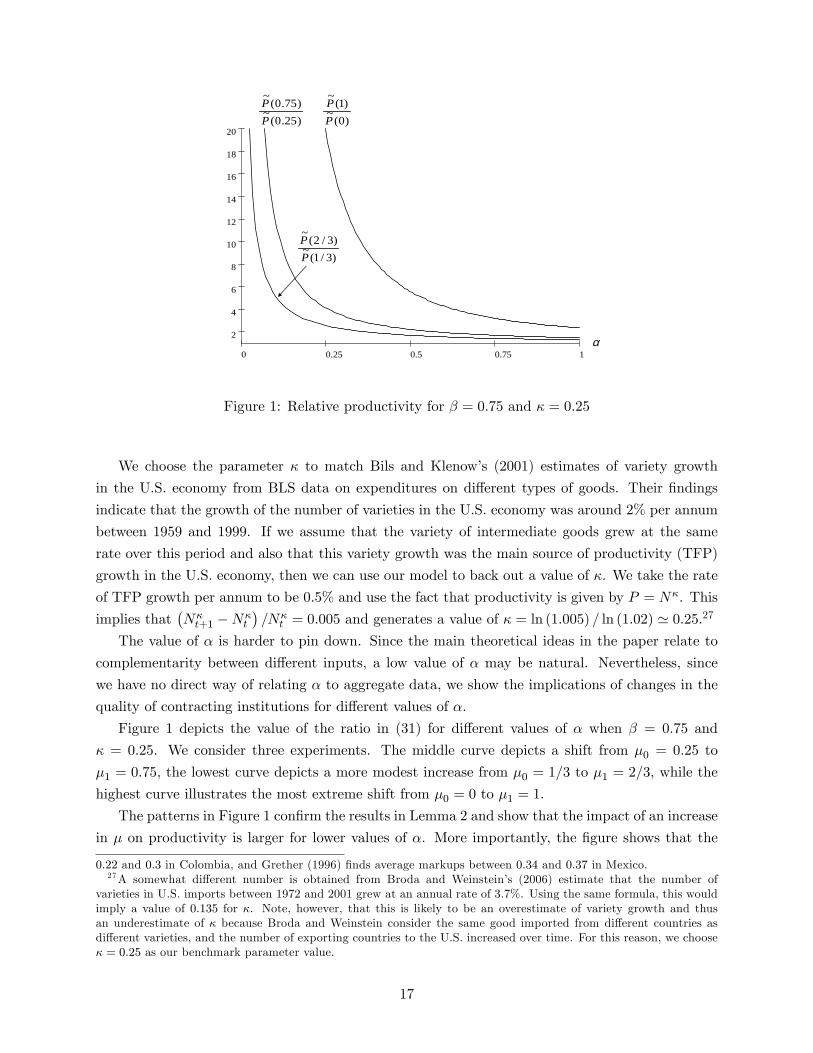
Figure 1: Relative productivity for � = 0:75 and � = 0:25

We choose the parameter � to match Bils and Klenow�s (2001) estimates of variety growth

in the U.S. economy from BLS data on expenditures on di¤erent types of goods. Their �ndings

indicate that the growth of the number of varieties in the U.S. economy was around 2% per annum

between 1959 and 1999. If we assume that the variety of intermediate goods grew at the same

rate over this period and also that this variety growth was the main source of productivity (TFP)

growth in the U.S. economy, then we can use our model to back out a value of �. We take the rate

of TFP growth per annum to be 0.5% and use the fact that productivity is given by P = N�. This

implies that�N�t+1 �N�

t

�=N�

t = 0:005 and generates a value of � = ln (1:005) = ln (1:02) ' 0:25.27

The value of � is harder to pin down. Since the main theoretical ideas in the paper relate to

complementarity between di¤erent inputs, a low value of � may be natural. Nevertheless, since

we have no direct way of relating � to aggregate data, we show the implications of changes in the

quality of contracting institutions for di¤erent values of �.

Figure 1 depicts the value of the ratio in (31) for di¤erent values of � when � = 0:75 and

� = 0:25. We consider three experiments. The middle curve depicts a shift from �0 = 0:25 to

�1 = 0:75, the lowest curve depicts a more modest increase from �0 = 1=3 to �1 = 2=3, while the

highest curve illustrates the most extreme shift from �0 = 0 to �1 = 1.

The patterns in Figure 1 con�rm the results in Lemma 2 and show that the impact of an increase

in � on productivity is larger for lower values of �. More importantly, the �gure shows that the

0:22 and 0:3 in Colombia, and Grether (1996) �nds average markups between 0:34 and 0:37 in Mexico.27A somewhat di¤erent number is obtained from Broda and Weinstein�s (2006) estimate that the number of

varieties in U.S. imports between 1972 and 2001 grew at an annual rate of 3.7%. Using the same formula, this wouldimply a value of 0:135 for �. Note, however, that this is likely to be an overestimate of variety growth and thusan underestimate of � because Broda and Weinstein consider the same good imported from di¤erent countries asdi¤erent varieties, and the number of exporting countries to the U.S. increased over time. For this reason, we choose� = 0:25 as our benchmark parameter value.

17

10.750.50.250

25

22.5

20

17.5

15

12.5

10

7.5

5

2.5

β=0.75 β=0.78

β=0.70

α

Figure 2: Relative productivity ~P (0:75) = ~P (0:25) for � = 0:25 and alternative ��s.

quantitative e¤ects can be sizable for a large range of values of �. For example, when � = 0:25,

productivity increases by a factor of 2:5, 4:1 and 19:7 in the three experiments. However, as �

increases and intermediate inputs become more substitutable, the magnitude of the quantitative

e¤ects diminishes. For example, when � = 0:75, productivity increases, respectively, by a factor of

1:4, 1:7, and 3:2 in the three cases. Though smaller, these are still sizable e¤ects.

We next discuss the sensitivity of these quantitative results to alternative parameter values.

While markup estimates are consistent with a value of � = 0:75, other evidence suggests somewhat

higher or lower values of �. Figure 2 shows the results of an increase in � from 0:25 to 0:75 when

� = 0:78 and when � = 0:7, while leaving � at 0:25.28 The �gure shows that the quantitative

e¤ects are considerably larger in the case in which � = 0:78, even for large values of �. For

example, with � = 0:75, the improvement in contracting institutions leads to a proportional increase

in productivity of 4:4, which is a very sizable e¤ect. Setting � equal to 0:7 reduces the e¤ect of

improved contractibility on productivity, but for � = 0:25 we still �nd that the experiment increases

productivity by a factor of 1:8.

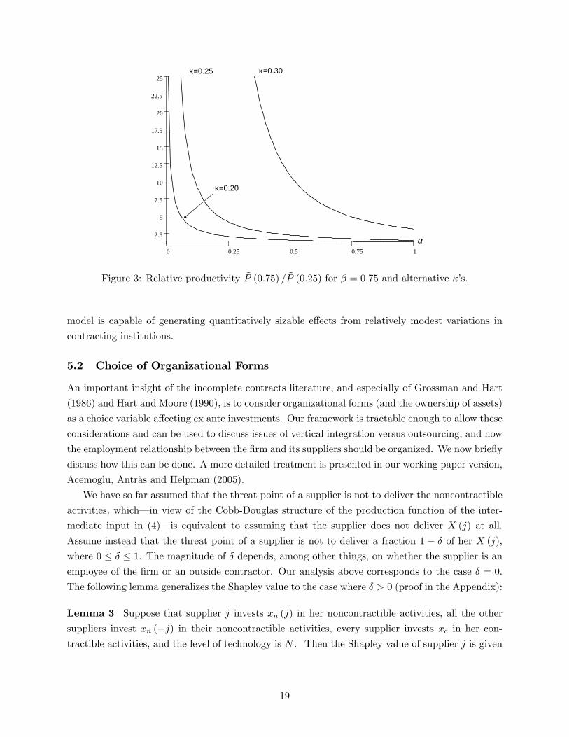
Finally, Figure 3 shows the results for alternative values of �, � = 0:2 and � = 0:3, while holding

� at 0:75. When � = 0:2; the estimated e¤ects are somewhat smaller than in our benchmark

simulation, but still sizable; with low values of �, the impact of an improvement in the quality

of contracting institutions on productivity is still large. For example, with � = 0:25, productivity

increases by a factor of 2:0. On the other hand, greater values of � lead to more signi�cant responses

of productivity to increases in �. Even for a very high value of � such as 0:75, productivity increases

by a factor of 4:8 as � increases from 0:25 to 0:75.

Overall, this simple quantitative evaluation suggests that the mechanism highlighted in our

28Only values of � less than 0:8 are consistent with Assumption 1 combined with � = 0:25:

18

10.750.50.250

25

22.5

20

17.5

15

12.5

10

7.5

5

2.5

κ=0.25 κ=0.30

κ=0.20

α

Figure 3: Relative productivity ~P (0:75) = ~P (0:25) for � = 0:75 and alternative ��s.

model is capable of generating quantitatively sizable e¤ects from relatively modest variations in

contracting institutions.

5.2 Choice of Organizational Forms

An important insight of the incomplete contracts literature, and especially of Grossman and Hart

(1986) and Hart and Moore (1990), is to consider organizational forms (and the ownership of assets)

as a choice variable a¤ecting ex ante investments. Our framework is tractable enough to allow these

considerations and can be used to discuss issues of vertical integration versus outsourcing, and how

the employment relationship between the �rm and its suppliers should be organized. We now brie�y

discuss how this can be done. A more detailed treatment is presented in our working paper version,

Acemoglu, Antràs and Helpman (2005).

We have so far assumed that the threat point of a supplier is not to deliver the noncontractible

activities, which� in view of the Cobb-Douglas structure of the production function of the inter-

mediate input in (4)� is equivalent to assuming that the supplier does not deliver X (j) at all.

Assume instead that the threat point of a supplier is not to deliver a fraction 1 � � of her X (j),where 0 � � � 1. The magnitude of � depends, among other things, on whether the supplier is anemployee of the �rm or an outside contractor. Our analysis above corresponds to the case � = 0.

The following lemma generalizes the Shapley value to the case where � > 0 (proof in the Appendix):

Lemma 3 Suppose that supplier j invests xn (j) in her noncontractible activities, all the other

suppliers invest xn (�j) in their noncontractible activities, every supplier invests xc in her con-tractible activities, and the level of technology is N . Then the Shapley value of supplier j is given

19

by (20), where

���1� ��+�

�(�+ �) (1� ��) : (32)

Lemma 3 implies that the formula for the Shapley value is the same as before, except that now

the �rm�s share in the bargaining game, , depends on �. Clearly, in (32) equals in (19) when

� = 0, but is greater when � > 0. This is natural, since, with � > 0, the bargaining game is more

advantageous to the �rm. In the limit as � goes to 1, the �rm�s share also goes to 1.

Using this lemma, the working paper version demonstrated that all the results in Propositions

2 and 3 hold for any � 2 [0; 1) and employed this generalization to analyze the choice betweenintegration and outsourcing. Brie�y, suppose that for an integrated �rm, we have � > 0, while with

outsourcing � = 0.29 Then, when the choice of the upfront payment � is not restricted, it can be

shown that the �rm always prefers outsourcing to vertical integration.30 In contrast, when suppliers

face credit constraints (in the sense that the upfront payment � is restricted to be nonnegative),

integration may be preferable to outsourcing. In particular, when credit constraints are present and

�+� < 1, there exists �� 2 (0; 1) such that vertical integration is preferred by the �rm for � < �� andoutsourcing is preferred for � > ��. Furthermore, �� is decreasing in �, so that integration is more

likely when there is greater complementarity between intermediate inputs. This result implies that

vertical integration is more likely when both contractual frictions and credit market imperfections

are present.31

5.3 General Equilibrium

We now discuss how the technology choice can be embedded in a general equilibrium version

of our model. Besides verifying that general equilibrium interactions do not reverse our partial

equilibrium results, this analysis is useful as a preparation for the results in the next subsection,

where we investigate endogenous patterns of comparative advantage across countries. We start

with an equilibrium with a given number of producers (�nal goods) and then endogenize this with

free entry. In this and the next subsection, we focus on the case where 0 < � < 1, and � = 0 as in

the baseline model.

Assume that there exists a continuum of �nal goods q (z), with z 2 [0; Q], where Q represents

the number (measure) of �nal goods. All consumers have identical preferences,

u =

�Z Q

0q (z)� dz

�1=�� cxe; 0 < � < 1; (33)

29An integrated �rm has � > 0 because in this case the �rm owns all the intermediate inputs. In this event themost a supplier can do is not to cooperate in the use of her intermediate input, which will reduce the e¢ ciency withwhich the �rm can employ this input, but may not reduce this e¢ ciency to zero. See Grossman and Hart (1986).30This is because the �rm does not undertake any relationship-speci�c investments. Since suppliers are the only

agents undertaking noncontractible relationship-speci�c investments, it is e¢ cient to give them as much bargainingpower as possible. This will not necessarily be the case if the �rm were to also make relationship-speci�c investments.See, for example, Hart and Moore (1990), Antràs (2003, 2005), and Antràs and Helpman (2004).31The positive e¤ect of complementarity on the integration decision has been derived before in the property-rights

literature (see Hart and Moore, 1990).

20

where e is the total e¤ort exerted by this individual and the elasticity of substitution between �nal

goods, 1= (1� �), is greater than 1, and cx represents the cost of e¤ort in terms of real consumption.These preferences imply the demand function

q (z) =

�p (z)

pI

��1=(1��) SpI;

where p (z) is the price of good z, S is the aggregate spending level, and

pI ��Z Q

0p (z)��=(1��) dz

��(1��)=�is the ideal price index, which we take to be the numeraire, i.e., pI = 1. The implied demand

function A [p (z)]�1=(1��) for each �rm is therefore identical to the demand function used in the

previous sections, with A = S.

Recall that each �rm in this economy solves the maximization problem (24) and its reduced-

form pro�t function is given by (29). We assume that the degree of technological complementarity,

�, varies across �rms (or sectors) with its support given by a subset of (0; 1). We denote its

cumulative distribution function byH (�). This formulation implies that if Q products are available

for consumption, a fractionH (�) of them are produced with elasticities of substitution smaller than

1= (1� �).The key general equilibrium interaction results from competition of producers for a scarce

resource, labor. Assume that labor is in �xed supply L. A �rm that adopts technologyN employsN

individuals as suppliers and CL (N) workers in the process of technology adoption (implementation,

use, or creation of the technology). We assume that these are the only uses of labor (Assumption 1

now applies to CL (N)). Denoting the wage rate in terms of the numeraire by w, this implies that

the total cost of adopting technology N is C (N) = wCL (N). The wage rate w is taken as given

by each �rm, but is endogenously determined in equilibrium.

The �rst-order condition of the maximization of (29) yields:

��

1� �AZ (�; �)N�(�+1)�1

1�� = wC 0L (N) + w0; for all � 2 (0; 1) . (34)

Since each individual can be employed at the wage w in the process of technology adoption, their

outside option as a supplier is w0 = w. Equation (34) then implies that the technology choice

depends on a � A=w, which is the inverse real cost of technology adoption (or the �equilibrium

market size�). Let the equilibrium technology choice ofN as a function of a, �, and � implied by (34)

be N (a; �; �). De�ning total labor demand by a �rm with technology N as CT (N) � CL (N)+N ,condition (34) implies that N (a; �; �) is implicitly de�ned by

��

1� �aZ (�; �)N (a; �; �)�(�+1)�1

1�� = C 0T [N (a; �; �)] ; for all � 2 (0; 1) : (35)

21

Since �rms with higher elasticities of substitution choose higher N (Proposition 2), this equation

implies that N (a; �; �) is increasing in �. The demand for labor by a �rm choosing technology

N (a; �; �) is CT [N (a; �; �)], thus labor market clearing can be expressed as:32

Q

Z 1

0CT [N (a; �; �)] dH (�) = L; (36)

where the left-hand side is total demand for labor and L is labor supply. Since N (a; �; �) is

increasing in a, this condition uniquely determines the equilibrium value of a, i.e., our measure of

the real demand level. The relationship between a and the model�s parameters, as embodied in

this equation, illustrates the key general equilibrium feedback in our model. Proposition 2 implies

that N (a; �; �) is increasing in �, so we may expect better contracting institutions to encourage

all �rms to adopt more advanced technologies. However, the resource constraint, (36), implies that

not all the N (a; �; �)�s can increase with Q constant. Consequently, the equilibrium value of a has

to adjust to clear the labor market when � rises.

To derive the implications of an increase in � on the cross-sectional distribution of technology

choices, recall that the number of products, Q, is given, and di¤erentiate the �rst-order condition

(35) to obtain

a+ �� (�; �) � = � [N (a; �; �)] N (a; �; �) ; (37)

where y, de�ned as dy=y, represents the proportional rate of change of variable y, �� (�; �) is the

elasticity of Z (�; �) with respect to �, and � (N) is the elasticity of the marginal cost curve C 0T (N)

minus [� (�+ 1)� 1] = (1� �), i.e.,

� (N) � C 00T (N)N

C 0T (N)� � (�+ 1)� 1

1� � :

Assumption 1 implies that � (N) > 0. Moreover, as proved in Lemma 2 �� (�; �) > 0 and �� (�; �)

is decreasing in �. Next di¤erentiating (36), we obtain a relationship between � and a:Z 1

0�L (�) N (a; �; �) dH (�) = 0, (38)

where �L (�) � C 0T [N (a; �; �)]N (a; �; �). Substituting (37) into (38) then yields

a = �R 10 �L (�) �� (�; �)� [N (a; �; �)]

�1 dH (�)R 10 �L (�)� [N (a; �; �)]

�1 dH (�)�:

Since the term in front of � on the right-hand side of this equation is negative, an improvement in

contracting institutions increases wages relative to expenditure and reduces a.

Equation (38) shows that the proportional change in N in response to �, N (a; �; �), can be

positive only for some ��s (again because of the resource constraint). Since @�� (�; �) =@� < 0

32Since it is straightforward to verify that the wage is always strictly positive, (36) is written as an equality ratherthan in complementary slackness form.

22

(from Lemma 2), the left-hand side of equation (37) is decreasing in �. Consequently, there exists

a critical value �� such that N (a; �; �) > 0 for all � < �� and N (a; �; �) < 0 for all � > ��.

This implies that low � �rms, with greater technological complementarity between inputs, are more

contract dependent. This establishes the following proposition (proof in the text):

Proposition 4 Suppose Assumption 1 holds. Then there exists �� 2 (0; 1) such that in the generalequilibrium economy with Q constant, an increase in � raises the level of technology N (a; �; �) in

all �rms with � < �� and reduces it in all �rms with � > ��.

We next discuss how the number of products, Q, can be endogenized with free entry. To do

this in the simplest possible way, suppose that an entrant faces a �xed cost of entry wf , where f

is the amount of labor required for entry. This cost is borne in addition to the cost of technology

adoption. Moreover, in the spirit of Hopenhayn (1992) and Melitz (2003), suppose that an entrant

does not know a key parameter of the technology prior to entry. While in their models the entrant

does not know its own productivity, we assume instead that it does not know �, but knows that

� is drawn from the cumulative distribution function H (�). Since the relationship between � and

productivity is determined in general equilibrium, the distribution of productivity is endogenous.

After entry, each �rm learns its � and maximizes the pro�t function (29). This maximization

leads to the choice of technology as a function of a, �, and �, i.e., N (a; �; �), in (35). Let us de�ne

�(a; �; �) � aZ (�; �)N (a; �; �)1+�(�+1)�1

1�� � CT [N (a; �; �)] ;

where Z (�; �) is given by (30). This is an indirect pro�t function, with pro�ts measured in units

of labor. It is straightforward to verify that it is increasing in a, � and �.

Free entry implies that expected pro�ts must equal the entry cost wf , orZ 1

0�(a; �; �) dH (�) = f: (39)

This free entry condition uniquely determines the equilibrium value of a, without reference to

the labor market clearing condition (36). Consequently, given the equilibrium value of a, the

distribution of � induces a distribution of productivity and �rm size in the economy (from the

�rst-order condition (35)): �rms with larger ��s choose more advanced technologies and they are

more productive.33

Finally, the labor market clearing condition determines the number of entrants. Since labor

demand now includes individuals working in the founding of the �rms, the market clearing condition

33Note also that the degree of dispersion of productivity depends on the degree of contract incompleteness; incountries with better contracting institutions there is less productivity dispersion and less size dispersion. Thisfollows from the fact that small �rms (i.e., low-� �rms) are larger in countries with better contracting institutions,while large �rms (high-� �rms) are smaller in those same countries. This prediction of the model is consistent withthe empirical evidence reported in Tybout (2000), which indicates that there are signi�cantly fewer medium-sizedenterprises in less-developed economies, which typically have worse contracting institutions.

23

(36) has to be replaced with

Q

�Z 1

0CT [N (a; �; �)] dH (�) + f

�= L:

Together with N (a; �; �) from (35) and a from the free entry condition (39), this modi�ed labor

market clearing condition determinants the number of entrants Q.

An interesting implication of the general equilibrium with free entry is that an increase in the

supply of labor L does not create a scale e¤ect and is not a source of comparative advantage. If

two countries that di¤er only in L freely trade with each other, their wages are equalized, their

technology level is the same in every industry �, and they have the same distribution of productivity

and �rm size. The only di¤erence is that the larger country has proportionately more �nal good

producers. This result contrasts with the case with an exogenous number of products, where

di¤erences in L would generate comparative advantage.34

5.4 Comparative Advantage

Perhaps the most interesting general equilibrium application of our framework is to international

trade. Consider a world consisting of two countries, indexed by ` = 1; 2. We now derive an

endogenous pattern of comparative advantage between these two countries from di¤erences in

contracting institutions.35 Suppose that there is a �xed number of products and that every product

is distinct not only from other products produced in its own country, but also from products

produced in the foreign country. All products can be freely traded between the two countries.

Suppose also that the two countries are identical, except for their contracting institutions. In

particular, L1 = L2, Q1 = Q2 and H1 (�) = H2 (�) for all � 2 (0; 1), but the fraction of activities�` that are contractible di¤ers across countries. Without loss of generality, we assume that �1 > �2,

so that country 1 has better contracting institutions.

The equilibrium condition for technology adoption (34) holds in both countries, with di¤er-

ent wage rates, w`, for the two countries (A is the same for both countries and equal to world

expenditure). De�ning a` � A=w` and N ` (�) � N�a`; �; �`

�, we have

��

1� �a`Z��; �`

�N ` (�)

�(�+1)�11�� = C 0T

hN ` (�)

i; for all � 2 (0; 1) ; ` = 1; 2: (40)

In addition, the labor market clearing condition (36) holds in both countries. Consequently, the

country with better contracting institutions, country 1, will have higher wages and a lower a`.36

The pattern of trade can now be determined by comparing the revenues of �rms with the same

value of � in the two countries. We show in the Appendix (see the proof of Proposition 2) that the

34We have also worked out an endogenous growth model with expanding product variety, where the long-run rateof growth depends on the degree of contract incompleteness. We do not discuss this model in order to save space.35The link between contracting institutions and endogenous comparative advantage was previously discussed by

Levchenko (2003), Costinot (2004), Nunn (2005) and Antràs (2005).36Suppose not, then (40) implies N1 (�) > N2 (�) for all ��s (since N ` (�) is increasing in � for given a), and so

labor market clearing cannot be satis�ed in both countries.

24

revenue of a producer with parameter � in country ` is

R` (�) = AZ��; �`

�N ` (�)

��1��

1� ��1� �`

�(1� �)

h1� � (1� �`) �

�+�

i ; (41)

which is increasing in total world expenditure, A, in Z (�; �) ; and in the level of technology. But

it is also directly a¤ected by the parameters through the last term on the right-hand side.

If R1 (�) =R2 (�) >R 10 R

1 (�) dH (�) =R 10 R

2 (�) dH (�), then country 1 is a net exporter of

goods with substitution parameter �. Consequently, we simply need to determine the distribution

of R1 (�) =R2 (�) across di¤erent ��s. >From (41) we have

R1 (�)

R2 (�)=Z��; �1

�Z (�; �2)

�N1 (�)

N2 (�)

� ��1�� 1� �

�1� �1

�1� � (1� �2)

1� ��1� �2

���+�

1� � (1� �1) ��+�

: (42)

Both Z��; �1

�=Z��; �2

�and the last term in (42) are decreasing in �.37 Second, Proposition 4

implies that there exists an �� such that N1 (�) < N2 (�) for all � > �� and N1 (�) > N2 (�) for all

� < ��. As a result, country 1, which has the better contracting institutions, tends to export low-�

products and import high-� products. If, in addition, � (N) is constant, the proportional change in

N (a; �; �) in response to an increase in � is always smaller when � is greater (because the partial

@�� (�; �) =@� is negative, see Lemma 2). In this case, R1 (�) =R2 (�) is everywhere decreasing in �

and there exists ��� 2 (0; 1) such that R1 (�) =R2 (�) >R 10 R

1 (�) dH (�) =R 10 R

2 (�) dH (�) for all

� < ��� and the opposite inequality holds for all � > ���. Consequently, country 1, with the better

contracting institutions, is a net exporter in low-� sectors and a net importer in high-� sectors.

This result is summarized in the following (proof in the text):

Proposition 5 Suppose Assumption 1 holds and � (N) is constant. Then there exists ��� 2 (0; 1)such that in the two-country world equilibrium country 1 with �1 > �2 is a net exporter of products

with � < ��� and a net importer of products with � > ���.

The most important implication of this result is that di¤erences in contracting institutions create

endogenous comparative advantage. A country with better contracting institutions gains a com-

parative advantage in sectors that are more contract dependent, which, in our model, correspond

to the sectors with greater technological complementarities between inputs.

The main implications in Proposition 5 receive support from a number of recent empirical

papers. Nunn (2005) and Levchenko (2003) use international trade data and the classi�cation of

industries into more and less �contract dependent� groups. Consistent with Proposition 5, they

�nd that countries with better contracting institutions specialize in the export of goods that are

more �contract dependent�. Moreover, the impact of cross-country di¤erences in the contracting

institutions on exports is quantitative large. Nunn, for example, �nds that the estimated impact

37Recall from Lemma 2 that Z (�; �) is increasing in � and �, and @�� (�; �) =@� < 0. Therefore Z��; �1

�=Z��; �2

�is decreasing in � whenever �1 > �2. The fact that the last term is decreasing in � follows from �1 > �2.

25

of the quality of the legal system on the export of contract-dependent sectors is comparable to the

e¤ect of human capital abundance on the export of human capital intensive products. In other

words, according to these estimates, di¤erences in legal systems are as important as di¤erences in

human capital abundance for explaining trade �ows.

6 Conclusion

In this paper, we developed a tractable framework for the analysis of the impact of contractual

incompleteness and technological complementarities on the equilibrium technology choice. In our

model, a �rm chooses its technology corresponding to the range of intermediate inputs used in

production, and o¤ers contracts to suppliers, specifying the required investments in contractible

activities. Investments in the remaining, noncontractible activities are then chosen by the suppliers

in anticipation of the ex post bargaining payo¤s.

We used the Shapley value to characterize the division of surplus between the �rm and its

suppliers, and derived an explicit solution to these payo¤s. Using this setup, we established that

greater contractual incompleteness reduces investments in noncontractible and contractible activ-

ities and depresses technology choice. The impact of contractual incompleteness on technology

adoption is greater in sectors with more complementary intermediate inputs.

The key mechanism developed in the paper leads to potentially large di¤erences in productivity

in response to di¤erences in contracting institutions. We also derived implications of this mechanism

for di¤erences in the internal organization of the �rm across societies with di¤erent contracting

institutions and a new mechanism for endogenous comparative advantage. These implications are

consistent with a range of recent empirical results in the literature.

It is also useful to note that while we have used a �love-for-variety�model of technology, our

results do not depend on this speci�c modeling approach. In equation (29) N can be interpreted

as a general technological investment, and the linkages between contracts and technology adoption

(or investment) highlighted in our analysis would apply independent from the speci�c assumptions

regarding the nature of technology.

A number of areas are left for future research. These include, but are not limited to, the

following. The model assumes that all activities are symmetric; an important extension is to see

whether similar results hold with a more general production function, where the �rm may wish

to treat some suppliers of intermediate inputs di¤erently than others, depending, for example, on

how essential they are for production. Another area for future study is an investigation of the

simultaneous determination of the range of intermediate inputs used by the �rm and the division

of labor among the suppliers. Finally, it is important to investigate whether the relationship

between contracting institutions, technological complementarities, and the choice of technology, is

fundamentally di¤erent when we use alternative approaches to the theory of the �rm, such as the

managerial incentives approach of Holmström and Milgrom (1991).

26

Appendix

Second-Order Conditions in the Complete Contracting Case

Let � = A1��N�(�+1)x� � cxNx�C (N)�w0N . Using the �rst-order conditions (11) and (12), the matrixof the second-order conditions can be expressed as:

@2�=@x2 @2�=@x@N

@2�=@N@x @2�=@N2

!=

� (1� �)�Nc2x (C 0 + w0)

�1 �cx [1� � (1 + �)]�cx [1� � (1 + �)] �N�1 [1� � (1 + �)] (�+ 1)��1 (C 0 + w0)� C 00

!:

The second-order conditions are satis�ed if this matrix is negative de�nite, which requires its diagonal

elements to be negative and its determinant to be positive. The �rst diagonal element is negative; the

second diagonal element is negative if and only if

C 00N

C 0 + w0>[� (1 + �)� 1] (�+ 1)

�;

and the determinant is positive if and only if

C 00N

C 0 + w0>� (1 + �)� 1

1� � :

Note that if � (1 + �) < 1 both of these conditions are satis�ed, and if � (1 + �) � 1, the second inequalityimplies the �rst inequality. Therefore Assumption 1 is necessary and su¢ cient for the second-order conditions

to be satis�ed.

Proof of Proposition 1

The �rst part of the proposition is a direct implication of Assumption 1. The comparative statics of N� follow

from the implicit function theorem by noting that, except for �, N� increases in response to an increase in

a parameter if and only if this parameter raises the left-hand side of (11). Using the results concerning the

response of N� to changes in parameters together with (12) then implies the responses of x� to parameter

changes.

Proof of Lemma 1 and Related Results

We develop here a more formal proof than the one in the main text that builds on the work of Aumann

and Shapley (1974). Let there be M suppliers each one controlling a range " = N=M of the continuum

of intermediate inputs. Due to symmetry, all suppliers provide an amount xc of contractible activities. As

for the noncontractible activities, consider a situation in which a supplier j supplies an amount xn (j) per

noncontractible activity, while the M � 1 remaining suppliers supply the same amount xn (�j) (note thatwe are again appealing to symmetry).

To compute the Shapley value for this particular supplier j, we need to determine the marginal contri-

bution of this supplier to a given coalition of agents. A coalition of n suppliers and the �rm yields a sales

revenue of

FIN (n;N ; ") = A1��N�(�+1�1=�)x��c

h(n� 1) "xn (�j)(1��)� + "xn (j)(1��)�

i�=�, (A1)

27

when the supplier j is in the coalition, and a sales revenue

FOUT (n;N ; ") = A1��N�(�+1�1=�)x��c

hn"xn (�j)(1��)�

i�=�(A2)

when supplier j is not in the coalition. Notice that even when n < N , the term N�(�+1�1=�) remains in

front, because it represents a feature of the technology, though productivity su¤ers because the term in

square brackets is lower.

Following the notation in the main text, the Shapley value of player j is

sj =1

(M + 1)!

Xg2G

�v�zjg [ j

�� v

�zjg��: (A3)

The fraction of permutations in which g (j) = i is 1= (M + 1) for every i. If g (j) = 0 then v�zjg [ j

�=

v�zjg�= 0, because in this event the �rm is necessarily ordered after j. If g (j) = 1 then the �rm

is ordered before j with probability 1=M and after j with probability 1 � 1=M . In the former case

v�zjg [ j

�= FIN (1; N ; "), while in the latter case v

�zjg [ j

�= 0. Therefore the conditional expected

value of v�zjg [ j

�, given g (j) = 1, is 1

M FIN (1; N ; "). By similar reasoning, the conditional expected

value of v�zjg�is 1

M FOUT (0; N ; "). Repeating the same argument for g (j) = i, i > 1, the conditional ex-

pected value of v�zjg [ j

�, given g (j) = i, is i

M FIN (i;N ; "), and the conditional expected value of v�zjg�is

iM FOUT (i� 1; N ; "). It follows from (A3) that

sj =1

(M + 1)M

MXi=1

i [FIN (i;N ; ")� FOUT (i� 1; N ; ")]

=1

(N + ")N

MXi=1

i" [FIN (i;N ; ")� FOUT (i� 1; N ; ")] ":

Substituting for (A1) and (A2),

sj =A1��N�(�+1�1=�)x��c

(N + ")N

MXi=1

i"ni"xn (�j)(1��)� + "

hxn (j)

(1��)� � xn (�j)(1��)�io�=�

"

�A1��N�(�+1�1=�)x��c

(N + ")N

MXi=1

i"hi"xn (�j)(1��)� � "xn (�j)(1��)�

i�=�".

For " small enough, the �rst-order Taylor expansion gives

sj 'A1��N�(�+1�1=�)x��c (�=�) "xn (j)

(1��)�

(N + ")N

MXi=1

(i")hi"xn (�j)(1��)�

i(���)=�";

or

sj"'A1��N�(�+1�1=�) (�=�)

hxn(j)xn(�j)

i(1��)�x��c xn (�j)

�(1��)

(N + ")N

MXi=1

(i")�=�

":

Now taking the limit as M ! 1, and therefore " = N=M ! 0, the sum on the right-hand side of this

28

equation becomes a Riemann integral:

limM!1

�sj"

�=A1��N�(�+1�1=�) (�=�)

hxn(j)xn(�j)

i(1��)�x��c xn (�j)

�(1��)

N2

Z N

0

z�=�dz:

Solving the integral delivers

limM!1

(sj=") = (1� )A1���xn (j)

xn (�j)

�(1��)�x��c xn (�j)

�(1��)N�(�+1)�1,

with = �= (�+ �). This corresponds to equation (20) in the main text, and completes the proof of the

lemma.

In addition, imposing symmetry, i.e., xn (j) = xn (�j), the �rm�s payo¤ is

s0 = A1��N�(�+1)x��c xn

�(1��) �Nsj = A1��x��c x�(1��)n N�(�+1),

as stated in equation (22) in the text.

Proof of Proposition 2

First, we verify that the second-order conditions are again satis�ed under Assumption 1. To see this, note

that the problem in (14) is strictly concave and delivers a unique xn = �xn (N;xc), as given in (23). Plugging

this expression into (24) we obtain

� = A1��

1��(1��)N1+�(�+1)�11��(1��)x��=[1��(1��)]c � cxxcN�� C (N)� w0N (A4)

where

�h(cx)

�1� (1� )

i�(1��)=[1��(1��)][1� � (1� �) (1� )] .

The second-order conditions can be checked, analogously to the case with complete contracts, by computing

the Hessian and checking that it is negative de�nite.

Here, we present an alternative proof which also serves to illustrate how the reduced-form pro�t function

(29) in the main text is derived. In particular, notice that for a given level of N , the problem of choosing xcis convex (since �� < 1� � + ��) and delivers a unique solution:

xc = A

��c�1x

1� � (1� �)

�[1��(1��)]=(1��)N

�(�+1)�11�� . (A5)

Plugging this solution in (A4) then delivers

� = AZN1+�(�+1)�1

1�� � C (N)� w0N;

where

Z ��

�c�1x1� � (1� �)

���=(1��)[1��(1��)]=(1��)

�1� �

1� � (1� �)

�,

which simpli�es to equation (30) in the text. This reduced-form expression of the pro�t function immediately

implies that @2�=@N2 < 0 if and only if the second part of Assumption 1 holds. Finally, from equation

(A5) we also have cxxcN� = AZN1+

�(�+1)�11�� ��= (1� �), which combined with (19) and (28) implies that

29

the �rm�s revenues are

R = � + C (N) + w0N + cxxcN�+ cxxnN (1� �)

= AZN1+�(�+1)�1

1��

0@ 1� � (1� �)(1� �)

h1� � (1� �) �

�+�

i1A ,

which will be used in Section 5.3 (see equation (41)).

Next, the comparative static results follow from the implicit function theorem as in the proof of Propo-

sition 1. First, @ ~N=@A > 0 follows immediately. To show that @ ~N=@� > 0 and @ ~N=@� > 0, let us take

logarithms of both sides of (25), to obtain

� (�+ 1)� 11� � ln ~N + ln

�A��

11�� c

� �1��

x

�+ F (#; �) = ln

�C 0�~N�+ w0

�;

where

F (#; �) =1� � (1� �)

1� � ln

�1� # (1� �)1� � (1� �)

�+� (1� �)1� � ln

�#��1

�, (A6)

and # � � (1� ) < � is monotonically increasing in �. Simple di¤erentiation delivers

@F (#; �)

@#=

(1� �) (� � #)(1� �)# (1� # (1� �)) ,

which implies @F=@� > 0, and establishes that @ ~N=@� > 0.

Furthermore,

@F (#; �)

@�=#� � + � (1� # (1� �))

�ln�1�#(1��)1��(1��)

�+ ln

��#

��(1� # (1� �)) (1� �)

and@2F (#; �)

@�2= � (� � #)2

(1� # (1� �))2 (1� � (1� �)) (1� �)< 0.

Thus, @F (#; �) =@� reaches its minimum over the set � 2 [0; 1] at � = 1, in which case it equals

#� � + � ln (�=#)1� � > 0:

This inequality follows from the fact that #� � + � ln (�=#) is decreasing in # for # < �, and is equal to 0at # = �. We thus have shown that @F (#; �) =@� > 0 for all �, so that @ ~N=@� > 0.

Finally, note that straightforward di¤erentiation of (28) delivers @ (~xn=~xc) =@A = 0, @ (~xn=~xc) =@� > 0

and @ (~xn=~xc) =@� > 0. And, in light of equation (26), the e¤ects of A, � and � on ~xc follow directly from

those on ~N , where the inequalities become strict whenever C 00 (�) > 0.

Proof of Lemma 2

Comparison of (30) with (A6) implies that

Z (�; �) � 'eF (#;�);

30

where

# � � (1� ) = ��

�+ �

and ' is a parameter that only depends on � and cx. We have that F (#; �) is increasing in both its

arguments, and that # is increasing in �, which establish part 1 of the lemma. To prove part 2, �rst note

that@2F (#; �)

@#@�=

� (� � #)(1� # (1� �))2 # (1� �)

< 0,

because # < �. Moreover,

�� (�; �) ��

Z

@Z (�; �)

@�= �

@F (#; �)

@�;

and therefore@�� (�; �)

@�= �

@2F (#; �)

@#@�� @#

@�< 0.

Similarly,

�� (�; �) ��

Z

@Z (�; �)

@�= �

@F (#; �)

@#� @#

@�;

and therefore@�� (�; �)

@�= �

@2F (#; �)

@#@�� @#

@�< 0.

Proof of Proposition 3

The proof follows from Proposition 2, sincen~N; ~xc

oconverge to fN�; x�g as �! 1, and ~N; ~xc; and ~xn are

all increasing in � (nondecreasing in �, in the case of the investment levels).

Proof of Lemma 3

The proof is similar to that of Lemma 1. A coalition of n suppliers and the �rm yields a sales revenue of

FIN (n;N ; ") = A1��N�(�+1�1=�)x��c

h(n� 1) "xn (�j)(1��)� + "xn (j)(1��)� + (N � n") ��xn (�j)(1��)�

i�=�,

(A7)

when the supplier j is in the coalition, and a sales revenue

FOUT (n;N ; ") = A1��N�(�+1�1=�)x��c

hn"xn (�j)(1��)� + "��xn (j)(1��)� + (N � (n+ 1) ") ��xn (�j)(1��)�

i�=�(A8)

when supplier j is not in the coalition.

As in the case with � = 0, the Shapley value of supplier j can be written as

sj =1

(N + ")N

MXi=1

i" [FIN (i;N ; ")� FOUT (i� 1; N ; ")] ":

Plugging the new formulas for FIN (n;N ; ") and FOUT (n;N ; ") in (A7) and (A8) then delivers

31

sj =A1��N�(�+1�1=�)x��c

(N + ")N

MXi=1

i"

(i" (1� ��)xn (�j)(1��)� + "

hxn (j)

(1��)� � xn (�j)(1��)�i

+N��xn (�j)(1��)�

)�=�"

�A1��N�(�+1�1=�)x��c

(N + ")N

MXi=1

i"

"i" (1� ��)xn (�j)(1��)� + "

h��xn (j)

(1��)� � xn (�j)(1��)�i

+N��xn (�j)(1��)�

#�=�":

For " small enough, the �rst-order Taylor expansion gives

sj"'A1��N�(�+1�1=�) (�=�) (1� ��)

hxn(j)xn(�j)

i(1��)�x��c xn (�j)

�(1��)

(N + ")N

MXi=1

(i") [(i") (1� ��) +N��](���)=� ":

Taking the limit as M !1, now yields

limM!1

�sj"

�=A1��N�(�+1�1=�) (�=�) (1� ��)

hxn(j)xn(�j)

i(1��)�x��c xn (�j)

�(1��)

N2

Z N

0

z [z (1� ��) +N��](���)=� dz:

Finally, integrating by parts delivers

limM!1

(sj=") = (1� )A1���xn (j)

xn (�j)

�(1��)�x��c xn (�j)

�(1��)N�(�+1)�1,

where

���1� ��+�

�(�+ �) (1� ��) ,

as claimed in the Lemma.

32

References

Acemoglu, Daron, Pol Antràs, and Elhanan Helpman (2005), �Contracts and the Division of

Labor,�NBER Working Paper No. 11356.

Acemoglu, Daron and Fabrizio Zilibotti (1999), �Information Accumulation in Development,�

Journal of Economic Growth, 4, pp. 5-38.

Amaral, Pedro S. and Erwan Quintin (2005), �Finance Matters,�mimeo.

Antràs, Pol (2003), �Firms, Contracts, and Trade Structure,�Quarterly Journal of Economics,

118:4, pp. 1375-1418.

Antràs, Pol (2005), �Incomplete Contracts and the Product Cycle,�American Economic Review,

95:4, pp. 1054-1073.

Antràs, Pol and Elhanan Helpman (2004), �Global Sourcing,�Journal of Political Economy 112:3,

pp. 552-580.

Aumann, Robert J. and Lloyd S. Shapley (1974), Values of Non-Atomic Games, Princeton Uni-

versity Press, Princeton, NJ.

Barro, Robert J., and Xavier Sala-i-Martin (2003), Economic Growth, Second Edition, Cambridge:

MIT Press.

Bakos, Yannis and Erik Brynjolfsson (1993), �From Vendors to Partners: Information Technol-

ogy and Incomplete Contracts in Buyer-supplier Relationships,� Journal of Organizational

Computing 3:3, pp. 301-328.

Basu, Susanto (1995), �Intermediate Goods and Business Cycles: Implications for Productivity

and Welfare,�American Economic Review 85:3, pp. 512-531.

Becker, Gary S. and Kevin M. Murphy (1992), �The Division of Labor, Coordination Costs, and

Knowledge,�Quarterly Journal of Economics, 107:4, pp. 1137-1160.

Benassy, Jean-Pascal (1998), �Is there always too little research in endogenous growth with ex-

panding product variety?,�European Economic Review, 42:1, pp. 61-69.

Bils, Mark and Peter J. Klenow (2001), �The Acceleration in Variety Growth,�American Eco-

nomic Review (Papers and Proceedings), 91:2, pp. 274-280.

Blanchard, Olivier and Michael Kremer (1997), �Disorganization,� Quarterly Journal of Eco-

nomics, Vol. 112:4, pp. 1091-1126.

Broda, Christian and David E. Weinstein (1996), �Globalization and the Gains from Variety,�

Quarterly Journal of Economics CXXI:2, pp.541-585.

33

Caselli, Francesco (2004), �Accounting for Cross-Country Income Di¤erences,�forthcoming in the

Handbook of Economic Growth.

Castro, Rui, Gian Luca Clementi and Glenn MacDonald (2004), �Investor Protection, Optimal

Incentives, and Economic Growth,�Quarterly Journal of Economics CXIX:3, pp. 1131-1175.

Costinot, Arnaud (2004), �Contract Enforcement, Division of Labor and the Pattern of Trade,�

manuscript Princeton University.

Erosa, Andrés and Ana Hidalgo Cabrillana (2005), �On Capital Market Imperfections as a Source

of Low TFP and Economic Rents,�mimeo.

Ethier, Wilfred J (1982), �National and International Returns to Scale in the Modern Theory of

International Trade,�American Economic Review, 72:3, pp. 389-405.

de Fontenay, Catherine C. and Joshua S. Gans (2003), �Organizational Design and Technology

Choice under Intra�rm Bargaining: Comment,�American Economic Review, 93:1, pp. 448-

455.

Francois, Patrick and Joanne Roberts (2003), �Contracting Productivity Growth,� Review of

Economic Studies, 70, pp. 59-85.

Grether, Jean-Marie (1996), �Mexico, 1985-90: Trade Liberalization, Market Structure, and Man-

ufacturing Performance,�in Mark J. Roberts and James R. Tybout (eds.) (1996) Industrial

Evolution in Developing Countries: Micro Patterns of Turnover, Productivity, and Market

Structure, New York, Oxford University Press.

Griliches, Zvi (1998) R&D and Productivity: the Econometric Evidence, University Of Chicago

Press, Chicago.

Grossman, Sanford J., and Oliver D. Hart (1986), �The Costs and Bene�ts of Ownership: A

Theory of Vertical and Lateral Integration,�Journal of Political Economy, 94:4, pp. 691-719.

Grossman, Gene and Elhanan Helpman (1991), Innovation and Growth in the Global Economy,

Cambridge, MA, MIT Press.

Hall, Robert and Charles I. Jones (1999), �Why Do Some Countries Produce So Much More

Output per Worker Than Others?,�Quarterly Journal of Economics, 114:1, pp. 83-116.

Hart, Oliver and John Moore (1990), �Property Rights and the Nature of the Firm,�Journal of

Political Economy, 98:6, pp. 1119-1158.

Holmström, Bengt (1982), �Moral Hazard in Teams,�Bell Journal of Economics, 13, pp. 324-40.

Holmström, Bengt and Paul Milgrom (1991), �Multiactivity Principal-Agent Analyses: Incentive

Contracts, Asset Ownership, and Job Design�Journal of Law, Economics and Organization

7, n0 (Special Issue): 24-52.

34

Hopenhayn, Hugo A. (1992), �Entry, Exit, and �rm Dynamics in Long Run Equilibrium,�Econo-

metrica, 60:5, pp. 1127-1150.

Klein, Benjamin, Crawford, Robert G., and Armen A. Alchian (1978), �Vertical Integration, Ap-

propriable Rents, and the Competitive Contracting Process,�Journal of Law and Economics,

21:2, pp. 297-326.

Klenow, Peter J. and Andres Rodriquez-Clare (1997), �The Neoclassical revival in Growth Eco-

nomics: Has It Gone Too Far?,�NBER Macroeconomics Annual, pp. 73-103.

Klette Tor Jacob (1996), �R&D, Scope Economies, and Plant Performance,� Rand Journal of

Economics, 27, pp. 502-22.

Klette Tor Jacob and Samuel Kortum (2004), �Innovating Firms and Aggregate Innovation,�

Journal of Political Economy, 112, pp. 986-1018.

Levchenko, Andrei (2003), �Institutional Quality and International Trade,�MIT Ph.D. disserta-

tion.

Maskin, Eric and Jean Tirole (1999) �Unforeseen Contingencies and Incomplete Contracts,�Re-

view of Economic Studies, 66, pp. 83-114.

Martimort David and Thierry Verdier (2000), �The Internal Organization of the Firm, Transaction

Costs and Macroeconomic Growth,�Journal of Economic Growth, 5, pp. 315-40.

Martimort David and Thierry Verdier (2004), �The Agency Cost of Internal Collusion and Schum-

peterian Growth,�Review of Economic Studies, 71, pp. 1119-41.

Melitz, Marc J. (2003), �The Impact of Trade on Intra-Industry Reallocations and Aggregate

Industry Productivity,�Econometrica, 71:6, pp. 1695-1725.

Morrison, Catherine J. (1992), �Unraveling the Productivity Growth Slowdown in the United

States, Canada and Japan: The E¤ects of Subequilibrium, Scale Economies and Markups,�

Review of Economics and Statistics LXXIV:3, pp. 381-393.

Nunn, Nathan (2005) �Relationship Speci�city, Incomplete Contracts and the Pattern of Trade,�

Quarterly Journal of Economics (forthcoming).

Osborne, Martin and Ariel Rubinstein (1994), A Course in Game Theory, MIT Press, Cambridge,

MA.

Quintin, Erwan (2003), �Limited Enforcement and the Organization of Production,�mimeo.

Roberts, Mark J. (1996), �Colombia, 1977-85: Producer Turnover, Margins, and Trade Exposure,�

in Mark J. Roberts and James R. Tybout (eds.) (1996) Industrial Evolution in Developing

Countries: Micro Patterns of Turnover, Productivity, and Market Structure, New York, Ox-

ford University Press.

35

Romer, Paul M. (1990), �Endogenous Technological Change,�Journal of Political Economy, IIC,

S71-S102.

Rotemberg, Julio J. and Michael Woodford (1991), �Markups and the Business Cycle,�in Olivier

Jean Blanchard and Stanley Fischer (eds.), NBER Macroeconomics Annual 1991, Cambridge,

MA, The MIT Press.

Shapley, Lloyd S. (1953), �A Value for N-Person Games,�in Contributions to the Theory of Games,

pp. 31�40, Princeton University Press, Princeton, NJ.

Stole, Lars A. and Je¤rey Zwiebel (1996a), �Organizational Design and Technology Choice under

Intra�rm Bargaining,�American Economic Review, 86:1, pp. 195-222.

Stole, Lars A. and Je¤rey Zwiebel (1996b), �Intra-Firm Bargaining under Non-Binding Con-

tracts,�Review of Economic Studies, 63:3, pp. 375-410.

Sutton, John (1988), Technology and Market Structure: Theory and History, MIT Press, Massa-

chusetts.

Tybout, James R. (2000), �Manufacturing Firms in Developing Countries: How Well Do They

Do, and Why?,�Journal of Economic Literature, 38:1, pp. 11-44

Williamson, Oliver E. (1975), Markets, Hierarchies: Analysis, Antitrust Implications, Free Press:

New York.

Williamson, Oliver E. (1985), The Economic Institutions of Capitalism, Free Press: New York.

Yang, Xiaokai and Je¤ Borland (1991), �A Microeconomic Mechanism for Economic Growth,�

Journal of Political Economy, 99:3, pp. 460-482.

36