Continuum mechanics of two-phase porous media - · PDF fileContinuum mechanics of two-phase...

Continuum mechanics of two-phase porous media

Ragnar Larsson

Division of material and computational mechanics

Department of applied mechanics

Chalmers University of TechnologyS-412 96 Göteborg, Sweden

Draft date December 15, 2012

Contents

Contents i

Preface 1

1 Introduction 3

1.1 Background . . . . . . . . . . . . . . . . . . . . . . . . . . . . . . . . . . . 3

1.2 Organization of lectures . . . . . . . . . . . . . . . . . . . . . . . . . . . . 6

1.3 Course work . . . . . . . . . . . . . . . . . . . . . . . . . . . . . . . . . . . 7

2 The concept of a two-phase mixture 9

2.1 Volume fractions . . . . . . . . . . . . . . . . . . . . . . . . . . . . . . . . 10

2.2 Effective mass . . . . . . . . . . . . . . . . . . . . . . . . . . . . . . . . . . 11

2.3 Effective velocities . . . . . . . . . . . . . . . . . . . . . . . . . . . . . . . 12

2.4 Homogenized stress . . . . . . . . . . . . . . . . . . . . . . . . . . . . . . . 12

3 A homogenized theory of porous media 15

3.1 Kinematics of two phase continuum . . . . . . . . . . . . . . . . . . . . . . 15

3.2 Conservation of mass . . . . . . . . . . . . . . . . . . . . . . . . . . . . . . 16

3.2.1 One phase material . . . . . . . . . . . . . . . . . . . . . . . . . . . 17

3.2.2 Two phase material . . . . . . . . . . . . . . . . . . . . . . . . . . . 18

3.2.3 Mass balance of fluid phase in terms of relative velocity . . . . . . . 19

3.2.4 Mass balance in terms of internal mass supply . . . . . . . . . . . . 19

3.2.5 Mass balance - final result . . . . . . . . . . . . . . . . . . . . . . . 20

i

ii CONTENTS

3.3 Balance of momentum . . . . . . . . . . . . . . . . . . . . . . . . . . . . . 22

3.3.1 Total format . . . . . . . . . . . . . . . . . . . . . . . . . . . . . . . 22

3.3.2 Individual phases and transfer of momentum change between phases 24

3.4 Conservation of energy . . . . . . . . . . . . . . . . . . . . . . . . . . . . . 26

3.4.1 Total formulation . . . . . . . . . . . . . . . . . . . . . . . . . . . . 26

3.4.2 Formulation in contributions from individual phases . . . . . . . . . 26

3.4.3 The mechanical work rate and heat supply to the mixture solid . . 28

3.4.4 Energy equation in localized format . . . . . . . . . . . . . . . . . . 29

3.4.5 Assumption about ideal viscous fluid and the effective stress of Terzaghi 30

3.5 Entropy inequality . . . . . . . . . . . . . . . . . . . . . . . . . . . . . . . 32

3.5.1 Formulation of entropy inequality . . . . . . . . . . . . . . . . . . . 32

3.5.2 Legendre transformation between internal energy, free energy, entropy and temperature

3.5.3 The entropy inequality - Localization . . . . . . . . . . . . . . . . . 34

3.5.4 A note on the effective drag force . . . . . . . . . . . . . . . . . . . 36

3.6 Constitutive relations . . . . . . . . . . . . . . . . . . . . . . . . . . . . . . 38

3.6.1 Effective stress response . . . . . . . . . . . . . . . . . . . . . . . . 38

3.6.2 Solid-fluid interaction . . . . . . . . . . . . . . . . . . . . . . . . . . 39

3.6.3 Viscous fluid stress response . . . . . . . . . . . . . . . . . . . . . . 40

3.6.4 Solid densification - incompressible solid phase . . . . . . . . . . . . 40

3.6.5 Fluid densification - incompressible liquid fluid phase . . . . . . . . 40

3.6.6 Fluid phase considered as gas phase . . . . . . . . . . . . . . . . . . 41

3.6.7 A remark on the intrinsic fluid flow . . . . . . . . . . . . . . . . . . 41

3.7 Balance relations for different types of porous media . . . . . . . . . . . . . 42

3.7.1 Classical incompressible solid-liquid porous medium . . . . . . . . . 42

3.7.2 Compressible solid-gas medium . . . . . . . . . . . . . . . . . . . . 47

3.7.3 Restriction to small solid deformations - Classical incompressible solid-liquid medium 51

3.7.4 Restriction to small solid deformations - Undrained quasi-static incompressible solid-liquid

3.8 Numerical procedures - Classical incompressible solid-liquid porous medium 56

3.8.1 Temporal integration . . . . . . . . . . . . . . . . . . . . . . . . . . 56

CONTENTS iii

3.8.2 Finite element approximations . . . . . . . . . . . . . . . . . . . . . 58

3.8.3 Finite element equations . . . . . . . . . . . . . . . . . . . . . . . . 59

3.8.4 Uncoupled staggered solution strategy . . . . . . . . . . . . . . . . 60

4 Theory questions and assignment problems of continuum mechanics of porous media

4.1 The theory questions . . . . . . . . . . . . . . . . . . . . . . . . . . . . . . 63

4.2 Assignment - Undrained analysis of 2D specimen . . . . . . . . . . . . . . 67

4.3 Assignment - Wave propagation in a fluid saturated pile . . . . . . . . . . 69

4.3.1 Problem definitions . . . . . . . . . . . . . . . . . . . . . . . . . . . 69

4.3.2 Restriction to 1D . . . . . . . . . . . . . . . . . . . . . . . . . . . . 71

Bibliography 73

iv CONTENTS

Preface

The present text was developed during the course of two Ph.D. courses on porous ma-terials modeling given at the Department of Applied Mechanics, Chalmers. The mainpurpose of this course is to give an up-to-date account of the fundamental continuummechanical principles pertinent to the theory of porous materials considered as mixtureof two constituents. The idea of the course is to provide a framework for the modelingof a “solid” porous material with compressible and incompressible fluid phases. As toconstitutive modeling, we restrict to hyper-elasticity and the ordinary Darcy model de-scribing the interaction between the constituents. Computational procedures associatedwith the nonlinear response of the coupled two-phase material will be emphasized. Thepresent text is focusing on the general description of kinematics and material models forFE-modeling of large deformation problems.

The first course was given for the first time during the autumn 2006. The text hascontinuously been revised during the period 2006–September 2012.

Göteborg in September 2012

Ragnar Larsson

1

2 CONTENTS

Chapter 1

Introduction

1.1 Background

The area of multiphase materials modeling is a well-established and growing field in themechanical scientific community. Porous materials are encountered in a broad spectrumof engineering applications. The mechanics of porous media is nowadays relevant indisciplines as varied as soil mechanics, geophysics, biomechanics, material science, and inthe simulation of industrial processes, to mention only a few. Along with the increasingcapacity of computers, attention is also continuously directed towards new applications.

There has been a tremendous development in recent years including the concep-tual theoretical core of multiphase materials modeling, the development of computationalmethodologies as well as experimental procedures. Applications of the theory concernbiomechanics, modeling of structural foams, process modeling of composites, soils of geo-mechanics, road mechanics etc. Specific related issues concern modeling of: solid-fluidinteraction, compressible-incompressible fluids/solids including phenomena like consoli-dation, compaction, erosion, growth, wetting, drying etc.

A characteristic feature of the theories of porous media is the adoption of a macro-scopic scale. This means that one does not consider the micro- problem of fluid(s) runningthrough a complex pore structure, but rather accounts for this phenomenon in an "av-erage sense". Although the modeling of porous materials has interested investigators fora long time, the theory and especially its rational treatise in particular applications, likee.g. composites process modeling (involving macro and micro wet out problems as wellas free surface problems), is a subject for intense research, e.g. refs. [35], [34].

There is a quite extensive background to the theoretical development and numericaltreatment of consolidation/porous media theory. Without the intention to be complete, itis noted that a contribution to this subject is due to de Boer [13], where also early (18th

3

4 CHAPTER 1. INTRODUCTION

and 19th centuries) developments are discussed. In particular, the very first steps in thedevelopment of modern soil mechanics were taken by Karl von Terzaghi in Vienna in theearly years of this century. He was the first to tackle the problem of a deformable fluid-filled solid and stated his famous 1D consolidation equation in 1923. It is a differentialequation in the excess pore pressure and is still used for approximate settlement analyses.Terzaghi also made progress in investigating the strength of soil when he 1936 formulatedexplicitly the now widely used and well-known effective stress principle, cf. section 3.4.5.This principle is of prime importance in Geomechanics.

Biot [7], (1941) was one of the first who presented a formulation for consolidationin 3D. This theory was later refined and developed continuously by himself in a seriesof publications e.g. Biot [8], [9], [10], [11]. In this theory, the basic static variablesare the total stress and the fluid pressure. The associated kinematic variables are thestrain in the skeleton and the variation of fluid content (volume change of fluid per unitvolume of mixture). There exists several extensions and generalizations of his theory inthe literature. A quite modern formulation, which may be categorized as an extended’Biot framework’, is given in the comprehensive book by Coussy [22] (cf. also Coussy[21]). For early advanced representative numerical formulations see Small et al. [40], thePh.D. thesis by Runesson [38], Carter et al. [20], Zienkiewicz and Shiomi [45] and Armero[5].

While the ’Biot theory’ was developed primarily within soil mechanics, aimed atthe mixture of solid skeleton and pore fluid(s), it has been also a development of mixturetheory in a broader sense. The basis of this theory is the abstraction that the constituentsof a mixture can be modeled as superimposed continua. The usual continuum mechanicsprinciples are then used for the individual constituents, with the proper interaction termsincluded. It is then useful to adopt the important concept that the equations of balanceof the individual constituents, when summed over all the constituents, should yield theequations of balance for the mixture as a whole. This concept provides constraints to theintroduced interaction terms, and it was adopted as a principle in Truesdell [42]. Examplesof early contributions to the classical theory are e.g. Truesdell and Toupin [43], Kelly [30],Green and Naghdi [29], Eringen and Ingram [27]. Later, the need to describe the behaviorof the actual material constituting the mixture (and also to describe immiscible mixtures)gave rise to the introduction of the volume fraction concept, e.g. Goodman and Cowin[28], Bowen [18], [19] and Ehlers [24].

A comprehensive survey of mixture theories up to its date can be found in Bedfordand Drumheller [6]. See also the historical review article by de Boer [3], and de Boer andEhlers [14] concerning the concept of volume fractions. Applied to soil mechanics, someearly numerical formulations are found in Sandhu and Wilson [39]. Recent contributionsare due to e.g. Borja et al. [16], [17], Diebels and Ehlers [23]. Although Biot obviouslydeveloped his theory independent of mixture theory, it may in a sense be apprehended asa specific type of mixture theory; specialized to the situation of fluid-filled porous solid.

1.1. BACKGROUND 5

To this end, the thermodynamic Lagrangian formulation arrived at by Biot [11] marks onedifference between the Biot theory and the mixture theory in general. The Lagrangianthermodynamic formulation by Biot was reworked in Coussy [21], [22] via the introductionof the "open thermodynamic continuum". This means to choose the solid as a referenceconstituent, which consequently embodies the reference cell. The notion "open" refers tothe fact that the solid content is conserved in this cell whereas fluid may be exchangedwith the exterior. Concerning this discussion it is argued, cf. Biot [10], [11], that theEulerian nature of mixture theories makes them well suited for fluid mixtures but not forsituations where a typically history dependent and/or structured porous solid is present.

On the basis of mixture theory combined with the volume fraction concept, wepropose in this text a formulation for large elastic deformations in combination with acompressible solid and fluid phases. The thermodynamic formulation is inspired by the"open thermodynamic continuum" as introduced by Coussy [21]. Put differently, thisresults in a Lagrangian description of the skeleton and a modified Eulerian descriptionof the fluid(s). It is a modified Eulerian description since the position of the referencecell is not fixed in space but follows the skeleton movement. By focusing on essentialnonlinearities like liquid permeability (as induced large deformation) and the free surfaceproblem, the developed biphasic continuum mechanical models accounts for the relevantphysical properties. For the geometrically linear case, a quite advanced model was pro-posed by Ehlers et al. [26] for modeling deformation in partially saturated soils. Themodel by [26] is based on a triphasic formulation where the unsaturated soil is consideredas a materially incompressible solid skeleton saturated by two viscous pore-fluids. Ofparticular relevance for these developments is the modeling of fluid compressibility, and,related to that, the production of liquid in the unsaturated void space. Issues relating tothe modeling of compressible constituents have previously been considered by Bowen [19],Svendsen and Hutter [41], de Boer [13]. In particular, with respect to the compressiblefluid phase formulation, where the response of the fluid pressure is modeled in terms ofthe amount of dispersed air in the liquid, we refer to Ehlers and Blome [25]. Variousapproaches have been used, such as multiplicative decomposition of the phase deforma-tion in real and remaining parts; cf. de Boer [13]. In Svendsen and Hutter [41] emphasisis placed on a general thermodynamic formulation for a multiphase mixture, which con-siders the entropy inequality supplemented by the proper constraints of saturation andmass balance, cf. Liu [37]. Another approach is to formulate mass balance in terms oflogarithmic compaction strain measures, which may be used to specify the compressibilityof the different phases via the entropy inequality, cf. Larsson and Larsson [33], [36].

We note that the difference between Biot- and mixture theory formulations appearsnot to be completely agreed upon in the literature. For instance, Zienkiewicz et al. [44]writes "... Later it became fashionable to derive the equations in the forms of so calledmixture theories ... If correctly used, the mixture theory establishes of course identicalequations (to Biot-like equations, the author)...". This viewpoint is to be contrasted with


de Boer [13], who makes a clear distinction between these approaches and writes "... Themixture theory restricted by the concept of volume fractions (porous media theory) yieldsthe most consistently developed frame to treat liquid-saturated porous solids. Otherapproaches to investigate such bodies are very often based on partly obscure assumptions...".

1.2 Organization of lectures

The course material is defined by by the content of this text plus additional literaturereferences given during the course. An outline of the course is given by:

• Introduction and applications of the porous media theory.

• The concept of a two-phase mixture: Volume fractions, Effective mass, Effectivevelocities, Homogenized stress.

• Kinematics of a two-phase continuum.

• Conservation of mass. One-phase material, Two-phase material, Mass balance offluid phase in terms of relative velocity, Mass balance in terms of internal masssupply, Mass balance - final result.

• Conservation of momentum changes and energy

– Momentum: Total format, Individual phases and transfer of momentum changebetween phases.

– Energy: Total formulation, Individual phases, Energy equation in localized for-mat, Assumption about ideal viscous fluid and the effective stress of Terzaghi.

• Conservation of energy (cont’d) and Entropy inequality.

– General approach (effective free energy), Localization, Effective drag (or inter-action) force.

• Constitutive relations:

– Effective stress response, Solid-fluid interaction, Solid densification - reductionof a three phase model, Gas densification - the ideal gas law

• Summary – Balance relations for different types of porous media.

– Classical incompressible solid-fluid medium, Compressible solid-fluid medium,Compressible solid-gas medium. Restriction to small deformations – Compress-ible solid-fluid medium

1.3. COURSE WORK 7

– Modeling of effective solid phase (Hyper-elasticity), Darcy interaction, Issue ofincompressibility, boundary value problem.

• Computational aspects: discretization, set of non-linear FE equations, solution ofcoupled problem (monolithic/staggered solution techniques). Assignment: specificmodel, cont’d.

• Summary of the course: dugga.

1.3 Course work

The key to the course is to work with the “theory questions” (initiating each section)involving derivation of continuum mechanical relations related to the modeling of porousmaterials and “computer implementation” of a chosen specific model. In addition anassignment problem is to be defined and completed for the total credit of the course.

Chapter 2

The concept of a two-phase mixture

In this chapter we make a preliminary discussion of a solid-fluid mixture considered asan homogenized two-phase material. It is then common to consider the saturated porousmedium as superposed, in time and space, of the constituting phases. This means that,although neither the solid skeleton nor the fluid is continuous in space, they are bothconsidered as continua. Consequently, it is necessary to adopt a macroscopic view forthe description of local quantities such as the stress, the deformation gradient etc. Tothis end we introduce the Representative Volume Element (RVE) with volume V, as inFig. 2.1, with the involved solid-fluid constituents on a sub-scale and the correspondinghomogenization on the macro-scale. This representative volume must include materialenough for it to be representative of the studied macroscopic behavior, but at the sametime, it must be small enough to represent the local dependence of the averaged quan-tities. Clearly, this view confirms the existence of a "scale" of the elementary volume,which should be sufficiently small as compared to the scale of the intended application.Under these circumstances, one considers the field quantities to be continuous point-wise;for instance, the deformation of the skeleton is defined in every material point and iscontinuous between two neighboring points. These ideas are summarized in Fig. 2.1.

In order to arrive at the interpretation of the involved quantities in the macroscopiccontinuum level considered as volume averages, a brief ad-hoc description is given be-low of the homogenization of the solid-fluid micro-constituents. We emphasize that inthe final continuum formulation of the two-phase mixture, we refrain from the detailedconsideration of the relationships between the constituents.

The following theory questions define the line of developments of the following sec-tions:

9

10 CHAPTER 2. THE CONCEPT OF A TWO-PHASE MIXTURE

x

B

BRVE of microstructure:Solid and fluid phases with volume V

ns Vs

V

Homogenized model ofSolids and fluid phases with volume V

nf Vf

V

Figure 2.1: Micro-mechanical consideration of two phase continuum with region B. Therepresentative volume element underlying a material point contains the micro-mechanicalresolution of the solid-fluid mixture on a sub-scale to the macroscopic continuum resolu-tion of the solid-fluid component.

1. Define and discuss the concept of volume fractions in relation to the micro-constituents of a two-phase mixture of solid and fluid phases related to anRVE of the body.

2. Define the effective mass in terms of intrinsic and bulk densities of thephases from equivalence of mass. Discuss the issue of (in)compressibilityof the basis of this discussion.

3. Define the effective (representative) velocities of the solid and fluid phasesrelated their micromechanical variations across an RVE. Discuss also theissue of “direct averaging”.

4. Based on the quite general result of stress homogenization of a one-phasematerial, generalize the result to the two-phase situation. Discuss the par-tial stresses and their relation to intrinsic stresses and micro-stress fields.

2.1 Volume fractions

To start with, let us consider the constituents homogenized with respect to their volume

fractions RVE in Fig. 2.1. To this end, we introduce the macroscopic volume fractionsnα[x, t] as the ratio between the local constituent volume and the bulk mixture volume,i.e. ns = V s

Vfor the solid phase and nf = V f

Vfor the fluid phase. Of course, to ensure

that each control volume of the solid is occupied with the solid/gas mixture, we have thesaturation constraints

(2.1) ns + nf = 1 and 0 ≤ ns ≤ 1 , 0 ≤ nf ≤ 1

2.2. EFFECTIVE MASS 11

We may thus formulate the volume V of the RVE in terms of the volume fractionsas in the sequel

(2.2) V = V s + V f =

∫

Bs

dv +

∫

Bf

dv =

∫

B

nsdv +

∫

B

nfdv =

∫

B

(ns + nf

)dv =

∫

B

dv

2.2 Effective mass

Following the discussion concerning the volume fractions, let us apply the principle of“mass equivalence” to the RVE (with volume V ) in Fig. 2.1. By mass equivalence betweenthe micro- and the macroscopic mass, the total mass M of the RVE may be formulatedas

M =

∫

Bs

ρsmicdv +

∫

Bf

ρfmicdv =

∫

B

nsρsmicdv +

∫

B

nfρfmicdv =∫

B

(

nsρsmic + nfρfmic

)

dv =

∫

B

(nsρs + nfρf

)dv

(2.3)

where the macroscopic intrinsic densities (associated with each constituent are denoted ρs

and ρf ) we introduced in the last equality. According to the Principle of Scale Separation(P.S.S.), i.e. that the involved macroscopic quantities can be considered constant acrossthe RVE, (or in other words the subscale is “small enough” cf. Toll [2]), we now state therelationship between the microscopic and the macroscopic fields as

(2.4) M =

∫

Bs

ρsmicdv +

∫

Bf

ρfmicdv =

∫

B

(nsρs + nfρf

)dv

P.S.S.=

(nsρs + nfρf

)V

whereby we obtain the averages

nsρs =1

V

∫

Bs

ρsmicdv ⇒ ρs =1

V s

∫

Bs

ρsmicdv

nfρf =1

V

∫

Bf

ρfmicdv ⇒ ρf =1

V f

∫

Bf

ρfmicdv

(2.5)

It may be noted that the intrinsic densities relate to the issue of compressibility (orincompressibility) of the phases. For example, in the case of an incompressible porousmixture, the intrinsic densities are stationary with respect to their reference configura-tions, i.e. ρs = ρs0, ρ

f = ρf0 . Let us also introduce the bulk density per unit bulk volumeρα = nαρα, whereby the saturated density ρ = M

Vbecomes

(2.6) ρ = ρs + ρf


2.3 Effective velocities

To motivate the effective velocities on the macroscale, we consider the equivalence ofmomentum P produced by micro fields and the corresponding effective fields on themacroscale of the RVE in Fig. 2.1. This is formulated as

P =

∫

Bs

ρsmicvsmicdv +

∫

Bf

ρfmicvfmicdv =

∫

B

(

nsρsmicvsmic + nfρfmicv

fmic

)

dvP.S.S.=

(nsρsvs + nfρfvf

)V

(2.7)

where (again) the last equality follows from the principle of scale separation. From thisrelation we may choose to specify the effective properties as:

(2.8)∫

Bs

ρsmicvsmicdv − ρsvs (nsV ) = 0 ,

∫

Bf

ρfmicvfmicdv − ρfvf

(nfV

)= 0

corresponding to the averages

(2.9) ρsvs =1

V s

∫

Bs

ρsmicvsmicdv

(2.10) ρfvf =1

V f

∫

Bf

ρfmicvfmicdv

Hence, the effective velocity fields vs and vf are considered as mean properties ofthe momentum of the respective constituents scaled with the intrinsic densities ρα. If wein addition assume that ραmic,v

αmic are completely independent (or uncorrelated) we obtain

the direct averaging:

(2.11) vs =1

V s

1

ρs

∫

Bs

ρsmicvsmicdv =

1

V s

∫

Bs

vsmicdv, vf =

1

V f

∫

Bf

vfmicdv

where (due to the assumed uncorrelation) it was used that∫

Bs

ρsmicvsmicdv = V s

∫

Bs

ρsmicvsmic

dv

V s=V s

∫

Bs

ρsmic

dv

V s

∫

Bs

vsmic

dv

V s=

1

V s

∫

Bs

ρsmicdv

∫

Bs

vsmicdv

(2.12)

2.4 Homogenized stress

Given the existence of total surface forces in a cut of porous media, the definition of thetotal (Cauchy) stress does not differ from that of the stress in a standard monophasic

2.4. HOMOGENIZED STRESS 13

continuum. From homogenization theory and micromechanics of solid materials, cf. Toll[2], let us consider the total stress as the volumetric mean value over a representativevolume element with the volume V as

(2.13) σ =1

V

∫

B

σmicdV

where σmic is the micromechanical variation of the stress field (comprising both the solidand fluid phases) within the RVE in Fig. 2.1. However, this total stress does not separatelytake into account the microscopic stresses, which are related to the solid matrix and tothe pore fluid. It rather represents a weighted average of the micro stresses with respectto the elementary volume, cf. eq. 2.13.

In order to link the macroscopic total stress tensor to the individual constituentstresses, we are led to introduce the partial stresses. Physically, this means that themacroscopic surface forces, which are equilibrated at the macroscopic level by the totalstress vector, are equilibrated at the level just below by the averaged stress vector of thematerial constituents. Obviously, the partial stress in a constituent reflects the part ofthe total stress that is carried by this particular constituent in a typical cut of the porousmedium. We thus generalize this result in eq. 2.13 to the situation of a two-phase mixtureof solid s and fluid f phases where the total (homogenized) stress is obtained as the meanvalue

(2.14) σdef=

1

V

(∫

Bs

σsmicdv +

∫

Bf

σfmicdv

)

P.S.S.= σs + σf

where the introduced homogenized (macroscopic) stresses σs and σf are named the partial

stresses of the respective solid and fluid constituents. The averaging of these stresses isthen defined as

(2.15) σs =1

V

∫

Bs

σsmicdv , σf =

1

V

∫

Bf

σfmicdv

Note that σs and σf represent the homogenized stress response of the constituents,which can be related to the intrinsic stresses upon introducing the fractions ns = V s

Vof

the solid phase and nf = V f

Vof the fluid phase, as defined in (2.1). The intrinsic stresses

are then defined via

(2.16) σs =1

V s

V s

V

∫

Bs

σsmicdv = ns

1

V s

∫

Bs

σsmicdv = nsσs

in,σf = nfσf

in

with

(2.17) σsin =

1

V s

∫

Bs

σsmicdv , σ

fin =

1

V f

∫

Bf

σfmicdv


As an example, let us consider the important special case (considered later on in thiscourse) of the assumption of an ideal fluid where the intrinsic stress response is definedby the intrinsic fluid pressure p as

(2.18) σfin = −p1 ⇒ σf = −nfp1

where the last expression defines the homogenized partial fluid stress in the case of andideal fluid.

Chapter 3

A homogenized theory of porous media

In the following section we outline the relevant kinematics of pertinent to a two phasecontinuum. The following theory questions are addressed:

1. Define and discuss the formulation of the kinematics of a two-phase mix-ture. Introduce the different types of material derivatives and formulateand discuss the velocity fields of the mixture.

2. Prove the formula: J = J∇ · v .

3.1 Kinematics of two phase continuum

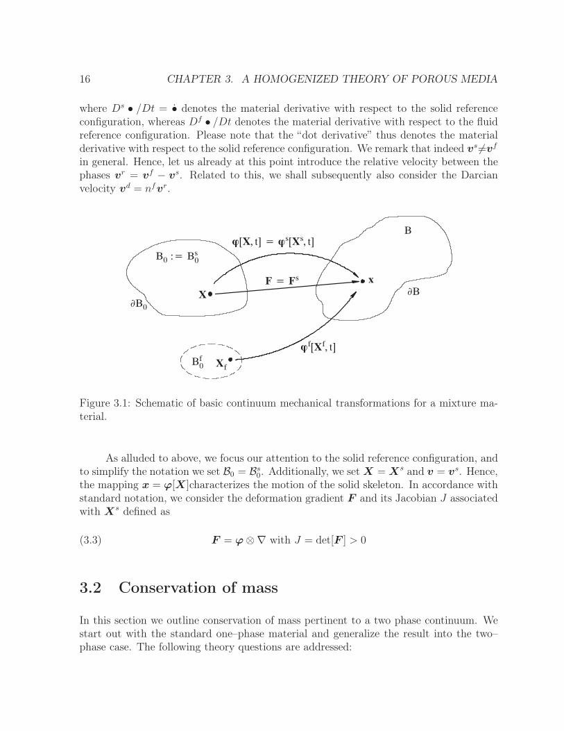
Let us in the following consider our porous material as a homogenized mixture betweensolid and fluid (which may be a liquid or a gas depending on the application) phases asmotivated in the previous section. To this end, we denote the phases s or f , where sstands for the solid phase, whereas f stands for the fluid phase. The representation ofthe porous medium as a mixture of constituents, implies that each spatial point x of thecurrent configuration at the time t are simultaneously occupied by the material particlesXα. We emphasize that the constituents s, f relate to different reference configurations,i.e. Xs 6= Xf , cf. Fig. 3.1. During the deformation these “particles” move to the currentconfiguration via individual deformation maps defined as

(3.1) x = ϕ [Xs] = ϕf[Xf

]

As to the associated velocity fields we have in view of the deformation maps ϕ andϕf the relations

(3.2) vs =Dsϕ[X ]

Dt= ϕ[X ] , vf =

Dfϕf[Xf

]

Dt

15

16 CHAPTER 3. A HOMOGENIZED THEORY OF POROUS MEDIA

where Ds • /Dt = • denotes the material derivative with respect to the solid referenceconfiguration, whereas Df • /Dt denotes the material derivative with respect to the fluidreference configuration. Please note that the “dot derivative” thus denotes the materialderivative with respect to the solid reference configuration. We remark that indeed vs 6=vf

in general. Hence, let us already at this point introduce the relative velocity between thephases vr = vf − vs. Related to this, we shall subsequently also consider the Darcianvelocity vd = nfvr.

[X, t] s[Xs, t]

X

xF Fs

B0 : Bs0

Xf

f[Xf, t]

B

BB0

Bf0

Figure 3.1: Schematic of basic continuum mechanical transformations for a mixture ma-terial.

As alluded to above, we focus our attention to the solid reference configuration, andto simplify the notation we set B0 = Bs0. Additionally, we set X = Xs and v = vs. Hence,the mapping x = ϕ[X]characterizes the motion of the solid skeleton. In accordance withstandard notation, we consider the deformation gradient F and its Jacobian J associatedwith Xs defined as

(3.3) F = ϕ⊗∇ with J = det[F ] > 0

3.2 Conservation of mass

In this section we outline conservation of mass pertinent to a two phase continuum. Westart out with the standard one–phase material and generalize the result into the two–phase case. The following theory questions are addressed:

3.2. CONSERVATION OF MASS 17

1. Formulate the idea of mass conservation pertinent to a one-phase mixture.Generalize this idea of mass conservation to the two-phase mixture. Discussthe main results in terms of the relative velocity between the phases.

2. Describe in words (and some formulas if necessary) the difference be-tween the material derivative ρ = Dρ[x, t]/Dt and the partial derivative∂ρ[x, t]/∂t, where ρ is the density of the material.

3. Formulate the mass balance in terms of internal mass supply. Discuss atypical erosion process.

4. Formulate the mass balance in terms of the compressibility strains. Set ofthe total form of mass balance in terms of the saturation constraint. In viewof this relationship, introduce the issue of incompressibly/compressibilityof the phases in terms of the compressibility strains.

3.2.1 One phase material

To warm up for the subsequent formulation of mass conservation of a two phase material,let us consider the restricted situation of a one-phase material in which case the total massof the solid may be written with respect to current B and reference B0 configurations as

(3.4) M =

∫

B

ρdv =

∫

B0

ρJdV

where in the last equality we used the substitution dv = JdV .

The basic idea behind the formulation of mass conservation is that the mass of theparticles is conserved during deformation, i.e.

(3.5) m0[X] = m[ϕ[X]] ⇔ ρ0dV = ρJdV

where it was used that m = ρdv.

Let us next apply this basic principle to our one phase solid. First, consider theconservation of mass from the direct one phase material written as:

DM

Dt=

D

Dt

∫

B

ρdv =

∫

B0

(

ρJdV + ρ ˙JdV)

=

∫

B0

(

ρJ + ρJ)

︸︷︷︸

M=˙ρJ

dV =

{J

J= ∇ · v} =

∫

B0

(ρ+ ρv ·∇)JdV :=0

(3.6)

or in localized format we obtain

(3.7) M = (ρ+ ρ∇ · v) J = 0


3.2.2 Two phase material

Consider next the situation of two phases of volume fractions ns for the solid phase andnf for the fluid phase. The mass conservation of the two-phase material is now expressedwith respect to the conservation of mass for the individual phases, so that the total massM is expressed as(3.8)

M = Ms+Mf =

∫

Bs

ρsdv+

∫

Bf

ρfdv =

∫

B

nsρsdv+

∫

B

nfρfdv =

∫

B0

MsdV +

∫

B0

MfdV

where Ms and Mf are the solid and fluid contents, respectively, defined as

(3.9) Ms = Jnfρf , Mf = Jnsρs

We thus express the mass conservation for the solid and fluid phases in turn as: Thebalance of mass now follows for the solid phase as

(3.10)Ds

Dt

∫

Bs

ρsdv =Ds

Dt

∫

B

nsρsdv =Ds

Dt

∫

B0

JρsdV =

∫

B0

MsdV = 0

where we used the dot to indicate the rate with respect to the fixed solid reference con-figuration. This leads to the condition

(3.11) Ms = J ˙ρs + ρsJ = J(

˙ρs + ρs∇ · v)

= 0

Hence, the stationarity of the solid content is a representative of mass conservation of thesolid phase.

The balance of mass now follows for the fluid phase as

Df

Dt

∫

Bf

ρfdv =Df

Dt

∫

B

nfρfdvPB=Df

Dt

∫

Bf0

Jf ρfdV =

∫

Bf0

DfJf ρf

DtdV

PF=

∫

B

(Df ρf

Dt+ ρf∇ · vf

)

dv = 0

(3.12)

where the “PF” and the “PB” denotes “Push-Forward” or “Pull-Back” operations. Itshould be noted that in the PB-operation we consider the fluid reference configuration Bf0whereby we have the dependencies ρf = ρf

[ϕf

[Xf

], t]= ρf

[Xf , t

]. Finally, pull-back

to the solid reference configuration yields:

(3.13)∫

B0

(Df ρf

Dt+ ρf∇ · vf

)

JdV = 0


By localization the condition for mass balance of the fluid phase is finally obtainedas

(3.14)Df ρf [x, t]

Dt+ ρf∇ · vf =

∂ρf

∂t+(∇ρf

)· vf + ρf∇ · vf = 0

3.2.3 Mass balance of fluid phase in terms of relative velocity

Upon introducing the relative velocity vr = vf −v the material time derivative pertinentto the fluid phase may be rewritten as

(3.15)Df ρf

Dt=∂ρf

∂t+(∇ρf

)· v +

(∇ρf

)· vr = ˙ρf +

(∇ρf

)· vr

whereby the balance of mass for the fluid phase in (3.14) becomes(3.16)˙ρf+ρf∇·vf+

(∇ρf

)·vr = ˙ρf+ρf∇·v+ρfvr ·∇+

(∇ρf

)·vr = ˙ρf+ρf∇·v+∇·

(ρfvr

)= 0

It is also of interest to consider the fluid mass balance in terms of the fluid contentdefined as

(3.17) Mf = Jρf ⇒ Mf = J(

˙ρf + ρf∇ · v)

whereby the balance relation (3.14) is formulated as

(3.18) Mf + J∇ ·(ρfvr

)= 0

We thus conclude that the mass balance of the fluid phase may be related to thesolid material via the introduction of the relative velocity. Clearly, the special situationof synchronous motion of the phases, i.e. vr = 0, corresponds to stationarity of both Ms

and Mf . This condition is also sometimes named the “local undrained case”.

3.2.4 Mass balance in terms of internal mass supply

We extend the foregoing discussion by introducing the exchange of mass between thephases via the internal mass production/exclusion terms Gs and Gf , which define therates of increase of mass of the phases due to e.g. an erosion process or chemical reactions.These are in turn related to the local counterparts gs and gf defined as

(3.19) Gs =

∫

B

gsdv =

∫

B0

JgsdV,Gf =

∫

B

gfdv =

∫

B0

JgfdV


Hence, we may extended the balance of mass between the individual solid and fluid phasesas:

(3.20)Ds

DtMs = Gs ⇔

∫

B0

MsdV =

∫

B0

JgsdV

(3.21)Df

DtMf = Gf ⇔

∫

B0

(

Mf + J∇ ·(ρfvr

))

dV =

∫

B0

JgfdV

Let us in addition assume that the total mass total mass is conserved i.e. we havethe condition for mass production/exclusion

(3.22)Ds

DtMs +

Df

DtMf = 0 ⇒ Gs +Gf = 0 ⇒ gs + gf = 0

Clearly, the last expression represents the case of an erosion process where “thefirst phase takes mass from the second phase”. The mass balance relationship for theindividual phases thus becomes

Ms = Jgs = −Jgf

Mf + J∇ ·(ρfvr

)= Jgf

(3.23)

where it may be noted that erosion normally means gf = −gs > 0 corresponding to thesituation that the fluid phase “gains” mass from solid phase.

3.2.5 Mass balance - final result

Let us summarize the discussion of mass balances in terms of the total mass conservationas expressed in (3.23). Hence, in view of (3.23) we may formulate the local condition fortotal mass balance as

(3.24) Ms + Mf + J∇ ·(ρfvr

)= 0

where we note that the solid and fluid contents may be expanded in terms of the volumefractions as

(3.25) Ms = Jρs ⇒ Ms = J(

˙ρs + ρs∇ · v)

= Jρs(

ns + ns∇ · v + nsρs

ρs

)

(3.26) Mf = Jρf ⇒ Mf = J(

˙ρf + ρf∇ · v)

= Jρf(

nf + nf∇ · v + nfρf

ρf

)


In addition, let us next introduce the logarithmic compressibility strains εsv for thesolid phase densification and εfv for the fluid phase densification expressed in terms ofintrinsic densities ρs and ρf as

(3.27) εsv = − log

[ρs

ρs0

]

⇒ εsv = −ρs

ρs⇒

ρs

ρs= −εsv

(3.28) εfv = − log

[ρf

ρf0

]

⇒ εfv = −ρf

ρf⇒

ρf

ρf= −εfv

The mass balance relations now becomes in the compressibility strains:

Ms = Jρs (ns + ns∇ · v − nsεsv) = 0

Mf = ρf(nf + nf∇ · v − nf εfv

)= −∇ ·

(ρfvd

)(3.29)

where vd = nfvr was introduced as the Darcian velocity. Rewriting once again oneobtains

nf + nf∇ · v − nf εfv = −1

ρf∇ ·

(ρfvd

)

ns + ns∇ · v − nsεsv = 0

(3.30)

Combination with due consideration to the saturation constraint, i.e. nf + ns = 1;nf + ns = 0, leads to

(3.31) nf + ns+ns∇·v+nf∇·v−nsεsv−nf εfv = ∇ · v − nsεsv − nf εfv = −

1

ρf∇ ·

(ρfvd

)

where we introduced the Darcian velocity defined as vd = nfvr. We emphasize that theissue of “compressibily” relates to the changes of the densities ρs, ρf following a solidparticle ϕ[X, t]. This means, in particular, that ρf = ρf [ϕ[X ], t] at the assessment offluid compressibility. The reason is that the initial density ρf0 relates to B0 (and not Bf0 ).In this context, we conclude that εsv[x, t]:=0 and εfv [x, t]:=0 corresponds the importantsituation of incompressible solid material and incompressible fluid phase materials, respec-tively. However, we may indeed have the situation that e.g. εsv[x, t] 6= 0 and εfv [x, t]:=0,corresponding a compressible solid phase material.


3.3 Balance of momentum

In this section the balance of momentum is addressed. The outline of the developmentsis defined by the theory questions:

1. Formulate the principle of momentum balance in total format. Formulatealso the contribution of momentum from the different phases. Consider, inparticular, the conservation of mass in the formulation.

2. Express the principle of momentum balance with respect to the individualphases. Focus on the solid phase reference configuration via the introduc-tion of the relative velocity. In this, development express the localizedequations of equilibrium for the different phases. Formulate your interpre-tation of the local interaction forces.

3.3.1 Total format

The linear momentum balance of the solid occupying the region B as in Fig. 3.2 maybe written in terms of the “change” in total momentum P in B, and the externally andinternally applied forces F ext and F int. The linear momentum balance relation is specified(as usual) as

(3.32)DP

Dt= F ext +F int

where the (total) forces of the mixture solid are defined as

(3.33) F ext =

∫

∂B

tdΓ =

∫

B

σ · ∇dv , F int =

∫

B

(ρsg + ρfg

)dv

Please, carefully note that t is the total traction vector acting along the external boundary∂B and g is the gravity. The traction vector is related to the total stress tensor σ = σs+σf

via the outward normal vector n as

(3.34) t = σ · n

where σs and σf are the solid and fluid partial stresses, respectively.

In addition to linear momentum balance, angular momentum balance should beconsidered. However, if we restrict to the ordinary non-polar continuum representationthe main result from this consideration is that the total stress (and also the partial stresses)is symmetric, i.e.

(3.35) σ = σt ⇒ σs = (σs)t ,σf =(σf

)t

3.3. BALANCE OF MOMENTUM 23

Ã^ s Ã^ f g

t

x

B[t]

X Xs

B0

B0 B

[X, t]

n

N

vs

vf

Bf0

Xf

f[Xf, t]

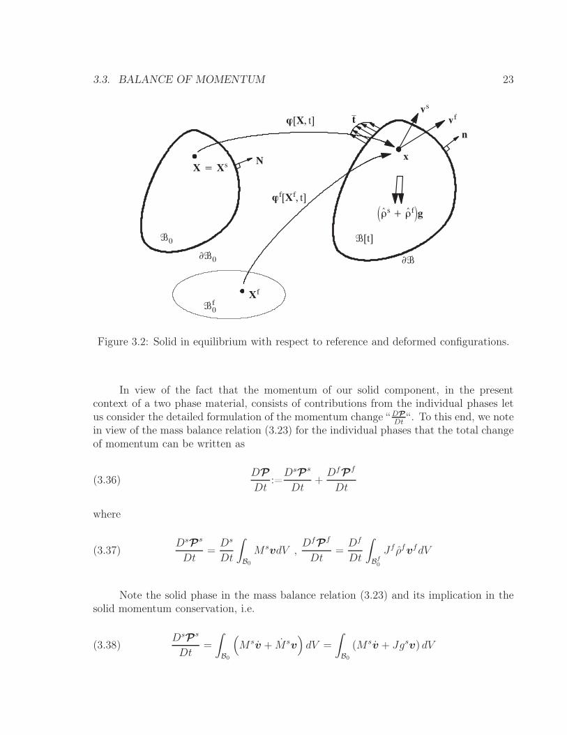
Figure 3.2: Solid in equilibrium with respect to reference and deformed configurations.

In view of the fact that the momentum of our solid component, in the presentcontext of a two phase material, consists of contributions from the individual phases letus consider the detailed formulation of the momentum change “ DP

Dt“. To this end, we note

in view of the mass balance relation (3.23) for the individual phases that the total changeof momentum can be written as

(3.36)DP

Dt:=DsP

s

Dt+DfP

f

Dt

where

(3.37)DsP

s

Dt=Ds

Dt

∫

B0

MsvdV ,DfP

f

Dt=Df

Dt

∫

Bf0

Jf ρfvfdV

Note the solid phase in the mass balance relation (3.23) and its implication in thesolid momentum conservation, i.e.

(3.38)DsP

s

Dt=

∫

B0

(

Msv + Msv)

dV =

∫

B0

(Msv + Jgsv) dV


Likewise, for the fluid phase we obtain the detailed push-forward – pull-back consideration

DfPf

Dt=

∫

Bf0

(

Jf ρfDfvf

Dt+DfJf ρf

Dtvf

)

dV =

∫

Bf0

(

Jf ρfDfvf

Dt+ Jfgfvf

)

dVPF=

∫

B

(

ρfDfvf

Dt+ gfvf

)

dvPB=

∫

B0

(

MfDfvf

Dt+ Jgfvf

)

dV

(3.39)

where the last equality expresses the momentum change with respect to the solid phasematerial reference configuration. In addition, let us also express the fluid accelerationDfvf

Dtin terms of the relative velocity vf = vr + v, whereby the fluid acceleration can be

related to the solid phase material via a convective term involving the relative vr. Thisis formulated via the parametrization vf

[ϕf

[Xf

], t]

as:

(3.40)Dfvf

Dt=∂vf

∂t+ lf · vf =

∂vf

∂t+ lf · v + lf · vr = vf + lf · vr

where lf = vf⊗∇ is the spatial velocity gradient with respect to the fluid motion. Hence,the momentum change may be written as

(3.41)DsP

s

Dt=

∫

B0

(Msv + Jgsv) dV =

∫

B

(ρsv + gsv) dv

DfPf

Dt=

∫

B0

(Mf

(vf +

(vf ⊗∇

)· vr

)+ Jgfvf

)dV =

∫

B

(ρf

(vf + lf · vr

)+ gfvf

)dv

(3.42)

In view of the relations (3.32), (3.33), (3.41) and (3.42), we may finally localize themomentum balance relation for the two phase mixture as

(3.43)DP

Dt= F ext +F int ⇔ σ · ∇+ ρg = ρsvs + ρf

(vf + lf · vr

)+ gfvr ∀x ∈ B

where ρ = ρs + ρg and we made use of the fact that gs + gf = 0 and vr = vf − v.

3.3.2 Individual phases and transfer of momentum change be-

tween phases

As alluded to in the previous sub-section we establish the resulting forces and momentumchanges in terms of contributions from the individual phases, i.e. we have that

(3.44)DP

Dt=DsP

s

Dt+DfP

f

Dt, F ext = F

sext +F

fext , F int = F

sint +F

fint

3.3. BALANCE OF MOMENTUM 25

where

(3.45) Fsext =

∫

B

σs · ∇dv , Ffext =

∫

B

σf · ∇dv , F sint =

∫

B

ρsgdv , Ffint =

∫

B

ρfgdv

Hence, we are led to subdivide the momentum balance relation (3.44) as

(3.46)

DsPs

Dt= F

sint +F

sext +H

s

DfPf

Dt= F

fint +F

fext +H

f

where Hs and H

f are interaction forces due to drag interaction between the phases.These are defined in terms of the local interaction forces hs and hf

(3.47) Hs =

∫

B

hsdv , Hf =

∫

B

hfdv

In addition, it is assumed that the total effect of the interaction forces (or internal rateof momentum supply) will result in no change of the total momentum, i.e. we have that

(3.48) Hs +H

f :=0 ⇒ hs + hf = 0

Hence, we may localize the relation (3.46) along with (3.41) and (3.42) as

(3.49)σs · ∇+ ρsg + hs = ρsv + gsv

σf · ∇+ ρfg + hf = ρf(vf + lf · vr

)+ gfvf

Note that the summation of these relation indeed corresponds to the total form of themomentum balance specified in eq. (3.43).


3.4 Conservation of energy

In this section the conservation of energy is addressed with due consideration to the twoinvolved phases. The developments are defined by the theory questions:

1. Establish the principle of energy conservation of the mixture material. Dis-cuss the involved “elements” and formulate the internal energy and kineticenergy with respect to the solid reference configuration using the relativevelocity.

2. “Work out” the mechanical work rate of the mixture solid.

3. Derive the energy equation using the assumption about an ideal viscousfluid. In this context, define effective stress of Terzaghi. Discuss the inter-pretation of the Terzaghi stress.

3.4.1 Total formulation

Let us first establish the principle of energy conservation (=first law of thermodynamics)written as the balance relation applied to the mixture of solid and fluid phases as

(3.50)DE

Dt+DK

Dt=W +Q

where E = Es+Ef is the total internal energy and K = Ks+Kf is the total kinetic energyof the mixture solid and the total material velocity with respect to the mixture materialis defined as D•

Dt:=Ds•s

Dt+ Df•f

Dt. Moreover, W is the mechanical work rate of the solid and

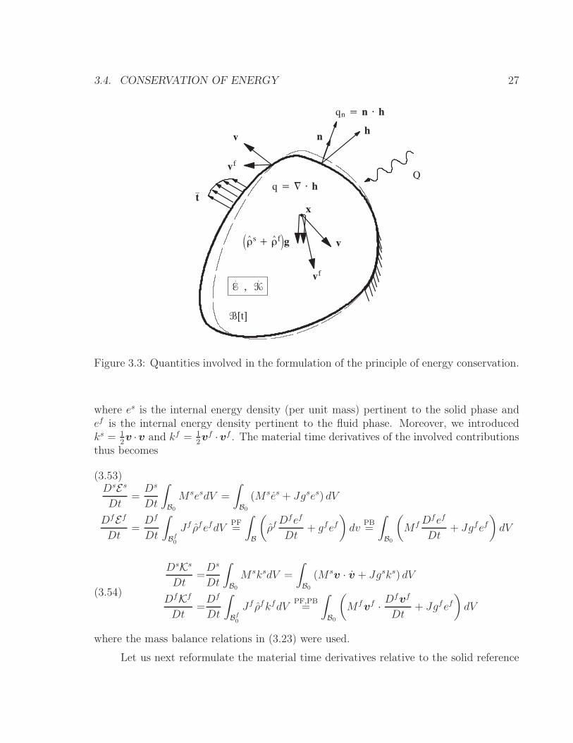
Q is the heat supply to the solid. In the following we shall not disregard Q in the energybalance although we will confine ourselves to isothermal conditions subsequently. Thedifferent “elements” involved in the energy balance are depicted in Fig. 3.3 below.

3.4.2 Formulation in contributions from individual phases

The individual contributions Eα and Kα to the total internal and kinetic energies E , Kare defined as

(3.51) Es =

∫

B

ρsesdv =

∫

B0

MsesdV , Ef =

∫

B

ρfefdv =

∫

Bf0

Jf ρfefdV

(3.52) Ks =

∫

B

ρsksdv =

∫

B0

MsksdV , Kf =

∫

B

ρfkfdv =

∫

Bf0

Jf ρfkfdV

3.4. CONSERVATION OF ENERGY 27

t

Q

E.

, K.

x

n

B[t]

v

vf

Ã^ s Ã^ f g

v

vf

h

q h

qn n h

Figure 3.3: Quantities involved in the formulation of the principle of energy conservation.

where es is the internal energy density (per unit mass) pertinent to the solid phase andef is the internal energy density pertinent to the fluid phase. Moreover, we introducedks = 1

2v ·v and kf = 1

2vf ·vf . The material time derivatives of the involved contributions

thus becomes

DsEs

Dt=Ds

Dt

∫

B0

MsesdV =

∫

B0

(Mses + Jgses) dV

DfEf

Dt=Df

Dt

∫

Bf0

Jf ρfefdVPF=

∫

B

(

ρfDfef

Dt+ gfef

)

dvPB=

∫

B0

(

MfDfef

Dt+ Jgfef

)

dV

(3.53)

DsKs

Dt=Ds

Dt

∫

B0

MsksdV =

∫

B0

(Msv · v + Jgsks) dV

DfKf

Dt=Df

Dt

∫

Bf0

Jf ρfkfdVPF,PB=

∫

B0

(

Mfvf ·Dfvf

Dt+ Jgfef

)

dV

(3.54)

where the mass balance relations in (3.23) were used.

Let us next reformulate the material time derivatives relative to the solid reference


configuration using the relative velocity vr. To this end, it is first noted that

(3.55)Dses

Dt= es ,

Dfef

Dt=∂ef

∂t+(∇ef

)· v +

(∇ef

)· vr = ef +

(∇ef

)· vr

which leads to

DE

Dt+DK

Dt=

∫

B

(ρses + ρf ef + ρf

(∇ef

)· vr + gses + gfef

)dv+

∫

B

(

ρsv · v + ρfvf ·Dfvf

Dt+ gsks + gfkf

)

dv =

∫

B

(

˙e+ ρf(∇ef

)· vr

)

dv+

∫

B

(

ρsv · v + ρfvf ·Dfvf

Dt

)

dv +

∫

B

gf(ef + kf − (es + ks)

)dv

(3.56)

In the last equality we introduced the (solid) material change of internal energy ofthe mixture defined as

(3.57) ˙e = ρses + ρf ef

3.4.3 The mechanical work rate and heat supply to the mixture

solid

In view of Fig. 3.3 we may “work out” the mechanical work rate produced by the gravityforces in B and the forces acting on the external boundary Γ. This is formulated as

W =

∫

B

(ρsg · v + ρfg · vf

)dv +

∫

Γ

(v · (σs · n) + vf ·

(σf · n

))dΓ

DIV=

∫

B

((∇ · σs + ρsg) · v +

(ρfg +∇ · σf

)· vf + σs : l + σf : lf

)dv

(3.58)

where the last expression was obtained using the divergence theorem “DIV” (anda alongwith some additional derivations). Combination of this last relationship with the equilib-rium relations of the phases in eq. (3.49) yields the work rates of our mixture continuumas

W =

∫

B

(

ρs · v · v + ρfDfvf

Dt· vf

)

dv +

∫

B

(σs : l + σf : lf − hf · vr

)dv+

∫

B

(gsv · v + gfvf · vf

)dv

(3.59)


Let us consider next the heat supply Q, cf. Fig. 3.3, to the solid formulated as

(3.60) Q = −

∫

Γ

n · hdΓDIV= −

∫

B

∇ · hdv = −

∫

B

qdv

where the last equality was obtained by using the divergence theorem. We note that h isthe thermal flux vector that transports heat energy from the mixture solid, and q = ∇ ·his the divergence of thermal flow. In particular, we have that q > 0 corresponding toproduction of energy at the material point

3.4.4 Energy equation in localized format

Hence the balance of energy stated in (3.50) along with (3.56), (3.59) and (3.60) can nowbe formulated as

∫

B

˙edv +

∫

B

ρf(ef∇

)· vrdv +

∫

B

gf(ef + kf − (es + ks)

)dv =

∫

B

(σs : l + σf : lf − hf · vr

)dv +

∫

B

gf(vf · vf − v · v

)dv −

∫

B

qdv

(3.61)

In view of (3.61), let us immediately specify the localized format of the energyequation (while noting that ks = 1

2v · v and ks = 1

2vf · vf ) as

˙e+ ρf(∇ef

)· vr + gf

(ef − es

)=

σs : l + σf : lf − hf · vr + gf(kf − ks

)− q

(3.62)

Once again, let us represent the fluid phase term σf : lf in (3.62) to the motion ofthe solid phase. Hence, we rewrite the term σf : lf as

σf : lf =σf : (l + lr) = {σf : lr = ∇ ·(vr · σf

)− vr ·∇ · σf} =

σf : l +∇ ·(vr · σf

)− vr ·∇ · σf =

σf : l +∇ ·(vr · σf

)+ vr ·

(

hf + ρf(

g −Dfvf

Dt

)

− gfvf)(3.63)

where the the equilibrium relation (3.49b) was used once again. Hence, the relation (3.62)is re-established in terms of the total stress σ of the mixture as

˙e+ q + gf(ef − es

)=

(σs + σf

): l+∇ ·

(vr · σf

)+ ρfvr ·

(

g −Dfvf

Dt

)

− ρfvr ·(∇ef

)− gf

1

2vr · vr =

σ : l +∇ ·(vr · σf

)+ ρfvr ·

(

g −Dfvf

Dt−∇ef

)

− gf1

2vr · vr

(3.64)


3.4.5 Assumption about ideal viscous fluid and the effective stress

of Terzaghi

Using the assumption about the ideal viscous fluid, the fluid stress may be represented as

(3.65) σf = nfsf − nfp1

where sf is the intrinsic (normally viscous) portion of the fluid stress and p is the intrinsic

(non-viscous) fluid pressure. We note already at this point that sf is completely devia-toric, and the non-viscous fluid pressure is equal to the total fluid pressure. Nevertheless,we formulate the term ∇ ·

(vr · σf

)of (3.64) as

(3.66)

∇·(vr · σf

)= ∇·

(vd · sf

)−∇·

(

ρfp

ρfvr)

= ∇·(vd · sf

)−p

ρf∇·

(ρfvd

)−ρfvd∇·

(p

ρf

)

where the introduction of the Darcian velocity vd = nfvr is noteworthy. As a result theenergy balance in (3.66) becomes

˙e + gf(ef − es

)=

σ : l +∇ ·(vd · sf

)−

p

ρf∇ ·

(ρfvd

)+

ρfvd ·

(

g −Dfvf

Dt−∇ef −∇ ·

(p

ρf

))

− gf1

2vr · vr

(3.67)

Upon combining the term − p

ρf∇ ·

(ρfvd

)in (3.67) with the balance of mass of the

mixture material in eq. (3.31) we obtain

(3.68) −p

ρf∇ ·

(ρfvd

)= p∇ · v − nspεsv − nfpεfv

leading to


)= σ : l+∇ ·

(vd · sf

)− nspεsv − nfpεfv+

ρfvd ·

(

g −Dfvf

Dt−∇ef −∇ ·

(p

ρf

))

− gf1

2vr · vr

(3.69)

with the effective stress σ of Terzaghi defined as

(3.70) σ = σ + p1

In order to consider the influence of the viscous contribution to the fluid stress wedevelop the term ∇ ·

(vr · sf

)in its indices as

(3.71) ∇k((vd)

j

(sf)

jk) =(ld)

kj

(sf)

kj) +((vd)

j∇k(sf)jk

)= sf : ld + vd ·

(∇ · sf

)


which leads to


)=

(σ − nfsf

): l + nfsf : lf − nspεsv − nfpεfv+

ρfvd ·

(

g −Dfvf

Dt−∇ef −∇ ·

(p

ρf

)

+1

ρf∇ · sf

)

− gf1

2vr · vr

(3.72)

We thus conclude that the effective stress σ − nfsf (and not the partial stress ofthe solid) that is “felt” by the continuum. It should be emphasized, however, that it isnormally assumed that the viscous portion sf of the fluid stress may be neglected, i.e.sf ≈ 0.

Hence, for practical purposes it is desirable to consider the effective stress as theone that controls the "strength" of a porous medium. In soil mechanics, for example,it is commonly accepted that the strength of soil is dependent on the Terzaghi effectivestress. Thereby the "principle" of effective stress of Terzaghi states that the strength ofthe skeleton is an intrinsic property and it does not depend on the fluid pressure. Onecommon engineering argument for its particular expression, e.g. Zienkiewicz et al. [44], isthat instead of taking a typical cut in the porous medium it is more rational to consider"sections" determining the pore water effect through arbitrary surfaces with minimumcontact points of the solid skeleton. It has also been argued that the compressibility ofthe solid material plays a role in the statement of the effective stress. Much thought hasbeen addressed to this hypothesis, and we may refer to de Boer and Ehlers [15], Ladeand de Boer [32] and Bluhm and de Boer [12] for some contributions on this topic. Fromthe above discussion it follows that the constitutive description of the solid matrix shouldinvolve the effective stress rather than the partial stress of the solid.


3.5 Entropy inequality

In this section the entropy inequality pertinent to a two–phase continuum is outlined.The developments of this section are defined by the theory questions:

1. Establish the total entropy and the second law of thermodynamics in thecontext of a two-phase mixture material. On the basis of the involvedmaterial derivatives and principle of mass conservation, express the entropyinequality in terms of the solid reference configuration.

2. Define and discuss the suitable Legendre transformation in internal energy,Helmholtz free energy, temperature and entropy. Represent and localizethe entropy inequality of the mixture material in terms of these quantities.

3. On the basis of the localized entropy for the mixture material, discussthe different components of the dissipation inequality and relate them todissipative mechanics of the mixture material.

3.5.1 Formulation of entropy inequality

Let us next consider the second law of thermodynamics formulated in terms of the totalentropy S written as

(3.73) S =

∫

B

(ρsss + ρfsf

)dv

where ss and sf are the local entropies per unit mass of the solid and fluid phases,respectively. As to the temperature, it is assumed that it is constant, i.e. it is stationary,and in common for both phases, i.e. we have that θ = θs = θf .

The second law of thermodynamics (which is sometimes also named the “ClausiusDuhems Inequality” (CDI), or simply the “entropy inequality”) is now stated as

(3.74)DS

Dt−Qθ > 0

where "DS

Dt" is the total time derivative of our two-phase porous material as we have

discussed extensively (so far) during the course. Moreover, Qθ is the net heat thermalsupply/per temperature unit defined as(3.75)

Qθ = −

∫

Γ

n · h

θdΓ

DIV= −

∫

B

∇·

(h

θ

)

dv = −

∫

B

1

θ(∇·h−h·∇θ)dv = −

∫

B

1

θ(q−h·∇θ)dv

where θ > 0 is the absolute temperature of the medium

3.5. ENTROPY INEQUALITY 33

With due consideration to the balance of mass stated in eq. (3.23) (involving themass transfer factor gf), we develop the total material derivative of the total entropystated in eq. (3.74). Thereby, the total material change of the entropy is obtained as

(3.76)DS

Dt=

∫

B

(

ρsDsss

Dt+ gsss + ρf

Dfsf

Dt+ gfsf

)

dv

In particular, the material time derivative of the fluid is represented in terms of thatof the solid phase (in the usual way), i.e.:

Dsss

Dt= ss

Dfsf

Dt=∂sf

∂t+(∇sf

)· v +

(∇sf

)· vr = sf +

(∇sf

)· vr

(3.77)

which yields the material change of the total entropy in (3.76) as

DS

Dt=

∫

B

(ρsss + ρf sf + ρf

(∇sf

)· vr + gf

(sf − ss

))dv =

∫

B

(

˙s+ ρf(∇sf

)· vr + gf

(sf − ss

))

dv

(3.78)

where ˙s is the saturated entropy change defined as

(3.79) ˙s = ρsss + ρf sf

3.5.2 Legendre transformation between internal energy, free en-

ergy, entropy and temperature

We relate generically the internal energy e, the free energy ψ and the entropy s to eachother via the Legendre transformation

(3.80) e[A, s] = ψ[A, θ] + sθ

where ψ is the Helmholtz free energy (or simply the free energy) representing the storedreversible energy as a function of the internal variables A. We emphasize that the set{s, θ,A} (where θ is the temperature) represents the independent variables in eq. (3.80).As a result the linearized Legendre transformation reads

∂e

∂AA+

∂e

∂ss =

∂ψ

∂AA+

∂ψ

∂θθ + sθ + sθ ⇔

(∂e

∂A−∂ψ

∂A

)

A+

(∂e

∂s− θ

)

s =

(∂ψ

∂θ+ s

)

θ(3.81)


corresponding to the conditions

(3.82)∂e

∂A=∂ψ

∂A, θ =

∂e

∂s, s = −

∂ψ

∂θ

whereby a clear interpretation of the entropy is obtained, i.e. the “entropy” is the sensi-tivity of the free energy with respect to the temperature.

In the following, let us apply the same transformation with respect to the individualphases. Hence, we introduce the relationships for the solid phase

θss = es − ψs ⇒

θss + ssθ = es −∂ψs

∂AA−

∂ψs

∂θθ = es −

∂ψs

∂AA+ ssθ ⇒

θss = es −∂ψs

∂AA

(3.83)

where ψs is the free energy of the solid phase. However, in the following we shall considerthe isothermal condition leading to

(3.84) ˙θss = θss = es − ψs

Likewise, for the fluid phase we introduce the Legendre transformation

(3.85) θsf = ef − ψf ⇒ θDfsf

Dt=Dfef

Dt−Dfψf

Dt= ef − ψf +

(∇sf

)· vr

where ψf is the free energy of the fluid phase.

In addition, let us also consider the saturated entropy ˙s in (3.79). In view of (3.84)and (3.85) one obtains

(3.86) θ ˙s = θρsss + θρf sf = ρses − ρsψs + ρf ef − ρf ψf = ˙e−˙ψ

3.5.3 The entropy inequality - Localization

In view of the relations (3.74),(3.75) and (3.78), the entropy inequality now reads

(3.87)DS

Dt=

∫

B

(

˙s+ ρf(∇(sf

))· vr + gf

(sf − ss

))

dv +

∫

B

1

θ(q − h ·∇θ)dv ≥ 0

It appears that the localized form of the entropy inequality may be written as

(3.88) Dmech +Dther ≥ 0


where we require that the thermal and mechanical portions of the inequality are assumedto the satisfied independently as

(3.89) Dther = −h ·∇θ ≥ 0 ⇒ h = −Kther ·∇θ ⇒ Dther ≥ 0

(3.90) Dmech = θ ˙s+ ρf(∇(θsf

)− sf∇θ

)· vr + gf

(θsf − θss

)+ q ≥ 0

In (3.90), it was used that θ∇sf = ∇(θsf

)− sf∇θ, and in (3.89) the thermal part

of the entropy inequality is immediately satisfied via the introduction of Fourier’s law ofheat conduction, where Kther is the second order positive definite thermal conductivitytensor.

As to the mechanical portion, we develop Dmech in (3.90) using the the Legendretransformations in the sequel (3.86-3.80). As a result we now obtain

(3.91) Dmech = ˙e−˙ψ+ ρf

(∇(ef − ψf

)− sf∇θ

)· vr + gf

(ef − ψf − (es − ψs)

)+ q ≥ 0

Combination with the energy equation (3.72) yields:(σ − nfsf

): l − nspεsv − ρsψs+

nfsf : lf+

− nfpεfv − ρf ψf+

ρfvd ·

(

g −Dfvf

Dt+

1

ρf∇ · sf −∇ψf −∇ ·

(p

ρf

)

− sf∇θ −1

2

gf

ρfvr)

+

gf(−ψf + ψs

)≥ 0

(3.92)

whereby the final result in fact may be interpreted in terms of a number of independentphenomenological mechanisms of the mixture material. In view the appearance of thedifferent terms in (3.92). This is formulated as

(3.93) D = Ds +Dvf +Di +De ≥ 0

where Ds ≥ 0 is the dissipation produced by the (homogenized) solid phase materialconsidered as an independent process of the mixture. The term Dvf ≥ 0 representsthe dissipation developed by the viscous portion of the fluid stress σf . The term Dnvf

represents dissipation in the non-viscous stress response of the fluid. It is assumed thatthis dissipation can be neglected, i.e. Dnvf:=0. The term Di ≥ 0 represents dissipationinduced by “drag"-interaction between the phases. Finally, the term De > 0 representsdissipation motivated by mass transfer between the phases.

Motivated by the entropy inequality (3.92) the different components of the totaldissipation are defined as

(3.94) Ds = σ : l− nspεsv − nsρsψs ≥ 0


(3.95) Dvf = nfsf : lf ≥ 0

(3.96) Dnvf = −nf(

pεfv + ρf ψf)

:=0

Di = −hfe · vd ≥ 0 with

hfe = −ρf(

g −Dfvf

Dt+

1

ρf∇ · sf −∇

(p

ρf

)

−∇ψf − sf∇θ −1

2

gf

ρfvr)

(3.97)

(3.98) De = gf(ψs − ψf

)≥ 0 ⇒ gf

ERO

≥ 0, ψs − ψf ≥ 0

In (3.97), hfe is the effective drag force. Moreover, we introduced Ds ≥ 0 as thedissipation produced by (homogenized) solid phase material, Dvf ≥ 0 is the dissipationdeveloped by viscous portion of the fluid stress σf , Di ≥ 0 represents dissipation inducedby “drag"-interaction between phases, and, finally, De > 0 is the dissipation motivatedby mass transfer between the phases. In addition, from the assumption that the non-viscous portion of the fluid stress response is non-dissipative it immediately follows thatthe argument of ψf is the compressibility strain εfv defined by ψf = ψf

[εfv]

pertinent toa compressible fluid. It then follows from (3.96) that the fluid pressure can be evaluateddirectly from the compressibility εfv via the state ψf

[εfv]

as

(3.99) pεfv + ρf∂ψf

∂εfvεfv = 0 ⇒ p = −ρf

∂ψf

∂εfv

Alternatively, we may consider the constitutive relation in “compliance” form, in whichcase the fluid pressure p is the primary variable that produces the compressibility εfv .

3.5.4 A note on the effective drag force

It is of significant interest to develop the effective drag force hfe in terms of hf = −hs,which is the actual one appearing in the momentum balance of the fluid phase in (3.49b).To this end, we first note that the constitutive relation p = −ρf∂ψf/∂εfv yields the result

−∇

(p

ρf

)

−∇ψf = −1

ρf∇p+

(

p1

(ρf)2−∂ψf

∂εfv

∂εfv∂ρf

)

∇ρf =

{εfv = − log

[ρf

ρf0

]

} = −1

ρf∇p+

(

p1

(ρf )2+∂ψf

∂εfv

1

ρf

)

∇ρf = −1

ρf∇p

(3.100)

Hence, one obtains the effective drag force hfe in (3.97) stated in the form

(3.101) − nfhfe = nf∇ ·(sf − p1

)+ ρf

(

g −Dfvf

Dt

)

− nfsf∇θ −1

2

gf

ρfvr


Let us next assume, firstly, isothermal conditions corresponding to ψf[εfv]⇒ sf =

−∂ψf

∂θ= 0, and, secondly, a non-erosive process gf :=0 which gives

(3.102) − nfhfe = nf∇ ·(sf − p1

)+ ρf

(

g −Dfvf

Dt

)

To arrive at the relation between hfe and hf , let us reconsider the momentum balancerelation (0b) of the fluid phase written as

− hf = σf · ∇ + ρf(

g −Dfvf

Dt

)

=

nf(sf − p1

)·∇+ ρf

(

g −Dfvf

Dt

)

+(sf − p1

)·∇nf − gfvf =

− hfe +(sf − p1

)·∇nf

(3.103)

Hence, the effective drag force is related to the actual one via the relation

(3.104) hf = nfhfe −(sf − p1

)·∇nf

The momentum balance (3.49b) can thus be restated as

(3.105) ρfDfvf

Dt= ∇ · sf −∇p+ hfe + ρfg

which is the momentum balance of the fluid phase represented in intrinsic quantities. Wenote that in this relationship the effective drag force hfe plays the role of the “actual” dragforce.


3.6 Constitutive relations

Guided by the conservation principles formulated for the two-phase mixture, we outlinein this section constitutive relations for the different phase as well as for their interaction.The developments are defined by the theory questions:

1. Derive the state equation for the effective stress in the context of an hyper-elastic material. Formulate also the transformation between our differentstress measures. Carry out the derivation with the restriction to a non-erosive mixture material. What would happen if the material would havebeen erosive?

2. Motivated by the dissipation Di in eq. (3.92), formulate Darcy’slaw as a constitutive representation of the drag interaction betweenthe phases. Discuss under which circumstances we can write: vd =

−k(

∇p− ρf(

g − Dfvf

Dt

))

where k is the (isotropic) permeability con-stant.

3. Formulate the representation of the fluid phase as a gas phase. In thisdevelopment, derive the fluid compressibility!

Guided by the dissipation inequality we outline, in this section, the constitutiverelations of our two-phase continuum. We then consider in turn the different mechanismsoutlined in the sequel (3.98). In the following, we shall assume that the mass productionterm gf = −gs:=0 pertinent to a non-erosive process.

3.6.1 Effective stress response

To arrive at the proper formulation of the effective stress response, let us formulate thedissipation produced by the solid phase for the entire component as

(3.106) Ds =

∫

B

Dsdv =

∫

B0

JDsdV ≥ 0

where the last expression was obtained after pull-back to the solid reference configuration.It may be noted that the integrand JDs in (3.106) may be rewritten in terms of theKirchhoff stress τ = Jσ (and the second Piola Kirchhoff stress S) as

(3.107) JDs = τ : l − nspεsv − Jnsρsψs =1

2S : C − Jnspεsv − ρs0ψ

s

where, in particular, the last equality was obtained from mass conservation due to thestationarity of Ms =Ms

0 = ρs0.

3.6. CONSTITUTIVE RELATIONS 39

Let us for simplicity assume hyper-elasticity “HE”, whereby we obtain the depen-dence ψs [C, εsv] in the free energy for the solid phase. We then have JDs:=0 leadingto

ψs [C, εsv] =∂ψs

∂C: C +

∂ψs

∂εsvεsv ⇒

JDs =1

2

(

S − 2ρs0∂ψs

∂C

)

: C − Jns(

p+ ρs∂ψs

∂εsv

)

εsvHE= 0

(3.108)

We thus obtain the constitutive state equations at hyper-elasticity:

(3.109) S = 2ρs0∂ψs

∂C

(3.110) p = −ρs∂ψs

∂εsv

where S = S − JC−1p is the consequent effective second Piola Kirchhoff stress dueto the Terzahgi effective stress principle, and p is the intrinsic fluid pressure. Like inthe formulation of the fluid compressibility in (3.99), we may alternatively consider theconstitutive relation (3.110) in “compliance” form, whereby (again) the fluid pressure pdrives the solid compressibility εsv.

3.6.2 Solid-fluid interaction

Related to the constitutive relation for the densification of the gas, we consider the modelfor the drag interaction motivated by the dissipation Di in (3.98) written as

(3.111) Di = −hfe · vd ≥ 0

where the effective drag force hfe (or hydraulic gradient with negative sign) is chosen toensure positive dissipation, cf. the representation of Fourier’s law of heat conduction in(3.89), according to the linear Darcy law

(3.112) vd = −K · hfe

where K is the positive definite permeability tensor. To simplify the analysis let us restrictto isotropic permeability conditions using the scalar valued permeability parameter k,whereby K = k1 and k > 0.

Experimental observations shows that the permeability k may be expressed in theeffective gas-fluid viscosity µf and the intrinsic permeability Ks of the solid material.This is written as

(3.113) − hfe =

µf

KSvd ⇒ k =

Ks

µf


Neglecting viscous part of the fluid stress sf in (3.102), we obtain

(3.114) vd = −k

(

∇p− ρf(

g −Dfvf

Dt

))

To conclude the developments in this subsection, we remark that the special situationof “impermeable material” (or closed cells in a cellular material), is named the “undrainedcase”. In this case we have vd:=0 and Di:=0, corresponding to Ks → 0.

3.6.3 Viscous fluid stress response

It appears that the deviatoric fluid stress response sf generates the dissipative portionDvf = nfsf : lf ≥ 0. To ensure positive dissipation, the interpretation of sf is then thatthe corresponding stress response is purely viscous and thereby completely dissipative.This is formulated as

(3.115) sf = 2µfIdev : lf ⇒ Dvf = nfsf : lf = 2µfnf lf : Idev : lf ≥ 0

where µf is the intrinsic fluid viscosity parameter and Idev is the forth order deviatoricprojection operator.

3.6.4 Solid densification - incompressible solid phase

The intrinsic density of the solid phase is normally considered as a constant during thedeformation process of the material. This corresponds to the usual assumption of incom-pressible solid phase material. Hence, we have εsv:=0 and

(3.116) εsv = − log

[ρs

ρs0

]

:=0 ⇒ ρs = ρs0

In addition, for hyper-elasticity we obtain the dependence ψs [C, εsv] → ψs[C] in thefree energy for the solid phase.

3.6.5 Fluid densification - incompressible liquid fluid phase

The intrinsic density of the fluid phase considered as a liquid is also normally consideredas a constant during the deformation process of the mixture material. This correspondsto the usual assumption of incompressible fluid phase material. Hence, we have εfv :=0 and

(3.117) εfv = − log

[ρf

ρf0

]

:=0 ⇒ ρf = ρf0

3.6. CONSTITUTIVE RELATIONS 41

In addition, we obtain the dependence ψf[εfv]→ 0 in the free energy for the fluid

phase.

3.6.6 Fluid phase considered as gas phase

In some applications it is of interest to model the fluid phase considered as a compressiblegas concerning the non-viscous pressure response, e.g. gas-filled foam materials subjectedto large rapid deformations. To this end,the gas-pressure response is modeled using theideal gas law (or the Boyle–Mariotte’s law) written as

(3.118) ρf =mg

Rθp

where R is the universal gas constant, θ is the constant (absolute) temperature and mg

is the molecular mass of the gas. From the basic definition of the compaction of the gasin (3.28) we obtain

(3.119) ρf = ρf0e−ε

fv ⇒ p = p0e

−εfv with p0 =

Rθ

mgρf0

where p0 is the initial gas-pressure (normally considered as the atmospheric pressure). Weremark that the linearized response of the gas phase may be represented as

(3.120) p = −Kf εfv with Kf = p0e−ε

fv

where Kf is the compression modulus of the gas. Indeed, Kf increases when the gas isdensified, e.g. in the extreme case we obtain Kf → ∞ when εfv → −∞.

Hence, in view of (3.99) we find that the stored mechanical energy in the gas phasemay be formulated in terms of the compaction of the gas-phase, i.e. ψf = ψf

[εfv], so that

(3.121)∂ψf

∂εfv= −

p

ρf= −

Rθ

mg

3.6.7 A remark on the intrinsic fluid flow

We note that in view of the constitutive relations (3.113), (3.115) and (3.121) that

(3.122) sf = 2µfIdev : lf , hfe = −µf

KSvd , p = −ρf

∂ψf

∂εfv= {ρf =

mg

Rθp} =

Rθ

mgρf

Upon inserting these relations into (3.105) we obtain corresponding to the compress-

ible Navier-Stokes equation representing the fluid flow in terms of the intrinsic properties.This is formulated as

(3.123) ρfDfvf

Dt= 2µf∇ ·

(Idev : lf

)−Rθ

mg∇ρf −

µf

KSvd + ρfg


3.7 Balance relations for different types of porous me-

dia

In the following subsections we consider a couple of specific porous media specified asspecializations from the developed framework of balance relations of porous media. Inaddition, the governing coupled solutions for the different porous media are formulatedin weak form. The following theory questions define the development of this section:

1. Define and discuss the specialization to the classical incompressible solid-liquid porous medium. Which are the restrictions imposed? Elaborate, inparticular, on the balance of mass in this context. Which are the conditionsimposed on the volume fractions?

2. Formulate the entropy inequality in the context of the incompressible solid-liquid porous medium. Formulate and discuss the relevant constitutiverelations in this context.

3. Set up the governing equations for the incompressible solid-liquid porousmedium. Define the primary solution and establish the weak coupled equa-tions corresponding to this solution.

4. Define and discuss the specialization to the compressible solid-gas medium.Which are the restrictions imposed in this case as compared to the previousone? Elaborate, in particular, on the balance of mass in this context.Which are the conditions imposed on the volume fractions?

5. Set up the governing equations for the compressible solid-gas medium. De-fine the primary solution and establish the weak coupled equations corre-sponding to this solution.

6. Formulate and discuss the consequences of the small solid deformationassumption from the kinematical and constitutive response point of view.

3.7.1 Classical incompressible solid-liquid porous medium

Let us consider as a first prototype the classical incompressible solid-liquid porous medium.To this end, we assume firstly (which was in fact already assumed in the development ofthe constitutive relations) that the medium is non-erosive corresponding to gf = −gs:=0.Secondly, as alluded to in the title, we assume that the phases are incompressible corre-sponding to the compressibility strains

(3.124) εsv:=0 , εfv :=0

3.7. BALANCE RELATIONS FOR DIFFERENT TYPES OF POROUS MEDIA 43

for the solid and the fluid phases, respectively, cf. eqs, (3.27-3.28). Hence, the intrinsicdensities of the phases are stationary, i.e. we have ρs = 0 and ρf = 0 in this case. Thirdlyit is assumed that the dissipative fluid stress is small enough to be neglected, i.e. we setsf :=0.

Balance of mass

In view of the aforementioned restrictions, we conclude in view of the balance of mass in(3.31) of the mixture material that we have for incompressible phases the relationship:

(3.125) ∇ · v = −1

ρf∇ ·

(ρfvd

)

In addition we, of course have the mass balance conditions in (3.23) for the individualphases as usual:

(3.126) Ms = 0 , Mf + J∇ ·(ρfvd

)= 0

which may be elaborated on for the present case of incompressible phases as

Ms = 0 ⇒ nsρsJ = ns0ρs0 ⇒ ns = {ρs = ρs0} =

ns0J

⇒ nsJ + nsJ = 0 ⇒

nf = nsJ

J=

(1− nf

)∇ · v

(3.127)

Hence, we may develop the balance of mass for the fluid phase in (3.126b) as

Mf + J∇ ·(ρfvd

)= J ˙ρf + J ρf + J∇ ·

(ρfvd

)= Jnfρf + J∇ · vρf + J∇ ·

(ρfvd

)=

J(1− nf

)∇ · vρf + Jnf∇ · vρf + J∇ ·

(ρfvd

)= J∇ · vρf + J∇ ·

(ρfvd

)= 0

(3.128)

In view of sequence of developments in (3.128), we thus conclude that the balanceof mass in (3.127) is indeed embedded in balance of mass for the fluid phase. In addition,from the developments in (3.128), we conclude that the conditions for the volume fractionsbased on the assumption of incompressible solid phase can be formulated as:

(3.129) ns =ns0J

, nf =J −

(

1− nf0

)

J⇒ nf = ns

J

J=

(1− nf

)∇ · v


Balance of momentum

As to the balance of momentum, we simply specialize the momentum balance of themixture material in (3.43) from the assumption of a non-erosive material to the equilibriumrelation

(3.130) σ · ∇+ ρg = ρsvs + ρf(vf + lf · vr

)∀x ∈ B

where it may be noted the σ is the total stress which in turn is related to the effective(constitutive) stress σ and the fluid pressure p via the Terzaghi effective stress principlein (3.70), i.e. σ = σ − p1

Entropy inequality of mixture material

Based on the fact that our mixture material can be characterized with respect to theisothermal condition, incompressible phases and non-erosive material, we make the follow-ing restrictions from the general entropy inequality established in the sequel (3.124-3.130)as:

(3.131) ψs[A, θ] → ψs[A] , ψf[εfv , θ

]→ 0 , sf → 0 , gf → 0

We emphasize that this restriction could not have been done prior to the establish-ment of the entropy inequality. We rather make the restriction when the expression ofthe entropy inequality have been fully developed. The specialized entropy inequality isnow reduced to two independent mechanisms, namely, the dissipation produced by theincompressible solid phase considered as a porous skeleton and the interaction betweenthe phases. This is written as

(3.132) Ds ≥ 0 , Di ≥ 0

where

(3.133) Ds = σ : l − nsρsψs ≥ 0 , Di = −hfe · vd ≥ 0

As to the effective drag force, we restrict from the final expression in (3.101) withsf → 0 to the relation

(3.134) hfe = ∇p− ρfg + ρfDfvf

Dt

Concerning the constitutive relations in the present context, we are now guidedby the relation (3.109) to propose for hyperelastic response and isotropic linear Darcyinteraction between the phase the constitutive response:

(3.135) JDs =1

2S : C − ρs0

∂ψs

∂C: C:=0 ⇒ S = 2ρs0

∂ψs

∂C


(3.136) Di = −hfe · vd ≥ 0 ⇒ vd = −khf

e ⇒ vd = −k

(

∇p− ρf(

g −Dfvf

Dt

))

where k is the isotropic solid-liquid permeability parameter, cf. eq. (3.113).

Weak form of governing equations

In order to resolve e.g. the effective stress S and the Darcy flow vd pertinent to astructure problem, we consider the constitutive relations, the balance of mass, the balanceof momentum formulated as a coupled set of relations. In the present case, these coupledrelations may be established with respect to the current configuration B, shown in Fig.3.4, and we formulate the momentum balance of the mixture from (3.130), the balance ofmass for the mixture in (3.128), and the intrinsic fluid Darcy flow in (3.136) as

(σ − p1) · ∇+ ρg =(ρs + ρf

)v + ρf vr + ρf (l+ lr) · vr

∇ · v +1

ρf∇ ·

(ρfvr

)= 0

hfe = ∇p− ρfg + ρfDfvf

Dt=

∇p− ρfg + ρf (v + vr) + ρf (l + lr) · vrDarcy= −

nf

kvr

(3.137)

We identify the primary variables for the coupled problem as the placement x =ϕ[X] ⇒ v = ϕ for the solid particles, the fluid pressure p, and the relative velocity vr,i.e. the primary solution is identified as P = {v, p, vr}.

The idea is then to establish the solution P ∈ V in weak form where V is thefunction space associated with P = {v, p, vr} so that

(3.138) V [w, η,wr] = {w ∈ P, η ∈ S,wr ∈ H}

where in turn P is the function space containing the virtual displacement field w[x], S isthe function space containing the virtual fluid pressure field η[x], and H is the functionspace containing the virtual relative (or seepage) velocity field wr[x].

The coupled set of equations in (3.137) are recast into weak form following thestandard steps: 1) Multiply eqs. (3.137) with the proper virtual field and 2) integrate


t n x

n

B

v

vr

Ã^ s Ã^ f g

vd

Q n vd

Figure 3.4: Current domain along with the mechanical solid-fluid actions.

over the current domain as

∫

B

σ : l[w]dv +

∫

B

(ρs + ρf

)w · vdv +

∫

B

ρfw · vrdv +

∫

B

ρfw · (l+ lr) · vrdv =∫

Γ

w · σ · ndΓ +

∫

B

w · ρgdv

∫

B

ηρf∇ · vdv +

∫

B

η∇ ·(ρfvd

)dv =

∫

B

η∇ · vdv −

∫

B

(∇η) · vddv +

∫

Γ

ηρfvd · ndΓ = 0

∫

B

wr ·∇pdv −

∫

B

ρfwr · gdv +

∫

B

ρfwr · (v + vr) dv+

∫

B

ρfwr · (l + lr) · vrdv +

∫

B

nf

kwr · vrdv = 0

(3.139)

where the last equalities were obtained using the divergence theorem.


Upon introducing the notation:

(3.140) t = σ · n , Q = ρfvd · n

we may (via (3.70) and (3.140)) reestablish eq. (3.139) as

∫

B

(σ − p1) : l[w]dv +

∫

B

(ρs + ρf

)w · vdv +

∫

B

ρfw · vrdv +

∫

B

ρfw · (l + lr) · vrdv =∫

Γ

w · tdΓ +

∫

B

ρw · gdv ∀w ∈ P

∫

B

ηρf∇ · vdv −

∫

B

J −(

1− nf0

)

J(∇η) · vrdv = −

∫

Γ

ηQdΓ ∀η ∈ S

∫

B

wr ·∇pdv +

∫

B

ρfwr · (v + vr) dv +

∫

B

ρfwr · (l + lr) · vrdv+

∫

B

1

k

J −(

1− nf0

)

Jwr · vrdv =

∫

B

ρfwr · gdv ∀wr ∈ H

(3.141)

We emphasize that these relation defines the solution P ∈ V .

3.7.2 Compressible solid-gas medium

Let us consider, as the second prototype, the compressible solid-gas porous medium. Tothis end, like in the previous case, we assume that the medium is non-erosive correspondingto gf = −gs:=0. In addition, it is assumed that the solid phase is incompressible whereasthe fluid phase is compressible, i.e. in view of eqs, (3.27-3.28) we have now

(3.142) εsv:=0 , εfv 6= 0

It is still assumed that the dissipative fluid stress is small enough to be neglected,i.e. sf :=0. In order to model the “fluid” compressibility, the fluid (or gas) phase is hereconsidered as a compressible gas concerning the non-viscous pressure response, e.g. weconsider gas-filled foam materials subjected to large rapid deformations, whereby the gas-pressure response is modeled using the ideal gas law (already specified in (3.121)) writtenas

(3.143) ρf =mg

Rθp = ρf0e

−εfv ⇒ p = p0e

−εfv with p0 =

Rθ

mgρf0


where the last equality was obtained using the definition of the fluid phase compressibilityin (3.28). We also find that from (3.143) that

(3.144)ρf

ρf= −εfv =

mg

Rθ

p

ρf=p

p

Balance of mass

In view of the aforementioned restrictions, we conclude in view of the balance of mass in(3.43) of the mixture material that we have for incompressible phases the relationship:

(3.145) ∇ · v − nf εfv = −1

ρf∇ ·

(ρfvd

)

Let us also in this case elaborate on the mass balance conditions in (3.23) for theindividual phases written as

(3.146) Ms = 0 , Mf + J∇ ·(ρfvd

)= 0

where it is noted that Ms = 0 yields (just as in the case incompressible phases) theconditions

Ms = 0 ⇒ nsρsJ = ns0ρs0 ⇒ ns = {ρs = ρs0} =

ns0J

⇒ nsJ + nsJ = 0 ⇒

nf = nsJ

J=

(1− nf

)∇ · v

(3.147)

Hence, the balance of mass for the fluid phase in (3.146b) may be expanded as

Mf + J∇ ·(ρfvd

)= J ˙ρf + J ρf + J∇ ·

(ρfvd

)=

Jnfρf + Jnf ρf + J∇ · vρf + J∇ ·(ρfvd

)=

J(1− nf

)∇ · vρf + Jnf∇ · vρf + Jnf ρf + J∇ ·

(ρfvd

)=

J∇ · vρf + Jnf ρf + J∇ ·(ρfvd

)= 0

⇒ ∇ · v + nfρf

ρf+

1

ρf∇ ·

(ρfvd

)= 0

(3.148)

which indeed is the balance of mass specified in (3.145). In addition, from the develop-ments in (3.147) and (3.148) we conclude the conditions for the volume fractions from theassumption of incompressible solid phase as:

(3.149) ns =ns0J

, nf =J −

(

1− nf0

)

J⇒ nf = ns

J

J=

(1− nf

)∇ · v


Balance of momentum

Concerning the balance of momentum for the mixture material in (3.43) we obtain, fromthe assumption of a non-erosive material and the fact that the gas density ρf � ρs, theequilibrium relation for the mixture

(3.150) (σ − p1) · ∇+ ρg = ρsvs + ρf(vf + lf · vr

)= ρsvs ∀x ∈ B

where the total stress σ = σ − p1 was directly replaced by the effective (constitutive)stress σ and the fluid pressure p via the Terzaghi effective stress principle in (3.70). Wenote the significant simplification of the inertia forces that can be made as compared tothe previous prototype!

Entropy inequality

In this case we make the following restrictions from the entropy inequality developed inthe sequel (3.94-3.98):

(3.151) ψs[A, θ] → ψs[A] , ψf[εfv , θ

]→ ψf

[εfv]

, sf → 0 , gf → 0

It is emphasized that these restrictions could not have been done prior to the es-tablishment of the entropy inequality! Like in the case of incompressible phases, thespecialized entropy inequality is reduced to two independent mechanisms, i.e.

(3.152) Ds = σ : l − nsρsψs ≥ 0 , Di = −hfe · vd ≥ 0

As to the effective drag force we restrict from the final expression in (3.101) withsf → 0 to the relation

(3.153) hfe = ∇p− ρfg + ρfDfvf

Dt≈ ∇p

where we assumed that ∇p is the dominating term (since ρf is very small).

As to the constitutive relations for the solid phase response we obtain from (3.109)for hyperelastic response and isotropic linear Darcy interaction between the phases theconstitutive response:

JDs =1

2S : C − ρs0

∂ψs

∂C: C:=0 ⇒ S = 2ρs0

∂ψs

∂C

Di = −hfe · vd ≥ 0 ⇒ vd = −khf

e⇒ vd = −k

(

∇p− ρf(

g −Dfvf

Dt

))(3.154)

where k is the isotropic permeability parameter of the solid-gas interaction.



In order to formulate the coupled solid-gas interaction problem we combine the balance ofmass, the balance of momentum and the intrinsic fluid flow as a coupled set of equations.This is formulated with respect to the current configuration B as

(σ − p1) · ∇+ ρsg = ρsv

∇ · v − nf εfv +1

ρf∇ ·

(ρfvd

)= ∇ · v + nf

p

p+

1

ρf∇ ·

(ρfvd

)= 0

hfe = ∇p = −nf

kvr

(3.155)

where the constitutive relation for the gas densification (3.121) was embedded into thebalance of mass. Like in the previous fully incompressible problem, the problem is for-mulated in the solid phase placement x = ϕ[X] ⇒ v = ϕ, the fluid pressure p, and therelative velocity vr. Hence, we formally identify the primary solution as P = {v, p, vr}.However, in the present case the we reduce the problem via simple elimination betweenthe two last equations in (3.155), i.e. we may eliminate the seepage velocity vr so thatP → P = {v, p} and (3.155) is rewritten as

(σ − p1) · ∇+ ρsg = ρsv

∇ · v − nf εfv +1

ρf∇ ·

(ρfvd

)= ∇ · v +

J −(

1− nf0

)

J

p

p−

1

ρf∇ ·

(kρf∇p

)= 0

(3.156)

where the expression for the fluid phase volume fraction nf in (3.149) was inserted in thelast equality.

The relations (3.156) are formulated in weak form so that the solution P ∈ V whereV is a function space defined by

(3.157) V [w, η] = {w ∈ P, η ∈ S}

where in turn P is the function space containing the virtual displacement field w[x], S isthe function space containing the virtual fluid pressure field η[x].

The coupled set of equations in (3.156) are recast into weak form following the steps:Multiply eqs (3.156) with the proper virtual field and integration over the current domain.


This is carried out using the divergence theorem as

∫

B

(σ − p1) : l[w]dv +

∫

B

ρsw · vdv =

∫

Γ

w · σ · ndΓ +

∫

B

w · ρgdv

∫

B

η ρf∇ · vdv +

∫

B

ρfJ −

(

1− nf0

)

Jηp

pdv −

∫

B

η∇ ·(kρf∇p

)dv =

∫

B

ηρf∇ · vdv +

∫

B

ρfJ −

(

1− nf0

)

Jηp

pdv +

∫

B

kρf(∇η) · (∇p)dv +

∫

Γ

ηvd · ndΓ = 0

(3.158)

where the last equation in (3.156) (balance of mass) was premultiplied by the density ρf

prior to the integration in order to avoid the complicated application of the divergencetheorem. Let us also introduce the standard notation for the traction and the normal gasflow on the external boundary, i.e.

(3.159) t = σ · n , Q = ρfvd · n

Hence, in view if (3.158) the solution P ∈ V is established from the coupled set ofrelations:

∫

B

(σ − p1) · l[w]dv +

∫

B

ρsw · vdv =∫

Γ

w · tdΓ +

∫

B

ρsw · gdv ∀w ∈ P

∫

B

ηρf∇ · vdv +

∫

B

ρfJ −

(

1− nf0

)

Jηp

pdv +

∫

B

kρf (∇η) · (∇p)dv =

−

∫

Γ

η QdΓ ∀η ∈ S

(3.160)

3.7.3 Restriction to small solid deformations - Classical incom-

pressible solid-liquid medium

In this subsection, we outline the formulation and consequences of the assumption ofsmall solid deformations pertinent to the classical incompressible solid-liquid medium.We emphasize that the assumption of small deformation concerns merely the solid phaseresponse. As to the fluid response, the assumption of small deformation is of no relevance.

In the case of small solid deformations we make the simplifications: The currentdomain is the same as the solid reference domain, i.e. we have that

(3.161) B → B0 ⇒ ∇X → ∇ , dV → dv


The small deformation solid displacement u is the solid velocity

(3.162) v → u ⇒ l = u⊗∇

whereby the solid spatial velocity gradient becomes equal to the rate of displacementgradient. In addition, the deformation gradient and its Jacobian tends to unity, i.e.

(3.163) F → 1 , J → 1

and the engineering strain rate becomes equal to the linearized Lagrange strain tensor,i.e.

(3.164) ε →1

2C =

1

2

(l + lt

)= (u⊗∇)sym , J = ∇ · v → ∇ · u = 1 : ε = εv

Balance of mass

From (3.125), corresponding to the case of incompressible phases, the mass balance reads

(3.165) εv = −1

ρf∇ ·

(ρfvd

)

In view of (3.127) and (3.128), we now have the conditions for the volume fractions

(3.166) ns = ns0 , nf = nf0 ⇒ nf = nsJ =(1− nf

)εv

Constitutive equations

On the basis of the solid entropy inequality (3.94), we now obtain in the small deformationcase with ψs[C, θ] → ψs[ε] the condition with respect to hyperelasticity

(3.167) Ds = σ : ε− ρs0∂ψs

∂ε: ε:=0 ⇒ σ = ρs0

∂ψs

∂ε

where σ[ε] is now the small deformation effective stress tensor. As a prototype for smalldeformations, we may choose the linear elastic response corresponding to

(3.168) ρs0ψs =

1

2ε : E : ε ⇒ σ = E : ε

where E is the elastic (constant) stiffness modulus tensor.



From (3.141) we now reconsider the governing equations in the context of small deforma-tions as

(σ − p1) · ∇+ ρg =(ρs + ρf

)u+ ρf vr + ρf (l+ lr) · vr

εv +1

ρf∇ ·

(

nf0ρfvr

)

= 0

∇p− ρfg + ρf (v + vr) + ρf (l + lr) · vr = −nf0kvr

(3.169)

corresponding to the weak form with the solution P ∈ V × S ×H written as

∫

B

(σ − p1) · l[w]dv +

∫

B

(ρs + ρf

)w · vdv +

∫

B

ρfw · vrdv +

∫

B

ρfw · (l + lr) · vrdv =∫

Γ

w · tdΓ +

∫

B

w · ρgdv ∀w ∈ V

∫

B

ηρf∇ · vdv −

∫

B

nf0ρf (∇η) · vrdv = −

∫

Γ

ηQdΓ ∀η ∈ S

∫

B

wr ·∇pdv +

∫

B

ρfwr · (v + vr) dv +

∫

B

ρfwr · (l + lr) · vrdv +

∫

B

nf0wr · vrdv =

∫

B

ρfwr · gdv ∀wr ∈ H

(3.170)

3.7.4 Restriction to small solid deformations - Undrained quasi-

static incompressible solid-liquid medium

In this subsection, we outline the formulation and consequences of the assumption ofsmall solid deformations pertinent to the classical quasi-static incompressible solid-liquidmedium at undrained conditions, corresponding to vd := 0. This assumption is of rele-vance for highly impermeable porous materials under “rapid” loading, where the Darcianflow has no time to develop, cf. also the adiabatic thermal flow condition in thermody-namics.

Like in the previous sub-section, in the case of small solid deformations we makethe simplifications: The current domain is the same as the solid reference domain, i.e. wehave that B → B0 ⇒ ∇X → ∇, dV → dv, and the small deformation solid displacementu is the solid velocity v → u ⇒ l = u⊗∇. We also have that the deformation gradient


and its Jacobian tends to unity, i.e. F → 1, J → 1 whereby the engineering strain ratebecomes equal to the linearized Lagrange strain tensor, i.e.

(3.171) ε →1

2C =

1

2

(l + lt

)= (u⊗∇)sym , J = ∇ · v → ∇ · u = 1 : ε = εv

In the undrained situation we have vd := 0, which due to the balance of mass in(3.165) for the completely incompressible case corresponds to the kinematical constraint

(3.172) εv = ∇ · v = 0

In view of (3.166) and (3.172), we now have the conditions for the volume fractionsns = ns0, n

f = nf0 and nf = 0, i.e. the volume fraction are constant in time.

On the basis of the solid entropy inequality (3.167), the small deformation caseψs[C, θ] → ψs[ε] yields the constitutive equation

(3.173) Ds = σ : ε− ρs0∂ψs

∂ε: ε:=0 ⇒ σ = ρs0

∂ψs

∂ε

where σ[ε] is now the small deformation effective stress tensor. As a prototype for smalldeformations, we choose linear elastic response corresponding to

(3.174) ρs0ψs =

1

2ε : E : ε ⇒ σ = E : ε

where E is the elastic (constant) stiffness modulus tensor.

We may now reconsider the governing equations in the present context written as

(σ − p1) · ∇+ ρg = 0

εv = 0(3.175)

corresponding to the weak form with the solution P ∈ V × S written as

∫

B

σ : l[w]dv −

∫

B

p∇ ·wdv =

∫

Γ

w · tdΓ +

∫

B

w · ρgdv ∀w ∈ V∫

B

ρfη∇ · vdv = 0 ∀η ∈ S

(3.176)

whereby it becomes evident that the fluid pressure is nothing by a Lagrangian multiplierfield pertinent to the constraint εv = 0.


A penalized formulation of the undrained case

As an alternative to the formulation out-lined in the previous sub-section, we may considerthe problem of undrained fluid flow conditions reformulated in terms of an incompressiblesolid phase whereas the fluid phase is considered compressible in a fictitious fashion, i.e.it is assumed that εsv := 0 and εfv 6= 0 whereby the balance of mass in view of (3.145)reads

(3.177) ∇ · v − nf εfv = 0

Let us next consider the gas densification in terms of a compressibility modulus kf

defined so that

(3.178) εfv = −p

kf

Clearly, a penalized formulation of (3.177) with respect to the undrained case is obtainedas kf → ∞ leading to εfv → 0 and from (3.178) one obtains ∇·v → 0, corresponding to alimiting undrained situation. Moreover, from (3.177) we also find that the fluid pressurerate p is obtained as

(3.179) p = −kf

nf∇ · v

Upon integrating the fluid pressure rate in time in an implicit fashion we obtain

(3.180) p = np−∆tkf

nf∇ · v

where due to the implicit integration we have ∇ · v = n+1(∇ · v). We thus conclude thatthe coupled u− p problem in (3.176) may be reduced to a pure displacement formulationas

(3.181)∫

B

(

σ[v]−

(

np−∆tkf

nf∇ · v

)

1

)

: l[w]dv =

∫

Γ

w · tdΓ+

∫

B

w · ρgdv ∀w ∈ V

The unknown velocity field v[x] is solved from in a time stepping procedure using theproposed implicit integration in (3.180). The pressure field is then conveniently updatedusing the relation (3.179).


3.8 Numerical procedures - Classical incompressible solid-

liquid porous medium

In this section we outline the numerical solution strategy to the classical incompressiblesolid-liquid porous medium. In particular, the temporal integration of the momentumbalance relations is formulated as an explicit integration step in the spirit of the centraldifference scheme and the forward Euler method. Likewise, the balance of mass is inte-grated using the backward Euler method. The discretization of the problem is proposedand the finite element out-of-balance force vectors are established. It is proposed to re-solve the coupled problem using a staggered solution procedure where the fluid pressureis considered constant over the mechanical step whereas the configuration is consideredfixed over the mass balance step. Finally, a 1D linear assignment problem is outlined.

3.8.1 Temporal integration

In order to integrate in time the coupled boundary value problem we shall consider the twoproblems separated. We thereby consider the time interval I subdivided into a finite setof N time steps so that I =

{0t, .. nt, t, ..N t

}. Typically, as a result of the time integration

procedure we advance the solution step-wise from one time-step nt with known values tothe updated time t = n+1t. In the subsequent representation of the integrated solution,we omit the supscript n+1• for quantities at the updated time tn+1. In this fashion, wemay consider two different types of integration strategies: one explicit integration relatedto the momentum balance relation and another implicit step related to the mass balancerelation.

Momentum balance - Explicit integration step

As the point of departure, let us reconsider the governing balance relations (3.137) restatedwith respect to the reference configuration, whereby these equations are pre-multipliedby the ”J” due to the change of integration domain. Hence, the governing relations arerewritten in terms of the “mechanical problems”

J(τ

J− p1

)

· ∇+(ρs0 +Mf

)g =

(Ms +Mf

)v +Mf vr +Mf (l + lr) · vr

J∇p− Jρfg + Jρf (v + vr) + Jρf (l+ lr) · vr = −Jnf

kvr

(3.182)

and the “mass balance problem” as

(3.183) J∇ · v +J

ρf∇ ·

(ρfvr

)= J +

J

ρf∇ ·

(ρfvr

)= 0

3.8. NUMERICAL PROCEDURES - CLASSICAL INCOMPRESSIBLE SOLID-LIQUID POROUS MEDIUM

Concerning the integration of the mechanical problems (3.182ab) we shall considerthe well known explicit central difference scheme, where the solution is advanced in anexplicit step applied to the (structural) or equilibrium equation. To this end, let us con-sider the central difference scheme applied to the acceleration in the momentum balancerelation (3.182a) whereas a standard forward Euler integration step is proposed formthe relative acceleration vr in (3.182b). This yields the integrated placement ϕ and theintegrated relative velocity vr from the Taylor series expressions

(3.184) ϕ = nϕ+ nv∆t +1

2nv∆t2

(3.185) vr = nvr + nvr∆t

where the “current” solid displacement velocity nv is defined with respect to the currentand the previous time steps as

(3.186) nv :=1

n∆t +∆t

(∆tn∆t

(nϕ− n−1ϕ

)+

n∆t

∆t(ϕ− nϕ)

)

Moreover, in eqs. (3.184) and (3.185) the accelerations nv and nvr are established fromthe “inertia” updated at t = nt written as

(Ms +Mf

)nv =

[

J(τ

J− p1

)

· ∇+(ρs0 +Mf

)g]

t= nt−[Mf nvr +Mf n (l + lr) · nvr

]

t= n∗t

Jρf nvr =

[

−Jnf

knvr − J∇p+ Jρfg

]

−[Jρf

(nv + Jρf n (l + lr) · nvr

)]

t= n∗t

(3.187)

whereby due to the presence of the non-linear convective terms of the inertia the integratedsolution is characterized in an implicit fashion. In practice, the implicit integrated solutioninvolving the convective term n (l+ lr)· nvr is established using a simple fix-point iterationprocedure, as alluded to by the specification t = n∗t in (3.187). However, concerning theestablishment of the placement ϕ in (3.184) we note the explicit character of the integratedsolution, whereby in view of (3.186) it suffices to establish the acceleration at the centralpoint for the advancement of one step. In this advancement, the velocity is nothing butthe mean velocity over the last and the current time-steps (where n∆t is time step-sizeof the last time-step). We also note that the displacement velocity nv implicitly involvesthe current placement.


Mass balance - Implicit integration step

In order to integrate the mass balance relation, we apply backward Euler differences tothe volumetric deformation rate J of the mixture. This is formulated as

(3.188) J '∆J

∆t=J − nJ

∆t

whereby the integrated mass balance relation in (3.183) becomes

(3.189) ∆J +∆tJ

ρf∇ ·

(ρfvr

)= 0

where due to the fully implicit step all the involved variables are established at the updatedtime, e.g. J = n+1J .

3.8.2 Finite element approximations

Placement and displacement fields

Let us next introduce finite element approximations to the solid placement field as ϕ[X],where a finite element subdivision of the region B0 into elements B0e, e=1,..., NEL ismade. It is assumed that each element has the interpolation

ϕ =NODE∑

I=1

N I [X ]ϕI ⇒ w = δϕ =NODE∑

I=1

N I [X ]wI ⇒

l[w] =

NODE∑

I=1

wI ⊗ gI with gI = GI · F−1 and GI =∂N I

∂X

(3.190)

whereN I [X] are the element interpolation functions and ϕI are the corresponding elementnodal placements.

Fluid pressure field

The fluid-pressure field is approximated in the same way, i.e. it is assumed that eachelement has the interpolation

(3.191) p =

NODE∑

I=1

N I [X ]pI ⇒ η =

NODE∑

I=1

N I [X ]ηI ⇒ ∇p

NODE∑

I=1

pIgI ,∇η =

NODE∑

I=1

ηIgI

where pI are the element nodal fluid pressures.


Seepage field

In the present text, we shall consider the seepage field chosen as piecewise constant (withineach B0e) such that

(3.192) vr =

NEL∑

e=1

χe[X]vre ⇒ wr =

NEL∑

e=1

χe[X]wre

where vre is the element seepage (or relative) velocity and χe is defined as

(3.193) χe[X] =

{

1 iff X ∈ B0e

0 otherwise

3.8.3 Finite element equations

Upon inserting the discretization into the weak forms of (3.141) for the momentum andmass balances with due consideration to the temporal integration, we obtain the dis-cretized formulation for the accelerations nv and nvr in (3.187) at the current step ntas

(3.194) M n ˙v + bmec [ nϕ, np] +M conv [vre, vre, v] = 0 with bmec =

NEL

Ae=1

(bmece − f ext

e

)

(3.195) Menve

r + ce = 0 , e = 1, 2, 3...,NEL

where M is the (solid) mass matrix and n ˙v is the displacement vector of the completefinite element structure. We also establish of the integrated mass balance relation (usingimplicit integration in eq. (3.189)) at the updated time n+1t as

(3.196) bmass[ϕ,p] =NEL

Ae=1

bmasse = 0

The involved contributions in the finite element equations (3.194), (3.195) and(3.203) are defined with respect to the mechanical problems (3.194-3.195) in terms ofthe nodal force vectors

(3.197) bmece =

NODE

AI=1

[∫

B0e

(τ − Jp1) · gIdV

]

(3.198) M n ˙v =NEL

Ae=1

(NODE

AI=1

NODE

AJ=1

∫

B0e

(Ms +Mf ) N INJ nvIdV

)


(3.199) M conv =NEL

Ae=1

(NODE

AI=1

∫

B0e

MfN I (vre + (l + lr) · vredV )

)

(3.200) f exte =

NODE

AI=1

[∫

Γ0e

N It1dΓ0 +

∫

B0e

N I(Ms +Mf

)gdV

]

(3.201) Mevre =

∫

B0e

ρfJdV vre

(3.202) ce =

∫

B0e

(

∇p− ρfg + ρf v + ρf(

l + lr +nf [J ]

ρf1

k1

)

· vre

)

JdV

and with respect to the balance of mass (3.203) of the mixture material as

(3.203) bmasse =

NODE

AI=1

[∫

B0e

(−∆tJρfnf [J ]gI · vre + ρfN I∆J

)dV +

∫

Γ0e

∆tN IQdΓ

]

Moreover, conjugated with the nodal vector bmass, we have the structural vector of nodalfluid pressures p. As to the structure of bmass, we note that bmass is the vector of out-of-balance mass transport.

3.8.4 Uncoupled staggered solution strategy

It is noted that the integrated relations (3.194), (3.195) and (3.203) along with the Tay-lor series advancement (3.184-3.185) constitute a coupled set of non-linear finite elementequations, which requires generally requires the proper monolitic coupled solution strat-egy. However, following the work of e.g. Simo and Armero [] applied to thermal problemsand Landervik and Larsson [] applied to compressible solid-gas problems, the idea of thepresent text is to solve the FE-discretized momentum and mass balance relations (3.194-3.195) and (3.203) in an uncoupled staggered fashion. To this end, we shall consider thecase of constant pressure over the mechanical step (corresponding to isothermal split inthe thermal case) whereas the configuration is considered fixed over the mass balancestep.

Constant pressure

The most straightforward formulation of the decoupling is to consider the integration ofthe momentum balance relation with the fluid pressure considered fixed during the time-step. This means that, in the central difference scheme outlined above, we consider in


the evaluation of the acceleration n ˙v with prescribed fluid pressure p = npobtained fromthe previous time step, whereby, pertinent to the central difference scheme, the nodalacceleration n ˙v is established as

n ˙v = −M−1 (bmec [ nϕ, p] +M conv [ nvre,nvre,

n v]) ⇒

ϕ = nϕ+nϕ− n−1ϕ

∆tn∆t +

1

2

(

1 +∆tn∆t

)

n ˙v∆t2(3.204)

(3.205) nvre = −1

Me

ce[nϕ, p, n ˙v, nvre,

nv]⇒ vre =

nvre +nve

r∆t , e = 1, 2, 3...,NEL

where M is the (solid) mass matrix and ϕ is the placement nodal vector of the completefinite element structure. We also emphasize the implicit character of the integrated solu-tion

{n ˙v, nvre} due to the presence of convective terms in the representation of inertia.

It may be remarked that this procedure is in fact consistent with the central differencescheme, where the solution is advanced explicitly at the central point n• with knownsolution quantities at n• and n−1• values, cf. the relations (3.184) and (3.186).

Secondly, the mass balance problem is solved with respect to the fixed placementϕ = const. obtained from the previous mechanical step (3.204)-(3.204), i.e.

(3.206) bmass[p]ϕ=const. = 0

It should be emphasized this relation is generally non-linear in the fluid pressure and thehandling of the problem is described below in sub-section 3.8.4. Note that the coupledproblem becomes reduced to first solving a conventional mechanical step, which generatesinput to mass balance step in form of the mechanical deformation gradient. In turn, themass balance step provides the fluid pressure for the mechanical step.

Handling of non-linear mass balance step

As pointed out in sub-section 3.8.4, the finite element discretized mass balance relationis considered as a separate relation with fixed configuration. The goal is to establish thefluid pressure for the next time-step in the staggered solution procedure by solving forthe fluid pressure in the non-linear relation g[p] defined as

(3.207) g[p] = bmass[p]ϕ=const. = 0

In this relation the nodal force vector bmass due to the mass balance relation is nowexpressed as

bmasse =

NODE

AI=1

[∫

B0e

(∆tJρfnf [J ]gI ·A−1 ·

(∇p− ρfg + ρf ( nv + nvre)

)+

ρfN I∆J)dV +

∫

Γ0e

∆tN IQdΓ

]


In this establishment it was used that the gradient of the pressure is expressed via theeffective drag force and the Darcy law as expressed in (3.137c), i.e.

(3.208) vre = −A−1 ·(∇p− ρfg + ρf ( nv + nvre)

)with A = ρf

(

nl+ nlr +nf [J ]

ρf1

k1

)

where the accelerations nv, nvre and the spatial velocity gradients nl, nlr are consideredknown from the momentum balance step. We also note that A−1 may be interpreted asthe dynamic seepage permeability tensor.

To solve for the pressure p, a standard Newton procedure is used, where, in partic-ular, we consider the linearization of g[p] represented as

(3.209) dg[p] = Kdp , K =NEL

Ae=1

Ke

where the structural Jacobian matrix K is considered as an assembly of element stiffnessmatrices Ke, which in view of (3.203) are given by

(3.210) Ke =NODE

AI=1

NODE

AJ=1

[∫

B0e

∆tJknf [J ]gI · gJdV

]

The condition g = 0 is then resolved as defined by the local Newton iteration in thefluid pressure ip = i−1p+ iξ written as

(3.211){i−1g + dg = i−1g + i−1K iξ = 0

}

i=1,NITE

where NITE is the number of iterations that are required in order to satisfy the tolerance|g| < ε.

Chapter 4

Theory questions and assignment

problems of continuum mechanics of

porous media

4.1 The theory questions

The following theory questions are involved in the course:

Section 2.1:

1. Define and discuss the concept of volume fractions in relation to the micro-constituentsof a two-phase mixture of solid and fluid phases related to an RVE of the body.

2. Define the effective mass in terms of intrinsic and bulk densities of the phases fromequivalence of mass. Discuss the issue of (in)compressibility of the basis of thisdiscussion.

3. Define the effective (representative) velocities of the solid and fluid phases relatedtheir micro–mechanical variations across an RVE. Discuss also the issue of “directaveraging”.

4. Based on the quite general result of stress homogenization of a one-phase material,generalize the result to the two-phase situation. Discuss the partial stresses andtheir relation to intrinsic stresses and micro-stress fields.

Section 3.1:

63

64CHAPTER 4. THEORY QUESTIONS AND ASSIGNMENT PROBLEMS OF CONTINUUM MECHANICS

1. Define and discuss the formulation of the kinematics of a two-phase mixture. In-troduce the different types of material derivatives and formulate and discuss thevelocity fields of the mixture.

2. Prove the formula: J = J∇ · v .

Section 3.2

1. Formulate the idea of mass conservation pertinent to a one-phase mixture. Gen-eralize this idea of mass conservation to the two-phase mixture. Discuss the mainresults in terms of the relative velocity between the phases.

2. Describe in words (and some formulas if necessary) the difference between the ma-terial derivative ρ = Dρ[x, t]/Dt and the partial derivative ∂ρ[x, t]/∂t, where ρ isthe density of the material.

3. Formulate the mass balance in terms of internal mass supply. Discuss a typicalerosion process.

4. Formulate the mass balance in terms of the compressibility strains. Set of thetotal form of mass balance in terms of the saturation constraint. In view of thisrelationship, introduce the issue of incompressibly/compressibility of the phases interms of the compressibility strains.

Section 3.3:

1. Formulate the principle of momentum balance in total format. Formulate also thecontribution of momentum from the different phases. Consider, in particular, theconservation of mass in the formulation.

2. Express the principle of momentum balance with respect to the individual phases.Focus on the solid phase reference configuration via the introduction of the relativevelocity. In this, development express the localized equations of equilibrium for thedifferent phases. Formulate your interpretation of the local interaction forces.

Section 3.4:

1. Establish the principle of energy conservation of the mixture material. Discussthe involved “elements” and formulate the internal energy and kinetic energy withrespect to the solid reference configuration using the relative velocity.

2. “Work out” the mechanical work rate of the mixture solid.

4.1. THE THEORY QUESTIONS 65

3. Derive the energy equation using the assumption about an ideal viscous fluid. Inthis context, define effective stress of Terzaghi. Discuss the interpretation of theTerzaghi stress.

Section 3.5:

1. Establish the total entropy and the second law of thermodynamics in the contextof a two-phase mixture material. On the basis of the involved material derivativesand principle of mass conservation, express the entropy inequality in terms of thesolid reference configuration.

2. Define and discuss the suitable Legendre transformation in internal energy, Helmholtzfree energy, temperature and entropy. Represent and localize the entropy inequalityof the mixture material in terms of these quantities.

3. On the basis of the localized entropy for the mixture material, discuss the differentcomponents of the dissipation inequality and relate them to dissipative mechanicsof the mixture material.

Section 3.6:

1. Derive the state equation for the effective stress in the context of an hyper-elasticmaterial. Formulate also the transformation between our different stress measures.Carry out the derivation with the restriction to a non-erosive mixture material.What would happen if the material would have been erosive?

2. Motivated by the dissipation Di in eq. (3.92), formulate Darcy’s law as a consti-tutive representation of the drag interaction between the phases. Discuss under

which circumstances we can write: vd = −k(

∇p− ρf(

g − Dfvf

Dt

))

where k is the

(isotropic) permeability constant.

3. Formulate the representation of the fluid phase as a gas phase. In this development,derive the fluid compressibility!

Section 3.7:

1. Define and discuss the specialization to the classical incompressible solid-liquidporous medium. Which are the restrictions imposed? Elaborate, in particular,on the balance of mass in this context. Which are the conditions imposed on thevolume fractions?


2. Formulate the entropy inequality in the context of the incompressible solid-liquidporous medium. Formulate and discuss the relevant constitutive relations in thiscontext.

3. Set up the governing equations for the incompressible solid-liquid porous medium.Define the primary solution and establish the weak coupled equations correspondingto this solution.

4. Define and discuss the specialization to the compressible solid-gas medium. Whichare the restrictions imposed in this case as compared to the previous one? Elaborate,in particular, on the balance of mass in this context. Which are the conditionsimposed on the volume fractions?

5. Set up the governing equations for the compressible solid-gas medium. Define theprimary solution and establish the weak coupled equations corresponding to thissolution.

6. Formulate and discuss the consequences of the small solid deformation assumptionfrom the kinematical and constitutive response point of view.

4.2. ASSIGNMENT - UNDRAINED ANALYSIS OF 2D SPECIMEN 67

4.2 Assignment - Undrained analysis of 2D specimen

Consider the solid-fluid undrained 2D specimen in Fig. 4.1. The specimen is loaded witha prescribed velocity r = 2 in the vertical direction acting at the top of the specimen.The effective stress response is assumed to be isotropic elastic, which is represented bythe stiffness modulus tensor

(4.1) E = 2GIsymdev +K1⊗ 1

where G is the elastic shear modulus and K is the elastic bulk modulus. These are furtherdefined in terms of Young’s modulus E and Poisson’s ratio ν written as

(4.2) G =E

2(1 + ν), K =

E

3(1− 2ν)

The actual values of the material and geometry parameters are given in Fig. 4.1.

Two types of formulations of the undrained problem are to be compared in the as-signment. The first one considers the truly incompressible case in terms of a coupleddisplacement-pressure problem as described in the weak form (3.176). The second formu-lation considers a regularized version of the truly undrained case in terms of a compressiblefluid phase, represented by the fluid compressibility parameter kf → ∞, cf. the discussionaround eq. (3.181).

The following subtasks of the assignment are to be considered:

• Formulate the governing equations (including the weak form) pertinent to the undrainedproblem, cf. the discussion in sub-section 3.7.4. The proper formulation of the finiteelement discretization and establishment of coupled FE-equations must be made. Itsuffices to restrict to the well known Taylor-Hood element, with quadratic displace-ments and linear pressure variation with the element.

• Implement the FE-problem in your favorite FE-environment, e.g. Matlab, andresults are to be provided so that the different formulations of the problem canbe compared to each other in terms of the fluid pressure response. Note that in thelimit as kf → ∞, the two formulations should coincide!

• Analyse the effective stress, total stress and fluid pressure distribution in the undrainedspecimen due to the considered prescribed displacement loading. Please note theprescribed displacements at the bottom of the specimen. Discuss why the fluidpressure cannot be prescribed in the present context!

Preliminary results from the analyses are shown in Figs. 4.2, 4.3 and 4.4, corre-sponding to the prescribed displacement r = 2a/10. The results show that the von Mises


r[t]

a

2a

Undrained case1) Lagrangian mult. method2) Penalty method

Parameters

G E2(1 )

K E3(1 2 )

Figure 4.1: Considered undrained 2D–specimen with prescribed displacement loading atthe top and prescribed displacements at the bottom. Set E = 210MPa and ν = 0.15.Concerning the geometry, set a = 50mm.

stress distribution is more or less the same for the different formulations, cf. Fig. 4.2.Concerning the fluid pressure there is a difference, in particular, due to post-processing ofthe pressure distribution. In the incompressible formulation the fluid pressure is obtainedfrom the element nodes from the solution vector, whereas in the compressible formulationthe fluid pressure is obtained at the Gaussian integration point level of the finite elements.

4.3. ASSIGNMENT - WAVE PROPAGATION IN A FLUID SATURATED PILE 69

−0.02 0 0.02 0.04 0.06 0.080

0.02

0.04

0.06

0.08

0.1von Mises stress distribution − Incompressible undrained undrained formulation

x

y

1.5

2

2.5

3

3.5

x 1010

−0.02 0 0.02 0.04 0.06 0.080

0.02

0.04

0.06

0.08

0.1von Mises stress distribution − Compressible undrained formulation

x

y

1.5

2

2.5

3

3.5

x 1010

Figure 4.2: von Mises stress distribution. a) undrained analysis using incompressibleFE-formulation, and b) undrained analysis using compressible FE-formulation

−0.02 0 0.02 0.04 0.06 0.080

0.02

0.04

0.06

0.08

0.1Fliud pressure Distribution − Incompressible undrained formulation

x

y

1

2

3

4

5

6

x 1010

−0.02 0 0.02 0.04 0.06 0.080

0.02

0.04

0.06

0.08

0.1Fluid pressure distribution − Compressible undrained formulation

x

y

1.8

2

2.2

2.4

2.6

2.8

3

3.2x 10

10

Figure 4.3: Fluid pressure distribution. a) undrained analysis using incompressible FE-formulation, and b) undrained analysis using compressible FE-formulation

4.3 Assignment - Wave propagation in a fluid saturated

pile

4.3.1 Problem definitions

Consider the linear 1D pile-problem in Fig. 4.5 subjected to the prescribed velocityv0 = u0 = v (with the initial displacement u0 = u = 0) at the right end, whereas the


−0.02 0 0.02 0.04 0.06 0.080

0.02

0.04

0.06

0.08

0.1Total pressure distribution − Incompressible undrained undrained formulation

x

y

1

2

3

4

5

6

x 1010

−0.02 0 0.02 0.04 0.06 0.080

0.02

0.04

0.06

0.08

0.1Total pressure distribution − Compressible undrained formulation

x

y

1.8

2

2.2

2.4

2.6

2.8

3

3.2x 10

10

Figure 4.4: Total pressure distribution. a) undrained analysis using incompressible FE-formulation, and b) undrained analysis using compressible FE-formulation

left end is considered fixed from the displacement point of view. (The restriction to 1Dis given in sub-section 4.3.2, below.) The fluid pore (excess) pressure is assumed to bezero at the left and the right end of the pile. The constitutive small strain effective stressresponse of the pile material is (for simplicity) assumed to be linear elastic correspondingHooke’s law. A linear Darcy law for the interaction between the phases may also beassumed. This is formulated as

(4.3) σ = Eε , hfe = −nf0kvr

Evaluate the distribution of the effective stress σ[x, t] and the excess fluid pressurep[x, t] of the pile due to the considered dynamic loading consisting of a pulse load P [t], withthe “hold” time th. Utilize the proposed explicit temporal integration procedure for theintegration of the structure finite element problem. Small strains may be assumed. As tothe conservation of mass, the discuss staggered solution procedure involving a mechanicaland mass balance step should be exploited.

In the development of the solution of the problem the 1D pile bar is considereddiscretized into a number of 1D finite elements where the proper solution variables isconsidered discretized. As a part of the assignment, propose the choice of regularity ofthe spatial discretization for the displacement u[x], the fluid pressure p[x] and the seepagevelocity vr[x].

4.3. ASSIGNMENT - WAVE PROPAGATION IN A FLUID SATURATED PILE 71

x

u[x, t]

r[t]

v0 0

u0 0

Lp 0

p 0

E , A , k, nf0 [x, t] , p[x, t]

P[t]P0 if t th0 if t th

Figure 4.5: A 1D wave propagation problem in a fluid saturated pile.

4.3.2 Restriction to 1D

Consider the restriction to the 1D stress state of pile problem given in Fig. 4.5. Theintegration (computational) domain B is then reduced to a 1D interval so that B → [0, L]leading to x → x, dv → Adx, where A is the cross sectional area of the pile. The factthat the stress - strain state is 1-dimensional is represented as

(4.4) σ → σ , l → ε

where σ is the uni-axial stress and ε is the uniaxial strain rate. Likewise the tractiont → σ[L].

As to kinematics we also have that:

u[x] → u[x] , v[x] → v[x] , w[x] → w[x] ,

wr[x] → wr[x] , t → σ[L] , ∇ · v → ε, vr → vr , ∇p→dp

dx

(4.5)

Finally, we may state the weak forms of the governing equations in the context ofour 1D pile-bar problem as

A

∫

L

ε′(σ − p)dx+ A

∫

L

w((ρs + ρf

)v + ρf vr + ρf (l + lr) vr

)dx = A (w[L] σ[L]− w[0] σ[0])

A

∫

L

ρfp′εdv − A

∫

L

ρfnf0dp′

dxvrdx = −A(p′[L]Q[L] − p′[0]Q[0])

A

∫

L

kwrdp

dxdx+ A

∫

L

kρfwr ((v + vr) + (l + lr) vr) dx+ A

∫

L

nf0wrvrdx = 0

(4.6)


Consider the following data for the assignment:

A = 0.2 · 0.2m2 , L = 10m;E = 21GPa , ns = 0.6,

ρf = 1000kgm3

, ρs = 2600kgm3

, k = 1 · 10−7(4.7)

Bibliography

[1] R. Larsson, Continuum mechanics of two-phase porous media, Lecture notes (2006).

[2] S. Toll, A course on micromechanics (2005).

[3] R. de Boer, Theory of Porous Media - Highlights in the Historical Development andCurrent State, Springer Verlag Berlin - Heidelberg - New York, (2000)

[4] O. Coussy, Mechanics of Porous Media, John Wiley & Sons, Chichester, (1995).

[5] F. Armero, Formulation and finite implementation of a multiplicative model of cou-pled poro-plasticity at finite strains under fully saturated conditions, Comput. Meth-ods Appl. Mech. Engrg. 171 (1999) 205-241.

[6] A. Bedford and D.S. Drumheller, Recent advances: Theory of immiscible and struc-tured mixtures, Int. J. Eng. Sci. 21 (1983) 863-960.

[7] M.A. Biot, General theory of three dimensional consolidation, J. Appl. Phys. 12(1941) 155-164.

[8] M.A. Biot, Theory of deformation of a porous viscoelasic anisotropic solid, J. Appl.Phys. 27 (1956) 459-467.

[9] M.A. Biot, Mechanics of deformation and acoustic propagation in porous media, J.Appl. Phys. 33 (1962) 1482-1498.

[10] M.A. Biot, Theory of finite deformation of porous solids, Indiana University Math-ematical Journal 21 (1972) 597-620.

[11] M.A. Biot, Variational Lagrangian-thermodynamics of non-isothermal finite strainmechanics of porous solids and thermomolecular diffusion, Int. J. Solids Structures13 (1977) 579-597.

[12] J. Bluhm and R. de Boer, Effective stresses - a clarification, Arch. Appl. Mech. 66(1996) 479-492.

73

74 BIBLIOGRAPHY

[13] R. de Boer, Highlights in the historical development of the porous media theory:Toward a consistent macroscopic theory, Appl. Mech. Rev. 49 (1996) 201-261.

[14] R. de Boer and W. Ehlers, A historical review of the formulation of porous mediatheories, Acta Mechanica 74 (1988) 1-8.

[15] R. de Boer and W. Ehlers, The development of the concept of effective stresses, ActaMechanica 83 (1989) 77-92.

[16] R.I. Borja and E. Alarcón, A mathematical framework for finite strain elastoplas-tic consolidation Part 1: Balance laws, variational formulation, and linearization.Comput. Meth. Appl. Mech. Engrg. 122 (1995) 145-171.

[17] R.I. Borja, C. Tamagnini and E. Alarcón, Elastoplastic consolidation at finite strainPart 2: Finite element implementation and numerical examples, Comput. Meth.Appl. Mech. Engrg. 159 (1998) 103-122.

[18] R.M. Bowen, Incompressible porous media models by the use of the theory of mix-tures, Int. J. Eng. Sci. 18 (1980) 1129-1148.

[19] R.M. Bowen, Compressible porous media models by the use of the theory of mixtures,Int. J. Eng. Sci. 20 (1982) 697-735.

[20] J.P. Carter, J.R. Booker and J.C. Small, The analysis of finite elasto-plastic consol-idation, Int. J. Num. Anal. Meth. Geomech. 3 (1979) 107-129.

[21] O. Coussy, Thermomechanics of saturated porous solids in finite deformation, Eur.J. Mech (A/Solids) 8 (1989) 1-14.

[22] O. Coussy, Mechanics of Porous Media, John Wiley and Sons, Chichester 1995.

[23] S. Diebels and W. Ehlers, Dynamic analysis of a fully saturated porous mediumaccounting for geometrical and material non-linearities, Int. J. Num. Meth. Engrg.39 (1996) 81-97.

[24] W. Ehlers, On thermodynamics of elasto-plastic porous media, Arch. Mech. 41(1989) 73-93.

[25] W. Ehlers and P. Blome, On porous soil materials saturated with a compressiblepore-fluid mixture. In: W. Ehlers (Hrsg), Beiträge zur Theorie Poröser Medien V,Beiträge zur Jahrestagung der GAMM 1999 in Metz (1999).

[26] W. Ehlers, T. Graf, and M. Ammann, Deformation and localization analysis ofpartially saturated soil. Comput. Methods Appl. Mech. Engrg. 193 2885Ű2910 (2004).

BIBLIOGRAPHY 75

[27] A.C. Eringen and J.D. Ingram, A continuum theory of chemically reacting media-I,Int. J. Engng Sci. 3 (1965) 197-212.

[28] M.A. Goodman and S.C. Cowin, A Continuum theory for granular materials, Arch.Rat. Mech. Anal. 44 (1972) 249-266.

[29] A.E. Green and P.M Naghdi, A dynamical theory of interacting continua, Int. J.Engng. Sci. 3 (1965) 231-241.

[30] P.D. Kelly, A reacting continuum, Int. J. Engng Sci. 2 (1964) 129-153.

[31] P.V. Lade, Instability and liquefaction of granular materials, Computers andGeotechnics 16 (1994) 123-151.

[32] P.V. Lade and R. de Boer, The concept of effective stress for soil, concrete and rock,Geotechnique 47 (1997) 61-78.

[33] J. Larsson, and R. Larsson, Non-linear analysis of nearly saturated porous media- Theoretical and numerical formulation. Comp. Meth. Appl. Mech. Engng. 191,3885-3907 (2002).

[34] R. Larsson, M. Rouhi and M. Wysocki, Free surface flow and preform deformationin composites manufacturing based on porous media theory. European Journal ofMechanics A/Solids 31, 1-12 (2011).

[35] R. Larsson, M. Wysocki and S. Toll, Process modeling of composites using two-phaseporous media theory. European Journal of Mechanics A/Solids. 23, 15-36 (2004).

[36] M. Landervik and R. Larsson, PoreŰgas interaction in foams at finite deformationusing staggered solution techniques. Computer Methods in Applied Mechanics andEngineering, 197 148-159 (2007).

[37] I.-S. Liu, Method of Lagrange Multipliers for Exploitation of the Entropy Principle.Arch. Rat. Mech. Anal. 46, 131-147 (1972).

[38] K. Runesson, On non-linear consolidation of soft clay. Chalmers University of Tech-nology, Dept of Structural Mechanics, Publ. 78:1 (1972).

[39] R. Sandhu and E. Wilson, Finite element analysis of seepage in elastic media, ASCEJ. Eng. Mech. Div. 95 (1969) 641-652.

[40] J.C. Small, J.R. Booker and E.H. Davis, Elasto-plastic consolidation of soil, Int. J.Solids Structures 12 (1976) 431-448.

[41] B. Svendsen and K. Hutter, On the thermodymanics of a mixture of isotropic mate-rials with constraints. Int. J. Engng. Sci. 33 (14), 2021-2054 (1995).

76 BIBLIOGRAPHY

[42] C. Truesdell, Rational Thermodynamics, McGraw-Hill, New York (1969).

[43] C. Truesdell and R. Toupin, Encyclopedia of physics, S. Flugge (Ed.),Vol. III/1,Springer-Verlag, Berlin 1960, pp. 226-793.

[44] O.C. Zienkiewicz, A.H.C. Chan, M. Pastor, B.A. Schrefler and T. Shiomi, Compu-tational geomechanics, John Wiley and Sons, Chichester (1998).

[45] O.C. Zienkiewicz and T. Shiomi, Dynamic behavior of saturated porous media:the generalized Biot formualtions and its numerical solution, Int. J. Num. Anal.Geomech. 8 (1984) 71-96.

Continuum mechanics of two-phase porous media - · PDF fileContinuum mechanics of two-phase...

Documents

Transcript of Continuum mechanics of two-phase porous media - · PDF fileContinuum mechanics of two-phase...