Continuous structured population models for Daphnia

magna

Erica M. Rutter∗, H.T.Banks∗, Gerald LeBlanc@, and Kevin Flores∗∗Center for Research in Scientific Computation

Department of MathematicsNorth Carolina State University

Raleigh, NC 27695and

@Department of Biological SciencesNorth Carolina State University

Raleigh, NC 27695

December 21, 2016

Abstract

We continue our efforts in modeling Daphnia magna, a species of water flea, byproposing a continuously structured population model incorporating density-dependentand density-independent fecundity and mortality rates. Our model is fit to experimen-tal data using the generalized least squares framework and we present confidence in-tervals on parameter estimates. We modify the model to incorporate more complexityinto the density-dependent death rate, but discover that the simpler model outperformsthe more complex model in terms of standard errors and is not inferior to the morecomplex model in terms of information content, using the Akaike Information Criteria.

Key words: continuous structured population models, inverse problems, generalized leastsquares, model selection, information content, residual plots.

1

1 Introduction

Structured population models (SPMs) track the density of a population of individuals overtime with respect to a physiologically structured variable, such as age or size. SPMs havebeen used to describe a wide variety of ecological data, see [16, 17, 20, 29, 23, 24] andthe references therein. SPMs are desirable because they describe the life history of theorganism and allow for dependence of age or density on growth, survival, and fecundityrates. SPMs can be both discretely structured [32] or continuously structured [36].

A continuously structured population model can be preferable to a discrete model forseveral reasons. When using discrete structured population models (SPMs), parameterestimation may be computationally unstable when parameters are time or age-dependent[8, 40]. Previous work [6, 13] has indicated that the Sinko-Streifer model [36], a continuouslystructured population model, is more amenable to estimating age-dependent parametersthan discretely-structured models. Further, we have previously [1] compared discrete andcontinuous SPMs for the density-independent Daphnia magna survival data and found thatthe Sinko-Streifer model generated a better fit to data.

Daphnia magna is a species of water flea widely used in ecotoxicology to assess the haz-ard of chemicals, such as pesticides, on ecosystems, and as a model organism in biomedicalresearch [31, 34, 38, 39]. Ecological risk assessments that use daphnids are most commonlyperformed at the organismal response level. To enable the causal association of organismalresponses to ecosystems adversity, mathematical models are needed to quantitatively con-nect and propagate organismal assessment information to the population level [4, 18, 28].Recent daphnid structured population modeling efforts have lacked age-dependent demo-graphics [25], an estimation of density-dependent parameter uncertainty, or have focusedon qualitative model analysis instead of model validation [19, 21, 22, 26, 30]. Thus, cur-rent daphnia SPMs do not accurately capture the long-term dynamics of aggregate [11]population data.

We propose a continuously structured SPM for Daphnia magna that includes bothdensity-independent and density-dependent growth, fecundity, and mortality. We fit ourmodel to Daphnia magna data using a vector generalized least-squares framework andperform cross-validation. We determine local sensitivities on all estimated parametersto understand how the model is affected by parameter changes. Further, we calculateconfidence intervals and standard errors for our parameters. We also propose a slightvariation on our model, allowing for more flexibility in the relationship between density-dependent mortality and biomass. We estimate the additional parameters and show, usingthe Akaike Information Criteria score, that our simpler model does not perform worse. Wealso obtain realistic confidence intervals using the simpler model.

2

2 Mathematical Model

We employ the Sinko-Streifer equations [36] that describe the continuous-time dynamicsof a population structured over a continuous variable, which in this case we take to be age(a). u(t, a) represents the population at time t of age a.

∂u(t, a)

∂t+∂u(t, a)

∂a= −µind(a)µdep(a,M(t))u(t, a) (1)

The mortality rate is a product of a density-independent rate, µind(a), and a density-dependent rate µdep(a,M(t)). The density-dependent rate depends on age as well as totalbiomass at time t, given by M(t). Our boundary condition represents the introduction ofneonates into the population and is given by:

u(t, 0) =

∫ amax

0kind(s)kdep(M(t− τ))u(t, s)ds (2)

The fecundity kernel in the recruitment term is similarly described by density-independentand density-dependent rates. Following the assumptions validated in previous results [2],the density-dependent rate is delayed and depends on the biomass τ days ago.

We use total population length as a surrogate measure of population biomass, which isgiven by:

M(t) =

∫ amax

0u(t, s)

KM0ers

K +M0(ers − 1)ds. (3)

Based on previous results [2], the length of each daphnid is assumed to follow a logisticgrowth curve.

We assume that the density-dependent rate of mortality is a non-decreasing function

of population biomass, i.e.,∂µdep∂M ≥ 0, and that it is a non-increasing function of age, i.e.,

∂µdep∂a < 0. We use a hill function to describe the effect of age and a linear function to

describe the effect of biomass:

µdep(a,M(t)) = 1 + c1M(t)ch23

ch23 + ah2. (4)

We make the additional assumption that µdep only affects non-reproductive individu-als (size class 1s) and has no affect on reproductive individuals (adults). To model thisassumption, we take c3 = 8 days old (the age just before the first offspring are produced)and the hill coefficient h2 = 10, which describes a sharp cutoff in the age at which densityhas an affect on mortality.

We assume that the density-dependent rate of fecundity is a non-increasing function

of population biomass, i.e.,∂kdep∂M ≤ 0. To model this behavior, we used the following hill

function:

kdep(M(t− τ)) =qh3

qh3 +M(t− τ)h3(5)

3

The density-independent rates of fecundity and mortality were estimated from indi-vidual level data. The daily data for density-independent fecundity was used to directlyparameterize the density-independent fecundity, kind(a), as a function of age. For µind(a),we used an age-varying function that we previously estimated within a density-independentSinko-Streifer framework using piecewise linear splines [7, 1].

The observables for the data set we collected are the total counts of daphnids withintwo size classes, which are described by an age cutoff a1 that we previously determined byestimating the relationship between age and size [2]:

S1(t) =

∫ a1

0u(t, s)ds (6)

S2(t) =

∫ amax

a1

u(t, s)ds (7)

The total population size is the sum of S1(t) and S2(t), or

N(t) =

∫ amax

0u(t, s)ds (8)

The integral in these population counts ends at a specified age, amax, which we taketo be 90 days. This limit is older than the last surviving daphnid we found in density-independent experiments, and allows for finitely defined age-mesh in the numerical PDEsolver.

3 Methods

3.1 Data

The data used to fit our model are obtained as previously described [2], but we will brieflydescribe the data for completeness. A longitudinal study was performed, in duplicate, over102 days. The daphnid media, reconstituted from deionized water as previously described[5], was seeded with five 6-day old female daphnids. Daphnids were counted every Monday,Wednesday and Friday for the first three weeks of the experiment and weekly thereafter.Daphnia were separated into two size classes with a fine mesh 1.62-mm pore size net.

3.2 Generalized Least Squares Parameter Estimation and Uncertainties

In order to fit the model to our available data, we use a vector generalized least squares(GLS) approach outlined in [11, 12]. We calculate the total number of daphnids in each sizeclass: size class one is S1(t, θ) =

∫ a10 u(t, s)ds and size class two is S2(t, θ) =

∫ amaxa1

u(t, s)ds.Our forward solution observations for a set of parameters θθθ is given by the vector fff(t, θθθ) =[S1(t, θθθ), S2(t, θθθ)]

T .

4

The statistical model we consider allows proportional errors and has the form (here Nis the number of observations)

YYY j = fff(tj ;θθθ) + fffγ(tj ;θθθ)Ej , j = 1, 2, ..., N, (9)

where Ej are independent and identically distributed (i.i.d.) with zero mean and covarianceV0 = diag(σ201, σ

202). We estimate our parameters by seeking to minimizing a weighted least

squaresN∑j=1

wwwj [yyyj − fff(tj ;θθθ)]2 (10)

where yyyj are the data and the weights wwwj depend on θθθ. This leads to the so-called gener-alized least squares (GLS) formulation defined by the solution to the normal equations

N∑j=1

[yyyj − fff(tj ;θθθ)]TV −1(tj ;θθθ)∇θkfff(tj ;θθθ) = 0, k = 1, .., κθ, (11)

where κθ is the number of parameters being estimated. We define

V (tj ;θθθ) = diag(f1(tj ;θθθ)

2γ1 σ201, f2(tj ;θθθ)2γ2 σ202

)(12)

and

σ20i =1

N − p

N∑j=1

(yij − fi(tj ;θθθ)fi(tj ;θθθ)γi

)2

, i = 1, 2, (13)

-see Sections 3.2.5 and 3.2.6 of [11]. The iterative algorithm we use is further explained in[11, 12]. We note that in the case of γ = 0, this reduces to the vectorized weighted leastsquares.

Using asymptotic theory [12, 11], the vector generalized least-squares (GLS) estimatorhas a limiting distribution: θθθGLS ∼ N (θθθ0,Σ

N0 ) using the true parameter values θθθ0. Since

these are unknown, we can approximate using our estimated parameter vector, θθθ, andobtain θθθGLS ∼ N (θθθ0,Σ

N0 ) ≈ N (θθθ, ΣN ) where

ΣN ≈

N∑j=1

DTj (θθθ)V (tj ; θθθ)Dj(θθθ)

−1

(14)

with

Dj =

∂f1(tj ;θθθ)∂θ1

...∂f1(tj ;θθθ)∂θκθ

∂f2(tj ;θθθ)∂θ1

...∂f2(tj ;θθθ)∂θκθ

.

and V (tj ;θθθ) as defined above. We use our optimized estimates θθθ from equations (11). Fromthis distribution, we can obtain standard errors and 95% confidence intervals to quantify

5

the uncertainty in the estimation of each parameter. Standard errors for each parameter

i are given by SE(θi) =√

ΣNii . These standard errors [12] are then used to create a 95%

confidence interval around each parameter as [θi − 1.96SE(θi), θi + 1.96SE(θi)].In order to determine the correct statistical error model, in terms of which value of

γ to use, we look towards finite differencing of the data as previously described in [9].The advantage of this method is that we are able to examine psuedo-error residuals withrespect to time and do not introduce bias associated with model error. We examine thesecond-order differencing of the data (the so-called pseudo errors discussed in [9])

εi =1√6

(yi+1 − 2yi + yi−1) (15)

From this estimation of measurement errors, we then can define our modified pseudo-errorsby:

η =εi

|yi − εi|γ. (16)

Here γ = 0 corresponds to vector ordinary least squares and γ 6= 0 represents generalizedleast squares. We separate our replicate data into size classes 1 and 2 and calculated themodified residuals using Eq. (16) for various values of γ.

0 50 100

−100

0

100

Replicate 1 − Size Class 1γ=0.0

0 50 100−5

0

5

γ=1.0

0 50 100−200

0

200

Replicate 2 − Size Class 1γ=0.0

0 50 100−2

0

2

γ=1.0

Res

idua

l

0 50 100−10

0

10

γ=0.5

0 50 100

−100

1020

Time (Days)

γ=0.5 0 50 100

−50

0

50

Replicate 1 − Size Class 2γ=0.0

Res

idua

l

0 50 100−5

0

5

γ=0.5

0 50 100−0.5

0

0.5γ=1.0

0 50 100

−50

0

50

Replicate 2 − Size Class 2γ=0.0

0 50 100

−5

0

5

γ=0.5

0 50 100

−0.5

0

0.5

1

γ=1.0

Time (days)

Figure 1: Modified residuals calculated by Eq. (16). Each column represents either sizeclass 1 (left) or size class two (right). Each row increases values of γ.

Figure 1 shows the modified residuals for each replicate for both the size classes 1 and 2populations. The best statistical model is chosen for plots where the distribution of points

6

appears random. We note that for the size class 1, the juveniles, a value of γ = 0.5 appearsto be the most random. We reject γ = 0 for size class 1 because the magnitude of theresiduals appear to be correlated with time. For size class 2, the adult population, however,γ = 0 is sufficiently random. We note that other works have incorporated varying γ valuesfor certain classes of observables [14, 10].

We only optimize over a subset of our parameter space. Parameters K, r, and M0

describe how individual daphnids contribute to the population biomass, i.e., total lengthM(t), as described in equation (3). The information for these parameters is given in Table1. Due to the small variance, we use the r, K, and M0 parameters from Table 1 forall daphnids. The remaining fixed parameters for the model are given in Table 2. Theparameters in the hill function describing the density-dependent death rate (equation (4))for size class 1s include the age at which the density dependent falls to 0 for 8-day olddaphnids (c3) very steeply (h2). For the parameters in the density-dependent fecundityrate (equation (5)), only h3, the power of the hill function, is fixed.

Parameter K r M0

Fixed effect mean value 3.7346 0.0157 .7333Random effect variance 0.0010533 0.0048239 6.8978×10−7

Table 1: Mean parameter estimates and variances along with individual daphnid parameterestimates for the logistic equation using a nonlinear mixed effects model.

The parameters that are optimized via the above vector generalized least-squares frame-work are τ , the time delay for the effect of density on fecundity, q, the half-maximum forthe effect of density on fecundity, and c1, the slope of the linear relationship betweendensity-dependent mortality and total mass, M(t).

The model equations are solved numerically in MATLAB using the hpde package [35].In order to perform the optimization, we will need an initial guess for MATLAB’s lsqnon-lin. We use direct search [27], a non-gradient-based algorithm, in order to obtain a suitableinitial guess. Direct search requires upper and lower limits for the parameters, which wechoose to be 10−10 and 1000, respectively. The optimization is performed until parametervalues change by less than 0.1%.

Parameter Value

a1 3 daysc3 8 daysh2 10h3 2

Table 2: Fixed parameter values for the model

7

3.3 Cross validation

Previous work indicated that τ > 6 provided the best fit to population data [2]. Here weperform a cross-validation over our two replicates to determine the best value of τ to usein our optimization. We allow τ to vary in integer values from 6 to 24. Integer values werechosen because of the prohibitive computational costs associated with a finer grid.

If we look over our entire data domain D = {d1, d2}, where each di is our replicatedata, our best fit for a given value of τ is generated by the parameters θ = (q, c1) thatminimize the residual sum of squares (RSS) and has a value Rfit:

Rfit(τ) = minθ

[RSS(D, θ, τ)] (17)

θ(τ) = argminθ

[RSS(D, θ, τ)] (18)

Since we have two replicates of data, we can independently determine the parameteroptimizations on each data set:

θi(τ) = argminθ

[RSS(di, θ, τ)] (19)

With these new optimized parameters θi, we compute RSS(D, θi, τ) which represents theerror generated over the full domain D using the parameter estimate θi for a specific valueof τ . We then generate:

Ri(τ) = −N2

ln(2π) + ln(RSS(D, θi, τ)− 1) (20)

where N is the total number of observation points in D. Once these are computed for eachreplicate, our cross validation score for a value of τ is the average of these quantities:

RCrossV al(τ) =1

2

2∑i=1

Ri(τ) (21)

The value of τ the maximizes equation (21) will be used in our simulations.

4 Results

4.1 Cross-Validation

Figure 2 shows the result for the cross-validation scores (equation (21)) for integer valuesof τ , the density-dependent fecundity delay parameter, ranging from 6 days to 24 days.We can see that the maximum cross-validation score is generated for τ = 17 days. Theremaining figures and results use this value of τ .

8

6 8 10 12 14 16 18 20 22 24−290

−285

−280

−275

−270

−265

−260

τ

Cro

ss V

alid

atio

n Sc

ore

Figure 2: Cross validation scores using the two replicates for various integer values of τ ,the fecundity delay parameter. τ = 17 days provides the best cross-validation score.

9

0 12 3

050

1000

500

1000

Age (days)Time (days)

Size

cla

ss 1

0 5 10 15 20

050

1000

50

100

Age (days)Time (days)

Size

cla

ss 2

0 20 40 60 80 1000

500

1000

1500

Time (days)

Size

cla

ss 1

0 20 40 60 80 1000

200

400

600

Time (days)

Size

cla

ss 2

0 20 40 60 80 1000

500

1000

1500

Time (days)

Tota

l pop

ulat

ion

0 5 10 15 20

050

100

0

200

400

Age (days)Time (days)

Tota

l pop

ulat

ion

Figure 3: Density-dependent SPM fit to data for replicate 1. Daphnids separated into sizeclass one (top), size class 2 (middle) and total population (bottom). On the left, the totalnumber of daphnids in each size class per day, on the right a surface representing age, timeand population number.

4.2 SPM Parameter Estimation and Uncertainty

Figure 3 displays the density-dependent SPM fit to the data for replicate 1 with optimizedparameters. The fits are broken up into each size class as well as the total population. Onthe left side are the total population numbers at each day for each class and on the right isa surface representing dynamics of age, time, and population number. The data is shownwith open circles and the model fit in a solid black line. The model solution for replicateone appears to fit each size class as well as the total population.

A similar plot for replicate 2 is shown in Figure 4. We can see that in replicate 2, theoptimized fit does not appear as accurate, especially with size class one during the earlyportion of the simulation. During this time, we can see that there is a sharp increase insize class one, which is even higher than the similar increase in replicate 1. Size class two,however, does appear to have an accurate fit.

The resulting parameters, their confidence intervals, and standard errors are in Table 3,separated into the first replicate (top) and second replicate (bottom). We note that all pa-rameters have non-negative confidence intervals, which we require for biological relevance.

10

0 1 2 3 4

050

1000

500

1000

Age (days)Time (days)

Size

cla

ss 1

0 5 10 15 20

050

1000

50

100

Age (days)Time (days)

Size

cla

ss 2

0 20 40 60 80 1000

500

1000

1500

Time (days)

Size

cla

ss 1

0 20 40 60 80 1000

100

200

300

400

500

Time (days)

Size

cla

ss 2

0 20 40 60 80 1000

500

1000

1500

2000

Time (days)

Tota

l pop

ulat

ion

0 5 10 15 20

050

100

0

200

400

Age (days)Time (days)

Tota

l pop

ulat

ion

Figure 4: Density-dependent SPM fit to data for replicate 2. Daphnids separated into sizeclass one (top), size class 2 (middle) and total population (bottom). On the left, the totalnumber of daphnids in each size class per day, on the right a surface representing age, timeand population number.

The standard errors are relatively small. Although the optimized parameter q for replicate2 is outside the range of the 95% confidence interval generated in replicate 1, the optimizedparameter q for replicate 1 is inside the range of the 95% confidence interval generated inreplicate 2. The parameter c1 for each replicate remains outside of the others’ confidenceinterval. Additional replicates would be useful in determining which set of parameters ismore descriptive of population dynamics.

We would also like to examine the residuals for each replicate with respect to time andmodel value. This will help to insure that the statistical model chosen, of γ = 0.5 for sizeclass 1 and γ = 0 for size class 2, is correct. Figure 5 displays the residuals for both replicateone (left) and replicate two (right). Within each subfigure, the left panels show residualsagainst time and the right panels show residuals against model value. The top figuresrepresent size class one and the bottom figures represent size class two. The residualsfor all cases appear to be evenly distributed, indicating that the choice of statistical errormodel is correct.

11

Parameter Estimate (Rep1) 95% CI (Rep1) SE (Rep1)

q 105.0066 ( 78.0305 , 131.9826) 13.8339c1 0.0142 ( 0.0128, 0.0156 ) 7.0377e-4

Parameter Estimate (Rep2) 95% CI (Rep2) SE (Rep2)

q 145.2262 ( 92.1917 , 198.2607 ) 27.1972c1 0.0191 ( 0.0170 , 0.0212 ) 0.0011

Table 3: Optimal parameters, confidence intervals, and standard errors for replicates 1 and2.

0 50 100−300

−200

−100

0

100

Time (days)0 500 1000

−300

−200

−100

0

100

Model

0 50 100−200

−100

0

100

200

Time (days)0 200 400 600

−200

−100

0

100

200

Model

0 50 100−300

−200

−100

0

100

Time (days)0 500 1000

−300

−200

−100

0

100

Model

0 50 100−100

−50

0

50

100

150

Time (days)0 100 200 300 400

−100

−50

0

50

100

150

Model

Figure 5: Residual plots for replicate one (right) and replicate two (left) for each class sizeand against time and model value. Residuals appear random, implying the statistical errormodel is sufficient.

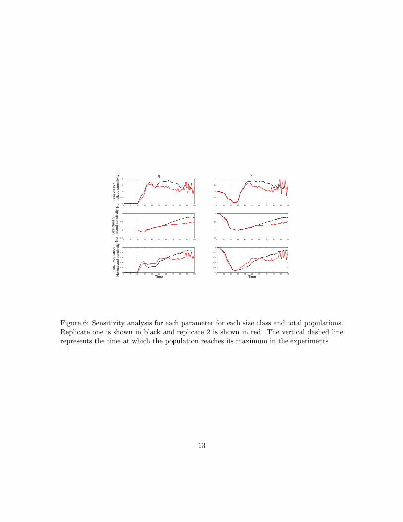
4.3 Sensitivity Analysis

We perform a local sensitivity analysis for the parameters for each replicate and each sizeclass as well as the full population size. Figure 6 displays the results of this sensitivityanalysis. Replicate one is shown in black and replicate two is shown in red. The verticaldashed line is the time at which the daphnia population reaches it’s peak during theexperiments and occurs at the same time for both replicates. Sensitivities were calculatedusing the complex-step method [33] and were corroborated with the finite-differencing.

The left panels of Figure 6 display the sensitivity of q, which is present in the density-dependent fecundity rate (equation (5)). Increasing q leads to higher fecundity rates and,thus, higher population levels for all size classes. Since q is heavily involved in the fecundityrate, it is sensible that there are slight oscillations in the sensitivities, since the daphniagive birth every third day, meaning that those days may be more sensitive to changes inparameter q. We varied our adjoint step size to ensure that the sensitivities converged andthe oscillations were not due to numerical instability.

12

0 10 20 30 40 50 60 70 80 90 1000

0.5

1

1.5

2

Size

cla

ss 1

Nor

mal

ized

sen

sitiv

ity q

0 10 20 30 40 50 60 70 80 90 100−0.5

0

0.5

1

Size

cla

ss 2

Nor

mal

ized

sen

sitiv

ity

0 10 20 30 40 50 60 70 80 90 1000

0.2

0.4

0.6

0.8

1

Time

Tota

l Pop

ulat

ion

Nor

mal

ized

sen

sitiv

ity

0 10 20 30 40 50 60 70 80 90 100−1

−0.5

0

0.5

1

c1

0 10 20 30 40 50 60 70 80 90 100−1.5

−1

−0.5

0

0 10 20 30 40 50 60 70 80 90 100−1

−0.8

−0.6

−0.4

−0.2

0

Time

Figure 6: Sensitivity analysis for each parameter for each size class and total populations.Replicate one is shown in black and replicate 2 is shown in red. The vertical dashed linerepresents the time at which the population reaches its maximum in the experiments

13

The right panels in Figure 6 show the sensitivity of c1. The parameter c1 is the linearrelationship between density-dependent mortality and biomass, M(t) (equation (4)). Forthe total population size, we see that increasing c1 results in lower population levels, whichis sensible, as it increases the density-dependent death rate. However, the dynamics arevery different depending on whether we are looking at size class 1 or size class 2. For sizeclass 1, increasing c1 results in lower size class 1 populations for approximately the first 30days of the experiment, after which increasing c1 results in higher size class 1 populations.This is also somewhat intuitive since populations of size class 1s are very large in the first30 days, meaning that the biomass is quite large, which increases the death rate. However,in later times, population levels are low, which means that increasing c1 may not be enoughto overcome the small values of M(t).

In general, the sensitivities for replicate 1 and replicate 2 have similar overall shapes,although replicate 2 tends to show more oscillatory behavior.

4.4 Model Comparison

In addition to our current model, we also proposed a slight variation in the density-dependent death term, changing the linear relationship between biomass and density-dependent death rate to a hill function. This results in changing equation (4) to

µdep(a,M(t)) = 1 +c1M(t)h1

ch12 +M(t)h1

ch23ch23 + ah2

. (22)

where c2 and h1 are optimized along with q and c1. This change allows further range offlexibility in how the density-dependent death rate depends on the total biomass, M(t).

We perform the same optimization as outlined above including calculating the cross-validation score, optimizing parameters, and determining confidence intervals. We obtaina similar cross-validation, with τ = 16 days being the optimal τ , maximizing equation (21).The resulting optimal parameter fits are displayed in Figures 7 and 8 for replicates 1 and2, respectively.

By eye, the fits to data for the linear density-dependent death rate and the hill functiondensity-dependent death rate appear similar. The optimized parameters for the hill func-tion density-dependent death rate are given in Table 4. We see that our estimates for qare similar to the 2-parameter model. However, when we examine the confidence intervalsand the standard errors, we can see a large decrease in performance from the 2-parametermodel. Three of the four parameters for replicate one have confidence intervals whichcontain negative values, which is not biologically feasible. For replicate two, there are twoparameters which also contain negative values.

It appears that by incorporating the hill function, we are over-parameterizing our model.This is corroborated by examining how the density-dependent death rate, equation (22),behaves with the optimized parameters in Table 4. For replicate one, the optimal parame-ters generate a linear relationship with respect to the biomass, M(t), which explains why

14

0 1 2 3

050

1000

500

1000

Age (days)Time (days)

Size

cla

ss 1

0 5 10 15 20

050

1000

50

100

Age (days)Time (days)

Size

cla

ss 2

0 20 40 60 80 1000

500

1000

1500

Time (days)

Size

cla

ss 1

0 20 40 60 80 1000

200

400

600

Time (days)

Size

cla

ss 2

0 20 40 60 80 1000

500

1000

1500

Time (days)

Tota

l pop

ulat

ion

0 5 10 15 20

050

100

0

200

400

Age (days)

Group1 tau16

Time (days)

Tota

l pop

ulat

ion

Figure 7: Density-dependent SPM fit to data for replicate 1 using density-dependent deathrate given by equation (22). Daphnids separated into size class one (top), size class 2(middle) and total population (bottom). On the left, the total number of daphnids in eachsize class per day, on the right a surface representing age, time and population number.

Parameter Estimate (Rep1) 95% CI (Rep1) SE (Rep1)

q 94.4182 ( 16.9937 , 171.8428 ) 39.7049c1 42.5335 ( -382.2441 , 467.3111 ) 217.8347c2 1533.9 ( -14107 , 17175 ) 8021.2h1 1.4986 ( -1.4233 , 4.4206 ) 1.4984

Parameter Estimate (Rep2) 95% CI (Rep2) SE (Rep2)

q 154.2988 ( -62.2655 , 370.8632 ) 111.0586c1 16.5795 ( 13.7050 , 19.4541 ) 1.4741c2 452.3498 ( 356.5672 , 548.1324 ) 49.1193h1 18.6978 ( -33.2882 , 70.6837 ) 26.6595

Table 4: Optimal parameters, confidence intervals, and standard errors for the 4-parametermodel. In this case, many confidence intervals include negative values which is not biolog-ically feasible.

none of the parameters associated with the density-dependent death term are able to be

15

0 1 2 3

050

1000

500

1000

Age (days)Time (days)

Size

cla

ss 1

0 5 10 15 20

050

1000

50

100

Age (days)Time (days)

Size

cla

ss 2

0 20 40 60 80 1000

500

1000

1500

Time (days)

Size

cla

ss 1

0 20 40 60 80 1000

100

200

300

400

500

Time (days)

Size

cla

ss 2

0 20 40 60 80 1000

500

1000

1500

2000

Time (days)

Tota

l pop

ulat

ion

0 5 10 15 20

050

100

0

200

400

Age (days)Time (days)

Tota

l pop

ulat

ion

Figure 8: Density-dependent SPM fit to data for replicate 2 using density-dependent deathrate given by equation (22). Daphnids separated into size class one (top), size class 2(middle) and total population (bottom). On the left, the total number of daphnids in eachsize class per day, on the right a surface representing age, time and population number.

accurately estimated.The small standard errors suggest that the 2-parameter model may be more advanta-

geous to use, however, we want to ensure that by simplifying the model, we are not losingour ability to describe the dynamics. In order to compare the two models, we turn to theAkaike Information Criteria (AIC) score [3]. The AIC score is an unbiased measure of howwell a model fits data. The AIC score is given by:

AIC = Nb ln

(RSS

Nb

)+Nb(1 + ln(2π)) + 2(p+ 1) (23)

where N represents the number of data observations, b represents the number of observ-ables, in this case size class 1 (juveniles) and size class 2 (adults), p is the number ofparameters being estimated, and RSS is the residual sum of squares. A lower AIC scoreimplies higher accuracy.

The AIC scores need to be corrected when there are few data points as compared toparameters being estimated. Since N

p < 40, we will instead use the AICC which is given

16

Replicate 2-Parameter Model 4-Parameter Model

1 731.7744 716.83942 796.7948 799.6426

Table 5: AICC scores for the 2-parameter model and 4-parameter model for the two repli-cates.

by:

AICC = AIC + 2p(b+ p+ 1)

N − (b+ p+ 1)(24)

where p represents the total number of free parameters in the mathematical and statisticalmodels. In our case p = p+ 2 since we estimate σ20i in our statistical error model.

The resulting AICC scores for replicates 1 and 2 for the 2-parameter and 4-parametermodel are given in Table 5. The AICC scores for replicate 1 show that there is slightimprovement using the 4-parameter model. However, for replicate 2, the 2-parametermodel has a slightly lower AICC score. We are interested in determining whether therereally is improvement in one model versus the other. To do this, we can calculate theprobability of the correct model [37] using Akaike weights [15].

In order to compute the Akaike weights, we need to determine the difference betweenthe best AICC score:

∆i(AICC) = AICCi −minAICC (25)

The Akaike weights are computed using this measure of AICC differences as:

wi(AICC) =exp

[−1

2∆i(AICC)]∑K

k=1 exp[−1

2∆k(AICC)] (26)

Note that∑K

k=1wk(AICC) = 1, since the Akaike weights represent the probability thatmodel i is the correct model. Therefore, the model with the higher Akaike weight isconsidered to be the better model [37]. We calculate the wi(AICC) for replicates 1 andtwo for the 2-parameter and 4-parameter models. For replicate 1, the Akaike weights are0.0006 and 0.9994 for the 2-parameter and 4-parameter models, respectively. This suggeststhat the 4-parameter model outperforms the 2-parameter model. However, for replicate2, the Akaike weights are 0.8059 and 0.1941 for the 2-parameter and 4-parameter models.This suggests that the 2-parameter model outperforms the 4-parameter model.

The Akaike weights are inconclusive as to whether the 2-parameter model or 4-parametermodel performs better. Therefore, we argue that the benefits of the 2-parameter model,such as non-negative confidence intervals, outweigh the benefits of the 4-parameter model.

17

5 Discussion and Conclusions

We proposed a continuously structured population model that included both density-dependent and density-independent growth, fecundity, and mortality for Daphnia magnapopulations. The model that we proposed was used to fit longitudinal experimental dataof population dynamics of Daphnia magna.

The model was fit to data using a generalized least-squares framework. We also gener-ated parameter estimates and their associated confidence intervals. For the two parametersthat were estimated, we performed local sensitivity analysis to further understand the ef-fect of changing their values. Additionally, we proposed a slightly more complicated modelwith two more parameters and showed that our two-parameter model was not inferior atfitting the data, according to the Akaike Information Criteria score. Our two-parametermodel had sensible confidence intervals around parameters (non-negative) while the four-parameter model included negative values in the confidence intervals. We learned that, forour data, the density-dependent death rates (equation (4) for the 2-parameter model andequation (22) for the 4-parameter model) should be linear with respect to total biomass,M(t).

Data collection for this experiment was labor-intensive and we hypothesized whetherwe could have generated as good a fit with less frequent data collection. To this end, weran some initial simulations reducing the total number of data points to examine whichpoints were most important to determining parameter estimates. Initial results suggestthat such frequent data collection is unnecessary but that consistent collection of data maybe more important. We examine the standard errors (SEs) for weekday data collections(M-F every week), 3x a week collection (M/W/F every week), 2x a week collection (M/F orT/T every week) and once weekly collection. The SEs for all of these alternative schedules,with the exception of once weekly, were lower than the SE obtained with our collectionschedule (M/W/F for first 3 weeks, thereafter weekly), even though, in some cases, thetotal number of data points collected were similar. The once-weekly collection SE was onpar with the SE generated by our collection schedule for replicate 1 and slightly larger SEvalue for replicate 2.

The above results suggest that data collection timing is extremely important to thesuccess of our modeling efforts. In order to shrink our standard errors, experimental designwill emerge as a powerful tool to dictate experimental efforts. We plan to fully investigateoptimal design of experiments in a subsequent paper.

Acknowledgements

This research was supported in part by the Air Force Office of Scientific Research undergrant number AFOSR FA9550-15-1-0298, in part by the National Science Foundation underNSF grant number DMS-0946431, and in part by the EPA under US EPA STAR grantRD-835165.

18

Collection Schedule Replicate 1 Replicate 1 Replicate 2 Replicate 2(# time points) SE q(105.0066) SE c1(0.0142) SE q(145.2262) SE c1(0.0191)

M-F Weekly (67) 6.6426 4.0209e-04 13.7059 6.0155e-04M/W/F Weekly (40) 8.5031 51848e-04 17.7146 7.7890e-04Tu/Th Weekly (27) 10.6405 6.3693e-04 21.6359 9.4698e-04M/F Weekly (26) 10.6868 6.3771e-04 22.0443 9.5791e-04

Weekly (14) 14.4262 9.0486e-04 30.0295 0.0014Our Schedule (25) 13.8339 7.0377e-4 27.1972 0.0011

Table 6: SE values for various data collection schedules for Replicate 1 and Replicate 2 forthe optimized parameters.

References

[1] Adoteye, K., Banks, H., Flores, K. B., and LeBlanc, G. A. (2015a). Estimation oftime-varying mortality rates using continuous models for daphnia magna. Applied Math-ematics Letters, 44:12–16.

[2] Adoteye, K., Banks, H. T., Cross, K., Eytcheson, S., Flores, K. B., LeBlanc, G. A.,Nguyen, T., Ross, C., Smith, E., Stemkovski, M., et al. (2015b). Statistical validation ofstructured population models for daphnia magna. Mathematical Biosciences, 266:73–84.

[3] Akaike, H. (1974). A new look at the statistical model identification. IEEE Transactionson Automatic Control, 19(6):716–723.

[4] Ankley, G. T., Bennett, R. S., Erickson, R. J., Hoff, D. J., Hornung, M. W., Johnson,R. D., Mount, D. R., Nichols, J. W., Russom, C. L., Schmieder, P. K., et al. (2010).Adverse outcome pathways: a conceptual framework to support ecotoxicology researchand risk assessment. Environmental Toxicology and Chemistry, 29(3):730–741.

[5] Baldwin, W. S. and Leblanc, G. A. (1994). Identification of multiple steroid hydroxy-lases in daphnia magna and their modulation by xenobiotics. Environmental Toxicologyand Chemistry, 13(7):1013–1021.

[6] Banks, H., Banks, J. E., Dick, L. K., and Stark, J. D. (2007). Estimation of dynamic rateparameters in insect populations undergoing sublethal exposure to pesticides. Bulletinof Mathematical Biology, 69(7):2139–2180.

[7] Banks, H. and Davis, J. L. (2007). A comparison of approximation methods for theestimation of probability distributions on parameters. Applied Numerical Mathematics,57(5):753–777.

19

[8] Banks, H., Davis, J. L., Ernstberger, S. L., Hu, S., Artimovich, E., and Dhar,A. K. (2009). Experimental design and estimation of growth rate distributions in size-structured shrimp populations. Inverse Problems, 25(9):095003.

[9] Banks, H. T., Catenacci, J., and Hu, S. (2015). Use of difference-based methods toexplore statistical and mathematical model discrepancy in inverse problems. Journal ofInverse and Ill-posed Problems, 24(4):413–433.

[10] Banks, H. T., Everett, R. A., Hu, N. M., and Tran, H. T. (2016) Mathematicaland statistical model misspecifications in modeling immune response in renal transplantrecipients. Technical Report CRSC-TR16-14, Center for Research in Scientific Compu-tation, N C State University, Raleigh, NC, December. Inverse Problems in Science andEngineering, submitted.

[11] Banks, H. T., Hu, S., and Thompson, W. C. (2014). Modeling and Inverse Problemsin the Presence of Uncertainty. CRC Press, Boca Raton.

[12] Banks, H. T. and Tran, H. (2009). Mathematical and Experimental Modeling of Phys-ical and Biological Processes. CRC Press, Boca Raton.

[13] Banks, J. E., Dick, L., Banks, H., and Stark, J. D. (2008). Time-varying vital rates inecotoxicology: selective pesticides and aphid population dynamics. Ecological Modelling,210(1):155–160.

[14] Baraldi, R., Cross, K., McChesney, C., Poag, L., Thorpe, E., Flores, K. B., andBanks, H. (2014). Uncertainty quantification for a model of HIV-1 patient responseto antiretroviral therapy interruptions. Technical Report CRSC-TR13-13, Center forResearch in Scientific Computation, N C State University, Raleigh, NC, October, 2013.In 2014 American Control Conference, pages 2753–2758. IEEE.

[15] Burnham, K. P. and Anderson, D. R. (2002) Model Selection and Multimodel Inference:A Practical Information-theoretic Approach. Springer, New York.

[16] Caswell, H. (1989). Matrix Population Models: Construction, Analysis, and Interpre-tation Sinauer Associates, Sunderland, MA.

[17] Caswell, H. (2005). (ed.) Food Webs: From Connectivity to Energetics Advances inEcological Research 36. Elsevier Academic Press, San Diego, California.

[18] Council, N. R. (2013). Assessing Risks to Endangered and Threatened Species fromPesticides. The National Academies Press, Washington, DC.

[19] Diekmann, O., Gyllenberg, M., Metz, J., Nakaoka, S., and de Roos, A. M. (2010).Daphnia revisited: local stability and bifurcation theory for physiologically structuredpopulation models explained by way of an example. Journal of Mathematical Biology,61(2):277–318.

20

[20] Diekmann, O., Gyllenberg, M., and Metz, J. (2007). Physiologically Structured Pop-ulation Models: Towards a General Mathematical Theory. Springer-Verlag, Berlin Hei-delberg.

[21] El-Doma, M. (2011). Stability analysis of a size-structured population dynamics modelof daphnia. International Journal of Pure and Applied Mathematics, 70(2):189–209.

[22] El-Doma, M. (2012). A size-structured population dynamics model of daphnia. AppliedMathematics Letters, 25(7):1041–1044.

[23] Ellner, S. P., Childs, D. Z., and Rees, M. (2016). Data-driven Modelling of StructuredPopulations: A Practical Guide to the Integral Projection Model. Springer-Verlag, Berlin.

[24] Ellner, S. P. and Guckenheimer, J. (2011). Dynamic Models in Biology. PrincetonUniversity Press. Princeton, NJ.

[25] Erickson, R. A., Cox, S. B., Oates, J. L., Anderson, T. A., Salice, C. J., and Long, K. R.(2014). A daphnia population model that considers pesticide exposure and demographicstochasticity. Ecological Modelling, 275:37–47.

[26] Farkas, J. Z. and Hagen, T. (2007). Linear stability and positivity results for a gener-alized size-structured daphnia model with inflow. Applicable Analysis, 86(9):1087–1103.

[27] Finkel, D. E. and Kelley, C. T. Convergence analysis of the direct algorithm. Opti-mization Online, 14(2):1–10.

[28] Hanson, N. and Stark, J. D. (2011). A comparison of simple and complex populationmodels to reduce uncertainty in ecological risk assessments of chemicals: example withthree species of daphnia. Ecotoxicology, 20(6):1268–1276.

[29] Keyfitz, N. and H. Caswell, H. (2005). Applied Mathematical Demography, Thirdedition Springer-Verlag, New York, NY

[30] Kramer, V. J., Etterson, M. A., Hecker, M., Murphy, C. A., Roesijadi, G., Spade,D. J., Spromberg, J. A., Wang, M., and Ankley, G. T. (2011). Adverse outcome path-ways and ecological risk assessment: Bridging to population-level effects. EnvironmentalToxicology and Chemistry, 30(1):64–76.

[31] LeBlanc, G. A., Wang, Y. H., Holmes, C. N., Kwon, G., and Medlock, E. K. (2013).A transgenerational endocrine signaling pathway in crustacea. PloS One, 8(4):e61715.

[32] Leslie, P. H. (1945). On the use of matrices in certain population mathematics.Biometrika, 33(3):183–212.

[33] Martins, J. R. R. A., Kroo, I. M., and Alonso, J. J. An automated method for sensi-tivity analysis using complex variables. 38th Aerospace Sciences Meeting and Exhibit.

21

[34] Rider, C. V. and LeBlanc, G. A. (2005). An integrated addition and interaction modelfor assessing toxicity of chemical mixtures. Toxicological Sciences, 87(2):520–528.

[35] Shampine, L. (2005). Solving hyperbolic pdes in matlab. Applied Numerical Analysis& Computational Mathematics, 2(3):346–358.

[36] Sinko, J. W. and Streifer, W. (1967). A new model for age-size structure of a popu-lation. Ecology, 48(6):910–918.

[37] Wagenmakers, E. and Farrell, S. (2004) AIC model selection using Akaike weights.Psychonomic Bulletin & Review, 11(1):192–196.

[38] Wang, H. Y., Olmstead, A. W., Li, H., and LeBlanc, G. A. (2005). The screening ofchemicals for juvenoid-related endocrine activity using the water flea daphnia magna.Aquatic Toxicology, 74(3):193–204.

[39] Wang, Y. H., Kwon, G., Li, H., and LeBlanc, G. A. (2011). Tributyltin synergizes with20-hydroxyecdysone to produce endocrine toxicity. Toxicological Sciences, 123(1):71–79.

[40] Wood, S. (1994). Obtaining birth and mortality patterns from structured populationtrajectories. Ecological Monographs, 64(1):23–44.

22