Continuous Piecewise Linear Finite Elements for the ... · PDF fileKirchhoff–Love Plate...

The final publication is available at: link.springer.comNumerische Mathematik (2012) 121:6597DOI 10.1007/s00211-011-0429-5

Continuous Piecewise Linear Finite Elements for theKirchhoff–Love Plate Equation

Karl Larsson † Mats G. Larson ‡

Department of Mathematics and Mathematical Statistics,Umea University, SE-901 87 Umea, Sweden

Abstract

A family of continuous piecewise linear finite elements for thin plate problems ispresented. We use standard linear interpolation of the deflection field to reconstruct adiscontinuous piecewise quadratic deflection field. This allows us to use discontinuousGalerkin methods for the Kirchhoff–Love plate equation. Three example reconstructionsof quadratic functions from linear interpolation triangles are presented: a reconstructionusing Morley basis functions, a fully quadratic reconstruction, and a more general leastsquares approach to a fully quadratic reconstruction. The Morley reconstruction is shownto be equivalent to the Basic Plate Triangle. Given a condition on the reconstruction op-erator, a priori error estimates are proved in energy norm and L2 norm. Numerical resultsindicate that the Morley reconstruction/Basic Plate Triangle does not converge on unstruc-tured meshes while the fully quadratic reconstruction show optimal convergence.

Contents1 Introduction 2

2 The Plate Model and dG Method 32.1 The Kirchhoff-Love Plate Model . . . . . . . . . . . . . . . . . . . . . . . . . 3

2.1.1 The Mesh and Discontinuous Space . . . . . . . . . . . . . . . . . . . 42.1.2 Variational Formulation on an Element . . . . . . . . . . . . . . . . . 52.1.3 Discrete Moments and Corner Forces . . . . . . . . . . . . . . . . . . 62.1.4 Extended Variational Statement . . . . . . . . . . . . . . . . . . . . . 6

2.2 The dG Method with Piecewise Quadratics Continuous at Nodes . . . . . . . . 72.3 The dG Method with Embedded Continuous Piecewise Linears . . . . . . . . . 7

†[email protected]‡[email protected]

1

arX

iv:1

503.

0628

2v1

[m

ath.

NA

] 2

1 M

ar 2

015

http://link.springer.com/article/10.1007%2Fs00211-011-0429-5

https://doi.org/10.1007/s00211-011-0429-5


3 Examples of Reconstruction Operators 83.1 Patch of Elements . . . . . . . . . . . . . . . . . . . . . . . . . . . . . . . . . 83.2 Morley Reconstruction . . . . . . . . . . . . . . . . . . . . . . . . . . . . . . 8

3.2.1 Equivalence with Basic Plate Triangle . . . . . . . . . . . . . . . . . . 93.3 Fully Quadratic Reconstruction . . . . . . . . . . . . . . . . . . . . . . . . . . 11

3.3.1 Relation to Morley Reconstruction . . . . . . . . . . . . . . . . . . . . 123.3.2 Degenerate Patch Configurations . . . . . . . . . . . . . . . . . . . . . 12

3.4 Least Squares Fully Quadratic Reconstruction . . . . . . . . . . . . . . . . . . 13

4 A Priori Error Estimates 13

5 Numerical results 225.1 Model Problems . . . . . . . . . . . . . . . . . . . . . . . . . . . . . . . . . . 22

5.1.1 Problem 1: Simply Supported Plate under Sinusoidal Load . . . . . . . 235.1.2 Problem 2: Mixed Boundary Conditions with Uniform Load . . . . . . 23

5.2 Mesh . . . . . . . . . . . . . . . . . . . . . . . . . . . . . . . . . . . . . . . 235.3 Numerical Examples . . . . . . . . . . . . . . . . . . . . . . . . . . . . . . . 23

5.3.1 Nodal Continuity and Continuity of Normal Gradient . . . . . . . . . . 245.3.2 Solution on Mesh including Degenerate Patch . . . . . . . . . . . . . . 24

5.4 Convergence . . . . . . . . . . . . . . . . . . . . . . . . . . . . . . . . . . . 245.4.1 Comparison of Morley Reconstruction and Basic Plate Triangle . . . . 245.4.2 Convergence on Structured and Unstructured Meshes . . . . . . . . . . 255.4.3 Number of Degrees of Freedom . . . . . . . . . . . . . . . . . . . . . 305.4.4 Size of penalty parameter β . . . . . . . . . . . . . . . . . . . . . . . 30

1 IntroductionThe Kirchhoff-Love plate equation is a fourth order partial differential equation modeling thedeflection of thin plates. To approximate solutions to this equation using standard finite ele-ment methods C1 finite element spaces are required. The difficulty of creating such spaces onunstructured triangulations is a well known problem. A possible C1 element is the conformingArgyris triangle [1] which use a fifth order polynomial approximation. Nonconforming optionsinclude the Morley triangle [10] and more recently discontinuous Galerkin (dG) methods [6, 8].While it is clear that higher order elements are in many ways superior for modeling the plateequation, an advantage of low order elements lies in modeling complex domains using fewdegrees of freedom. With the extension to shells and the desired conformity when combiningshells and volumes the advantages of low order elements that only feature displacement de-grees of freedom become obvious. While this is a possibility when using dG methods, currentformulations [6, 8] require at least piecewise quadratic polynomials to yield accurate results.The focus of this paper is accurate modeling of the plate equation using a continuous piecewiselinear deflection field.

Several authors have tried to develop finite element methods for thin plate modeling usinga continuous piecewise linear deflection field. Since most terms in the variational formulationthen vanish there is a need to discretely approximate higher order quantities to retain sufficientinformation. Therefore a common trait for this class of elements is that patches of elements

2


https://doi.org/10.1007/s00211-011-0429-5


are used for these approximations. Nay and Utku [11] used a patch of elements to reconstructa quadratic deflection field on each element using least squares approximation. Barnes [2]introduced a facet triangular plate element where the normal curvature to each edge is approx-imated from the change in normal gradient to neighboring elements. In a similar approachHampshire [7] derived a plate element where the stiffness was represented by torsional springsat each edge. Also based on the idea of torsional springs at element edges Phaal and Calladine[14, 15] presented a family of facet plate and shell elements which use quadratic polynomialreconstruction to calibrate the spring coefficients. By using a mixed interpolation technique incombination with finite volume concepts Onate and Cervera [12] and Onate and Zarate [13]proposed a procedure for deriving linear thin plate and shell elements.

In this paper we present a framework for constructing continuous piecewise linear finiteelements for the Kirchhoff-Love plate equation. The fundamental idea is to use patches of acontinuous piecewise linear function to reconstruct a discontinuous piecewise quadratic func-tion which is used in a dG formulation. We apply the framework for reconstructions in a finiteelement formalism presented in [3] to a general dG method for the Kirchhoff-Love plate equa-tion [8]. Three example reconstructions are presented and related to existing elements. Givena condition on the reconstruction operator we prove a priori error estimates in the energy normand in the L2 norm.

The remainder of this paper is organized as follows; in Section 2 we present the Kirchhoff-Love plate model and the discontinuous Galerkin method using piecewise quadratics contin-uous at the nodes, in Section 3 we present three reconstructions from continuous piecewiselinears into piecewise quadratics, in Section 4 we prove a priori error estimates, and in Section5 we present convergence studies and numerical examples.

2 The Plate Model and dG Method

2.1 The Kirchhoff-Love Plate ModelThe Kirchhoff-Love equilibrium equation governing the deflection of a thin elastic plate occu-pying a plane domain Ω takes the form: Given f , find the deflection u such that

σi j,i j = f in Ω (2.1)

where we use the summation convention and the comma sign indicates differentiation. Therelationship between moments σi j and curvatures κi j is given by

σi j = λ∆uδi j +µκi j(u), i, j = 1,2 (2.2)

where δi j is the Kronecker delta, ∆ is the Laplacian, λ and µ are Lame parameters, and κi j arecurvatures defined by κi j(u) = u,i j. Using Poisson’s ratio ν and bending stiffness D we canwrite the Lame parameters λ = Dν and µ = D(1− ν). The bending stiffness of the plate isdefined by

D =E p3

12(1−ν2)(2.3)

where E is Young’s modulus and p is the thickness of the plate.

3


https://doi.org/10.1007/s00211-011-0429-5


Let n = (n1,n2) be an outwards unit normal to the boundary Γ = ∂Ω and let t = (t1, t2) =(n2,−n1) be a tangent to Γ. To define the boundary conditions we need the following quantities

u,n = u, jn j (2.4)u,t = u, jt j (2.5)

Mnn = σi jnin j (2.6)Mnt = σi jnit j (2.7)

T = σi j, jni +Mnt,t (2.8)

where u,n and u,t are normal and tangential gradients, Mnn and Mnt are bending and twistingmoments, and T is the transversal force.

We split the boundary into three disjoint parts Γ = ΓC ∪ΓS ∪ΓF and let these parts definea clamped boundary, a simply supported boundary, and a free boundary. Let the set of angularcorners on ΓF be denoted XF . The boundary conditions read

u = u,n = 0 on ΓC (2.9)u = Mnn = 0 on ΓS (2.10)Mnn = T = 0 on ΓF (2.11)Mn+t+ = Mn−t− at XF (2.12)

where n+, t+ and n−, t− denote the normal and tangent of Γ at respective sides of anangular corner.

Let Hs(ω) denote the Sobolev space of order s on the set ω ⊂Ω, with norm ‖·‖s,ω and semi-norm |·|m,ω defined for m ≤ s. Introducing the following function space where the essentialboundary conditions are imposed

W = v ∈ H2(Ω) : v = v,n = 0 on ΓC, v = 0 on ΓS (2.13)

we recall that the standard variational statement reads: Find u ∈W such that

(σi j(u),κi j(v)) = ( f ,v) for all v ∈W (2.14)

The calculations leading to this variational statement will be performed in Section 2.1.2, albeiton an element level.

2.1.1 The Mesh and Discontinuous Space

LetK= K be a triangulation of Ω into geometrically conforming shape regular triangles. Wedenote the diameter of element K by hK and the global mesh size parameter by h = maxK∈K hK .Further, let the mesh be quasi-uniform such that

ch≤ hK ≤Ch for all K (2.15)

where c and C are mesh independent constants. The set of edges in the mesh is denoted byE = E and the set of nodes in the mesh is denoted by V = V(K) = V(E). We split E intodisjoint subsets

E = EI ∪EC∪ES∪EF (2.16)

4


https://doi.org/10.1007/s00211-011-0429-5


where EI is the set of edges in the interior of Ω, EC is the set of edges on ΓC, etc. Further, witheach edge we associate a fixed unit normal nE and a corresponding unit tangent tE such that foredges on the boundary nE is the exterior unit normal. On each node ∂E belonging to edge Ewe define ∂nE = 1 if tE points outwards from E and ∂nE =−1 is tE points inwards to E.

For reasons that become evident when we define the reconstruction operators we make aspecial construction: for every exterior edge E ∈ E\EI we add a ghost element outside thedomain by placing an additional a degree of freedom, a ghost node, such that the ghost elementbecomes anti-symmetric to the interior element, see Figure 1(b). We denote the set of ghostelements by KG.

Next we define a number of function spaces: Let CP1(S) denote the space of continuouspiecewise linear functions with support on a set of elements S

CP1(S) = v ∈C0(Ω) : v|K ∈ P1(K) for all K ∈ S (2.17)

and let CP1 denote the space of continuous piecewise linear functions with support on K∪KGand zero on the clamped and the simply supported boundary

CP1 = v ∈ CP1(K∪KG) : v = 0 on x ∈ EC∪ES (2.18)

Furthermore, let DP2 denote the space of discontinuous piecewise quadratic polynomials

DP2 = v : v|K ∈ P2(K) for all K ∈ K (2.19)

and finally let DPV denote the space of discontinuous piecewise quadratic polynomials thatare continuous at the nodes and zero on nodes associated with the clamped and the simplysupported boundaries

DPV = v ∈ DP2 : v continuous in x ∈ V , v = 0 in x ∈ V(EC∪ES) (2.20)

To formulate our method we will use the following notation for the average

〈v〉=(v++ v−)/2 E ∈ EI

v+ E ∈ E \EI(2.21)

and for the jump

[v] =

v+− v− E ∈ EI

v+ E ∈ E \EI(2.22)

of a function v at an edge E, where v± = limε→0+ v(x∓ εnE) with x ∈ E.

2.1.2 Variational Formulation on an Element

As a motivation for the dG method we will here derive a variational formulation on each ele-ment. We multiply (2.1) by a test function v ∈ H4 = H4(Ω) and integrate over K. ApplyingGreen’s formula two times gives

(σi j,i j,v)K =−(σi j,i,v, j)K +(σi j,i,vn j)∂K

= (σi j,v,i j)K− (σi jni,v, j)∂K +(σi j,i,vn j)∂K

= (σi j,v,i j)K− (Mnn,v,n)∂K− (Mnt ,v,t)∂K +(σi j,i,vn j)∂K

(2.23)

5


https://doi.org/10.1007/s00211-011-0429-5


where we use that v, j = v,nn j + v,tt j in the last equality.Partial integration along an edge segment E gives

(Mnt ,v,t)E =−(Mnt,t ,v)E +(Mnt ,vn∂E)∂E (2.24)

Combining (2.23) and (2.24) we have the following variational formulation on the elementlevel

(σi j(u),κi j(v))K−∑

E⊂∂K

((Mnn,v,n)E − (T,v)E +(Mnt ,vn∂E)∂E

)= ( f ,v)K (2.25)

for all v ∈ H4.

2.1.3 Discrete Moments and Corner Forces

By giving definitions of the bending and twisting moments and the transversal force on ele-ment edges for functions in DPV which is consistent for functions in H4 we can extend theelementwise variational statement (2.25) to a variational statement on H4 +DPV . Followingthe procedure in [8] and motivated by the proof of Lemma 4.5 below we for v ∈ H4 +DPVintroduce the following definitions of these quantities on each element edge E ∈ E unless pre-viously defined by boundary conditions:

Mnn(v) = 〈Mnn(v)〉−βh−1P0[v,n] (2.26)T (v) = 〈T (v)〉 (2.27)

Mnt(v) = 〈Mnt(v)〉 (2.28)

where β is a positive parameter and P0 is the L2 projection onto the space of constants. Usingthese definitions in (2.25) and summing over all elements K ∈ K yields a variational statementon H4 +DPV .

Due to the nodal continuity of H4+DPV terms containing the twisting moment will vanishon all interior edges. On the boundary pointwise twisting moments will appear where theboundary is not smooth, but given the homogeneous boundary conditions these terms will bezero on ΓC∪ΓS as v = 0, and also zero on ΓF due to (2.12).

The resulting variational statement is nonsymmetric but we may symmetrize the variationalstatement without affecting consistency as the added terms become zero for the exact solution.

Next we present the resulting variational statement on H4 +DPV .

2.1.4 Extended Variational Statement

The extended variational statement reads: Find u ∈ H4 +DPV such that

a(u,v) = l(v) for all v ∈ H4 +DPV (2.29)

6


https://doi.org/10.1007/s00211-011-0429-5


where the bilinear form is defined by

a(v,w) =∑K∈K

(σi j(v),κi j(w))K

−∑

E∈E\(ES∪EF )

((〈Mnn(v)〉 , [w,n])E +([v,n] ,〈Mnn(w)〉)E

−β (h−1P0[v,n],P0[w,n])E

)+∑

E∈E\EF

((〈T (v)〉 , [w])E +([v] ,〈T (w)〉)E

)(2.30)

where β is a real parameter and the linear functional is defined by

l(v) = ( f ,v) (2.31)

We now move on to formulate the dG method.

2.2 The dG Method with Piecewise Quadratics Continuous at NodesThe dG method for the plate equation with piecewise quadratic functions continuous at thenodes can now be formulated as follows: Find U ∈ DPV such that

a(U,v) = l(v) for all v ∈ DPV (2.32)

where the bilinear form is given by (2.30) and the linear functional is given by (2.31). Notethat the last sum in the bilinear form (2.30) gives no contribution as 〈T (v)〉 = 0 for v ∈ DPV .The boundary condition u,n = 0 on ΓC is weakly enforced via the β penalty term while thecondition u = 0 on ΓC∪ΓS is strongly enforced at the nodes.

For a more general dG method for the plate equation without the restriction to nodal conti-nuity and piecewise quadratics in the approximation of the deflection field we refer to [8].

2.3 The dG Method with Embedded Continuous Piecewise LinearsTo formulate our method using a continuous piecewise linear deflection field we use the frame-work presented in [3] for using reconstructions in a finite element formalism. We let R bea reconstruction operator which embeds the space of continuous piecewise linear polynomialfunctions CP1 into the space DPV of discontinuous piecewise quadratic polynomials continu-ous at the nodes:

R : CP1 →DPV (2.33)

Also let the following criterion on the reconstruction operator hold: For v ∈ CP1

v =Rv, for all x ∈ V (2.34)

The discontinuous Galerkin method with embedded continuous piecewise linear functionstakes the following form: Find U ∈ CP1 such that

a(RU,Rv) = l(Rv), for all v ∈ CP1 (2.35)

7


https://doi.org/10.1007/s00211-011-0429-5


where a(·, ·) and l(·) are defined in (2.30) and (2.31). The clamped boundary condition isweakly enforced by the β penalty parameter onRU . As U coincides withRU at the nodes wecan choose to strongly enforce u = 0 on ΓC∪ΓS directly on U .

3 Examples of Reconstruction OperatorsIn this section we consider three reconstruction operators in the presented framework, all ofwhich embed continuous piecewise linear functions into DPV . To reconstruct a quadraticfunction on an element K these operators use the vertex information in a patch of elements.In the first example we reconstruct into the space of the quadratic Morley basis functions,which is the subspace of functions in DPV that have continuous normal derivative at elementedge midpoints. We show that this method is equivalent to the Basic Plate Triangle presented in[12, 13]. The second example is a fully quadratic reconstruction intoDPV using a four elementpatch. In the last example reconstruction we handle special cases where the fully quadraticreconstruction breaks down due to the mesh configuration. A least squares approach to fullyquadratic reconstruction is used to allow larger patches when fully quadratic reconstructionfrom a four element patch fails.

3.1 Patch of ElementsTo reconstruct a complete quadratic polynomial six independent degrees of freedom are re-quired. Thus, a patch of continuous piecewise linear elements is needed to represent sufficientinformation. We denote the patch that is used for reconstructing a quadratic function on ele-ment K byN (K) and let it consist of connected elements in a neighborhood of K. Let the patchhave finite size such that

diam(N (K))≤ChK (3.1)

where C is a mesh independent constant.In a triangle mesh a patch N (K) typically is the standard four element patch illustrated in

Figure 1(a) consisting of K and the three elements neighboring K. For elements neighboringthe boundary the patch will include a ghost element outside the domain for each element edgebelonging to the boundary, see Figure 1(b). As defined in Section 2.1.1 the locations of theghost nodes are set such that the ghost elements are anti-symmetric with respect to K, thuspreserving properties of structured meshes.

3.2 Morley ReconstructionIt is well known that the nonconforming Morley element [10] shows optimal convergence inthe approximation of the Kirchhoff-Love plate bending equation. As noted in [8] this elementis naturally derived in the setting of dG methods for the plate equation by letting β → ∞ in(2.30). An advantage of reconstruction using Morley basis functions is that the jump in thenormal derivative at the edge midpoint per definition is zero which results in that all interiorand exterior edge terms E ∈ E\EC disappear in the bilinear form (2.30).

8


https://doi.org/10.1007/s00211-011-0429-5


K

(a) Standard four elementpatch.

KΓ

(b) Patch on boundary.

Figure 1: Standard patches for (a) interior elements and (b) elements neighboring the boundary.

The Morley basis functions are constructed so that the deflection field is continuous at thenodes and the gradient in the normal direction is continuous at each edge midpoint xE . Clearlythis is a subspace of DPV and as such we define the space of Morley functions

DPM= v ∈ DPV : [v,n]|xE= 0 for all E ∈ E \ (ES∪EF) (3.2)

We define the reconstruction of the normal gradient at an element edge to be the averagenormal gradient of the two neighboring linear triangles. Let V(K) be the set of nodes for ele-ment K and let VE(K) be the set of edge midpoints for element K. The reconstruction operatorR : CP1 →DPM is defined by (Ru)|K = (RKu)|K whereRK : CP1(N (K))→P2(N (K)) isdefined as follows

RK :

RKv = v , x ∈ V(K)

(RKv),n = 〈v,n〉 , x ∈ VE(K)(3.3)

Next, we will show that this choice of reconstruction yields a method equivalent to the BasicPlate Triangle.

3.2.1 Equivalence with Basic Plate Triangle

The Basic Plate Triangle (BPT) presented in [12, 13] is a triangular plate element using contin-uous piecewise linear deflections and is derived by combining finite element and finite volumetechniques. We will now describe our interpretation for derivation of the BPT in the presentedsetting, whereafter we will show equivalence with the method produced by the above choice ofMorley reconstruction.

The BPT is a mixed interpolation method where the curvatures and moments are approxi-mated using piecewise constant functions and the deflection field is approximated using func-tions in CP1. The fundamental idea in this derivation is that by using partial integration of thecurvatures such that

(κi j(u),1)K = (u,i j,1)K =(u,i,n j

)∂K , i, j = 1,2 (3.4)

and equivalently for the moments

(σi j(u),1)K =(λu,nδi j +µu,in j,1

)∂K , i, j = 1,2 (3.5)

9


https://doi.org/10.1007/s00211-011-0429-5


these terms can be estimated using a CP1 deflection field.Starting with the element contribution to the bilinear form (2.30) on each element we have

aK(u,v) = (σi j(u),κi j(v))K (3.6)

By using that the curvatures and moments are assumed constant on the element and applying(3.4) and (3.5) we get

aK(u,v) =1|K|(σi j(u),1)K(κi j(v),1)K =

1|K|(λu,nδi j +µu,in j,1

)∂K

(v,i,n j

)∂K (3.7)

A deflection field U ∈ CP1 is then assumed. As the gradient of a continuous piecewise linearfunction is undefined on element edges they are defined as the average gradient of neighboringelements

U,i|E ≡ 〈U,i〉 , i = 1,2 (3.8)

and likewise for the gradient of the test function v ∈ CP1. Note that this definition of thegradient on edges makes all edge terms from the bilinear form (2.30) to be zero in the method,except for edges E ∈ EC, i.e. the clamped boundary. In the derivation of the BPT the normalgradients naturally appear due to the partial integration and are thus enforced weakly on theclamped boundary. Thus, there is no need to extend patches on clamped edges with ghostelements but if we would the boundary condition would read

〈U,n〉= 0, on E ∈ EC (3.9)

The BPT method is formulated as follows: Find U ∈ CP1 such that∑K∈K

aK(U,v) = l(v), for all v ∈ CP1 (3.10)

where

aK(U,v) =1|K|(λ 〈U,n〉δi j +µ 〈U,i〉n j,1

)∂K

(〈v,i〉 ,n j

)∂K (3.11)

The average gradient of U is constant on each edge which means the integrals are exactlyevaluated by midpoint quadrature. We get

aK(U,v) =1|K|

(∑E∈∂K

hE(λ 〈U,n〉δi j +µ 〈U,i〉n j

)∣∣xE

)(∑E∈∂K

hE(〈v,i〉n j

)∣∣xE

)(3.12)

where xE is the midpoint of each edge.We will now show that the proposed method (2.35) when using the above Morley recon-

struction is equivalent to the BPT (3.10, 3.12). As previously noted reconstructions into Morleyspace give no edge terms in the bilinear form (2.30), except for the clamped boundary, so thefinite element method reads: Find U ∈ CP1 such that∑

K∈KaK(RKU,RKv)+

∑E∈EC

aE(RKU,RKv) = l(RKv), for all v ∈ CP1 (3.13)

10


https://doi.org/10.1007/s00211-011-0429-5


where aK(·, ·) is defined in (3.6) and aE(·, ·) can be identified in the bilinear form (2.30). Thisboundary term allows us to enforce clamped boundary conditions weakly. As (RU),n = 〈U,n〉in the Morley reconstruction the enforcement of the clamped boundary condition is equivalentto (3.9) for large enough β .

Apart from the difference in how clamped boundary conditions are enforced, there is alsoa difference in how the load is calculated in the two methods. Disregarding this differencefor now, if we can show that aK(U,v) = aK(RKU,RKv) for our choice of RK , the Morleyreconstruction yields a method equivalent to the BPT. As the reconstructed functions in theabove equation are quadratic, both curvatures κi j and moments σi j are constant. Thus, we mayapply the calculations of (3.7) and yield

aK(RKU,RKv) =1|K|(λ (RKU),nδi j +µ(RKU),in j,1

)∂K

((RKv),i,n j

)∂K (3.14)

As the gradient (RKU),i, i = 1,2 is a linear function, the integrals in the expression above arealso exactly evaluated through midpoint quadrature. Thus, we have

aK(RKU,RKv) =1|K|

(∑E∈∂K

hE(λ (RKU),nδi j +µ(RKU),in j

)∣∣xE

)×(∑

E∈∂K

hE((RKv),in j

)∣∣xE

)(3.15)

where xE is the midpoint of each edge. Comparing (3.12) with (3.15) we see that the methodsare equivalent if (RKw),i|xE = 〈w,i〉 |xE , i= 1,2 for w∈ CP1. Looking at the normal componentof the gradient we have

(RKw),n|xE = 〈w,n〉 |xE (3.16)

by definition of the reconstruction operatorRK . As the reconstructed functionRKw is quadraticand equal to w at the triangle nodes we know that the derivative ofRKw at a midpoint xE in thetangential direction is equal to the derivative in the tangential direction of the plane defined bythe triangle nodes. Using that w,t is continuous over element edges we have

(RKw),t |xE = w,t |xE = 〈w,t〉 |xE (3.17)

Thus (RKw),i|xE = 〈w,i〉 |xE , i = 1,2 which means that the Morley reconstruction yields amethod equivalent with BPT, apart from the mentioned differences in enforcement of clampedboundary conditions and in load calculation.

3.3 Fully Quadratic ReconstructionFor this reconstruction operator we consider for each triangle K the neighborhood N (K) oftriangles that share an edge with K. Let V(N (K)) be the set of nodes inN (K). Then we define(Ru)|K = (RKu)|K whereRK : CP1(N (K))→P2(N (K)) is defined as follows

RK : (RKv)(x) = v(x) , x ∈ V(N (K)) (3.18)

In general, except for some special configurations of the nodes in N (K), this is a well posedproblem.

11


https://doi.org/10.1007/s00211-011-0429-5


xa

xb xc

xd

xEK+K−

Figure 2: Illustration of two neighboring elements on a structured mesh.

3.3.1 Relation to Morley Reconstruction

Consider the notation in Figure 2. We define a structured mesh to be a mesh where the midpointbetween xb and xd will be xE , a criterion which we may formulate as

xE =xa + xc

2=

xb + xd

2(3.19)

A quadratic function with known values at xa and xc will at the midpoint xE have a tangentialgradient equal to the slope of a linear function with the same known values at xa and xc. Asthis is valid for the quadratic polynomials associated with both K+ and K− the jump in thetangential gradient for these polynomials is zero at the midpoint. The same reasoning is truefor the points xb and xd , and since the midpoint is the same on structured meshes, we concludethat the jump in the gradient is zero at xE . Thus, for a structured mesh all interior edge termsdisappear in (2.30) as midpoint quadrature exactly evaluates these terms. In this case the fullyquadratic reconstruction is identical to the Morley reconstruction as the gradient at xE is contin-uous in both cases. Given a structured mesh, any theoretical results based on the fully quadraticreconstruction is thus applicable to the Morley reconstruction/BPT-element.

3.3.2 Degenerate Patch Configurations

While it is unlikely that quality mesh generation will produce patch configurations where thefully quadratic reconstruction fails, we have identified two possible configurations of the stan-dard patch where the fully quadratic reconstruction does fail. We call these degenerate patchconfigurations.

It is possible that two elements neighboring K share two nodes as illustrated in Figure 3(a),and thus only have five degrees of freedom. Obviously this is insufficient for reconstructing acomplete quadratic polynomial.

The other degenerate patch configuration occurs when the set of nodes in the patch includesfour nodes positioned on the same straight line as illustrated in Figure 3(b). Along any straightline the quadratic polynomial reduces to a one dimensional quadratic polynomial which is fullydescribed using only three nodal values.

In the next section we will suggest a reconstruction operator that allow extending the patchin the case of a degenerate configuration of the nodes.

12


https://doi.org/10.1007/s00211-011-0429-5


K

(a)

K

(b)

Figure 3: Degenerate configurations of the standard patch. (a) Standard patch only containingfive nodes. (b) Standard patch where four nodes are positioned along a straight line.

3.4 Least Squares Fully Quadratic ReconstructionTo deal with the degenerated cases we consider a larger patch of elements in a neighborhoodof K and define the reconstruction by exact fitting at the nodes of K and least squares fitting atthe remaining nodes in the patch. Let V(S) be the set of nodes in a set of elements S . Againwe define (Ru)|K = (RKu)|K whereRK : CP1(N (K))→P2(N (K)) is defined as follows

RK :

(RKv)(x) = v(x) , x ∈ V(K)

minRK

∑x∈VN

((RKv)(x)− v(x))2 , VN = V(N (K))\V(K) (3.20)

The patch of elements N (K) is in general the four element standard patch and the abovereconstruction is then identical to the fully quadratic reconstruction. However, if a degeneratepatch is detected we extend N (K) one element at a time using elements neighboring N (K)until the patch is no longer degenerate.

4 A Priori Error EstimatesWe equip H4 +DPV with the following energy norm

|||v|||2 =∑K∈K

(σi j(v),κi j(v))K +h‖〈Mnn(v)〉‖2∂K\(EF∪ES)

+h3‖〈T (v)〉‖2∂K\EF

+h−1‖P0[v,n]‖2∂K\(EF∪ES)

(4.1)

We note that ||| · ||| is indeed a norm on H4 +DPV since if∑

K∈K(σi j(v),κi j(v))K = 0 then vmust be a piecewise linear function which due to nodal continuity also is continuous. If also∑

K∈K ‖P0[v,n]‖2∂K\(EF∪ES)

= 0 then v is globally linear. Finally, for a well posed problem weeither need ΓC 6= /0 or that there exists no single straight line Γline such that ΓS ⊂ Γline. In eithercase we get v = 0.

Before turning to our main a priori error estimate we formulate a few lemmas that will beneeded in the proof.

13


https://doi.org/10.1007/s00211-011-0429-5


Lemma 4.1. The following inequality holds

|||v|||2 ≤C∑K∈K|||v|||2K, for all v ∈ H4 +DPV (4.2)

where ||| · |||2K is defined by

|||v|||2K = h−2|v|21,K + |v|22,K +h2|v|23,K +h4|v|24,K (4.3)

Proof. First recall the well known trace inequality

|v|2∂K ≤C

(h−1‖v‖2

K +h|v|21,K)

(4.4)

which is proven by affinely mapping K to a reference element K, using the trace inequalty‖v‖2

∂ K≤C‖v‖2

K‖v‖2

1,K (see [5]), and finally mapping back to K.Using the triangle inequality on the interior face contributions of (4.1) and then using the

trace inequality Lemma 4.1 is readily established.

In conformance with (4.3) we also define the energy norm for a set of elements S

|||v|||2S =∑K∈S|||v|||2K (4.5)

Furthermore, we will also need to approximate functions using quadratic polynomials oneach patch. Before we introduce and prove the appropriate estimate for this interpolation error,recall the Bramble-Hilbert lemma given in [5].

Lemma 4.2. (Bramble-Hilbert) Let B be a ball in ω such that ω is star-shaped with respect toB and such that its radius ρ > (1/2)ρmax. Let Qmu be the Taylor polynomial of degree m of uaveraged over B where u ∈ Hm(ω). Then

|u−Qmu|k,ω ≤Cm,γωdm−k|u|m,ω k = 0,1, ...,m, (4.6)

where d = diam(ω) and γω is the chunkiness parameter of ω .

Remark. The star-shape criterion on ω means that there should exist a ball B ∈ ω such thatfrom any point inside B there is a free line of sight to all points on the boundary of ω . Let ρmaxbe the supremum of the radius of all such balls in ω . The chunkiness parameter is then definedby

γω =diam(ω)

ρmax(4.7)

We are going to apply the Bramble-Hilbert lemma on each patch, i.e. ω = N (K)∩K.Further we will need that the chunkiness parameter for all patches is limited and therefore weintroduce the following restriction on the patches: All patches N (K)∩K fulfill the star-shapecriterion and there exists a global constant γ such that

γN (K)∩K ≤ γ for all K ∈ K (4.8)

Note that the shape regularity of the mesh is not sufficient to guarantee (4.8) for standard fourelement patches. However, in most cases where the standard patch does not comply to (4.8) wemay add elements to the patch so that it does. Thus, this restriction will typically not introduceany constraints on the mesh.

14


https://doi.org/10.1007/s00211-011-0429-5


Now we turn to the interpolation error when using quadratic polynomials in the energynorm (4.5) of a patch N (K)∩K and present the following lemma.

Lemma 4.3. There is a projection operator P2,K : H4(N (K)∩K)→P2(N (K)∩K) such that

|||u−P2,Ku|||N (K)∩K ≤Ch(|u|3,N (K)∩K+h |u|4,N (K)∩K

)(4.9)

for all sufficiently smooth u.

Proof. By the definition of the energy norm of a patch (4.5) and the quasi-uniformity of themesh it suffices to show that there exists a patch independent constant C such that∣∣u−P2,Ku

∣∣k,N (K)∩K ≤Ch3−k |u|3,N (K)∩K for k = 1,2,3 (4.10)

to prove the lemma. As P2,Ku gives zero contribution to fourth order derivatives the termCh2 |u|4,N (K)∩K in (4.9) may be directly derived from the definition of the energy norm of apatch (4.5).

Next we verify that the requirements of Lemma 4.2 are fulfilled. By restrictions on thepatches there exists a ball B in every patch such that N (K)∩K is star-shaped with respect toB. We let the projection operator P2,Ku be defined by the Taylor polynomial of degree 3 of uaveraged over B, i.e. P2,Ku = Q3u as defined in [5]. This will be a quadratic polynomial.

The constant Cm,ω in Lemma 4.2 only depends on the domain through the chunkiness pa-rameter γω . As ω = N (K)∩K we have from the restriction on the patches (4.8) that thereexists a global constant γ such that γω ≤ γ for all patches. Using this in the proof of Lemma 4.2in [5] we have that

Cm,γω≤Cm,γ (4.11)

where Cm,γ is a patch independent constant and we refer the reader to [5] for details.We complete the proof by applying Lemma 4.2 together with (4.11) which gives∣∣u−P2,Ku

∣∣k,N (K)∩K =

∣∣u−Q3u∣∣k,N (K)∩K (4.12)

≤C3,γd3−k|u|3,N (K)∩K (4.13)

≤Ch3−k|u|3,N (K)∩K (4.14)

where C is a constant independent of the patch and we used (3.1) and (2.15) in the last inequal-ity.

By Sobolev’s inequality pointwise values are well defined for functions in H4(K) so theLagrange interpolation operator may be used. We extend the standard Lagrange interpolationoperator to also define values on ghost elements outside the domain such that π : C0(K)→CP1(K∪KG). As the functions we need to interpolate lack support outside the domain theinterpolation values at ghost nodes must be defined. For a ghost node xG associated withelement K ∈ K we define the interpolation value by

(πv)(xG) = (P2,Kv)(xG)+∆Kv (4.15)

15


https://doi.org/10.1007/s00211-011-0429-5


where ∆Kv is given by

∆Kv = (v−P2,Kv)|x=x1 +(v−P2,Kv)|x=x2− (v−P2,Kv)|x=x3 (4.16)

and the numbering of nodes in K is such that x3 is the mirror-symmetric node to xG. Note that∆Kv = 0 for v ∈ P2(K).

We shall also need the following inverse estimate proved in [8].

Lemma 4.4. For all v ∈ DPV the following estimate hold∑K∈K

h‖〈Mnn(v)〉‖2∂K\(ES∪EF )

≤C1∑K∈K

(σi j(v),κi j(v))K (4.17)

where C denote a constant independent of the meshsize h and the parameter β .

Finally, we recall the following lemma from [8] which we will also give proof to.

Lemma 4.5. Here we collect three basic results on consistency, continuity, and coercivity:1. With u the exact solution of the plate equation andRU the reconstructed dG solution definedby (2.35) we have

a(u−RU,Rv) = 0 for all v ∈ CP1. (4.18)

2. There is a constant C, which is independent of h but in general depends on β , such that

a(v,w)≤C|||v||| |||w||| v,w ∈ H4 +DPV (4.19)

3. For β sufficiently large the coercivity estimate

c|||v|||2 ≤ a(v,v) v ∈ DPV, (4.20)

holds, with a positive constant c independent of h and β .

Proof. 1. This fact is a direct consequence of the fact that the exact solution u satisfies thevariational statement (2.29).2. Using the Cauchy Schwarz inequality on the definition of the bilinear form (2.30) the in-equality

a(v,w)≤ |||v|||∗|||w|||∗ (4.21)

immediately follows where |||v|||2∗ is defined by

|||v|||2∗ = |||v|||2 +∑K∈K

h−1‖[v,n]‖2∂K\(EF∪ES)

+h−3‖[v]‖2∂K\EF

(4.22)

Estimate (4.19) follows by showing that the sum is limited by |||v|||2 which we prove next.We begin by noting that the following equalities hold

‖w‖2E = ‖w−P0w‖2

E +‖P0w‖2E (4.23)

‖w−P0w‖2E =

h2E

12‖w,t‖2

E (4.24)

16


https://doi.org/10.1007/s00211-011-0429-5


for w ∈ P1. As [v,n] is a linear function we may apply these equalities to the first term of thesum which together with quasi-uniformity yields

h−1‖[v,n]‖2∂K\(EF∪ES)

≤C(

h‖[v,nt ]‖2∂K\(EF∪ES)

+h−1‖P0[v,n]‖2∂K\(EF∪ES)

)(4.25)

where the seconds term already exists in the norm. We can decompose v into v+ v where v∈H4

and v∈DPV . Due to the jump terms in (4.25) the continuous parts of v give no contribution andwe may thus replace v with v. To the first term we then apply the triangle inequality to removethe jump term and can thereby handle each triangle sharing edge E separately. Applying thetrace inequality (4.4) we get

h‖v+,nt‖2E ≤C

(‖v,nt‖2

K+ +h2|v,nt |21,K+

)≤C‖v,nt‖2

K+ ≤C(σi j(v),κi j(v))K+ (4.26)

where the last inequality comes from that the Lame parameter µ > 0.For the second term in the sum of (4.22) we begin by subtracting the linear interpolant

π[v] = 0. Using the triangle inequality, the trace inequality and interpolation theory we have

h−3‖v+−πv+‖2E ≤C

(h−4‖v−πv‖2

K+ +h−2|v−πv|21,K+

)(4.27)

≤C|v|22,K+ (4.28)

≤C(σi j(v),κi j(v))K+ (4.29)

and (4.19) is established.3. We have

a(v,v) =∑K∈K

(σi j(v),κi j(v))K

−∑

E∈E\(ES∪EF )

2(〈Mnn(v)〉, [v,n])E −βh−1‖Pl1[v,n]‖2E\(ES∪EF )

(4.30)

Note that

(〈Mnn(v)〉, [v,n])E = (〈Mnn(v)〉,P0[v,n])E (4.31)

since 〈Mnn(v)〉 is a constant and [v,n] is a linear function on E. Using this observation, theCauchy Schwarz inequality followed by the standard inequality 2ab < εa2 + ε−1b2, for anypositive ε , and finally the inverse inequality (4.17) we obtain

−∑

E∈E\(ES∪EF )

2(〈Mnn(v)〉, [v,n])E ≥∑K∈K−εC(σi j(v),κi j(v))K− ε

−1h−1‖P0[v,n]‖2∂K\(ES∪EF )

(4.32)

Given c, with 0 < c < 1, we choose εC = (1− c)/3 and take β ≥ c + ε−1 we obtain thecoercivity estimate (4.20).

We are now ready to formulate our main a priori error estimate.

17


https://doi.org/10.1007/s00211-011-0429-5


Theorem 4.6. Assume that the reconstruction operatorR is linear and satisfies the identity

RKπv = v, ∀v ∈ P2(N (K)∩K), for all K ∈ K (4.33)

where π is the extended Lagrange interpolation operator. Also assume that u∈H4(Ω) and thatthe patch restriction (4.8) is fulfilled. Then the following a priori error estimate holds

|||u−RU ||| ≤Ch(|u|3 +h|u|4) (4.34)

where C is a constant independent of h.

Before presenting the proof of Theorem 4.6 we remark on how the reconstruction operatorspresented in Section 3 relate to the identity (4.33) in the theorem.

Remark. By construction the fully quadratic reconstruction and the least squares fully quadraticreconstruction satisfy the identity (4.33). As noted in Section 3.3.1 this implies that on struc-tured meshes the Morley reconstruction also satisfies the identity.

On unstructured meshes however, the Morley reconstruction does not satisfy the identity.By the definition of the Morley basis functions the normal gradient at each edge midpoint mustbe exactly reconstructed if the reconstructed quadratic polynomial shall satisfy (4.33). As wein the proposed Morley reconstruction use a pair of linear elements to reconstruct the normalgradient on each edge midpoint, we do not have to consider the complete patch but ratheronly pairs of elements. To reconstruct the normal gradient of a quadratic polynomial at theedge midpoint in general five degrees of freedom are needed. As we in the proposed MorleyReconstruction only use four degrees of freedom, an element pair, to reconstruct the normalgradient we generally cannot exactly reconstruct quadratic polynomials.

While this remark does not prove that the Morley reconstruction does not converge onunstructured meshes it may give some understanding of the numerical results.

Proof. of Theorem 4.6 We first note, using the triangle inequality, that

|||u−RU ||| ≤ |||u−Rπu|||+ |||Rπu−RU ||| (4.35)

where π is the extended Lagrange interpolation operator. Using coercivity (4.20), consistency(4.18), and the continuity properties in Lemma 4.5 we can estimate the second term as follows

c|||Rπu−RU |||2 ≤ a(Rπu−RU,Rπu−RU) (4.36)= a(Rπu−u+u−RU,Rπu−RU) (4.37)= a(Rπu−u,Rπu−RU) (4.38)≤C|||Rπu−u||| |||Rπu−RU ||| (4.39)

and thus we arrive at|||Rπu−RU ||| ≤C|||u−Rπu||| (4.40)

Note that the above derivation follows the proof of Cea’s lemma but uses the reconstructionsof the analytical and finite element solutions, Rπu and RU , instead of the pure analytical andfinite element solutions, u and U . Combining (4.35) and (4.40) we obtain

|||u−RU |||2 ≤C|||u−Rπu|||2 ≤C∑K∈K|||u−RKπu|||2K (4.41)

18


https://doi.org/10.1007/s00211-011-0429-5


where we used Lemma 4.1 in the last inequality. Adding and subtracting P2,Ku and RKπP2,Kuand then using the triangle inequality we obtain

|||u−RKπu|||K ≤ |||u−P2,Ku|||K+ |||P2,Ku−RKπP2,Ku|||K+ |||RKπ(P2,Ku−u)|||K (4.42)

= I + II + III (4.43)

We now continue with estimates of Terms I to III.

Term III. Employing Lemma 4.3 we have

I = |||u−P2,Ku|||K ≤ |||u−P2,Ku|||N (K)∩K ≤C(h|u|3,N (K)∩K+h2|u|4,N (K)∩K) (4.44)

Term IIIIII. Using the assumption (4.33) on the reconstruction operator we conclude that

II = |||P2,Ku−RKπP2,Ku|||K = 0 (4.45)

Term IIIIIIIII. Using the following two estimates

|||RKv|||K ≤C|||v|||N (K) for all v ∈ CP1(N (K)) (4.46)

|||π(v−P2,Kv)|||N (K) ≤C|||(v−P2,Kv)|||N (K)∩K for all v ∈ H4(N (K)∩K) (4.47)

which we prove below, we may estimate Term III as follows

III = |||RKπ(u−P2,Ku)|||K (4.48)≤C|||π(u−P2,Ku)|||N (K) (4.49)

≤C|||u−P2,Ku|||N (K)∩K (4.50)

≤C(h|u|3,N (K)∩K+h2|u|4,N (K)∩K) (4.51)

where we used Lemma 4.3 in the last inequality.Proof of Estimate (4.46). Let F : N (K)→N (K) be a bijective continuous piecewise affinemapping from a reference patch N (K) to the patchN (K). We note that, due to shape regularity,we only need to consider a finite number of reference patches corresponding to the differenttopological arrangements of the triangles in the patch. The mapping F takes the form

Fx = AK x+bK, x ∈ K (4.52)

As F maps a triangle of fixed size from a reference patch onto K we have that |detAK| =Ch2

K , ‖AK‖ ≤ hK/(2ρK)≤ChK and by shape regularity ‖A−1K‖ ≤ hK/(2ρK)≤Ch−1

K . Next we

define a mapping F : CP1(N (K))→CP1(N (K)) by

v = F v = vF−1 (4.53)

19


https://doi.org/10.1007/s00211-011-0429-5


Together with (2.15) we have the estimates

|v|m,K ≤C|detAK|1/2‖A−1K‖m|v|m,K ≤Ch1−m|v|m,K (4.54)

|v|m,K ≤C|detAK|−1/2‖AK‖m|v|m,K ≤Chm−1|v|m,K (4.55)

Using (4.54) and (4.55) we conclude that there are constants c and C such that

|||v|||2K ≤ c|||v|||2K

(4.56)

|||v|||2N (K)

≤C|||v|||2N (K) (4.57)

where|||v|||2

K= h−2

(|v|2

1,K+ |v|2

2,K+ |v|2

3,K

)(4.58)

Returning to the proof of (4.46) we first show that the inequality holds on the referenceneighborhood

|||RKv|||K ≤C|||v|||N (K)∀v ∈ CP1(N (K)) (4.59)

We note that |||v|||N (K)= 0 if and only if v is constant on N (K) but then v =F v is also constant

on N (K) and thus RKv = v is also constant. Therefore we conclude that |||RKv|||K = 0 if|||v|||N (K)

= 0 and inequality (4.59) thus follows from finite dimensionality. Combining (4.56),(4.57) and (4.59) we get

|||RKv|||K ≤C|||RKv|||K ≤C|||v|||N (K)≤C|||v|||N (K) (4.60)

which concludes the proof of estimate (4.46).Proof of Estimate (4.47). Let w = v−P2,Kv. By contruction of the extended Lagrange inter-polant (4.15, 4.16) and mirror symmetry of ghost elements we have

|||πw|||2N (K) ≤C|||πw|||2N (K)∩K (4.61)

Adding and subtracting w, using the triangle inequality and interpolation error estimates we get

|||πw|||2N (K)∩K =∑

K⊂N (K)∩Kh−2|πw|21,K (4.62)

≤C∑

K⊂N (K)∩Kh−2|w−πw|21,K +h−2|w|21,K (4.63)

≤C∑

K⊂N (K)∩Kh−2|w|21,K + |w|22,K (4.64)

≤C|||w|||2N (K)∩K (4.65)

and thus estimate (4.47) follows.

20


https://doi.org/10.1007/s00211-011-0429-5


We have thereby completed the estimates of Terms I to III in (4.43). Using these in (4.41)we thus have

|||u−RU |||2 ≤C∑K∈K

(I + II + III)2 (4.66)

≤C∑K∈K

(h|u|3,N (K)∩K+h2|u|4,N (K)∩K

)2(4.67)

≤C∑K∈K

h2|u|23,N (K)∩K+h4|u|24,N (K)∩K (4.68)

By shape regularity we have that the number of overlaps in the sum will be finite and therebythere exists a constant C such that

|||u−RU |||2 ≤C(h2|u|23 +h4|u|24

)≤C

(h|u|3 +h2|u|4

)2(4.69)

which completes the proof.

We now turn to an estimate of the L2 norm of the error. This is derived using a dualityargument (Nitsche’s trick). We assume that for all ψ ∈ H4 +DPV there is a φ ∈ H4 such that

a(v,φ) = (v,ψ), for all v ∈ H4 +DPV (4.70)

and that the following stability estimate holds

‖φ‖4 ≤C‖ψ‖ (4.71)

On smooth domains and convex bounded polygonal domains where the inner angle at eachcorner is less than 126.3 this assumption is true, see [4].

Theorem 4.7. If the stability estimate (4.71) holds, then U satisfies

‖u−RU‖ ≤Ch2 (|u|3 +h|u|4) (4.72)

for sufficiently regular u. The constant C is independent of h but may in general depend on β .

Proof. Setting v = ψ = u−RU , in the dual problem (4.70) and using consistency (4.18) tosubtract the reconstructionRπφ of πφ we obtain

‖u−RU‖2 = a(u−RU,φ) (4.73)= a(u−RU,φ −Rπφ) (4.74)≤C|||u−RU ||| |||φ −Rπφ ||| (4.75)

where we used continuity (4.19) in the last step. Next using Theorem 4.6 and results (4.41) inits proof we have

‖u−RU‖2 ≤Ch2(|u|3 +h |u|4)(|φ |3 +h |φ |4) (4.76)

which together with the stability estimate (4.71) concludes the proof.

21


https://doi.org/10.1007/s00211-011-0429-5


In Theorem 4.6 and Theorem 4.7 we have given a priori error estimates for the reconstructedsolutionRU in energy norm and in L2 norm. We now turn to showing an a priori error estimatefor the continuous piecewise linear solution U in L2 norm.

Theorem 4.8. If the stability estimate (4.71) holds, then U satisfies

‖u−U‖ ≤Ch2 (|u|2 + |u|3 +h |u|4) (4.77)

for sufficiently regular u. The constant C is independent of h but may in general depend on β .

Proof. Using triangle inequality we have

‖u−U‖ ≤ ‖u−RU‖+‖RU−U‖ (4.78)

where the first term is evaluated by Theorem 4.7. For the second term we use a standardinterpolation estimate

‖RU−U‖= ‖RU−πRU‖ ≤Ch2|RU |2 ≤Ch2 (|u−RU |2 + |u|2) (4.79)

where we in the last inequality use the triangle inequality on the seminorm.As the Lame parameter µ > 0 there exists a constant C such that

|u−RU |22 =∑K∈K|u−RU |22,K ≤C|||u−RU |||2 (4.80)

which is limited by Theorem 4.6. This gives the error estimate

‖u−U‖ ≤Ch2 (|u|2 + |u|3 +h|u|4) (4.81)

which concludes the proof.

5 Numerical resultsNumerical results will be presented for the following proposed methods: Morley reconstruc-tion, fully quadratic reconstruction, and least squared fully quadratic reconstruction. Also, forcomparison we will present results for: the Basic Plate Triangle, the nonconforming Morleytriangle, a quadratic continuous/discontinuous Galerkin method featuring C0 continuity, and aquadratic discontinuous Galerkin method continuous at the mesh nodes.

Note that for the reconstruction methods, the pointwise error is defined as e = u−RUunless otherwise stated. For other methods the pointwise error is as usual defined as e = u−U .

5.1 Model ProblemsTo study the convergence properties of the proposed methods we use two model problemswhere analytical solutions are known.

22


https://doi.org/10.1007/s00211-011-0429-5


(a) Structured mesh. (b) Unstructured mesh.

Figure 4: Two example triangulations of the unit square with comparable mesh size h. The lefttriangulation (a) is a structured mesh and the right triangulation (b) is an unstructured mesh.

5.1.1 Problem 1: Simply Supported Plate under Sinusoidal Load

Consider a simply supported unit square plate, Ω = [0,1]2, with D = 1 and ν = 0. Find thedeflection u given the sinusoidal load

f = 25π4 sin(πx)sin(2πy) (5.1)

This problem has the analytical solution u = sin(πx)sin(2πy).

5.1.2 Problem 2: Mixed Boundary Conditions with Uniform Load

Consider a unit square plate, Ω = [0,1]2, with two opposite sides simply supported, one sideclamped, and the last side free. Given E = 106, t = 0.01, ν = 0.3 and a uniform load f = 1,find the deflection u of the plate. An analytical solution in the form of a series expansion isgiven in Example 46 in [16].

5.2 MeshThe triangulations we consider include both structured and unstructured meshes. The structuredmeshes conform to the criteria discussed in Section 3.3.1. Example triangulations of the unitsquare for both structured and unstructured meshes are illustrated in Figure 4.

5.3 Numerical ExamplesTo illustrate interesting features of the proposed methods we here give a few numerical solu-tions.

23


https://doi.org/10.1007/s00211-011-0429-5


Figure 5: Example dG solution to Problem 1 using fully quadratic reconstruction on a coarseunstructured mesh.

5.3.1 Nodal Continuity and Continuity of Normal Gradient

A reconstructed solution to Problem 1 on a coarse mesh is presented in Figure 5. Note thatcontinuity of the nodes is strongly enforced and the continuity of the normal gradients on edgemidpoints is weakly enforced through the dG method’s (2.30) inherent penalization of jumpsin the normal gradient.

5.3.2 Solution on Mesh including Degenerate Patch

To illustrate the need of the least squared fully quadratic reconstruction we use a mesh whichinclude a degenerate patch, see Figure 6(a). This mesh was modified to include this patch as itis unlikely that degenerate patches appear when using quality mesh generation. The collapsedsolution is shown in Figure 7(a). By extending the patch as in Figure 6(b) the least squaresfully quadratic reconstruction gives an accurate solution, see Figure 7(b).

5.4 ConvergenceWe consider convergence in both the energy norm (4.1) and in the L2 norm. As the noncon-forming Morley plate can be viewed as a special case of the quadratic discontinuous Galerkinmethod continuous at the nodes where β → ∞ in (2.30), the energy norm is applicable also tothis element.

5.4.1 Comparison of Morley Reconstruction and Basic Plate Triangle

As shown in Section 3.2.1 the major difference between the Morley reconstruction and theBasic Plate Triangle [12] lies in the calculation of the load vector. A comparison of the twomethods using Problem 1 on a structured mesh is shown in Figure 8 and clearly indicate abetter convergence rate when using the load calculation of the reconstructed Morley method.The difference in enforcement of clamped boundary conditions does not produce any noticible

24


https://doi.org/10.1007/s00211-011-0429-5


K

(a) Degenerate four triangle patch.

K

(b) Extended patch.

Figure 6: Example mesh that includes a degenerate patch indicated in (a) and an extension ofthat patch indicated in (b).

difference in numerical results. While keeping the difference in convergence rate in mind, wewill from here on let the results for the Morley reconstruction method also represent the beviourof the Basic Plate Triangle.

5.4.2 Convergence on Structured and Unstructured Meshes

As noted in Section 3.3.1 the Morley reconstruction and the fully quadratic reconstructioncoincide on structured meshes, and should thereby produce identical results. This is seen in theconvergence plots for structured meshes, Figures 9 and 10, where their paths overlap.

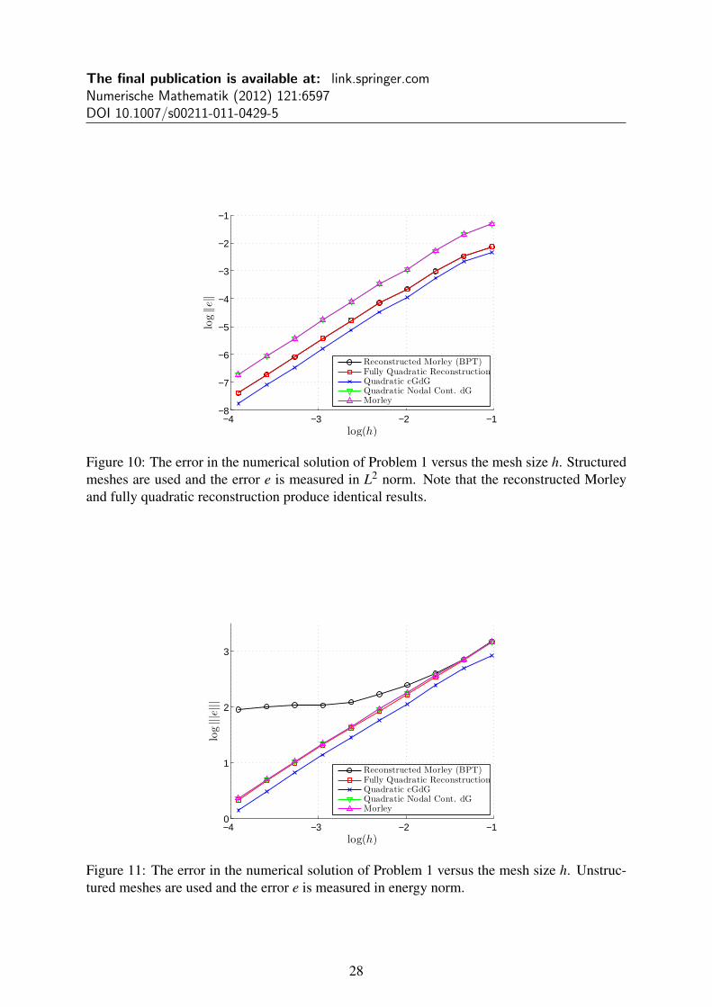
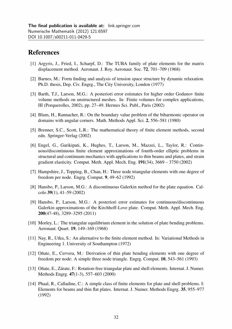
On unstructured meshes the Morley reconstruction/Basic Plate Triangle does not convergeto the analytical solution. This is seen in Figures 11-14. As noted in Remark 4 the Morleyreconstruction does not fulfill the assumption of Theorem 4.6 on unstructured meshes, and thusthe a priori error estimates are not valid. On the other hand, the fully quadratic reconstructiondoes show optimal convergence on unstructured meshes, as predicted by the a priori estimates.In the figures slopes close to 1 for the error in energy norm and slopes close to 2 for the errorin L2 norm indicate optimal convergence. With the noted exception of the Morley reconstruc-tion/Basic Plate Triangle on unstructured meshes, Figures 9-14 indicate optimal convergencefor all the compared methods.

We have previously mentioned that the nonconforming Morley triangle can be seen as aspecial case of the quadratic nodal continuous discontinuous Galerkin method. This is naturalas the β penalty parameter in the dG method enforces continuity of the normal derivativesover each edge midpoint, which is the very definition of the Morley basis functions. As shownin Figures 9-14, the convergence results for the respective method are close to identical forβ = 100 as used in these calculations.

25


https://doi.org/10.1007/s00211-011-0429-5


(a) Collapsed solution due to degenerate patch.

(b) Accurate solution using extended patch.

Figure 7: Numerical solution for a simply supported plate under uniform load using LSFQ-reconstruction including the degenerate patch is shown in (a) and including the extended patchis shown in (b).

26


https://doi.org/10.1007/s00211-011-0429-5


−4 −3 −2 −1−9

−8

−7

−6

−5

−4

−3

−2

−1

log(h)

log‖e

‖

Reconstructed MorleyBasic Plate Triangle

Figure 8: The error in the numerical solution of Problem 1 versus the mesh size h on structuredmeshes. Slopes for the Basic Plate Triangle and the Reconstructed Morley are 1.28 and 1.99respectively. The error e = u−U is measured in L2 norm.

−4 −3 −2 −10

1

2

3

log(h)

log|||

e|||

Reconstructed Morley (BPT)Fully Quadratic ReconstructionQuadratic cGdGQuadratic Nodal Cont. dGMorley

Figure 9: The error in the numerical solution of Problem 1 versus the mesh size h. Structuredmeshes are used and the error e is measured in energy norm. Note that the reconstructed Morleyand fully quadratic reconstruction produce identical results.

27


https://doi.org/10.1007/s00211-011-0429-5


−4 −3 −2 −1−8

−7

−6

−5

−4

−3

−2

−1

log(h)

log‖e

‖


Figure 10: The error in the numerical solution of Problem 1 versus the mesh size h. Structuredmeshes are used and the error e is measured in L2 norm. Note that the reconstructed Morleyand fully quadratic reconstruction produce identical results.

−4 −3 −2 −10

1

2

3

log(h)

log|||

e|||


Figure 11: The error in the numerical solution of Problem 1 versus the mesh size h. Unstruc-tured meshes are used and the error e is measured in energy norm.

28


https://doi.org/10.1007/s00211-011-0429-5


−4 −3 −2 −1−8

−7

−6

−5

−4

−3

−2

−1

log(h)

log‖e

‖


Figure 12: The error in the numerical solution of Problem 1 versus the mesh size h. Unstruc-tured meshes are used and the error e is measured in L2 norm.

−4 −3 −2 −1

−5

−4

−3

−2

log(h)

log|||

e|||


Figure 13: The error in the numerical solution of Problem 2 versus the mesh size h. Unstruc-tured meshes are used and the error e is measured in energy norm.

29


https://doi.org/10.1007/s00211-011-0429-5


−4 −3 −2 −1−12

−11

−10

−9

−8

−7

−6

−5

−4

log(h)

log‖e

‖


Figure 14: The error in the numerical solution of Problem 2 versus the mesh size h. Unstruc-tured meshes are used and the error e is measured in L2 norm.

5.4.3 Number of Degrees of Freedom

To give some indication of the performance of these elements in regards to how many degreesof freedom are needed to represent the solution we give Figure 15. While it is seen in Figures9-14 that the quadratic cG/dG method has the best performance among the tested methods withrespect to mesh discretization, Figure 15 indicates that the fully quadratic reconstruction has themost compact representation performance wise. This is natural as we have smooth solutions.Even though the quadratic nodal continuous dG method produce results close to identical tothose of the Morley triangle with regards to mesh discretization it does feature two degrees offreedom on each edge midpoint compared to one for the Morley triangle, explaining that moredegrees of freedom are needed for par performance.

5.4.4 Size of penalty parameter β

In Figure 16 we present some numerical results for various β . As might be suspected thefully quadratic reconstruction exhibits locking effects when β is to large. This is natural asneighbouring elements share much of the information through the patch construction. A moresurprising result is that the quadratic cG/dG method does not seem to exhibit such locking ef-fects for large β . This indicates that the finite element space of continuous piecewise quadraticpolynomials with continuous normal gradients on edge midpoints is large enough to accuratelyapproximate the solution. If we on the other hand change the projection operator in the penaltyterm from the projection onto constants P0 to the projection onto linear functions P1 the cG/dGmethod exhibits locking effects for large β .

A mesh independent lower bound for β can be calculated if a suitable choice of h in (2.30)on each edge is made, see [9]. However, for the numerical results in this paper we have used aglobal mesh size parameter for h. As the meshes used in the numerical results in this paper arequasi-uniform this should be sufficient.

30


https://doi.org/10.1007/s00211-011-0429-5


3 4 5 6 7 8 9 10 11

−5

−4

−3

−2

log(dofs)

log|||

e|||


Figure 15: The error in the numerical solution of Problem 2 versus the number of degrees offreedom needed. Unstructured meshes are used and the error e is measured in energy norm.

−4 −3 −2 −1−1

0

1

2

3

4

log(h)

log|||

e|||

Fully Quadratic ReconstructionQuadratic cGdG P0

Quadratic cGdG P1

Figure 16: The error in the numerical solution of Problem 1 versus the mesh size using variousβ . Solid lines indicate β = 102, dashed lines indicate β = 104, and dash-dot lines indicateβ = 106. Unstructured meshes are used and the error e is measured in energy norm.

31


https://doi.org/10.1007/s00211-011-0429-5


References[1] Argyris, J., Fried, I., Scharpf, D.: The TUBA family of plate elements for the matrix

displacement method. Aeronaut. J. Roy. Aeronaut. Soc. 72, 701–709 (1968)

[2] Barnes, M.: Form finding and analysis of tension space structure by dynamic relaxation.Ph.D. thesis, Dep. Civ. Engrg., The City University, London (1977)

[3] Barth, T.J., Larson, M.G.: A posteriori error estimates for higher order Godunov finitevolume methods on unstructured meshes. In: Finite volumes for complex applications,III (Porquerolles, 2002), pp. 27–49. Hermes Sci. Publ., Paris (2002)

[4] Blum, H., Rannacher, R.: On the boundary value problem of the biharmonic operator ondomains with angular corners. Math. Methods Appl. Sci. 2, 556–581 (1980)

[5] Brenner, S.C., Scott, L.R.: The mathematical theory of finite element methods, secondedn. Springer-Verlag (2002)

[6] Engel, G., Garikipati, K., Hughes, T., Larson, M., Mazzei, L., Taylor, R.: Contin-uous/discontinuous finite element approximations of fourth-order elliptic problems instructural and continuum mechanics with applications to thin beams and plates, and straingradient elasticity. Comput. Meth. Appl. Mech. Eng. 191(34), 3669 – 3750 (2002)

[7] Hampshire, J., Topping, B., Chan, H.: Three node triangular elements with one degree offreedom per node. Engrg. Comput. 9, 49–62 (1992)

[8] Hansbo, P., Larson, M.G.: A discontinuous Galerkin method for the plate equation. Cal-colo 39(1), 41–59 (2002)

[9] Hansbo, P., Larson, M.G.: A posteriori error estimates for continuous/discontinuousGalerkin approximations of the Kirchhoff-Love plate. Comput. Meth. Appl. Mech. Eng.200(47-48), 3289–3295 (2011)

[10] Morley, L.: The triangular equilibrium element in the solution of plate bending problems.Aeronaut. Quart. 19, 149–169 (1968)

[11] Nay, R., Utku, S.: An alternative to the finite element method. In: Variational Methods inEngineering 1. University of Southampton (1972)

[12] Onate, E., Cervera, M.: Derivation of thin plate bending elements with one degree offreedom per node: A simple three node triangle. Engrg. Comput. 10, 543–561 (1993)

[13] Onate, E., Zarate, F.: Rotation-free triangular plate and shell elements. Internat. J. Numer.Methods Engrg. 47(1-3), 557–603 (2000)

[14] Phaal, R., Calladine, C.: A simple class of finite elements for plate and shell problems. I:Elements for beams and thin flat plates. Internat. J. Numer. Methods Engrg. 35, 955–977(1992)

32


https://doi.org/10.1007/s00211-011-0429-5


[15] Phaal, R., Calladine, C.: A simple class of finite elements for plate and shell problems. II:An element for thin shells, with only translational degrees of freedom. Internat. J. Numer.Methods Engrg. 35, 979–996 (1992)

[16] Timoshenko, S., Woinowsky-Krieger, S.: Theory of plates and shells, second edn.McGraw-Hill (1959)

33


https://doi.org/10.1007/s00211-011-0429-5

Continuous Piecewise Linear Finite Elements for the ... · PDF fileKirchhoff–Love Plate...

Documents

Transcript of Continuous Piecewise Linear Finite Elements for the ... · PDF fileKirchhoff–Love Plate...