Contingency Tables - University of Washington

Summer 2017 Summer Institutes

Contingency Tables

187


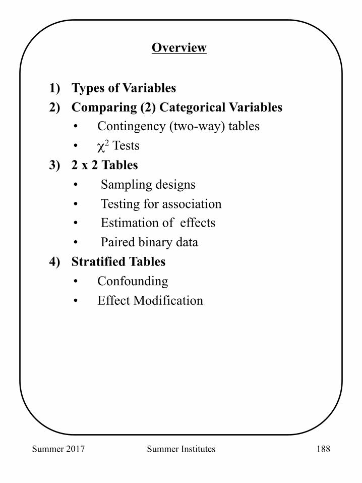
Overview

1)   Types of Variables 2)   Comparing (2) Categorical Variables

•  Contingency (two-way) tables •  χ2 Tests

3)   2 x 2 Tables •  Sampling designs •  Testing for association •  Estimation of effects •  Paired binary data

4)   Stratified Tables •  Confounding •  Effect Modification

188


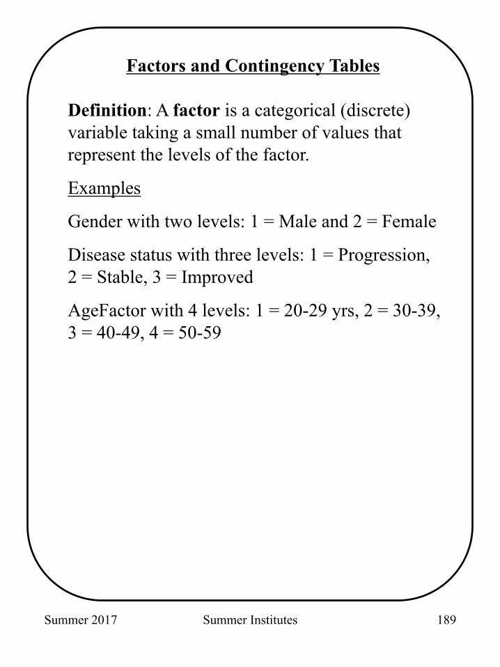
Factors and Contingency Tables

Definition: A factor is a categorical (discrete) variable taking a small number of values that represent the levels of the factor.

Examples

Gender with two levels: 1 = Male and 2 = Female

Disease status with three levels: 1 = Progression, 2 = Stable, 3 = Improved

AgeFactor with 4 levels: 1 = 20-29 yrs, 2 = 30-39, 3 = 40-49, 4 = 50-59

189


Factors and Contingency Tables

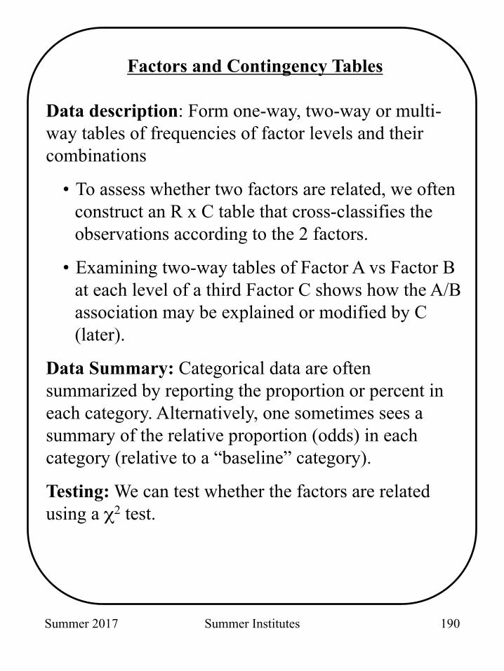
Data description: Form one-way, two-way or multi-way tables of frequencies of factor levels and their combinations

•  To assess whether two factors are related, we often construct an R x C table that cross-classifies the observations according to the 2 factors.

•  Examining two-way tables of Factor A vs Factor B at each level of a third Factor C shows how the A/B association may be explained or modified by C (later).

Data Summary: Categorical data are often summarized by reporting the proportion or percent in each category. Alternatively, one sometimes sees a summary of the relative proportion (odds) in each category (relative to a “baseline” category).

Testing: We can test whether the factors are related using a χ2 test.

190


Categorical Data

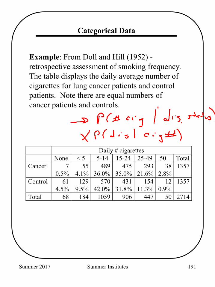
Example: From Doll and Hill (1952) - retrospective assessment of smoking frequency. The table displays the daily average number of cigarettes for lung cancer patients and control patients. Note there are equal numbers of cancer patients and controls.

Daily # cigarettes None < 5 5-14 15-24 25-49 50+ Total Cancer 7

0.5% 55

4.1% 489

36.0% 475

35.0% 293

21.6% 38

2.8% 1357

Control 61 4.5%

129 9.5%

570 42.0%

431 31.8%

154 11.3%

12 0.9%

1357

Total 68 184 1059 906 447 50 2714

191


χ2 Test

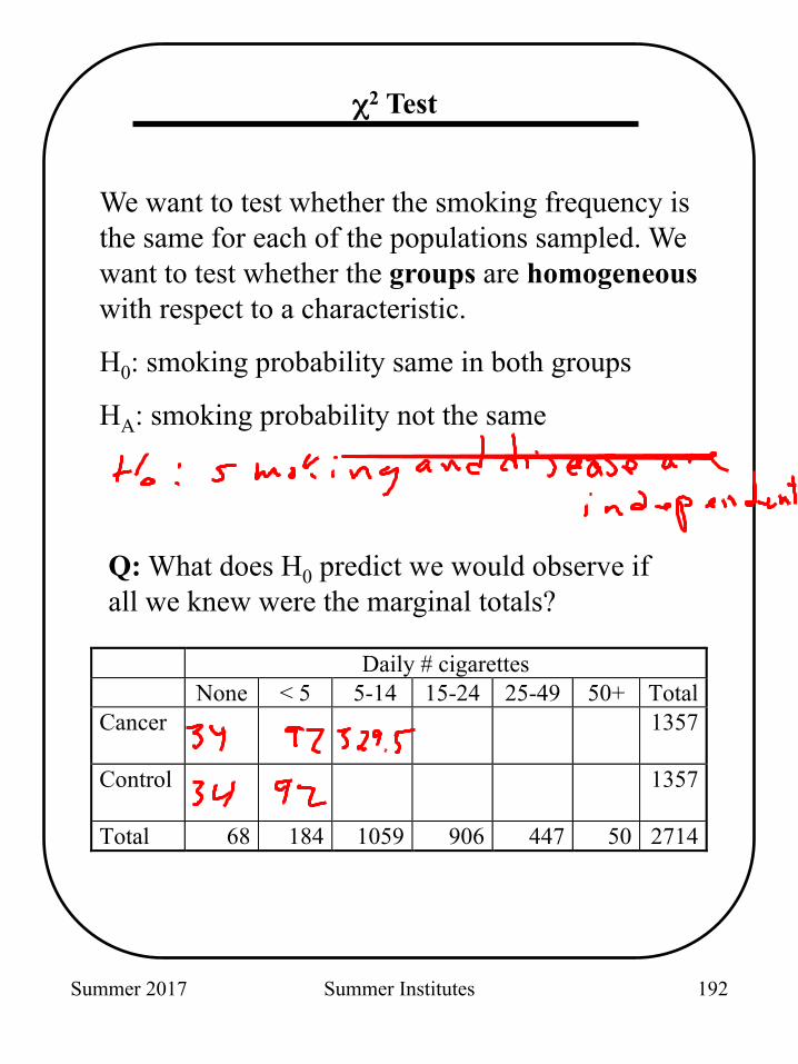
We want to test whether the smoking frequency is the same for each of the populations sampled. We want to test whether the groups are homogeneous with respect to a characteristic.

H0: smoking probability same in both groups

HA: smoking probability not the same

Q: What does H0 predict we would observe if all we knew were the marginal totals?

Daily # cigarettes None < 5 5-14 15-24 25-49 50+ Total Cancer

1357

Control

1357

Total 68 184 1059 906 447 50 2714

192


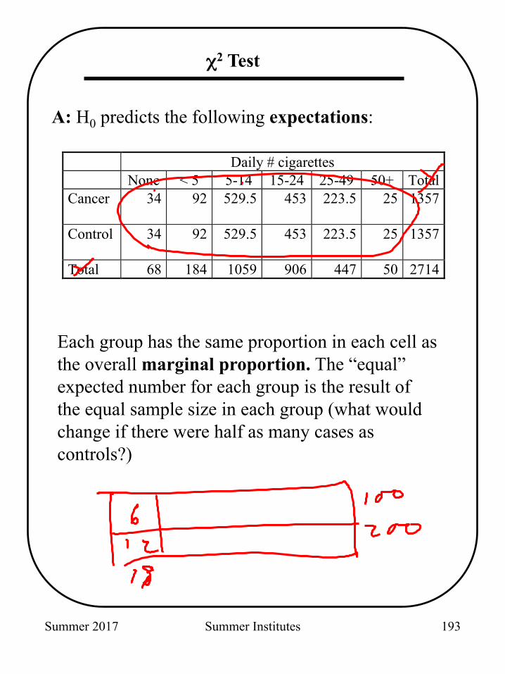
Daily # cigarettes None < 5 5-14 15-24 25-49 50+ Total Cancer 34 92 529.5 453 223.5 25

1357

Control 34 92 529.5 453 223.5 25

1357

Total 68 184 1059 906 447 50 2714

A: H0 predicts the following expectations:

Each group has the same proportion in each cell as the overall marginal proportion. The “equal” expected number for each group is the result of the equal sample size in each group (what would change if there were half as many cases as controls?)

χ2 Test

193


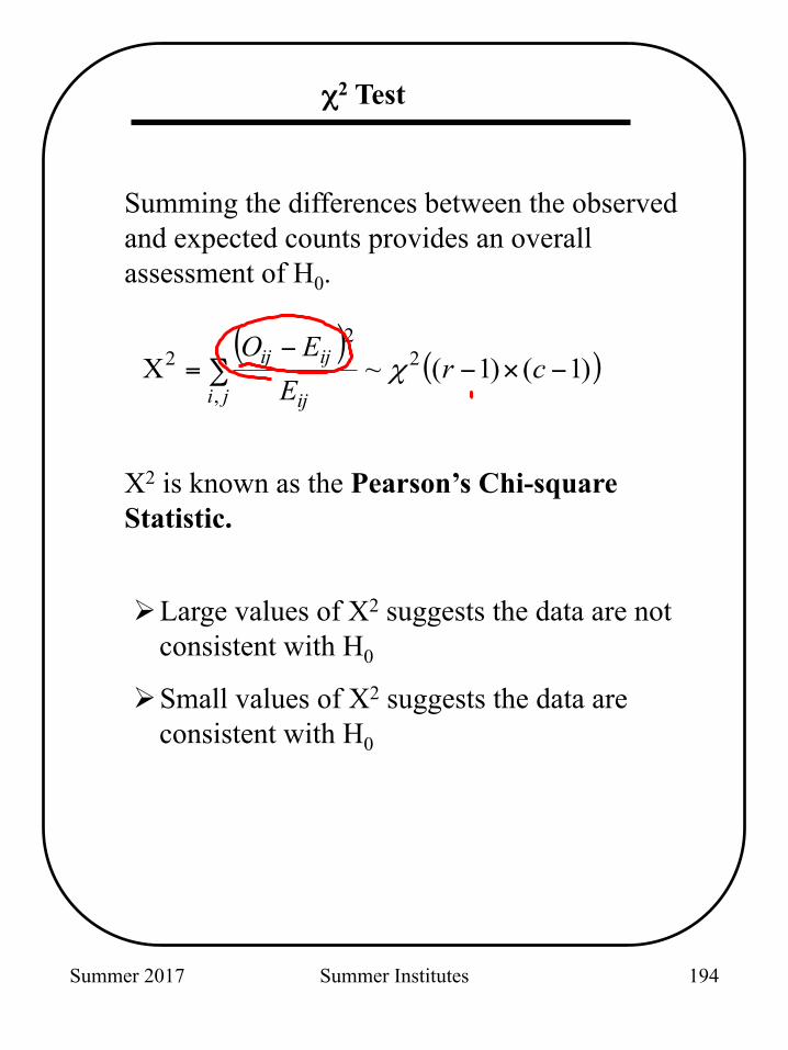
Summing the differences between the observed and expected counts provides an overall assessment of H0.

X2 is known as the Pearson’s Chi-square Statistic.

( )( ))1()1(~X 2

,

22 −×−∑

−= cr

EEO

ji ij

ijij χ

Ø Large values of X2 suggests the data are not consistent with H0

Ø Small values of X2 suggests the data are consistent with H0

χ2 Test

194


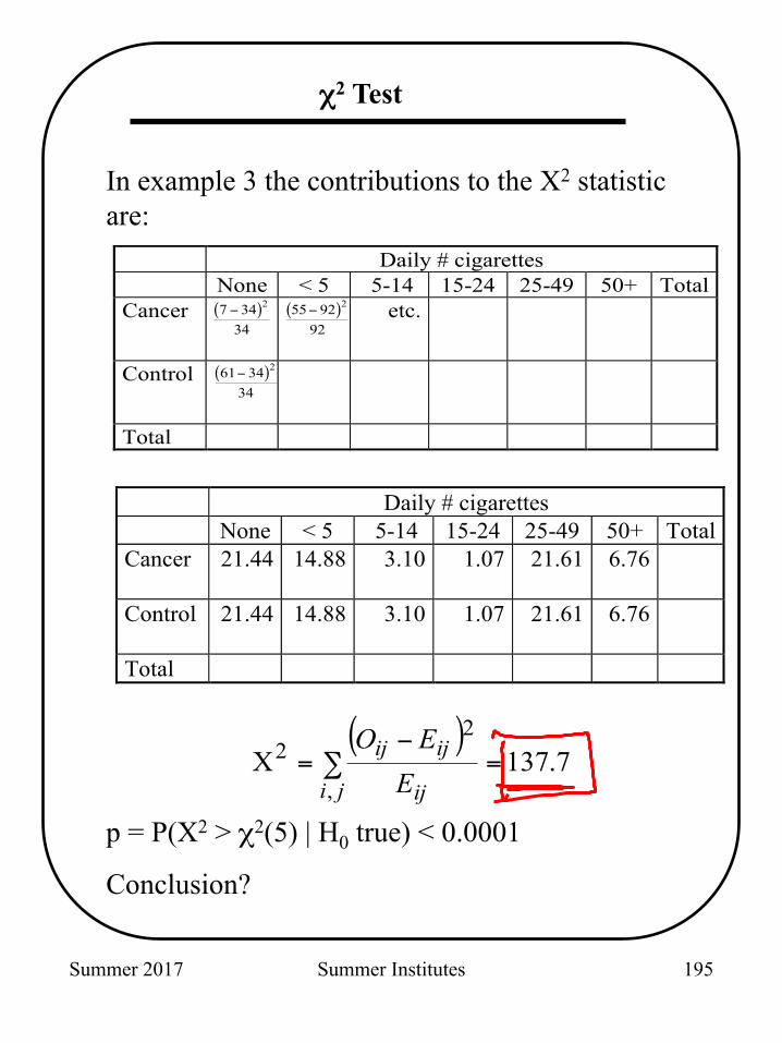
In example 3 the contributions to the X2 statistic are:

Daily # cigarettes None < 5 5-14 15-24 25-49 50+ Total Cancer ( )7 34

34

2−

( )55 9292

2−

etc.

Control ( )61 3434

2−

Total

Daily # cigarettes None < 5 5-14 15-24 25-49 50+ Total Cancer 21.44 14.88 3.10 1.07 21.61 6.76

Control 21.44 14.88 3.10 1.07 21.61 6.76

Total

( )7.137X

,

22 =∑

−=

ji ij

ijij

EEO

p = P(X2 > χ2(5) | H0 true) < 0.0001

Conclusion?

χ2 Test

195


Factor Levels 1 2 … C Total

1 O11 O12 … O1C N1 Group

2 O21 N2

3 O31 N3

! ! R OR1 ORC NR

Total M1 M2 MC T

1.  Compute the expected cell counts under homogeneity assumption:

Eij = NiMj/T

2.  Compute the chi-square statistic:

3.  Compare X2 to χ2(df) where

df = (R-1) x (C-1)

4.  Interpret acceptance/rejection or p-value.

( )∑

−=

ji ij

ijij

EEO

,

22X

χ2 Test

196


2 x 2 Tables

Example 1: Pauling (1971)

Patients are randomized to either receive Vitamin C or placebo. Patients are followed-up to ascertain the development of a cold.

Q: Is treatment with Vitamin C associated with a reduced probability of getting a cold?

Q: If Vitamin C is associated with reducing colds, then what is the magnitude of the effect?

Cold - Y Cold - N Total Vitamin C 17 122 139

Placebo 31 109 140

Total 48 231 279

197


2 x 2 Tables

Example 2: Keller (AJPH, 1965)

Patients with (cases) and without (controls) oral cancer were surveyed regarding their smoking frequency (this table collapses over the smoking frequency categories).

Q: Is oral cancer associated with smoking?

Q: If smoking is associated with oral cancer, then what is the magnitude of the risk?

Case Control TotalSmoker 484 385 869

Non-Smoker

27 90 117

Total 511 475 986

198


2 x 2 Tables

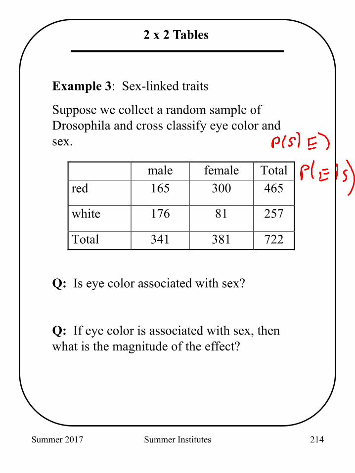
Example 3: Sex-linked traits

Suppose we collect a random sample of Drosophila and cross classify eye color and sex.

Q: Is eye color associated with sex?

Q: If eye color is associated with sex, then what is the magnitude of the effect?

male female Total red 165 300 465

white 176 81 257

Total 341 381 722

199


2 x 2 Tables

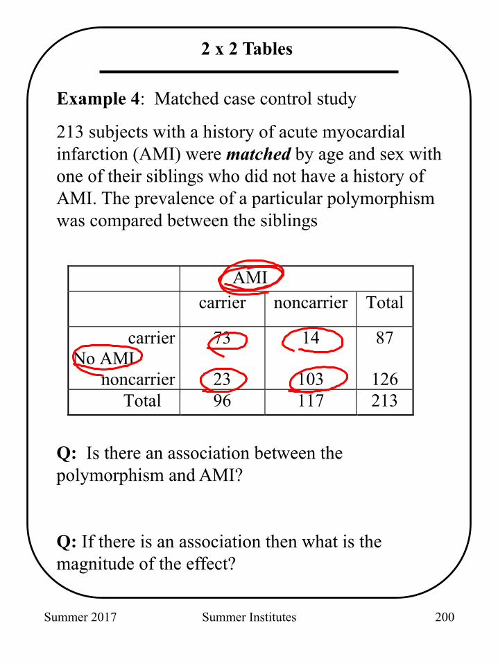
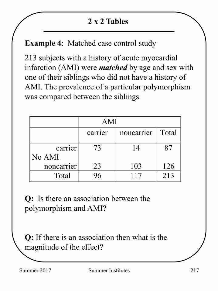
Example 4: Matched case control study

213 subjects with a history of acute myocardial infarction (AMI) were matched by age and sex with one of their siblings who did not have a history of AMI. The prevalence of a particular polymorphism was compared between the siblings

Q: Is there an association between the polymorphism and AMI?

Q: If there is an association then what is the magnitude of the effect?

AMI carrier noncarrier Total

carrier No AMI

noncarrier

73

23

14

103

87

126 Total 96 117 213

200


2 x 2 Tables

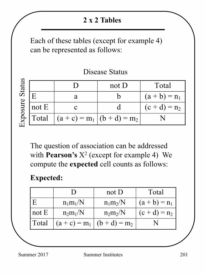
Each of these tables (except for example 4) can be represented as follows:

The question of association can be addressed with Pearson’s X2 (except for example 4) We compute the expected cell counts as follows:

Expected:

D not D Total E a b (a + b) = n1

not E c d (c + d) = n2

Total (a + c) = m1 (b + d) = m2 N

D not D Total E n1m1/N n1m2/N (a + b) = n1

not E n2m1/N n2m2/N (c + d) = n2

Total (a + c) = m1 (b + d) = m2 N

Disease Status

Expo

sure

Sta

tus

201


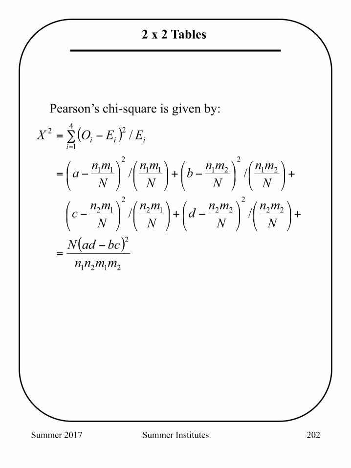
Pearson’s chi-square is given by:

2 x 2 Tables

( )

( )2121

2

222

22122

12

212

21112

11

4

1

22

//

//

/

mmnnbcadN

Nmn

Nmnd

Nmn

Nmnc

Nmn

Nmnb

Nmn

Nmna

EEOXi

iii

−=

+⎟⎠⎞

⎜⎝⎛

⎟⎠⎞

⎜⎝⎛ −+⎟

⎠⎞

⎜⎝⎛

⎟⎠⎞

⎜⎝⎛ −

+⎟⎠⎞

⎜⎝⎛

⎟⎠⎞

⎜⎝⎛ −+⎟

⎠⎞

⎜⎝⎛

⎟⎠⎞

⎜⎝⎛ −=

∑ −==

202


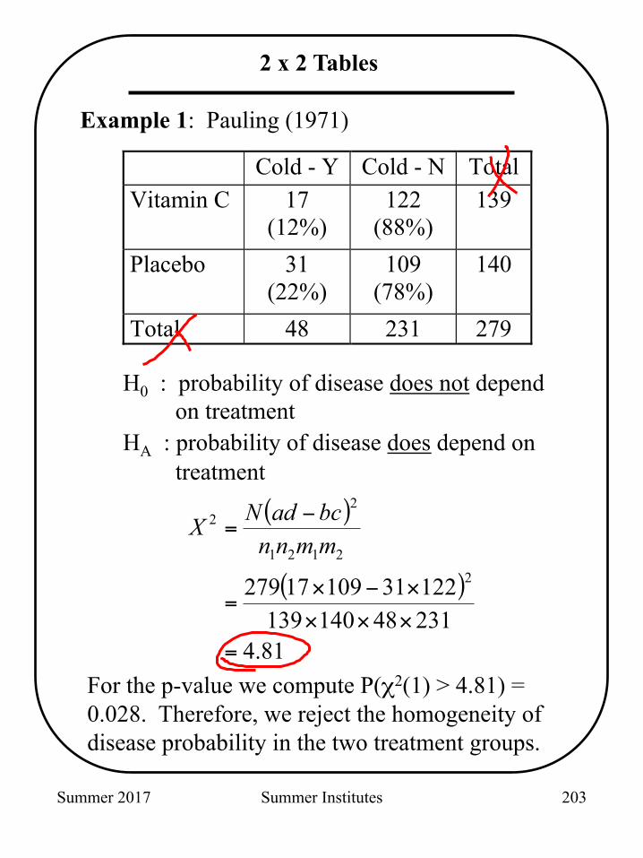
Example 1: Pauling (1971)

H0 : probability of disease does not depend

on treatment HA : probability of disease does depend on

treatment

2 x 2 Tables

( )

( )

81.4231481401391223110917279 2

2121

22

=××××−×

=

−=

mmnnbcadNX

For the p-value we compute P(χ2(1) > 4.81) = 0.028. Therefore, we reject the homogeneity of disease probability in the two treatment groups.

Cold - Y Cold - N Total Vitamin C 17

(12%) 122

(88%) 139

Placebo 31 (22%)

109 (78%)

140

Total 48 231 279

203


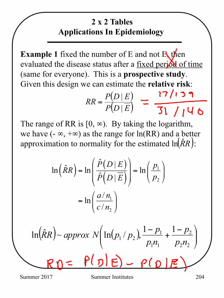
Example 1 fixed the number of E and not E, then evaluated the disease status after a fixed period of time (same for everyone). This is a prospective study. Given this design we can estimate the relative risk: The range of RR is [0, ∞). By taking the logarithm, we have (- ∞, +∞) as the range for ln(RR) and a better approximation to normality for the estimated ln

( ):ˆRR

2 x 2 Tables Applications In Epidemiology

( )( )EDP

EDPRR||

=

( ) ( )( )

1

2

1

2

ˆ |ˆln ln lnˆ |

/ln/

P D E pRRpP D E

a nc n

⎛ ⎞ ⎛ ⎞⎜ ⎟= = ⎜ ⎟⎜ ⎟ ⎝ ⎠⎝ ⎠

⎛ ⎞= ⎜ ⎟

⎝ ⎠

( ) ( ) ⎟⎟⎠

⎞⎜⎜⎝

⎛ −+

−

22

2

11

121

11 ,/ln~ˆlnnpp

nppppNapproxRR

204


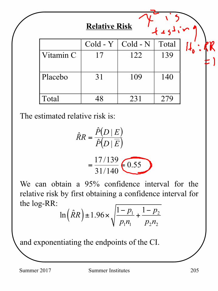
The estimated relative risk is:

We can obtain a 95% confidence interval for the relative risk by first obtaining a confidence interval for the log-RR:

( )( )

55.0140/31139/17

|ˆ|ˆˆ

==

=EDPEDPRR

( ) 1 2

1 1 2 2

1 1ˆln 1.96 p pRRp n p n− −

± × +

Cold - Y Cold - N Total Vitamin C 17 122 139

Placebo 31 109 140

Total 48 231 279

Relative Risk

and exponentiating the endpoints of the CI.

205


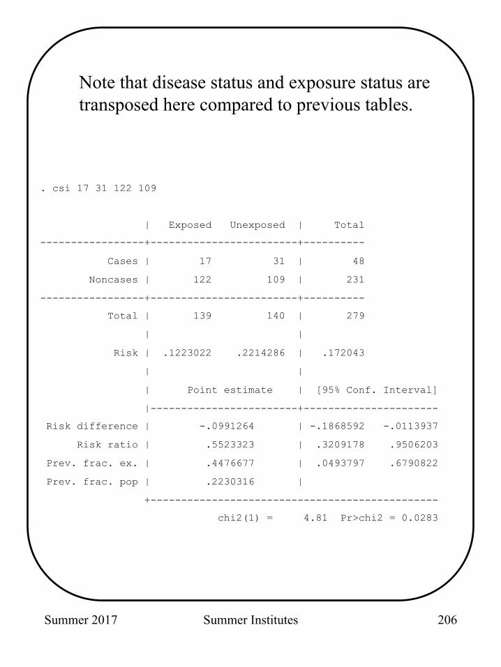
. csi 17 31 122 109

| Exposed Unexposed | Total

-----------------+------------------------+----------

Cases | 17 31 | 48

Noncases | 122 109 | 231

-----------------+------------------------+----------

Total | 139 140 | 279

| |

Risk | .1223022 .2214286 | .172043

| |

| Point estimate | [95% Conf. Interval]

|------------------------+----------------------

Risk difference | -.0991264 | -.1868592 -.0113937

Risk ratio | .5523323 | .3209178 .9506203

Prev. frac. ex. | .4476677 | .0493797 .6790822

Prev. frac. pop | .2230316 |

+-----------------------------------------------

chi2(1) = 4.81 Pr>chi2 = 0.0283

Note that disease status and exposure status are transposed here compared to previous tables.

206


2 x 2 Tables

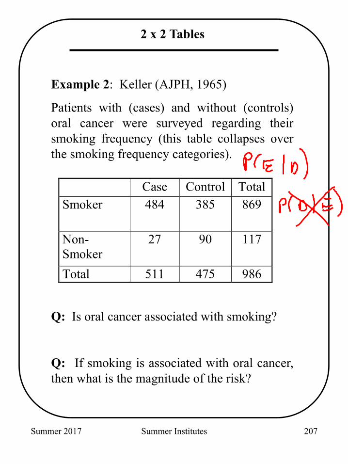
Example 2: Keller (AJPH, 1965)

Patients with (cases) and without (controls) oral cancer were surveyed regarding their smoking frequency (this table collapses over the smoking frequency categories).

Q: Is oral cancer associated with smoking?

Q: If smoking is associated with oral cancer, then what is the magnitude of the risk?

Case Control TotalSmoker 484 385 869

Non-Smoker

27 90 117

Total 511 475 986

207


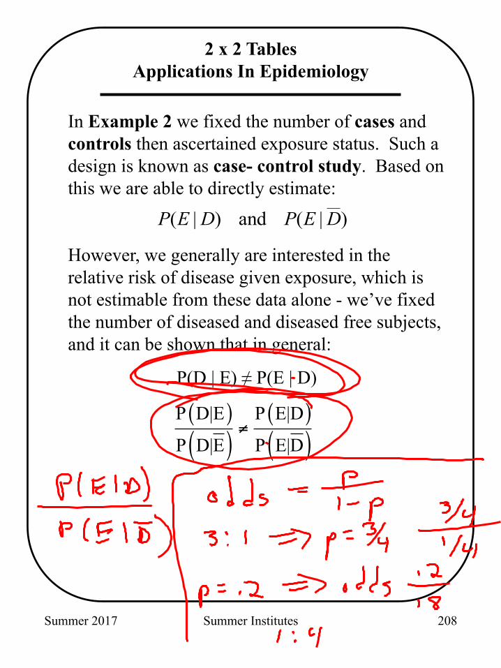
2 x 2 Tables Applications In Epidemiology

In Example 2 we fixed the number of cases and controls then ascertained exposure status. Such a design is known as case- control study. Based on this we are able to directly estimate:

However, we generally are interested in the relative risk of disease given exposure, which is not estimable from these data alone - we’ve fixed the number of diseased and diseased free subjects, and it can be shown that in general:

P(D | E) ≠ P(E | D)

)|(and)|( DEPDEP

( )( )

( )( )

P D|E P E|D

P D|E P E|D≠

208


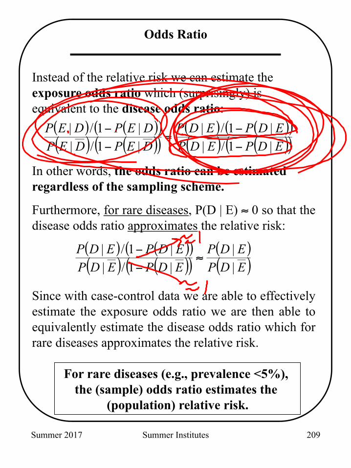
Odds Ratio

Instead of the relative risk we can estimate the exposure odds ratio which (surprisingly) is equivalent to the disease odds ratio: In other words, the odds ratio can be estimated regardless of the sampling scheme.

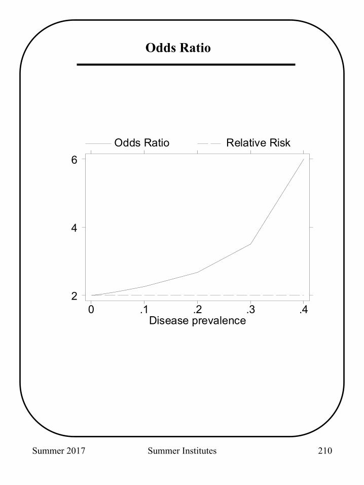
Furthermore, for rare diseases, P(D | E) ≈ 0 so that the disease odds ratio approximates the relative risk:

Since with case-control data we are able to effectively estimate the exposure odds ratio we are then able to equivalently estimate the disease odds ratio which for rare diseases approximates the relative risk.

( ) ( )( )( ) ( )( )

( )( )EDP

EDPEDPEDPEDPEDP

||

|1/||1/|

≈−−

For rare diseases (e.g., prevalence <5%), the (sample) odds ratio estimates the

(population) relative risk.

( ) ( )( )( ) ( )( )

( ) ( )( )( ) ( )( )EDPEDP

EDPEDPDEPDEPDEPDEP

|1/||1/|

|1/||1/|

−−

=−−

209


Disease prevalence

Odds Ratio Relative Risk

0 .1 .2 .3 .42

4

6

Odds Ratio

210


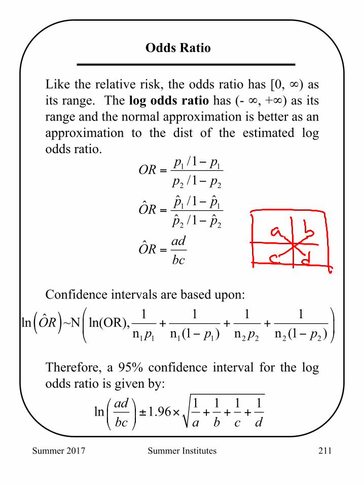
Like the relative risk, the odds ratio has [0, ∞) as its range. The log odds ratio has (- ∞, +∞) as its range and the normal approximation is better as an approximation to the dist of the estimated log odds ratio.

Confidence intervals are based upon:

Therefore, a 95% confidence interval for the log odds ratio is given by:

Odds Ratio

1 1

2 2

1 1

2 2

/1/1

ˆ ˆ/1ˆˆ ˆ/1

ˆ

p pORp pp pORp padORbc

−=

−

−=

−

=

( )1 1 1 1 2 2 2 2

1 1 1 1ˆln ~N ln(OR),n n (1 ) n n (1 )

ORp p p p

⎛ ⎞+ + +⎜ ⎟− −⎝ ⎠

1 1 1 1ln 1.96adbc a b c d

⎛ ⎞ ± × + + +⎜ ⎟⎝ ⎠

211


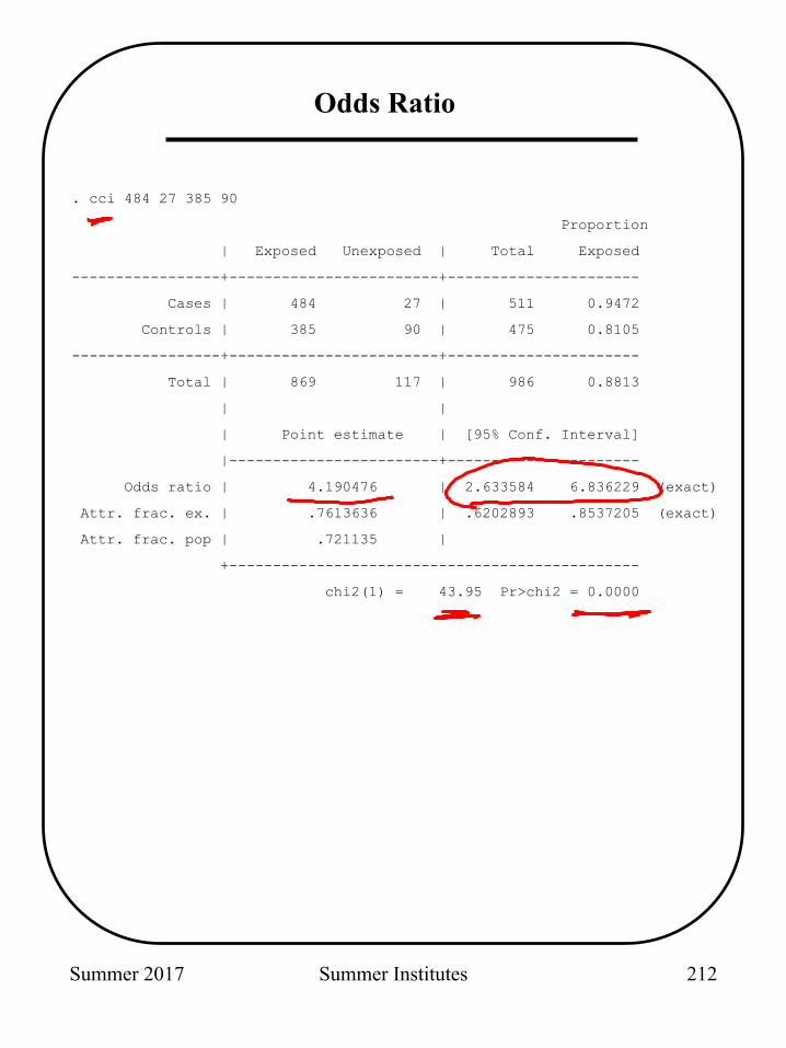
. cci 484 27 385 90

Proportion

| Exposed Unexposed | Total Exposed

-----------------+------------------------+----------------------

Cases | 484 27 | 511 0.9472

Controls | 385 90 | 475 0.8105

-----------------+------------------------+----------------------

Total | 869 117 | 986 0.8813

| |


|------------------------+----------------------

Odds ratio | 4.190476 | 2.633584 6.836229 (exact)

Attr. frac. ex. | .7613636 | .6202893 .8537205 (exact)

Attr. frac. pop | .721135 |

+-----------------------------------------------

chi2(1) = 43.95 Pr>chi2 = 0.0000

Odds Ratio

212


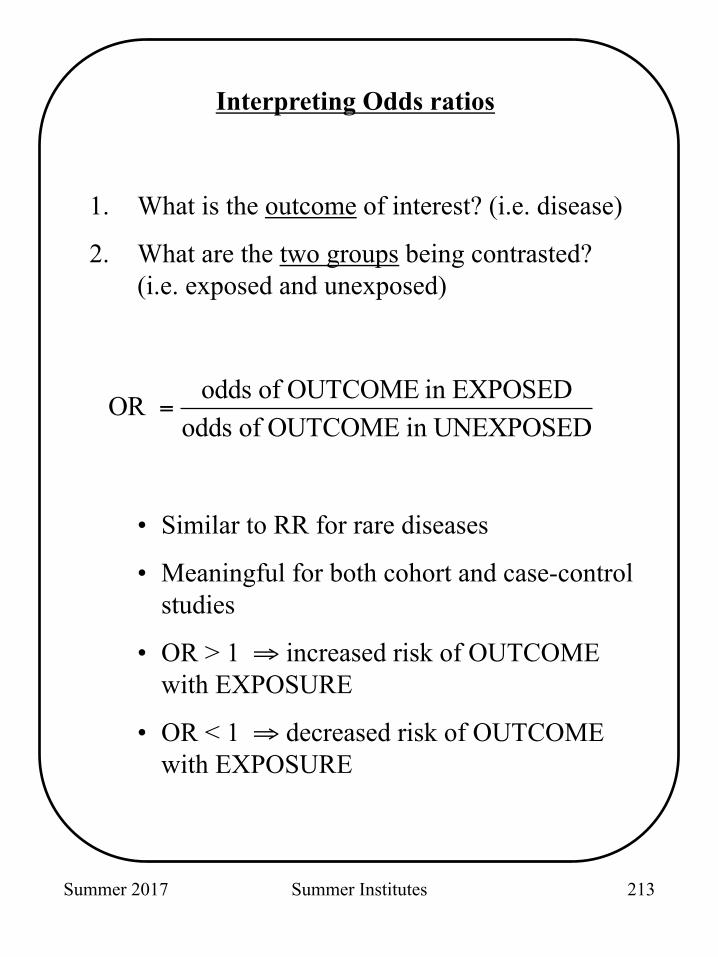
Interpreting Odds ratios

1.  What is the outcome of interest? (i.e. disease)

2.  What are the two groups being contrasted? (i.e. exposed and unexposed)

odds of OUTCOME in EXPOSEDOR odds of OUTCOME in UNEXPOSED

=

•  Similar to RR for rare diseases

•  Meaningful for both cohort and case-control studies

•  OR > 1 ⇒ increased risk of OUTCOME with EXPOSURE

•  OR < 1 ⇒ decreased risk of OUTCOME with EXPOSURE

213


2 x 2 Tables

Example 3: Sex-linked traits

Suppose we collect a random sample of Drosophila and cross classify eye color and sex.

Q: Is eye color associated with sex?

Q: If eye color is associated with sex, then what is the magnitude of the effect?

male female Total red 165 300 465

white 176 81 257

Total 341 381 722

214


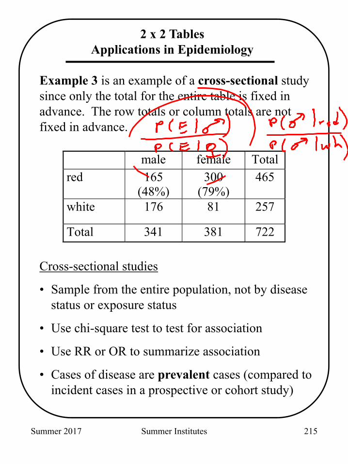
2 x 2 Tables Applications in Epidemiology

Example 3 is an example of a cross-sectional study since only the total for the entire table is fixed in advance. The row totals or column totals are not fixed in advance.

Cross-sectional studies

•  Sample from the entire population, not by disease status or exposure status

•  Use chi-square test to test for association

•  Use RR or OR to summarize association

•  Cases of disease are prevalent cases (compared to incident cases in a prospective or cohort study)

male female Total red 165

(48%) 300

(79%) 465

white 176 81 257

Total 341 381 722

215


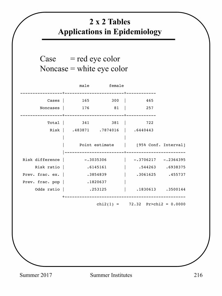
male female

-----------------+------------------------+------------

Cases | 165 300 | 465

Noncases | 176 81 | 257

-----------------+------------------------+------------

Total | 341 381 | 722

Risk | .483871 .7874016 | .6440443

| |


|------------------------+------------------------

Risk difference | -.3035306 | -.3706217 -.2364395

Risk ratio | .6145161 | .544263 .6938375

Prev. frac. ex. | .3854839 | .3061625 .455737

Prev. frac. pop | .1820637 |

Odds ratio | .253125 | .1830613 .3500144

+-------------------------------------------------

chi2(1) = 72.32 Pr>chi2 = 0.0000

2 x 2 Tables Applications in Epidemiology

Case = red eye color Noncase = white eye color

216


2 x 2 Tables

Example 4: Matched case control study

213 subjects with a history of acute myocardial infarction (AMI) were matched by age and sex with one of their siblings who did not have a history of AMI. The prevalence of a particular polymorphism was compared between the siblings

Q: Is there an association between the polymorphism and AMI?

Q: If there is an association then what is the magnitude of the effect?


carrier No AMI

noncarrier

73

23

14

103

87

126 Total 96 117 213

217


Paired Binary Data

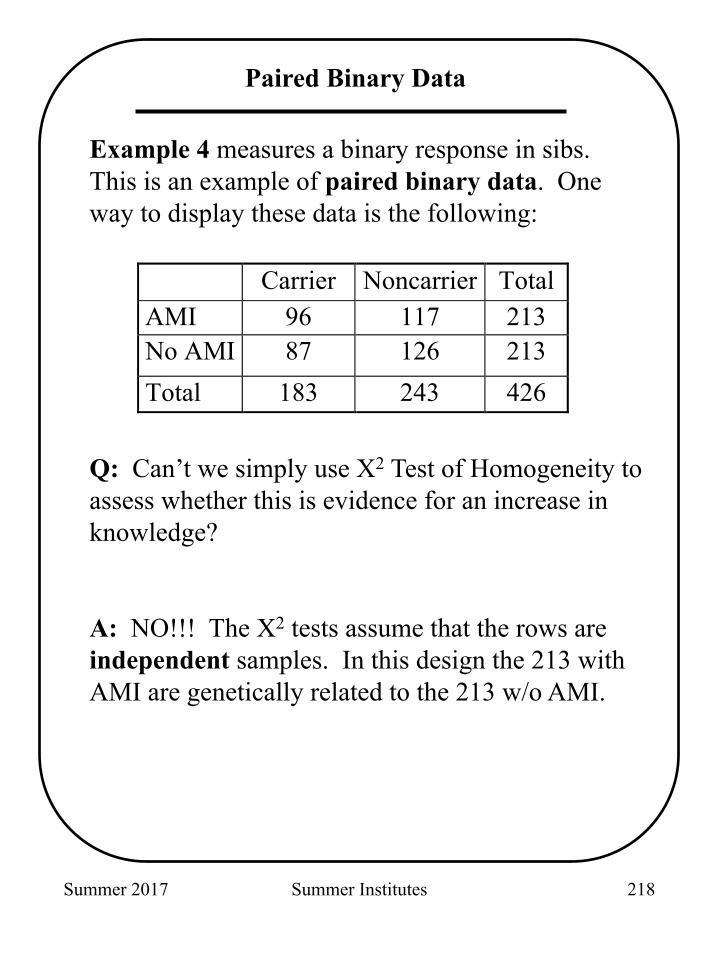
Example 4 measures a binary response in sibs. This is an example of paired binary data. One way to display these data is the following:

Q: Can’t we simply use X2 Test of Homogeneity to assess whether this is evidence for an increase in knowledge?

A: NO!!! The X2 tests assume that the rows are independent samples. In this design the 213 with AMI are genetically related to the 213 w/o AMI.

Carrier Noncarrier Total AMI 96 117 213 No AMI 87 126 213 Total 183 243 426

218


Paired Binary Data

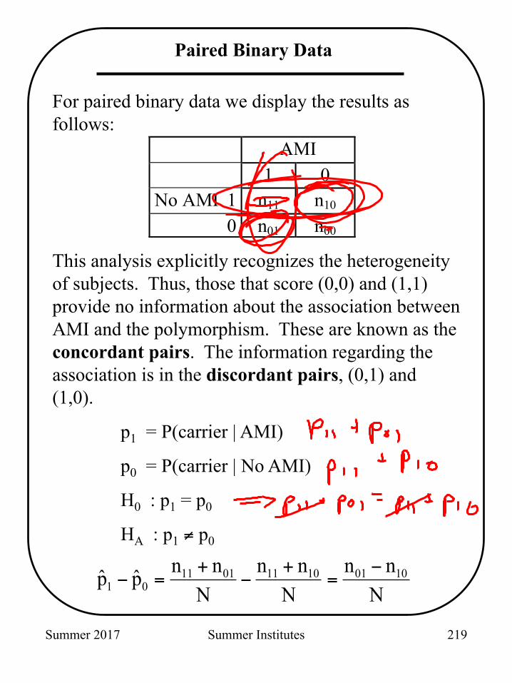
For paired binary data we display the results as follows:

This analysis explicitly recognizes the heterogeneity of subjects. Thus, those that score (0,0) and (1,1) provide no information about the association between AMI and the polymorphism. These are known as the concordant pairs. The information regarding the association is in the discordant pairs, (0,1) and (1,0).

p1 = P(carrier | AMI)

p0 = P(carrier | No AMI)

H0 : p1 = p0

HA : p1 ≠ p0

AMI 1 0 No AMI 1 n11 n10

0 n01 n00

Nnn

Nnn

Nnnp̂ p̂ 100110110111

01−

=+

−+

=−

219


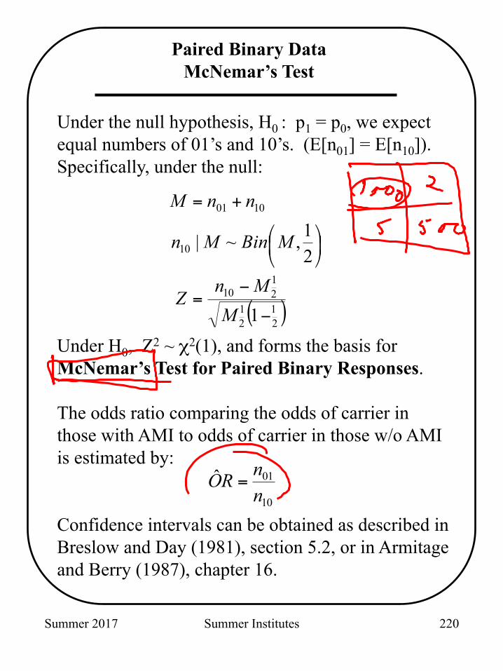
Under the null hypothesis, H0 : p1 = p0, we expect equal numbers of 01’s and 10’s. (E[n01] = E[n10]). Specifically, under the null: Under H0, Z2 ~ χ2(1), and forms the basis for McNemar’s Test for Paired Binary Responses. The odds ratio comparing the odds of carrier in those with AMI to odds of carrier in those w/o AMI is estimated by: Confidence intervals can be obtained as described in Breslow and Day (1981), section 5.2, or in Armitage and Berry (1987), chapter 16.

Paired Binary Data McNemar’s Test

( )1212

1210

10

1001

1

21,~|

−

−=

⎟⎠⎞

⎜⎝⎛

+=

MMn

Z

MBinMn

nnM

10

01ˆnnRO =

220


Example 4:

We can test H0: p1 = p2 using McNemar’s Test:

Comparing 1.482 to a χ2 (1) we find that p > 0.05. Therefore, we do not reject the null hypothesis and find little evidence of association between gene and disease.

We estimate the odds ratio as

( )( )

( )

101 2

1 12 2

23 23 14 / 2

23 14 / 4

1.48

n MZ

M

−=

− +=

+

=

ˆ 23/14 1.64.OR = =


carrier No AMI

noncarrier

73

23

14

103

87

126 Total 96 117 213

221


Matched case-control data

. mcci 73 23 14 103 | Controls | Cases | Exposed Unexposed | Total -----------------+------------------------+------------ Exposed | 73 23 | 96 Unexposed | 14 103 | 117 -----------------+------------------------+------------ Total | 87 126 | 213 McNemar's chi2(1) = 2.19 Prob > chi2 = 0.1390 Exact McNemar significance probability = 0.1877 Proportion with factor Cases .4507042 Controls .4084507 [95% Conf. Interval] --------- -------------------- difference .0422535 -.0181247 .1026318 ratio 1.103448 .9684942 1.257207 rel. diff. .0714286 -.0197486 .1626057 odds ratio 1.642857 .8101776 3.452833 (exact)

222


Two way tables - Review

• How were data collected? • Cohort design • Case-control design • Cross-sectional design • Matched pairs

•  Is there an association? •  R x C Tables

• Chi-square tests of Homogeneity & Independence

•  2 x 2 Tables • Chi-square test •  Paired data and McNemar's

• What is the magnitude of the association? • Relative risk • Odds ratio (≈ relative risk for rare diseases) • Risk difference (attributable risk)

223


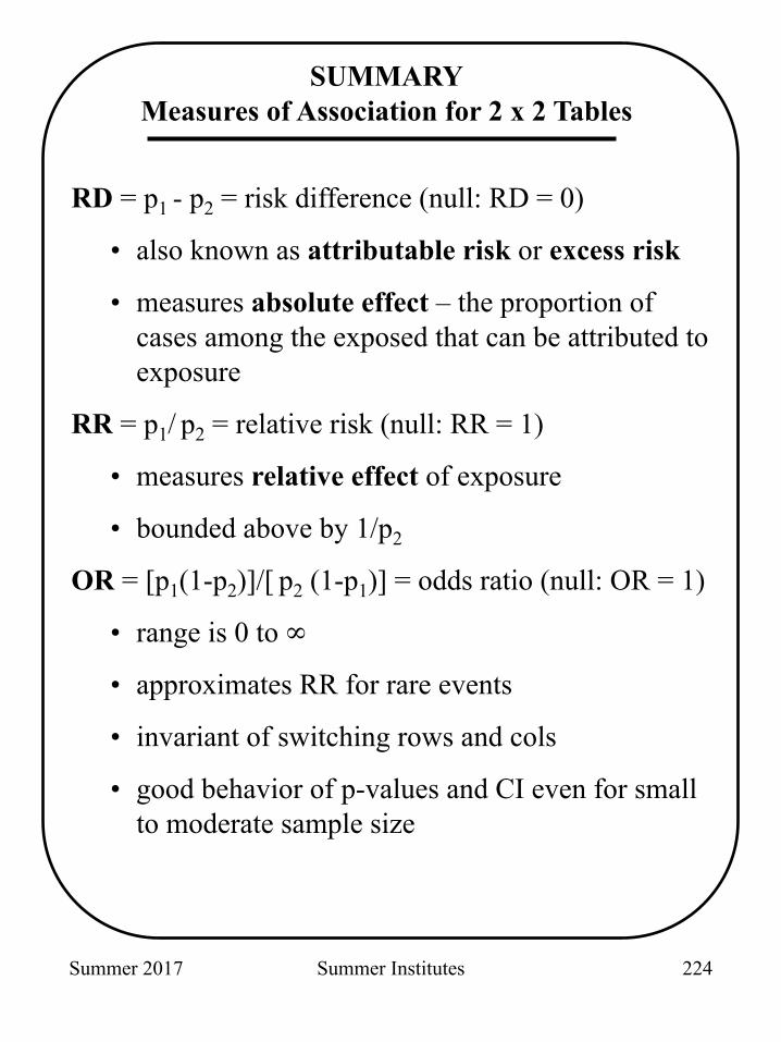
SUMMARY Measures of Association for 2 x 2 Tables

RD = p1 - p2 = risk difference (null: RD = 0)

•  also known as attributable risk or excess risk

•  measures absolute effect – the proportion of cases among the exposed that can be attributed to exposure

RR = p1/ p2 = relative risk (null: RR = 1)

•  measures relative effect of exposure

•  bounded above by 1/p2

OR = [p1(1-p2)]/[ p2 (1-p1)] = odds ratio (null: OR = 1)

•  range is 0 to ∞

•  approximates RR for rare events

•  invariant of switching rows and cols

•  good behavior of p-values and CI even for small to moderate sample size

224


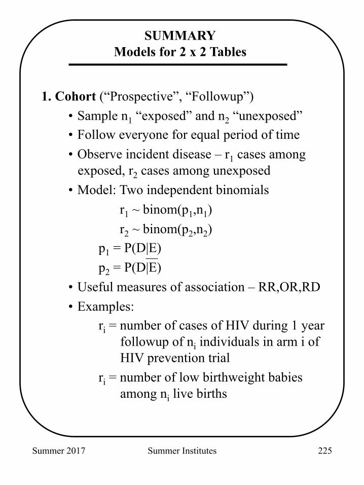
SUMMARY Models for 2 x 2 Tables

1.  Cohort (“Prospective”, “Followup”) •  Sample n1 “exposed” and n2 “unexposed” •  Follow everyone for equal period of time • Observe incident disease – r1 cases among

exposed, r2 cases among unexposed • Model: Two independent binomials

r1 ~ binom(p1,n1) r2 ~ binom(p2,n2)

p1 = P(D|E) p2 = P(D|E)

• Useful measures of association – RR,OR,RD •  Examples:

ri = number of cases of HIV during 1 year followup of ni individuals in arm i of HIV prevention trial

ri = number of low birthweight babies among ni live births

225


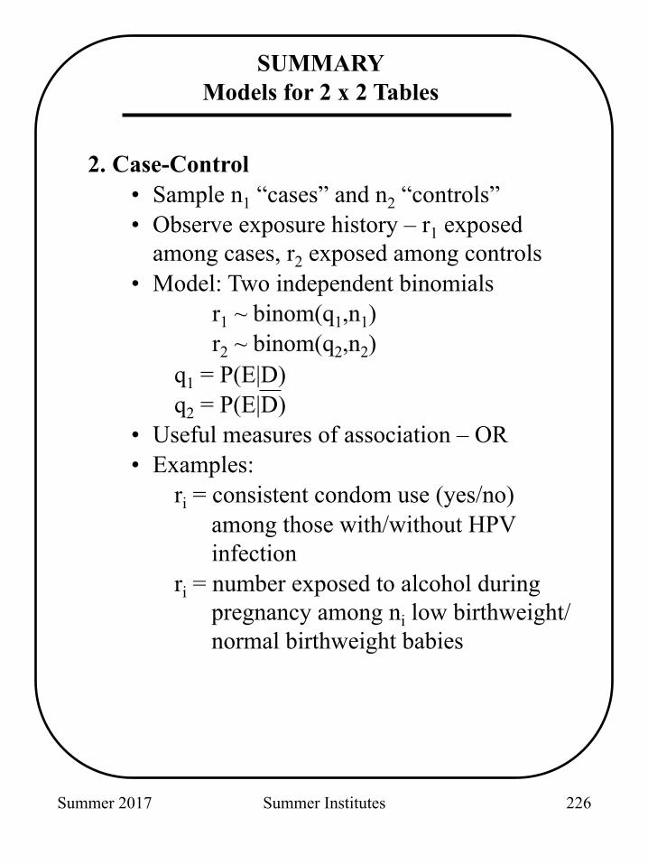
2.  Case-Control •  Sample n1 “cases” and n2 “controls” •  Observe exposure history – r1 exposed

among cases, r2 exposed among controls •  Model: Two independent binomials

r1 ~ binom(q1,n1) r2 ~ binom(q2,n2)

q1 = P(E|D) q2 = P(E|D)

•  Useful measures of association – OR •  Examples:

ri = consistent condom use (yes/no) among those with/without HPV infection

ri = number exposed to alcohol during pregnancy among ni low birthweight/normal birthweight babies


226


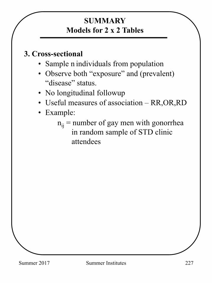
3.  Cross-sectional •  Sample n individuals from population •  Observe both “exposure” and (prevalent)

“disease” status. •  No longitudinal followup •  Useful measures of association – RR,OR,RD •  Example:

nij = number of gay men with gonorrhea in random sample of STD clinic attendees


227

Contingency Tables - University of Washington

Documents

Transcript of Contingency Tables - University of Washington