Methods of Describing Project Risk

Lecture No. 46Chapter 12Contemporary Engineering EconomicsCopyright © 2006

Chapter Opening Story – Oil Forecasts Are a Roll of the Dice Suppose that your

proposed project depends on the price of oil (common to airline industry, UPS, FedEx, and any petroleum-based manufacturing industry).

How would you factor the fluctuation and uncertainty into the analysis?

Origins of Project Risk

Risk: the potential for loss

Project Risk: variability in a project’s NPW

Risk Analysis: The assignment of probabilities to the various outcomes of an investment project

Methods of Describing Project Risk

Sensitivity Analysis: a procedure of identifying the project variables which, when varied, have the greatest effect on project acceptability.

Break-Even Analysis: a procedure of identifying the value of a particular project variable that causes the project to exactly break even.

Scenario Analysis: a procedure of comparing a “base case” to one or more additional scenarios, such as best and worst cases, to identify the extreme and most likely project outcomes.

Sensitivity Analysis – Example 12.1 Transmission-Housing Project by Boston Metal Company Financial Facts:

Known with Great Confidence Required investment = $125,000 Project Life = 5 years Income tax rate = 40% MARR = 15%

Unknown but Predictable (Most Likely Values) Unit variable cost = $15 per unit Number of units = 2,000 units Unit Price = $50 per unit Salvage value = $40,000 Fixed cost = $10,000/Yr

Required: Determine the acceptability of the investment

Develop a Project Cash Flow Statement Using Most-Likely Estimates – “Base Case”

0 1 2 3 4 5

Revenues:

Unit Price 50 50 50 50 50

Demand (units) 2,000 2,000 2,000 2,000 2,000

Sales revenue $100,000 $100,000 $100,000 $100,000 $100,000

Expenses:

Unit variable cost $15 $15 $15 $15 $15

Variable cost 30,000 30,000 30,000 30,000 30,000

Fixed cost 10,000 10,000 10,000 10,000 10,000

Depreciation 17,863 30,613 21,863 15,613 5,575

Taxable Income $42,137 $29,387 $38,137 $44,387 $54,425

Income taxes (40%) 16,855 11,755 15,255 17,755 21,770

Net Income $25,282 $17,632 $22,882 $26,632 $32,655

Cash Flow StatementCash Flow Statement

0 1 2 3 4 5

Operating activities

Net income 25,282 17,632 22,882 26,632 32,655

Depreciation 17,863 30,613 21,863 15,613 5,575

Investment activities

Investment (125,000)

Salvage 40,000

Gains tax (2,611)

Net cash flow ($125,500) $43,145 $48,245 $44,745 $42,245 $75,619

Developing an Excel Worksheet to Conduct Sensitivity Analysis

% deviationfrom the base

Sensitivity Analysis for Five Key Input Variables

Deviation -20% -15% -10% -5% 0% 5% 10% 15% 20%

Unit price $57 $9,999 $20,055 $30,111 $40,169 $50,225 $60,281 $70,337 $80,393

Demand 12,010 19,049 26,088 33,130 40,169 47,208 54,247 61,286 68,325

Variable cost 52,236 49,219 46,202 43,186 40,169 37,152 34,135 31,118 28,101

Fixed cost 44,191 43,185 42,179 41,175 40,169 39,163 38,157 37,151 36,145

Salvage value 37,782 38,378 38,974 39,573 40,169 40,765 41,361 41,957 42,553

Base

-20% -15% -10% -5% 0% 5% 10% 15% 20%

$100,000

90,000

80,000

70,000

60,000

50,000

40,000

30,000

20,000

10,000

0

-10,000

Base

Unit Price

Demand

Salvage value

Fixed cost

Variable cost

Sensitivity Graph (Spider Graph)

Break-Even Analysis

Breakeven analysis is a tool used to determine when a business will be able to cover all its expenses and begin to make a profit from a project.

Excel using a Goal Seek function

Analytical Approach

Using a Goal Seek Function in Excel

Goal Seek

Set cell:

To value:

By changing cell:

Ok Cancel

? X

$F$5

0

$B$6

NPW

Breakeven Value

Demand

Break-Even Analysis (Example 12.2) 1

23456789

1011121314151617181920212223242526272829303132333435363738394041

A B C D E F G

Example 10.3 Break-Even Analysis

Input Data (Base): Output Analysis:

Unit Price ($) 50$ Output (NPW) $0Demand 1429.39Var. cost ($/unit) 15$ Fixed cost ($) 10,000$ Salvage ($) 40,000$ Tax rate (%) 40%MARR (%) 15%

0 1 2 3 4 5Income Statement Revenues: Unit Price 50$ 50$ 50$ 50$ 50$ Demand (units) 1429.39 1429.39 1429.39 1429.39 1429.39 Sales Revenue 71,470$ 71,470$ 71,470$ 71,470$ 71,470$ Expenses: Unit Variable Cost 15$ 15$ 15$ 15$ 15$ Variable Cost 21,441 21,441 21,441 21,441 21,441 Fixed Cost 10,000 10,000 10,000 10,000 10,000 Depreciation 17,863 30,613 21,863 15,613 5,581

Taxable Income 22,166$ 9,416$ 18,166$ 24,416$ 34,448$ Income Taxes (40%) 8,866 3,766 7,266 9,766 13,779

Net Income 13,299$ 5,649$ 10,899$ 14,649$ 20,669$

Cash Flow StatementOperating Activities: Net Income 13,299 5,649 10,899 14,649 20,669 Depreciation 17,863 30,613 21,863 15,613 5,581 Investment Activities: Investment (125,000) Salvage 40,000 Gains Tax (2,613)

Net Cash Flow (125,000)$ 31,162$ 36,262$ 32,762$ 30,262$ 63,636$

Goal SeekFunctionParameters

12.2

Analytical Approach Unknown Sales Units (X)

0 1 2 3 4 5

Cash Inflows:

Net salvage 37,389

X(1-0.4)($50) 30X 30X 30X 30X 30X

0.4 (dep) 7,145 12,245 8,745 6,245 2,230

Cash outflows:

Investment -125,000

-X(1-0.4)($15) -9X -9X -9X -9X -9X

-(0.6)($10,000) -6,000 -6,000 -6,000 -6,000 -6,000

Net Cash Flow -125,000 21X +

1,145

21X + 6,245

21X +

2,745

21X +

245

21X +

33,617

PW of cash inflows

PW(15%)Inflow= (PW of after-tax net revenue)

+ (PW of net salvage value)

+ (PW of tax savings from depreciation

= 30X(P/A, 15%, 5) + $37,389(P/F, 15%, 5) + $7,145(P/F, 15%,1) + $12,245(P/F, 15%, 2)

+ $8,745(P/F, 15%, 3) + $6,245(P/F, 15%, 4)

+ $2,230(P/F, 15%,5)

= 30X(P/A, 15%, 5) + $44,490

= 100.5650X + $44,490o PW of cash outflows:

PW(15%)Outflow = (PW of capital expenditure_ + (PW) of after-tax expenses= $125,000 + (9X+$6,000)(P/A, 15%, 5)= 30.1694X + $145,113

PW of Cash Flows

The NPW:PW (15%) = 100.5650X + $44,490

- (30.1694X + $145,113)=70.3956X - $100,623.

Breakeven volume:

PW (15%) = 70.3956X - $100,623 = 0

Xb =1,430 units.

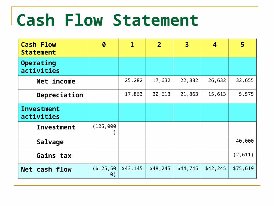
NPW and Breakeven Volume

NPW as a Function of Demand (X)

Demand

PW of

inflow

PW of

Outflow NPW

X 100.5650X

- $44,490

30.1694X

+ $145,113

70.3956X

-$100,623

0 $44,490 $145,113 -100,623

500 94,773 160,198 -65,425

1000 145,055 175,282 -30,227

1429 188,197 188,225 -28

1430 188,298 188,255 43

1500 195,338 190,367 4,970

2000 245,620 205,452 40,168

2500 295,903 220,537 75,366

Outflow

0 300 600 900 1200 1500 1800 2100 2400

$350,000

300,000

250,000

200,000

150,000

100,000

50,000

0

-50,000

-100,000

Profit

Loss

Break-even Volume

Xb =

1430

Annual Sales Units (X)

PW

(1

5%)

Inflow

Break-Even Chart – Break-Even Sales Volume at 1,430 Units

Scenario Analysis

Scenario analysis is a process of analyzing possible future events by considering alternative possible outcomes (scenarios). The analysis is designed to allow improved decision-making by allowing more complete consideration of outcomes and their implications. Source: Wikipedia

Example 12.3 Scenario Analysis

Variable

Considered

Worst-

Case

Scenario

Most-Likely-Case

Scenario

Best-Case

Scenario

Unit demand 1,600 2,000 2,400

Unit price ($) 48 50 53

Variable cost ($) 17 15 12

Fixed Cost ($) 11,000 10,000 8,000

Salvage value ($) 30,000 40,000 50,000

PW (15%) -$5,856 $40,169 $104,295