Contaminant Transportinthe TheoryandModeling · Contaminant Transportinthe UnsaturatedZone...

JACQ: “4316_c022” — 2006/5/26 — 19:26 — page 1 — #1

22Contaminant

Transport in theUnsaturated Zone

Theory and Modeling

Jirí ŠimunekUniversity of California Riverside

Martinus Th. vanGenuchtenGeorge E. Brown, Jr, SalinityLaboratory, USDA-ARS

22.1 Introduction. . . . . . . . . . . . . . . . . . . . . . . . . . . . . . . . . . . . . . . . . . . . . . 22-122.2 Variably Saturated Water Flow . . . . . . . . . . . . . . . . . . . . . . . . . . 22-3

Mass Balance Equation • Uniform Flow • Preferential Flow

22.3 Solute Transport . . . . . . . . . . . . . . . . . . . . . . . . . . . . . . . . . . . . . . . . . 22-8Transport Processes • Advection–Dispersion Equations •Nonequilibrium Transport • Stochastic Models •Multicomponent Reactive Solute Transport • MultiphaseFlow and Transport • Initial and Boundary Conditions

22.4 Analytical Models . . . . . . . . . . . . . . . . . . . . . . . . . . . . . . . . . . . . . . . . 22-22Analytical Approaches • Existing Models

22.5 Numerical Models . . . . . . . . . . . . . . . . . . . . . . . . . . . . . . . . . . . . . . . 22-27Numerical Approaches • Existing Models

22.6 Concluding Remarks . . . . . . . . . . . . . . . . . . . . . . . . . . . . . . . . . . . . 22-36References . . . . . . . . . . . . . . . . . . . . . . . . . . . . . . . . . . . . . . . . . . . . . . . . . . . . . . . 22-38

22.1 Introduction

Human society during the past several centuries has created a large number of chemical substances thatoften find their way into the environment, either intentionally applied during agricultural practices,unintentionally released from leaking industrial and municipal waste disposal sites, or stemming fromresearch or weapons production related activities. As many of these chemicals represent a significanthealth risk when they enter the food chain, contamination of both surface and subsurface water supplieshas become a major issue. Modern agriculture uses an unprecedented number of chemicals, both inplant and animal production. A broad range of fertilizers, pesticides and fumigants are now routinelyapplied to agricultural lands, thus making agriculture one of the most important sources for non-pointsource pollution. The same is true for salts and toxic trace elements, which are often an unintendedconsequence of irrigation in arid and semiarid regions. While many agricultural chemicals are generallybeneficial in surface soils, their leaching into the deeper vadose zone and groundwater may pose seriousproblems. Thus, management processes are being sought to keep fertilizers and pesticides in the root

22-1

JACQ: “4316_c022” — 2006/5/26 — 19:26 — page 2 — #2

22-2 The Handbook of Groundwater Engineering

zone and prevent their transport into underlying or down-gradient water resources. Agriculture alsoincreasingly uses a variety of pharmaceuticals and hormones in animal production many of which, alongwith pathogenic microorganisms, are being released to the environment through animal waste. Animalwaste and wash water effluent, in turn, is frequently applied to agricultural lands. Potential concerns aboutthe presence of pharmaceuticals and hormones in the environment include: (1) abnormal physiologicalprocesses and reproductive impairment; (2) increased incidences of cancer; (3) development of antibioticresistant bacteria; and (4) increased toxicity of chemical mixtures. While the emphasis above is mostly onnon-point source pollution by agricultural chemicals, similar problems arise with point-source pollutionfrom industrial and municipal waste disposal sites, leaking underground storage tanks, chemicals spills,nuclear waste repositories, and mine tailings, among other sources.

Mathematical models should be critical components of any effort to optimally understand and quantifysite-specific subsurface water flow and solute transport processes. For example, models can be helpful toolsfor designing, testing and implementing soil, water, and crop management practices that minimize soiland water pollution. Models are equally needed for designing or remediating industrial waste disposal sitesand landfills, or for long-term stewardship of nuclear waste repositories. A large number of specializednumerical models now exist to simulate the different processes at various levels of approximation and fordifferent applications.

Increasing attention is being paid recently to the unsaturated or vadose zone where much of thesubsurface contamination originates, passes through, or can be eliminated before it contaminates surfaceand subsurface water resources. Sources of contamination often can be more easily remediated in thevadose zone, before contaminants reach the underlying groundwater. Other chapters in this Handbookdeal with water flow (Chapters xx) and solute transport (Chapters xx) in fully saturated (groundwater)systems and with water flow in the unsaturated zone (Chapter 5). The focus of this chapter thus will beon mathematical descriptions of transport processes in predominantly variably saturated media.

Soils are generally defined as the biologically active layer at the surface of the earth’s crust that is madeup of a heterogeneous mixture of solid, liquid, and gaseous material, as well as containing a diversecommunity of living organisms (Jury and Horton, 2004). The vadose (unsaturated) zone is defined asthe layer between the land surface and the permanent (seasonal) groundwater table. While pores betweensolid grains are fully filled with water in the saturated zone (groundwater), pores in the unsaturated zoneare only partially filled with water, with the remaining part of the pore space occupied by the gaseousphase. The vadose zone is usually only partially saturated, although saturated regions may exist, such aswhen perched water is present above a low-permeable fine-textured (clay) layer or a saturated zone behindthe infiltration front during or after a high-intensity rainfall event.

As the transport of contaminants is closely linked with the water flux in soils and rocks making up thevadose zone, any quantitative analysis of contaminant transport must first evaluate water fluxes into andthrough the vadose zone. Water typically enters the vadose zone in the form of precipitation or irrigation(Figure 22.1), or by means of industrial and municipal spills. Some of the rainfall or irrigation watermay be intercepted on the leaves of vegetation. If the rainfall or irrigation intensity is larger than theinfiltration capacity of the soil, water will be removed by surface runoff, or will accumulate at the soilsurface until it evaporates back to the atmosphere or infiltrates into the soil. Part of this water is returnedto the atmosphere by evaporation. Some of the water that infiltrates into the soil profile may be takenup by plant roots and eventually returned to the atmosphere by plant transpiration. The processes ofevaporation and transpiration are often combined into the single process of evapotranspiration. Onlywater that is not returned to the atmosphere by evapotranspiration may percolate to the deeper vadosezone and eventually reach the groundwater table. If the water table is close enough to the soil surface, theprocess of capillary rise may move water from the groundwater table through the capillary fringe towardthe root zone and the soil surface.

Because of the close linkage between water flow and solute transport, we will first briefly focus on thephysics and mathematical description of water flow in the vadose zone (Section 22.2). An overview is givenof the governing equations for water flow in both uniform (Section 22.2.2) and structured (Section 22.2.3)media. This section is followed by a discussion of the governing solute transport equations (Section 22.3),

JACQ: “4316_c022” — 2006/5/26 — 19:26 — page 3 — #3

Contaminant Transport in the Unsaturated Zone Theory and Modeling 22-3

Transpiration

Rainfall

Interception

Evaporation

Irrigation

Runoff

Root wateruptake

Deep drainageCapillary rise

Groundwater recharge

Water table

Uns

atur

ated

zon

e

zone

Sat

urat

ed

Roo

t zon

e

Sto

rage

FIGURE 22.1 Schematic of water fluxes and various hydrologic components in the vadose zone.

again for both uniform (Section 22.3.2) and structured (fractured) (Section 22.3.3) media. We alsobriefly discuss alternative formulations for colloid (Section 22.3.3.2.2) and colloid-facilitated transport(Section 22.3.3.3), multicomponent geochemical transport (Section 22.3.5), and stochastic approachesfor solute transport (Section 22.3.4). This is followed by a discussion of analytical (Section 22.4) andnumerical (Section 22.5) approaches for solving the governing flow and transport equations, and anoverview of computer models currently available for simulating vadose zone flow and transport processes(Sections 22.4.2 and 22.5.2).

22.2 Variably Saturated Water Flow

In this section, we briefly present the equations governing variably saturated water flow in the subsur-face. More details about this topic, including the description of the soil hydraulic properties and theirconstitutive relationship, are given in Chapter xx. Traditionally, descriptions of variably saturated flowin soils are based on the Richards (1931) equation, which combines the Darcy–Buckingham equationfor the fluid flux with a mass balance equation. The Richards equation typically predicts a uniform flowprocess in the vadose zone, although possibly modified macroscopically by spatially variable soil hydraulicproperties (e.g., as dictated by the presence of different soil horizons, but possibly also varying laterally).

JACQ: “4316_c022” — 2006/5/26 — 19:26 — page 4 — #4


Unfortunately, the vadose zone can be extremely heterogeneous at a range of scales, from the microscopic(e.g., pore scale) to the macroscopic (e.g., field or larger scale). Some of these heterogeneities can leadto a preferential flow process that macroscopically is very difficult to capture with the standard Richardsequation. One obvious example of preferential flow is the rapid movement of water and dissolved solutesthrough macropores (e.g., between soil aggregates, or created by earthworms or decayed root channels)or rock fractures, with much of the water bypassing (short-circuiting) the soil or rock matrix. However,many other causes of preferential flow exist, such as flow instabilities caused by soil textural changes orwater repellency (Hendrickx and Flury, 2001; Šimunek et al. 2003; Ritsema and Dekker 2005), and lateralfunneling of water due to inclined or other textural boundaries (e.g., Kung 1990). Alternative ways ofmodeling preferential flow are discussed in a later section. Here we first focus on the traditional approachfor uniform flow as described with the Richards equation.

22.2.1 Mass Balance Equation

Water flow in variably saturated rigid porous media (soils) is usually formulated in terms of a mass balanceequation of the form:

∂θ

∂t= −∂qi

∂xi− S (22.1)

where θ is the volumetric water content [L3L−3], t is time [T], xi is the spatial coordinate [L], qi is thevolumetric flux density [LT−1], and S is a general sink/source term [L3L−3T−1], for example, to accountfor root water uptake (transpiration). Equation 22.1 is often referred to as the mass conservation equationor the continuity equation. The mass balance equation in general states that the change in the watercontent (storage) in a given volume is due to spatial changes in the water flux (i.e., fluxes in and out ofsome unit volume of soil ) and possible sinks or sources within that volume. The mass balance equationmust be combined with one or several equations describing the volumetric flux density (q) to produce thegoverning equation for variably saturated flow. The formulations of the governing equations for differenttypes of flow (uniform and preferential flow) are all based on this continuity equation.

22.2.2 Uniform Flow

Uniform flow in soils is described using the Darcy–Buckingham equation:

qi = −K (h)

(K A

ij∂h

∂xj+ K A

iz

)(22.2)

where K is the unsaturated hydraulic conductivity [LT−1], and K Aij are components of a dimensionless

anisotropy tensor KA (which reduces to the unit matrix when the medium is isotropic). The Darcy–Buckingham equation is formally similar to Darcy’s equation, except that the proportionality constant(i.e., the unsaturated hydraulic conductivity) in the Darcy–Buckingham equation is a nonlinear functionof the pressure head (or water content), while K (h) in Darcy’s equation is a constant equal to the saturatedhydraulic conductivity, Ks (e.g., see discussion by Narasimhan [2005]).

Combining the mass balance Equation 22.1 with the Darcy–Buckingham Equation22.2 leads to thegeneral Richards equation (Richards, 1931)

∂θ(h)

∂t= ∂

∂xi

[K (h)

(K A

ij∂h

∂xj+ K A

iz

)]− S(h) (22.3)

This partial differential equation is the equation governing variably saturated flow in the vadose zone.Because of its strongly nonlinear makeup, only a relatively few simplified analytical solutions can bederived. Most practical applications of Equation 22.3 require a numerical solution, which can be obtainedusing a variety of numerical methods such as finite differences or finite elements (Section 22.5a).

JACQ: “4316_c022” — 2006/5/26 — 19:26 — page 5 — #5


Equation 22.3 is generally referred to as the mixed form of the Richards equation as it contains twodependent variables, that is, the water content and the pressure head. Various other formulations of theRichards equation are possible.

22.2.3 Preferential Flow

Increasing evidence exists that variably saturated flow in many field soils is not consistent with theuniform flow pattern typically predicted with the Richards equations (Flury et al., 1994; Hendrickx andFlury, 2001). This is due to the presence of macropores, fractures, or other structural voids or biologicalchannels through which water and solutes may move preferentially, while bypassing a large part of thematrix pore-space. Preferential flow and transport processes are probably the most frustrating in termsof hampering accurate predictions of contaminant transport in soils and fractured rocks. Contrary touniform flow, preferential flow results in irregular wetting of the soil profile as a direct consequence ofwater moving faster in certain parts of the soil profile than in others. Hendrickx and Flury (2001) definedpreferential flow as constituting all phenomena where water and solutes move along certain pathways,while bypassing a fraction of the porous matrix. Water and solutes for these reasons can propagate quicklyto far greater depths, and much faster, than would be predicted with the Richards equation describinguniform flow.

The most important causes of preferential flow are the presence of macropores and other structuralfeatures, development of flow instabilities (i.e., fingering) caused by profile heterogeneities or waterrepellency (Hendrickx et al., 1993), and funneling of flow due to the presence of sloping soil layers thatredirect downward water flow. While the latter two processes (i.e., flow instability and funneling) areusually caused by textural differences and other factors at scales significantly larger than the pore scale,macropore flow and transport are usually generated at the pore or slightly larger scales, including scaleswhere soil structure first manifests itself (i.e., the pedon scale) (Šimunek et al., 2003).

Uniform flow in granular soils and preferential flow in structured media (both macroporous soils andfractured rocks) can be described using a variety of single-porosity, dual-porosity, dual-permeability,multi-porosity, and multi-permeability models (Richards, 1931; Pruess and Wang, 1987; Gerke and vanGenuchten, 1993a; Gwo et al., 1995; Jarvis, 1998; Šimunek et al., 2003, 2005). While single-porositymodels assume that a single pore system exists that is fully accessible to both water and solute, dual-porosity and dual-permeability models both assume that the porous medium consists of two interactingpore regions, one associated with the inter-aggregate, macropore, or fracture system, and one comprisingthe micropores (or intra-aggregate pores) inside soil aggregates or the rock matrix. Whereas dual-porositymodels assume that water in the matrix is stagnant, dual-permeability models allow also for water flowwithin the soil or rock matrix.

Figure 22.2 illustrates a hierarchy of conceptual formulations that can be used to model variablysaturated water flow and solute transport in soils. The simplest formulation (Figure 22.2a) is a single-porosity (equivalent porous medium) model applicable to uniform flow in soils. The other modelsapply in some form or another to preferential flow or transport. Of these, the dual-porosity modelof Figure 22.2c assumes the presence of two pore regions, with water in one region being immobileand in the other region mobile. This model allows the exchange of both water and solute between thetwo regions (Šimunek et al., 2003). Conceptually, this formulation views the soil as consisting of a soilmatrix containing grains/aggregates with a certain internal microporosity (intra-aggregate porosity) anda macropore or fracture domain containing the larger pores (inter-aggregate porosity). While water andsolutes are allowed to move through the larger pores and fractures, they can also flow in and out ofaggregates. By comparison, the intra-aggregate pores represent immobile pockets that can exchange,retain, and store water and solutes, but do not contribute to advective (or convective) flow. Models thatassume mobile–immobile flow regions (Figure 22.2b) are conceptually somewhere in between the single-and dual-porosity models. While these models assume that water will move similarly as in the uniformflow models, the liquid phase for purposes of modeling solute transport is divided in terms of mobile andimmobile fractions, with solutes allowed to move by advection and dispersion only in the mobile fraction

JACQ: “4316_c022” — 2006/5/26 — 19:26 — page 6 — #6


(a) Uniform flow

Water Water Immob

Immob.Immob.

Water Water

SoluteSoluteSoluteSolute

Mobile

MobileMobile

Slow

Slow

Fast

Fast

(b) Mobile-immobile water (c) Dual-porosity (d) Dual-permeability

� = �im + �mo� � = �im + �mo � = �m + �f

FIGURE 22.2 Conceptual models of water flow and solute transport (θ is the water content, θmo and θim in (b) and(c) are water contents in the mobile and immobile flow regions, respectively, and θm and θf in (d) are water contentsin the matrix and macropore (fracture) regions, respectively).

and between the two pore regions. This model has long been applied to solute transport studies (e.g., vanGenuchten and Wierenga, 1976).

Finally, dual-permeability models (Figure 22.2d) are those in which water can move in both the inter-and intra-aggregate pore regions (and matrix and fracture domains). These models in various forms arenow also becoming increasingly popular (Pruess and Wang, 1987; Gerke and van Genuchten, 1993a; Jarvis,1994; Pruess, 2004). Available dual-permeability models differ mainly in how they implement water flowin and between the two pore regions (Šimunek et al., 2003). Approaches to calculating water flow in themacropores or inter-aggregate pores range from those invoking Poiseuille’s equation (Ahuja and Hebson,1992), the Green and Ampt or Philip infiltration models (Ahuja and Hebson, 1992), the kinematic waveequation (Germann, 1985; Germann and Beven, 1985; Jarvis, 1994), and the Richards equation (Gerkeand van Genuchten, 1993a). Multi-porosity and multi-permeability models (not shown in Figure 22.2)are based on the same concept as dual-porosity and dual-permeability models, but include additionalinteracting pore regions (e.g., Gwo et al., 1995; Hutson and Wagenet, 1995). These models can be readilysimplified to the dual-porosity/permeability approaches. Recent reviews of preferential flow processes andavailable mathematical models are provided by Hendrickx and Flury (2001) and Šimunek et al. (2003),respectively.

22.2.3.1 Dual-Porosity Models

Dual-porosity models assume that water flow is restricted to macropores (or inter-aggregate pores andfractures), and that water in the matrix (intra-aggregate pores or the rock matrix) does not move at all.This conceptualization leads to two-region type flow and transport models (van Genuchten and Wierenga,1976) that partition the liquid phase into mobile (flowing, inter-aggregate), θmo, and immobile (stagnant,intra-aggregate), θim, regions [L3L−3]:

θ = θmo + θim (22.4)

The dual-porosity formulation for water flow can be based on a mixed formulation of the RichardsEquation 22.3 to describe water flow in the macropores (the preferential flow pathways) and a massbalance equation to describe moisture dynamics in the matrix as follows (Šimunek et al., 2003):

∂θmo(hmo)

∂t= ∂

∂xi

[K (hmo)

(K A

ij∂hmo

∂xj+ K A

iz

)]− Smo(hmo)− �w

∂θim(him)

∂t= −Sim(him)+ �w

(22.5)

JACQ: “4316_c022” — 2006/5/26 — 19:26 — page 7 — #7


where Sim and Smo are sink terms for both regions [T−1], and �w is the transfer rate for water from theinter- to the intra-aggregate pores [T−1].

Several of the above dual-porosity features were recently included in the HYDRUS software packages(Šimunek et al., 2003, 2005). Examples of their application to a range of laboratory and field data involvingtransient flow and solute transport are given by Šimunek et al. (2001), Zhang et al. (2004), Köhne et al.(2004a, 2005), Kodešová et al. (2005), and Haws et al. (2005).

22.2.3.2 Dual-Permeability Models

Different types of dual-permeability approaches may be used to describe flow and transport in structuredmedia. While several models invoke similar governing equations for flow in the fracture and matrixregions, others use different formulations for the two regions. A typical example of the first approach isthe work of Gerke and van Genuchten (1993a, 1996) who applied Richards equations to each of two poreregions. The flow equations for the macropore (fracture) (subscript f) and matrix (subscript m) poresystems in their approach are given by:

∂θf (hf )

∂t= ∂

∂xi

[Kf (hf )

(K A

ij∂hf

∂xj+ K A

iz

)]− Sf (hf )− �w

w(22.6)

and∂θm(hm)

∂t= ∂

∂xi

[Km(hm)

(K A

ij∂hm

∂xj+ K A

iz

)]− Sm(hm)+ �w

1− w(22.7)

respectively, where w is the ratio of the volumes of the macropore (or fracture or inter-aggregrate)domain and the total soil system [−]. This approach is relatively complicated in that the model requirescharacterization of water retention and hydraulic conductivity functions (potentially of different form)for both pore regions, as well as the hydraulic conductivity function of the fracture–matrix interface.Note that the water contents θf and θm in Equation 22.6 and Equation 22.7 have different meanings thanin Equation 22.5 where they represented water contents of the total pore space (i.e., θ = θmo + θim),while here they refer to water contents of the two separate (fracture or matrix) pore domains such thatθ = wθf + (1− w)θm.

22.2.3.3 Mass Transfer

The rate of exchange of water between the macropore and matrix regions,�w, is a critical term in both thedual-porosity model (Equation 22.5) and the dual-permeability approach given by (Equation 22.6) and(Equation 22.7). Gerke and van Genuchten (1993a) assumed that the rate of exchange is proportional tothe difference in pressure heads between the two pore regions:

�w = αw(hf − hm) (22.8)

in whichαw is a first-order mass transfer coefficient [T−1]. For porous media with well-defined geometries,the first-order mass transfer coefficient, αw, can be defined as follows (Gerke and van Genuchten, 1993b):

αw = β

d2Kaγw (22.9)

where d is an effective diffusion path length [L] (i.e., half the aggregate width or half the fracture spacing),β is a shape factor that depends on the geometry [−], and γw (= 0.4) is a scaling factor [−] obtainedby matching the results of the first-order approach at the half-time level of the cumulative infiltrationcurve to the numerical solution of the horizontal infiltration equation (Gerke and van Genuchten, 1993b).Several other approaches based on water content of relative saturation differences have also been used(Šimunek et al., 2003).

JACQ: “4316_c022” — 2006/5/26 — 19:26 — page 8 — #8


22.3 Solute Transport

Similarly, as shown in Equation 22.1 for water flow, mathematical formulations for solute transport areusually based on a mass balance equation of the form:

∂CT

∂t= −∂JTi

∂xi− φ (22.10)

where CT is the total concentration of chemical in all forms [ML−3], JTi is the total chemical mass fluxdensity (mass flux per unit area per unit time) [ML−2T−1], and φ is the rate of change of mass per unitvolume by reactions or other sources (negative) or sinks (positive) such as plant uptake [ML−3T−1]. Inits most general interpretation, Equation 22.10 allows the chemical to reside in all three phases of thesoil (i.e., gaseous, liquid, and solid), permits a broad range of transport mechanisms (including advectivetransport, diffusion, and hydrodynamic dispersion in both the liquid and gaseous phases), and facilitatesany type of chemical reaction that leads to losses or gains in the total concentration.

While the majority of chemicals are present only in the liquid and solid phases, and as such aretransported in the vadose zone mostly only in and by water, some chemicals such as many organiccontaminants, ammonium, and all fumigants, can have a significant portion of their mass in the gaseousphase and are hence subject to transport in the gaseous phase as well. The total chemical concentrationcan thus be defined as:

CT = ρbs + θc + ag (22.11)

where ρb is the bulk density [ML−3], θ is the volumetric water content [L3L−3], a is the volumetric aircontent [L3L−3], and s[MM−1], c[ML−3], and g [ML−3] are concentrations in the solid, liquid, andgaseous phases, respectively. The solid phase concentration represents solutes sorbed onto sorption sitesof the solid phase, but can include solutes sorbed onto colloids attached to the solid phase or strained bythe porous system, and solutes precipitated onto or into the solid phase.

The reaction term φ of Equation 22.10 may represent various chemical or biological reactions that leadto a loss or gain of chemical in the soil system, such as radionuclide decay, biological degradation, anddissolution. In analytical and numerical models these reactions are most commonly expressed using zero-and first-order reaction rates as follows:

φ = ρbsµs + θcµw + agµg − ρbγs − θγw − aγg (22.12)

where µs,µw, and µg are first-order degradation constants in the solid, liquid, and gaseous phases [T−1],respectively, and γs [T−1], γw [ML−3T−1], and γg [ML−3T−1] are zero-order production constants in thesolid, liquid, and gaseous phases, respectively.

22.3.1 Transport Processes

When a solute is present in both the liquid and gaseous phase, then various transport processes in both ofthese phases may contribute to the total chemical mass flux:

JT = Jl + Jg (22.13)

where Jl and Jg represent solute fluxes in the liquid and gaseous phases [ML−2T−1], respectively. Notethat in Equation 22.13, and further below, we omitted the subscript i accounting for the direction of flow.The three main processes that can be active in both the liquid and gaseous phase are molecular diffusion,hydrodynamic dispersion, and advection (often also called convection). The solute fluxes in the two phases

JACQ: “4316_c022” — 2006/5/26 — 19:26 — page 9 — #9


are then the sum of fluxes due to these different processes:

Jl = Jlc + Jld + Jlh

Jg = Jgc + Jgd + Jgh

(22.14)

where the additional subscripts c, d, and h denote convection (or advection), molecular diffusion, andhydrodynamic dispersion, respectively.

22.3.1.1 Diffusion

Diffusion is a result of the random motion of chemical molecules. This process causes a solute to movefrom a location with a higher concentration to a location with a lower concentration. Diffusive transportcan be described using Fick’s law:

Jld = −θξl(θ)Dwl

∂c

∂z= −θDs

l

∂c

∂z

Jgd = −aξg(θ)Dwg∂g

∂z= −aDs

g∂g

∂z

(22.15)

where Dwl and Dw

g are binary diffusion coefficients of the solute in water and gas [L2T−1], respectively; Dsl

and Dsg are the effective diffusion coefficients in soil water and soil gas [L2T−1], respectively; and ξl and

ξg are tortuosity factors that account for the increased path lengths and decreased cross-sectional areasof the diffusing solute in both phases (Jury and Horton, 2004). As solute diffusion in soil water (air) isseverely hampered by both air (water) and solid particles, the tortuosity factor increases strongly withwater content (air content). Many empirical models have been suggested in the literature to account forthe tortuosity (e.g., Moldrup et al., 1998). Among these, the most widely used model for the tortuosityfactor is probably the equation of Millington and Quirk (1961) given by:

ξl(θ) = θ7/3

θ2s

(22.16)

where θs is the saturated water content (porosity) [L3L−3]. A similar equation may be used for thetortuosity factor of the gaseous phase by replacing the water content with the air content.

22.3.1.2 Dispersion

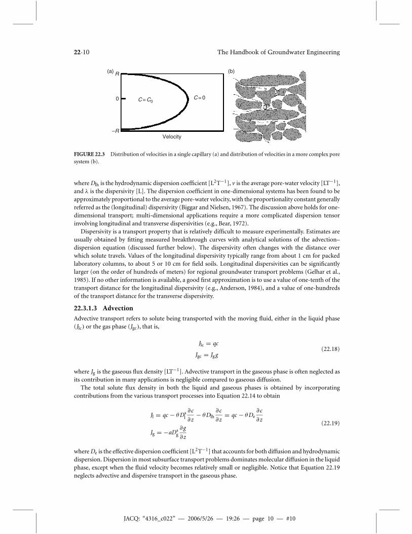
Dispersive transport of solutes results from the uneven distribution of water flow velocities within andbetween different soil pores (Figure 22.3). Dispersion can be derived from Newton’s law of viscosity whichstates that velocities within a single capillary tube follow a parabolic distribution, with the largest velocityin the middle of the pore and zero velocities at the walls (Figure 22.3a). Solutes in the middle of a pore,for this reason, will travel faster than solutes that are farther from the center. As the distribution of soluteions within a pore depends on their charge, as well as on the charge of pore walls, some solutes may movesignificantly faster than others. In some situations (i.e., for negatively charged anions in fine-texturedsoils, leading to anion exclusion), the solute may even travel faster than the average velocity of water (e.g.,Nielsen et al., 1986). Using Poiseuille’s law, one can further show that velocities in a capillary tube dependstrongly on the radius of the tube, and that the average velocity increases with the radius to the secondpower. As soils consist of pores of many different radii, solute fluxes in pores of different radii will besignificantly different, with some solutes again traveling faster than others (Figure 22.3b).

The above pore-scale dispersion processes lead to an overall (macroscopic) hydrodynamic dispersionprocess that mathematically can be described using Fick’s law in the same way as molecular diffusion,that is,

Jlh = −θDlh∂c

∂z= −θλv

∂c

∂z= −λq

∂c

∂z(22.17)

JACQ: “4316_c022” — 2006/5/26 — 19:26 — page 10 — #10


R

0

–R

C = C0C = 0

Velocity

(a) (b)

FIGURE 22.3 Distribution of velocities in a single capillary (a) and distribution of velocities in a more complex poresystem (b).

where Dlh is the hydrodynamic dispersion coefficient [L2T−1], v is the average pore-water velocity [LT−1],and λ is the dispersivity [L]. The dispersion coefficient in one-dimensional systems has been found to beapproximately proportional to the average pore-water velocity, with the proportionality constant generallyreferred as the (longitudinal) dispersivity (Biggar and Nielsen, 1967). The discussion above holds for one-dimensional transport; multi-dimensional applications require a more complicated dispersion tensorinvolving longitudinal and transverse dispersivities (e.g., Bear, 1972).

Dispersivity is a transport property that is relatively difficult to measure experimentally. Estimates areusually obtained by fitting measured breakthrough curves with analytical solutions of the advection–dispersion equation (discussed further below). The dispersivity often changes with the distance overwhich solute travels. Values of the longitudinal dispersivity typically range from about 1 cm for packedlaboratory columns, to about 5 or 10 cm for field soils. Longitudinal dispersivities can be significantlylarger (on the order of hundreds of meters) for regional groundwater transport problems (Gelhar et al.,1985). If no other information is available, a good first approximation is to use a value of one-tenth of thetransport distance for the longitudinal dispersivity (e.g., Anderson, 1984), and a value of one-hundredsof the transport distance for the transverse dispersivity.

22.3.1.3 Advection

Advective transport refers to solute being transported with the moving fluid, either in the liquid phase(Jlc) or the gas phase (Jgc), that is,

Jlc = qc

Jgc = Jgg(22.18)

where Jg is the gaseous flux density [LT−1]. Advective transport in the gaseous phase is often neglected asits contribution in many applications is negligible compared to gaseous diffusion.

The total solute flux density in both the liquid and gaseous phases is obtained by incorporatingcontributions from the various transport processes into Equation 22.14 to obtain

Jl = qc − θDsl

∂c

∂z− θDlh

∂c

∂z= qc − θDe

∂c

∂z

Jg = −aDsg∂g

∂z

(22.19)

where De is the effective dispersion coefficient [L2T−1] that accounts for both diffusion and hydrodynamicdispersion. Dispersion in most subsurface transport problems dominates molecular diffusion in the liquidphase, except when the fluid velocity becomes relatively small or negligible. Notice that Equation 22.19neglects advective and dispersive transport in the gaseous phase.

JACQ: “4316_c022” — 2006/5/26 — 19:26 — page 11 — #11


22.3.2 Advection–Dispersion Equations

22.3.2.1 Transport Equations

The equation governing transport of dissolved solutes in the vadose zone is obtained by combining thesolute mass balance (Equation 22.10) with equations defining the total concentration of the chemical(Equation 22.11) and the solute flux density (Equation 22.19) to give

∂(ρbs + θc + ag )

∂t= ∂

∂xi

(θDeij

∂c

∂xj

)+ ∂

∂xi

(aDs

gij∂g

∂xj

)− ∂

(qic)

∂xi− φ (22.20)

Notice that this equation is again written for multidimensional transport, and that Deij and Dsij are thus

components of the effective dispersion tensor in the liquid phase and a diffusion tensor in the gaseousphase [L2T−1], respectively.

Many different variants of Equation 22.20 can be found in the literature. For example, forone-dimensional transport of nonvolatile solutes, the equation simplifies to

∂(ρbs + θc)

∂t= ∂(θRc)

∂t= ∂

∂z

(θDe

∂c

∂z

)− ∂(qc)

∂z− φ (22.21)

where q is the vertical water flux density [LT−1] and R is the retardation factor [−]

R = 1+ ρb

θ

ds(c)

dc(22.22)

For transport of inert, nonadsorbing solutes during steady-state water flow we obtain

∂c

∂t= De

∂2c

∂z2− v

∂c

∂z(22.23)

The above equations are usually referred to as advection–dispersion equations (ADEs).

22.3.2.2 Linear and Nonlinear Sorption

The ADE given by Equation 22.20 contains three unknown concentrations (those for the liquid, solid,and gaseous phases), while Equation 22.21 contains two unknowns. To be able to solve these equations,additional information is needed that somehow relates these concentrations to each other. The mostcommon way is to assume instantaneous sorption and to use adsorption isotherms to relate the liquid andadsorbed concentrations. The simplest form of the adsorption isotherm is the linear isotherm given by

s = Kdc (22.24)

where Kd is the distribution coefficient [L3M−1]. One may verify that substitution of this equation intoEquation 22.22 leads to a constant value for the retardation factor (i.e., R = 1+ ρbKd/θ).

While the use of a linear isotherm greatly simplifies the mathematical description of solute transport,sorption and exchange are generally nonlinear and most often depend also on the presence of competingspecies in the soil solution. The solute retardation factor for nonlinear adsorption is not constant, as isthe case for linear adsorption, but changes as a function of concentration. Many models have been usedin the past to describe nonlinear sorption. The most commonly used nonlinear sorption models are thoseby Freundlich (1909) and Langmuir (1918) given by:

s = Kf cβ (22.25)

s = Kdc

1+ ηc(22.26)

JACQ: “4316_c022” — 2006/5/26 — 19:26 — page 12 — #12


0

0.2

0.4

0.6

0.8

1

1.2

1.4

Dissolved concentration [M/L3]

0 0.5 1 1.5 0 0.5 1 1.5

Sor

bed

conc

entr

atio

n [M

/M]

0.5

0.75

1

1.5

2

2.5

3

5

Increasing

0

0.1

0.2

0.3

0.4

0.5

0.6

0.7

0.8

0.9

1

Dissolved concentration [M/L3]

Sor

bed

conc

entr

atio

n [M

/M]

00.50.7511.522.535

Increasing

(a) (b)

FIGURE 22.4 Plots of the Freundlich adsorption isotherm given by (22.25), with Kd = 1 and β given in thecaption (a), and the Langmuir adsorption isotherm given by (22.26), with Kd = 1 and η given in the caption (b).

TABLE 22.1 Equilibrium Adsorption Equations (adapted from van Genuchten and Šimunek (1996))

Equation Model Reference

s = k1c + k2 Linear Lapidus and Amundson (1952)Lindstrom et al. (1967)

s = k1ck3

1+ k2ck3Freundlich–Langmuir Sips (1950), Šimunek et al. (1994, 2005)

s = k1c

1+ k2c+ k3c

1+ k4cDouble Langmuir Shapiro and Fried (1959)

s = k1cck2/k3 Extended Freundlich Sibbesen (1981)

s = k1c

1+ k2c + k3√

cGunary Gunary (1970)

s = k1ck2 − k3 Fitter–Sutton Fitter and Sutton (1975)

s = k1{1− [1+ k2ck3 ]k4 } Barry Barry (1992)

s = RT

k1ln(k2c) Temkin Bache and Williams (1971)

s = k1c exp(−2k2s) Lindstrom et al. (1971)van Genuchten et al. (1974)

s

sT= c[c + k1(cT − c) exp{k2(cT − 2c)}]−1 Modified Kielland Lai and Jurinak (1971)

k1, k2, k3, k4: empirical constants; R: universal gas constant; T : absolute temperature; cT: maximum soluteconcentration; sT : maximum adsorbed concentration.

Source: Adapted from van Genuchten, M.Th. and Šimunek, J. In P.E. Rijtema and V. Eliáš (Eds.), RegionalApproaches to Water Pollution in the Environment, NATO ASI Series: 2. Environment. Kluwer, Dordrecht, TheNetherlands, pp. 139–172, 1996.

respectively, where Kf [M−β L−3β] and β [−] are coefficients in the Freundlich isotherm, and η [L3M−1]is a coefficient in the Langmuir isotherm. Examples of linear, Freundlich and Langmuir adsorptionisotherms are given in Figure 22.4. Table 22.1 lists a range of linear and other sorption models frequentlyused in solute transport studies.

JACQ: “4316_c022” — 2006/5/26 — 19:26 — page 13 — #13


22.3.2.3 Volatilization

Volatilization is increasingly recognized as an important process affecting the fate of many organic chem-icals, including pesticides, fumigants, and explosives in field soils (Jury et al., 1983, 1984; Glotfelty andSchomburg, 1989). While many organic pollutants dissipate by means of chemical and microbiologicaldegradation, volatilization may be equally important for volatile substances, such as certain pesticides.The volatility of pesticides is influenced by many factors, including the physicochemical properties of thechemical itself as well-such environmental variables as temperature and solar energy. Even though only asmall fraction of a pesticide may exist in the gas phase, air-phase diffusion rates can sometimes be com-parable to liquid-phase diffusion as gas-phase diffusion is about four orders of magnitude greater thanliquid phase diffusion. The importance of gaseous diffusion relative to other transport processes dependsalso on the climate. For example, while transport of MTBE (gasoline oxygenate) is generally dominatedby liquid advection in humid areas, gaseous diffusion may be equally or more important in arid climates;this even though only about 2% of MTBE may be in the gas phase.

The general transport equation given by Equation 22.20 can be simplified considerably when assuminglinear equilibrium sorption and volatilization such that the adsorbed (s) and gaseous (g ) concentrationsare linearly related to the solution concentration (c) through the distribution coefficients, Kd in (22.24)and KH, that is,

g = KHc (22.27)

respectively, where KH is the dimensionless Henry’s constant [−]. Equation 22.20 for one-dimensionaltransport then has the form:

∂(ρbKd + θ + aKH)c

∂t= ∂

∂z

(θDe

∂c

∂z

)+ ∂

∂z

(aDs

gKH∂c

∂z

)− ∂

(qc)

∂x− φ (22.28)

or∂θRc

∂t= ∂

∂z

(θDE

∂c

∂z

)− ∂

(qc)

∂x− φ (22.29)

where the retardation factor R [−] and the effective dispersion coefficient DE [L2T−1] are defined asfollows:

R = 1+ ρbKd + aKH

θ

DE = De +aDs

gKH

θ

(22.30)

Jury et al. (1983, 1984) provided for many organic chemicals their distribution coefficients Kd, Henry’sconstants KH, and calculated percent mass present in each phase.

22.3.3 Nonequilibrium Transport

As equilibrium solute transport models often fail to describe experimental data, a large number ofdiffusion-controlled physical nonequilibrium and chemical-kinetic models have been proposed and usedto describe the transport of both non-adsorbing and adsorbing chemicals. Attempts to model nonequilib-rium transport usually involve relatively simple first-order rate equations. Nonequilibrium models haveused the assumptions of two-region (dual-porosity) type transport involving solute exchange betweenmobile and immobile liquid transport regions, and one-, two- or multi-site sorption formulations (e.g.,Nielsen et al., 1986; Brusseau, 1999). Models simulating the transport of particle-type pollutants, suchas colloids, viruses, and bacteria, often also use first-order rate equations to describe such processes asattachment, detachment, and straining. Nonequilibrium models generally have resulted in better descrip-tions of observed laboratory and field transport data, in part by providing additional degrees of freedomfor fitting observed concentration distributions.

JACQ: “4316_c022” — 2006/5/26 — 19:26 — page 14 — #14


22.3.3.1 Physical Nonequilibrium

22.3.3.1.1 Dual-Porosity and Mobile–Immobile Water ModelsThe two-region transport model (Figures 22.2b and Figure 22.2c) assumes that the liquid phase can bepartitioned into distinct mobile (flowing) and immobile (stagnant) liquid pore regions, and that soluteexchange between the two liquid regions can be modeled as a first-order exchange process. Using the samenotation as before, the two-region solute transport model is given by (van Genuchten and Wagenet, 1989;Toride et al., 1993):

∂θmocmo

∂t+ ∂f ρsmo

∂t= ∂

∂z

(θmoDmo

∂cmo

∂z

)− ∂qcmo

∂z− φmo − �s

∂θimcim

∂t+ ∂(1− f )ρsim

∂t= −φim + �s

(22.31)

for the mobile (macropores, subscript mo) and immobile (matrix, subscript im) domains, respectively,where f is the dimensionless fraction of sorption sites in contact with the mobile water [−], φmo andφim are reactions in the mobile and immobile domains [ML3T−1], respectively, and �s is the solutetransfer rate between the two regions [ML3T−1]. Notice that the same equations Equation 22.31 can beused to describe solute transport using both the mobile–immobile and dual-porosity models shown inFigures 22.2b and Figure 22.2c, respectively.

22.3.3.1.2 Dual-Permeability ModelAnalogous to Equations 22.6 and Equation 22.7 for water flow, the dual-permeability formulation forsolute transport can be based on advection–dispersion type equations for transport in both the fractureand matrix regions as follows (Gerke and van Genuchten, 1993a):

∂θf cf

∂t+ ∂ρsf

∂t= ∂

∂z

(θf Df

∂cf

∂z

)− ∂qf cf

∂z− φf − �s

w(22.32)

∂θmcm

∂t+ ∂ρsm

∂t= ∂

∂z

(θmDm

∂cm

∂z

)− ∂qmcm

∂z− φm − �s

1− w(22.33)

where the subscript f and m refer to the macroporous (fracture) and matrix pore systems, respectively; φf

and φm represent sources or sinks in the macroporous and matrix domains [ML3T−1], respectively; andw is the ratio of the volumes of the macropore-domain (inter-aggregate) and the total soil systems [−].Equation 22.32 and Equation 22.33 assume complete advective–dispersive type transport descriptions forboth the fractures and the matrix. Several authors simplified transport in the macropore domain, forexample, by considering only piston displacement of solutes (Ahuja and Hebson, 1992; Jarvis, 1994).

22.3.3.1.3 Mass TransferThe transfer rate, �s, in Equation 22.31 for solutes between the mobile and immobile domains in thedual-porosity models can be given as the sum of diffusive and advective fluxes, and can be written as

�s = αs(cmo − cim)+ �wc∗ (22.34)

where c∗ is equal to cmo for �w > 0 and cim for �w < 0, and αs is the first-order solute mass transfercoefficient [T−1]. Notice that the advection term of Equation 22.34 is equal to zero for the mobile–immobile model (Figure 22.2b) as the immobile water content in this model is assumed to be constant.However, �w may have a nonzero value in the dual-porosity model depicted in Figure 22.2c.

The transfer rate,�s, in Equation 22.32 and Equation 22.33 for solutes between the fracture and matrixregions is also usually given as the sum of diffusive and advective fluxes as follows (e.g., Gerke and vanGenuchten, 1996):

�s = αs(1− wm)(cf − cm)+ �wc∗ (22.35)

JACQ: “4316_c022” — 2006/5/26 — 19:26 — page 15 — #15


in which the mass transfer coefficient, αs [T−1], is of the form:

αs = β

d2Da (22.36)

where Da is an effective diffusion coefficient [L2T−1] representing the diffusion properties of the fracture–matrix interface.

Still more sophisticated models for physical nonequilibrium transport may be formulated. For example,Pot et al. (2005) and Köhne et al. (2006) considered a dual-permeability model that divides the matrixdomain further into mobile and immobile subregions and used this model successfully to simulate bromidetransport in laboratory soil columns at different flow rates or for transient flow conditions, respectively.

22.3.3.2 Chemical Nonequilibrium

22.3.3.2.1 Kinetic Sorption ModelsAn alternative to expressing sorption as an instantaneous process using algebraic equations (e.g., Equa-tion 22.24, Equation 22.25 or Equation 22.26) is to describe the kinetics of the reaction using ordinarydifferential equations. The most popular and simplest formulation of a chemically controlled kineticreaction arises when first-order linear kinetics is assumed:

∂s

∂t= αk(Kdc − s) (22.37)

where αk is a first-order kinetic rate coefficient [T−1]. Several other nonequilibrium adsorption expres-sions were also used in the past (see Table 2 in van Genuchten and Šimunek, 1996). Models based on thisand other kinetic expressions are often referred to as one-site sorption models.

As transport models assuming chemically controlled nonequilibrium (one-site sorption) generally didnot result in significant improvements in their predictive capabilities when used to analyze laboratorycolumn experiments, the one-site first-order kinetic model was further expanded into a two-site sorptionconcept that divides the available sorption sites into two fractions (Selim et al., 1976; van Genuchten andWagenet, 1989). In this approach, sorption on one fraction (type-1 sites) is assumed to be instantaneouswhile sorption on the remaining (type-2) sites is considered to be time-dependent. Assuming a linearsorption process, the two-site transport model is given by (van Genuchten and Wagenet, 1989)

∂(f ρbKd + θ)c∂t

= ∂

∂z

(θDe

∂ c

∂z

)− ∂

(qc)

∂z− φe

∂sk

∂t= αk[(1− f )Kdc − sk] − φk

(22.38)

where f is the fraction of exchange sites assumed to be at equilibrium [−], φe [ML3T−1] and φk

[MM−1T−1] are reactions in the equilibrium and nonequilibrium phases, respectively, and the sub-script k refers to kinetic (type-2) sorption sites. Note that if f = 0, the two-site sorption model reducesto the one-site fully kinetic sorption model (i.e., when only type-2 kinetic sites are present). On the otherhand, if f = 1, the two-site sorption model reduces to the equilibrium sorption model for which onlytype-1 equilibrium sites are present.

22.3.3.2.2 Attachment/Detachment ModelsAdditionally, transport equations may include provisions for kinetic attachment/detachment of solutesto the solid phase, thus permitting simulations of the transport of colloids, viruses, and bacteria. Thetransport of these constituents is generally more complex than that of other solutes in that they areaffected by such additional processes as filtration, straining, sedimentation, adsorption and desorption,growth, and inactivation. Virus, colloid, and bacteria transport and fate models commonly employ a

JACQ: “4316_c022” — 2006/5/26 — 19:26 — page 16 — #16


modified form of the ADE, in which the kinetic sorption equations are replaced with equations describingkinetics of colloid attachment and detachment as follows:

ρ∂s

∂t= θkaψc − kdρs (22.39)

where c is the (colloid, virus, bacteria) concentration in the aqueous phase [Nc L−3], s is the solid phase(colloid, virus, bacteria) concentration [Nc M−1], in which Nc is a number of (colloid) particles, ka isthe first-order deposition (attachment) coefficient [T−1], kd is the first-order entrainment (detachment)coefficient [T−1], andψ is a dimensionless colloid retention function [−]. The attachment and detachmentcoefficients in Equation 22.39 have been found to strongly depend upon water content, with attachmentsignificantly increasing as the water content decreases.

To simulate reductions in the attachment coefficient due to filling of favorable sorption sites,ψ is some-times assumed to decrease with increasing colloid mass retention. A Langmuirian dynamics (Adamczyket al., 1994) equation has been proposed for ψ to describe this blocking phenomenon:

ψ = smax − s

smax= 1− s

smax(22.40)

in which smax is the maximum solid phase concentration [NcM−1].A similar equation as Equation 22.39 was used by Bradford et al. (2003, 2004) to simulate the process of

pore straining. Bradford et al. (2003, 2004) hypothesized that the influence of straining and attachmentprocesses on colloid retention should be separated into two distinct components. They suggested thefollowing depth-dependent blocking coefficient for the straining process:

ψ =(

dc + z − z0

dc

)−β(22.41)

where dc is the diameter of the sand grains [L], z0 is the coordinate of the location where the strainingprocess starts [L] (the surface of the soil profile, or interface between soil layers), and β is an empiricalfactor (Bradford et al., 2003) [−].

The attachment coefficient is often calculated using filtration theory (Logan et al., 1995), a quasi-empirical formulation in terms of the median grain diameter of the porous medium (often termed thecollector), the pore-water velocity, and collector and collision (or sticking) efficiencies accounting forcolloid removal due to diffusion, interception, and gravitational sedimentation (Rajagopalan and Tien,1976; Logan et al., 1995):

ka = 3(1− θ)2dc

ηαv (22.42)

where dc is the diameter of the sand grains [L], α is the sticking efficiency (ratio of the rate of particlesthat stick to a collector to the rate they strike the collector) [−], v is the pore-water velocity [LT−1], and ηis the single-collector efficiency [−].

In related studies, Schijven and Hassanizadeh (2000) and Schijven and Šimunek (2002) used a two-site sorption model based on two equations (22.39) to successfully describe virus transport at both thelaboratory and field scale. Their model assumed that the sorption sites on the solid phase can be dividedinto two fractions with different properties and various attachment and detachment rate coefficients.

22.3.3.3 Colloid-Facilitated Solute Transport

There is an increasing evidence that many contaminants, including radionuclides (Von Gunten et al.,1988; Noell et al., 1998), pesticides (Vinten et al., 1983; Kan and Tomson, 1990, Lindqvist and Enfield,1992), heavy metals (Grolimund et al., 1996), viruses, pharmaceuticals (Tolls, 2001; Thiele-Bruhn, 2003),hormones (Hanselman et al., 2003), and other contaminants (Magee et al., 1991; Mansfeldt et al., 2004)are transported in the subsurface not only with moving water, but also sorbed to mobile colloids. As many

JACQ: “4316_c022” — 2006/5/26 — 19:26 — page 17 — #17


colloids and microbes are negatively charged and thus electrostatically repelled by negatively charged solidsurfaces, which may lead to an anion exclusion process, their transport may be slightly enhanced relativeto fluid flow. Size exclusion may similarly enhance the advective transport of colloids by limiting theirpresence and mobility to the larger pores (e.g., Bradford et al., 2003). The transport of contaminants sorbedto mobile colloids can thus significantly accelerate their transport relative to more standard advection–transport descriptions.

Colloid-facilitated transport is a relatively complicated process that requires knowledge of water flow,colloid transport, dissolved contaminant transport, and colloid-contaminant interaction. Transport andmass balance equations, hence, must be formulated not only for water flow and colloid transport, butalso for the total contaminant, for contaminant sorbed kinetically or instantaneously to the solid phase,and for contaminant sorbed to mobile colloids, to colloids attached to the soil solid phase, and to colloidsaccumulating at the air–water interface. Development of such a model is beyond the scope of this chapter.We refer interested readers to several manuscripts dealing with this topic: Mills et al. (1991), Corapciogluand Jiang (1993), Corapcioglu and Kim (1995), Jiang and Corapcioglu (1993), Noell et al. (1998), Saierset al. (1996), Saiers and Hornberger (1996), van de Weerd et al. (1998), and van Genuchten and Šimunek(2004).

22.3.4 Stochastic Models

Much evidence suggests that solutions of classical solute transport models, no matter how refined toinclude the most relevant chemical and microbiological processes and soil properties, often still fail toaccurately describe transport processes in most natural field soils. A major reason for this failure is the factthat the subsurface environment is overwhelmingly heterogeneous. Heterogeneity occurs at a hierarchy ofspatial and time scales (Wheatcraft and Cushman, 1991), ranging from microscopic scales involving time-dependent chemical sorption and precipitation/dissolution reactions, to intermediate scales involving thepreferential movement of water and chemicals through macropores or fractures, and to much larger scalesinvolving the spatial variability of soils across the landscape. Subsurface heterogeneity can be addressedin terms of process-based descriptions which attempt to consider the effects of heterogeneity at one orseveral scales. It can also be addressed using stochastic approaches that incorporate certain assumptionsabout the transport process in the heterogeneous system (e.g., Sposito and Barry, 1987; Dagan, 1989).In this section we briefly review several stochastic transport approaches, notably those using stream tubemodels and the transfer function approach.

22.3.4.1 Stream Tube Models

The downward movement of chemicals from the soil surface to an underlying aquifer may be describedstochastically by viewing the field as a series of independent vertical columns, often referred to as “streamtubes” (Figure 22.5), while solute mixing between the stream tubes is assumed to be negligible. Transport

V1

V2

V3Vn–1

Vn

FIGURE 22.5 Schematic illustration of the stream tube model (Toride et al., 1995).

JACQ: “4316_c022” — 2006/5/26 — 19:26 — page 18 — #18


in each tube may be described deterministically with the standard ADE, or modifications thereof to includeadditional geochemical and microbiological processes. Transport at the field scale is then implemented byconsidering the column parameters as realizations of a stochastic process, having a random distribution(Toride et al., 1995). Early examples are by Dagan and Bresler (1979) and Bresler and Dagan (1979) whoassumed that the saturated hydraulic conductivity had a lognormal distribution.

The stream tube model was implemented into the CXTFIT 2.0 program (Toride et al., 1995) for avariety of transport scenarios in which the pore-water velocity in combination with either the dispersioncoefficient, De, the distribution coefficient for linear adsorption, Kd, or the first-order rate coefficient fornonequilibrium adsorption, αk, are stochastic variables (Toride et al., 1995).

22.3.4.2 Transfer Function Models

Jury (1982) developed an alternative formulation for solute transport at the field scale, called the trans-fer function model. This model was developed based on two main assumptions about the soil system(a) the solute transport is a linear process, and (b) the solute travel time probabilities do not changeover time. These two assumptions lead to the following transfer function equation that relates the soluteconcentration at the outflow end of the system with the time-dependent solute input into the system:

cout(t ) =t∫

0

cin(t − t ′)f (t ′) dt ′ (22.43)

The outflow at time t , cout(t ) [ML−3], consists of the superposition of solute added at all times less thant , cin(t − t ′) [ML−3], weighted by its travel-time probability density function (pdf) f (t ) [T−1] (Jury andHorton, 2004). One important advantage of the transfer function approach is that it does not requireknowledge of the various transport processes within the flow domain. Different model distributionfunctions can be used for the travel-time probability density function f (t ) in Equation 22.43. Mostcommonly used (Jury and Sposito, 1985) are the Fickian probability density function

f (t ) = L

2√πDt 3

exp

[− (L − vt )2

4Dt

](22.44)

and the lognormal distribution

f (t ) = 1√2πσ t

exp

[(ln t − µ)2

2σ 2

](22.45)

where D[L2T−1], v[LT−1],µ , and σ are model parameters, and L is the distance from the inflow boundaryto the outflow boundary [L]. To accommodate conditions when the water flux through the soil system isnot constant, Jury (1982) expressed the travel-time pdf as a function of the cumulative net applied water I :

I =t∫

0

q(t ′) dt ′ (22.46)

leading to the following transfer function equation:

cout (I ) =I (t )∫0

cin(I − I ′)f (I ′) dI ′ (22.47)

JACQ: “4316_c022” — 2006/5/26 — 19:26 — page 19 — #19


22.3.5 Multicomponent Reactive Solute Transport

The various mathematical descriptions of solute transport presented thus far all considered solutes thatwould move independently of other solutes in the subsurface. In reality, the transport of reactive contam-inants is more often than not affected by many often interactive physico-chemical and biological processes.Simulating these processes requires a more comprehensive approach that couples the physical processes ofwater flow and advective–dispersive transport with a range of biogeochemical processes. The soil solutionis always a mixture of many ions that may be involved in mutually dependent chemical processes, such ascomplexation reactions, cation exchange, precipitation–dissolution, sorption–desorption, volatilization,redox reactions, and degradation, among other reactions (Šimunek and Valocchi, 2002). The transportand transformation of many chemical contaminants is further mediated by subsurface aerobic or anaer-obic bacteria. Bacteria catalyze redox reactions in which organic compounds (e.g., hydrocarbons) act asthe electron donor and inorganic substances (oxygen, nitrate, sulfate, or metal oxides) as the electronacceptor. By catalyzing such reactions, bacteria gain energy and organic carbon to produce new biomass.These and related processes can be simulated using integrated reactive transport codes that couple thephysical processes of water flow and advective–dispersive solute transport with a range of biogeochemicalprocesses. This section reviews various modeling approaches for such multicomponent transport systems.

22.3.5.1 Components and Reversible Chemical Reactions

Multi-species chemical equilibrium systems are generally defined in terms of components. Componentsmay be defined as a set of linearly independent chemical entities such that every species in the systemcan be uniquely represented as the product of a reaction involving only these components (Westall et al.,1976). As a typical example, the chemical species CaCO0

3

Ca2+ + CO2−3 ⇔ CaCO0

3 (22.48)

consists of the two components Ca2+ and CO2−3 .

Reversible chemical reaction processes in equilibrium systems are most often represented using massaction laws that relate thermodynamic equilibrium constants to activities (the thermodynamic effectiveconcentration) of the reactants and products (Mangold and Tsang, 1991; Appelo and Postma, 1993;Bethke, 1996). For example, the reaction

bB + cC ⇔ dD + eE (22.49)

where b and c are the number of moles of substances B and C that react to yield d and e moles of productsD and E , is represented at equilibrium by the law of mass action

K = adD ae

E

abB ac

C

(22.50)

where K is a temperature-dependent thermodynamic equilibrium constant, and ai is the ion activity,being defined as the product of the activity coefficient ( γi) and the ion molality (mi), that is, ai = γimi.Single-ion activity coefficients may be calculated using either the Davies equation, an extended version ofthe Debye–Hückel equation (Truesdell and Jones, 1974), or by means of Pitzer expressions (Pitzer, 1979).Equation 22.50 can be used to describe all of the major chemical processes, such as aqueous complexation,sorption, precipitation–dissolution, and acid–base and redox reactions, provided that the local chemicalequilibrium assumption is valid (Šimunek and Valocchi, 2002).

JACQ: “4316_c022” — 2006/5/26 — 19:26 — page 20 — #20


22.3.5.2 Complexation

Equations for aqueous complexation reactions can be obtained using the law of mass action as follows(e.g., Yeh and Tripathi, 1990; Lichtner, 1996):

xi = K xi

γ xi

Na∏k=1

(γ ak ck)

axik i = 1, 2, . . . , Mx (22.51)

where xi is the concentration of the ith complexed species, K xi is the thermodynamic equilibrium constant

of the ith complexed species, γ xi is the activity coefficient of the ith complexed species, Na is the number of

aqueous components, ck is the concentration of the kth aqueous component, γ ak is the activity coefficient

of the kth aqueous component species, axik is the stoichiometric coefficient of the kth aqueous component

in the ith complexed species, Mx is the number of complexed species, and subscripts and superscripts xand a refer to complexed species and aqueous components, respectively.

22.3.5.3 Precipitation and Dissolution

Equations describing precipitation–dissolution reactions are also obtained using the law of mass action,but contrary to the other processes are represented by inequalities rather than equalities, as follows(Šimunek and Valocchi, 2002):

Kpi ≥ Q

pi =

Na∏k=1

(γ ak ck)

apik i = 1, 2, . . . , Mp (22.52)

where Mp is the number of precipitated species, Kpi is the thermodynamic equilibrium constant of the

ith precipitated species, that is, the solubility product equilibrium constant, Qpi is the ion activity product

of the ith precipitated species, and apik is the stoichiometric coefficient of the kth aqueous component

in the ith precipitated species. The inequality in Equation 22.52 indicates that a particular precipate isformed only when the solution is supersaturated with respect to its aqueous components. If the solutionis undersaturated then the precipitated species (if it exists) will dissolve to reach equilibrium conditions.

22.3.5.4 Cation Exchange

Partitioning between the solid exchange phase and the solution phase can be described with the generalexchange equation (White and Zelazny, 1986):

zj · Azi+Xzi + zi · Bzj+ ⇔ zi · Bzj+Xzj + zj · Azi+ (22.53)

where A and B are chemical formulas for particular cation (e.g., Ca2+ or Na+), X refers to an “exchanger”site on the soil, and zi is the valence of species. The mass action equation resulting from this exchangereaction is

Kij = c

zj+j

γ aj c

zj+j

ziγ a

i cz+ii

cz+ii

zj

(22.54)

where Kij is the selectivity coefficient, and c i is the exchanger-phase concentration of the ith component(expressed in moles per mass of solid).

22.3.5.5 Coupled System of Equations

Once the various chemical reactions are defined, the final system of governing equations usually consistsof several partial differential equations for solute transport (i.e., ADEs for each component) plus a set ofnonlinear algebraic and ordinary differential equations describing the equilibrium and kinetic reactions,respectively. Each chemical and biological reaction must be represented by the corresponding algebraicor ordinary differential equations depending upon the rate of the reaction. Since the reaction of one

JACQ: “4316_c022” — 2006/5/26 — 19:26 — page 21 — #21


species depends upon the concentration of many other species, the final sets of equations typically aretightly coupled. For complex geochemical systems, consisting of many components and multidimensionaltransport, numerical solution of these coupled equations is challenging (Šimunek and Valocchi, 2002). Asan alternative, more general models have recently been developed that also more loosely couple transportand chemistry using a variety of sequential iterative or non-iterative operator-splitting approaches (e.g.,Bell and Binning, 2004; Jacques and Simunek, 2005). Models based on these various approaches arefurther discussed in Section 22.5b.

22.3.6 Multiphase Flow and Transport

While the transport of solutes in variably saturated media generally involves two phases (i.e., the liquidand gaseous phases, with advection in the gaseous phase often being neglected), many contaminationproblems also increasingly involve nonaqueous phase liquids (NAPLs) that are often only slightly misciblewith water. Nonaqueous phase liquids may consist of single organic compounds such as many industrialsolvents, or of a mixture of organic compounds such as gasoline and diesel fuel. Some of these compoundscan be denser than water (commonly referred to as DNAPLs) or lighter than water (LNAPLs). Their fateand dynamics in the subsurface is affected by a multitude of compound-specific flow and multicomponenttransport processes, including interphase mass transfer and exchange (also with the solid phase).

Multiphase fluid flow models generally require flow equations for each fluid phase (water, air, NAPL).Two-phase air–water systems hence could be modeled also using separate equations for air and water.This shows that the standard Richards Equation 22.3 is a simplification of a more complete multiphase(air–water) approach in that the air phase is assumed to have a negligible effect on variably saturatedflow, and that the air pressure varies only little in space and time. This assumption appears adequate formost variably saturated flow problems. Similar assumptions, however, are generally not possible whenNAPLs are present. Hence mathematical descriptions of multiphase flow and transport in general requireflow equations for each of the three fluid phases, mass transport equations for all organic components(including those associated with the solid phase), and appropriate equations to account for interphasemass transfer processes. We refer readers to reviews by Abriola et al. (1999) and Rathfelder et al. (2000)for discussions of the complexities involved in modeling such systems subject to multiphase flow, mul-ticomponent transport, and interphase mass transfer. An excellent overview of a variety of experimentalapproaches for measuring the physical and hydraulic properties of multi-fluid systems is given by Lenhardet al. (2002).

22.3.7 Initial and Boundary Conditions

22.3.7.1 Initial Conditions

The governing equations for solute transport can be solved analytically or numerically provided that theinitial and boundary conditions are specified. Initial conditions need to be specified for each equilibriumphase concentration, that is,

c(x , y , z , t ) = ci(x , y , z , 0) (22.55)

where ci is the initial concentration [ML−3], as well as for all nonequilibrium phases such as concentrationsin the immobile region, sorbed concentrations associated with kinetic sites, and initially attached orstrained colloid concentrations.

22.3.7.2 Boundary Conditions

Complex interactions between the transport domain and its environment often must be considered forthe water flow part of the problem being considered since these interactions determine the magnitude ofwater fluxes across the domain boundaries. By comparison, the solute transport part of most analyticaland numerical models usually considers only three types of boundary conditions. When the concentration

JACQ: “4316_c022” — 2006/5/26 — 19:26 — page 22 — #22


at the boundary is known, one can use a first-type (or Dirichlet type) boundary condition:

c(x , y , z , t ) = c0(x , y , z , t ) for (x , y , z) ∈ �d (22.56)

where c0 is a prescribed concentration [ML−3] at or along the �D Dirichlet boundary segments. Thisboundary condition is often referred to as a concentration boundary condition. A third-type (Cauchytype) boundary condition may be used to prescribe the concentration flux at the boundary as follows:

−θDij∂c

∂xjni + qinic = qinic0 for (x , z) ∈ �C (22.57)

in which qini represents the outward fluid flux [LT−1], ni is the outward unit normal vector and c0

is the concentration of the incoming fluid [ML−3]. In some cases, for example, when a boundary isimpermeable (q0=0) or when water flow is directed out of the region, the Cauchy boundary conditionreduces to a second-type (Neumann type) boundary condition of the form:

θDij∂c

∂xjni = 0 for (x , z) ∈ �N (22.58)

Most applications require a Cauchy boundary condition rather than Dirichlet (or concentration) boundarycondition. Since Cauchy boundary conditions define the solute flux across a boundary, the solute fluxentering the transport domain will be known exactly (as specified). This specified solute flux is then inthe transport domain divided into advective and dispersive components. On the other hand, Dirichletboundary condition controls only the concentration on the boundary, and not the solute flux which,because of its advective and dispersive contributions, will be larger than for a Cauchy boundary condition.The incorrect use of Dirichlet rather than Cauchy boundary conditions may lead to significant massbalance errors at an earlier time, especially for relative short transport domains (van Genuchten andParker, 1984).

A different type of boundary condition is sometimes used for volatile solutes when they are present inboth the liquid and gas phases. This situation requires a third-type boundary condition, but modified toinclude an additional volatilization term accounting for gaseous diffusion through a stagnant boundarylayer of thickness d [L] above the soil surface. The additional solute flux is often assumed to be proportionalto the difference in gas concentrations above and below this boundary layer (e.g., Jury et al., 1983). Thismodified boundary condition has the form:

−θDij∂c

∂xjni + qinic = qinic0 + Dg

d(kgc − gatm) for (x , z) ∈ �C (22.59)

where Dg is the molecular diffusion coefficient in the gas phase [L2T−1] and gatm is the gas concentrationabove the stagnant boundary layer [ML−3]. We note that Jury et al. (1983) assumed gatm in Equation 22.59to be zero.

Still other types of boundary conditions can be used. One example is the use of the Bateman equations(Bateman, 1910) to account for a finite rate of release of multiple solutes that are subject to a first-ordersequential decay (e.g., radionuclides, nitrogen species). These solutes are typically released from a wastesite into the environment as a consequence of decay reactions in the waste site (e.g., van Genuchten, 1985).

22.4 Analytical Models

A large number of computer models using both analytical and numerical solutions of the flow and solutetransport equations are now available for a wide range of applications in research and management ofnatural subsurface systems (Šimunek, 2005). Modeling approaches range from relatively simple analytical

JACQ: “4316_c022” — 2006/5/26 — 19:26 — page 23 — #23


and semi-analytical models, to more complex numerical codes that permit consideration of a largenumber of simultaneous nonlinear processes. While for certain conditions (e.g., for linear sorption, aconcentration independent sink term φ , and a steady flow field) the solute transport equations (e.g.,Equation 22.20, Equation 22.21, Equation 22.23, Equation 22.31, and Equation 22.38) become linear, thegoverning flow equations (e.g., Equation 22.3) are generally highly nonlinear because of the nonlineardependency of the soil hydraulic properties on the pressure head or water content. Consequently, manyanalytical solutions have been derived in the past for solute transport equations, and are now widely usedfor analyzing solute transport during steady-state flow. Although a large number of analytical solutionsalso exist for the unsaturated flow equation, they generally can be applied only to relatively simple flowproblems. The majority of applications for water flow in the vadose zone require a numerical solution ofthe Richards equation.

Analytical methods are representative of the classical mathematical approach for solving differentialequations to produce an exact solution for a particular problem. Analytical models usually lead to anexplicit equation for the concentration (or the pressure head, water content, or temperature) at a par-ticular time and location. Hence, one can evaluate the concentration directly without the time steppingthat is typical of numerical methods. While exceptions exist (e.g., Liu et al., 2000; Cotta et al., 2005),analytical solutions usually can be derived only for simplified transport systems involving linearized gov-erning equations, homogeneous soils, simplified geometries of the transport domain, and constant orhighly simplified initial and boundary conditions. Unfortunately, analytical solutions for more complexsituations, such as for transient water flow or nonequilibrium solute transport with nonlinear reactions,are generally not available and cannot be derived, in which case numerical models must be employed(Šimunek, 2005).

22.4.1 Analytical Approaches

Analytical solutions are usually obtained by applying various transformations (e.g., Laplace, Fourier orother transforms) to the governing equations, invoking a separation of variables, and using the Green’sfunction approach (e.g., Leij et al., 2000; Cotta et al., 2005).

22.4.1.1 Laplace Transformation

The Laplace transform, £, of the solute concentration with respect to time is defined as follows:

c(x , s) = L[c(x , t )] =∞∫

0

c(x , t ) exp(−st ) dt (22.60)

where s is the transform variable [T−1]. Laplace transforms can greatly simplify the governing solutetransport equations by eliminating one independent variable, usually time. They also transform theoriginal transport equation from a partial to an ordinary differential equation. Using Laplace transforms,one thus obtains a governing ADE in the Laplace domain that is much simpler to solve analytically thanthe original equation. The analytical solution in the Laplace space is subsequently inverted to the realspace using either a table of Laplace transforms, by applying inversion theorems, or by using a numericalinversion program.

22.4.1.2 Fourier Transformation

Two- and three-dimensional problems often require not only Laplace transforms with respect to time(transformation from t tos) and one spatial coordinate (usually x being transformed to r), but often alsoa double Fourier transform with respect to two other spatial coordinates (y and z), which is given by (Leij

JACQ: “4316_c022” — 2006/5/26 — 19:26 — page 24 — #24


and Toride, 1997):

FYZ [c(r , y , z , s)] = c(r , γ , κ , s) = 1

2π

∞∫−∞

∞∫−∞

c(r , y , z , s) exp(iγ y + iκz) dy dz (22.61)

where i2 = −1 and γ and κ are transformation variables pertaining to the y and z coordinates. Similarlyas for Laplace transforms, Fourier transforms lead to an equation that can be solved analytically moreeasily. One also needs to transform this analytical solution from the Laplace and Fourier domains backto the original time and space domains. Several analytical solutions, including the derivation process, fordifferent initial and boundary conditions, and different transport domain geometries are given by Leijand Toride (1997) in the N3DADE manual.

22.4.1.3 Method of Moments

Statistical moments are often used to characterize the statistical distribution of the solute concentrationversus time and space. For example, moments can be used to evaluate the average residence time or thewidth of the residence time distribution. These attributes can be quantified with the moments of thedistribution (Skaggs and Leij, 2002). The pth time moment, mp , is defined as:

mp =∞∫

0

t pc(t ) dt (p = 0, 1, 2, . . .) (22.62)

where c(t ) is the breakthrough curve measured at a certain location. The zeroth moment is related tothe mass of solute contained in the breakthrough curve, while the first moment is related to the meanresidence time. Normalized and central moments are defined as:

Mp = mp

m0

Mp = 1

m0

∞∫0

(1−M1)pc(t ) dt

(22.63)

The second central moment relates to the degree of solute spreading. Similar expressions can be writtenalso for the spatial (depth) moments characterizing the spatial solute distribution. Moments for particularproblems or processes can then be obtained by substituting appropriate analytical solutions in the aboveequations.

22.4.2 Existing Models

Numerous analytical solutions of the linear advection–dispersion solute transport equations (e.g., Equa-tion 22.21, Equation 22.23, Equation 22.31, and Equation 22.38), or their two- and three-dimensionalequivalents, have been developed during the last 40 years and are now widely used for predictive purposesand for analyzing laboratory and field observed concentration distributions. The majority of these solu-tions pertain to solute transport equations assuming constant water content, θ , and flux, q, values (i.e.,for steady-state water flow conditions in a homogeneous medium).

22.4.2.1 One-Dimensional Models

Some of the more popular one-dimensional analytical transport models have been CFITM (vanGenuchten, 1980b), CFITIM (van Genuchten, 1981), CXTFIT (Parker and van Genuchten, 1984), andCXTFIT2 (Toride et al., 1995). While CFITM considers only one-dimensional equilibrium solute trans-port in both finite and infinite solute columns, CFITIM additionally considers physical and chemical

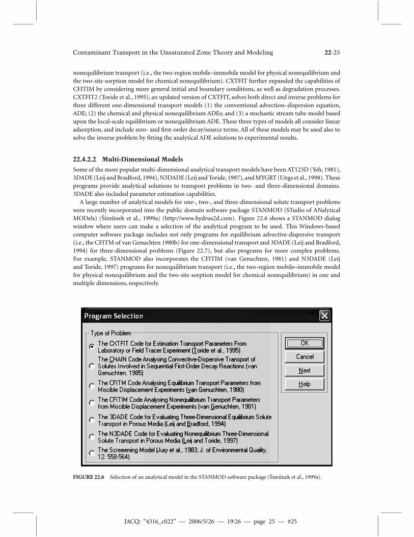
JACQ: “4316_c022” — 2006/5/26 — 19:26 — page 25 — #25


nonequilibrium transport (i.e., the two-region mobile–immobile model for physical nonequilibrium andthe two-site sorption model for chemical nonequilibrium). CXTFIT further expanded the capabilities ofCFITIM by considering more general initial and boundary conditions, as well as degradation processes.CXTFIT2 (Toride et al., 1995), an updated version of CXTFIT, solves both direct and inverse problems forthree different one-dimensional transport models (1) the conventional advection–dispersion equation,ADE; (2) the chemical and physical nonequilibrium ADEs; and (3) a stochastic stream tube model basedupon the local-scale equilibrium or nonequilibrium ADE. These three types of models all consider linearadsorption, and include zero- and first-order decay/source terms. All of these models may be used also tosolve the inverse problem by fitting the analytical ADE solutions to experimental results.

22.4.2.2 Multi-Dimensional Models

Some of the more popular multi-dimensional analytical transport models have been AT123D (Yeh, 1981),3DADE (Leij and Bradford, 1994), N3DADE (Leij and Toride, 1997), and MYGRT (Ungs et al., 1998). Theseprograms provide analytical solutions to transport problems in two- and three-dimensional domains.3DADE also included parameter estimation capabilities.

A large number of analytical models for one-, two-, and three-dimensional solute transport problemswere recently incorporated into the public domain software package STANMOD (STudio of ANalyticalMODels) (Šimunek et al., 1999a) (http://www.hydrus2d.com). Figure 22.6 shows a STANMOD dialogwindow where users can make a selection of the analytical program to be used. This Windows-basedcomputer software package includes not only programs for equilibrium advective-dispersive transport(i.e., the CFITM of van Genuchten 1980b) for one-dimensional transport and 3DADE (Leij and Bradford,1994) for three-dimensional problems (Figure 22.7), but also programs for more complex problems.For example, STANMOD also incorporates the CFITIM (van Genuchten, 1981) and N3DADE (Leijand Toride, 1997) programs for nonequilibrium transport (i.e., the two-region mobile–immobile modelfor physical nonequilibrium and the two-site sorption model for chemical nonequilibrium) in one andmultiple dimensions, respectively.

FIGURE 22.6 Selection of an analytical model in the STANMOD software package (Šimunek et al., 1999a).

JACQ: “4316_c022” — 2006/5/26 — 19:26 — page 26 — #26


FIGURE 22.7 Selection of the geometry of the transport domain for the 3DADE code (Leij and Bradford, 1994)within the STANMOD software package (Šimunek et al., 1999a).

Figure 22.7 shows a dialog window of STANMOD in which users can select the geometry of thetransport domain for use in the 3DADE program. STANMOD also includes CXTFIT2 (Toride et al.,1995) as discussed earlier, and the CHAIN code of van Genuchten (1985) for analyzing the advective–dispersive transport of up to four solutes involved in sequential first-order decay reactions. Examples ofthe latter are the migration of radionuclides in which the chain members form first-order decay reactions,and the simultaneous movement of various interacting nitrogen or organic chemicals. The latest versionof STANMOD also includes the screening model of Jury et al. (1983) for describing transport andvolatilization of soil-applied volatile organic chemicals.

An application of CFITIM within of the STANMOD program is demonstrated in Figure 22.8, whichshows measured and fitted breakthrough curves of a nonreactive (3H2O) solute for transport througha saturated Glendale clay loam soil. In this example, a tritiated water pulse of 3.102 pore volumes wasapplied to a 30 cm long column, with the breakthrough curve being determined from the effluent con-centrations. An analytical solution for two-region (mobile–immobile) physical nonequilibrium transport(van Genuchten, 1981) was used for the analysis. With the pore-water velocity known (v = 37.54 cm d−1)

and assuming that the retardation factor R for 3H2O was equal to one (no sorption or anion exclusion),only three parameters were optimized against the breakthrough curve, that is, the dispersion coefficientD (= 15.6 cm2 d−1), a dimensionless variable β (= 0.823) for partitioning the liquid phase in mobile andimmobile regions, and a dimensionless mass transfer coefficient ω (= 0.870).

An example application of the 3DADE program (Leij and Bradford, 1994) in the STANMOD packageis demonstrated in Figure 22.9, which shows calculated concentration contours for a transport problemin which solute is applied at a concentration C0 = 1, assuming a third-type boundary condition, to arectangular area of the soil surface (or within groundwater) of 15× 15 cm2. Other transport parameterswere as follows: v = 10 cm d−1, Dx = 100 and Dy = Dz = 10 cm2 d−1, and R = 1. Figure 22.9 showsconcentration contours in the xy-plane at t = 1 days, and z = 0.

JACQ: “4316_c022” — 2006/5/26 — 19:26 — page 27 — #27


00 2 4 6

0.2

0.4

0.6

0.8

1

1.2

8

Pore volumes [–]

Con

cent

ratio

n [–

]

Measured

Fitted

FIGURE 22.8 Breakthrough curve for nonreactive tritium transport as analyzed with the two-region physicalnonequilibrium program CXTFIT2 (Toride et al., 1995) within STANMOD (Šimunek et al., 1999a).

20

0

y

–20

0.0 0.2 0.4 0.6 0.8 1.0

0 x 30

FIGURE 22.9 Solute distribution in the xy-plane for continuous application at x = 0 and −7.5 < y < 7.5 cm after1 days, with v = 10 cm d−1, Dx = 100 and Dy = Dz = 10 cm2 d−1 as calculated with 3DADE (Leij and Bradford,1994) within STANMOD (Šimunek et al., 1999a).

22.5 Numerical Models

22.5.1 Numerical Approaches

While analytical and semi-analytical solutions are still popularly used for many relatively simple applic-ations, the ever-increasing power of personal computers, and the development of more accurate and

JACQ: “4316_c022” — 2006/5/26 — 19:26 — page 28 — #28


stable numerical solution techniques, have led to the much wider use of numerical models in recent years.Numerical methods are in general superior to analytical methods in terms of being able to solve muchmore practical problems (Šimunek, 2005). They allow users to design complicated geometries that reflectcomplex natural geologic and hydrologic conditions, control parameters in space and time, prescribemore realistic initial and boundary conditions, and permit the implementation of nonlinear constitutiverelationships. Numerical methods usually subdivide the time and spatial coordinates into smaller pieces,such as finite differences, finite elements, and finite volumes, and reformulate the continuous form ofgoverning partial differential equations in terms of a system of algebraic equations. To obtain solutionsat certain times, numerical methods generally require intermediate simulations (time-stepping) betweenthe initial condition and the points in time for which the solution is needed.

Reviews of the history of development of various numerical techniques used in vadose zone flow andtransport models are given by van Genuchten and Šimunek (1996) and Šimunek (2005). Here we willsummarize only the main principles behind some of the more popular techniques.

22.5.1.1 Finite Differences

The method of finite differences is generally very intuitive and relatively easy to implement. Time andspace are both divided into small increments �t and �z (or �x and �z) (Figure 22.10). Temporal andspatial derivatives in the governing equation are then replaced with finite differences (formally using Taylorseries expansions). For example, the standard advection–dispersion equation for steady-state water flow:

∂c

∂t= − ∂J

∂z= D

∂2c

∂z2− v

∂c

∂z(22.64)

can be approximated as follows using an explicit (forward-in-time) finite difference scheme:

cj+1i − c

ji

�t= − J

ji+1/2 − J

ji−1/2

�z= D

cji+1 − 2c

ji + c

ji−1

(�z)2− v

cji+1 − c

ji−1

2�z(22.65)

where subscripts refer to spatial discretization and superscript to temporal discretization (j and j+1 arefor the previous and actual time levels, respectively; see Figure 22.10), �t is the time step, and �z is thespatial step (assumed to be constant). Notice that this equation contains only one unknown variable (i.e.,

the concentration cj+1i at the new time level), which hence can be evaluated directly (explicitly) by solving

the equation.

zi+1 ci +1

ci ci

ci +1

ci – 1ci – 1

j +1

j +1

j +1

j

j

j

t i+1ti

zi –1

zi

z

t

∆t

∆z

∆zi

∆x

∆xi–1 ∆xi

∆z

∆zj

x

zj

z

∆zi–1

zj – 1

zj+1

∆zj – 1

xi –1

ci –1, j +1

ci–1, j

ci–1, j –1

ci, j

ci +1, j +1

ci+1, j

ci+1, j–1ci, j–1

ci, j +1

xi + 1xi(a) (b)

FIGURE 22.10 Examples of the spatial and temporal finite difference discretization of a one-dimensionalproblem (a), and the finite difference discretization of a two-dimensional domain (b).

JACQ: “4316_c022” — 2006/5/26 — 19:26 — page 29 — #29


By comparison, a fully implicit (backward-in-time) finite difference scheme can be written as follows:

cj+1i − c

ji

�t= − J

j+1i+1/2 − J

j+1i−1/2

�z= D

cj+1i+1 − 2c

j+1i + c

j+1i−1

(�z)2− v

cj+1i+1 − c

j+1i−1

2�z(22.66)

and an implicit (weighted) finite difference scheme as:

cj+1i − c

ji

�t=D

ε(cj+1i+1 − 2c

j+1i + c

j+1i−1 )+ (1− ε)(c j

i+1 − 2cji + c

ji−1)

(�z)2

− vε(c

j+1i+1 − c

j+1i−1 )+ (1− ε)(c j

i+1 − cji−1)

2�z(22.67)

where ε is a temporal weighting coefficient. Different finite-difference schemes results depending uponthe value of ε, that is, an explicit scheme when ε = 0, a Crank–Nicholson time-centered scheme whenε = 0.5, and a fully implicit scheme when ε = 1. Of these, the latter two cases lead to several unknownconcentrations in each equation at the new time level. Consequently, equations for all nodes of thetransport domain need to be assembled into an algebraic system of linear equations to produce a matrixequation of the form

[P]j+1{c}j+1 = {F} (22.68)

in which [P] is a tridiagonal matrix [P] given by:

[P] =

∣∣∣∣∣∣∣∣∣∣∣∣∣∣∣∣

d1 e1 0 0b2 d2 e2 0 00 b3 d3 e3 0 0

......

...0 0 bN−2 dN−2 eN−2 00 0 bN−1 dN−1 eN−1

0 0 bN dN

∣∣∣∣∣∣∣∣∣∣∣∣∣∣∣∣

(22.69)

Equation 22.69 is subsequently solved using a matrix equation solver to yield the concentrations at thenew time level.

The problem becomes more complex for problems involving transient flow. In that case one mustfirst obtain estimates of the water contents and fluxes at the new time level using a numerical solutionof the Richards equation. These water contents and fluxes are subsequently used for assembling thematrix equations for solute transport. While finite differences are relatively straightforward to implementfor many transport problems, one major disadvantage is that this method cannot be easily applied torelatively complicated (irregular) transport domains in two and three dimensions.

22.5.1.2 Finite Elements

Finite element methods can be implemented in very much the same way as finite differences for one-, two-,and three-dimensional problems. A major advantage of the finite elements is that they are much easierused to discretize complex two- and three-dimensional transport domains (Figure 22.11). As an example,Figure 22.11 shows triangular unstructured finite element grids for a regular rectangular and an irregulardomain as generated with the automated MeshGen2D mesh generator of HYDRUS-2D (Šimunek et al.,1999b). Note that even though the figure on the right (Figure 22.11) has an irregular soil surface, as well asa tile drain within the transport domain, MeshGen2D could easily discretize/accommodate this transportdomain using an unstructured triangular finite element mesh.

The finite element method assumes that the dependent variable in the advection–dispersion equation(e.g., the concentration function c(x , t ) in (22.64)) can be approximated by a finite series c ′(x , t ) of the

JACQ: “4316_c022” — 2006/5/26 — 19:26 — page 30 — #30


Z

X

(a) (b)

FIGURE 22.11 Examples of the triangular finite element grids for regular (a) and irregular (b) two-dimensionaltransport domains.

i -1 i i +1

�1 �2

∆xi

x

c

ci–1ci+1

1

x

ci

i – 1

1

i + 1 xi

(a)

(b)

FIGURE 22.12 Example of one-dimensional linear basis functions (a) and their use to approximate solution c(x , t )of the advection–dispersion equation (b).

form (Figure 22.12b):

c ′(x , t ) =N∑

m=1

φm(x)cm(t ) (22.70)

where φm are the selected linear basis functions that fulfill the condition φm(xn) = δnm , δnm is Kroneckerdelta ( δnm = 1 for m = n, and δnm = 0 for m �= n), cm are the unknown time-dependent coefficientswhich represent solutions of (22.64) at the finite element nodal points, and N is the total number of nodalpoints. For example, for the one-dimensional finite element xi < x < xi+1, linear basis functions have

JACQ: “4316_c022” — 2006/5/26 — 19:26 — page 31 — #31


the following form (Figure 22.12a):

φ1 = 1− x − xi

�x

φ2 = x − xi

�x

xi ≤ x ≤ xi+1 (22.71)

where �x (= xi+1 − xi) is the size of a finite element [L], that is, the distance between two neighboringnodal points. The approximate solution c ′(x , t ) converges to the correct solution c(x , t ) as the number ofbasis functions N increases.

Application of the Galerkin method, which postulates that the differential operator associated with thetransport equation is orthogonal to each of the N basis functions (e.g., Pinder and Gray, 1977), leads tothe following system of N time-dependent differential equations with N unknown values cn(t ):

L∫0

(−∂c

∂t− D

∂2c

∂x2− v

∂c

∂x

)φn dx = 0 (22.72)

where φn are the selected linear weighting functions that can be the same as the basis functions φm.Integrating by parts the terms containing the spatial derivatives to remove the second-order derivatives,and substituting (22.70) for c(x , t ) leads to the following equation:

∑e

Le∫0

(−∂cm

∂tφm

)φn dx −

∑e

Le∫0

(Dcm

∂φm

∂x− vcmφm

)∂φn

∂xdx − qsLφn(L)+ qs0φn(0) = 0

(22.73)

where qs0 and qsL are solute fluxes across the left and right boundaries, respectively; e is the element index,Le is the size of an element e, and L is the size of the transport domain (length of the soil profile). Theintegrals in Equation 22.73 can be evaluated either numerically or analytically, depending upon the typeof invoked basis and weighting functions ( φm and φn , respectively). The equation can be rewritten inmatrix form similarly as (Equation 22.68) and then solved using a matrix equation solver. For a detailedderivation of the matrix equation we refer to standard finite element textbooks (e.g., Pinder and Gray, 1977;Zienkiewicz, 1977; Huyakorn and Pinder, 1983) or manuals of some of the models (e.g., the HYDRUSmodels by Šimunek et al., 1998a,b).

22.5.1.3 Stability and Oscillations

Numerical solutions of the transport equation often exhibit oscillatory behavior and/or excessive numer-ical dispersion near relatively sharp concentration fronts (Huyakorn and Pinder, 1983; Šimunek et al.,1998a). These problems can be especially serious for advection-dominated transport characterized bysmall dispersivities. One way to partially circumvent numerical oscillations is to use upstream weighingin which case the flux term of Equation 22.64 is not weighted using regular linear basis functions φn ,but instead with nonlinear quadratic functions φu

n . Undesired oscillations can often be prevented also byselecting an appropriate combination of the space and time discretizations. Two dimensionless numbersmay be used to characterize the discretizations in space and time. One of these is the grid Peclet num-ber, Pee, which defines the predominant type of solute transport (notably the ratio of the advective anddispersive transport terms) in relation to coarseness of the finite element grid:

Pee = v�x

D(22.74)

JACQ: “4316_c022” — 2006/5/26 — 19:26 — page 32 — #32


where�x is the characteristic length of a finite element [L]. The Peclet number increases when the advect-ive part of the transport equation dominates the dispersive part (i.e., when a relatively steep concentrationfront is present). To achieve acceptable numerical results, the spatial discretization must be kept relativelyfine to maintain a low Peclet number. Numerical oscillations can be virtually eliminated when the localPeclet numbers do not exceed about 5. However, acceptably small oscillations may be obtained withlocal Peclet numbers as high as 10 (Huyakorn and Pinder, 1983). Undesired oscillations for higher Pecletnumbers can be effectively eliminated by using upstream weighing.

A second dimensionless number, the Courant number, Cre, may be used to characterize the relativeextent of numerical oscillations in the numerical solution. The Courant number is associated with thetime discretization,�t [T], as follows:

Cre = v�t

�x(22.75)

Given a certain spatial discretization, the time step must be selected such that the Courant number remainsless than or equal to 1.

Perrochet and Berod (1993) developed a criterion for minimizing or eliminating numerical oscillationsthat is based on the product of the Peclet and Courant numbers:

Pe · Cr ≤ ωs (=2) (22.76)

where ωs is the performance index [−]. This criterion indicates that advection-dominated transportproblems having large Pe numbers can be safely simulated provided Cr is reduced according to (22.76)(Perrochet and Berod, 1993). When small oscillations in the solution can be tolerated,ωs can be increasedto about 5 or 10.

22.5.2 Existing Models

22.5.2.1 Single-Species Solute Transport Models

A large number of numerical models are now available for evaluating variably saturated water flow andsolute transport processes in the subsurface. Some of these models are in the public domain, such asMACRO (Jarvis, 1994), SWAP (van Dam et al., 1997), UNSATH (Fayer, 2000), VS2DI (Healy, 1990), andHYDRUS-1D (Šimunek et al., 1998a, 2005), while others are in the commercial domain, such as HYDRUS-2D (Šimunek et al., 1999b) and MODFLOW-SURFACT (HydroGeoLogic, 1996). These models varywidely in terms of their complexity, sophistication, and ease of use. Although some models are still beingrun under the DOS operating system, with associated difficulties of preparing input files and interpretingtabulated outputs, many others, especially those in the commercial domain, are supported by sophisticatedgraphics-based interfaces that greatly simplify their use (Šimunek et al., 1998a; 1999b). Several studieshave recently reviewed and compared various numerical models for vadose zone applications (e.g., Wilsonet al., 1999; Scanlon et al., 2002; MDH Engineered Solutions Corp., 2003; Vanderborght et al., 2005). Thesestudies typically evaluated comparable precision, speed, and ease of use of the codes involved.

While many of the early numerical zone models were developed mostly for agricultural applications(e.g., optimizing soil moisture conditions for crop production), this focus has increasingly shifted toenvironmental research, with the primary concern now being the subsurface fate and transport of vari-ous agricultural and other contaminants, such as radionuclides, hydrocarbons, fumigants, pesticides,nutrients, pathogens, pharmaceuticals, viruses, bacteria, colloids, and/or toxic trace elements. The earliermodels solved the governing flow and transport equations for relatively simplified system-independentboundary conditions (i.e., specified pressure heads or fluxes, and free drainage). Models developed recentlycan cope with much more complex system-dependent boundary conditions evaluating surface flow andenergy balances and accounting for the simultaneous movement of water, vapor, and heat. Examples areDAISY (Hansen et al., 1990), TOUGH2 (Pruess, 1991), SHAW (Flerchinger et al., 1996), SWAP (van Damet al., 1997), HYDRUS-1D (Šimunek et al., 1998a, 2005), UNSATH (Fayer, 2000), and COUP (Jansson

JACQ: “4316_c022” — 2006/5/26 — 19:26 — page 33 — #33


and Karlberg, 2001). Several models now also account for the extremely nonlinear processes associatedwith the freezing and thawing cycle (e.g., DAISY, SHAW, and COUP).

Models have recently also become increasingly sophisticated in terms of the type and complexityof solute transport processes that can be simulated. Transport models are no longer being limited tosolutes undergoing relatively simple chemical reactions such as linear sorption and first-order decay,but now consider also a variety of nonlinear sorption and exchange processes, physical and chemicalnonequilibrium transport, volatilization, gas diffusion, colloid attachment/ detachment, decay chainreactions, and many other processes (e.g., the HYDRUS-1D and -2D codes of Šimunek et al., 1999b,2005, or MODFLOW-SURFACT of HydroGeoLogic, Inc., 1996). For example, the general formulation ofthe transport equations in the HYDRUS codes permit simulations of not only non-adsorbing or linearlysorbing chemicals, but also of a variety of other contaminants, such a viruses (Schijven and Šimunek,2001), colloids (Bradford et al., 2002), cadmium (Seuntjens et al., 2001), and hormones (Casey et al.,2003, 2004), or chemicals involved in the sequential biodegradation of chlorinated aliphatic hydrocarbons(Schaerlaekens et al., 1999; Casey and Šimunek, 2001).

Much effort has recently been directed also toward improving models for purposes of simulatingnonequilibrium and/or preferential flow. Examples of this are the TOUGH codes (Pruess, 1991, 2004),MACRO (Jarvis, 1994), and HYDRUS-1D (Šimunek et al., 2003, 2005). These models typically assume thepresence of dual-porosity and dual-permeability regions, with different fluxes possible in the two regions.As discussed in detail in Section 22.2b, dual-porosity, mobile–immobile water flow models result when theRichards or kinematic wave equations are used for flow in the fractures, and immobile water is assumedto exist in the matrix, whereas dual-permeability models assume that water is mobile in both the matrixand fracture domains, while invoking terms accounting for the exchange of water and solutes betweenthe two regions. Example applications of these dual-porosity and dual-permeability models are given byŠimunek et al. (2001), Haws et al. (2005), Köhne et al. (2004b, 2005), and Pot et al. (2005), among manyothers.

As an example of available vadose zone flow and transport models, we discuss here in somewhat greaterdetail the HYDRUS software packages of Šimunek et al. (1999b, 2005) and the MODFLOW-SURFACTmodel developed by HydroGeoLogic (1996).

22.5.2.1.1 The HYDRUS Software PackagesHYDRUS-1D (Šimunek et al., 2005) and HYDRUS-2D (Šimunek et al., 1999b) are software packages(www.hydrus2d.com) that simulate the one- and two-dimensional movement of water, heat, and multiplesolutes in variably saturated media, respectively. Both programs use finite elements to numerically solve theRichards equation for saturatedunsaturated water flow and Fickian-based advectiondispersion equationsfor both heat and solute transport. The flow equation includes a sink term to account for water uptakeby plant roots as a function of both water and salinity stress. The flow equation may also considerdual-porosity-type flow with a fraction of water content being mobile, and fraction immobile. The heattransport equation considers conduction as well as advection with flowing water. The solute transportequations assume advective-dispersive transport in the liquid phase, and diffusion in the gaseous phase.The transport equations also include provisions for nonlinear and/or nonequilibrium reactions betweenthe solid and liquid phases, linear equilibrium reactions between the liquid and gaseous phases, zeroorderproduction, and two firstorder degradation reactions: one which is independent of other solutes, andone which provides the coupling between solutes involved in the sequential first-order decay reactions.In addition, physical nonequilibrium solute transport can be accounted for by assuming a two-region,dual-porosity type formulation which partitions the liquid phase into mobile and immobile regions.Alternatively, the transport equations include provisions for kinetic attachment/detachment of solute tothe solid phase and thus can be used to simulate the transport of viruses, colloids, or bacteria (Schijvenand Šimunek, 2002; Bradford et al., 2003).

Both programs may be used to analyze water and solute movement in unsaturated, partially saturated,or fully saturated media. The flow region itself may consist of nonuniform (layered) soils. HYDRUS-2Dadditionally can handle flow regions delineated by irregular boundaries. The flow region itself may be

JACQ: “4316_c022” — 2006/5/26 — 19:26 — page 34 — #34


composed of nonuniform soils having an arbitrary degree of local anisotropy. Flow and transport can occurin the vertical plane, the horizontal plane, or in a three-dimensional region exhibiting radial symmetryabout the vertical axis. The unsaturated soil hydraulic properties (the constitutive relationships) can bedescribed using van Genuchten (1980a), Brooks and Corey (1964), Kosugi (1996), and Durner (1994)type analytical functions, or modified van Genuchten type functions that produce a better description ofthe hydraulic properties near saturation. HYDRUS-1D incorporates hysteresis by assuming that dryingscanning curves are scaled from the main drying curve, and wetting scanning curves from the main wettingcurve. Root growth is simulated by means of a logistic growth function, while root water uptake can besimulated as a function of both water and salinity stress.

The HYDRUS-1D software package additionally includes modules for simulating carbon dioxide andmajor ion solute movement (Šimunek et al., 1996). Diffusion in both the liquid and gas phases and advec-tion in the liquid phase are considered as the main CO2 transport mechanisms (Šimunek and Suarez,1993). The major variables of the chemical system are Ca, Mg, Na, K, SO4, Cl, NO3, H4SiO4, alkalin-ity, and CO2(Šimunek and Suarez, 1994; Šimunek et al., 1996). The model accounts for equilibriumchemical reactions between these components such as complexation, cation exchange and precipitation-dissolution. For the precipitation-dissolution of calcite and dissolution of dolomite, either equilibriumor multicomponent kinetic expressions are used, involving both forward and back reactions. Otherdissolution-precipitation reactions considered include gypsum, hydromagnesite, nesquehonite, and sepi-olite. Since the ionic strength of soil solutions can vary considerably with time and space and often reachhigh values, both modified Debye–Hückel and Pitzer expressions were incorporated into the model asoptions to calculate single ion activities.

In addition, both HYDRUS programs implement a Marquardt-Levenberg type parameter estimationtechnique (Marquardt, 1963; Šimunek and Hopmans, 2002) for inverse estimation of soil hydraulic(Šimunek et al., 1998b,c; Hopmans et al., 2002) and/or solute transport and reaction (Šimunek et al.,2002) parameters from measured transient or steady-state flow and/or transport data.

The HYDRUS packages use a Microsoft Windows based Graphics User Interface (GUI) to manage theinput data required to run the program, as well as for nodal discretization and editing, parameter allocation,problem execution, and visualization of results. All spatially distributed parameters, such as those forvarious soil horizons, the root water uptake distribution, and the initial conditions for water, heat andsolute movement, are specified in a graphical environment. HYDRUS-2D includes the MeshGen2D meshgenerator, specifically designed for variably-saturated subsurface flow transport problems, for definingmore general domain geometries, and for discretizing the transport domain into an unstructured finiteelement mesh. The program offers graphs of the distributions of the pressure head, water content, waterand solute fluxes, root water uptake, temperature, and solute concentrations in the soil profile at pre-selected times. Also included is a small catalog of unsaturated soil hydraulic properties (Carsel and Parish,1988), as well as pedotransfer functions based on neural networks (Schaap et al., 2001). Many differentapplications of both software packages were referenced throughout this book chapter.

22.5.2.1.2 MODFLOW-SURFACTMODFLOW-SURFACT (HydroGeoLogic, 1996) is a fully integrated flow and transport code, based onthe MODFLOW groundwater modeling software package of the U.S. Geological Survey (McDonald andHarbaugh, 1988). While MODFLOW (see detailed discussion in Chapter 20) deals only with fully saturatedgroundwater flow, MODFLOW-SURFACT expands the applicability of the code to unsaturated domains.MODFLOW-SURFACT includes new flow packages that enhance schemes for performing unconfinedsimulations to rigorously model desaturation and resaturation of aquifers. It provides an option fordiscretizing the domain using an axi-symmetric geometry for efficient simulation of pumping tests,recovery tests, etc. In addition to normally allowed external stresses in MODFLOW (i.e., constant head,constant flux, areal recharge, evapotranspiration, drains, and streams), MODFLOW-SURFACT provides arigorous well withdrawal package, unconfined recharge boundary conditions, and seepage face boundaryconditions. Additionally, MODFLOW-SURFACT also includes options for adaptive time-stepping and

JACQ: “4316_c022” — 2006/5/26 — 19:26 — page 35 — #35


output control procedures, and a new solution package based on the preconditioned conjugate gradientmethod.

MODFLOW-SURFACT includes new Analysis of Contaminant Transport (ACT) modules that allowsimulations of single-species and multi-component contaminant transport. The program can handle up to5 chemical species, which may undergo linear or nonlinear retardation, first-order decay and biochemicaldegradation, as well as generate transformation products. MODFLOW-SURFACT also permits masspartitioning of a single or multicomponent contaminant with diffusive mass movement in the inactivephase, and mass partitioning of a single or multicomponent contaminant from a depleting immobileNAPL phase with advective and dispersive transport in the active phase and diffusive transport in theinactive phase.

22.5.2.2 Geochemical Transport Models

Significant efforts have recently been recently carried out also in coupling physical flow and transportmodels with geochemical models to simulate ever more complex reactions, such as surface complexation,precipitation/dissolution, cation exchange, and biological reactions. Recent reviews of the developmentof hydrogeochemical transport models involving reactive multiple components are given by Mangold andTsang (1991), Lichtner (1996) and Steefel and MacQuarrie (1996), Šimunek and Valocchi (2002), and Belland Binning (2004). Most modeling efforts involving multicomponent transport have thus far focused onthe saturated zone, where changes in the water flow velocity, temperature and pH are often much moregradual and hence less important than in the unsaturated zone. Consequently, most multicomponenttransport models assumed one- or two-dimensional steady-state saturated water flow with a fixed value ofthe flow velocity, temperature and pH. Only recently have several multicomponent transport models beenpublished which also consider variably saturated flow; these include DYNAMIX (Liu and Narasimhan,1989), HYDROGEOCHEM (Yeh and Tripathi, 1990), TOUGH-REACT (Pruess, 1991), UNSATCHEM(Šimunek and Suarez, 1994; Šimunek et al., 1996, 1997), FEHM (Zyvoloski et al., 1997), MULTIFLO(Lichtner and Seth, 1996), OS3D/GIMRT (Steefel and Yabusaki, 1996), HYDROBIOGEOCHEM (Yehet al., 1998), FLOTRAN (Lichtner, 2000), MIN3P (Mayer et al., 2002), HP1 (Jacques et al., 2002; Jacquesand Šimunek, 2005), and HYDRUS-1D (Šimunek et al., 2005).

Geochemical models can be divided into two major groups: those with specific chemistry and generalmodels (Šimunek and Valocchi, 2002). Models with specific chemistry are limited in the number of speciesthey can handle, while their application is restricted to problems having a prescribed chemical system.They are, however, much easier to use and computationally can be much more efficient than generalmodels. Typical examples of models with specified chemistry are those simulating the transport of majorions, such as LEACHM (Wagenet and Hutson, 1987), UNSATCHEM (Šimunek and Suarez, 1994; Šimuneket al., 1996), and HYDRUS-1D (Šimunek et al., 2005). Models with generalized chemistry (DYNAMIX,HYDROGEOCHEM, MULTIFLO, FLOTRAN, OS3D/GIMRT, and HP1, all referenced above) provideusers with much more freedom in designing a particular chemical system; possible applications of thesemodels are also much wider.

22.5.2.2.1 HP1HYDRUS-1D was recently coupled with the PHREEQC geochemical code (Parkhurst and Appelo, 1999)to create a new comprehensive simulation tool, HP1 (acronym for HYDRUS1D-PHREEQC) (Jacqueset al., 2003; Jacques and Šimunek, 2005). The combined code contains modules simulating (1) transientwater flow in variably saturated media, (2) the transport of multiple components, (3) mixed equilib-rium/kinetic biogeochemical reactions, and (4) heat transport. HP1 is a significant expansion of theindividual HYDRUS-1D and PHREEQC programs by preserving most of their original features andcapabilities. The code still uses the Richards equation for simulating variably saturated water flow andadvection–dispersion type equations for heat and solute transport. However, the program can now sim-ulate also a broad range of low-temperature biogeochemical reactions in water, the vadose zone and inground water systems, including interactions with minerals, gases, exchangers, and sorption surfaces,based on thermodynamic equilibrium, kinetics, or mixed equilibrium-kinetic reactions.

JACQ: “4316_c022” — 2006/5/26 — 19:26 — page 36 — #36


0.0008

0.0006

0.0004

0.0002

0

0.012

0.01

0.008

0.006

0.004

0.002

00 3 6 9 12 15 0 3 6 9 12 15

Time [days]

(a) (b)

Time [days]

Na

Ca

Cd

Pb

ZnCl

Al

Con

cent

ratio

ns [m

ol/L

]

Con

cent

ratio

ns [m

ol/L

]

FIGURE 22.13 Major ions (a) and heavy metals (Zn, Pb, and Cd) (b) concentrations in the effluent of an 8-cm soillong column.

Jacques et al. (2003) and Jacques and Šimunek (2005) demonstrated the versatility of the HP1 modelon several examples such as (a) the transport of heavy metals (Zn2+, Pb2+, and Cd2+) subject to mul-tiple cation exchange reactions, (b) transport with mineral dissolution of amorphous SiO2 and gibbsite(Al(OH)3), (c) heavy metal transport in a medium with a pH-dependent cation exchange complex,(d) infiltration of a hyperalkaline solution in a clay sample (this example considers kinetic precipitation–dissolution of kaolinite, illite, quartz, calcite, dolomite, gypsum, hydrotalcite, and sepiolite), (e) long-termtransient flow and transport of major cations (Na+, K+, Ca2+, and Mg2+) and heavy metals (Cd2+, Zn2+,and Pb2+) in a soil profile, (f) cadmium leaching in acid sandy soils, (g) radionuclide transport (U andits aqueous complexes), and (h) the fate and subsurface transport of explosives (TNT and its daughterproducts 2ADNT, 4ADNT, and TAT) (Šimunek et al., 2006).

22.5.2.2.2 Leaching of Heavy Metals from a Soil ColumnAs an example application of HP1, Figure 22.13 shows calculated effluent concentrations of heavy metals(Zn2+, Pb2+, and Cd2+) leached from an 8-cm long soil column having an initial solution as defined inTable 22.2, and with its ion-exchange complex in equilibrium with this solution. Heavy metals initiallypresent in the soil column are leached from the exchange complex by major ions (Ca2+, Mg2+, and Al3+).Water was applied to the top of the column at a steady flow rate of 2 cm day−1 and having a chemicalcomposition as given in Table 22.2. Details are given by Jacques and Šimunek (2005).

22.6 Concluding Remarks

This chapter demonstrates the abundance of models and modeling approaches that are currently availablefor simulating variably saturated water flow and contaminant transport at various levels of approximationand for different applications. Models range from relatively simple analytical approaches for analyzingsolute transport problems during one-dimensional steady-state flow, to sophisticated numerical modelsfor addressing multi-dimensional variably saturated flow and contaminant transport problems at the fieldscale.

One may expect that unsaturated zone flow and transport models will be used increasingly as tools fordeveloping cost-effective, yet technically sound strategies for resource management and pollution remedi-ation and prevention. Improved understanding of the key underlying processes, continued advances innumerical methods, and the introduction of more and more powerful computers make such simula-tions increasingly practical for many field-scale problems. For example, models can be helpful tools fordesigning, testing and implementing soil, water and crop management practices that minimize soil andwater pollution. Models are equally needed for designing or remediating industrial waste disposal sites

JACQ: “4316_c022” — 2006/5/26 — 19:26 — page 37 — #37


TABLE 22.2 Chemical Components (mmol/L) and Species Considered, and ElementalCompositions of Initial and Boundary Solutions Used in the Column Simulation. X Refersto Ion Exchanger

Solutions

Components Species Boundary Initial

Al Al3+, Al(OH)2+, Al(OH)+2 , Al(OH)03, Al(OH)−4 0.1 0.5

Br Br− 3.7 11.9Cl Cl− (and Cd, Pb, and Zn-species, see below) 10 0Ca Ca2+, Ca(OH)+ 5 0K K+, KOH0 0 2Na Na+, NaOH0 0 6Mg Mg2+, Mg(OH)+ 1 0.75

Cd Cd2+, Cd(OH)+, Cd(OH)02, Cd(OH)−3 , Cd(OH)2−

4 , CdCl+,CdCl2, CdCl−3 0 0.9

Pb Pb2+, Pb(OH)+, Pb(OH)02, Pb(OH)−3 , Pb(OH)2−

4 , PbCl+, PbCl02,

PbCl−3 , PbCl2−4 0 0.1

Zn Zn2+, Zn(OH)+, Zn(OH)02, Zn(OH)−3 , Zn(OH)2−

4 , ZnCl+, ZnCl02,

ZnCl−3 , ZnCl2−4 0 0.25X AlX3, AlOHX2, CaX2, CdX2, KX, NaX, MgX2, PbX2, ZnX2 (mmol) NA 11

and landfills, for predicting contaminant transport from mining wastes, or for long-term stewardship ofnuclear waste repositories. The main challenge is to make the models as realistic as possible for the variousapplications.

Continued progress in subsurface flow and transport modeling requires equal advances in both numer-ical techniques as well as the underlying science. Addressing preferential flow phenomena, and the relatedproblems of subsurface heterogeneity, including the stochastic nature of boundary conditions (precip-itation and/or evapotranspiration), will continute to pose formidable challenges. The same is true forimproving multicomponent geochemical transport modeling for the vadose zone. For example, numericalalgorithms and databases for multicomponent transport models must be extended to higher temperaturesand ionic strengths, complex contaminant mixtures (including especially mixed organic and inorganicwastes), multiphase flow, redox disequilibria for low-temperature systems, and coupled physico-chemicalsystems to account for possible changes in the soil water retention and hydraulic conductivity functions.Better integration is also needed between variably satuarted subsurface and existing larger-scale surfacenumerical models, which in turn requires further research on such issues as spatial and temporal scalingof hydrological, chemical and biological processes and properties, linking constitutive (soil hydraulic)relationships to measurements scales, preferential flow, and issues of parameter and model uncertainty.

Many science questions related to colloid and colloid-facilitated transport are also still largely unre-solved. This is an area of research where our understanding lags far behind current numerical capabilities.Much work is needed to better understand the processes of filtration, straining, size exclusion, colloid–colloid interactions, mobilization of colloids and microorganisms; accumulation at air–water interfaces,interactions between microorganisms and contaminants (including biodegradation), the effects of bothphysical factors (water content, flow velocity, textural interfaces) and chemical processes (ionic strength,solution composition, pH) on colloid retention and mobilization, and modeling colloid-facilitatedtransport during conditions of transient flow.

Also, to the best of our knowledge, no models are currentely available that consider all the variousprocesses simultaneously and in their full complexity, including their mutual interactions. That is, nomodels exist that consider transient preferential flow and transport in structured soils or fractured rocks,while simultaneously considering complex biogeochemical reactions between contaminants, organic andinorganic colloids and/or organic complexes, and solid and air phases of a soil, including widely vary-ing rates of these various reactions. Further integration of the different types of numerical models is

JACQ: “4316_c022” — 2006/5/26 — 19:26 — page 38 — #38


needed to address practical problems of contaminant transport (trace elements, radionuclides, organiccontaminants) in complex vadose zone environments.

References

Abriola, L.M., Pennell, K.D., Weber, Jr., W.J. Lang, J.R. and Wilkins, M.D., Persistence and interphasemass transfer of organic contaminants in the unsaturated zone: Experimental observations andmathematical modeling. In J.Y. Parlange and J.W. Hopmans (Eds.) Vadose Zone Hydrology: CuttingAcross Disciplines. Oxford University Press, New York, pp. 210–234, 1999.

Adamczyk, Z., Siwek, B., Zembala, M. and Belouschek, P., Kinetics of localized adsorption of colloidparticles. Adv. Coll. Interf. Sci., 48, 151–280, 1994.

Ahuja, L.R. and Hebson, C., Root Zone Water Quality Model. GPSR Tech. Rep. No. 2, USDA, ARS, FortCollins, CO, 1992.

Anderson, M.P., Movement of contaminants in groundwater: Groundwater transport–advection anddispersion. In Groundwater Contamination, Studies in Geophysics, National Academy Press,Washington, D.C. pp. 37–45, 1984.

Appelo, C.A.J. and Postma, D., Geochemistry, Groundwater and Pollution. A. A. Balkema. Rotterdam, 1993.Bache, B.W. and Williams, E.G., A phosphate sorption index for soils. J. Soil Sci. 27, 289–296, 1971.Barry, D.A., Modelling contaminant transport in the subsurface: theory and computer programs. In

H. Ghadiri and C.W. Rose (Eds.), Modelling Chemical Transport in Soil: Natural and AppliedContaminants, Lewis Publishers, Chelsea, MI, pp. 105–144, 1992.

Bateman, H., The solution of a system of differential equations occurring in the theory of radioactivetransformation. Proc. Cambridge Philos. Soc., 15 (pt V) 423–427, 1910.

Bear, J., Dynamics of Fluids in Porous Media, Elsevier Science, New York, 1972.Bell, L.S.J. and Binning, P.J., A split operator approach to reactive transport with the forward particle

tracking Eulerian–Lagrangian localized adjoint method. Adv. Water Resour. 27, 323–334, 2004.Bethke, C. M., Geochemical Reaction Modeling — Concepts and Applications. Oxford University Press,

New York, p. 397, 1996.Biggar, J.W. and Nielsen, D.R., Miscible displacement and leaching phenomena. Agronomy 11, 254–274,

1967.Bradford, S.A., Yates, S.R., Bettahar, M. and Šimunek, J., Physical factors affecting the transport and fate of

colloids in saturated porous media. Water Resour. Res. 38, 1327, doi:10.1029/2002WR001340, 2002.Bradford, S. A., Šimunek, J., Bettahar, M., van Genuchten, M. Th. and Yates, S. R., Modeling colloid

attachment, straining, and exclusion in saturated porous media. Environ. Sci. Technol., 37, 2242–2250, 2003.

Bradford, S. A., Bettahar, M., Šimunek, J. and van Genuchten, M. Th., Straining and attachment of colloidsin physically heterogeneous porous media. Vadose Zone J. 3, 384–394, 2004.

Bresler, E. and Dagan G., Solute dispersion in unsaturated heterogeneous soil at field scale: I Applications.Soil Sci. Soc. Am. J. 43, 467–472, 1979.

Brooks, R.H. and Corey, A. T., Hydraulic properties of porous media. Hydrol. Paper No. 3, Colorado StateUniv., Fort Collins, CO, 1964.

Brusseau, M.L., Nonideal transport of reactive solutes in porous media; Cutting across history anddisciplines. In Parlange, M.B. and Hopmans, J.W. (Eds.), Vadose Zone Hydrology: Cutting AcrossDisciplines, Oxford University Press, New York, pp. 130–154, 1999.

Carsel, R.F. and Parrish, R. S., Developing joint probability distributions of soil water retentioncharacteristics. Water Resour. Res. 24, 755–769, 1988.

Casey, F.X.M. and Šimunek, J., Inverse analyses of the transport of chlorinated hydrocarbons subject tosequential transformation reactions. J. Environ. Qual., 30, 1354–1360, 2001.

Casey, F.X.M., Larsen, G.L., Hakk, H. and Šimunek, J., Fate and transport of 17β-Estradiol in soil-watersystems. Environ. Sci. Technol. 37, 2400–2409, 2003.

JACQ: “4316_c022” — 2006/5/26 — 19:26 — page 39 — #39


Casey, F.X.M., Larsen, G.L., Hakk, H. and Šimunek, J., Fate and transport of testosterone in agriculturallysignificant soils. Environ. Sci. Technol. 38, 790–798, 2004.

Corapcioglu, M.Y. and Jiang, S., Colloid-facilitated ground-water contaminant transport. Water Resour.Res. 29, 2215–2226, 1993.

Corapcioglu, M.Y. and Kim, S., Modeling facilitated contaminant transport by mobile bacteria. WaterResour. Res. 31, 2639–2644, 1995.

AQ: Please updateCotta et al.

Cotta, R.M., Goldstein, R., Heilbron, P.F.L. and Ungs, M.J. (Eds.), Hybrid Methods in Environ-mental Transport Phenomena, Center for Analysis and Simulation in Environmental Engineering,POLI/COPPE, Federal University of Rio de Janeiro, Brazil, 2005 (in press).

Dagan G. and E. Bresler, Solute dispersion in unsaturated heterogeneous soil at field scale: I Theory. SoilSci. Soc. Am. J. 43, 461–467, 1979.

Dagan G., Flow and Transport in Porous Formations, Springer-Verlag, Berlin, 1989.Durner, W., Hydraulic conductivity estimation for soils with heterogeneous pore structure. Water Resour.

Res. 32, 211–223, 1994.Fayer, M.J., UNSAT-H Version 3.0: Unsaturated Soil Water and Heat Flow Model. Theory, User Manual,

and Examples. Pacific Northwest National Laboratory 13249, 2000.Fitter, A.H. and Sutton, S.D., The use of the Freundlich isotherm for soil phosphate sorption data. J. Soil

Sci. 26, 241–246, 1975.Flerchinger, G.N., Hanson, C.L. and Wight, J.R., Modeling evapotranspiration and surface energy budgets

across a watershed. Water Resour. Res. 32, 2539–2548, 1996.Flury, M., Fluhler, H., Jury, W. and Leuenberger, J., Susceptibility of soils to preferential flow of water:

a field study. Water Resour. Res. 30, 1945–1954, 1994.Freundlich, H., Kapillarchemie; eine Darstellung der Chemie der Kolloide und verwandter Gebiete,

Akademische Verlagsgellschaft, Leipzig, Germany, 1909.Gelhar, L.W., Mantaglou, A., Welty, C. and Rehfeldt, K.R., A review of Field Scale Physical Solute Transport

Processes in Unsaturated and Saturated Porous Media, EPRI Topicl Report EA-4190, Electric PowerResearch Institute, Palo Alto, CA, 1985.

Gerke, H.H. and van Genuchten, M.Th., A dual-porosity model for simulating the preferential movementof water and solutes in structured porous media. Water Resour. Res. 29, 305–319, 1993a.

Gerke, H.H. and van Genuchten, M.Th., Evaluation of a first-order water transfer term for variablysaturated dual-porosity flow models. Water Resour. Res. 29, 1225–1238, 1993b.

Gerke, H.H. and van Genuchten, M.Th., Macroscopic representation of structural geometry for simulatingwater and solute movement in dual-porosity media. Adv. Water Resour. 19, 343–357, 1996.

Germann, P.F., Kinematic wave approach to infiltration and drainage into and from soil macropores.Trans. ASAE 28, 745–749, 1985.

Germann, P.F. and Beven, K., Kinematic wave approximation to infiltration into soils with sorbingmacropores. Water Resour. Res. 21, 990–996, 1985.

Glotfelty, D.E. and Schomburg, C.J., Volatilization of pesticides. In B.L. Sawhney and K. Brown (Eds.),Reactions and Movement of Organic Chemicals in Soils, Special Publ. No. 22, Soil Science Society ofAmerica, Madison, WI, pp. 181–208, 1989.

Grolimund, D., Borkovec, M., Barmettler, K. and Sticher, H., Colloid-facilitated transport of stronglysorbing contaminants in natural porous media; a laboratory column study. Environ. Sci. Technol.,30, 3118–3123, 1996.

Gunary, D., A new adsorption isotherm for phosphate in soil. J. Soil Sci. 21, 72–77, 1970.Gwo, J.P., Jardine, P.M., Wilson, G.V. and Yeh, G.T., A multiple-pore-region concept to modeling mass

transfer in subsurface media. J. Hydrol. 164, 217–237, 1995.Hanselman, T.A., Graetz, D.A. and Wilkie, A.C., Manure-borne estrogens as potential environmental

contaminants: A review. Environ. Sci. Technol. 37, 5471–5478, 2003.Hansen, S., Jensen, H.E., Nielsen, N.E. and Svendsen, H., DAISY: Soil Plant Atmosphere System

Model. NPO Report No. A 10. The National Agency for Environmental Protection,Copenhagen,272 pp, 1990.

JACQ: “4316_c022” — 2006/5/26 — 19:26 — page 40 — #40


Haws, N.W., Rao, P.S.C. and Šimunek, J., Single-porosity and dual-porosity modeling of water flow andsolute transport in subsurface-drained fields using effective field-scale parameters. J. Hydrol. 2005(in press).

AQ: Please updateHaws et al.

Healy, R.W., Simulation of solute transport in variably saturated porous media with supplemental inform-ation on modifications to the U.S. Geological Survey’s computer program VS2D. U.S. GeologicalSurvey, Water-Resources Investigation Report 90-4025: 125, 1990.

Hendrickx, J.M.H., Dekker, L.W. and Boersma, O.H., Unstable wetting fronts in water repellent field soils.J. Env. Qual. 22, 109–118, 1993.

Hendrickx, J.M.H. and Flury, M., Uniform and preferential flow, Mechanisms in the vadose zone. InConceptual Models of Flow and Transport in the Fractured Vadose zone. National Research Council,National Academy Press, Washington, D.C., pp. 149–187, 2001.

Hopmans, J.W., Šimunek, J., Romano, N. and Durner, W., Inverse modeling of transient water flow. InJ.H. Dane and G.C. Topp (Eds.), Methods of Soil Analysis, Part 1, Physical Methods, Chapter 3.6.2,Third edition, SSSA, Madison, WI, pp. 963–1008, 2002.

Hutson, J.L. and Wagenet, R.J., A multiregion model describing water flow and solute transport inheterogeneous soils. Soil Sci. Soc. Am. J. 59, 743–751, 1995.

Huyakorn, P.S. and Pinder, G.F., Computational Methods in Subsurface Flow, Academic Press, London,1983.

HydroGeoLogic, Inc., MODFLOW-SURFACT, A Comprehensive MODFLOW-Based Flow and TransportSimulator, Version 2.1, HydroGeoLogic, Inc., 1996.

Jacques, D., Šimunek, J., Mallants, D. and van Genuchten, M. Th., Multicomponent transport modelfor variably-saturated porous media: Application to the transport of heavy metals in soils. InS.M., Hassanizadeh, R.J. Schotting, W.G. Gray, and G.F. Pinder (Eds.) Computational Methods inWater Resources, XIVth International Conference on Computational Methods in Water Resources,June 23–28, 2002, Delft, The Netherlands. Elsevier, Developments in Water Science, 47, 555–562,2002.

Jacques, D., Šimunek, J., Mallants, D. and van Genuchten, M. Th., The HYDRUS-PHREEQC multicom-ponent transport model for variably-saturated porous media: Code verification and application,MODFLOW and More 2003: Understanding through Modeling, Conference Proceedings, E. Poeter,Ch. Zheng, M. Hill, and J. Doherty, (Eds.), Int. Ground Water Modeling Center, Colorado Schoolof Mines, pp. 23–27, 2003.

Jacques, D. and Šimunek, J., Multicomponent — Variable Saturated Transport Model, Description,Manual, Verification and Examples, Waste and Disposal, SCKCEN, BLG-998, Mol, Belgium, 79 pp,2005.

Jansson, P.-E. and Karlberg, L., Coupled heat and mass transfer model for soil-plant-atmosphere systems.Royal Institute of Technology, Dept of Civil and Environmental Engineering, Stockholm 325 pp,2001.

Jarvis, N.J., The MACRO model (Version 3.1), Technical description and sample simulations. Reports andDissertations 19. Dept. Soil Sci., Swedish Univ. Agric. Sci., Uppsala, Sweden, 51 pp, 1994.

Jarvis, N. J., Modeling the impact of preferential flow on nonpoint source pollution. In H.M. Selim andL. Ma (Eds.), Physical Nonequilibrium in Soils: Modeling and Application. Ann Arbor Press, Chelsea,MI, pp. 195–221, 1998.

Jiang, S. and Corapcioglu, M.Y., A hybrid equilibrium model of solute transport in porous media in thepresence of colloids. Coll. Surf. A: Physicochem. Eng. Aspects 73, 275–286, 1993.

Jury, W.A., Simulation of solute transport using a transfer function model. Water Resour. Res. 18, 363–368,1982.

Jury, W.A., Spencer, W.F. and Farmer, W.J., Behavior assessment model for trace organics in soil: I.Description of model. J. Env. Qual. 12, 558–564, 1983.

Jury, W.A., Spencer W.F. and Farmer, W.J., Behavior assessment model for trace organics in soil: I. Chemicalclassification and parameter sensitivity. J. Env. Qual. 13, 567–572, 1984.

JACQ: “4316_c022” — 2006/5/26 — 19:26 — page 41 — #41


Jury W.A. and Sposito, G., Field calibration and validation of solute transport models for the unsaturatedzone. Soil Sci. Soc. Am. J. 49, 1331–1341, 1985.

Jury, W.A. and Horton, R., Soil Physics, Sixth ed, John Wiley & Sons, Inc., New York, 2004.Kan, A.T. and Tomson, M.B., Ground water transport of hydrophobic organic compounds in the presence

of dissolved organic matter. Env. Toxicol. Chem. 9, 253–263, 1990.Kodešová, R., Kozák, J., Šimunek, J. and Vacek, O., Field and numerical study of chlorotoluron transport

in the soil profile: Comparison of single and dual-permeability model. Plant, Soil Environ. 51,310–315, 2005.

Köhne, J.M., Köhne, S., Mohanty, B.P. and Šimunek, J., Inverse mobile–immobile modeling of transportduring transient flow: Effect of between-domain transfer and initial water content. Vadose Zone J.3, 1309–1321, 2004a.

Köhne, J.M., B. Mohanty, J. Šimunek and H.H. Gerke, Numerical evaluation of a second-orderwater transfer term for variably saturated dual-permeability models,Water Resour. Res. 40,doi:10.1029/2004WR00385, 2004b.

Köhne, J.M. and Mohanty, B.P., Water flow processes in a soil column with a cylindrical macropore: Exper-iment and hierarchical modeling. Water Resour. Res., 41, W03010, doi:10,1029/2004WR003303,2005.

Köhne, S., Lennartz, B., Köhne, J.M. and Šimunek, J., Bromide transport at a tile-drained field site:Experiment, one- and two-dimensional equilibrium and non-equilibrium numerical modeling.J. Hydrol. 2005 (in press).

AQ: Please updateKöhne et al.

Köhne, J.M., Köhne, S. and Šimunek, J., Multi-process herbicide transport in structured soil columns:Experiment and model analysis. J. Contamin. Hydrol. (submitted).

Kosugi, K., Lognormal distribution model for unsaturated soil hydraulic properties, Water Resour. Res.,32, 2697–2703, 1996.

Kung, K.-J.S., Preferential flow in a sandy vadose zone. 2. Mechanism and implications. Geoderma 46,59–71, 1990.

Lai, Sung-Ho and Jurinak, J.J., Numerical approximation of cation exchange in miscible displacementthrough soil columns. Soil Sci. Soc. Am. Proc. 35, 894–899, 1971.

Langmuir, I., The adsorption of gases on plane surfaces of glass, mica, and platinum. J. Am. Chem. Soc.40, 1361–1403, 1918.

Lapidus, L. and Amundson, N.R., Mathematics of adsorption in beds: VI. The effect of longitudinaldiffusion in ion exchange and chromatographic columns. J. Phys. Chem. 56, 984–988, 1952.

Leij, F.J. and Bradford, S.A., 3DADE: A computer program for evaluating three-dimensional equilibriumsolute transport in porous media. Research Report No. 134, U.S. Salinity Laboratory, USDA, ARS,Riverside, CA, 1994.

Leij, F.J. and Toride, N., N3DADE: A computer program for evaluating nonequilibrium three-dimensionalequilibrium solute transport in porous media. Research Report No. 143, U.S. Salinity Laboratory,USDA, ARS, Riverside, CA, 1997.

Leij, F.J., Priesack, E. and Schaap, M.G., Solute transport modeled with Green’s functions with applicationto persistent solute sources. J. Contam. Hydrol., 41, 155–173, 2000.

Lenhard, R.J., Oostrom, M. and Dane, J.H., Multi-fluid flow. In J.H. Dane and G.C. Topp (Eds.), Methodsof Soil Analysis, Part 4, Physical Methods, SSSA Book Series 5, Soil Sci. Soc, Am., Madison, WI,pp. 1537–1619, 2002.

Lichtner, P.C., Continuum formulation of multicomponent-multiphase reactive transport. In P.C. Licht-ner, C.I. Steefel and E.H. Oelkers (Eds.), Reactive Transport in Porous Media, Reviews in Mineralogy.Chapter 1, Vol. 34. Mineralogical Society of America, pp. 1–81, 1996.

Lichtner, P.C. and Seth, M.S., User’s manual for MULTIFLO: Part II MULTIFLOW 1.0 and GEM 1.0.Multicomponent-multiphase reactive transport model. CNWRA 96-010, Center for Nuclear WasteRegulatory Analyses, San Antonio, TX, 1996.

Lichtner, P.C., FLOWTRAN User’s manual. Los Alamos National Laboratory Document. NM, 2000.

JACQ: “4316_c022” — 2006/5/26 — 19:26 — page 42 — #42


Lindstrom, F.T., Haque, R., Freed, V.H. and Boersma, L., Theory on the movement of some herbicides insoils. Environ. Sci. Technol. 1, 561–565, 1967.

Lindstrom, F.T., Boersma, L. and Stockard, D., A theory on the mass transport of previously distributedchemicals in a water saturated sorbing porous medium. Isothermal cases, Soil Sci. 112, 291–300,1971.

Lindqvist, R. and Enfield, C.G., Biosorption of dichlorodiphenyltri-chloroethane and hexachloroben-zene in groundwater and its implications for facilitated transport. Appl. Environ. Microbiol. 58,2211–2218, 1992.

Liu, C.W. and Narasimhan, T.N., Redox-controlled multiple-species reactive chemical transport. 1. Modeldevelopment. Water Resour. Res. 25:869–882, 1989.

Liu, C., Szecsody, J.E., Zachara, J.M. and Ball, W.P., Use of the generalized integral transform methodfor solving equations of solute transport in porous media. Adv. Water. Resour. 23, 483–492,2000.

Logan, B.E., Jewett, D.G., Arnold, R.G., Bouwer, E.J. and O’Melia, C.R., Clarification of clean-bed filtrationmodels. J. Environ. Eng. 121, 869–873, 1995.

Magee, B.R., Lion, L.W. and Lemley, A.T., Transport of dissolved organic macromolecules and their effecton the transport of phenanthrene in porous media. Environ. Sci. Technol. 25, 323–331, 1991.

Mangold, D.C. and Tsang, A summary of subsurface hydrological and hydrochemical models. Rev.Geophys. 29, 51–79, 1991.

Mansfeldt, T., Leyer, H., Barmettler, K. and Kretzschmar, R., Cyanide leaching from soil developed fromcoking plant purifier waste as influenced by citrate. Vadose Zone J. 3, 471–479, 2004.

Marquardt, D.W., An algorithm for least-squares estimation of nonlinear parameters. SIAM J. Appl. Math.11, 431–441, 1963.

Mayer, U., Frind, E.O. and Blowes, D.W., Multicomponent reactive transport modeling in variably sat-urated porous media using a generalized formulation for kinetically controlled reactions. WaterResour. Res. 38, 1174, 2002.

McDonald, M.G. and Harbaugh, A.W., A modular three-dimensional finite-difference ground-water flowmodel, U.S. Geological Survey Techniques of Water-Resources Investigations Book 6, Chapter A1,586 p, 1988.

MDH Engineered Solutions Corp., Evaluation of Computer Models for Predicting the Fate and Transportof Salt in Soil and Groundwater, Phase I Report. Pub. No: T/403, ISBN No. 0-7785-2493-0 (PrintedEdition), ISBN No. 0-7785-2494-9 (On-line Edition), 2003.

Millington, R.J. and J.M. Quirk, Permeability of porous solids. Trans. Faraday Soc. 57, 1200–1207, 1961.Mills W.M., Liu S. and Fong, F.K., Literature review and model (COMET) for colloid/metals transport in

porous media. Groundwater 29, 199–208, 1991.Moldrup, O., Poulsen, T.G., Schjonning, P., Olesen, T. and Yamaguchi, T., Gas permeability in undisturbed

soils: measurements and predictive models. Soil Sci. 163, 180–189, 1998.Narasimhan, T.N., Buckingham, 1907; An appreciation. Vadose Zone J. 4, 434–441, 2005,Nielsen, D.R., van Genuchten, M. Th. and Biggar, J.W., Water flow and solute transport processes in the

unsaturated zone. Water Resour. Res. 22, 89S–108S, 1986.Noell, A.L., Thompson, J.L., Corapcioglu, M.Y. and Triay, I.R., The role of silica colloids on facilitated

cesium transport through glass bead columns and modeling. J. Contam. Hydrol. 31, 23–56, 1998.Parker, J.C. and van Genuchten, M.Th., Determining transport parameters from laboratory and field

tracer experiments. Bull. 84-3, Va Agric. Exp. St., Blacksburg, VA, 1984.Parkhurst, D.L. and Appelo, C.A.J., User’s guide to PHREEQC (version 2) — A computer program for

speciation, batch-reaction, one-dimensional transport, and inverse geochemical calculations. WaterResources Investigation, Report 99-4259, Denver, Co, USA, 312 pp, 1999.

Perrochet, P. and Berod, D., Stability of the standard Crank–Nicolson–Galerkin scheme applied to thediffusion-convection equation: some new insights. Water Resour. Res. 29, 3291–3297, 1993.

Pinder, G.F. and Gray, W.G., Finite Element Simulation in Surface and Subsurface Hydrology, AcademicPress, New York, 1977.

JACQ: “4316_c022” — 2006/5/26 — 19:26 — page 43 — #43


Pitzer, K.S., Activity coefficients in electrolyte solutions. In R.M. Pitkowicz, Activity Coefficients inElectrolyte Solutions. CRC Press, Inc., Boca Raton, FL, pp. 157–208, 1979.

AQ: Please updatePot, V., et al.

Pot, V., Šimunek, J., Benoit, P., Coquet, Y., Yra, A. and Martínez-Cordón, M.-J., Impact of rainfall intensityon the transport of two herbicides in undisturbed grassed filter strip soil cores. J. Contam. Hydrol.2005 (in press).

Pruess, K., Tough2 — A general-purpose numerical simulator for multiphase fluid and heat flow. Rep.LBL-29400, Lawrence Berkeley Laboratory, Berkeley, CA, 1991.

Pruess, K., The TOUGH codes — A family of simulation tools for multiphase flow and transport processesin permeable media. Vadose Zone J. 3, 738–746, 2004.

Pruess, K. and Wang, J.S.Y., Numerical modeling of isothermal and non-isothermal flow in unsaturatedfractured rock — a review. In D.D. Evans and T.J. Nicholson (Eds.), Flow and Transport ThroughUnsaturated Fractured Rock, Geophysics Monograph 42, American Geophysical Union, Washington,D.C., pp. 11–22, 1987.

Rajagopalan, R. and Tien, C., Trajectory analysis of deep-bed filtration with the sphere-in-cell porousmedia model. AIChE. J. 22, 523–533, 1976.

Rathfelder, K.M., Lang, J.R. and Abriola, L.M., A numerical model (MISER) for the simulation of coupledphysical, chemical and biological processes in soil vapor extraction and bioventing systems. J.Contam. Hydrol. 43, 239–270, 2000.

Richards, L.A., Capillary conduction of fluid through porous mediums. Physics 1, 318–333, 1931.Saiers, J.E., Hornberger, G.M. and Harvey, C., Colloidal silicakaolinite in the transport of cesium through

laboratory sand columns. Water Resour. Res. 32, 33–41, 1996.Saiers, J.E. and Hornberger, G.M., The role of colloidal kaolinite in the transport of cesium through

laboratory sand columns. Water Resour. Res. 32, 33–41, 1996.Scanlon, B.R., Christman, M., Reedy, R., Porro, I., Šimunek, J. and Flerchinger, G., Intercode comparisons

for simulating water balance of surficial sediments in semiarid regions. Water Resour. Res. 38, 1323,doi:10.1029/2001WR001233, 59.1–59.16, 2002.

Schaerlaekens, J., Mallants, D., Šimunek, J. van Genuchten, M.Th. and Feyen, J. Numerical simulation oftransport and sequential biodegradation of chlorinated aliphatic hydrocarbons using CHAIN_2D.J. Hydrologi. Proc. 13, 2847–2859, 1999.

Schaap, M.G., Leij, F.J. and van Genuchten, M.Th., Rosetta: A computer program for estimating soilhydraulic parameters with hierarchical pedotransfer functions. J. Hydrol. 251, 163–176, 2001.

Schijven, J.F. and Hassanizadeh, S.M., Removal of viruses by soil passage: Overview of modeling, processesand parameters. Crit. Rev. Environ. Sci.Technol. 30, 49–127, 2000.

Schijven, J. and Šimunek, J., Kinetic modeling of virus transport at field scale. J. Contam. Hydrol. 55,113–135, 2002.

Selim, H.M., Davidson, J.M. and Mansell, R.S., Evaluation of a two-site adsorption-desorption model fordescribing solute transport in soils, paper presented at Proceedings, Summer Computer SimulationConference, Nat. Sci. Found., Washington, DC, 1976.

Seuntjens, P., Tirez, K., Šimunek, J., van Genuchten, M.Th., Cornelis, C. and Geuzens, P., Aging effectson cadmium transport in undisturbed contaminated sandy soil columns. J. Environ. Qual. 30,1040–1050, 2001.

Shapiro, R.E. and Fried M., Relative release and retentiveness of soil phosphates. Soil Sci. Soc. Am. Proc.23, 195–198, 1959.

Sibbesen, E., Some new equations to describe phosphate sorption by soils. J. Soil Sci. 32, 67–74, 1981.Šimunek, J. and Suarez, D.L., Modeling of carbon dioxide transport and production in soil: 1. Model

development. Water Resour. Res. 29, 487–497, 1993.Šimunek, J. and Suarez, D.L., Two-dimensional transport model for variably saturated porous media with

major ion chemistry. Water Resour. Res. 30, 1115–1133, 1994.Šimunek, J. and van Genuchten, M.Th., The CHAIN_2D code for simulating two-dimensional movement

of water flow, heat, and multiple solutes in variably-saturated porous media, Version 1.1, ResearchReport No 136, U.S. Salinity Laboratory, USDA, ARS, Riverside, California, 205 pp, 1994.

JACQ: “4316_c022” — 2006/5/26 — 19:26 — page 44 — #44


Šimunek, J., Suarez, D.L. and Šejna, M., The UNSATCHEM software package for simulating one-dimensional variably saturated water flow, heat transport, carbon dioxide production and transport,and multicomponent solute transport with major ion equilibrium and kinetic chemistry. Version2.0. Research Report No. 141, U.S. Salinity Laboratory, USDA, ARS, Riverside, California, 186 pp,1996.

Šimunek, J. and Suarez, D.L., Sodic soil reclamation using multicomponent transport modeling. ASCE J.Irrig. Drain. Eng. 123, 367–376, 1997.

Šimunek, J., Šejna, M. and van Genuchten, M.Th. The HYDRUS-1D software package for simulatingthe one-dimensional movement of water, heat, and multiple solutes in variably-saturated media.Version 2.0, IGWMC-TPS-70, International Ground Water Modeling Center, Colorado School ofMines, Golden, Colorado, 202pp, 1998a.

Šimunek, J., Wendroth, O. and van Genuchten, M.Th., A parameter estimation analysis of the evaporationmethod for determining soil hydraulic properties. Soil Sci. Soc. Am. J. 62, 894–905, 1998b.

Šimunek, J., van Genuchten, M.Th., Gribb, M.M. and Hopmans, J.W., Parameter estimation of unsaturatedsoil hydraulic properties from transient flow processes. Soil Tillage Res. 47, Special issue "State ofthe art in soil physics and in soil technology of antrophic soils", 27–36, 1998c.

Šimunek, J., van Genuchten, M.Th., Šejna, M., Toride, N. and Leij, F.J., The STANMOD computer softwarefor evaluating solute transport in porous media using analytical solutions of convection-dispersionequation. Versions 1.0 and 2.0, IGWMC-TPS-71, International Ground Water Modeling Center,Colorado School of Mines, Golden, Colorado, 32 pp, 1999a.

Šimunek, J., Šejna, M. and van Genuchten, M.Th., The HYDRUS-2D software package for simulating two-dimensional movement of water, heat, and multiple solutes in variably saturated media. Version2.0, IGWMC-TPS-53, International Ground Water Modeling Center, Colorado School of Mines,Golden, Colorado, 251pp, 1999b.

Šimunek, J., Wendroth, O., Wypler, N. and van Genuchten, M.Th., Nonequilibrium water flowcharacterized from an upward infiltration experiment. Eur. J. Soil Sci. 52, 13–24, 2001.

Šimunek, J. and Hopmans, J.W., Parameter optimization and nonlinear fitting. In: J.H. Dane andG.C. Topp, (Eds.) Methods of Soil Analysis, Part 1, Physical Methods, Chapter 1.7, 3rd ed., SSSA,Madison, WI, pp. 139–157, 2002.

Šimunek, J., Jacques, D., Hopmans, J.W., Inoue, M., Flury, M. and van Genuchten, M.Th., Solute transportduring variably-saturated flow — inverse methods. In J.H. Dane and G.C. Topp, (Eds.), Methodsof Soil Analysis, Part 1, Physical Methods, Chapter 6.6, 3rd ed., SSSA, Madison, WI, pp. 1435–1449,2002.

Šimunek, J. and Valocchi, A.J., Geochemical transport, In J. H. Dane and G.C. Topp, (Eds.), Methods ofSoil Analysis, Part 1, Physical Methods, Chapter 6.9, 3rd ed., SSSA, Madison, WI, pp. 1511–1536,2002.

Šimunek, J., Jarvis, N.J., van Genuchten, M.Th. and Gärdenäs, A., Nonequilibrium and preferential flowand transport in the vadose zone: review and case study. J. Hydrol. 272, 14–35, 2003.

Šimunek, J., van Genuchten, M.Th. and Šejna, M., The HYDRUS-1D software package for simulatingthe one-dimensional movement of water, heat, and multiple solutes in variably-saturated media.Version 3.0, HYDRUS Software Series 1, Department of Environmental Sciences, University ofCalifornia Riverside, Riverside, CA, 270pp, 2005.

AQ: Please updateŠimunek

Šimunek, J., Models of water flow and solute transport in the unsaturated zone. In: M.G. Anderson (Ed.),The Encyclopedia of Hydrological Sciences, John Wiley & Sons, Ltd., Chichester, England, 25 pp,2005 (in press).

AQ: Please updateŠimunek et al.

Šimunek, J., Jacques, D., van Genuchten, M.Th. and Mallants, D., Multicomponent geochemical transportmodeling using the HYDRUS computer software packages. J. Am. Water Resour. Assoc. 2006 (inpress).

Sips, R., On the structure of the catalyst surface, II. J. Chem. Phys. 18, 1024–1026, 1950.

JACQ: “4316_c022” — 2006/5/26 — 19:26 — page 45 — #45


Skaggs, T.H. and Leij, F.J., Solute transport: Theoretical background. In J.H. Dane and G.C. Topp,(Eds.), Methods of Soil Analysis, Part 1, Physical Methods, Chapter 6.3, 3rd ed., SSSA, Madison, WI,pp. 1353–1380, 2002.

Sposito, G. and Barry, D.A., On the Dagan model of solute transport I groundwater: Foundational aspects.Water Resour. Res. 23, 1867–1875, 1987.

Steefel, C.I. and Yabusaki, S.B., OS3D/GIMRT, software for multicomponent–multidimensional react-ive transport. User Manual and Programmer’s Guide, PNL-11166, Pacific Northwest NationalLaboratory, Richland, WA, 1996.

Steefel, C.I. and MacQuarrie, K.T.B., Approaches to modeling of reactive transport in porous media. InP.C. Lichtner, C.I. Steefel and E.H. Oelkers (Eds.), Reactive Transport in Porous Media. Reviews inMineralogy. Chapter 2, Vol. 34, Mineralogical Society of America, pp. 83–129, 1996.

Thiele-Bruhn, S., Pharmaceutical antibiotic compounds in soils — a review. J. Plant Nutr. Soil Sci. 166,145–167, 2003.

Tolls, J., Sorption of veterinary pharmaceuticals in soils: A review. Environ. Sci. Technol. 35, 3397–3406.2001.

Toride, N., Leij, F.J. and van Genuchten, M.Th., A comprehensive set of analytical solutions for nonequi-librium solute transport with first-order decay and zero-order production. Water Resour. Res. 29,2167–2182, 1993.

Toride, N., Leij, F.J. and van Genuchten, M.Th., The CXTFIT code for estimating transport parametersfrom laboratory or field tracer experiments. Version 2.0, Research Report No. 137, U. S. SalinityLaboratory, USDA, ARS, Riverside, CA, 1995.

Truesdell, A.H. and Jones, B.F., Wateq, a computer program for calculating chemical equilibria of naturalwaters. J. Res. U.S. Geol. Surv. 2, 233–248, 1974.

Ungs, M., Wilkinson, K. and Summers, K., Users guide for MYGRT, Version 3.0: Software for simulatingmigration of organic and inorganic chemicals in grioundwater, EPRI Report TR-111748, ElectricPower Research Institute, Palo Alto, CA, 1998.

van Dam, J.C., Huygen, J., Wesseling, J.G., Feddes, R.A., Kabat, P. van Valsum, P.E.V. and Groenendijk,P. and van Diepen, C.A., Theory of SWAP, version 2.0. Simulation of water flow, solute transportand plant growth in the Soil–Water–Atmosphere–Plant environment. Dept. Water Resources, WAU,Report 71, DLO Winand Staring Centre, Wageningen, Technical Document 45, 1997.

Vanderborght, J., Kasteel, R., Herbst, M., Javaux, M., Thiery, D.,Vanclooster, M., Mouvet, C. andVereecken,H., A set of analytical benchmarks to test numerical models of flow and transport in soils. VadoseZone J. 4, 206–221, 2005.

van de Weerd, H., Leijnse, A. and van Riemsdijk, W.H., Transport of reactive colloids and contaminantsin groundwater: effect of nonlinear kinetic reactions. J. Contam. Hydrol. 32, 313–331, 1998.

van Genuchten, M.Th. and Wierenga, P.J., Mass transfer studies in sorbing porous media, I. Analyticalsolutions. Soil Sci. Soc. Am. J. 40, 473–481, 1976.

van Genuchten, M.Th., A closed-form equation for predicting the hydraulic conductivity of unsaturatedsoils. Soil Sci. Soc. Am. J. 44, 892–898, 1980a.

van Genuchten, M.Th. and J. Šimunek, Evaluation of pollutant transport in the unsaturated zone, In:P.E. Rijtema and V. Eliáš (Eds.), Regional Approaches to Water Pollution in the Environment, NATOASI Series: 2. Environment, Kluwer, Dordrecht, The Netherlands, pp. 139–172, 1996.

van Genuchten, M.Th., Davidson, J.M. and Wierenga, P.J., An evaluation of kinetic and equilibriumequations for the prediction of pesticide movement through porous media. Soil Sci. Soc. Am. Proc.38, 29–35, 1974.

van Genuchten, M.Th., Determining transport parameters from solute displacement experiments.Research Report No. 118, U. S. Salinity Laboratory, USDA, ARS, Riverside, CA, 1980b.

van Genuchten, M.Th., Non-equilibrium transport parameters from miscible displacement experiments.Research Report No. 119, U.S. Salinity Laboratory, USDA, ARS, Riverside, CA, 1981.

JACQ: “4316_c022” — 2006/5/26 — 19:26 — page 46 — #46


van Genuchten, M.Th. and Wagenet, R.J., Two-site/two-region models for pesticide transport and degrad-ation: Theoretical development and analytical solutions. Soil Sci. Soc. Am. J. 53, 1303–1310,1989.

van Genuchten, M.Th. and Parker, J.C., Boundary conditions for displacement experiments through shortlaboratory soil columns. Soil Sci. Soc. Am. J. 48, 703–708, 1984.

van Genuchten, M.Th., Convective–dispersive transport of solutes involved in sequential first-order decayreactions. Comp. & Geosci. 11, 129–147, 1985.

van Genuchten, M.Th. and Šimunek, J., Integrated modeling of vadose zone flow and transport processes.Proc. Unsaturated Zone Modelling: Progress, Challenges and Applications, Eds. R. A. Feddes, G. H. deRooij, and J. C. van Dam, Wageningen, The Netherlands, October 3–5, 2004, pp. 37–69, 2004.

Vinten, A.J.A., Yaron, B. and Nye, P.H., Vertical transport of pesticides into soil when adsorbed onsuspended particles. J. Agric. Food Chem. 31, 662–664, 1983.

Von Gunten, H.R., Weber, V.E. and Krahenbuhl, U., The reactor accident at Chernobyl: A possibility to testcolloid-controlled transport of radionuclides in a shallow aquifer. J. Contam. Hydrol. 2, 237–247,1998.

Wagenet, R.J. and Hutson, J.L., LEACHM: Leaching Estimation And CHemistry Model, A process-basedmodel of water and solute movement, transformations, plant uptake and chemical reactions in theunsaturated zone. Continuum 2. Water Resour. Inst., Cornell University, Ithaca, New York, 1987.

Westall, J.C., Zachary, J.L. and Morel, F.M.M. MINEQL: A computer program for the calculation ofchemical equilibrium composition of aqueous systems. Tech. Note 18, 91pp, Dep. of Civ. Eng.,Mass. Inst. of Technol., Cambridge, MA, 1976.

White, N. and Zelazny, L.W., Charge properties in soil colloids. In D.L. Sparks (Ed.) Soil Physical Chemistry.CRC Press, Boca Raten, Florida, pp. 39–81, 1986.

Wheatcraft, S.W. and Cushman, J.H., Hierarchical approaches to transport in heterogeneous porousmedia. Rev. Geophys. 29 (Suppl.), 261–267, 1991.

Wilson, G.V., Albright, W.H., Gee, G.W., Fayer, M.J. and Ogan, B.D., Alternative cover assessment project,Phase 1 Report. Final Technical Report prepared by Desert Research Institute, NV and PacificNorthwest National Laboratory, WA for U.S. Environmental Protection Agency under Contract No.44-0000-2038, 202p, 1999.

Yeh, G.T., Analytical transient one-, two-, and three-dimensional simulation of waste transport in theaquifer system, ORNL-5602, Oak Ridge National Laboratory, Oak Ridge, TN, 1981.

Yeh, G.T. and Tripathi, V.S., HYDROGEOCHEM: A coupled model of hydrological and geochemicalequilibrium of multicomponent systems. Rep. ORNL-6371, Oak Ridge Natl. Lab., Oak Ridge, TN,1990.

Yeh, G.T., Salvage, K.M., Gwo, J.P., Zachara, J.M. and Szecsody, J.E., HYDROBIOGEOCHEM: A coupledmodel of hydrological transport and mixed biochemical kinetic/equilibrium reactions in saturated–unsaturated media. Rep. ORNL/TM-13668, Oak Ridge Natl. Lab., Oak Ridge, TN, 1998.

Zhang, P., Šimunek, J. and Bowman, R.S., Nonideal transport of solute and colloidal tracers throughreactive zeolite/iron pellets. Water Resour. Res. 40, doi:10.1029/2003WR002445, 2004.

Zienkiewicz, O.C., The Finite Element Method, 3rd ed., McGraw-Hill, London, 1977.Zyvoloski, G.A., Robinson, B.A., Dash, Z.V. and Trease, L.L., Summary of the models and methods

for the FEHM application — a finite element heat- and mass-transfer code. Los Alamos NationalLaboratory Rept. LA-13307-MS, NM, 1997.

Contaminant Transportinthe TheoryandModeling · Contaminant Transportinthe UnsaturatedZone...

Documents

Transcript of Contaminant Transportinthe TheoryandModeling · Contaminant Transportinthe UnsaturatedZone...