Consumption Inequality and Partial Insuranceuctp39a/BBP AER.pdfPIH and do not study changes in...
35
1887 American Economic Review 2008, 98:5, 1887–1921 http://www.aeaweb.org/articles.php?doi=10.1257/aer.98.5.1887 While there is extensive work documenting changes in the wage and household income dis- tributions over the 1980s and 1990s, there is relatively little work on the corresponding changes in the consumption distribution. David Cutler and Lawrence Katz (1992) and David Johnson and Timothy Smeeding (1998) are notable exceptions. Both studies are primarily descriptive, however, and do not attempt to uncover the link between changes in income inequality and changes in consumption inequality. The goal of this paper is, instead, to analyze precisely such a link. 1 We create a new panel series of consumption that combines information from the Panel Study of Income Dynamics (PSID) and the Consumer Expenditure Survey (CEX), focusing on the period between the end of the 1970s and the early 1990s when some of the largest changes in income inequality occurred. We show that the empirical relationship between the evolution of the consumption distribution and the evolution of the income distribution over this period can be characterized by the degree of persistence of the underlying income shocks and the degree of consumption insurance with respect to shocks of different durability. We argue that this repre- sentation provides a compelling framework for understanding the shifts in the consumption and income distributions. Our analysis shows that, during the sampling period we study, income and consumption inequality diverged. We find that this can be explained by the change in the durability of income shocks over this period. In particular, an initial growth in the variance of permanent shocks was then replaced by a continued growth in the variance of transitory income shocks in the late 1 Blundell and Preston (1998), Dirk Krueger and Fabrizio Perri (2006), and Jonathan Heathcote, Kjetil Storesletten, and Giovanni L. Violante (2004) have a similar goal. Below we discuss the relationship between these papers and ours. Consumption Inequality and Partial Insurance By Richard Blundell, Luigi Pistaferri, and Ian Preston* This paper examines the link between income and consumption inequality. We create panel data on consumption for the Panel Study of Income Dynamics using an imputation procedure based on food demand estimates from the Consumer Expenditure Survey. We document a disjuncture between income and consump- tion inequality over the 1980s and show that it can be explained by changes in the persistence of income shocks. We find some partial insurance of perma- nent shocks, especially for the college educated and those near retirement. We find full insurance of transitory shocks except among poor households. Taxes, transfers, and family labor supply play an important role in insuring perma- nent shocks. (JEL D12, D31, D91, E21) * Blundell: Department of Economics, University College London, Gower Street, London WC1E 6BT, UK, and Institute for Fiscal Studies (e-mail: [email protected]); Pistaferri: Department of Economics, Stanford University, Stanford, CA 94305 (e-mail: [email protected]); Preston: Department of Economics, University College London, Gower Street, London WC1E 6BT, UK, and Institute for Fiscal Studies (e-mail: [email protected]). We would like to thank three anonymous referees, Joe Altonji, Orazio Attanasio, Giacomo De Giorgi, David Johnson, Arie Kapteyn, John Kennan, Robert Lalonde, Hamish Low, Bruce Meyer, Samuel Pienknagura, Gianluca Violante, Ken West, and seminar participants at various institutions for helpful comments. Thanks are also due to Cristobal Huneeus and Sonam Sherpa for able research assistance. The paper is part of the program of research of the ESRC Centre for the Micro- economic Analysis of Public Policy at IFS. Financial support from the ESRC (Blundell and Preston), the Joint Center for Poverty Research/Department of Health and Human Services, and the National Science Foundation under grant SES-0214491 (Pistaferri) is gratefully acknowledged. All errors are ours.
Transcript of Consumption Inequality and Partial Insuranceuctp39a/BBP AER.pdfPIH and do not study changes in...
1887
American Economic Review 2008, 98:5, 1887–1921http://www.aeaweb.org/articles.php?doi=10.1257/aer.98.5.1887
While there is extensive work documenting changes in the wage and household income dis-tributions over the 1980s and 1990s, there is relatively little work on the corresponding changes in the consumption distribution. David Cutler and Lawrence Katz (1992) and David Johnson and Timothy Smeeding (1998) are notable exceptions. Both studies are primarily descriptive, however, and do not attempt to uncover the link between changes in income inequality and changes in consumption inequality. The goal of this paper is, instead, to analyze precisely such a link.1 We create a new panel series of consumption that combines information from the Panel Study of Income Dynamics (PSID) and the Consumer Expenditure Survey (CEX), focusing on the period between the end of the 1970s and the early 1990s when some of the largest changes in income inequality occurred. We show that the empirical relationship between the evolution of the consumption distribution and the evolution of the income distribution over this period can be characterized by the degree of persistence of the underlying income shocks and the degree of consumption insurance with respect to shocks of different durability. We argue that this repre-sentation provides a compelling framework for understanding the shifts in the consumption and income distributions.
Our analysis shows that, during the sampling period we study, income and consumption inequality diverged. We find that this can be explained by the change in the durability of income shocks over this period. In particular, an initial growth in the variance of permanent shocks was then replaced by a continued growth in the variance of transitory income shocks in the late
1 Blundell and Preston (1998), Dirk Krueger and Fabrizio Perri (2006), and Jonathan Heathcote, Kjetil Storesletten, and Giovanni L. Violante (2004) have a similar goal. Below we discuss the relationship between these papers and ours.
Consumption Inequality and Partial Insurance
By Richard Blundell, Luigi Pistaferri, and Ian Preston*
This paper examines the link between income and consumption inequality. We create panel data on consumption for the Panel Study of Income Dynamics using an imputation procedure based on food demand estimates from the Consumer Expenditure Survey. We document a disjuncture between income and consump-tion inequality over the 1980s and show that it can be explained by changes in the persistence of income shocks. We find some partial insurance of perma-nent shocks, especially for the college educated and those near retirement. We find full insurance of transitory shocks except among poor households. Taxes, transfers, and family labor supply play an important role in insuring perma-nent shocks. (JEL D12, D31, D91, E21)
* Blundell: Department of Economics, University College London, Gower Street, London WC1E 6BT, UK, and Institute for Fiscal Studies (e-mail: [email protected]); Pistaferri: Department of Economics, Stanford University, Stanford, CA 94305 (e-mail: [email protected]); Preston: Department of Economics, University College London, Gower Street, London WC1E 6BT, UK, and Institute for Fiscal Studies (e-mail: [email protected]). We would like to thank three anonymous referees, Joe Altonji, Orazio Attanasio, Giacomo De Giorgi, David Johnson, Arie Kapteyn, John Kennan, Robert Lalonde, Hamish Low, Bruce Meyer, Samuel Pienknagura, Gianluca Violante, Ken West, and seminar participants at various institutions for helpful comments. Thanks are also due to Cristobal Huneeus and Sonam Sherpa for able research assistance. The paper is part of the program of research of the ESRC Centre for the Micro-economic Analysis of Public Policy at IFS. Financial support from the ESRC (Blundell and Preston), the Joint Center for Poverty Research/Department of Health and Human Services, and the National Science Foundation under grant SES-0214491 (Pistaferri) is gratefully acknowledged. All errors are ours.
DECEmBER 20081888 THE AmERICAN ECONOmIC REVIEW
1980s. We find little evidence that the degree of insurance with respect to shocks of different durability changes over this period. In other words, rather than greater insurance opportunities, it is the relative increase in the variability of more insurable shocks that explains the disjuncture between income and consumption inequality over this period. We find important differences in the degree of insurance by wealth, education, and birth cohort, but our interpretation of the relationship between consumption and income inequality is preserved.
The connection between consumption insurance and income shocks has a long history in eco-nomics. Two polar models have dominated the agenda. On the one hand, the complete markets hypothesis assumes that consumption is fully insured against idiosyncratic shocks to income, both transitory and permanent. This hypothesis is typically rejected in micro data (Orazio Attanasio and Steven Davis 1996). On the other hand, the textbook permanent income hypoth-esis assumes that personal saving is the only mechanism available to agents to smooth income shocks. If income is shifted by permanent and transitory shocks, self-insurance through bor-rowing and saving may allow intertemporal consumption smoothing against the latter but not against the former (Angus Deaton 1992). In both aggregate and micro data, however, consump-tion appears to be excessively smooth, i.e., it reacts too little to permanent income shocks to be consistent with the theory (John Campbell and Deaton 1989; Attanasio and Nicola Pavoni 2006). In other studies, consumption also exhibits excess sensitivity with respect to transitory shocks (Robert Hall and Frederic Mishkin 1982).2 Models that feature complete markets and those that allow for just personal savings as a smoothing mechanism are clearly extreme characterizations of individual behavior and of the economic environment faced by the consumers. Deaton and Christina Paxson notice this and envision “the construction and testing of market models with partial insurance” (1994, 464), while Fumio Hayashi, Joseph Altonji, and Lawrence Kotlikoff call for future research to be “directed to estimating the extent of consumption insurance over and above self-insurance” (1996, 288).
In keeping with these remarks and empirical evidence, in this paper we start from the prem-ise of some, but not necessarily full, insurance and consider the importance of distinguishing between transitory and permanent shocks. We use the term partial insurance to denote the degree of transmission of income shocks to consumption.3 The paper makes three contributions to the existing literature. First, we address the issue of whether partial consumption insurance is avail-able to agents and estimate the degree of partial insurance from the data, rather than imposing an a priori insurance configuration. Second, we estimate our model using panel data on income and (imputed) nondurable consumption. The use of panel data allows us to relax a number of constraints which limit identification in repeated cross-sectional data. The use of nondurable consumption data avoids the ambiguities derived from basing the analysis on food consumption, which, besides being a necessity, represents a declining part of the household’s budget. Finally, while we do not take a precise stand on the mechanisms (other than savings) that are available to smooth idiosyncratic shocks to income, we analyze empirically the mechanism behind the
2 Hall and Mishkin (1982) use panel data on food consumption and income from the PSID and consider the covari-ance restrictions imposed by the permanent income hypothesis (PIH) with quadratic utility. They impose the null of the PIH and do not study changes in inequality. See also Altonji, Ana P. Martins, and Aloysious Siow (2003).
3 Beside household saving and borrowing, there is scattered evidence on the role played by various partial insurance mechanisms on household consumption. Theoretical and empirical research have analyzed the role of extended fam-ily networks (Kotlikoff and Avia Spivak 1981; Attanasio and José Víctor Ríos Rull 2000), added worker effects (Mel Stephens 2002), the timing of durable purchases (Martin Browning and Thomas Crossley 2003), progressive income taxation (Miles Kimball and N. Gregory Mankiw 1989; Alan Auerbach and Daniel Feenberg 2000; Thomas Kniesner and James Ziliak 2002), personal bankruptcy laws (Scott Fay, Erik Hurst, and Michelle White 2002), insurance within the firm (Luigi Guiso, Pistaferri, and Fabiano Schivardi 2005), and the role of government public policy programs, such as unemployment insurance (Eric Engen and Jonathan Gruber 2001), Medicaid (Gruber and Aaron Yelowitz 1999), AFDC (Gruber 2000), and food stamps (Blundell and Pistaferri 2003).

VOL. 98 NO. 5 1889BLuNDELL ET AL.: CONSumPTION INEquALITy AND PARTIAL INSuRANCE
degree of insurance we find in the data, and in particular study the role of taxes and transfers, wealth, and family labor supply, as well as heterogeneity by education and cohort of birth. Our aim is to provide “structured facts” rather than a specific structural interpretation.4
Other papers have studied the joint evolution of the income and consumption distributions. Blundell and Preston (1998) use the growth in consumption inequality over the 1980s in the United Kingdom to identify growth in permanent (uninsured) income inequality. They use data on both income and consumption but lack a panel dimension. Our use of panel data on income and consumption allows us to identify the variance of the income shocks as well as the degree of insurance of consumption with respect to the two types of shocks. Krueger and Perri (2004) do not distinguish between transitory and permanent income shocks. As noted above, this is an important distinction, as we might expect to uncover less insurance for more persistent shocks. Moreover, this distinction plays an important role in separating changes in consumption inequal-ity due to the changing nature of income processes from changing availability of insurance. Krueger and Perri (2004) also propose a specific mechanism underlying the differences between consumption and income inequality (limited commitment), while we take a more agnostic approach. Finally, while they provide ample evidence on trends in consumption and income inequality, their exercise is primarily one of calibration (ours is one of estimation). Heathcote, Storesletten, and Violante (2004) use the PSID to distinguish between less and more persistent shocks to male earnings. With this distinction, they show that a calibrated overlapping gen-erations model with self-insurance and male labor supply is able to capture the broad pattern of consumption and wage inequality. These patterns are further examined in the recent study by Heathcote, Storesletten, and Violante (2007), who, allowing for insurance beyond that in a simple bond economy, estimate a similar level of “partial insurance” for persistent male earnings shocks as that recovered in our analysis. We derive the degree of insurance drawing a distinction between different measures of family income and earnings, using a new panel data series on con-sumption. Moreover, we offer an empirical evaluation of the mechanisms underlying the degree of insurance we find in the data. Nevertheless, our paper shares similar conclusions regarding the importance of insurance versus durability of shocks.
The paper continues with a discussion of the underlying trends in income and consumption inequality and the development of the new panel data consumption series for the PSID. In Section II the consumption model is formulated and the identification strategy for recovering the insur-ance parameters and the inequality decomposition is discussed. Section III presents the empiri-cal results concerning the evolution of volatility in permanent and transitory income shocks and estimates of the insurance parameters. The overall trends in inequality are similar to those found by Moffitt and Gottschalk (1995), Cutler and Katz (1992), Daniel Slesnick (2001), and Johnson, Smeeding, and Barbara Boyle Torrey (2005), among others.5 We disaggregate the data by differ-ent population groups to examine whether there are different changes in consumption inequality, and what mechanisms (institutions, labor market, credit market, etc.) are behind the estimated changes. Section IV concludes.
4 Our empirical approach is related to other papers in the literature, particularly Hall and Mishkin (1982), Altonji, Martins, and Siow (2002), Deaton and Paxson (1994), and Robert Moffitt and Peter Gottschalk (1995). Hall and Mishkin (1982) use panel data on food consumption and income from the PSID and consider the covariance restrictions imposed by the PIH with quadratic utility. Altonji, Martins, and Siow (2002) improve on this by estimating a dynamic factor model of consumption, hours, wages, unemployment, and income, again using PSID data. Deaton and Paxson (1994) use repeated cross-section data from the United States, United Kingdom, and Taiwan to test the implications that the PIH imposes on consumption inequality. Moffitt and Gottschalk (1995) use PSID data on income to identify the vari-ance of permanent and transitory income shocks.
5 See Attanasio, Eric Battistin, and Hide Ichimura (2004) and Giorgio Primiceri and Thijs van Rens (2007) for other studies on consumption inequality in the United States.

DECEmBER 20081890 THE AmERICAN ECONOmIC REVIEW
I. Characteristics of Consumption and Income Inequality
While there are large panel datasets that track the distribution of wages and incomes for house-holds over time, the same is not true for broad measures of consumption. The PSID contains longitudinal income data, but the information on consumption is scanty (limited to food and a few more items). Indeed, one of the reasons why consumption inequality has not been studied as extensively as income and wage inequality is the nature of data availability. In this section we first document some basic features of the evolution of consumption and income inequality that motivate our study. Repeated cross-section data such as the CEX are not enough to uncover the degree of persistence in income shocks or to identify the partial insurance model. For that we need panel data, and in the second part of this section we describe our new panel data series.
A. The Evolution of Income and Consumption Inequality
There are two important features of the evolution of consumption and income inequality between the late 1970s and early 1990s which underpin our analysis. These are clearly evident from Figure 1, which uses PSID data on log income and CEX data on log consumption (see Section IB for details on sample selection and variable definitions). In this graph, we plot the actual estimates of the variances, as well as smoothing curves passing through the scatters (to ease legibility). In this fig-ure the range of variation of the variance of PSID consumption is on the left-hand side; that of the variance of CEX consumption is on the right-hand side. The first distinct feature is that the slope of the income variance (the solid line) is greater than the slope of the consumption variance (the dashed line). The second feature of these inequality figures is that consumption inequality flattens out completely in the second part of the 1980s, whereas income inequality continues to rise, albeit at a much slower rate. Below we provide a framework for interpreting these changes. In particular, we show that the degree of detachment between consumption and income inequality depends on the persistence of income shocks and the availability of insurance to these shocks.
These overall patterns reflect what has also been found in previous analyses of inequality in income and consumption for this period, the most prominent study being that of Cutler and Katz (1992). See also the retrospective analysis in Johnson, Smeeding, and Boyle Torrey (2005),
0.14
50.
165
0.18
50.
205
0.22
50.
245
Var
(log(
C))
CE
X
0.26
0.28
0.3
0.32
0.34
0.36
Var
(log(
Y))
PS
ID
1980 1982 1984 1986 1988 1990 1992Year
Var. of log(Y) PSID, smoothed Var. of log(Y) PSID
Var. of log(C) CEX, smoothed Var. of log(C) CEX
Figure 1. Overall Pattern of Inequality

VOL. 98 NO. 5 1891BLuNDELL ET AL.: CONSumPTION INEquALITy AND PARTIAL INSuRANCE
and Susan Dynarski and Gruber (1997). In the absence of panel data or a clear decomposition between low- and high-frequency shocks, none of these studies is able to relate the deviations in the two series to the durability of shocks (or the degree of insurance to shocks of different per-sistence), but the patterns they find do line up very closely with those in Figure 1. In particular, Johnson, Smeeding, and Torrey (2005) show the Gini for real equivalized disposable income ris-ing from 0.34 to 0.40 in the period 1981 to 1985 and then up to 0.41 by 1992. The Gini for equiv-alized real nondurable consumption rises from 0.25 to 0.28 over the first period and then hardly at all in the second period.6 Finally, Krueger and Perri (2006) document a rise in consumption inequality of a similar magnitude over this period with the variance of log consumption rising around 0.05 units over the 1980s. Their study uses data from the CEX exclusively and does not directly model the panel data dynamics of consumption and income jointly. In particular, they do not allow the degree of persistence in income shocks to vary over time.
In their ground-breaking study, Deaton and Paxson (1994) present some detailed evidence on consumption inequality and interpret this within a life-cycle model. They note that consumption inequality should be monotonically increasing with age. Figure 2 shows this is broadly true for the cohorts in our sample. It also shows the large differences in initial conditions across birth cohorts with more recent cohorts experiencing a higher level of inequality at any given age. Initial conditions for different date-of-birth cohorts are extremely important to control for in understanding inequality.
Although Figure 1, and the discussion surrounding it, identify two distinct episodes in the growth of income and consumption inequality, these overall trends do not help inform why these different episodes took place. Specifically, they do not tell us anything about the nature of the changes in the income process or the nature of insurance that may have driven a wedge between consumption and income inequality. Studies that have investigated the impact of insurance either assume some external process for income or assume a specific form of insurance, typically the
6 It is worth noting that the Gini and the variance of the log measures of inequality do not necessarily move in the same direction. Log normality is an exception. It is also useful to note in making these comparisons that the variance of logs is most sensitive to transfers of income at the lowest end of the distribution, whereas the Gini coefficient is most sensitive to transfers around the mode of the distribution.
0.1
0.15
0.2
0.25
30 35 40 45 50 55 60 65Age
Born 1950s Born 1940s
Born 1930s Born 1920s
Figure 2. Variance of Log Consumption over the Life Cycle
DECEmBER 20081892 THE AmERICAN ECONOmIC REVIEW
pure self-insurance model. Studies that have focused on the durability of income shocks have focused exclusively on earnings among male workers and have not investigated the implications for consumption. For example, Moffitt and Gottshalk (1995, 2002) document a similar rise in male labor earnings inequality over the 1980s and attribute approximately half of this rise to changes in transitory earnings inequality. As we will see, this is attributing rather more of the income inequality growth to transitory shocks than we find when combining family disposable income and consumption data. We explain the differences through labor supply reactions within the household.
B. A New Panel Consumption Series
To further investigate the link between the evolution of income and consumption inequality, and to estimate our partial insurance model, we require panel data. The new panel data con-sumption series for PSID households that we develop here is derived by combining existing PSID data with data from the repeated cross sections of the CEX. Previous studies have followed a similar approach. Jonathan Skinner (1987), for example, imputes total consumption in the PSID using the estimated coefficients of a regression of total consumption on a series of consumption items (food, utilities, vehicles, etc.) that are present in both the PSID and the CEX. The regres-sion is estimated with CEX data. Ziliak (1998) imputes consumption on the basis of income and the first difference of wealth (i.e., as the difference between income and savings). We depart from these studies by starting from a standard demand function for food (a consumption item available in both surveys). One novelty of our approach is to allow demands to change with relative prices, as well as nondurable expenditure and a host of demographic and socioeconomic characteristics of the household. This demand function is estimated using CEX data. Food expenditure and total expenditure are modeled as jointly endogenous and, importantly, this relationship is allowed to change over time. Under monotonicity (normality) of food demand, this function can be inverted to obtain a measure of nondurable consumption in the PSID. We find it attractive to work directly with the demand equation. However, as we allow for endogeneity and measurement error in both the total expenditure and the food expenditure variables, working directly with the inverse equa-tion would also produce consistent estimates. Since CEX data are available on a consistent basis since 1980, we construct an unbalanced PSID panel using data from 1978 to 1992 (the first two years are retained for initial conditions purposes).7
Before describing this procedure, we briefly describe the data and the sample selection. More details are provided in Data Appendix A. For the main part of our analysis, we choose to select a PSID sample of continuously married couples headed by a male (with or without children) age 30 to 65. We also eliminate households if the head or head’s spouse changes. Our sample selection therefore focuses on income risk, and we do not model divorce, widowhood, or other household breaking-up factors. We recognize that these may be important omissions that limit the inter-pretation of our study. By focusing on stable households and the interaction of consumption and income, however, we are able to develop a complete identification strategy.8 To the extent that it is possible, we replicate this sample selection in the CEX. Finally, we should note that the initial
7 After 1992 (or the 1993 survey year), PSID data are available in “early release” form and the interviews change from a pencil-and-paper telephone format to a computer-assisted telephone format, so we do not use them in the main part of our analysis. We do, however, estimate the model using data up to 1996 as a sensitivity analysis, after which the panel became biennial.
8 Whether stable families have access to more or less insurance than nonstable families is an open question. On the one hand, stable families often have more income and assets and therefore are less likely to be eligible for social insur-ance, which is typically means-tested. On the other hand, they can plausibly be more successful in securing access to credit, family networks, and other informal insurance devices, over and above self-insurance through saving.

VOL. 98 NO. 5 1893BLuNDELL ET AL.: CONSumPTION INEquALITy AND PARTIAL INSuRANCE
1967 PSID contains two groups of households. The first is representative of the US population (61 percent of the original sample); the second is a supplementary low-income subsample (also known as SEO subsample), representing 39 percent of the original 1967 sample. For the most part we exclude SEO households and their split-offs. We do, however, consider the robustness of our results in the low-income SEO subsample.
We make use of two consumption measures: food and nondurables. In both datasets, food is the sum of annual expenditure on food at home and food away from home (in the PSID, food data were not collected in 1987 and 1988).9 The definition of nondurable consumption in the CEX is the same as in Attanasio and Guglielmo Weber (1995). It is the sum of food (defined above), alcohol, tobacco, and expenditure on other nondurable goods, such as services, heating fuel, public and private transport (including gasoline), personal care, and semidurables, defined as clothing and footwear. This definition excludes expenditure on various durables, housing (fur-niture, appliances, etc.), health, and education. In our empirical results we assess the sensitivity of our results to the inclusion of durables.10
Table 1 compares the two datasets in terms of average demographic and socioeconomic characteristics for selected years: 1980, 1983, 1986, 1989, and 1992. The PSID respondents are slightly younger than their CEX counterparts; there is, however, little difference in terms of fam-ily size and composition. The percentage of whites is slightly higher in the PSID. The distribu-tion of the sample by schooling levels is quite similar, while the PSID tends to underrepresent the proportion of people living in the West. Both male and female participation rates in the PSID are comparable to those in the CEX. Due to slight differences in the definition of family income, PSID figures are higher than those in the CEX. It is possible that the definition of family income in the PSID is more comprehensive than that in the CEX, resulting in the underestimation of income in the CEX that appears in the Table. Total food expenditure (the sum of food at home and food away from home) is fairly similar in the two datasets.
9 We are summing up expenditure on a luxury (food away from home) and on a necessity (food at home). Ideally, one could estimate a demand system and then work out a way to combine separate imputed values into one. We leave this to future work.
10 We also experimented with a definition of nondurable consumption that includes services from some durables (housing and vehicles). We thank David Johnson at the Bureau of Labor Statistics (BLS) for providing data on the latter.
Table 1—Comparison of Means, PSID and CEX
1980 1983 1986 1989 1992
PSID CEX PSID CEX PSID CEX PSID CEX PSID CEX
Age 42.94 43.71 43.43 45.01 43.86 46.03 44.03 45.26 45.95 46.88Family size 3.61 3.95 3.52 3.74 3.48 3.64 3.44 3.61 3.42 3.56No. of children 1.32 1.47 1.25 1.26 1.21 1.19 1.18 1.17 1.14 1.15White 0.91 0.89 0.92 0.88 0.93 0.88 0.94 0.89 0.94 0.88HS dropout 0.21 0.20 0.18 0.20 0.16 0.18 0.14 0.14 0.13 0.15HS graduate 0.30 0.32 0.31 0.33 0.32 0.30 0.32 0.31 0.32 0.30College dropout 0.49 0.48 0.51 0.48 0.53 0.52 0.54 0.55 0.55 0.55Northeast 0.21 0.20 0.21 0.25 0.22 0.21 0.22 0.23 0.22 0.23Midwest 0.33 0.28 0.31 0.26 0.30 0.27 0.30 0.28 0.31 0.29South 0.31 0.28 0.31 0.28 0.30 0.27 0.30 0.27 0.30 0.25West 0.15 0.24 0.17 0.21 0.18 0.25 0.18 0.23 0.18 0.23Husband working 0.96 0.97 0.94 0.92 0.93 0.91 0.94 0.93 0.93 0.89Wife working 0.69 0.68 0.71 0.67 0.74 0.71 0.78 0.73 0.77 0.74Disposable income 29,333 25,083 35,427 31,628 42,374 39,204 50,684 45,382 58,841 49,609Food expenditure 4,447 4,554 4,868 4,543 5,294 5,079 5,872 6,021 6,604 6,289

DECEmBER 20081894 THE AmERICAN ECONOmIC REVIEW
To implement the imputation procedure, we pool all the CEX data from 1980 to 1992, and for any individual i in period t we write the following demand equation for food:
(1) fi, t 5 W9i, tm 1 pt9u 1 b 1Di, t 2 ci, t 1 ei, t,
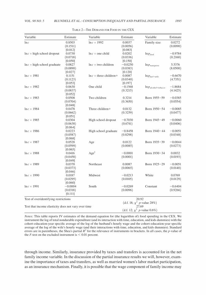
where f is the log of real food expenditure (which is available in both surveys), W and p contain a set of, respectively, demographic variables and relative prices (also available in both datasets), c is the log of nondurable expenditure (available only in the CEX), and e captures unobserved het-erogeneity in the demand for food and measurement error in food expenditure. We allow the elas-ticity b 1 · 2 (from now on, the budget elasticity) to vary with time and with observable household characteristics (D). The estimation results for our specification of (1) are reported in Table 2. To account for measurement error of total expenditure, we instrument the latter with the average (by cohort, year, and education) of the hourly wage of the husband and the average (also by cohort, year, and education) of the hourly wage of the wife. The budget elasticity is 0.85. The price elasticity is 20.98. We test the overidentifying restrictions and fail to reject the null hypothesis ( p-value of 28 percent). We also report statistics for judging the power of excluded instruments. They are all acceptable. Finally, we test whether the budget elasticity has remained constant over this period, and reject the hypothesis ( p-value 1 percent). Generally the demographics have the expected sign. Armed with these estimates, we invert the demand function and derive a series of imputed nondurable consumption for all households in the PSID.
But how good is the imputation? In an annex to this paper, we review the conditions that make the imputation procedure reliable.11 Given that our preferred measure of inequality is the variance of the logs, we require that the evolution of the variance of the imputed log consump-tion series in the PSID mirrors that of the variance of the log consumption series in the CEX. A reliable imputation procedure requires that the variance of log consumption in the PSID differs from the CEX analog only by an additive factor (the variance of the error term of the demand equation scaled by the square of the budget elasticity); if this factor is constant over time, the trends in the two variances should be similar. Figure 3 shows that the variances line up extremely well. As in Figure 1, we eliminate the level effect by rescaling the PSID consumption axis (on the left) to match that for CEX consumption (on the right). Trends in the variance of consump-tion are remarkably similar in the two datasets. In fact, the reader can check that the variance of imputed PSID consumption is just an upward-translated version (by about 0.06 units) of the variance of CEX consumption. Both series suggest that between 1980 and 1986 consumption inequality grows quite substantially. Afterward, both graphs are flat. In the annex, we show that this result is robust to variation in equivalence scales; we also show that our imputation proce-dure is capable of replicating quite well the trends in mean spending as long as account is made for differences in the mean of the input variable (food spending) in the two datasets.
II. Consumption Inequality, Insurance, and the Durability of Income Shocks
To motivate the procedure for identifying the degree of transmission of income shocks to con-sumption, we propose a framework that focuses on the persistence of income shocks. We assume that the sole relevant source of idiosyncratic uncertainty faced by the consumer is net family income (defined as the sum of labor income and transfers, such as welfare payments, minus taxes paid). We also make the assumption of separability in preferences between consumption and leisure. This implies that all insurance provided through, say, an added worker effect will pass
11 The annex is available on the AER Web site, (http://www.aeaweb.org/articles.php?doi=10.1257/aer.98.5.1887).
VOL. 98 NO. 5 1895BLuNDELL ET AL.: CONSumPTION INEquALITy AND PARTIAL INSuRANCE
through income. Similarly, insurance provided by taxes and transfers is accounted for in the net family income variable. In the discussion of the partial insurance results we will, however, exam-ine the importance of taxes and transfers, as well as married women’s labor market participation, as an insurance mechanism. Finally, it is possible that the wage component of family income may
Table 2—The Demand for Food in the CEX
Variable Estimate Variable Estimate Variable Estimate
ln c 0.8503 ln c 3 1992 0.0037 Family size 0.0272 10.15112 10.00562 10.00902 [0.012] [0.083]ln c 3 high school dropout 0.0730 ln c 3 one child 0.0202 ln pfood 20.9784 10.07182 10.03362 10.21602 [0.050] [0.150]ln c 3 high school graduate 0.0827 ln c 3 two children 20.0250 ln ptransports 5.5376 10.08902 10.03832 18.05002 [0.027] [0.120]ln c 3 1981 0.1151 ln c 3 three children1 0.0087 ln pfuel1utils 20.6670 10.11232 10.03402 14.73512 [0.053] [0.197]ln c 3 1982 0.0630 One child 20.1568 ln palcohol1tobacco 21.8684 10.08372 10.32152 14.14252 [0.052]ln c 3 1983 0.0508 Two children 0.3214 Born 1955259 20.0385 10.07042 10.36502 10.05542 [0.048]ln c 3 1984 0.0478 Three children1 0.0132 Born 1950254 20.0085 10.06622 10.32592 10.04772 [0.051]ln c 3 1985 0.0304 High school dropout 20.7030 Born 1945249 20.0060 10.06382 10.67412 10.04062 [0.064]ln c 3 1986 0.0223 High school graduate 20.8458 Born 1940244 20.0051 10.05872 10.82982 10.03482 [0.068]ln c 3 1987 0.0528 Age 0.0122 Born 1935239 20.0044 10.05992 10.00852 10.02732 [0.065]ln c 3 1988 0.0416 Age2 20.0001 Born 1930234 0.0032 10.04582 10.00012 10.01932 [0.049]ln c 3 1989 0.0370 Northeast 0.0087 Born 1925229 20.0051 10.03732 10.00652 10.01402 [0.046]ln c 3 1990 0.0187 Midwest 20.0213 White 0.0769 10.02952 10.01052 10.01292 [0.060]ln c 3 1991 20.0004 South 20.0269 Constant 20.6404 10.03182 10.00962 10.92662 [0.111]
Test of overidentifying restrictions 20.92 1d.f. 18; x2 p-value 28%2Test that income elasticity does not vary over time 27.69 1d.f. 12; x2 p-value 0.6%2Notes: This table reports IV estimates of the demand equation for (the logarithm of) food spending in the CEX. We instrument the log of total nondurable expenditure (and its interaction with time, education, and kids dummies) with the cohort-education-year specific average of the log of the husband’s hourly wage and the cohort-education-year specific average of the log of the wife’s hourly wage (and their interactions with time, education, and kids dummies). Standard errors are in parentheses, the Shea’s partial R2 for the relevance of instruments in brackets. In all cases, the p-value of the F-test on the excluded instrument is , 0.01 percent.

DECEmBER 20081896 THE AmERICAN ECONOmIC REVIEW
have already been smoothed out relative to productivity by implicit agreements within the firm. If this insurance is present, it will be reflected in the variability of income.
A. The Income Process
Our aim here is to characterize changes in the persistence of shocks to income in a reasonably flexible but parsimonious way. For this we adopt a permanent-transitory model and allow the variances of the permanent and transitory factors to vary over time. In line with many previ-ous empirical studies (Thomas MaCurdy 1982; John Abowd and David Card 1989; Moffitt and Gottschalk 1995; Costas Meghir and Pistaferri 2004), we assume that the permanent component follows a random walk.12
Suppose real (log) income, log y, can be decomposed into a permanent component P and a mean-reverting transitory component v. The income process for each household i is
(2) log yi, t 5 Z9i, t wt 1 Pi, t 1 vi, t,
where t indexes time and Z is a set of income characteristics observable and known by consumers at time t. As we note below, these will include demographic, education, ethnic, and other vari-ables. We allow the effect of such characteristics to shift with calendar time and we also allow for cohort effects.
12 For example, Moffitt (1997) writes, “In the micro-level literature on earnings dynamics, Thomas MaCurdy, Abowd and Card, and Gottschalk and I all find evidence—also from the PSID—for a random walk in individual earnings in the United States” (p. 289). Recent work on income dynamics, of which Fatih Guvenen (2006) is a leading example, has focused on models that allow less overall persistence and more general heterogeneous lifetime income profiles. It would be a very useful exercise to extend the model of partial insurance we develop here to such alterna-tive income processes. The key result of the changing persistence of income shocks and their impact on consumption inequality, however, seems unlikely to change.
0.11
0.13
0.15
0.17
0.19
0.21
0.23
CE
X
0.18
0.2
0.22
0.24
0.26
0.28
0.3
PS
ID
1980 1982 1984 1986 1988 1990 1992Year
Var. of log(C) PSID Var. of log(C) CEX
Figure 3. CEX and New PSID Compared
VOL. 98 NO. 5 1897BLuNDELL ET AL.: CONSumPTION INEquALITy AND PARTIAL INSuRANCE
We assume that the permanent component Pi, t follows a martingale process of the form
(3) Pi, t 5 Pi, t21 1 zi, t,
where zi, t is serially uncorrelated, and the transitory component vi, t follows an MA1q 2 process, where the order q is to be established empirically:
q
vi, t 5 a uj ei, t2j j50
with u0 ; 1. It follows that (unexplained) income growth is
(4) Dyi, t 5 zi, t 1 Dvi, t,
where yi, t 5 log yi, t 2 Z9i, t wt denotes the log of real income net of predictable individual components.
B. The Transmission of Income Shocks to Consumption
We present a framework that allows us to study the degree of transmission of income shocks to consumption. We write (unexplained) change in log consumption as
(5) Dci, t 5 fi, t zi, t 1 ci, t ei, t 1 ji, t,
where ci, t is the log of real consumption net of its predictable components. We allow permanent income shocks zi, t to have an impact on consumption with a loading factor of fi, t, which may potentially vary across individuals and time; the impact of transitory income shocks ei, t is mea-sured by the loading factor ci, t . The random term ji, t represents innovations in consumption that are independent of those in income. This may capture measurement error in consumption, preference shocks, innovation to higher moments of the income process, etc. We call fi, t and ci, t partial insurance parameters.
Equation (5) nests the two extreme cases of full insurance of income shocks (fi, t 5 ci, t 5 0) as contemplated by the complete markets hypothesis, and no insurance (fi, t 5 ci, t 5 1) as in autarky, as well as intermediate cases in which 0 , fi, t , 1 and 0 , ci, t , 1. The closer the coefficient to zero, the higher is the degree of insurance.
Self-Insurance.—The most prominent intermediate case is the PIH with self-insurance through precautionary savings. Appendix B considers a version of the PIH with CRRA prefer-ences, and shows that in this case approximation of the Euler equation for consumption gives fi, t . pi, t and ci, t . gt, Lpi, t, where pi, t is the share of future labor income in current human and financial wealth and gt, L is an age-increasing annuitization factor.13 The random term ji, t can be
13 See Appendix B. As far as we know, this is the first derivation of such an expression for the marginal propensity to consume with respect to permanent shocks in a model with CRRA preferences and transitory and permanent shocks. See Christopher Carroll (2001) for numerical simulations. Results from a simulation of a stochastic economy presented in Blundell, Hamish Low, and Preston (2004) show that the approximation (B5) can be used to accurately detect changes in the time series pattern of permanent and transitory variances to income shocks. These results are available upon request (by e-mail to: [email protected]).

DECEmBER 20081898 THE AmERICAN ECONOmIC REVIEW
interpreted as the innovation to higher moments of the income process.14 Meghir and Pistaferri (2004) find evidence of this using PSID data.
The interpretation of the impact of income shocks on consumption growth in the PIH model with CRRA preferences is straightforward. For individuals who are a long time from the end of their life with the value of current financial assets small relative to remaining future labor income, pi, t . 1, and permanent shocks pass through more or less completely into consumption, whereas transitory shocks are (almost) completely insured against through saving. Precautionary saving can provide effective self-insurance against permanent shocks only if the stock of assets built up is large relative to future labor income, which is to say pi, t is appreciably smaller than unity, in which case there will also be some smoothing of permanent shocks through self insur-ance. Carroll (2001) presents simulations that show, for a buffer stock model, the steady-state value of pi, t is between 0.85 and 0.95. Blundell, Low, and Preston (2007) simulate the model described in Appendix B using our estimates of the income process and find a value of pi, t of 0.8 or a little lower for individuals 20 years of age before retirement, which corresponds to the aver-age age in our sample, finding that fi, t , pi, t and/or ci, t , gt, Lpi, t represents evidence of partial insurance over and above self-insurance through savings.
Excess Smoothness and “Excess” Insurance.—A recent macroeconomic literature has explored a number of theoretical alternatives to the insurance configurations described above. These alternative models fall under two broad rubrics: those that assume public information but limited enforcement of contracts, and those that assume full commitment but private informa-tion. These models prove that the self-insurance case is Pareto-inefficient even conditioning on limited enforcement and private information issues. In both types of models, agents typically achieve more insurance than under a model with a single noncontingent bond, but less than under a complete markets environment. More importantly for our purposes, these models show that the relationship between income shocks and consumption depends on the degree of persistence of income shocks. Fernando Alvarez and Urban Jermann (2000), for example, explore the nature of income insurance schemes in economies where agents cannot be prevented from withdraw-ing participation if the loss from the accumulated future income gains they are asked to forgo becomes greater than the gains from continuing participation. Such schemes, if feasible, allow individuals to keep some of the positive shocks to their income and therefore offer only partial income insurance. If income shocks are persistent enough and agents are infinitely lived, then participation constraints become so severe that no insurance scheme is feasible. With finite lived agents, the future benefits from a positive permanent shock exceed those from a comparable transitory shock. This suggests that the degree of insurance should be allowed to differ between transitory and permanent shocks and should also be allowed to change over time and across dif-ferent groups.
Another reason for partial insurance is moral hazard. This is the direction taken in Attanasio and Pavoni (2006). Here the economic environment is characterized by moral hazard and hidden asset accumulation, e.g., individuals have hidden access to a simple credit market. The authors show that, depending on the cost of shirking and the persistence of the income shock, some par-tial insurance is possible and a linear insurance rule can be obtained as an exact (closed form) solution in a dynamic Mirrlees model with CRRA utility. This provides a structural interpreta-
14 This characterization follows Ricardo Caballero (1990), who presents a model with stochastic higher moments of the income distribution. He shows that there are two types of innovation affecting consumption growth: innovation to the mean (the term pi, tzi, t 1 pi, tgt, Lei, t ), and “a term that takes into account revisions in variance forecast” (ji, t ). Note that this term is not capturing precautionary savings per se, but the innovation to the consumption component that gen-erates it (i.e., consumption growth due to precautionary savings will change to accommodate changes in the forecast of the amount of uncertainty one expects in the future).

VOL. 98 NO. 5 1899BLuNDELL ET AL.: CONSumPTION INEquALITy AND PARTIAL INSuRANCE
tion of the parameters in our estimated model. In particular, the response of consumption to per-manent income shocks (what we call the partial insurance coefficient in our framework) could be interpreted as a measure of the severity of informational problems. Their empirical analysis finds evidence for “excess smoothness” of consumption with respect to permanent shocks.
Advance Information.—In the analysis presented thus far we have assumed that in the innova-tion process for income (4), the random variables zi, t and ei, t represent the arrival of new infor-mation to agent i in period t. If parts of these random terms were known in advance to the agent, then the intertemporal consumption model would argue that they should already be incorporated into current plans and would not directly effect consumption growth (5) (see Flavio Cunha, James Heckman, and Salvador Navarro 2005). Suppose, for example, that only a proportion k of the permanent shock was unknown to the consumer. Then the consumption growth relationship (5) would become
(6) Dci, t . f̃i, t k zi, t 1 ci, tei, t 1 ji, t ,
where f̃i, t is the “true” insurance parameter. In this case, f̃i, t would be underestimated by the information factor k (i.e., we would call insurance what is, in fact and in part, advance information).15
The econometrician will treat zi, t as the permanent shock, whereas the individual may have already adapted to this change. Consequently, although transmission of income inequality to consumption inequality is correctly identified, the estimated fi, t has to be interpreted as reflect-ing a combination of insurance and information. In the absence of outside information (such as, say, subjective expectations), these two components cannot be separately identified. However, in our empirical analysis of the autocovariance structure of income and consumption, we provide some evidence that advance information is not a serious problem during our sample period. In particular, we show that current consumption growth is not significantly correlated with future “shocks” to income.
C. Evolution of Income and Consumption Variances
We assume that zi, t , vi, t, and ji, t are mutually uncorrelated processes. As in Hall and Mishkin (1982) and others, one can impose covariance restrictions on the bivariate process (4) and (5) to identify the parameters of interest. In particular, equation (4) can be used to derive the following covariance restrictions in panel data:
var 1zt 2 1 var 1Dvt 2 for s 5 0(7) cov 1Dyt, Dyt1s 2 5 • , cov 1Dvt, Dvt1s 2 for s Z 0
where var 1 · 2 and cov 1 · , · 2 denote cross-sectional variances and covariances, respectively (the index i is consequently omitted). These moments can be computed for the whole sample or for individuals belonging to a homogeneous group (i.e., born in the same year, with the same level of schooling, etc.). The covariance term cov 1Dvt , Dvt1s 2 depends on the serial correlation prop-erties of v. If v is an MA1q 2 serially correlated process, then cov 1Dvt , Dvt1s 2 is zero whenever
15 Another source of downward bias would result if the permanent component were less persistent than a martingale. As the p parameter reflects the annuity value of the shock, if the z shock was less persistent than implied by a unit root, this would also lead to a value of f less than unity.

DECEmBER 20081900 THE AmERICAN ECONOmIC REVIEW
Z s Z . q 1 1. Note also that if v is serially uncorrelated (vi, t 5 ei, t ), then var 1Dvt 2 5 var 1et 2 1 var 1et212 . Identification of the serial correlation coefficients does not hinge on the order of the process q. Allowing for an MA1q 2 process, for example, adds q 2 1 extra parameters (the q 2 1 MA coefficients) but also q 2 1 extra moments, so that identification is unaffected. Equation (7) shows that income inequality (obtained setting s 5 0) may increase either because of increases in the variance of permanent shocks, or because of an increase in the variance of income growth due to transitory shocks.
The panel data restrictions on consumption growth from (5) are as follows: 16
(8) cov 1Dct , Dct1s 2 5 ft2 var 1zt 2 1 ct
2 var 1et 2 1 var 1jt 2
for s 5 0, and zero otherwise (due to the consumption martingale assumption). This equation shows that consumption growth inequality (s 5 0) can rise for two reasons: a decline in the degree of insurance with respect to income shocks (for given variances), or an increase in the variances of income shocks (for given insurance). In other words (assuming ji, t is stationary), one can write the following decomposition for the time change in the variance of consumption growth:
Dvar 1Dct 2 5 var 1zt 2Dft2 1 f2
t21 Dvar 1zt 2 1 var 1et 2Dct2 1 c2
t21Dvar 1et 2 .
Our analysis below allows separation of the different forces at play visible in this equation. Finally, the covariance between income growth and consumption growth at various lags is
ftvar 1zt 2 1 ctvar 1et 2(9) cov 1Dct , Dyt1s 2 5 • , ct cov 1et, Dvt1s 2
for s 5 0 and s . 0, respectively. If v is an MA1q 2 serially correlated process, then cov 1Dct , Dyt1s 2 is zero whenever Z s Z . q 1 1. Thus, if v is serially uncorrelated (vi, t 5 ei, t ), then cov 1Dct , Dyt1s 2 5 2ctvar 1et 2 for s 5 1, and 0 otherwise.
Note, finally, that it is likely that measurement error will contaminate the observed income and consumption data. Assume that both consumption and income are measured with multiplica-tive independent errors, e.g.,
(10) y*i, t 5 yi, t 1 uy
i, t,
(11) c*i, t 5 ci, t 1 uc
i, t,
where x* denotes a measured variable, x its true, unobservable value, and ux the measurement error.
In Appendix C we discuss identification details of the model more in detail, and also show that the partial insurance parameter ft remains identified under measurement error, while only a lower bound for ct is identifiable. A corollary of this is that the variance of measurement error in consumption can be identified (the theory suggests that consumption should be a martingale with drift, so any serial correlation in consumption growth can only be attributed to noise), but the variance of the measurement error in income can still not be identified separately from the
16 The errors of approximation on these expressions are of the order of the expected values of the cubes of Zzt Z and Zet Z.

VOL. 98 NO. 5 1901BLuNDELL ET AL.: CONSumPTION INEquALITy AND PARTIAL INSuRANCE
variance of the transitory shock.17 The goal of the empirical analysis is to estimate features of the distribution of income shocks (variances of permanent and transitory shocks and the extent of serial correlation in the latter) and consumption growth (particularly the partial insurance parameters) using joint panel data on income and consumption growth on which the theoretical restrictions (7)–(9) have been imposed.
In the context of identifying sources of variation in household income and consumption, the availability of panel data presents several advantages over a repeated cross-sections analysis. With repeated cross sections the variances and covariances of differences in income and con-sumption cannot be observed, although it is possible to make assumptions under which variances of shocks can be identified from differences in variances and covariances of their levels (assum-ing one knows the degree of insurance with respect to income shocks). For example, under the assumption that shocks are cross-sectionally orthogonal to past consumption and income, that transitory shocks are serially uncorrelated, and that ft 5 1 and ct 5 0, Blundell and Preston (1998) use repeated cross-section moments to separate the growth in the variance of transitory shocks to log income from the variance of permanent shocks (see also Deaton and Paxson 1994). The assumed orthogonality assumption will be violated if aggregate consumption (or income) is not part of the consumer’s information set (see Deaton and Paxson 1994). In panel data, identi-fication does not require making such assumption and can allow for serial correlation in transi-tory shocks as well as measurement error in consumption and income data (see below). More crucially, with panel data one can estimate a richer model with the insurance parameter ft and ct left free and thus test the validity of alternative explanations regarding the evolution of consump-tion inequality over time. In turn, knowledge of the extent of insurance is informative about the welfare effects of shifts in the income distribution. In our application we allow partial insurance parameters to differ by cohorts and interpret differences over time as year rather than age effects, although we appreciate that the choice is an arbitrary one made only for descriptive clarity.
Note, finally, that with panel data the identification of the variances of shocks to income requires only panel data on income, not consumption. In the simple case of serially uncorrelated transitory shock, for example,18
(12) var 1zt 2 5 cov 1Dyt, Dyt21 1 Dyt 1 Dyt112 ,
(13) var 1et 2 5 2cov 1Dyt, Dyt112 .
Using panel data on both consumption and income improves efficiency of these estimates because it provides extra moments for identification.
III. The Evidence
The parameters of interest in this study are the insurance parameters, f and c, and the evo-lution of inequality in the permanent and transitory components to income. They are derived from the variance-covariance structure of changes in consumption and income. We consequently begin with the empirical characterization of these autocovariances. We then evaluate the rela-tive size and trends in the variance of permanent and transitory shocks to income and estimate
17 Thus, the variance of measurement error in consumption is identified by 2cov 1Dct , Dct112 .18 See Meghir and Pistaferri (2004) for a generalization to serially correlated transitory shocks and measurement
error in income. In their paper, they show that with an MA(q) process for the transitory shock, one needs T 5 4 1 q years of data to identify the variances of interest. Given that we have access to a panel of 15 years, this condition is amply satisfied.

DECEmBER 20081902 THE AmERICAN ECONOmIC REVIEW
the degree of insurance to these shocks for the entire sample and for different subgroups of the population.
A. The Autocovariance of Consumption and Income
The impact of the deterministic effects Zit on log income and (imputed) log consumption is removed by separate regressions of these variables on year and year-of-birth dummies, and on a set of observable family characteristics (dummies for education, race, family size, number of children, region, employment status, residence in a large city, outside dependent, and presence of income recipients other than husband and wife). We allow for the effect of most of these characteristics to vary with calendar time. We then work with the residuals of these regressions, labelled ci, t and yi, t .19
To pave the way to the formal analysis of partial insurance, Table 3 reports unrestricted minimum distance estimates of several moments of the income process for the whole sample: the variance of unexplained income growth, var 1Dyt 2 , the first-order autocovariances, 1cov 1Dyt11, Dyt 2 2 , and the second-order autocovariances, 1cov 1Dyt12, Dyt 2 2 . Estimates are reported for each year. Table 4 repeats the exercise for our new panel data measure of con-sumption. Finally, Table 5 reports minimum distance estimates of contemporaneous and lagged consumption-income covariances. As noted above, some of the moments are miss-ing because consumption data were not col-lected in the PSID in the 1987–1988 period.
Looking at Table 3, one can notice the strong increase in the variance of income growth, rising by more than 30 percent by 1985. Also notice the blip in the final year (in 1992 the PSID converted the question-naire to electronic form and imputations of income were done by machine). The absolute value of the first-order autocovariance also increases until the mid-1980s and then is stable or even declines. Second- and higher-order autocovariances (which, from equa-tion (7), are informative about the presence of serial correlation in the transitory income component) are small and only in few cases statistically significant. At least at face value, this evidence seems to tally quite well with a canonical MA(1) process in growth, as implied by an income process given by the sum of a martingale permanent component
19 To the extent that these regressions remove changes that are unexpected by the individuals, we might expect this to change the relative degree of persistence in the remaining shocks, but not the insurance parameters. For example, by removing the effect of education-time on income and consumption, we are also removing the increase in inequality due to, say, changing education premiums (Attanasio and Davis 1996). If we omit the education variables from our first stage, we find that it makes only a small difference to the estimated insurance parameters (for example, the estimate of f in Table 6 below is 0.71 instead of 0.64). The same qualitative comment applies to the other variables whose effect is removed in the first stage.
Table 3—The Autocovariance Matrix of Income Growth
Year var 1Dyt 2 cov 1Dyt11, Dyt 2 cov 1Dyt12, Dyt 21980 0.0832 20.0196 20.0018 (0.0089) (0.0035) (0.0032)1981 0.0717 20.0220 20.0074 (0.0075) (0.0034) (0.0037)1982 0.0718 20.0226 20.0081 (0.0051) (0.0035) (0.0026)1983 0.0783 20.0209 20.0094 (0.0066) (0.0034) (0.0042)1984 0.0805 20.0288 20.0034 (0.0055) (0.0036) (0.0032)1985 0.1090 20.0379 20.0019 (0.0180) (0.0074) (0.0038)1986 0.1023 20.0354 20.0115 (0.0077) (0.0054) (0.0038)1987 0.1116 20.0375 0.0016 (0.0097) (0.0051) (0.0046)1988 0.0925 20.0313 20.0021 (0.0080) (0.0042) (0.0032)1989 0.0883 20.0280 20.0035 (0.0067) (0.0059) (0.0034)1990 0.0924 20.0296 20.0067 (0.0095) (0.0049) (0.0050)1991 0.0818 20.0299 NA (0.0059) (0.0040) 1992 0.1177 NA NA (0.0079)

VOL. 98 NO. 5 1903BLuNDELL ET AL.: CONSumPTION INEquALITy AND PARTIAL INSuRANCE
and a serially uncorrelated transitory compo-nent. Since evidence on second-order autoco-variances is mixed, however, in estimation we allow for MA(1) serial correlation in the transi-tory component 1vi, t 5 ei, t 1 uei, t212 .20
While income moments are informative about shifts in the income distribution (and on the temporary or persistent nature of such shifts), they cannot be used to make conclusive inference about shifts in the consumption dis-tribution. For this purpose, one needs to com-plement the analysis of income moments with that of consumption moments and of the joint income-consumption moments. This is done in Tables 4 and 5. Table 4 shows that the variance of imputed consumption growth also increases quite strongly in the early 1980s, peaks in 1985, and then it is essentially flat afterward. Note the high value of the level of the vari-ance, which is clearly the result of our imputa-tion procedure. The variance of consumption growth captures in fact the genuine association with shocks to income, but also the contribu-tion of slope heterogeneity and measurement error.21 The absolute value of the first-order
autocovariance of consumption growth should be a good estimate of the variance of the imputa-tion error. This is in fact quite high. Second-order and higher consumption growth autocovari-ances are mostly statistically insignificant and economically small.
Table 5 examines the association, at various lags, of unexplained income and consumption growth. The contemporaneous covariance should be informative about the effect of income shocks on consumption growth if measurement errors in consumption are orthogonal to mea-surement errors in income. This covariance increases in the early 1980s and then is flat or even declining afterward.
From (9), the covariance between current consumption growth and one-period-ahead income growth cov 1Dct, Dyt112 should reflect the extent of insurance with respect to transitory shocks (i.e., cov 1Dct, Dyt112 5 0 if there is full insurance of transitory shocks). We note that in the pure self-insurance case with infinite horizon and MA(1) transitory component, the impact of transi-tory shocks on consumption growth is given by the annuity value r 11 1 r 2 u 2/ 11 1 r 22. With a small interest rate, this will be indistinguishable from zero, at least statistically. In fact, this cova-riance is hardly statistically significant and economically close to zero. At the foot of Table 5 we present the p-values for the joint significance tests of the autocovariances E 1Dct, Dyt1j 2 1 j $ 12 . These p-values also detect advance information. If future income shocks were known to the consumer in earlier periods, then consumption should adjust before the observed shock occurs. This should show up in significant autocovariances between changes in consumption and future
20 We also estimated the autocovariances of income growth at lags greater than two and find that none of them is statistically significant. These results are available from the authors upon request.
21 To a first approximation, the variance of consumption growth that is not contaminated by error can be obtained by subtracting twice the (absolute value of) first-order autocovariance cov 1Dct11, Dct 2 from the variance var 1Dct 2 .
Table 4—The Autocovariance Matrix of Consumption Growth
Year var 1Dct 2 cov 1Dct11, Dct 2 cov 1Dct12, Dct 21980 0.1275 20.0526 0.0022 (0.0097) (0.0076) (0.0056)1981 0.1197 20.0573 0.0025 (0.0116) (0.0084) (0.0043)1982 0.1322 20.0641 0.0006 (0.0110) (0.0087) (0.0060)1983 0.1532 20.0691 20.0056 (0.0159) (0.0100) (0.0067)1984 0.1869 20.1003 20.0131 (0.0173) (0.0163) (0.0089)1985 0.2019 20.0872 NA (0.0244) (0.0194) 1986 0.1628 NA NA (0.0184) 1987 NA NA NA 1988 NA NA NA 1989 NA NA NA 1990 0.1751 20.0602 20.0057 (0.0221) (0.0062) (0.0067)1991 0.1646 20.0696 NA (0.0142) (0.0100) 1992 0.1467 NA NA (0.0130)

DECEmBER 20081904 THE AmERICAN ECONOmIC REVIEW
incomes. We find no statistical evidence, how-ever, that this is the case.
The covariance between current con-sumption growth and past income growth cov 1Dct11, Dyt 2 plays no role in the PIH model with perfect capital markets, but may be important in alternative models where liquidity constraints are present (a standard excess sen-sitivity argument; see Marjorie Flavin 1981). The estimates of this covariance in Table 5 are also close to zero.
To sum up, the evidence suggests that a simple permanent-transitory framework for income shocks with time-varying second-order moments in these shocks provides a good representation of the income process for fami-lies in the PSID over this period. Overall we find only weak evidence that transitory shocks affect consumption growth. In the sensitivity results reported below, however, we find that there is evidence of significant responsiveness to transitory shocks for low-wealth families and for the low-income poverty sample of the PSID.
B. Insurance
Our focus here will be on the variances of the permanent and the transitory shock, sz
2 and se
2, on the partial insurance coefficients for the permanent shock (f) and for the transitory shock (c), and the way these parameters vary over time, as well as among different groups in the popu-lation. Our estimates are based on a generalization of moments (7)–(9). In particular, to account for our imputation procedure, we allow consumption to be measured with error, and we allow the variance of the measurement error in consumption to vary with time. This is to capture the fact that the imputation error is scaled by a time-varying budget elasticity which induces non-stationarity. We also consider an MA(1) process for the transitory error component of income 1vi, a, t 5 ei, t 1 uei, t212 , and estimate the MA(1) parameter u. Finally, we allow for i.i.d. unobserved heterogeneity in the individual consumption gradient, and estimate its variance (sj
2 ).We present the results of three specifications: one for the whole sample (the “baseline” speci-
fication), one where the parameters are estimated separately by education (college versus no college), and one where parameters are estimated separately by cohort (born 1930s versus born 1940s).22 We also allow for some time nonstationarity. In particular, in all specifications we let the variances of the permanent and the transitory shock, sz
2 and se2 , respectively, vary with calen-
dar time. As for the partial insurance coefficients for the permanent shock (f) and for the transi-tory shock (c), we assume that they take on two different values, before and after 1985. This is consistent with the evidence in Figure 1, which divides the sample period into a period of rapid
22 Results for the younger cohort (born in the 1950s) and the older cohort (born in the 1920s) are less reliable because these cohorts are not observed for the whole sample period. We thus omit them.
Table 5—The Consumption-Income Growth Covariance Matrix
Year cov 1Dyt, Dct 2 cov 1Dyt11, Dct 2 cov 1Dyt, Dct1121980 0.0040 0.0013 0.0053 (0.0041) (0.0039) (0.0037)1981 0.0116 20.0056 20.0043 (0.0036) (0.0032) (0.0036)1982 0.0165 20.0064 20.0006 (0.0036) (0.0031) (0.0039)1983 0.0215 20.0085 20.0075 (0.0045) (0.0049) (0.0043)1984 0.0230 20.0030 20.0119 (0.0052) (0.0043) (0.0050)1985 0.0197 20.0035 20.0035 (0.0068) (0.0047) (0.0065)1986 0.0179 20.0015 NA (0.0048) (0.0052) 1987 NA NA NA 1988 NA NA NA 1989 NA NA 0.0030 (0.0040)1990 0.0077 0.0045 20.0016 (0.0045) (0.0065) (0.0042)1991 0.0112 0.0011 20.0071 (0.0044) (0.0049) (0.0042)1992 0.0082 NA NA (0.0048) Test cov 1Dyt11, Dct 2 5 0 for all t p-value 25%Test cov 1Dyt12, Dct 2 5 0 for all t p-value 27%Test cov 1Dyt13, Dct 2 5 0 for all t p-value 74%Test cov 1Dyt14, Dct 2 5 0 for all t p-value 68%

VOL. 98 NO. 5 1905BLuNDELL ET AL.: CONSumPTION INEquALITy AND PARTIAL INSuRANCE
growth in the variance (up until 1985), and one of relative stability afterward. We test the null that the extent of insurance does not change over time, and with almost no exceptions we fail to reject the null. In the discussion of the results that follows we comment on the time variability of the insurance parameters where appropriate and present the results of the test in the tables.
The parameters are estimated by diagonally weighted minimum distance (DWMD). This esti-mation method is a simple generalization of equally weighted minimum distance (EWMD). Unlike EWMD, it allows for heteroskedasticity. Moreover, it avoids the pitfalls of optimal mini-mum distance (OMD) remarked by Altonji and Lewis Segal (1996), which are primarily related to the terms outside the main diagonal of the optimal weighting matrix. Technical details are in Appendix D.23
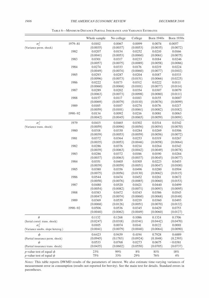
The first column of Table 6 shows the results for the whole sample. We defer the discussion of the estimated variances of the permanent shock and the estimated variances of the transitory shock to the next paragraph. The MA parameter for the transitory shock is small. The estimates of the variance of the imputation error (not reported) are always precisely measured and suggest that the imputation error absorbs a large amount of the cross-sectional variability in consump-tion (the estimates vary between 0.05 and 0.10). The variance of unobserved heterogeneity in the consumption gradient is small but significant. In the whole sample the estimate of f, the partial insurance coefficient for the permanent shock, provides evidence in favor of some partial insurance.24 In particular, a 10 percent permanent income shock induces a 6.4 percent permanent change in consumption.25 The evidence on c accords with a simple PIH model with a long hori-zon.26 If we allow the partial insurance parameters to vary across time, then we find a slightly lower estimate of f—indicating more insurance—in the later part of the 1980s. This would be in line with the idea developed in Krueger and Perri (2006) that a higher variance provides additional incentives to insure. However, the differences in the partial insurance parameters over this time period are small and are not statistically significant. Hence we decided to restrict the coefficient to be constant over the whole period. The p-values for the test of constant insurance parameters over the two subperiods are given in the last two rows of the table.27
There is much discussion in the literature on the reasons for the increase in income inequality over the 1980s. In particular, there is much debate on whether the rise can be labeled permanent or transitory. In Figure 4 we plot the minimum distance estimate of the variance of the permanent shock, var 1zt 2 , against time. There are two sets of estimates. One uses the full set of consump-tion and income moments for the baseline specification in Table 6, and another utilizes only the income data. There is a close accordance between the two series which provides a check on the validity of our specification. The figure points to strong growth in permanent income shocks during the early 1980s. The variance of permanent shocks levels off thereafter. It is also worth
23 If we use EWMD, we obtain extremely downward biased estimates of var 1zt 2 and extremely upward biased esti-mates of var 1et 2 (compared to those we obtain using income data only, as in (12) and (13)). With DWMD the two sets of estimates are similar because we are effectively putting more “identification weight” for the income shock variances on the income moments and less on the consumption moments (which display more sampling variability due to the imputation procedure).
24 As shown in the Appendix, if income is measured with error, the estimate of sj2 1c 2 is upward (downward) biased.
However, the bias is likely negliglible (see the Appendix for an example).25 This “excess smoothness” result has been replicated in recent papers by Attanasio and Pavoni (2006), Primiceri
and Van Rens (2007), and Heathcote, Storesletten, and Violante (2007).26 If we assume that food in the PSID reported in survey year t refers to that year rather than to the previous calendar
year, we obtain similar results. The estimate of f is slightly higher, but the qualitative pattern of results (and sensitivity checks) is unchanged.
27 We note that the overall results are maintained by extending the data forward until 1996. These results are avail-able from the authors upon request.
DECEmBER 20081906 THE AmERICAN ECONOmIC REVIEW
Table 6—Minimum-Distance Partial Insurance and Variance Estimates
Whole sample No college College Born 1940s Born 1930s
sz2 1979–81 0.0102 0.0067 0.0099 0.0074 0.0057
1Variance perm. shock2 10.00352 10.00372 10.00532 10.00352 10.00722 1982 0.0207 0.0154 0.0252 0.0210 0.0166 10.00412 10.00532 10.00602 10.00612 10.00752 1983 0.0301 0.0317 0.0233 0.0184 0.0246 10.00572 10.00752 10.00892 10.00582 10.00862 1984 0.0274 0.0333 0.0176 0.0219 0.0224 10.00492 10.00742 10.00602 10.00772 10.01022 1985 0.0293 0.0287 0.0204 0.0187 0.0333 10.00962 10.00732 10.01512 10.00662 10.02252 1986 0.0222 0.0173 0.0312 0.0222 0.0111 10.00602 10.00682 10.01012 10.00772 10.01142 1987 0.0289 0.0202 0.0354 0.0307 0.0079 10.00632 10.00732 10.00982 10.00802 10.01112 1988 0.0157 0.0117 0.0183 0.0155 0.0007 10.00692 10.00792 10.01102 10.00762 10.00992 1989 0.0185 0.0107 0.0274 0.0176 0.0217 10.00592 10.01012 10.00612 10.00822 10.01822 1990–92 0.0134 0.0092 0.0216 0.0081 0.0063 10.00422 10.00452 10.00652 10.00592 10.00912 se
2 1979 0.0415 0.0465 0.0302 0.0314 0.03421Variance trans. shock 2 10.00592 10.00962 10.00562 10.00542 10.00702 1980 0.0318 0.0330 0.0284 0.0269 0.0306 10.00392 10.00532 10.00592 10.00562 10.00722 1981 0.0372 0.0364 0.0253 0.0319 0.0267 10.00352 10.00532 10.00462 10.00582 10.00642 1982 0.0286 0.0376 0.0214 0.0264 0.0342 10.00392 10.00632 10.00422 10.00492 10.00782 1983 0.0286 0.0372 0.0186 0.0190 0.0284 10.00372 10.00632 10.00372 10.00452 10.00772 1984 0.0351 0.0405 0.0305 0.0223 0.0453 10.00392 10.00592 10.00512 10.00472 10.01002 1985 0.0380 0.0356 0.0496 0.0280 0.0504 10.00752 10.00562 10.01302 10.00622 10.01152 1986 0.0544 0.0474 0.0452 0.0261 0.0672 10.00582 10.00762 10.00852 10.00602 10.01532 1987 0.0480 0.0520 0.0421 0.0440 0.0499 10.00542 10.00822 10.00712 10.00932 10.00952 1988 0.0383 0.0472 0.0343 0.0386 0.0543 10.00472 10.00742 10.00602 10.00682 10.01482 1989 0.0369 0.0539 0.0219 0.0360 0.0493 10.00682 10.01262 10.00512 10.00702 10.01322 1990–92 0.0506 0.0536 0.0345 0.0429 0.0753 10.00402 10.00622 10.00492 10.00602 10.01272 u 0.1132 0.1268 0.1086 0.1324 0.17061Serial correl. trans. shock 2 10.02472 10.03182 10.03412 10.04422 10.04702 sj
2 0.0105 0.0074 0.0141 0.0122 0.00011Variance unobs. slope heterog.2 10.00412 10.00792 10.00402 10.00642 10.00902 f 0.6423 0.9439 0.4194 0.7928 0.68891Partial insurance perm. shock2 10.09452 10.17832 10.09242 10.18482 10.23932 c 0.0533 0.0768 0.0273 0.0675 20.03811Partial insurance trans. shock 2 10.04352 10.06022 10.05502 10.07052 10.07372p-value test of equal f 23% 99% 8% 81% 18%p-value test of equal c 75% 33% 29% 76% 4%
Notes: This table reports DWMD results of the parameters of interest. We also estimate time-varying variances of measurement error in consumption (results not reported for brevity). See the main text for details. Standard errors in parentheses.

VOL. 98 NO. 5 1907BLuNDELL ET AL.: CONSumPTION INEquALITy AND PARTIAL INSuRANCE
noting that from trough to peak the variance of the permanent shock more than doubles.28 This evidence on permanent shocks is similar to that reported by Moffitt and Gottschalk (1995) using PSID data on male earnings. As we will document below, however, the precise evolution of inequality in transitory shocks depends on the source of income under study. Male labor earnings data will be shown to display a higher transitory variance in the earlier part of this time period.
Table 6 also reports the results of the model for two education groups (with and without col-lege education), and for two representative birth cohorts (born in the 1940s and born in the 1930s).29 The partial insurance parameter estimates point to interesting differences in insurance by type of household. In particular, there appears to be less insurance in response to permanent shocks among the group with no college education (indeed, we would not statistically reject the null hypothesis that there is no insurance in this group). In contrast, the evidence on c accords with a simple PIH model and we cannot reject the null that there is full smoothing with respect to transitory shocks (c 5 0) for both education groups, though for the less well educated the point estimate is higher.
When the sample is stratified by year of birth, we find qualitatively similar results: there is evidence for full insurance with respect to transitory shocks and differences in the extent of insurance with respect to the permanent shocks.30 It is worth considering whether the presence of precautionary asset accumulation is an explanation for the pattern of results. Recall that the insur-ance coefficients may reflect differences in pi, t (the share of future labor income in the present value of lifetime wealth), which in our framework reflects how close an individual is to retirement age. Thus, pi, t is likely to be lower for older cohorts because they have both more accumulated financial wealth and lower prospective human capital wealth. Indeed, we find some evidence that
28 An even more striking accordance between the two alternative estimates is found for the estimated variances of the transitory shock, which we omit here.
29 Since we stratify the sample by exogenous characteristics and estimate different parameters for different groups, we are effectively considering the insurability of shocks within groups.
30 We find qualitatively similar results if we relax the age requirement (including those between the age of 25 and 30). The estimate of f is 0.70 (s.e. 0.10), indicating slightly less insurance to permanent shocks. This can be interpreted as reflecting a longer horizon among younger individuals. The estimate of c is 0.06 (s.e. 0.04).
Figure 4. Variance of Permanant Shocks in the 1980s
0
0.01
0.02
0.03
0.04
1980 1985 1990Year
Using cons. and income data Using only income data

DECEmBER 20081908 THE AmERICAN ECONOmIC REVIEW
permanent shocks for the older cohort are smoothed to a greater extent than for younger cohorts, although these subgroup estimates are less precise. Whether this is due to the effect played by precautionary wealth accumulation remarked above or by greater availability of insurance (such as social security, disability insurance, or even insurance provided by adult children) in the group of persons born in the 1930s is something we cannot address in the absence of additional informa-tion, such as panel data on assets and age-specific estimates of human capital wealth. Later we provide some suggestive evidence that wealth accumulation is a potentially important explanation for the degree of insurance with respect to permanent income shocks.31
How good is the fit of our model? In Figure 5 we plot the actual variance of income growth and its predicted value (the dashed line) from our baseline model. We repeat the exercise for the variance of consumption growth and the covariance between income and consumption growth. Our model appears to fit the model quite well in all three dimensions.
Before delving into more detail concerning the underlying mechanisms at work in our results, we ask the question: could these baseline results have been obtained using food data alone? With almost no exceptions, all the papers in the literature (including Hall and Mishkin 1982; Hayashi, Altonji, and Kotlikoff 1996) use the PSID data on food, so it is worth asking what is the value added of using our imputed measure of consumption. A possible argument in favor of this simpler approach is that food is a constant fraction of nondurable expenditure, so that the
31 In a separate experiment (not reported for brevity), we exploited variability across cohorts and allowed the insur-ance parameters f and c to depend on age. We fit a linear age trend by minimum distance: fa 5 f0 1 f1age 1 e, where e is an error. We find evidence of a decline in the value of f by age (consistent with precautionary saving), but the estimates are not very precise. We also tried a quadratic age trend, but the fit worsened. A difference statistic would favor the linear trend specification.
0.1
0.14
0.18
0.22
1980 1982 1984 1986 1988 1990 1992Year
Var(Dlog(c))
0.06
0.08
0.1
0.12
1980 1982 1984 1986 1988 1990 1992Year
Var(Dlog(y))
00.
010.
020.
03
1980 1982 1984 1986 1988 1990 1992Year
Cov(Dlog(c),Dlog(y))
Figure 5. Goodness of Fit of the Model
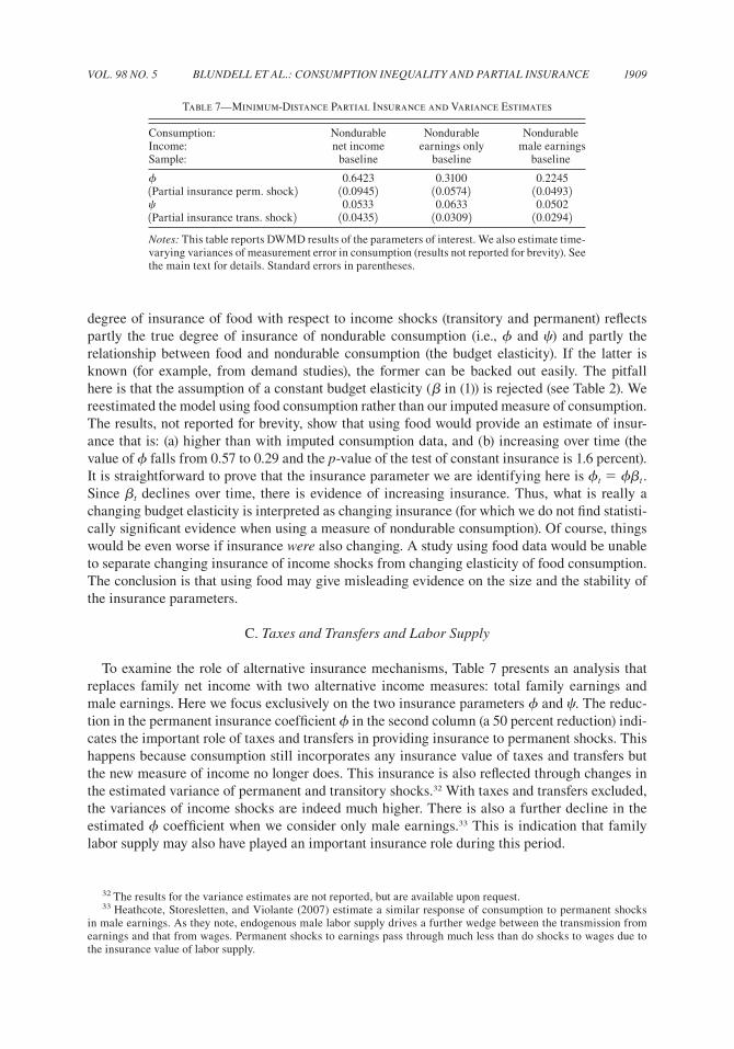
VOL. 98 NO. 5 1909BLuNDELL ET AL.: CONSumPTION INEquALITy AND PARTIAL INSuRANCE
degree of insurance of food with respect to income shocks (transitory and permanent) reflects partly the true degree of insurance of nondurable consumption (i.e., f and c) and partly the relationship between food and nondurable consumption (the budget elasticity). If the latter is known (for example, from demand studies), the former can be backed out easily. The pitfall here is that the assumption of a constant budget elasticity (b in (1)) is rejected (see Table 2). We reestimated the model using food consumption rather than our imputed measure of consumption. The results, not reported for brevity, show that using food would provide an estimate of insur-ance that is: (a) higher than with imputed consumption data, and (b) increasing over time (the value of f falls from 0.57 to 0.29 and the p-value of the test of constant insurance is 1.6 percent). It is straightforward to prove that the insurance parameter we are identifying here is ft 5 fbt . Since bt declines over time, there is evidence of increasing insurance. Thus, what is really a changing budget elasticity is interpreted as changing insurance (for which we do not find statisti-cally significant evidence when using a measure of nondurable consumption). Of course, things would be even worse if insurance were also changing. A study using food data would be unable to separate changing insurance of income shocks from changing elasticity of food consumption. The conclusion is that using food may give misleading evidence on the size and the stability of the insurance parameters.
C. Taxes and Transfers and Labor Supply
To examine the role of alternative insurance mechanisms, Table 7 presents an analysis that replaces family net income with two alternative income measures: total family earnings and male earnings. Here we focus exclusively on the two insurance parameters f and c. The reduc-tion in the permanent insurance coefficient f in the second column (a 50 percent reduction) indi-cates the important role of taxes and transfers in providing insurance to permanent shocks. This happens because consumption still incorporates any insurance value of taxes and transfers but the new measure of income no longer does. This insurance is also reflected through changes in the estimated variance of permanent and transitory shocks.32 With taxes and transfers excluded, the variances of income shocks are indeed much higher. There is also a further decline in the estimated f coefficient when we consider only male earnings.33 This is indication that family labor supply may also have played an important insurance role during this period.
32 The results for the variance estimates are not reported, but are available upon request.33 Heathcote, Storesletten, and Violante (2007) estimate a similar response of consumption to permanent shocks
in male earnings. As they note, endogenous male labor supply drives a further wedge between the transmission from earnings and that from wages. Permanent shocks to earnings pass through much less than do shocks to wages due to the insurance value of labor supply.
Table 7—Minimum-Distance Partial Insurance and Variance Estimates
Consumption: Nondurable Nondurable NondurableIncome: net income earnings only male earningsSample: baseline baseline baseline
f 0.6423 0.3100 0.22451Partial insurance perm. shock2 10.09452 10.05742 10.04932c 0.0533 0.0633 0.05021Partial insurance trans. shock2 10.04352 10.03092 10.02942Notes: This table reports DWMD results of the parameters of interest. We also estimate time-varying variances of measurement error in consumption (results not reported for brevity). See the main text for details. Standard errors in parentheses.

DECEmBER 20081910 THE AmERICAN ECONOmIC REVIEW
It is interesting to note at this point the different pattern of transitory income inequality recov-ered from the baseline model versus the male earnings only specification. This is presented in Figure 6, which plots the path of the two variances over this period. Once total net income is considered, rather than male labor earnings alone, there is a much shallower rise in transitory income uncertainty. This reconciles the results with the results from the male earnings literature, in particular Moffitt and Gottschalk (1995) who, using male earnings in the PSID, document a much steeper rise in transitory inequality earlier in the 1980s. As noted above, their pattern of permanent inequality is closely in accord with Figure 4. The most interesting aspect of Figure 6 is that in the early 1980s there is little or no growth in the variance of the transitory shock to net income. Most of the growth occurs in the second half of the sample. This is in sharp contrast with the trends in the variance of the permanent shock to net income, which rises in the early 1980s and flattens out afterward. Thus we may conclude that the increase in income inequality of the early 1980s is of a permanent nature, while the growth in the second half of the sample is more temporary.
D. A Variance of Consumption Growth Decomposition
At this point, we can go back to the decomposition of the variance of consumption growth proposed in Section IIC,
Dvar 1Dct 2 . var 1zt 2Dft2 1 f2
t21 Dvar 1zt 2 1 var 1et 2Dct2 1 c2
t21 Dvar 1et 2 ,
and propose an explanation of our findings. We have argued that there is no evidence that insurance has changed over the sample period we examine. Thus Dft
2 5 Dct2 5 0. In the first
half of our sample period there is a strong growth in the variance of permanent income shocks and little growth in the variance of transitory shocks, implying Dvar 1Dct 2 . f2Dvar 1zt 2 . If there were no insurance with respect to permanent income shocks, Dvar 1Dct 2 5 Dvar 1zt 2 , but in fact we find empirically that f , 1, and so there is some attenuation, although as we saw earlier consumption inequality rises substantially. In the second half of the sample, the variance of
0.03
0.04
0.05
0.06
0.07
Net
fam
ily in
com
e
0.06
0.07
0.08
0.09
0.1
Mal
e ea
rnin
gs
1980 1982 1984 1986 1988 1990 1992Year
Var(log(male earnings)) Var(log(net family income))
Figure 6. Variance of Transitory Shocks
VOL. 98 NO. 5 1911BLuNDELL ET AL.: CONSumPTION INEquALITy AND PARTIAL INSuRANCE
permanent income shocks is stable while the variance of transitory shocks grows. This implies Dvar 1Dct 2 . c2Dvar 1et 2 . Since we find that c . 0, there is little overall growth of consumption inequality in this period. This provides a simple explanation for the trends reported in Figures 1, 3, and 5, as well as those in Table 3 and 4.
These results show that the change in the degree of persistence in income shocks is a key char-acteristic of the income distribution in the United States over this period and an important link in the relationship with consumption inequality. Suppose that one ignores this change in persistence and simply specifies a single transmission parameter linking income shocks to consumption growth, as in Krueger and Perri (2006), for example. It is straightforward to show that with the weight of income variance shifting progressively toward more transitory shocks, one would have the impression that the degree of insurance is increasing over time, even though f and c are both constant. The reason is that the single insurance coefficient ends up being a weighted average of f and c, with weights given by the relative importance of permanent and transitory shocks in the overall income growth variance. If the weight on c rises, the fact that transitory shocks are easier to insure will provide misleading evidence regarding insurance. The disjunction between consumption inequality that we have documented occurs not because it has become easier to insure consumption against income shocks, but because the rise of income inequality over part of this period is of a temporary nature, and temporary shocks are generally easier to insure than permanent shocks.
One important question is what may have caused the shift in the persistence of the income process, i.e., a rise in what has been termed “income instability.” Gottschalk and Moffitt (1995) conclude that part of the rise in instability they observe in longitudinal PSID data is due to compositional effects, i.e., employment shifts from a sector with less variable earnings (manu-facturing) to a sector with more (services), or from unionized to nonunionized jobs. Another part is due to greater mobility between jobs and the increase in self-employment and part-time or temporary work. However, the bulk of the increase in transitory variance appears to have been idiosyncratic.
E. Private Transfers, Low Wealth, and Total Expenditure
Next we focus attention on help from relatives (private transfers) and on the degree of insur-ance among low-income families. The impact of measured help from friends and relatives is neg-ligible, as the first two columns in Table 8 show. This result is reminiscent of Hayashi, Altonji, and Kotlikoff (1996), who find little evidence of insurance within the family.
Examining groups stratified by wealth provides more interesting deviations from the baseline specification. In the third column of Table 8, we consider low-wealth households. We define as “low wealth” households whose wealth, in the first year they are observed, is in the bottom 20 percent of the distribution of initial wealth. Wealth is given by 1asset incomei, t /rt 1 housingi, t 2 , where t corresponds to the first year when household i is observed in the sample. We assume rt is equal to the T-bill return for that year. Given that the level of wealth in the initial period is pre-determined (with respect to consumption growth decisions taken thereafter), the corresponding sample stratification we adopt does not suffer from endogeneity problems.34 We now find that there is a significant impact of transitory shocks on consumption. Not surprisingly, this group has less ability to self-insure even transitory income fluctuations. This estimate is not far from the 0.2 benchmark found by other researchers, such as Hall and Mishkin (1982), who impute this excess sensitivity of consumption to transitory income shocks to binding liquidity constraints.
34 A possible alternative is to use the actual wealth data available in the PSID in 1984 and 1989. Given that we want to stratify the sample on the basis of initial wealth, however, we would end up with much reduced sample sizes.
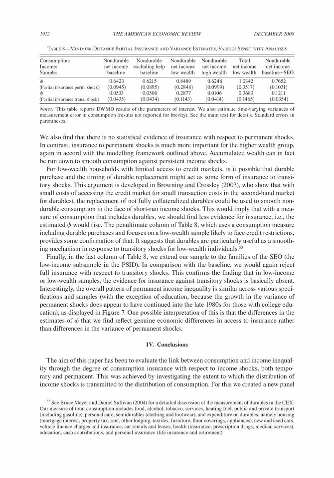
DECEmBER 20081912 THE AmERICAN ECONOmIC REVIEW
We also find that there is no statistical evidence of insurance with respect to permanent shocks. In contrast, insurance to permanent shocks is much more important for the higher wealth group, again in accord with the modelling framework outlined above. Accumulated wealth can in fact be run down to smooth consumption against persistent income shocks.
For low-wealth households with limited access to credit markets, is it possible that durable purchase and the timing of durable replacement might act as some form of insurance to transi-tory shocks. This argument is developed in Browning and Crossley (2003), who show that with small costs of accessing the credit market (or small transaction costs in the second-hand market for durables), the replacement of not fully collateralized durables could be used to smooth non-durable consumption in the face of short-run income shocks. This would imply that with a mea-sure of consumption that includes durables, we should find less evidence for insurance, i.e., the estimated c would rise. The penultimate column of Table 8, which uses a consumption measure including durable purchases and focuses on a low-wealth sample likely to face credit restrictions, provides some confirmation of that. It suggests that durables are particularly useful as a smooth-ing mechanism in response to transitory shocks for low-wealth individuals.35
Finally, in the last column of Table 8, we extend our sample to the families of the SEO (the low-income subsample in the PSID). In comparison with the baseline, we would again reject full insurance with respect to transitory shocks. This confirms the finding that in low-income or low-wealth samples, the evidence for insurance against transitory shocks is basically absent. Interestingly, the overall pattern of permanent income inequality is similar across various speci-fications and samples (with the exception of education, because the growth in the variance of permanent shocks does appear to have continued into the late 1980s for those with college edu-cation), as displayed in Figure 7. One possible interpretation of this is that the differences in the estimates of f that we find reflect genuine economic differences in access to insurance rather than differences in the variance of permanent shocks.
IV. Conclusions
The aim of this paper has been to evaluate the link between consumption and income inequal-ity through the degree of consumption insurance with respect to income shocks, both tempo-rary and permanent. This was achieved by investigating the extent to which the distribution of income shocks is transmitted to the distribution of consumption. For this we created a new panel
35 See Bruce Meyer and Daniel Sullivan (2004) for a detailed discussion of the measurement of durables in the CEX. Our measure of total consumption includes food, alcohol, tobacco, services, heating fuel, public and private transport (including gasoline), personal care, semidurables (clothing and footwear), and expenditure on durables, namely housing (mortgage interest, property tax, rent, other lodging, textiles, furniture, floor coverings, appliances), new and used cars, vehicle finance charges and insurance, car rentals and leases, health (insurance, prescription drugs, medical services), education, cash contributions, and personal insurance (life insurance and retirement).
Table 8—Minimum-Distance Partial Insurance and Variance Estimates, Various Sensitivity Analyses
Consumption: Nondurable Nondurable Nondurable Nondurable Total NondurableIncome: net income excluding help net income net income net income net incomeSample: baseline baseline low wealth high wealth low wealth baseline1SEO
f 0.6423 0.6215 0.8489 0.6248 1.0342 0.76521Partial insurance perm. shock2 10.09452 10.08952 10.28482 10.09992 10.35172 10.10312c 0.0533 0.0500 0.2877 0.0106 0.3683 0.12111Partial insurance trans. shock 2 10.04352 10.04342 10.11432 10.04142 10.14652 10.03542Notes: This table reports DWMD results of the parameters of interest. We also estimate time-varying variances of measurement error in consumption (results not reported for brevity). See the main text for details. Standard errors in parentheses.

VOL. 98 NO. 5 1913BLuNDELL ET AL.: CONSumPTION INEquALITy AND PARTIAL INSuRANCE
consumption series for the PSID using an imputation procedure that maps food data into consump-tion data using the estimates of a demand equation for food, estimated from repeated CEX cross sections. We document a disjuncture between income and consumption inequality that occurred in the middle of the 1980s in the United States. We argue that this disjuncture can be explained by the change in the persistence of income shocks over this period, in particular, an initial growth in permanent shocks, which was then replaced by growth in transitory income shocks.
The analysis uncovers a strong growth in permanent income shocks in the United States dur-ing the early 1980s (the variance of transitory shock also increases, but at a later stage). From trough to peak the variance of the permanent shock doubles, while the variance of the transitory shock goes up by only about 50 percent. The variance of permanent shocks levels off in the sec-ond half of the 1980s. The variance of the transitory shock is only mildly increasing in the period where the variance of permanent shock is increasing, and it increases only when the variance of permanent shock slows down. Although we find important differences in the degree of insur-ance to these shocks by wealth, education, and birth cohort, the interpretation of the relationship between consumption and income inequality is maintained.
The economic framework in this paper allowed for self-insurance, in which consumers smooth idiosyncratic shocks through saving, and complete markets in which all idiosyncratic shocks are insured. Neither of these models was found to accord with the evidence. Instead, we find some partial insurance for permanent shocks and almost complete insurance of transitory shocks. Only for low-wealth households do we find significant sensitivity, and therefore only partial insurance, with respect to transitory income shocks. Interestingly, there appears to be a much greater degree of insurance of permanent shocks among the college educated. Not surprisingly, we also find more insurance of such shocks for older cohorts. Our model suggests that we should see more insurance, even for permanent shocks, among those nearing retirement, especially where they have built up sufficient precautionary savings. The tax and welfare system are also found to play
00.
010.
020.
030.
04B
asel
ine
sam
ple
1980 1982 1984 1986 1988 1990Year
00.
010.
020.
030.
04
1980 1982 1984 1986 1988 1990Year
No college education College education0
0.01
0.02
0.03
0.04
1980 1982 1984 1986 1988 1990Year
Baseline sample Adding SEO
00.
010.
020.
030.
04
1980 1982 1984 1986 1988 1990Year
Baseline sample Total exp.
Figure 7. Variance of Permanent Shocks in Various Specifications and Samples

DECEmBER 20081914 THE AmERICAN ECONOmIC REVIEW
an important insurance role for permanent shocks. When we include durables in our measure of consumption, we find much less evidence of insurance of transitory shocks, suggesting that durables may be acting as an alternative smoothing mechanism for low-wealth families.
Recent work on income and consumption dynamics, building on the earlier studies of earn-ings dynamics by Lee Lillard and Yoram Weiss (1979) and Michael Baker (1997), focuses on models that allow general heterogeneous lifetime income profiles (Guvenen 2006). These studies also find lower overall persistence. As we have noted, the unit root assumption follows findings from many papers in the literature on labor earnings, but alternative processes with less persis-tence and individual trends are increasingly common. The introduction of heterogeneous income trends is an important development and it would be a very useful exercise to extend the model of partial insurance we develop here to such alternative income processes.36 The main point in this study, however, is that it is the change in the degree of persistence of income shocks in the 1980s, rather than the level itself, that explains the observed disjuncture between the evolution of income and consumption inequality.
These results have implications for both macroeconomics and labor economics. The macroeco-nomics literature has long been concerned with explaining why modern economies depart from the complete markets benchmark. Recent work has examined the role of asymmetric information, moral hazard, heterogeneity, etc., and asked whether the complete markets model can be amended to include some form of imperfect insurance. This issue has not been subject to a systematic empir-ical investigation. Insofar as lack of smoothing opportunities implies a greater vulnerability to income shocks, our research can be relevant to issues of the incidence and permanence of poverty studied in the labor economics literature. Studying how well families smooth income shocks, how this changes over time in response to changes in the economic environment confronted, and how different household types differ in their smoothing opportunities is an important complement to understanding the effect of redistributive policies and antipoverty strategies.
Appendix A: Data
The PSID.—The PSID started in 1968 collecting information on a sample of roughly 5,000 households. Of these, about 3,000 were representative of the US population as a whole (the core sample), and about 2,000 were low-income families (the Census Bureau’s Survey of Economic Opportunities, or SEO sample). Thereafter, both the original families and their split-offs (chil-dren of the original family forming a family of their own) have been followed. For most of the analysis we exclude SEO households and their split-offs. However, we do consider the robustness of our results in the low income SEO subsample.37
The PSID includes a variety of socioeconomic characteristics of the household, including education, food spending, and income of household members. Questions referring to income are retrospective; thus, those asked in 1993, say, refer to the 1992 calendar year. In contrast, the tim-ing of the survey questions on food expenditure is much less clear (see Hall and Mishkin 1982, and Altonji and Siow 1987, for two alternative views). Typically, the PSID asks how much is spent on food in an average week. Since interviews are usually conducted around March, it has been argued that people report their food expenditure for an average week around that period, rather than for the previous calendar year as is the case for family income. We assume that food expenditure reported in survey year t refers to the previous calendar year, but check the effect of alternative assumptions.
36 Baker and Gary Solon (2003) use a large Canadian tax administrative dataset to show that the random walk com-ponent remains of key importance even in the heterogeneous trends specification.
37 See Martha Hill (1992) for more details about the PSID.

VOL. 98 NO. 5 1915BLuNDELL ET AL.: CONSumPTION INEquALITy AND PARTIAL INSuRANCE
Households in the PSID report their taxable family income (which includes transfers and financial income). The measure of income used in the baseline analysis below excludes income from financial assets, subtracts federal taxes on nonfinancial income and deflates the corre-sponding value by the CPI. We assume that federal taxes on nonfinancial income are a propor-tion of total federal taxes given by the ratio between nonfinancial income and total income. We consider two education groups: with and without college education (corresponding to more than high school and high school or less, respectively).
Since CEX data are available on a consistent basis since 1980, we construct an unbalanced PSID panel using data from 1978 to 1992 (the first two years are retained for initial conditions purposes). Due to attrition, changes in family composition, and various other reasons, household heads in the 1978–1992 PSID may be present from a minimum of one year to a maximum of fifteen years. We thus create unbalanced panel datasets of various length. The longest panel includes individu-als present from 1978 to 1992; the shortest, individuals present for two consecutive years only (1978–79, 1979–80, up to 1991–92).
The objective of our sample selection is to focus on a sample of continuously married couples headed by a male (with or without children). We eliminate households facing some dramatic family composition change over the sample period. In particular, we keep only those with no change, and those experiencing changes in members other than the head or the wife (children leaving parental home, say). We next eliminate households headed by a female and those with missing report on race, education, and region. We keep continuously married couples and drop some income outliers.38 We then drop those born before 1920 or after 1959. Finally, we drop those under the age of 30 and older than 65. This is to avoid problems related to changes in fam-ily composition and education, in the first case, and retirement, in the second.39 The final sample used in the minimum distance exercise below is composed of 17,604 observations and 1,765 households. Our income regressions do not use 36 observations with topcoded income, financial income, or federal taxes.
The CEX.—The Consumer Expenditure Survey provides a continuous and comprehensive flow of data on the buying habits of American consumers. The data are collected by the Bureau of Labor Statistics and used primarily for revising the CPI.40 The definition of the head of the household in the CEX is the person or one of the persons who owns or rents the unit; this defini-tion is slightly different from the one adopted in the PSID, where the head is always the husband in a couple. We make the two definitions compatible.
The CEX is based on two components, the Diary survey and the Interview survey. The Diary sample interviews households for two consecutive weeks, and it is designed to obtain detailed expenditures data on small and frequently purchased items. The Interview sample follows survey households for a maximum of five quarters, although only inventory and basic sample data are collected in the first quarter. The data base covers about 95 percent of all expenditure. Following most previous research, our analysis below uses only the Interview sample.41
38 An income outlier is defined as a household with an income growth above 500 percent, below 280 percent, or with a level of income below $100 in a given year.
39 More details on variable construction and step-by-step selection of our PSID and CEX samples is available in the full Web Appendix on the AER Web site.
40 A description of the survey, including more details on sample design, interview procedures, etc., may be found in “Chapter 16: Consumer Expenditures and Income,” from the BLS Handbook of methods.
41 There is some evidence that trends in consumption inequality measured in the two CEX surveys have diverged in the 1990s (Attanasio, Battistin, and Ichimura 2004). While research on the reasons for this divergence is clearly war-ranted, our analysis, which uses data up to 1992, will be only marginally affected.

DECEmBER 20081916 THE AmERICAN ECONOmIC REVIEW
As the PSID, the CEX collects information on a variety of sociodemographic variables, includ-ing income and consumer expenditure. Expenditure is reported in each quarter and refers to the previous quarter; income is reported in the second and fifth interview (with some exceptions), and refers to the previous 12 months. For consistency with the timing of consumption, fifth-quarter income data are used.
Our initial 1980–2004 CEX sample includes 1,848,348 monthly observations, corresponding to 192,564 households. We drop those with missing records on food and/or zero total nondurable expenditure, and those that completed fewer than 12 month interviews. This is to obtain a sample where a measure of annual consumption can be obtained. We then sum food at home, food away from home, and other nondurable expenditures over the 12 interview months. This gives annual expenditures. For consistency with the timing of the PSID data, we drop households interviewed after 1992. We also drop those with zero before-tax income, those with missing region or educa-tion records, single households, and those with changes in family composition. Finally, we elimi-nate households where the head is born before 1920 or after 1959, persons younger than 30 or older than 65, and those with outlier income (defined as a level of income below the amount spent on food) or incomplete income responses. The final sample used to estimate the food demand equation in Table 1 contains 14,430 households.
Appendix B: The Euler Equation Approximation
If preferences are quadratic (and interest rates are not subject to uncertainty), it is possible to obtain a closed-form solution for consumption. It is also straightforward to derive an exact map-ping between the expectation error of the Euler equation for consumption and income shocks. See Hall and Mishkin (1982), for example. Quadratic preferences have well-known undesirable features, such as increasing risk aversion and lack of a precautionary motive for saving. More realistic preferences, such as the CRRA functional form used here, solve these problems but deliver no closed-form solution for consumption. The Euler equation in the CRRA case can be linearized to describe the behavior of consumption growth and to derive an approximation of the mapping between the expectation error of the Euler equation and the income shock. We refer the interested reader to the full Web Appendix (available on the AER Web site) for complete details on how we can obtain the approximated Euler equation (3) in the self-insurance case.
Appendix C: Identification
Here we show how the model can be identified with four years of data (t 1 1, t, t 2 1, t 2 2). We start with the simplest model with no measurement error, serially uncorrelated transitory component, and stationarity. For simplicity we omit the individual subscripts.
The Simplest model.—(Unexplained) consumption and income growth in period s (s 5 t 2 1, t, t 1 1) are, respectively:
Dcs 5 js 1 fzs 1 ces,
Dys 5 zs 1 Des,
(where, for simplicity, we have assumed that the transitory shock to income is i.i.d.).42 The param-eters to identify are: f, c, sj
2, sz2, and se
2.
42 The proof mechanism can easily be extended to deal with MA(q) transitory shock processes as in Meghir and Pistaferri (2004).

VOL. 98 NO. 5 1917BLuNDELL ET AL.: CONSumPTION INEquALITy AND PARTIAL INSuRANCE
As in Meghir and Pistaferri (2004), we can prove that
(C1) E 1Dyt 1Dyt21 1 Dyt 1 Dyt112 2 5 sz2
and that
(C2) E 1DytDyt212 5 E 1Dyt11 Dyt 2 5 2se2.
Identification of se2 through (C2) rests on the idea that income growth rates are autocorrelated
due to mean reversion caused by the transitory component (the permanent component is subject to i.i.d. shocks). Identification of sz
2 through (C1) rests on the idea that the variance of income growth (E 1DytDyt 2 ) coincides with the variance of innovations to the permanent component, after removing the contribution of the mean reverting component (E 1DytDyt212 1 E 1Dyt Dyt112).
In general, if one has T years of data, only T 2 3 variances of the permanent shock can be identified, and only T 2 2 variances of the i.i.d. transitory shock can be identified. As said in the text, with panel data on income, the variances of permanent and transitory shock can be identi-fied without recourse to consumption data.
One can also prove that
E 1Dct 1Dyt21 1 Dyt 1 Dyt 2 2(C3) 5 f, E 1Dyt 1Dyt21 1 Dyt 1 Dyt 2 2
E 1Dct Dyt112(C4) 5 c, E 1DytDyt112
3E 1Dct 1Dyt21 1 Dyt 1 Dyt112 2 42 3E 1Dct Dyt112 42(C5) E 1Dct 1Dct21 1 Dct 1 Dct112 2 2 1 5 sj2.
E 1Dyt 1Dyt21 1 Dyt 1 Dyt112 2 E 1DytDyt112
These moment conditions provide complete identification of the parameters of interest. Identification of c using (C4) uses the fact that income and lagged consumption may be cor-related through the transitory component 1E 1DctDyt112 5 cse
22 . Scaling this by E 1DytDyt112 5 se
2 identifies the loading factor c. Note that there is a simple IV interpretation here: c is identi-fied by a regression of Dct on Dyt using Dyt11 as an instrument. A similar reasoning applies to (C3): the current covariance between consumption and income growth 1E 1DctDyt 2 2 , stripped of the contribution of the transitory component, reflects the arrival of permanent income shocks 1E 1Dct 1Dyt21 1 Dyt 1 Dyt 2 2 5 fsz
22 . Scaling this by the variance of permanent income shock, identified by using income moments alone, identifies the loading factor f. Note that here, too, there is a simple IV interpretation: f is identified by a regression of Dct on Dyt using 1Dyt21 1 Dyt 1 Dyt112 as an instrument. Finally, (C5) identifies the variance of the component sj
2 using a residual variability idea: the variance of consumption growth, stripped of the contribution of permanent and transitory income shocks, reflects heterogeneity in the consumption gradient.
The full Web Appendix discusses identification under a number of alternative scenarios: (a) measurement error in consumption, (b) measurement error in income, (c) non-stationarity, and (d) more general models in which consumption depends on current and lagged income shocks.

DECEmBER 20081918 THE AmERICAN ECONOmIC REVIEW
Appendix D: Estimation Details
The two basic vectors of interest are
Dci, 1 Dyi, 1
Dci, 2 Dyi, 2
Dci 5 ± … ≤ and Dyi 5 ± … ≤
,
Dci, T Dyi, T
where, for simplicity, we indicate with 0 the first year in the panel (1978) and with T the last (1992), and the reference to age has been omitted. Since PSID consumption data were not col-lected in 1987 and 1988, the vector Dci is understood to have dim 1Dyi 2 2 3, i.e., the rows with missing consumption data have already been sweeped out from Dci. Moreover, if the individual was not interviewed in year t, we replace the unobservable Dci, t and Dyi, t with zeros. Conformably with the vectors above, we define
dci, 1 dy
i, 1
dci, 2 dy
i, 2
di
c 5 ± … ≤ and diy 5 ± … ≤ ,
dci, T dy
i, T
where dci, t 5 15Dci, t is not missing6 and dy
i, t 5 15Dyi, t is not missing6. Overall, this notation allows us to handle in a simple manner the problems of unbalanced panel data and of missing consump-tion data in 1987 and 1988.
Stacking observations on Dy and Dc (and on dc and dy) for each individual, we obtain the vectors
Dci dic
xi 5 q r and di 5 q r . Dyi dy
i
Now we can derive
N N
m 5 vech u q a xi xi9r ⊘ q a di di9r v , i51 i51
where ⊘ denotes an elementwise division. The vector m contains the estimates of cov 1Dyt, Dyt1s 2 , cov 1Dyt, Dct1s2 , and cov 1Dct, Dct1s2 , a total of T 12T 1 12 unique moments.43 To obtain the variance-covariance matrix of m, define conformably with m the individual vector, mi 5 vech 5xi xi96.
The variance-covariance matrix of m that can be used for inference is
N N
V 5 s a 1 1mi 2 m 2 1mi 2 m 292 sp 1Di Di92 t ⊘ q a Di Di9r , i51 i51
where Di 5 vech 5di di96 and sp denotes an elementwise product. The square roots of the elements in the main diagonal of V provide the standard errors of the corresponding elements in m.
What we do in the empirical analysis is to estimate models for m:
43 In practice there are fewer than T 12T 1 12 moments because data on consumption are not available all years.
VOL. 98 NO. 5 1919BLuNDELL ET AL.: CONSumPTION INEquALITy AND PARTIAL INSuRANCE
m 5 f 1L2 1 Y ,
where Y captures sampling variability and L is the vector of parameters we are interested in (the variances of the permanent shock and the transitory shock, the partial insurance parameters, etc.). We solve the problem of estimating L by minimizing
min 1m 2 f 1L2 29A1m 2 f 1L2 2 , L
where A is a weighting matrix. Optimal minimum distance (OMD) imposes A 5 V21, equally weighted minimum distance (EWMD) imposes A 5 I, and diagonally weighted minimum dis-tance (DWMD) requires that A is a diagonal matrix with the elements in the main diagonal given by diag 1V212 .
For inference purposes we require the computation of standard errors. Gary Chamberlain (1984) shows that these can be obtained as
`
var 1L̂2 5 1G9AG221G9AVAG 1G9AG221,
where G 5 0f 1L2/0L Z L5L̂ is the Jacobian matrix evaluated at the estimated parameters L̂.
REFERENCES
Abowd, John M., and David Card. 1989. “On the Covariance Structure of Earnings and Hours Changes.” Econometrica, 57(2): 411–45.
Altonji, Joseph G., Ana Paula Martins, and Aloysius Siow. 2002. “Dynamic Factor Models of Consump-tion, Hours and Income.” Research in Economics, 56(1): 3–59.
Altonji, Joseph G., and Lewis M. Segal. 1996. “Small-Sample Bias in GMM Estimation of Covariance Structures.” Journal of Business and Economic Statistics, 14(3): 353–66.
Altonji, Joseph G., and Aloysius Siow. 1987. “Testing the Response of Consumption to Income Changes with (Noisy) Panel Data.” quarterly Journal of Economics, 102(2): 293–328.
Alvarez, Fernando, and Urban J. Jermann. 2000. “Efficiency, Equilibrium, and Asset Pricing with Risk of Default.” Econometrica, 68(4): 775–97.
Attanasio, Orazio, Erich Battistin, and Hidehiko Ichimura. 2004. “What Really Happened to Consump-tion Inequality in the US?” National Bureau of Economic Research Working Paper 10338.
Attanasio, Orazio, and Steven J. Davis. 1996. “Relative Wage Movements and the Distribution of Con-sumption.” Journal of Political Economy, 104(6): 1227–62.
Attanasio, Orazio, and Nicola Pavoni. 2006. “Risk Sharing in Private Information Models with Asset Accumulation: Explaining the Excess Smoothness of Consumption.” Unpublished.
Attanasio, Orazio, and José Víctor Ríos Rull. 2000. “Consumption Smoothing in Island Economies: Can Public Insurance Reduce Welfare?” European Economic Review, 44(7): 1225–58.
Attanasio, Orazio, and Guglielmo Weber. 1995. “Is Consumption Growth Consistent with Intertempo-ral Optimization? Evidence from the Consumer Expenditure Survey.” Journal of Political Economy, 103(6): 1121–57.
Auerbach, Alan J., and Daniel Feenberg. 2000. “The Significance of Federal Taxes as Automatic Stabiliz-ers.” Journal of Economic Perspectives, 14(3): 37–56.
Baker, Michael. 1997. “Growth-Rate Heterogeneity and the Covariance Structure of Life-Cycle Earnings.” Journal of Labor Economics, 15(2): 338–75.
Baker, Michael, and Gary Solon. 2003. “Earnings Dynamics and Inequality among Canadian Men, 1976–1992: Evidence from Longitudinal Income Tax Records.” Journal of Labor Economics, 21(2): 289–321.
Blundell, Richard, Hamish Low, and Ian Preston. 2007. “Income Risk and Consumption Inequality: A Simulation Study.” Institute for Fiscal Studies Working Paper 04/26 (revised November 2007).

DECEmBER 20081920 THE AmERICAN ECONOmIC REVIEW
Blundell, Richard, and Luigi Pistaferri. 2003. “Income Volatility and Household Consumption: The Impact of Food Assistance Programs.” Journal of Human Resources, 38(S): 1032–50.
Blundell, Richard, Luigi Pistaferri, and Ian Preston. 2004. “Imputing Consumption in the PSID Using Food Demand Estimates from the CEX.” Institute for Fiscal Studies Working Paper 04/27.
Blundell, Richard, and Ian Preston. 1998. “Consumption Inequality and Income Uncertainty.” quarterly Journal of Economics, 113(2): 603–40.
Browning, Martin, and Thomas Crossley. 2003. “Shocks, Stocks and Socks: Consumption Smoothing and the Replacement of Durables.” Unpublished.
Caballero, Ricardo J. 1990. “Consumption Puzzles and Precautionary Savings.” Journal of monetary Economics, 25(1): 113–36.
Campbell, John Y., and Angus Deaton. 1989. “Why Is Consumption So Smooth?” Review of Economic Studies, 56(3): 357–73.
Carroll, Christopher D. 2001. “Precautionary Saving and the Marginal Propensity to Consume out of Per-manent Income.” National Bureau of Economic Research Working Paper 8233.
Chamberlain, Gary. 1984. “Panel Data.” In Handbook of Econometrics, Vol. 2, ed. Zvi Griliches and Michael D. Intriligator, 1247–1318. Amsterdam: North-Holland.
Cunha, Flavio, James Heckman, and Salvador Navarro. 2005. “Separating Uncertainty from Heterogene-ity in Life Cycle Earnings.” Oxford Economic Papers, 57(2): 191–261.
Cutler, David M., and Lawrence F. Katz. 1992. “Rising Inequality? Changes in the Distribution of Income and Consumption in the 1980s.” American Economic Review, 82(2): 546–51.
Deaton, Angus. 1992. understanding Consumption. Oxford: Oxford University Press.Deaton, Angus. 1997. The Analysis of Household Surveys: A microeconometric Approach to Development
Policy. Baltimore: Johns Hopkins University Press.Deaton, Angus, and Christina Paxson. 1994. “Intertemporal Choice and Inequality.” Journal of Political
Economy, 102(3): 437–67.Dynarski, Susan, and Jonathan Gruber. 1997. “Can Families Smooth Variable Earnings?” In Brookings
Papers on Economic Activity, Vol. 1, ed. William C. Brainard and George L. Perry, 229–305. Washing-ton, DC: Brookings Institution Press.
Engen, Eric M., and Jonathan Gruber. 2001. “Unemployment Insurance and Precautionary Saving.” Jour-nal of monetary Economics, 47(3): 545–79.
Fay, Scott, Erik Hurst, and Michelle J. White. 2002. “The Household Bankruptcy Decision.” American Economic Review, 92(3): 706–18.
Flavin, Marjorie A. 1981. “The Adjustment of Consumption to Changing Expectations about Future Income.” Journal of Political Economy, 89(5): 974–1009.
Gruber, Jonathan. 2000. “Cash Welfare as a Consumption Smoothing Mechanism for Divorced Mothers.” Journal of Public Economics, 75(2): 157–82.
Gruber, Jonathan, and Aaron Yelowitz. 1999. “Public Health Insurance and Private Savings.” Journal of Political Economy, 107(6): 1249–74.
Guiso, Luigi, Luigi Pistaferri, and Fabiano Schivardi. 2005. “Insurance within the Firm.” Journal of Political Economy, 113(5): 1054–87.
Guvenen, Fatih. 2007. “Learning Your Earning: Are Labor Income Shocks Really Very Persistent?” Amer-ican Economic Review, 97(3): 687–712.
Hall, Robert E., and Frederic S. Mishkin. 1982. “The Sensitivity of Consumption to Transitory Income: Estimates from Panel Data on Households.” Econometrica, 50(2): 461–81.
Hayashi, Fumio, Joseph Altonji, and Laurence Kotlikoff. 1996. “Risk-Sharing between and within Fami-lies.” Econometrica, 64(2): 261–94.
Heathcote, Jonathan, Kjetil Storesletten, and Giovanni L. Violante. 2004. “The Macroeconomic Impli-cations of Rising Wage Inequality in the United States.” Centre for Economic Policy Research Discus-sion Paper 4296.
Heathcote, Jonathan, Kjetil Storesletten, and Giovanni L. Violante. 2007. “Consumption and Labour Sup-ply with Partial Insurance: An Analytical Framework.” Centre for Economic Policy Research Discus-sion Paper 6280.
Hill, Martha. 1992. The Panel Study of Income Dynamics: A user’s Guide. Newbury Park, California: Sage Publications.
Johnson, David S., and Timothy M. Smeeding. 1998. “Measuring the Trends in Inequality of Individuals and Families: Income and Consumption.” Unpublished.
Johnson, David S., Timothy M. Smeeding, and Barbara Boyle Torrey. 2005. “Economic Inequality through the Prisms of Income and Consumption.” monthly Labor Review, 128(4): 11–24.

VOL. 98 NO. 5 1921BLuNDELL ET AL.: CONSumPTION INEquALITy AND PARTIAL INSuRANCE
Kimball, Miles S., and N. Gregory Mankiw. 1989. “Precautionary Saving and the Timing of Taxes.” Jour-nal of Political Economy, 97(4): 863–79.
Kniesner, Thomas J., and James P. Ziliak. 2002. “Tax Reform and Automatic Stabilization.” American Economic Review, 92(3): 590–612.
Kotlikoff, Laurence J., and Avia Spivak. 1981. “The Family as an Incomplete Annuities Market.” Journal of Political Economy, 89(2): 372–91.
Krueger, Dirk, and Fabrizio Perri. 2006. “Does Income Inequality Lead to Consumption Inequality? Evi-dence and Theory.” Review of Economic Studies, 73(1): 163–93.
Lillard, Lee A., and Yoram Weiss. 1979. “Components of Variation in Panel Earnings Data: American Sci-entists, 1960–70.” Econometrica, 47(2): 437–54.
MaCurdy, Thomas E. 1982. “The Use of Time Series Processes to Model the Error Structure of Earnings in a Longitudinal Data Analysis.” Journal of Econometrics, 18(1): 83–114.
Meghir, Costas, and Luigi Pistaferri. 2004. “Income Variance Dynamics and Heterogeneity.” Economet-rica, 72(1): 1–32.
Meyer, Bruce D., and James X. Sullivan. 2004. “The Effects of Welfare and Tax Reform: The Material Well-Being of Single Mothers in the 1980s and 1990s.” Journal of Public Economics, 88 (7–8): 1387–1420.
Moffitt, Robert A. 1997. “Comment on ‘Can Families Smooth Variable Earnings.’” In Brookings Papers on Economic Activity, Vol. 1, ed. William C. Brainard and George L. Perry, 285–92. Washington, DC: Brookings Institution Press.
Moffitt, Robert A., and Peter Gottschalk. 1995. “Trends in the Covariance Structure of Earnings in the US: 1969–1987.” University of Wisconsin Institute for Research on Poverty Discussion Paper 1001–93.
Moffitt, Robert A., and Peter Gottschalk. 2002. “Trends in the Transitory Variance of Earnings in the United States.” Economic Journal, 112(478): C68–73.
Primiceri, Giorgio, and Thijs van Rens. Forthcoming. “Heterogeneous Life-Cycle Profiles, Income Risk and Consumption Inequality.” Journal of monetary Economics.
Skinner, Jonathan. 1987. “A Superior Measure of Consumption from the Panel Study of Income Dynam-ics.” Economic Letters, 23(2): 213–16.
Slesnick, Daniel T. 2001. Consumption and Social Welfare: Living Standards and Their Distribution in the united States: Cambridge, UK: Cambridge University Press.
Stephens, Melvin, Jr. 2001. “The Long-Run Consumption Effects of Earnings Shocks.” Review of Eco-nomics and Statistics, 83(1): 28–36.
Stephens, Melvin, Jr. 2002. “Worker Displacement and the Added Worker Effect.” Journal of Labor Eco-nomics, 20(3): 504–37.
Ziliak, James P. 1998. “Does the Choice of Consumption Measure Matter? An Application to the Perma-nent-Income Hypothesis.” Journal of monetary Economics, 41(1): 201–16.