Comments invited.

Version 9.0

Consumption-Based Asset Pricing:

Research and Applications

By

Douglas T. Breeden,* Robert H. Litzenberger,**

and Tingyan Jia***

Current version: October 27, 2014

*William W. Priest Professor of Finance, Fuqua School of Business, Duke University.

Contact: doug.breeden@duke.edu

**Edward Hopkinson Professor of Investment Banking Emeritus, The Wharton School, University of

Pennsylvania.

***Guanghua School of Management, Peking University, and Visiting Scholar, Duke University

Fuqua School of Business. Contact: jiatingyan2011@gmail.com

We thank Ravi Bansal, Alon Brav, John Campbell, Campbell Harvey, Sydney Ludvigson and

especially Dana Kiku for helpful comments and materials.

1

Abstract

This article reviews the origins and development of the consumption-based asset pricing theory

over the last four decades. Starting with the original CCAPM derivations by Rubinstein (1976),

Breeden-Litzenberger (1978) and Breeden (1979), as well as related work by Lucas (1978), both

theory and subsequent tests are reviewed, and some new applications are provided. While initial

empirical tests such as those of Hansen-Singleton (1983) and Mehra-Prescott (1985) were largely

negative, more recent tests are much more supportive of CCAPM theory. Empirical tests from

several authors are presented, including those of Lettau-Ludvigson (2001), who use a

consumption/wealth conditioning variable, Parker-Julliard (2005) who examine “ultimate

consumption betas,” and Jagannathan-Wang (2007) who examine intra-year decision making

effects on tests. Important second generation consumption-based asset pricing advances of

Campbell and Cochrane (1999) on external habit formation and Bansal and Yaron (2004) on

long-run risk are also reviewed. These models develop utility functions that are consistent with

both large cyclical changes in relative risk aversion and risk premiums, and lagged impacts of

aggregate consumption changes on risk premiums. These second generation models have many

free parameters and are able to fit the empirical data much better than the first generation

CCAPM models.

2

I. Introduction.

Consumption-based asset pricing models have been among the leading multiperiod

general equilibrium asset pricing models in financial economics research for the past 35 years.

The Consumption Capital Asset Pricing Model (CCAPM) was first derived in the late 1970s in

successively more general models by Rubinstein (1976), Breeden and Litzenberger (1978), and

Breeden (1979).1 While Lucas (1978) did not derive the CCAPM formula, his work on Euler

equations was also helpful to many empiricists in subsequent consumption-based asset pricing

tests. The CCAPM built on the classic single-period, market-based CAPM of Sharpe (1964) and

Lintner (1965), as well as on the subsequent major work on the Intertemporal CAPM by Merton

(1973). The Consumption CAPM links asset pricing with macroeconomic risk.

The CCAPM states that the expected excess return on any risky asset should be

proportional to its “consumption beta.” These authors showed that securities with higher

sensitivities of returns to movements in real consumption spending have more systematic risk

and should have proportionately higher excess returns. They pay off more when consumption is

high and marginal utility is low, and pay less when consumption is low and marginal utility is

high, so they are worth less in price and have higher equilibrium returns. This is different from

the original market-oriented CAPM insights of Sharpe (1964) and Lintner (1965), as real

consumption growth is not perfectly correlated with market returns. In a multiperiod model,

market wealth can be high and still have marginal utility be high if the investment opportunity

set is good, as shown by Merton (1973) and Breeden (1984).

1See p. 412 of Rubinstein (1976) , eqs. 26 and 27 in Breeden-Litzenberger (1978) and

eqs. 19, 19’, and 35 in Breeden (1979) for the first CCAPM equations. Lucas’s (1978) important

paper has also been credited with CCAPM development, but the paper has no equations with

consumption covariances or consumption betas and no CCAPM asset pricing formula. Lucas’s

development of the relation of asset prices to marginal utility is similar in economic intuition to

the time-state preference literature of Hirshleifer (1970, Chapter 8), Rubinstein (1974, 1976), and

Nielsen (1974). We view Lucas’s most important contributions to be on the existence and

stability of equilibrium and of an equilibrium pricing density with intuitive economic properties.

3

The first two decades of CCAPM tests produced mixed results. Tests of the special case

of the CCAPM under constant relative risk aversion by Hansen and Singleton (1983), Mehra and

Prescott (1985) and others rejected the model. Chen, Roll and Ross (1986) found no significant

consumption factor priced when in the presence of other factors, including industrial production,

junk bond returns, and inflation hedges. Grossman, Melino and Shiller (1987), Breeden,

Gibbons and Litzenberger (BGL, 1989) and Wheatley (1988) examined measurement issues in

consumption (such as time aggregation) and their biases on measures of volatility and

consumption betas. BGL found a significant positive coefficient on consumption betas; and

separately a significant positive coefficient on market betas; however, both the CCAPM and the

CAPM were rejected based on stronger form tests of their respective implied first order

conditions. BGL derived two useful results used by several subsequent authors: (1) biases in

consumption betas due to time aggregation and how those biases are reduced with increased

differencing intervals for consumption growth and (2) estimation of consumption betas relative

to returns on a consumption mimicking portfolio, which allows greater number and frequency of

observations and more precise estimates of consumption betas.

The very strong theory in support of the CCAPM, contrasted with weak early empirical

support, motivated researchers to improve both their theoretical and empirical modeling. On the

theoretical side, Pye (1972, 1973) and Greenig (1986) developed time-multiplicative utility

functions, and then Sundaresan (1989), Constantinides (1990) and Abel (1990) modeled habit

formation and then Epstein-Zin (1989) and Weil (1989) (often jointly referred to as EZ-W)

developed preference structures that displayed time-complementarity in utility for consumption

streams, allowing researchers to separate effects of different levels of intratemporal relative risk

aversion (RRA) from levels of the elasticity of intertemporal substitution (EIS). Campbell and

Cochrane (1999) later produced an empirically tractable model with the habit formation

approach, using an “external habit.” With a subsistence level of consumption for a

“representative individual,” their model allows for dramatic rises in relative risk aversion as

surplus consumption (above habit) goes towards zero in severe recessions. With the flexibility

afforded by this model, they were able to fit many aspects of empirical data on stock and bond

returns as related to real consumption growth, especially the risk premium on the stock market,

4

which Mehra and Prescott (1985) had found was substantially too high (the “equity premium

puzzle”), given the low volatility of real consumption growth.

In the early 1990s, Mankiw and Zeldes (1991) considered that many households did not

own stock at all or in significant amounts, a situation called “limited participation.” They

pointed out that there is no reason that the Euler equation should hold for households who are not

investing. They found that for households who actually owned stocks, the implied estimates of

relative risk aversion were much more reasonable than for households who did not own stocks.

Heaton and Lucas (1992, 1996) examined “incomplete markets” that did not permit full hedging

of labor income, thus causing consumers to have more volatile consumption streams. Brav,

Constantinides and Geczy (2002) studied consumer spending data and found generally plausible

estimates of relative risk aversion, given the high volatilities of individuals’ consumption

streams. Vissing-Jorgensen (2002) focused on estimating the “elasticity of intertemporal

substitution,” which determines how much consumers change their expected consumption

growth rate when interest rates or expected returns on assets change. She finds the EIS to be

quite different for stockholders than for nonstockholders, generally getting plausible estimates

for those who chose to invest in stocks and bonds and based on trading off current consumption

versus future consumption.

Also on the empirical side, advances were also made in examining changes in

conditional means, variances and covariances and testing conditional versions of the CAPM and

CCAPM, as in Harvey (1991), Ferson and Harvey (1991) Jagannathan and Wang (1996), and

Ferson and Harvey (1999). Particularly insightful papers in testing the conditional CCAPM

include Lettau and Ludvigson (2001a, b) and Jagannathan and Wang (2007). Lettau-Ludvigson

use deviations of consumption from total wealth (which includes a human capital estimate in

addition to stock market wealth) as a conditioning or “scaling” variable for changing mean

returns. They find results quite compatible with Merton’s (1973) and Breeden’s (1984)

intertemporal theories, in that high consumption versus wealth is a predictor of future investment

returns, as consumers optimally smooth forward those changes in expected returns. Lettau and

Ludvigson also find significant differences in the movements of consumption betas of value vs.

growth stocks during recessions. They find that value stocks tend to have much larger increases

5

in consumption betas during recessions, when risks and risk premiums are high, which helps to

explain the Fama-French (1992) findings of higher returns on value stocks than predicted by the

unconditional CCAPM betas, results which were viewed as anomalous. Jagannathan and Wang

use recession and expansion periods identified by the NBER as a conditioning variable, and find

that conditional consumption betas are excellent in describing conditional mean returns on the

Fama-French portfolios.

More recently, Bansal and Yaron’s (2004) article has had major impact by modeling the

“long run risk” caused by small, persistent shocks in the drift and volatility of real consumption

growth. They show that variance of real consumption growth grows more than proportionally

with time, which is consistent with the persistence of growth shocks. Additionally, they provide

evidence that shows that the conditional volatility of consumption is time-varying, which leads

naturally to time-varying risk premia. Much subsequent research has been done on this long run

risk model, most notably in the paper by Bansal, Dittmar, and Kiku (2009). Bansal, Dittmar and

Kiku show that aggregate consumption and aggregate dividends have a cointegrating relation.

They observe that “the deviation of the level of dividends from consumption (the error correction

variable) is important for predicting dividend growth rates and returns at all horizons” (1, 5 and

10 years). Imposing cointegration allows them to predict 11.5% of the variation in 1-year

returns, whereas only 7.5% of the variation is predicted without cointegration. Their conditional

consumption betas account for about 75% of the cross-sectional variation in risk premia for the

one-year horizon, and 85% for long horizons.

After Grossman, Melino and Shiller (1987) and Breeden, Gibbons and Litzenberger

(1989) raised concerns about measuring consumption, in 2005 Parker and Julliard showed that it

is important to measure “ultimate consumption betas,” since consumption changes are slow-

moving, and could take 2-3 years for the full effects to be observed. Using measures of these

ultimate consumption betas, they were able to explain much of the Fama-French (1992) effects

for size-related portfolios and value vs. growth (book/market) portfolios.

Jagannathan and Wang (2007) show that when consumption betas of stocks are computed

using year-over-year consumption growth based upon the fourth quarter, the consumption-based

6

CAPM explains the cross-section of stock returns as well as the Fama and French (1992) three-

factor model. Jagannathan-Wang argue that major investment and job decisions are most often

made in the fourth quarter, as investors and firms plan for the coming year, so this is when the

Euler equations should fit best. For estimation of consumption betas, they follow Breeden-

Gibbons-Litzenberger (1989) in using a “consumption mimicking portfolio” (CMP) formed from

the 6 Fama-French benchmark portfolios, using weights from an OLS regression of consumption

growth on the benchmark portfolios. This allows them to substitute synchronous portfolio

returns for (time aggregated) real consumption growth in the empirical tests, giving more

precisely estimated consumption betas.

The plan of the paper is as follows: Section II derives the main theoretical results for

aggregation of consumption in a discrete time-state preference model, and then the CCAPM in

Merton’s continuous-time model. Section III derives the term structure of interest rates from the

term structure of expected growth of consumption, the term structure of volatility and the term

structure of inflation, and then shows tests of this theory. Section IV discusses selected early

1980s tests of the CCAPM and focuses on the equity premium puzzle of Mehra and Prescott,

given its large impact on subsequent research. Section V presents the Breeden, Gibbons,

Litzenberger derivations for time aggregation and the consumption mimicking portfolio. Section

VI presents the advances in modeling utility maximization with non-time-separable utility

function. Section VII discusses significant research on limited participation and incomplete

markets. Section VIII presents the 1990s empirical modeling of changing conditional risks and

changing risk premiums. Section IX discusses the advances in empirical applications of models

with habit formation, led by the Campbell-Cochrane model. Section X presents the 2001-2007

results on modeling changes in conditional consumption risk and changes in the investment and

job opportunity sets, led by Lettau and Ludvigson. Section XI presents the long-run risk model

and tests and developments based on the original work by Bansal and Yaron. Section XII

presents research on cash flow betas (dividends and profits) on real consumption growth versus

market returns. As the consumption-based asset pricing literature is so vast, Section XIII

presents descriptions of additional selected works in the last decade, which has been dominated

by additional extensions and tests of competing empirical models with habit formation, long-run

risk and disaster risk. Section XIV makes some concluding remarks.

7

II. Review of Consumption CAPM Theory.

A. Individuals Are Different. Aggregation of Consumption

In reality, investment counselors know that individuals are often quite different in their

preferences and behavior, having different levels of risk aversion, different tax brackets, and

different preferences with regard to nonlinear risks, such as those causing positive and negative

skewness (i.e., tail risks). Some prefer to lever up to get high returns and are willing to accept

high risks, while others choose to hold a lot of Treasury securities and low return/low risk

combinations. Some are willing to write insurance by taking credit risks or fixed rate mortgage

prepayment risks, while others wish to purchase portfolio insurance, paying a price to limit

downside risk while retaining much of the upside potential. Reactions to alternate possible

consumption paths can also vary quite a lot, as some individuals may be comfortable taking the

risk of having to reduce consumption significantly if markets fall sharply, while others may go to

extreme lengths to smooth consumption or to protect their consumption from going below a

certain subsistence threshold.

Dealing with heterogeneous preferences like these is a challenge analytically to asset pricing

theorists. Papers have been written on the “aggregation problem” and how to allow individuals

to have heterogeneous preferences and yet derive asset pricing results in terms of aggregate

wealth or aggregate consumption. Yet it is surprising that many of the most well-known articles

in consumption-based asset pricing simply assume either identical individuals or the existence of

a “representative individual (e.g. Lucas (1978), Campbell-Cochrane (1999), Bansal-Yaron

(2004)). This may lead students to believe that the aggregation problem is unsolvable and that

we have to just assume it away. That is not true in some important cases, as shown by Merton

(1973), Breeden and Litzenberger (1978) and Breeden (1979), which derive the Intertemporal

CAPM (ICAPM) and the Consumption CAPM (CCAPM) and actually are able to aggregate

fully diverse preferences in the class of time-additive utility functions. It is insightful to show

how market price signals coordinate optimal consumption plans in such a way that legitimate

aggregation results can be obtained.

8

Breeden and Litzenberger (1978, Theorem 1) provide the most general aggregation

theorem that we are aware of to date. We use their basic time-state preference model to derive

the aggregation result. Each individual, k, chooses planned consumption, 𝑐𝑡𝑠𝑘 , for each time-state

ts, which maximizes the expected value of a time-additive utility function, 𝑢𝑘(𝑐𝑡𝑠𝑘 , 𝑡), subject to

the usual budget constraint for initial wealth, 𝑊0𝑘 .

. Individuals are assumed to agree on the

subjective probabilities for states {𝜋𝑡𝑠}, which sum to 1.0 for each date. Markets are assumed to

be complete, and the Arrow security price of insurance that pays $1.00 if and only if state

occuring at time t is 𝜙ts. To find the optimal contingent consumption plan, individuals maximize

the Lagrangian:

t ss t s

k

tsts

kkkk

ts

k

ts

kk

ct

kts

ccWtcucuL ][),()(max 0000}{

(1)

First-order conditions for a maximum give:

kkkk

kuu

c

L00

0

0

,

),(:

k

ts

k

ts

kk

tsc

tcuuwhere

(2)

0

ts

kk

ts

k

tsk

ts

uc

L

k

k

tststs

u

u

0

price of $1 in time-state ts. (3)

k

ts

ts

k

k

ts

u

u

0

k

TS

TS

k

st

st

k

TS

k

st

k

u

u

u

11

11

11

0

1, (4)

So if ordered from high to low, state price/probability ratios at the optimum are positively and

monotonically related to marginal utilities in different states, and negatively related to

consumption across states. With homogeneous probability beliefs, the price/probability ratios

computed for all are the same for each individual and the ordering of states from high to low by

price/probability ratios will also order states by optimal consumption levels from low to high.

And if every individual’s optimal consumption level is ordered the same across states, then we

can clearly see that the total of everyone’s consumption, aggregate consumption, C, is also

High MU means low Consumption

(for all individuals, k)

Low MU means high Consumption

9

ordered in the same way. Given that, then there exists a positive, monotonic functional

relationship of each individual’s consumption to aggregate consumption, 𝑐𝑡𝑠𝑘 = 𝑓𝑘(𝐶𝑡𝑠, 𝑡), where

𝑓𝑘′ > 0. Optimal responses of individuals’ consumption plans to price/probability ratios across

states have coordinated everyone’s consumption risks. Since every individual’s marginal utility

of consumption is the same for a given level of aggregate consumption and is the same

monotonically decreasing function of aggregate consumption, an aggregate utility function that is

monotonically increasing and strictly concave follows. Furthermore, if each individual’s utility

function has a positive third derivative (implied by decreasing absolute risk aversion), Kraus and

Litzenberger (1983) have shown that the aggregate utility function would also have a positive

third derivative and decreasing absolute risk aversion. The positive third derivative implies a

preference for skewness, which implies, ceteris paribus, that assets having a convex relation to

consumption would be preferred to those having a concave relation with consumption.

Understanding this consumption aggregation result in 1978 was key to Breeden’s 1979

well known derivation of the Consumption CAPM in the very general framework of the

continuous-time model of Merton (1969, 1971, 1973). Then at the University of Chicago, he

brought together insights from the time-state preference models (“West Coast Models”

developed at Berkeley, Stanford and UCLA) and the “East Coast” continuous-time models of

Merton and Cox, Ingersoll and Ross (1985) developed at MIT, Yale and Penn. Breeden

reasoned that if every individual’s consumption was optimally a monotonically increasing

function of aggregate consumption in a complete market, it must be the case that even in an

incomplete market, movements in aggregate consumption would locally determine movements

in marginal utilities for everyone, to the extent permitted by existing securities. He showed that

randomness in individuals’ constrained optimal consumption in an incomplete market would be

uncorrelated with all assets’ returns, for if any of the fluctuations were correlated with some

asset’s return, individuals’ consumption changes were then not maximally correlated with

aggregate consumption and the consumption plan was not optimal.

Substituting the fact that each individual’s real consumption is a monotonic function of

aggregate real consumption, we see that state prices depend only upon their probabilities, the

level of real aggregate consumption in the state and the level of aggregate consumption today:

10

⇒ 𝜙𝑡𝑠 =𝜋𝑡𝑠𝑢𝑡

′(𝐶𝑡𝑠)

𝑢0′ (𝐶0)

𝑎𝑛𝑑 𝜙𝑡𝑠

𝜋𝑡𝑠=

𝑢𝑡′(𝐶𝑡𝑠)

𝑢0′ (𝐶0)

(5)

These state prices for aggregate consumption claims can be used to value any security’s time-

state contingent payoffs at time t in terms of its joint probability distribution with aggregate real

consumption at that date, which gives consumption-based asset pricing for all assets.

If the cash flows to a security at different future dates and states are the set {Xts}, then

those cash flows can be replicated by purchasing Arrow securities and, to avoid arbitrage, must

have a present value, V0, that is the cost of the replicating portfolio, which is (substituting eq. 5):

𝑉0{𝑋𝑡s} = ∑ ∑ 𝜙𝑡𝑠𝑋𝑡𝑠𝑠∈𝑆(𝑡)𝑡 = ∑𝐸0[𝑋��𝑢

′(𝐶𝑡,𝑡)]

𝑢′(𝐶0,𝑡0)𝑡 (6)

Dividing by the initial price to put the payoffs in return form, we get the Euler equation forms:

1 = ∑𝐸0[𝑅��𝑢

′(𝐶𝑡,𝑡)]

𝑢′(𝐶0,𝑡0)𝑡 for every asset (7)

𝑎𝑛𝑑 0 = ∑𝐸0[(𝑅𝑖,��−𝑅𝑗,��)𝑢

′(𝐶𝑡,𝑡)]

𝑢′(𝐶0,𝑡0)𝑡 , for any two assets i and j. (8)

These Euler equations are often tested by econometricians, following Hansen and Singleton

(1983). While the Euler conditions have frequently been tested assuming a representative

investor with constant relative risk aversion, the above analysis is consistent with any

monotonically increasing, strictly concave aggregate utility function that is based on diverse

individual preferences and endowments. For example, an aggregate utility function displaying

decreasing relative risk aversion is consistent with the above equations and would imply risk

premiums that increase in economic contractions and decrease in economic expansions. The

parameters of the aggregate utility function should be estimated by the econometrician, rather

than restricted a priori without any theoretical justification.

11

B. Consumption CAPM in Continuous Time Model with Incomplete Markets

After Sharpe and Lintner’s development of the single-period CAPM, Fama (1970),

Hakansson (1970) and others recognized that multiperiod optimal portfolios (except for the

special case of narrow log utility) would be different from the prescriptions of single-period

models because individuals’ indirect utility functions for wealth would depend on the investment

opportunity set. In his continuous-time model, Merton (1969, 1971 and 1973) developed the

most elegant solution to this problem. He first derived optimal consumption and portfolio rules,

finding additional risk elements that make individuals’ optimal portfolios differ from just holding

the market portfolio, because as individuals desire to hedge or reverse hedge against changes in

the investment and/or job market opportunity set. These new risks are priced in a multi-beta

intertemporal CAPM, extending the Sharpe-Lintner model quite significantly. Merton’s model

was a path breaking contribution because of three key elements of generality that researchers in

financial economics viewed as quite important and attractive:

(1) Individuals were allowed to be fully diverse in preferences, within the class of time-

additive utility functions, which were the common assumption at the time. So, 1 billion

individuals could have 1 billion different preference functions (and quite general and

changeable risk aversions) for consumption. Note that nothing prevented relative risk

aversions of individuals and market risk premium to get very large as consumption fell to

low levels, for example, as in more recent models with external habit formation.

(2) Asset prices and consumption levels were allowed to follow very general diffusion

processes, with conditionally changing drifts, volatilities and correlations, which can

generate tremendously different probability distributions over discrete intervals

(displaying non-normality, non-lognormality, and option-like features, for example).

Thus, Merton’s ICAPM (1973, p. 872) and Breeden’s subsequent CCAPM (1979, p. 268)

clearly were done in terms of conditionally expected returns and conditional consumption

betas (a point that does not appear to be appreciated by some subsequent authors).

12

(3) Markets were not assumed to be complete, in the sense that Merton did not assume

that there were assets or portfolios that would replicate the behavior of any or all

economically important state variables. Thus, the allocation that was achieved was not

necessarily “Pareto-optimal,” or efficient, but was merely the best that could be attained

with existing markets. Of course, the complete markets case is a special case of his

model, so Merton’s and Breeden’s continuous time models apply to both complete and

incomplete markets.

Merton’s (1973) Intertemporal CAPM showed that, in equilibrium, the vector of

instantaneous expected excess returns on risky assets, µ-r, is equal to the matrix of betas relative

to the market portfolio and relative to the S state variables for the investment opportunity set,

multiplied by the vector of risk premia for each of the S+1 risks:

𝝁𝑎 − 𝒓 = 𝜷𝒂,𝑴𝒔 (𝜇𝑎 − 𝑟𝝁𝒔∗ − 𝒓) (ICAPM) (9)

Merton’s ICAPM has empirical implications that are similar to those of Ross’s (1976)

Arbitrage Pricing Theory (APT). However, Ross uses statistical assumptions and merely the

absence of arbitrage to derive his APT, whereas Merton uses arguably weaker statistical

assumptions and stronger economic assumptions to derive the ICAPM. Testing of Merton’s

ICAPM and Ross’s APT was inhibited by the fact that there were an unspecified number of

opportunity set state variables (or factors) and that it was unclear whether their corresponding

risk premiums would be positive or negative for different state variables. Many empirical articles

focused on the weak prediction of these theories; i.e., the existence of several price factors, rather

than predictions of which factors should be priced based on the a priori theory. Indeed, these

models seemed to give those who tried to apply the model too much freedom to data mine in

choosing state variables that had “statistically significant” risk premiums.

Breeden’s (1979) article derived the Consumption CAPM in the exact same, very general

intertemporal model that Merton used, showing that Merton’s S+1 betas and risk premia could

be replaced with a single beta relative to consumption and that risk premia for the state variables

should all be proportional to their consumption betas. An outline of his derivation follows:

13

Following Merton (1973), at each instant, each individual k chooses dynamically an

optimal consumption rate, ck, and an optimal Ax1 vector of risky asset portfolio weights, w

k,

where the residual is invested in the riskless asset, w0=1-Σj𝑤𝑗𝑘. An optimal policy at every

instant maximizes the sum of instantaneous utility of current consumption plus the expected

change in remaining expected utility of lifetime consumption, Jk(W

k,s,t), where s is an Sx1

vector of state variables that describe the investment and income opportunity sets. The Bellman

equation says that the following maximum must be 0, or else the dynamic plan is not optimal:

0 =𝑚𝑎𝑥

{𝑐𝑘, 𝒘𝑘} 𝑢𝑘(𝑐𝑘, 𝑡) + 𝐸𝑡" [

𝑑𝐽𝑘

𝑑𝑡] " (10)

Merton then invokes Ito’s Lemma to compute the expected change in J(W,s,t):

0 = 𝑚𝑎𝑥 {𝑐𝑘, 𝒘𝑘}

{

𝑢𝑘(𝑐𝑘, 𝑡) + (𝐽𝑊

𝑘 𝑱𝒔𝑘 𝐽𝑡

𝑘) (𝑊𝑘[𝒘𝑘′(𝝁𝑎 − 𝒓) + 𝑟] + 𝑦

𝑘 − 𝑐𝑘

𝝁𝒔1

)

+1

2[(𝐽𝑊𝑊𝑘 𝑱𝑊𝒔

𝑘

𝑱𝒔𝑊𝑘 𝑱𝒔𝒔

𝑘)⊡ (

(𝑊𝑘)2𝒘𝑘′𝑽𝑎𝑎𝒘𝑘 𝑊𝑘𝒘𝑘′𝑽𝑎𝒔

𝑽𝒔𝑎𝒘𝑘𝑊𝑘 𝑽𝒔𝒔

)]}

(11)

where Vaa = AxA covariance matrix of risky asset returns, Vas = AxS covariance matrix with

state variables, and Vss = SxS covariance matrix for state variables. Mean vectors are µa and µs,

respectively. Subscripts on the J function indicate first and second partial derivatives. Setting

derivatives of control variables = 0, and solving for the optimal portfolio and consumption gives:

𝒘𝑘𝑊𝑘 = 𝑇𝑘𝑽𝑎𝑎−1(𝝁 − 𝒓𝑓) + 𝑽𝑎𝑎

−1𝑽𝑎𝒔𝑯𝒔𝑘 (12)

and 𝑢𝑐𝑘(𝑐𝑘, 𝑡) = 𝐽𝑊

𝑘 (𝑊𝑘, 𝒔, 𝑡) (Envelope condition) (13)

14

Where 𝑇𝑘 = −𝐽𝑊𝑘

𝐽𝑊𝑊𝑘 = 𝑘′𝑠 𝑟𝑖𝑠𝑘 𝑡𝑜𝑙𝑒𝑟𝑎𝑛𝑐𝑒 𝑓𝑜𝑟 𝑤𝑒𝑎𝑙𝑡ℎ and 𝑯𝒔

𝑘 = −𝑱𝒔𝑊𝑘

𝐽𝑊𝑊𝑘

𝑯𝒔𝑘 equals to individual K’s 𝑠 × 1 vector of hedging or “reverse hedging” demands for the 𝑠

portfolios that best hedge against changes in the investment and income opportunity set vector, 𝒔.

The envelope condition shows that the marginal utility of $1 consumed must equal to the

marginal utility of $1 invested. This means that in individual portfolio equilibrium the

individual’s indirect marginal utility of wealth, which depends on the investment opportunity set

as well as her wealth, would equity the marginal utility of her consumption, which only depends

on her consumption. Differentiating the envelope condition with respect to wealth 𝑊𝑘 and then

state variables and then substituting into 𝑯𝑠𝑘 gives:

𝑢𝑐𝑐𝑘 𝑐𝑊

𝑘 = 𝐽𝑊𝑊𝑘 and 𝑢𝑐𝑐

𝑘 𝒄𝒔𝑘 = 𝑱𝒔𝑊

𝑘 (14)

So 𝑇𝑘 = −𝐽𝑊𝑘

𝐽𝑊𝑊𝑘 = −

𝑢𝑐𝑘

𝑢𝑐𝑐𝑘 𝑐𝑊

𝑘 and 𝑯𝒔𝑘 = −

𝑱𝒔𝑊𝑘

𝐽𝑊𝑊𝑘 = −

𝒄𝒔𝑘

𝑐𝑊𝑘 (15)

To gain insight into the optimal dynamic portfolios and consumption plans, assume the

special case where individual investors have constant relative risk aversion, which differs across

individuals. Let 𝜸𝒔𝑘 be the vector of percentage compensating variations in wealth that would

hold lifetime utility constant for state variables’ changes. Breeden (1984) showed that:

𝑯𝒔𝑘 = 𝑊𝑘(1 − 𝑇∗𝑘)𝜸𝒔

𝑘 (16)

and that optimal consumptions sensitivities to state variables are:

𝒄𝒔𝑘 = −𝑐𝑊

𝑘𝑊𝑘(1 − 𝑇∗𝑘)𝜸𝒔𝑘 (17)

15

Many authors have estimated typical relative risk aversion to be much greater than 1.0, so that

the inverse of relative risk aversion, relative risk tolerance 𝑇∗𝑘 is much smaller than 1.0.

Therefore, for most people we assume (1 − 𝑇∗𝑘) is positive.

If a state variable j is a good one (in that higher sj means higher expected lifetime utility),

its compensating variation in wealth, γsj will be negative. Eq. (16) shows that with normal

relative risk aversion, Hsk is then negative and the individual holds assets that hedge against

adverse changes in the opportunity set by giving higher wealth when the good state variables

decline. We see from eq. (17) that current consumption will increase when sj increases,

smoothing lifetime consumption, given normal relative risk aversion.

In contrast, denote a “speculator” as an individual who has a much higher tolerance for

risk, with T∗k > 1. It follows from (17) that such a speculator would reduce current consumption

to invest more when investment opportunities improve. The speculator would also invest in

assets that give higher wealth when opportunities are good and lower wealth when opportunities

are poor. Such consumption and portfolio strategies give the speculator a higher lifetime mean

consumption stream, but with much higher volatility.

Substituting (14) and (15) into (12) and pre-multiplying by 𝑐𝑊𝑘 𝑽𝑎𝑎 and rearranging gives:

𝑽𝑎𝑊𝑘𝑐𝑊𝑘 + 𝑽𝑎𝒔𝒄𝒔

𝑘 = 𝑇𝑐𝑘(𝝁𝑎 − 𝒓) (18)

Using Ito’s Lemma for 𝑐𝑘(𝑊𝑘, 𝒔, 𝑡), the stochastic part of ck is: 𝑑𝑐�� = 𝑐𝑊

𝑘 𝑑𝑊�� + 𝒄𝒔𝑘′𝑑�� so:

⇒Vector of covariances: 𝑽𝒂𝑐𝑘 = 𝑽𝒂𝑊𝑘𝑐𝑊𝑘 + 𝑽𝒂𝒔𝒄𝒔

𝑘 (19)

Substituting (19) into (18) gives: 𝑽𝑎𝑐𝑘 = 𝑇𝑐𝑘(𝝁𝑎 − 𝒓) (20)

This says that, for each individual, assets are held in the portfolio in proportions that result in an

16

optimal consumption rate that covaries with each asset in proportion to its expected excess

return. Individuals do not influence 𝝁𝑎 − 𝒓. They control 𝑊𝑘 and, thus, 𝑐𝑘(𝑊𝑘, 𝒔, 𝑡).

The aggregate consumption rate �� = ∑ 𝑐��𝑘 ⟹ ∑ 𝑽𝑎𝑐𝑘𝑘 = 𝑽𝑎𝐶 = (∑ 𝑇𝑐𝑘)(𝝁𝑎 − 𝒓)𝑘 (21)

Dividing by C: 𝝁𝑎 − 𝒓 = (𝑇𝑐∗𝑀)−𝟏𝑽𝑎,𝑙𝑛𝐶 where 𝑇𝑐

∗𝑀 =∑ 𝑇𝑐

𝑘𝑘

𝐶=

𝑇𝑐𝑀

𝐶 (22)

For any portfolio M: 𝜇𝑀 − 𝑟 = (𝑇𝑐∗𝑀)−𝟏𝜎𝑴,𝒍𝒏𝑪 ⇒ (𝑇𝑐

∗𝑀)−𝟏 =𝜇𝑀−𝑟

𝜎𝑴,𝒍𝒏𝑪 , ∀𝑀 (23)

Substituting (23) into (22) gives the Consumption CAPM:

𝝁𝑎 − 𝒓 =𝜷𝒂,𝒍𝒏𝑪

𝛽𝑴,𝒍𝒏𝑪[𝜇𝑀 − 𝑟] (CCAPM) (24)

This shows that the Ax1 vector of (conditional) expected excess returns on risky assets in

equilibrium is proportional the the Ax1 vector of the betas with respect to percentage changes in

real aggregate consumption. Merton’s S+1 betas have been summarized in 1 consumption beta.

Note that the CCAPM of (22) is identical in form to the original Sharpe-Lintner CAPM, but with

their vector of market betas being replaced by a vector of “relative consumption betas,” which

for asset j is its consumption beta divided by the market portfolio’s consumption beta.

An interesting issue is how the consumption CAPM replicates the risk premia from

Merton’s Intertemporal CAPM, both for World H where there is a predominance of hedgers and

World RH where there is a predominance of speculators (or reverse hedgers). For World H, the

world is dominated by people who want to short sell assets positively related to a good state

variable, driving down their prices and giving a positive risk premium. In that world of hedgers,

consumption increases with increases in a good state variable, so the consumption beta for the

state variable is positive, causing the CCAPM to also give a positive risk premium.

17

In contrast, if the world is RH and is dominated by speculators (reverse hedgers),

investors will want to go long assets correlated with a good state variable, pushing up their prices

and giving a negative risk premium in the ICAPM. However, in this world, aggregate

consumption is reduced when the good state variable is high (so as to invest more with good

opportunities), which gives a negative consumption beta for the good asset and a negative risk

premium according to the consumption CAPM, duplicating that of the Intertemporal CAPM.

Thus, in both worlds dominated by hedgers and by speculators (reverse hedgers), the CCAPM

properly identifies the same risk premium as Merton’s ICAPM. Ultimately, to sign and estimate

the risk for a given state variable only requires an estimate of its consumption beta.

The Consumption CAPM was extended to the global economy by Stulz (1981), who

proved that the real expected excess return on a risky asset is proportional to the covariance of its

return with changes in the world consumption rate. Additionally, as Backus and Smith (1993)

proved, if there are no nontraded goods and markets are effectively complete, consumption in

every country is optimally monotonically related to consumption in every other country, an

extension of the aggregation result of Breeden and Litzenberger (1978). But as Stulz (1981)

proved, if there are nontraded goods and consumption opportunity sets differ across countries,

changes in real consumption rates will not generally be perfectly correlated across countries.

Brandt, Cochrane and Santa-Clara (2006) show that real consumption growth correlations are

statistically significant among the major economies of the United States, the United Kingdom,

Germany and Japan, but far from 1.00. With quarterly data, U.S. consumption growth

correlations are 0.31, 0.17 and 0.27 versus the UK, Germany and Japan respectively, and with

annual changes, correlations are higher at 0.42, 0.24 and 0.35.

III. Term Structure of Interest Rates, Consumption Growth, Volatility, Inflation.

The previous section focused on the derivation of the Consumption CAPM, which

provides equilibrium expected returns for risky assets in terms of their return sensitivities to

aggregate real consumption. In this section, we examine the pricing of riskless bonds and the

term structure of interest rates and the relation of the term structure of rates to the term structure

18

of expected consumption growth and the term structure of volatility for consumption growth.

While the general term structure results for the economies presented in the prior section are in

Breeden (1986), those results end up being Taylor series approximations to the following simple

model with constant relative risk aversion (power utility) and lognormally distributed

consumption, the “CRRA-Lognormal model.”2 To use less space, while gaining greater

understanding, riskless bond prices and implicit annualized interest rates are derived in the

simple CRRA-LN model, with identical powers for all individuals. This combination of

identical CRRA and lognormality allows the computation of closed form solutions for bond

prices and interest rates.

We assume that the representative individual has the following power utility function,

where γ is the constant relative risk aversion (CRRA) for the individual. γ is also the inverse of

the “elasticity of intertemporal substitution.”

𝐿𝑒𝑡 𝑢𝑘(𝑐𝑘, 𝑡) =𝑒−𝜌𝑡(𝑐𝑡

𝑘)1−𝛾

1−𝛾 (25)

⟹ 𝑅𝑅𝐴 = −𝑢′′

𝑢′𝑐𝑡 = −

−𝛾𝑒−𝜌𝑡𝑐𝑡−𝛾−1

𝑒−𝜌𝑡𝑐𝑡−𝛾 𝑐𝑡 = 𝛾 (26)

From the time-state preference valuation model, eq. 6, where the cash flows are $1.00 received

for sure at T, we have that the riskless zero coupon bond price at time t equals expected marginal

utility at time T divided by marginal utility at the present time, t. Given our aggregation result,

this depends generally only upon the utility function and the distribution of aggregate

consumption at T and t. With the power utility function, this simplifies to a dependence only

upon the probability distribution of the percentage growth rate of aggregate consumption from t

to T.

𝐵𝑡,𝑇 =𝐸𝑡[𝑢𝑇

′ (𝑐𝑇,𝑇)]

𝑢𝑡′(𝑐𝑡,𝑇)

𝑖𝑛 𝑔𝑒𝑛𝑒𝑟𝑎𝑙 (27)

𝐵𝑡,𝑇 =𝐸𝑡[𝑒

−𝜌𝑇𝑐𝑇−𝛾]

𝑒−𝜌𝑡𝑐𝑡−𝛾 = 𝐸𝑡 [𝑒

−𝜌(𝑇−𝑡)(𝑐��

𝑐𝑡)−𝛾] CRRA (28)

2 See Breeden (1977), Chapter 7.

19

Next we assume that aggregate per capita consumption is lognormally distributed, where the

log’s mean grows at a continuously compounded annual rate of µ*t,T and variance grows

proportionally to time with annualized volatility of σt,T, i.e.:

𝑐𝑡~𝑙𝑜𝑔𝑛𝑜𝑟𝑚𝑎𝑙[ln 𝑐0 + 𝜇𝑡,𝑇∗ (𝑇 − 𝑡), 𝜎𝑡,𝑇

∗2(𝑇 − 𝑡)] (29)

Then please note that for lognormals if 𝑦 ≡ 𝑒𝑥, 𝑎𝑛𝑑 𝑥 𝑖𝑠 𝑛𝑜𝑟𝑚𝑎𝑙 𝑤𝑖𝑡ℎ 𝐸(𝑥) = 𝜇, 𝑉𝑎𝑟(𝑥) = 𝜎2,

then 𝐸(𝑦) = 𝑒𝜇+1

2𝜎2

. For our lognormal consumption growth, we have:

𝑐��

𝑐𝑡≡ 𝑒��𝑡,𝑇 ℎ𝑎𝑠 𝑔𝑡,𝑇~𝑁(𝜇𝑡,𝑇 , 𝜎𝑡,𝑇

2 ). (30)

⇒ (𝑐��𝑐𝑡)−𝛾

= 𝑒−𝛾��𝑡,𝑇 ℎ𝑎𝑠 − 𝛾𝑔𝑡,𝑇~𝑁(−𝛾𝜇𝑡,𝑇 , 𝛾2𝜎𝑡,𝑇

2 )

⟹ 𝐸𝑡 [(𝑐��

𝑐𝑡)−𝛾

] = 𝑒−𝛾𝜇𝑡,𝑇+1

2𝛾2𝜎𝑡,𝑇

2

𝑤ℎ𝑖𝑐ℎ 𝑔𝑖𝑣𝑒𝑠: 𝐵𝑡,𝑇 = 𝑒−𝜌(𝑇−𝑡)−𝛾𝜇𝑡,𝑇+

1

2𝛾2𝜎𝑡,𝑇

2

(31)

⟹ (

𝑟𝑡,1𝑟𝑡,2⋮𝑟𝑡,𝑇

) = 𝜌(

11⋮1

) + 𝛾(

𝜇𝑡,1∗

𝜇𝑡,2∗

⋮𝜇𝑡,𝑇∗

)−1

2𝛾2

(

𝜎𝑡,1∗2

𝜎𝑡,2∗2

⋮𝜎𝑡,𝑇∗2

)

(32)

Applying eq. 30 for different dates to plot the term structure of interest rates, we see that the term

structure of interest rates reflects the term structure of expected growth rates for consumption

over different time horizons and the term structure of volatility of consumption growth over

those same horizons.

Breeden (1986) examined the term structure in an economy (with individuals who have

time-additive utility functions) with a multigood model and derived corresponding term structure

results in a world with inflation and deflation. He derived the nominal term structure of interest

rates to have real terms as above, but now the term structure of inflation is added, along with a

risk premium or risk deduction for the consumption risk of inflation that is imbedded in returns

of nominally riskless bonds. The equation derived is:

20

𝑟 −𝜇𝐼

𝐼+ 𝜎ln 𝐼

2 = 𝜌 + 𝛾𝜇ln𝑒∗ −𝛾2

2𝜎ln𝑒∗2 + 𝛾𝜎− ln 𝐼,ln 𝑒∗ (33)

Note that in a model presented subsequently in Section VIII with external habit formation,

Campbell and Cochrane (1999, eq. 8) found a corresponding equation for riskless rates to be:

𝑟𝑡𝑓= − ln(𝛿) + 𝛾𝑔 − 𝛾(1 − 𝜙)(𝑠𝑡 − ��) −

𝛾2𝜎2

2[1 + 𝜆(𝑠𝑡)]

2 (34)

In both models, we see the classic positive relation of the real rate to expected real consumption

growth, g, as well as the negative relation to volatility of consumption, reflecting rational “flight

to quality” responses of consumers. Additionally, in the external habit formation model, the

riskless rate is affected by where surplus consumption is relative to its long-term mean and the

speed of adjustment parameter, 𝜙.

Harvey (1988, 1989, 1991) empirically tested whether or not the slope of the term

structure of interest rates actually forecasted expected real growth of the whole economy (as

consumption is 70% of GDP and is highly correlated). Both Breeden and Harvey observed that

late in the economic cycle near an economic peak, when growth is expected to slow considerably

and possibly enter a recession, the term structure should be negatively sloped, with lower real

rates on longer maturities reflecting slower longer-term growth. Correspondingly, they argued

that near the bottom of a recession, when consumers and investors usually expect that “things

will likely get better over the longer term,” longer-term growth forecasts should be much higher

than shorter-term growth and the term structure should be strongly upward sloping.

Figure 1 below shows that upward sloping term structures are the norm, as the spread

between 10-year yields and 3-month Treasury yields is normally positive. The yield curve slope

was near zero or negative in 1970, 1974, 1980, 1981, 1989, 2000-2001 and in 2006-2007. Figure

1 also shows that in each of these periods the unemployment rate subsequently surged:

21

Figure 1

Figure 2 gives a scatterplot and regression results that show that the 3 year – 3 month

Treasury term structure slope was positively related to subsequent (next 6 months, annualized)

real consumption growth in the 1959-2013 period, with a t-statistic of 3.6, indicating a

significant relationship. This was true also in subperiods. Although a straight line fit is shown,

the relationship has intriguing nonlinearity, worthy of further study.

22

Figure 2

Harvey’s tests demonstrated that the slope of the yield curve (defined as either the 5-year

or 10-year Treasury yield minus the 3-month yield) had significant predictive ability with regard

to the subsequent 4 quarters of GDP growth in his sample, both in-sample and in out of sample

forecasts: In sample results are:

Table 1

Source: Harvey (1989b), Table I.

Graphically, Harvey shows that the term structure is quite helpful in explaining GDP growth:

Variable a b

Five-Year Yield Spread 0.02 1.48 0.30

[5.17] [5.57]

10-Year Yield Spread 0.02 1.29 0.32

[5.36] [5.76]

One-Quarter Stock Return 0.03 0.10 0.05

[7.45] [2.46]

Four-Quarter Stock Return 0.03 0.01 0.00

[7.20] [0.50]

1953:2-1989:2 (140 observations)

Table The Forecasting Performance of the Yield Spread and

Stock Market Return Models, 1953:2-1989:2* 2

23

Figure 3

Source: Harvey (1989b).

Harvey (1989b) also showed that this simple 1-variable predictor had root mean squared

forecast errors that were as low as those of most of the top professional forecasters over the

periods examined, as in the table below:

Table 2

Source: Harvey (1989b), Table III.

24

Harvey (1991) also demonstrated that the relationship of the slope of the term structure to

subsequent economic growth is true both for the USA and for several other G-7 countries.

Table 3

Source: Harvey (1991).

Estrella and Hardouvelis (1991) published results quite similar to Harvey’s, but with

some additional tests. In Figure 4, they show estimated recession probabilities based upon the

slope of the term structure 4 quarters earlier. The correlation is quite striking.

Figure 4

Source: Estrella and Hardouvelis (1991), Figure 2.

Country a b

Canada 0.03 1.11 0.48

[6.22] [4.53]

France 0.03 0.52 0.13

[6.11] [2.14]

Germany 0.01 0.75 0.29

[2.60] [4.50]

Italy 0.04 0.71 0.26

[7.19] [5.15]

Japan 0.04 0.23 0.01

[10.58] [1.38]

United Kingdom 0.02 0.42 0.08

[4.20] [1.71]

United States 0.02 1.27 0.47

[3.20] [5.71]

World 0.02 1.42 0.54

[5.66] [6.8]

Predicting Economic Growth with Local Term Structure

1970:1-1989:4 (76 observations)

2

25

Estrella and Hardouvelis (1991) looked more broadly at the ability of the term structure

slope to forecast the components of GDP – consumption, investment and government spending.

As Table 4 shows, they find statistically significant predictability for approximately 2 years

forward for consumption, both total and durables, and also for investment. However, the term

structure slope does not have any explanatory power for government spending:

Table 4

Source: Estrella and Hardouvelis (1991), Table II.

In 1996, after Harvey’s and Estrella and Hardouvelis empirical work, the slope of the

term structure was added as a predictor variable in the Conference Board’s Leading Economic

Indicators series. In a 1998 study, Dotsey of the Federal Reserve Bank of Richmond found that a

26

negative term structure slope gave 18 correct signals and 2 incorrect signals of recession in the

1955-1995 time period. Thus, the slope of the term structure of interest rates is a closely

watched barometer of the likely future growth of the economy.

Do note that Harvey’s tests focused on the theoretically positive relation between real

rates and expected future growth. However, the term structure of volatility is also a factor in the

term structure theory equation, (32). An upward sloping term structure of volatility would help

explain a downward sloping term structure (not necessarily related to a decline in growth), a

condition that occurred in 2005-2006. A downward sloping term structure of volatility, as in late

2008 and and early 2009, at the depths of the Great Recession) can explain a positive term

structure slope at a time when growth may not have been projected to significantly increase

quickly. Figure 6 displays the slope of the term structure of volatility from 2005-2013, including

during the Great Recession, using Black-Scholes implied volatilities from option price data for 3-

month and 2-year at-the-money options on the S&P 500 stock price index:

Figure 5

27

Note that the slope of the term structure of volatility swung from being sharply positive

in 2005-2006 (when volatilities were historically low) to being sharply negative in 2008-2009,

when stock market volatility was very high. Combining analysis of changes in the term structure

of volatility and the term structure of inflation with changes in the term structure of expected real

growth is a promising area for future research on the term structure of nominal interest rates.

IV. Early 1980s Tests of CCAPM: Mehra-Prescott (1985) Equity Premium Puzzle.

In this section, we review some of the early tests of consumption-based asset pricing and

the CCAPM. The first two decades of CCAPM tests produced mixed relative results (vs. the

original market-oriented CAPM) and mainly negative absolute results, with initial strong model

rejections in tests of the CCAPM Euler conditions based on a representative individual with

constant relative risk aversion. Most prominent were Hansen and Singleton (1983) for multiple

assets, and Mehra and Prescott (1985) for the S&P 500. The Chen, Roll and Ross (1986)

examination of prices of economic factors was also interpreted as rejecting the CCAPM.

Grossman, Melino and Shiller (1987), Breeden, Gibbons and Litzenberger (BGL, 1989) and

Wheatley (1988) examined measurement issues in consumption (such as time aggregation) and

their biases on measures of volatility and consumption betas. BGL found that the risk premium

on consumption betas (based on the consumption mimicking stock portfolio), was significantly

positive, as was that for the risk premium on market index betas, but mean-variance portfolio

efficiency of both the consumption mimicking portfolio and the stock market index portfolio

were rejected. In subsequent years, empirical tests have become more sophisticated and have

found much more positive results than in these earliest tests.

A. Commodity Futures: Consumption Betas vs. Market Betas.

In one of the first applications of CCAPM insights, Breeden (1980) presented

comparisons of unconditional consumption and market beta estimates for commodity futures

returns. Dusak’s (1973) well-known study found S&P 500 betas of commodities to be near zero,

which, based on the CAPM, predicted that risk premiums of commodity futures should be near

28

zero and futures prices should be unbiased estimates of future spot prices. Breeden argued that

due to different income elasticities of demand, and relatively fixed supplies in the short run for

commodities such as beef, pork and chicken, these commodities should have positive

consumption betas. In his model, positive elasticities of supply with respect to price dampen the

consumption betas for more distant maturity commodity futures contracts. His statistical

estimates support these predictions. The near contracts of meats had an average consumption

beta of 10.9 (with an average t-statistic of 3.0), indicating that their prices rose almost 11% for

every 1% that real consumption growth was above forecast. This is almost twice the

consumption beta for the S&P 500, indicating significant systematic risk in near futures contracts

for livestock and meat. Consistent with the ability to adapt supplies over time, the third and fifth

contracts to maturity had consumption betas of 7.3 and 4.3, respectively, dampening down the

risk of the nearest contract. This pattern was also demonstrated in both consumption and market

betas by the industrial metals and wood (copper, platinum and plywood), since demand for these

commodities is quite sensitive to the economic cycle, there is ability to adapt supplies over time.

With these commodities, there is relative little supply uncertainty in the short run, so demand

risks dominate.

In contrast, grains and their derivatives have substantial supply uncertainty that is

sometimes big enough to affect economic growth. A major drought in 1974-1975 drove grain

prices substantially higher at the same time oil prices jumped and economies fell into a serious

recession. Thus, the supply effect is offsetting to demand risks and resulted in consumption

betas for grains that were near zero or even slightly negative. For these commodities, the

CCAPM predicts near zero risk premiums and that futures prices would be unbiased estimates of

future spot prices. In contrast, the meats should have futures prices that are downward biased

estimates of future spot prices to provide rewards to investors for their positive systematic risks.

Other foods with major supply uncertainties that are not normally large enough to affect

economic growth (e.g., sugar, orange juice) have betas that can be large and positive or negative,

due to the coincidence of their crops with consumption growth during the sample period.

29

B. Euler Equation Tests and The Equity Premium Puzzle: Mehra-Prescott (1985)

In 1982, Grossman and Shiller showed that the Consumption CAPM could be tested and

should hold even when there are heterogenous probability beliefs, if empiricists conditioned only

on information that was “common knowledge” in investors’ information sets. This should

include tests based on past prices, earnings and dividends, for example, so it is a nontrivial

extension. They also proved that the CCAPM holds with heterogeneous beliefs for non-tradable

risky assets, as long as consumption and the prices of tradable assets form an Ito process.

Also in 1982, Hansen and Singleton provided a now widely used method for testing

nonlinear stochastic Euler equation restrictions on the joint movements of asset returns and

consumption (see eqs. 6’-6’’). Using a narrow power utility function for a “representative

investor”, they obtained plausible estimates of constant relative risk aversion, but were able to

reject the CRRA model when examining multiple asset returns simultaneously. In 1983, Hansen

and Singleton used maximum likelihood estimation to test Euler equation restrictions with

monthly consumption growth data and concluded that the CRRA-lognormal model is unable to

fit the data and that more general preference specifications or probability distributions are

required. Also in 1983, Kraus and Litzenberger followed up their well-known 1976 work on

skewness preference and demonstrated that, with the quite plausible assumption of decreasing

absolute risk aversion (less risk averse to constant dollar gambles as wealth increases), a three-

moment Consumption CAPM could be derived for assets with quadratic characteristic lines.

Assets with a convex relation with real consumption growth have lower exposures to economic

contractions and higher exposure to economic expansion cet. par. have lower expected returns in

equilibrium. Conversely, assets with a concave relation with real consumption have high

exposure to economic contractions than to economic expansions and cet. par. need to have higher

expected returns to make them attractive to hold.

In a groundbreaking, controversial article in 1985, Mehra and Prescott examined 89 years

of annual data from 1889 to 1978 on real consumption growth (nondurables and services), the

real riskless rate estimated from Treasury bills, and the real return on the Standard and Poor 500

Stock Price Index. They tested whether or not the average level of the estimated real riskless rate

30

and the average level of the equity risk premium could be explained by a consumption-based

asset pricing model based on a “representative individual” with constant relative risk aversion.

Using what were believed to be plausible levels of constant relative risk aversion (1 to 10).

Table 5 (below) has their summary statistics for the means and standard deviations of real, per

capita nondurables and services consumption growth, of the estimated real riskless rate from

Treasury bills, and the real S&P 500 return and its equity risk premium over Treasury bills.

They found a mean real stock return of 7.0% over the entire period, while the real riskless rate

averaged 0.8%, giving an equity risk premium of 6.2%. The standard deviation of the annual

real stock return was 16.5%, while the volatility of real consumption growth was 3.6%. Note

that while the volatility of stocks showed no obvious trend over the decades, the volatility of

annual consumption growth declined quite dramatically from about 5.0% in the first two decades

(1889-1908) to approximately 1.1% over the most recent three decades from 1949-1978,

following the end of World War II. This very low level of volatility of consumption growth and

the moderate (0.40) correlation of stocks with consumption growth leads to Consumption CAPM

predicted risk premiums for stocks that are much lower than actually experienced by investors,

which Mehra and Prescott named the “equity premium puzzle.” They also found it difficult to fit

what they viewed as the low level of the real riskless rate, 0.8%.

31

Table 5

Annualized Means and Volatilities of Real NDS Consumption Growth, the Real Riskless

Return and Real Returns on Equities and the Equity Premium: 1889-1978 By Decade

Source: Mehra and Prescott (1985), p. 147.

Mehra and Prescott simulated economies that mimicked historic volatility properties of

stocks and consumption growth, as well as the -0.14 autocorrelation in real consumption growth

in that time period, and enforced constraints that (1) constant relative risk aversion could not

exceed 10 and that (2) the real riskless rate had to be between 0% and 4.0%. With these

constraints, they estimate the admissible region for the equity risk premium to be related to the

real riskless rate estimate as shown in the graph below:

32

Figure 6

Source: Mehra and Prescott (1985), p. 155.

Quoting Mehra-Prescott (p. 156), “The largest premium obtainable with the model is

0.35%, which is not close to the observed value” (which was 6.18%). Given from Table 5 that

the volatility of the risk premium is 1667 basis points annually, the Mehra-Prescott estimate that

a risk premium of 35 basis points would properly reward investors for taking equity risk is highly

implausible unless equity risk is uncorrelated with marginal utilities of investors (i.e, there is

little consumption risk). With that risk premium and volatility, equity investors would have

barely more than a 50/50 chance of having returns that exceeded Treasury bills!

Let us check on whether equities had much systematic consumption and marginal utility

related risk over the sample period. We will look at the correlations from 1889-2013 (124 years)

of their annual returns with real consumption growth and with changes in the unemployment rate,

using data from the NBER MacroHistory database and the Department of Commerce’s

Historical Statistics of the United States: Colonial Times to 1970 for the early data. First, we

computed the correlations of annual real stock returns with annual real consumption growth and

annual changes in the unemployment rate to be 0.40 and -0.40, respectively, a moderate, but

significant correlation, as expected. Simple OLS regressions of contemporaneous stock returns

on contemporaneous values of those variables had slopes with the predicted signs and t-statistics

33

of 4.4 and -3.9, respectively. Thus, the stock market clearly had significant consumption risk

and likely was highly related to changes in marginal utility of consumption and wealth.

Going further, since stocks have been shown to strongly lead changes in the

unemployment rate and real growth (e.g., Breeden (2012)), we examined “bad economy” years

when the unemployment rate increased by 1.25% (0.5 sigma) or more in year t and another 1.25%

in year t+1, and we found that the real stock return in period t averaged -15.3% in those years,

approximately 22% below the unconditional mean real return on stocks of 7.0%. On the upside

(in a good economy), when the unemployment rate dropped by 1.25% in year t and again in year

t+1, the real stock return in year t averaged a gain of +13.3%, or 6% above the unconditional

mean return. These statistics are little different if we look at economies with back-to-back 0.5

standard deviation moves in real consumption growth, as Table 6 shows:

Table 6

Note the strong nonlinearity of the conditional means of stock returns to the economy:

Good economies have real stock returns that are 6% to 7% above the unconditional mean,

whereas bad economies have mean real stock returns that are approximately -22% below the

unconditional mean. This is true whether one looks at real consumption growth or

unemployment rate changes as the economic barometer for changes in individuals’ marginal

utilities. Table 6 and the statistics cited make clear that the stock market does have large, highly

concave exposure to consumption growth and that investors would require risk premiums

substantially in excess of the 35 basis points that the Mehra and Prescott analysis supports.

Economic State Based upon Real Consumption Growth and Unemployment Rate Changes

Bad Economy Good Economy Bad Economy Good Economy

# Obs 9 4 10 7

Mean Return -15.5% +14.0% -15.7% +15.0%

Abnormal Return -22.5% +7.0% -22.7% +7.0%

# Obs 4 10 4 10

Mean Return -15.3% +13.3% -15.3% +13.3%

Abnormal Return -22.3% +6.3% -22.3% +6.3%

1890-1978 1890-2013

Real NDS

Consumption

Growth

Unemployment

Rate Change

Real Stock Returns in Good and Bad Economies

Years when economy is 0.5 standard deviations from the unconditional mean for 2 consecutive years

34

Furthermore, their assumption of constant relative risk aversion does not allow cyclical

variations in risk premiums per unit of risk.

An influential early article by Rietz (1988) proposed to explain the high level of the

equity premium and low riskless returns with a model of rare disasters, like stock market crashes.

This is quite compatible with the Kraus-Litzenberger (1983) model that implies that a

sufficiently concave characteristic line of equities with consumption growth could help explain

the high risk premium on equities because of asymmetrically large exposure to contractions as

compared to expansions. Rietz extended the Mehra-Prescott model to include a third state,

which represented a very low probability of a major depression or “crash.” Using a simple

power utility function with constant relative risk aversion, Rietz was able to match both a low

real riskless rate (less than 1.0%) and the historic equity market risk premium of 6% to 7% with

a relatively moderate level of constant relative risk aversion (5 to 7), as shown in the following

table:

Table 7

Source: Rietz (1988), Table 3.

Rietz’s results have enduring interest, for as we shall see in Section XII, Barro (2006), Barro and

Ursua (2008) and Wachter (2013) have followed up with data and have extended his model.

35

Mehra and Prescott’s “equity premium puzzle” article stimulated a huge amount of

additional research. In addition to the disaster risk analysis of Rietz, in the late 1980s theorists

began intensive modeling of preferences that were not based on time-additive narrow power

utility functions, but instead had a representative utility function displaying decreasing relative

risk aversion, time-complementarity and habit formation, or were of a recursive, forward looking

form. Several of the major articles in those areas are reviewed in Section VI.

Following that review, there is another strand of research spawned by this work. As

Mehra and Prescott said in the concluding remarks to their article: “In the absence of such

markets, there can be variability in individual consumptions, yet little variability in aggregate

consumption.” … “The fact that certain types of contracts may be non-enforceable is one reason

for the non-existence of markets that would otherwise arise to share risk.” … “To test such

theories, it would probably be necessary to have consumption data by income or age groups.”

Since that article was written, the U.S. government has indeed collected and disseminated such

data. One of the most important strands of research that has helped us figure out the equity

premium puzzle is a group of papers on “incomplete markets” and “limited participation” of

investors in the stock market. In Section VII, we will review some of the works in these areas,

plus show some calculations of our own from the Consumer Expenditure Survey (CEX), which

was used by some authors.

36

V. Measuring Consumption Risks: Breeden, Gibbons, Litzenberger (1989)

Stephen Ross, the distinguished financial economist and developer of the Arbitrage

Pricing Theory (APT), in his book entitled Neoclassical Finance (2005, page 37), said that “The

consumption beta model is marvelous theory but it surprises me that people take it as seriously as

they do for empirical work.” That’s quite a challenging statement for CCAPM proponents. To

understand the basis for his remark, let us examine the test of the Arbitrage Pricing Theory (APT)

and Merton’s Intertemporal CAPM done by Chen, Roll and Ross (CRR, 1986) and the result

they found for their estimate of consumption risk. CRR did an interesting analysis of exposures

of stock returns to “economic state variables,” such as (1) fluctuations in monthly industrial

production, a good monthly measure of economic activity, (2) CPI inflation, (3) changes in

expected inflation, (4) credit risk, as measured by the “junk bond premium” and (5) the

unanticipated change in the term structure, as measured by Ibbotson’s long-term government

bond return less the return on 1-month Treasury bills. The junk bond premium was computed as

the return on bonds rated Baa or less (junk rated below Baa), less Ibbotson’s long-term U.S.

Government bond return. Chen, Roll and Ross’s estimates of the risk premiums for exposures to

the various fundamental risk factors (excluding consumption) are given in the next table, where

t-statistics are in parentheses.

Plausibly, CRR find in Panel A that, standing alone, exposure to equity market beta

carries a positive risk premium, where betas are estimated with 60 month rolling regressions with

prior data. Panel B shows the results for their five economic factors, which are also plausible. In

a multiple regression, the coefficient of the market return variable is negative, and CRR (p. 399)

state that “… (their betas) do not explain cross-sectional differences in average returns after the

betas of the economic state variables have been included.” The key results found are that

exposure to general economic activity (MP, industrial production) is rewarded with a

significantly positive risk premium, as is exposure to credit risk (UPR), which is also very pro-

cyclic, both quite sensible results. Exposure to both expected and unexpected inflation gives

negative risk premiums, as inflation hedging assets appear to be priced higher and give lower

average returns, which are also plausible results. Stocks that had returns that were inversely

related to interest rates fell sharply received negative premiums for that exposure (UTS), perhaps

37

as falling interest rates indicate weak economies, so such stocks have less real consumption risk.

Thus, all of the risk premiums are plausible, with the exception of the market risk premium.

Table 8

NOTE— VWNY = return on the value-weighted NYSE index; EWNY = return on the equally weighted NYSE

index; MP = monthly growth rate in industrial production; DEI = change in expected inflation; UI =

unanticipated inflation; UPR = unanticipated change in the risk premium (Baa and under return – long-term

government bond return); and UTS = unanticipated change in the term structure (long-term government bond

return – Treasury-bill rate). T-statistics are in parentheses.

Source: Chen, Roll and Ross (1986), Table 5.

When Chen, Roll and Ross added a factor for 1-month percentage changes in real

per capita consumption growth (like Hansen and Singleton (1983)), the results are in the next

table:

Years VWNY MP DEI UI UPR UTS Constant

14.53 … … … … … -5.83

(2.36) (-0.96)

5.01 … … … … … 6.85

(0.67) (0.93)

17.99 … … … … … -15.03

(1.46) (-1.25)

23.19 … … … … … -10.8

(1.94) (-0.91）

-9.99 12.19 -0.15 -0.91 9.81 -5.45 10.71

(-2.01) (3.15) (-1.82) (-2.59) (3.36) (-1.61) (2.76)

-5.71 13.02 0.004 -0.19 6.1 -0.59 9.53

(-1.01) (1.85) (0.06) (-0.37) (1.99) (-0.26) (1.98)

-17.4 14.47 -0.29 -1.61 14.37 -9.23 8.58

(-1.82) (2.21) (-3.39) (-3.3) (3.13) (-1.78) (1.17)

-5.52 7.73 -0.15 -0.94 8.6 -6.99 15.45

(-0.51) (1.3) (-0.57) (-1.05) (1.06) (-0.68) (1.87)

1958-67

1968-77

1978-84

1958-84

1958-67

1968-77

1978-84

1958-84

A

B

Economic Variables and Pricing

38

Table 9

Source: Chen, Roll and Ross (1986), Table 6. t-statistics in parentheses.

Monthly consumption data in the U.S. is available starting in 1959, so using 60 prior

months of data to estimate rolling consumption betas means that the first data point is in 1964.

Over the entire sample period, the point estimate of the risk premium is slightly positive, but

insignificant. For the 1964-77 subperiod, their consumption risk premium was actually negative!

Signs and significance of the other economic state variables were essentially unchanged.

Why did Chen, Roll and Ross (1986) and Hansen and Singleton (1983) get such poor

results for consumption risk premiums? Breeden, Gibbons and Litzenberger’s (BGL, 1989)

article gives some clues. First, they note that consumption is measured with a great deal of error

and is affected by considerable “noise” in the monthly data that is related to weather effects on

spending and to major strikes and significant tax changes that affect income and spending. In

many cases, these are short-term effects that are followed by catch-up gains or sharp declines in

spending in subsequent months. Thus, BGL found that the monthly data have significantly

negative autocorrelation (-0.28), whereas the quarterly consumption data have positive first-order

autocorrelation (+0.29), as shown in the following table:

Years CG MP DEI UI UPR UTS Constant

0.68 14.96 -0.17 -0.85 8.81 -6.92 2.29

(0.11) （3.8） （-1.74） （-2.25） （2.58） （-1.79） （0.63）

-0.49 18.15 0.17 -0.95 11.44 -9.19 -1.91

(-0.66) （3.54） （-2.42） （-2.49） （3.29） （-2.41） （-0.44）

1.17 8.59 -0.17 -0.65 3.56 -2.38 10.69

(1.00) （1.48） （-0.66） （-0.77） （0.47） （-0.27） (1.61）

1964-84

1964-77

1978-84

Pricing with Consumption

39

Table 10

Source: Breeden, Gibbons, Litzenberger (1989), Table I.

Thus, monthly growth rates of consumption likely are being dominated by the noise of

weather, strikes, and tax changes, whereas the quarterly data (and semiannual and annual

percentage changes) are much more likely to pick up real economic signals. Subsequent

empirical tests by Parker and Julliard (2005) and Jagannathan and Wang (2007) appear to

support this explanation; i.e., Parker-Julliard examine consumption betas measured by

cumulating consumption growth over 11 quarters, and Jagannathan-Wang examine 4-quarter

changes. To have more nonoverlapping data, we prefer the use of 6-month or 2-quarter

percentage changes, as in Vissing-Jorgensen (2002) and Breeden (2012). Tests based upon

monthly percentage changes in real consumption are simply not reliable, given the low signal-to-

noise ratio and the presence of large reversals, which can statistically dominate the results.

40

To illustrate that real consumption growth measured with 6-month or 2-quarter

differencing is picking up real economic risks and fluctuations in marginal utilities, consider the

relation of contemporaneous changes in the unemployment rate versus real consumption growth

and real stock market returns in the following graphs from Breeden (2013):

Figure 7

Figure 8

Changes in the unemployment rate are much more contemporaneously correlated with

real consumption growth than with real returns on the stock market, with a slope t-statistic of -

41

6.7 versus -1.3, respectively, and corrected R2 values of 0.30 versus 0.02 with nonoverlapping

data from 1960-2013. Thus, even given the difficulties of measuring consumption growth, it

appears to be strongly correlated with likely measures of marginal utility. Correlations of real

consumption growth with total employment growth and loan chargeoffs show similar results:

Table 11

Consumption and Marginal Utility:

Chen, Roll and Ross find the credit risk variable (junk bond premium) to be highly

significant in pricing risks. Thus, the prior table, which shows that loan chargeoffs are closely

correlated with real consumption growth (t=4.0 to 4.5 for total real consumption and NDS

growth), shows that this is likely picking up part of the consumption risk of the assets, but with

more precisely measured variables. Figure 10 shows the relation of the credit spread between

Baa rated bond yields and 10-year Treasury yields and the unemployment rate. It is quite easy to

see the close relation of credit spreads to the unemployment rate and economic recessions and

growth periods.

Dependent Variable

Independent Variable Slope t-statistics CRSQ Slope t-statistics CRSQ

S&P 500

6 Month Real Return

Total Consumption

6 Month Real Growth

NDS Consumption

6 Month Real Growth

-0.16 -4 0.23

-0.22 -4.5 0.270.52 6.2 0.27

Total Loan Charge-offs

1985-2011Q2

6 Month Unemployment Growth

1960-2011Q2

0.001 0.1 -0.01

0.35 5.6 0.23

-0.006 -0.7 -0.01

42

Figure 9

As credit yield spreads are forward looking, much as the stock market is quite forward

looking, they are contemporaneously more highly correlated with stock returns than are loan

chargeoffs, changes in the unemployment rate and the growth in the total number of jobs.

Table 12

The results give in the above tables suggests that the Chen, Roll and Ross economic

factors may be viewed as instrumental variables for the unobservable true rate of growth in per

capital consumption.

43

Breeden, Gibbons and Litzenberger (BGL, 1989)3, Grossman, Melino and Shiller (1987)

and Wheatley (1988) examined measurement issues in consumption (such as time aggregation)

and their biases on measures of volatility and consumption betas. BGL derived two useful

results used by many subsequent authors: (A) biases in consumption betas due to time

aggregation, and how those biases are reduced with increased differencing intervals for

consumption growth, and (B) estimation of consumption betas relative to returns on a

consumption mimicking portfolio, which allows greater number and frequency of observations

and more precise estimates of consumption betas. BGL’s main results are derived next.

A. Time Aggregation Biases in Consumption Growth: Breeden, Gibbons, Litzenberger4

Ignoring other measurement problems, the reported (“interval”) consumption rate for a

quarter is the integral of the instantaneous (“spot”) consumption rates during the quarter. The

CCAPM relates expected quarterly returns on assets (e.g., from January 1 to March 31) and the

covariances of those returns with the change in the spot consumption rate from the beginning of

the quarter to the end of the quarter. This subsection derives the relation between the desired

population covariances (and betas) of assets’ returns relative to changes and the population

covariances (and betas) of assets’ returns relative to change in interval consumption. The

variance of interval consumption changes is shown to have only two thirds the variance of spot

consumption changes, while the autocorrelation of interval consumption is 0.25 due to the

integration of spot rates.

Without loss of generality, consider a two-quarter period with t=0 being the beginning of

the first quarter and t=T being the end of the first quarter. All discussion will analyze annualized

consumption rates, so T=0.25 for a quarter. Initially, let the change in the spot consumption rate

over a quarter be the cumulative of n discrete changes, {Δ1𝐶 , Δ2

𝐶 , … , Δ𝑛𝐶 } for the first quarter,

and {Δ𝑛+1𝐶 , Δ𝑛+2

𝐶 , … , Δ2𝑛𝐶 } for the second quarter. That is 𝐶�� = 𝐶0 + ∑ Δ𝑖

𝐶𝑛1 . Similarly,

3 Note that the BGL paper results in this section were complete by 1984 and were contemporaneous with or prior to

Grossman, Melino and Shiller (1987). 4 This subsection is taken from Breeden, Gibbons, Litzenberger (1989), Section II.B.

44

let the wealth at time T from buying one share of an asset at time 0 (and reinvesting any

dividends) equal its initial price plus n random increments {Δ𝑖𝑎}: 𝑃𝑇 = 𝑃0 + ∑ Δ𝑖

𝑎𝑛1 .

Changes in consumption, Δ𝑖𝐶

, the asset’s return, Δ𝑖𝑎

, are assumed to be homoscedastic

and serially uncorrelated. The contemporaneous covariation of an asset’s return with

consumption changes is 𝜎𝑎𝑐 . The variance of the change in the spot consumption from the

beginning of a quarter to the end of the quarter is:

var(𝐶�� − 𝐶0) = 𝑣𝑎𝑟(∑ Δ𝑖𝐶) = 𝜎𝐶

2𝑛1 T. (35)

The first quarter’s reported annualized consumption, 𝐶𝑄1, is a summation of the

consumption during the quarter, annualized by multiplying by 3 (or 1

𝑇 ):

𝐶𝑄1 =1

𝑇∑ 𝐶𝑗∆𝑡 =

1

𝑇∑ (𝐶0 + ∑ ∆𝑖

𝐶𝑗𝑖=1 )∆𝑡𝑛

𝑗=1𝑛𝑗=1 (36)

The annualized consumption rate for the second quarter, 𝐶𝑄2, is the same as (36), but with the

first summation for j being n+1 to 2n.

Continuous movements in consumption and asset prices can be approximated by letting

the number of discrete movements per quarter, n, go to infinity (Δt → 0). Doing this, the change

in reported consumption becomes

𝐶𝑄2 − 𝐶𝑄1 = ∫𝑡

𝑇∆𝑡𝐶𝑇

0𝑑𝑡 + ∫

2𝑇−𝑡

𝑇∆𝑡𝐶2𝑇

𝑇𝑑𝑡 (37)

Given the independence of spot consumption change over time, (37) implies that the variance of

reported annualized consumption changes is

45

𝑣𝑎𝑟(��𝑄2 − ��𝑄1) = ∫ ((𝑡

𝑇)2

𝜎𝐶2)

𝑇

0𝑑𝑡 + ∫ ((

2𝑇−𝑡

𝑇)2

𝜎𝐶2)

2𝑇

𝑇𝑑𝑡 =

2

3𝜎𝐶2𝑇 (38)

Thus, the population variance of reported (interval) consumption changes for a quarter is two

thirds of the population variance for changes in the spot consumption from the beginning of a

quarter to the end of the quarter. The averaging caused by the integration lead to the lower

variance for reported consumption.

Next, consider the covariance of an asset’s quarterly return with quarterly changes in the

consumption. The covariance of the change in spot consumption from the beginning of a quarter

to the end of the quarter with an asset’s return over the same period is 𝜎𝑎𝑐𝑇, given the i.i.d.

assumption. With reported, interval consumption data, the covariance can be computed from (38):

𝑐𝑜𝑣(��𝑄2 − ��𝑄1, ��2𝑇 − ��𝑇) = 𝑇−1 ∫ (2𝑇 − 𝑡)𝜎𝑎𝐶

2𝑇

𝑇𝑑𝑡 =

1

2𝑇𝜎𝑎𝐶 (39)

Thus, from (39) the population covariance of an asset’s quarterly return with reported (interval)

consumption is half the population covariance of the asset’s return with spot consumption

changes.

Given (38) and (39), betas measured relative to reported quarterly consumption changes

are 3

4 times the corresponding betas with spot consumption:

𝛽𝑎𝑐𝑠𝑢𝑚 =

1

2𝑇𝜎𝑎𝐶2

3𝜎𝐶2𝑇=

3

4𝛽𝑎𝑐𝑠𝑝𝑜𝑡

(40)

Since the CCAPM relates quarterly returns to “spot betas,” the subsequent empirical tests

multiply the mean-adjusted consumption growth rates by 3

4 to obtain unbiased “spot betas.” The

3

4

relation of interval betas to spot betas in (40) is a special case of the multiperiod differentiating

46

relation: 𝛽𝑎𝑐𝑠𝑢𝑚 = 𝛽𝑎𝑐

𝑠𝑝𝑜𝑡 𝐾−1

2

𝐾−1

3

, where K is the differencing interval. Thus, monthly data

sampled quarterly (i.e., K=3) should give interval betas that are

5

28

3

= 0.9375 time the spot betas.

When quarterly consumption growth rates are calculated from monthly data, the quarterly

numbers are mean adjusted and multiplied by 0.9375.

Although changes in spot consumption are uncorrelated, changes in reported, interval

consumption rates have positive autocorrelation. To see this, use (37) to compute the covariance

of the reported consumption change from Q1 to Q2 with the reported change from Q2 to Q3,

noting that all covariance arises from the time overlap from T to 2T:

𝑐𝑜𝑣(��𝑄3 − ��𝑄2, ��𝑄2 − ��𝑄1) = ∫(𝑡−𝑇)(2𝑇−𝑡)

𝑇2𝜎𝐶22𝑇

𝑇𝑑𝑡 =

1

6𝜎𝐶2𝑇 (41)

The first-order autocorrelation in reported consumption is 0.25 since

𝜌1 =𝑐𝑜𝑣(��𝑄3−��𝑄2,��𝑄2−��𝑄1)

𝑣𝑎𝑟(��𝑄2−��𝑄1)=

1

6𝜎𝐶2𝑇

2

3𝜎𝐶2𝑇= 0.25 (42)

By similar calculations, higher order autocorrelations are zero. BGL’s Table I presents the time

series properties of reported unspliced quarterly consumption growth rates. First-order

autocorrelation of quarterly real consumption growth for the entire 1939-1982 period is

estimated to be 0.29, which is insignificantly different from the theoretical value of 0.25 at usual

levels of significance. Higher order autocorrelations are not significantly different from zero.

Thus, the model for reported consumption is not rejected by the sample autocorrelations.

Monthly growth rates of real consumption from 1959 and 1982 exhibit negative

autocorrelation of -0.28, which is significantly different from zero and from the hypothesized

0.25. This may be caused by vagaries such as bad weather and strikes in major industries, which

47

cut current consumption temporarily but are followed by catch-up purchases. Quarterly growth

rates in consumption computed from the monthly series again have positive autocorrelation of

0.13, more closely in line with the value 0.0625 (or 1

16) predicted by the summation bias. The

long the differencing interval, the less affected the data are by temporary fluctuations and

measurement errors in consumption.

Chen, Roll and Ross (1986) and Hansen and Singleton (1983) use monthly data on

unadjusted consumption growth. Since those data’s autocorrelation statistics suggest significant

departures from the random-walk assumption, the statistics they present warrant re-examination.

The use of larger differencing intervals should be fruitful and were found to be in subsequent

research (see Vissing-Jorgensen (2002), Parker-Julliard (2005) and Jagannathan-Wang (2007)).

Since even consumption goods classified as non-durables often have consumption flows

in future periods, the marginal utility of consumption depends in part on past consumption

expenditure, so current consumption expenditures impact the future marginal utility of

consumption. Therefore, even under time-additive utility, past consumption should have an

impact of current risk premiums. This suggests longer consumption horizons or distributed lags

in empirical test of the time additive CAPM; e.g., the longer horizon used by Parker-Julliard

(2005), which is discussed in Section X.

B. “Maximum Correlation Portfolio” or “Consumption Mimicking Portfolio.” (CMP)5

Testing of the Consumption CAPM is hampered by the infrequent measurement of

consumption relative to the frequency of measuring stock returns, as aggregate consumption in

the USA has been measured only with annual totals back into the 1800s, quarterly only since

1939, and monthly only since 1959. Many other countries have even less frequent measurements

of consumption than does the USA. In contrast, we have monthly indexes for the S&P 500 back

to the 1800s, and daily data from the University of Chicago’s CRSP return series that begins in

1926. The data is available on Dartmouth Professor Kenneth French’s website. Thus, for

example, we have daily data on stock returns during the very important economic time period

5 This section is from Breeden, Gibbons, Litzenberger (1989), Section II.C, following Breeden (1979, footnote 8).

48

covering the Great Depression of 1929-1938, but only annual data on aggregate consumption.

The USA is one of the few countries with monthly consumption data for the past 55 years. Most

other countries in the world only have quarterly data on aggregate consumption, which contrasts

with daily data on stock returns, giving stock measurements about 66 times the frequency of

consumption measurements for most countries at present and for the past 50 years or more.

Fortunately for econometric testing, Breeden, Gibbons and Litzenberger (BGL, 1989),

proved that if one would first find the portfolio that has maximum correlation of its return with

real consumption growth, then the consumption CAPM should hold where betas are measured

against the returns of that portfolio. Articles by BGL (1989), Jagannathan-Wang (JW, 2007) and

Malloy, Moskowitz and Vissing-Jorgensen (MMV-J, 2009) use this technique to get more

powerful tests of the CCAPM, especially as conditional consumption betas can be estimated

more precisely using this much higher frequency data. This portfolio was called the “maximum

correlation portfolio” (MCP) by BGL, the “consumption mimicking portfolio” (CMP) by J-W

and the “consumption growth factor-mimicking portfolio” (CGF) by MMV-J. As it seems more

descriptive, we will use the “consumption-mimicking portfolio” (CMP) nomenclature of

Jagannathan-Wang in this paper.

A simplified version (where a riskless asset exists) of the BGL derivation of the

Consumption CAPM in terms of the Consumption Mimicking Portfolio’s return is as follows:

First, given a riskless asset, let us choose the minimum variance Ax1 portfolio of risky assets, w,

that is levered or unlevered to have a consumption beta of 1.00.

𝛽𝑝𝐶 = 𝜌𝑝𝐶𝜎𝑝

𝜎𝐶= 1.00 𝑖𝑚𝑝𝑙𝑖𝑒𝑠 𝑡ℎ𝑎𝑡 𝜎𝑝 =

𝜎𝐶𝜌𝑝𝐶

, 𝑠𝑜 𝑚𝑖𝑛𝑖𝑚𝑖𝑧𝑖𝑛𝑔 𝜎𝑝 𝑚𝑎𝑥𝑖𝑚𝑖𝑧𝑒𝑠 𝜌𝑝𝐶 .

𝑚𝑖𝑛: 𝑤′𝑉𝑤 + 𝜆(𝟏 −𝑤′𝛽𝐶 )

{𝑤} (43)

𝑎𝑡 𝑡ℎ𝑒 𝑜𝑝𝑡𝑖𝑚𝑢𝑚: 𝑤𝑐𝑚𝑝 = (1

2)𝜆𝑉−1𝛽𝐶 (44)

49

𝛽𝑐𝑚𝑝 =𝑉𝑤𝑐𝑚𝑝

𝜎𝑐𝑚𝑝2 =

𝜆

2𝜎𝑐𝑚𝑝2 𝛽𝐶 (45)

Substituting (45) into (24) gives:

𝝁 − 𝒓𝑓 =2𝜎𝑐𝑚𝑝

2

𝜆(𝜇𝑀−𝑟𝑓

𝛽𝑀𝐶)𝛽𝑐𝑚𝑝 (46)

Pre-multiplying (46) by the row vector of market portfolio’s weight gives:

𝒘𝑀′ (𝝁 − 𝒓𝑓) = 𝜇𝑀 − 𝑟𝑓 =

2𝜎𝑐𝑚𝑝2

𝜆(𝜇𝑀−𝑟𝑓

𝛽𝑀𝐶)𝒘𝑀

′ 𝛽𝑐𝑚𝑝 (47)

⇒𝜆

2𝜎𝑐𝑚𝑝2 =

𝛽𝑀,𝑐𝑚𝑝

𝛽𝑀𝐶 (48)

Substituting (48) into (46) gives:

𝝁 − 𝒓𝑓 = 𝛽𝑐𝑚𝑝𝜇𝑀−𝑟𝑓

𝛽𝑀,𝑐𝑚𝑝 (CCAPM-CMP) (49)

which is the Consumption CAPM, where the Ax1 vector of consumption betas are measured

relative to the Consumption Mimicking Portfolio and the market price of risk is the risk premium

of the market portfolio, divided by its beta relative to the CMP.

Breeden, Gibbons and Litzenberger used their quarterly data on industry stock returns

and bond returns to estimate a consumption mimicking portfolio for the 1929-1982 period (using

spliced consumption growth estimates for 1929-1939). Their portfolio weights are in the

following table. Note that the junk bond premium is the strongest variable by t-statistic,

confirming that the Chen-Roll-Ross statistics for that economic state variable may be attributed

to its real consumption risk.

50

Table 13

Source: Breeden, Gibbons, Litzenberger (1989), Table II.

BGL then estimated consumption betas for the various industry stock portfolios and

bonds using the data on real consumption growth, the returns on the consumption mimicking

portfolio, and the value-weighted return on stocks from CRSP. Consumption betas estimated

from 1929-1982 from quarterly consumption data have t-statistics that for stocks are primarily in

the 6.0 to 7.5 range, whereas the estimates relative to the CMP have t-statistics that are

approximately 19.0 to 23.5 and those for stock market betas relative to the stock market index

are typically 45.0 to 60.0 or more. Thus, using the consumption mimicking portfolio appears to

improve the estimation of consumption risk quite significantly. Subsequent articles by

Jagannathan and Wang (2007) and Malloy, Moskowitz and Vissing-Jorgensen (2009) use the

BGL technique in fitting CMPs using data for the Fama-French portfolios stratified by size and

book to market.

51

Table 14

Source: Breeden, Gibbons, Litzenberger (1989)

Breeden (2005) illustrated a simple, 3-variable consumption mimicking portfolio, which

likely has more robust coefficients than the original BGL portfolio, which estimated weights for

17 portfolios. He found that a portfolio of just the S&P 500 stock index, the credit spread of Baa

versus 10-year bonds, and the 3-year vs. 3-month Treasury yield spread had a corrected R2 =

0.24 for real nondurables and services consumption growth and 0.29 for real total consumption

growth, both statistics quite comparable to the BGL fit with an R2 = 0.25. All of these variables

can be measured daily and intraday, so they hold promise for better estimates of a good

consumption mimicking portfolio that can be used to estimate consumption betas more precisely.

52

Table 15

Source: Breeden (2005)

VI. Non-time-separable Utility Functions. Habit Formation and Recursive Utility

One of the weak links in the theory of the 1970s and 1980s that was used to derive the

Consumption CAPM was the assumption that the utility of a lifetime consumption plan is

additive over time (as in eq. 1). Thus, the utility of consumption expenditure at time t depended

only upon the real amount consumed at that time. The utility function could be quite general and

nonlinear, but utility was not allowed to depend upon the prior history or the expected future

path of consumption for the individual. This assumption was made primarily for mathematical

tractability, as behavioral researchers have known for some time (and most people know

introspectively) that people really do not like to reduce consumption very significantly, once a

standard of living is established. Researchers now say that an individual establishes a “habit” of

consuming a certain set of goods costing a certain amount, and is very averse to falling much

below that level. When individuals are fortunate and consume significantly above a well-

established habit level, perhaps they are not too risk averse to falling back in consumption

somewhat, as long as they do not fall below a baseline habit level. Habit levels presumably

evolve over time and are established gradually as a household’s standard of living improves and

is maintained at a higher level. If one moves from spending $30,000 per year for 10 years up to

spending $60,000 per year for several years, the habit or “subsistence” level of consumption will

have moved up towards the new level of $60,000. Consumption flows from purchases of

durables such as houses and autos are costly to reverse, which tends to reinforce this effect.

53

In attempts to solve Mehra and Prescott’s equity premium puzzle, researchers developed

utility functions with “time complementarity,” wherein utility for consumption at one point in

time is affected by consumption levels at other points in time. Leaders in deriving and using

utility functions with time complementarity were very early articles by Pye (1972, 1973), Kreps

and Porteus (1978), and then by Bergman (1985), Greenig’s Princeton dissertation (1986),

Sundaresan (1989), Epstein and Zin (1989), Weil (1989), Constantinides (1990) and Abel (1990).

Pye (1972, 1973) and Greenig (1986) modeled maximization of the expected utility of lifetime

consumption with a multiplicative function of consumption at different dates, raised to various

powers. Pye’s time-multiplicative lifetime utility function is:

(50)

This allowed Pye to model relative risk aversion that is age-dependent, as RRA=q, where q is:

(51)

Thus, Pye found that relative risk aversion increases with age for those more tolerant of risk than

with log utility, and decreases with age for those less tolerant than log utility.

In 1989-1990, there was a flurry of five significant papers published with non-time-

separable utility functions: Sundaresan (1989) and Constantinides (1990) model “internal habit

formation,” whereby the utility that consumers get from a certain consumption level today

depends upon how that level compares to their own past levels of consumption, which forms

their habit. Abel (1990) proposes “catching up with the Joneses,” a model of “external” habit

formation. It is external, as the habit is not a choice variable for the individual, as utility from

consumption is modeled as a function of the person’s consumption relative to that of lagged

aggregate per capita consumption. Epstein and Zin (1989) and Weil (1989), (often collectively

referred to as “EZ-W”), following Bergman (1985), develop “recursive utility” models that

consider anticipated future consumption levels in determining the utility of alternative

consumption levels today. These utility functions have been used in several empirical tests.

54

Both Bergman (1985), using recursive preferences, and Sundaresan (1989), using habit

formation, found that with these preferences that display time complementarity “Merton’s multi-

beta Intertemporal CAPM is still valid, but it can no longer be collapsed to Breeden’s (1979)

single consumption beta model.” (Bergman, 1985, Abstract). Sundaresan added “Nor are these

models based on time-separable utility able to explain the remarkably stable behavior of the per

capita consumption series, despite the tremendous volatility of the wealth series…” Sundaresan

shows that while higher consumption increases current utility, the utility increment is diminished

due to the negative utility effect of having a higher consumption standard (internal habit) going

forward. Knowing this causes consumers with nonseparable utility to optimally dampen their

consumption responses to wealth shocks (both up and down). Thus, with nonseparable

preferences, any given shock in the system must cause greater wealth fluctuations in order to

have a given impact on consumption. On the portfolio policy side, Sundaresan (1989, p.85)

showed that with his nonseparable preferences, “the optimal investment policy is to invest (in the

risky asset) a constant proportion of wealth in excess of the capitalized value of the consumption

standard.” This justifies a portfolio insurance creation strategy, as in Black and Perold (1987).

Constantinides’ (1990) work was especially influential. Like Sundaresan (1989), he had

a model of consumers maximizing expected utility with an “internal habit,” meaning one that is

established by the consumer’s own history of past consumption. This is more intuitive than an

“external habit,” but is mathematically more complex. In contrast, with an external habit,

consumers gauge their satisfaction by comparison with consumption of others or comparison

with average consumption per capita (see Abel (1990) and Campbell-Cochrane (1999)). In the

latter case, the consumer’s current decisions do not affect the habit that is developed, so the

mathematical solutions are simplified. Constantinides (1990) assumes consumers maximize the

expected value of the following utility function:

𝐸0 ∫ 𝑒−𝜌𝑡∞

0𝛾−1[𝑐(𝑡) − 𝑥(𝑡)]𝛾𝑑𝑡, (52)

where x(t) = 𝑒−𝑎𝑡𝑥0 + 𝑏 ∫ 𝑒𝑎(𝑠−𝑡)𝑐(𝑠)𝑑𝑠.𝑡

0 (53)

Thus, Constantinides’ models habit as an exponentially decaying weighted average of past

consumption rates, quite a sensible mathematical model for an internal habit. As consumption

55

drops down towards the habit level, it is as if consumption approaches zero in prior CRRA

models, and marginal utilities approach infinity, which made it optimal to never go to zero.

While habit formation could be interpreted as a kinked utility function with the marginal utility

of consumption having a large upward jump as consumption falls below the habit. In contrast,

the above formultation is an extreme version of habit formation that implies a Duesenberry type

racheting consumption demand that prevents consumption from falling below the exponentially

weighted average of past consumption.

With these models of time complementarity, Constantinides (1990) pointed out that a

wedge is driven between the elasticity of intertemporal substitution and the relative risk aversion

for an individual, as later emphasized by Vissing-Jorgensen (2002) and others. Constantinides

demonstrated that habit persistence can generate the sample mean and variance of the historic

consumption growth rate with a low exponent on the excess consumption term (c(t) –x(t)). Table

16 from Constantinides describes economies that can be generated with his model of habit

persistence:

Table 16

Source: Constantinides (1990)

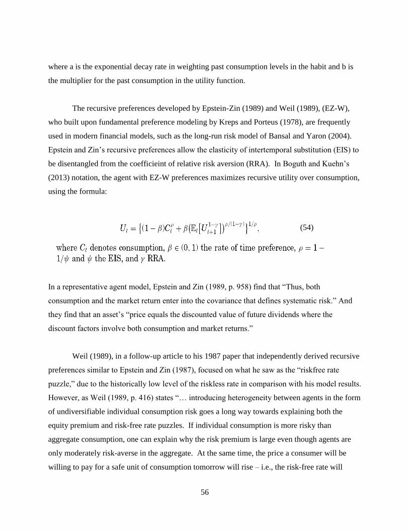
56

where a is the exponential decay rate in weighting past consumption levels in the habit and b is

the multiplier for the past consumption in the utility function.

The recursive preferences developed by Epstein-Zin (1989) and Weil (1989), (EZ-W),

who built upon fundamental preference modeling by Kreps and Porteus (1978), are frequently

used in modern financial models, such as the long-run risk model of Bansal and Yaron (2004).

Epstein and Zin’s recursive preferences allow the elasticity of intertemporal substitution (EIS) to

be disentangled from the coefficieint of relative risk aversion (RRA). In Boguth and Kuehn’s

(2013) notation, the agent with EZ-W preferences maximizes recursive utility over consumption,

using the formula:

In a representative agent model, Epstein and Zin (1989, p. 958) find that “Thus, both

consumption and the market return enter into the covariance that defines systematic risk.” And

they find that an asset’s “price equals the discounted value of future dividends where the

discount factors involve both consumption and market returns.”

Weil (1989), in a follow-up article to his 1987 paper that independently derived recursive

preferences similar to Epstein and Zin (1987), focused on what he saw as the “riskfree rate

puzzle,” due to the historically low level of the riskless rate in comparison with his model results.

However, as Weil (1989, p. 416) states “… introducing heterogeneity between agents in the form

of undiversifiable individual consumption risk goes a long way towards explaining both the

equity premium and risk-free rate puzzles. If individual consumption is more risky than

aggregate consumption, one can explain why the risk premium is large even though agents are

only moderately risk-averse in the aggregate. At the same time, the price a consumer will be

willing to pay for a safe unit of consumption tomorrow will rise – i.e., the risk-free rate will

(54)

57

decrease. Therefore, the existence of heterogeneity and of market imperfections is likely to hold

center stage in the explanation of the equity premium and risk-free rate puzzles.” This leads

nicely into our next section on limited participation, incomplete markets and much larger

individual consumption risks than aggregate per capita consumption risks.

VII. Limited Participation and Incomplete Markets

Mankiw and Zeldes (1991) were first to consider the implications of limited

participation in asset markets. Their article, using the Panel Study of Income Dynamics (PSID),

separates and analyzes the consumption of stockholder and non-stockholder households to

explain the equity risk premium, given that stockholders only accounted for 25% of the whole

US households in 1984. The authors argue that: “One group is involved in the stock market and

is at an interior solution with respect to the holding of stocks, and the other group holds no stocks

at all. The relationship between aggregate consumption and the stock market considered above

is no longer valid, because aggregate consumption includes the consumption of both the

individuals who satisfy the first-order conditions and those who do not.”

Mankiw and Zeldes’s find that stockholder consumption growth has higher volatility and

correlation with the market risk premium than non-stockholder consumption growth. As Table

17 shows, stockholders have a correlation of consumption growth with stock returns equal to

0.49, almost 5 times as large as non-stockholders, who have a correlation of 0.10. Volatility of

stockholders’ consumption growth is 0.032, almost 60% higher than for non-stockholders at

0.020. The combination of higher correlation and higher volatility gives stockholders a

covariance of consumption with stock market returns that is 7 times higher. Mankiw and Zeldes

then compute that the implied constant relative risk aversion for a “representative shareholder”

that is consistent with these statistics drops to about a third the level implied by full participation,

from 100 to 35.

58

Table 17

Source: Mankiw and Zeldes (1991).

The estimate of 35 for the constant relative risk aversion of a representative shareholder

is still implausibly large, and might be caused by the extremely small sample (1970-1984 annual

data) of only 14 annual food consumption growth observations and the assumption that

stockholding status remains unchanged for each household throughout the whole sample period,

as well as the assumption of constant relative risk aversion. Therefore, the size of equity risk

premium is reduced per their results, though it is still not fully resolved due to data limitations

and/or misspecification of the form of the representative shareholder’s utility function. Although

the short sample period is a major limitation, the observed differences in estimtaes consumption

correlation, volatility, covariance and the implied risk aversion parameters of these two groups

shown are dramatic enough to stimulate future research.

Heaton and Lucas (1992, 1996) have two important articles on incomplete markets and

the volatilities of individuals’ consumption growths vis-a-vis aggregate consumption growth. In

the 1992 paper, Heaton and Lucas cleverly employ a 3-period, 2-person model to demonstrate

how market incompleteness, combined with market frictions (such as borrowing and short-sale

constraints, as well as transactions costs), can explain the equity risk premium. The market is

incomplete in having uninsurable labor income shocks, either transitory or permanent. By setting

59

up 3 periods in the model, they are able to model trade, as well as to differentiate between

transitory and permanent shocks to income. And with 2 heterogeneous agents in the model, they

are able to model unemployment risk in a possible recession. They find that the assumed market

structure has a large and systematic impact on predicted asset prices. They also note that whether

consumers use asset markets to smooth consumption depends critically on the persistence of the

idiosyncratic shocks. They point out that “The ability to self-insure diminishes as shocks become

more persistent, because more persistent shocks have a larger impact on permanent income and

hence on desired consumption.” This Heaton-Lucas (1992) model is very thought-provoking,

but perhaps a problem is that there is so much model flexibility that it seems possible to explain

almost any empirical data.

In their 1996 article, Heaton and Lucas decompose the two effects of transactions costs

on the equity premium. The direct effect is because individuals equate marginal benefits, net of

transactions costs. The indirect effect occurs because transactions costs result in individual

consumption that more closely tracks individual income. In the simulations, they find that the

direct effect dominates and can produce a sizable equity premium only if transactions costs are

large or the quantity of tradable assets is limited. They cannot resolve whether or not there is a

realistic assumption about transactions costs that can simultaneously explain the low volatility of

short bond rates and the high volatility of stock returns. They do seem to recognize that taxation

of capital gains based on realizations is a form of a very large transaction costs on assets with

high appreciation that could lead to concentrated portfolios in their model.

Two insightful articles documenting inefficient allocations of consumption and analyzing

their implications were published in the August 2002 issue of the Journal of Political Economy

by Brav, Constantinides and Geczy (BCG), and by Vissing-Jorgensen (V-J), respectively. In

both articles, the authors use the data set provided by the U.S. Bureau of Labor Statistics in its

Consumer Expenditure Survey. BCG provide an excellent detailed explanation of this quarterly

series of cross-sections of household level consumption data. Each quarter approximately 5,000

households are surveyed about their spending on a list of consumption goods and services that

account for approximately 95% of all household expenditures. Households are chosen randomly

according to stratification criteria determined by the U.S. Census and are surveyed for 5 quarters

60

in a row, one training quarter and four regular ones. Every quarter 1/5 of the sample is replaced

by a newly selected household, so 4/5 of the sample is the same from one quarter to the next.

The data started in 1980 Q1; however, they omit the first two years since Attanasio and Weber

(1995) explained that the 1980 and 1981 data are of questionable quality. The following table

from BCG’s article gives the summary statistics for per capita consumption of households that

are sampled quarterly starting in January, February and March tranches, respectively:

Table 18

NOTE—We present summary statistics on the quarterly per capita consumption of nondurables and services by

households for the period 1982:1-1996:1. The household’s consumption of nondurables and services is calculated

by aggregating the household’s quarterly consumption across the consumption categories that constitute the

definition of nondurables and services. We employ aggregation weights that adhere to the NIPA definitions of

consumption of nondurables and services. The household consumption data are filtered using the methods

described in Sec. III C and are deflated to the 1996:1 level, using the CPI for consumption of nondurables and

services. We obtain the CPI series from the BLS through Citibase. We report sample means and standard

deviations for both the level of consumption and consumption growth for a variety of definitions of asset holders

as well as summary statistics on the number of observations in the particular asset-holding layer. Asset holders

are defined as the households in the database that report total assets, in 1996-adjusted dollars. We present

summary statistics separately for each of the three tranches (interview groups) labeled January, February, and

March.

Source: Brav, Constantinides, Geczy (2002).

61

The estimated standard deviation of real consumption growth for these subsets of

households, which are given in the far right hand column of the above table is particularly

informative. Quarterly growth rates have volatilities from 6% to 12%, with wealthier households

having higher volatilities. If consumption growth was independent from quarter to quarter, these

would annualize proportionally to the square root of time, so the annualized volatilities of real

consumption growth would range from 12% to 24%, which is quite a lot of volatility and is

considerable above the approximately 1.0% annualized volatility of aggregate per capita

consumption in the postwar period in the U.S. and 3.6% from 1889-1978, as given in Mehra and

Prescott’s Table 2. This level of volatility in actual individual household level consumption and

limited participation households is one potential rationale for the equity premium puzzle.

Brav, Constantinides and Geczy have a dual goal of investigating the pricing implications

of the incompleteness of markets that insure against idiosyncratic income shocks and the limited

participation of households in the capital markets. BCG define a “stochastic discount factor”

(SDF) or “pricing kernel,” mt, as a function that has the property that for all assets j:

(55)

And applying this to any two assets, such as the market portfolio M and riskfree rate F we have:

(56)

They note that, quite generally, due to the Euler equations of 6’ and 6’’, every individual’s

marginal rate of substitution of consumption (uts’/u0’) across dates and states should be a valid

SDF. And they point out that any weighted sum of the households’ SDFs is also a valid SDF.

This is true whether markets are complete or incomplete. Given this, they compute the

“unexplained mean premium” statistic, u, from historic data for the equity risk premium as

follows:

(57)

They also examine the “value premium” by using returns for high book/market and low

book/market portfolios and computing a “conditional Euler equation, where the attribute of

book/market is the conditioning variable.” Their unexplained-premium statistic for this is:

62

(58)

Then, using an assumption of power utility/constant relative risk aversion, BCG estimate

the individual household’s marginal rate of substitution by raising the household’s consumption

growth to a power equal to the negative of the RRA coefficient. With a time discount factor of

β=e-ρt

and α=RRA in BCG’s notation, the SDF for a group of households is:

(59)

BCG filter the data so that a few extreme outliers do not dominate the results and then test the

null hypothesis that the Euler equations hold and the mean values of the unexplained premium

statistics are individually zero.

Some of Brav, Constantinides and Geczy’s (2002) test results are as follows: using

constant relative risk aversion values from 0 to 9, they find that the unexplained equity risk

premium test statistic is positive for low values of CRRA and negative for high CRRA, crossing

zero at CRRA between 3 and 4, a range that is viewed as plausible by many economists. When

skewness in consumption growth is considered, the unexplained equity premium remains

positive for all levels of CRRA from 0 to 9 and even increases as CRRA increases, but the

amount is statistically insignificant for CRRA greater than 2. Without considering skewness in

consumption growth, the unexplained premium of value stocks over growth stocks crosses zero

when CRRA is between 3 and 4, and crosses with CRRA between 4 and 5 when skewness is

considered. Thus, for very reasonable levels of a “representative household’s” constant relative

risk aversion, BCG appear to provide an explanation for a higher risk premium for the value

stock portfolio compared to the growth stock portfolio based on limited participation of

households in incomplete capital markets.

Vissing-Jorgensen (V-J, 2002) focused on estimating the “elasticity of intertemporal

substitution” (EIS) with the CES data, using information on asset holdings to identify limited

participation in stock and bond markets. As V-J states, “The elasticity of intertemporal

substitution determines how much consumers change change their expected consumption growth

63

rate in response to changes in the expected return to any such asset.” Using the riskless rate, it

would be the change in expected consumption growth for a 1% change in the interest rate. As

the riskless interest rate increases, consumers reduce current consumption and have more to

consume in the future, so the expected growth rate of consumption increases. The amount of that

sensitivity is the EIS. A high EIS means that consumers are willing to vary their growth rate

quite a lot in response to interest rate moves, giving a higher volatility of the lifetime

consumption path. This would be consistent with a higher tolerance for lifetime consumption

risk and a lower degree of risk aversion. Thus, as we saw in the term structure theory equation

30, in the CRRA-lognormal model, the EIS would equal the inverse of relative risk aversion, i.e.,

EIS = 1/RRA. However, as pointed out by Hall (1988) and others since then, EIS can certainly

be quite different from relative risk tolerance (the inverse of RRA) when preferences have time

complementarity. More precisely, risk aversion is perhaps best thought of with regard to

intratemporal (timeless) gambles or choices among different risky assets at a point in time,

whereas the EIS is more a descriptor of intertemporal responses to changes in the reward for

deferring consumption.

Vissing-Jorgensen uses the micro data from the U.S. Consumer Expenditure Survey to

argue that accounting for limited asset market participation is crucial for obtaining consistent

estimates of the EIS. As she says, “The Euler equation should hold for a given household only if

the household holds a nonzero position in the asset.” If households do not hold an asset, there is

little or no reason why they would vary their consumption in response to changes in its expected

return. Including them in estimates of EIS could lead to substantially downward biased

estimates. Using data for stockholders, V-J estimates EIS to be approximately 0.3 to 0.4,

whereas for bondholders the EIS estimates are approximately 0.8 to 1.0. Inverting these

numbers gives a CRRA estimate of 2.5 to 3.3 using the stockholder data, and gives an estimate

of 1.0 to 1.25 using the bondholder data.

To estimate the EIS, Vissing-Jorgensen estimated the following equation:

64

Vissing-Jorgensen does the estimation using GMM with three different sets of

instrumental variables: (1) has the log dividend/price ratio, (2) has that and lagged real stock

return, and (3) has the dividend/price ratio, the bond horizon premium and the bond default

premium. Her results are in Table 19. They show that the EIS for stockholders is approximately

0.30, which is much larger than the 0.06 for nonstockholders, a value that shows little sensitivity

of nonstockholders to returns in the stock market. Thus, stockholders show much more

willingness to respond to better returns than do nonstockholders. Further rows of the table show

that this is even more true for the wealthier households, as the lowest 1/3 households by wealth

have an estimated EIS of 0.05, the middle 1/3 have an EIS of 0.18 and the wealthiest 1/3 have an

EIS of 0.49. Thus, Vissing-Jorgensen showed that limited asset market participation is very

important for estimating the elasticity of intertemporal substitution, EIS. Differences across

stockholders and nonstockholders, as well as between bondholders and nonbondholders, are

large and statistically significant. This research should be quite useful to the Federal Reserve

and other policy makers as they estimate the likely responses of consumers to changes in interest

rates and risky investment returns.

(60)

65

Table 19

Source: Vissing-Jorgensen (2002).

Using updated household level CES data (with help from Dana Kiku, of the University of

Illinois), we computed the volatility of real consumption growth for households of sizes 1, then

for 2-3, and 4+ members, as well as by 3 levels of income – Upper 1/3, Middle 1/3 and Lower

1/3. Individual percentage consumption growth volatility in Table 20 below compares with

Wald

Test

Equals σ

Wald

Test

Equals σ

All 0.10 0.37

（0.07） （0.23）

Stockholders 0.30 0.93

（0.15） （0.37）

Nonstockholders 0.06 0.11

（0.08） （0.27）

Bottom layer 0.05 0.99

（0.19） （0.66）

Middle layer 0.18 0.29

（0.27） （0.55）

Top layer 0.49 1.65

（0.33） （0.52）

Nonstockholders vs. stockholders 3.26 4.03

（0.07） （0.05）

Nonstockholders vs. top layer 2.15 8.06

（0.14） 0.01

All 0.20 0.68

（0.17） （0.46）

Stockholders 0.70 2.62

（0.5） （0.89）

Nonstockholders 0.08 0.05

（0.14） （0.48）

Nonstockholders vs. stockholders 1.73 8.37

（0.19） （0.004）

1. All Household Sizes

2. Single-Individual Households

B. Euler Equation for Treasury Bills

1. All Household Sizes

2. Single-Individual Households

Instrument Set 1:

A. Euler Equation for Stocks

GMM Estimation of Log-Linearized Euler Equations: Real Treasury Bill Return and Real Value-

Weighted NYSE Return, Separate Estimations (CEX,1982-96,Semiannual Data)

66

volatility of just approximately 1.0% for aggregate per capita consumption growth of

nondurables and services. The calculations that individuals actually experience real consumption

volatility more than 7% should reduce constant relative risk aversion estimates by a factor of at

least 7, which would bring many risk aversion estimates into the 1 to 10 range that many

economists believe is reasonable.

Table 20

Constantinides and Duffie (1996) developed an elegant theoretical model of the impact of

substantial heterogeneity of individuals’ incomes on asset pricing. They model consumers who

have power utility functions (CRRA), but have uninsurable, persistent and heteroscedastic labor

income shocks. This is quite a reasonable and important model, given the differences we have

seen in the preceding tables for households’ consumption volatility versus aggregate

consumption volatility. Constantinides and Duffie observe (p. 223) “… the model predicts that a

potential source of the equity premium is the covariance of the securities returns with the cross-

sectional variance of individual consumers’ consumption growth, a source that is (under typical

conditions) irrelevant in an economy with full consumption insurance.” With CRRA=α and their

carefully built model of individual income shocks, the Euler equation is derived in terms of

aggregate consumption, Ct+1, and a measure, 𝑦𝑡+12 , which “…is interpreted as the variance of the

cross-sectional distribution of log [(𝐶𝑖,𝑡+1/𝐶𝑡+1)/(𝐶𝑖,𝑡/𝐶𝑡)]” where i=1 to N represents different

individuals (p. 229):

(61)

Lower

1/3 

Middle

1/3 

Upper

1/3 

Row

Average

1 person 11.7 12.4 12.5 9.4

2-3 person 9.8 8.4 9.1 6.2

4 person 13.5 10.3 7.6 6.7

Column Average 8.6 8 7.3 6.4

Family

Size

Income

NDS Consumption Growth Volatility

67

If consumers were identical in preferences and incomes, then y2 would be zero and the Euler

equation reduces to the familiar one for CRRA.

Constantinides and Duffie also prove the equilibrium solution of their heterogeneous

consumer model is isomorphic to that of the representative consumer model, by assuming

specific forms of the 𝑦𝑡 function, such as the following:

(62)

Substituting this function into the general Euler equation gives a reduced form Euler

equation corresponding to the classical one with representative consumers:

(63)

where the modified risk aversion coefficient ��, deviates from the one without heterogeneity, α.

(64)

Though this specific function of 𝑦𝑡 is rejected when they test the Euler equation with data, their

discussion is of general interest in explaining the size of the equity risk premium. If the cross-

sectional variation is countercyclical, b is negative and the modified risk aversion �� is higher

than the classical risk aversion parameter α . Therefore, an econometrician unaware of the

heterogeneity would mistake �� as α , and overestimate the risk aversion parameter under a

homogenous model.

The Constantinides-Duffie derivation of the importance for asset pricing of the cross-

sectional heterogeneity of individual consumers’ actual incomes and consumption volatilities,

rather than just the volatility of the aggregate, is a significant and economically intuitive result in

asset pricing. It seems that almost nobody has consumption volatility as low as the aggregate

measures, so is it not intuitive that market pricing would reflect covariances with individuals’

actual marginal utilities, which reflect their individual consumption volatilities? This is an area

worthy of additional research. We need to understand the consistency of this result with

68

Breeden’s (1979) continuous-time CCAPM with heterogeneous consumers, wherein consumer

spending can be aggregated in asset pricing results.

VIII. 1990s Models of Changing Conditional Risks: Risk Factors and Risk Premia

The perceived failure of consumption-based asset pricing models in explaining the equity

premium and the cross-section of returns (e.g., see Mehra-Prescott (1985) and Breeden, Gibbons,

Litzenberger (1989)), motivated over the subsequent decade both theoretical research on more

general preferences with time complementarity and habits, and empirical research on multiple

factors, conditional risks and changing risk premiums through time. As shown by Sundaresan

(1989) and Epstein-Zin (1989), preferences with time complementarity justified multiple factors ,

(with market betas as well as consumption betas), and testing proceeded seeking multiple factors

and multiple prices of risk, along the lines of Merton’s Intertemporal CAPM and Ross’s

Arbitrage Pricing Theory (APT).

Several articles were produced that appeared to demonstrate predictability in mean

returns, a result that researchers had doubted based on earlier research on market efficiency.

However, researchers began to realize that if risks change through time and in different

economic conditions (e.g., in risky recessions vs. stable growth periods), then it is economically

sensible that mean returns should also vary with economic conditions to reward investors more

when risk is higher. Keim and Stambaugh (1986) found that the credit yield spread of Baa rated

bonds over Aaa rated bonds had some ability to predict future bond and stock returns. Fama and

French (1988) and Campbell and Shiller (1988) found that trailing dividend yield, an easily

measured variable, had ability to predict returns, especially over the longer term, as much as 7

years out. Kandel and Stambaugh (1989) used dividend yield, a credit risk yield spread and the

slope of the term structure to model time-varying risk premiums. In a particularly insightful

article, Ferson and Harvey (1991) built on this prior work to model both changing conditional

betas and changing conditional risk premiums, finding that the changing risk premium for beta

was a much larger explanatory variable in returns than are changing betas for 12 major industries,

10 deciles of size-ranked portfolios, and government and corporate bonds and Treasury bills.

The right hand side of the following table from Ferson-Harvey shows these results:

69

Table 21

NOTE—All rates of return are in excess of the 1-month Treasury bill rate. Decile 1 represents the excess returns on

the decile of the smallest-valued firms on the NYSE. Decile 10 represents the excess returns on the largest decile

of NYSE stocks. The figures are the percentages of the sample variances of predicted excess returns, using a

multibeta asset pricing model, which are allocated to different sources of predictable variation.

Source: Ferson and Harvey (1991, Table 8)

Ferson and Harvey show that the estimated risk premium for equities varies with

economic conditions, generally increasing in recessions (as risk and premiums per unit of risk

increase ) and decreasing during growth periods, when risk and premiums per unit of risk appear

to subside. The following graph shows this result:

70

Figure 10

FIG.1.—Fitted values from a regression of the price of market beta on the instrumental variables. The values for

the price of market beta are the estimated coefficients from a cross-sectional regression each month of 25

portfolio returns on estimates of the market beta coefficients. The monthly estimates of the price of beta are

regressed over time on the predetermined variables summarized in table 3. The regressions include dummy

variables that allow each of the slope coefficients to differ in January from their values in the other months. The

fitted values of the regression are shown in this graph. The dashed line represents the January observations; the

solid line represents the other 11 months.

Source: Ferson and Harvey (1991), Figure 1.

In 1992 and 1993, Fama and French, in now classic articles, showed that average returns

on stocks and bonds were related to five major explanatory factors (3 from stocks, 2 from bonds):

(1) a general stock market factor risk estimated by market betas, (2) a factor related to

differential performance of small stocks versus large stocks (SMB for small minus big), (3) a

factor related to differential performance of high versus low book/market stocks, which picks up

a premium of value versus growth stocks (HML for high minus low), (4) a term premium

variable measured by the return on long-term government bonds, less that on 1-month Treasury

bills, and (5) a default premium, measured by the return on corporate bonds, less that of

government bonds. As the following regression from Fama and French (1993, eq. 1) shows, the

market portfolio’s excess return is a “hodgepodge” of the common risk factors, even showing

statistically significant common variation with the two bond market related factors (t-statistics in

parentheses, R2 = 0.38):

71

𝑅𝑀 − 𝑅𝐹 = 0.50 + 0.44𝑆𝑀𝐵 − 0.63𝐻𝑀𝐿 + 0.81𝑇𝐸𝑅𝑀 + 0.79𝐷𝐸𝐹 + 𝑒 (2.55) (6.48) (−8.23) (9.09) (4.62)

(65)

This regression shows that the stock market portfolio tends to do better when small stocks

outperform large stocks, when growth stocks beat value stocks, when long-term government

bonds beat T-bills, and when credit risk is rewarded.

Fama and French’s papers raised two new puzzles that stimulated a large literature in

subsequent years. In their 1992 classic, they found that the “relation between market beta and

average return is flat.” Contrary to the prediction of the CAPM, they found no significant reward

for taking equity beta risk in their 1963-1991 sample. The first puzzle they is that small stocks

outperformed large stocks (SMB effect >0 on average), even after taking into account equity

market beta differentials. The second puzzle is that value stocks outperformed growth stocks

(HML effect >0 on average), also after taking into account equity market beta differentials.

Table 22

Table 23

Source: Fama and French (1992).

72

Fama and French’s surprising results have been partially attributed to the relatively small

sample (1963-1991) and it has been noted that their estimates have high standard errors. While

the average returns versus betas relationship improves with longer data series and more asset

classes, the size and book/market results have been demonstrated over longer time periods. As

we shall see in key articles by Lettau and Ludvigson (2001b) and Jagannathan and Wang (2007)

on consumption-based asset pricing, perhaps the size and value/growth effects can be explained

by their differential conditional consumption risks. For example, value stocks are shown to have

relatively higher consumption betas in recessions, when risks and risk premiums per unit of risk

are high, and lower conditional consumption betas in growth periods, when risks and risk

premiums per unit of risk are low. This effect makes the unconditional risk premium for value

stocks larger, due to the positive correlation of their consumption betas with market risk

premiums. Alternatively viewed, the growth stock portfolio has an unconditional convex relation

to consumption growth indicated by a higher CCAPM beta conditional on expansion periods and

a lower CCAPM beta conditional on recessionary periods. Conversely, the value stock portfolio

has an unconditional concave relation to consumption indicated by a lower CCAPM beta

conditional on expansion periods and higher CCAPM beta conditional on recessionary periods.

Consistent with Jagannathan and Wangs findings, the analysis of Kraus and Litzenberger (1983)

suggests that under decreasing absolute risk aversion individual would have a preference for

positive skewness and the unconditional risk premium for the growth stock portfolio would cet.

par. be less than that for the value stock portfolio.

Jagannathan and Wang (1996) significantly advanced the case for modeling conditional

variation in betas and risk premiums. They modeled changes in betas as being related to the

credit yield spread between low and high grade bonds, which is sensitive to perceived risks of

default and is quite related to the state of the economy, as was shown earlier in Figure __ relating

credit spreads to the unemployment rate. Additionally, they use a proxy for human capital to get

a better estimate of returns on the true, but unobservable market portfolio. With the broader

market portfolio, combined with changing conditional risks and conditional risk premiums, they

are able to explain much of the size effect identified by Fama and French.

73

In the next section, we will examine habit formation models, which provided strong

empirical support for consumption-based asset pricing. Subsequent sections will show how this

evidence was then enhanced by works on conditional consumption betas (Lettau-Ludvigson

(2001b) and Jagannathan-Wang (2007)), ultimate consumption betas (Parker-Julliard (2005)),

and the long-run risk model of Bansal and Yaron (2004, and follow up articles).

IX. Habit Formation Models: Campbell-Cochrane (1999)

In a major “second generation” consumption-based asset pricing model, 20+ years after

the original CCAPM, Campbell and Cochrane (1999) developed a landmark model of asset

pricing using a utility function of a representative individual with an external habit. Under an

external habit individual do not consider the impact of their current consumption decision on

their habit in future periods, which simplifies the optimization problem. Campbell and Cochrane

successfully employ the utility function to fit a countercyclical equity risk premium. Three

features of their model are worthy of note: (1) a slow-moving external habit based on per capital

consumption, (2) i.i.d. per capita consumption growth and (3) highly nonlinear utility and

relative risk aversion that approaches infinity near the external habit level. By assuming a

representative individual with an external habit, they sidestep the aggregation of heterogeneous

individuals, limited participation issues, and the impact of current consumption decisions on the

current or future habit. Their model is able to generate counter-cyclical fluctuations and long-

term predictability of equity risk premium by having relative risk aversion become arbitrarily

large as current consumption approaches the external habit.

Individuals are assumed to maximize:

E∑ 𝛿𝑡∞𝑡=0

(𝐶𝑡−𝑋𝑡)1−𝛾−1

1−𝛾 (66)

Note that this preference function is similar to an extended power utility function with an

intercept equal to minus the external habit. This utility function displays decreasing relative risk

aversion, and relative risk aversion approaches infinity as the representative individual’s

consumption declines toward the external habit. Thus, the habit intuitively seems more like a

subsistence level of consumption, rather than a habit motivated by consumption envy that the

74

“keep up with the Joneses” motive seems to suggest. Since the individual views the habit as

exogenous, the representative individual’s consumption decision does not consider the impact on

the habit. Under the assumption of identical powers, γ, this preference function could be

aggregated from individual extended power utility with diverse external habit levels. The

modeling of the aggregated external habit as a lagged function of past per capita consumption is

intuitive. The preference function is not defined for a negative habit level, which requires

consumption to be strictly above the habit. The above preference function could be used with a

stochastic process on per capita consumption that was consistent with this constraint. For

example, if Ct followed a shifted lognormal process with a shift parameter of Xt, realizations of

excess consumption would be positive without making Xt a function of Ct, which would not be

intuitive for a subsistence level of consumption. However, Campbell and Cochrane assume that

per capita consumption is lognormally distributed and make the external habit an implicit

function of current consumption, such that the external habit’s downward moves assure that

excess consumption is positive for all realizations of per capita consumption.

Campbell and Cochrane use a variable called the “surplus consumption ratio” as the

difference between per capita consumption in the economy and the representative individual’s

external habit level, Xt, expressed as a fraction of per capita consumption:

𝑆𝑡𝑎 =

𝐶𝑡𝑎−X𝑡

𝐶𝑡𝑎 (67)

The log surplus consumption function sta is modelled as an AR(1) process with a speed

depending on parameter ϕ and a monotonically decreasing sensitivity function λ(sta), where

lower case letters are logs of the upper case variables:

(68)

Substituting the surplus consumption ratio into the AR(1) process demonstrates that the

external habit, Xt, adjusts to Ct, as well as to the history of average per capita consumption. The

external habit adjusts slowly and geometrically to past consumption with coefficient 𝜙. The log

transformation constrains the surplus consumption to be non-negative. They impose several

restrictions on the parameters to produce a constant risk-free rate and a predetermined habit level

75

around the steady state, so as to make sure the excess co-moves with consumption, but is always

positive. Under their specification as Ct approaches zero, changes in Xt offset the impact of

changes in Ct on the excess consumption ratio. The justification for this specification for a

learned habit, which intuitively should be slowly moving in response to past levels of

consumption of others, is not provided. The implications of their parameter specifications are

shown in the graphs below.

Figure 11 Figure 12

They then price bonds and stocks using classic Euler equations and choose the free

parameters in the model to fit the moments of post-war data. Empirical calibration shows their

model can fulfill its goals and generate a non-linear countercyclical risk premium and cyclical

equity volatility. When surplus consumption drops to near zero during recessions, both the equity

risk premium and volatility of stock returns increase at an increasing pace, as shown in the

following figures from their article:

Figure 13 Figure 14

76

Also, as Table 24 from Campbell and Cochrane shows, there are enough parameters that

their simulated data can fit the four moments of the post-war data quite well, fitting the equity

risk premium and its Sharpe ratio almost perfectly, as well as consumption growth’s mean and

volatility and equity market volatility:

Table 24

Source: Campbell and Cochrane (1999)

As one of the early papers modeling the effects of habit formation utility functions on

asset pricing, Campbell and Cochrane (1999) plays an important role in modeling the time-

varying and countercyclical risk premium by a having a slowly adjusting habit level and highly

nonlinear utility responses. Effectively, by making relative risk aversion become very large as

excess consumption approaches zero, large variations in risk premiums can be explained. C-C

observe (p. 244): “Risk aversion is about 80 at the steady state … rises to values in the hundreds

for low surplus consumption ratios and is still as high as 60 at the maximum surplus

consumption ratio.” Their empirical results do not seem to depend upon time complementarity

per se. In retrospect, this helps us see that the whole literature on excess volatility seems to have

implicitly focused on constant relative risk aversion. Of course, a potential drawback is that

having many parameters and imposing some delicate restrictions gives considerable flexibility to

overfit the data. Out of sample testing using the in sample parameter would be informative.

77

Campbell and Cochrane (1999) have a very important and plausible prediction that

relative risk aversion and risk premiums increase quite nonlinearly as surplus consumption goes

towards zero, as in major recessions. To amplify on this important aspect of changes in risk

premiums, we have examined data for real consumption growth and the level and changes in the

unemployment rate over long time horizons. We started with Shiller’s (2014) long-term

database for stock prices and consumption growth, and added to this long-term data on the

unemployment rate from NBER and the St. Louis Federal Reserve historical database, FRED.

The NBER has a monthly series of unemployment rates that goes back to April, 1929, and we

used monthly data on employment changes from the 1932 Supplement to the Survey of Current

Business to estimate monthly unemployment rates from January of 1923 to April 1929. Given

this, our first data point for the 12-month change in the unemployment rate is for January 1924,

so we have just over 90 years of monthly data to July 2014.

We invert Shiller’s long-term estimates of his “Cyclically Adjusted Price Earnings” Ratio

(CAPE) to get an earnings yield number (biased low), from which we subtract the long-term (10-

year) U.S. Treasury interest rate to get a long data series of estimated “risk premiums” for U.S.

equities, E/P – Rf . These are surely biased low, as earnings grow over time, so forward forecasts

will be higher than these backward looking earnings numbers. To test the stochastic properties

of this backward looking earnings yield with a forward one, we obtained monthly observations

of the 12-month forward S&P 500 earnings estimates from 1986 to August 2014 from Ed

Yardeni’s website and computed a forward looking earnings yield based on that series. The

following graph shows that the Shiller-type backward looking, long-term earnings yield gap is

highly correlated (ρ= 0.95) from 1986 to 2014 with the forward looking earnings yields: As

expected earnings yields based on next 12 months earnings estimates are persistently higher than

the 10-year historic earnings divided by current price. The bias averages about 3% over the long

term. Furthermore, corporate investment at rates of return in excess of capital cost would result

in the forward looking earnings yield being a downward biased estimate of the expected rate of

return. However, this bias should be greater in prosperous period with higher returns on real

investment than in recessionary period with lower returns on real investment.

78

Figure 15

Given this high correlation of 10-year historical and 1-year forward “yield gaps”, we feel it is

not unreasonable to look at a Shiller-type earnings yield gap time series as an estimate of what

the stochastic properties of the time series of investors’ forward earnings yield spreads to riskfree

rates were in past years. Given the cyclical bias of forward earnings yields as estimates of

expected returns, higher earnings yield spreads in recessionary periods is consistent with higher

risk premiums in recessionary periods.

Our next figure shows the relationship of the 12-month changes in the estimated equity

risk premium to 12-month changes in the unemployment rate. As the graphs shows, the series

are highly correlated. When the economy falls into recession and the unemployment rate jumps,

the estimated risk premium also tends to jump. We find a very strong and nonlinear relationship

of the estimated risk premium to the unemployment rate and to real consumption growth. This

helps us to understand why the Campbell-Cochrane (1999) model is very helpful in modeling

movements in the real economy. The correlation of the moves in estimated risk premium and

changes in the unemployment rate is 0.40 over the entire 1924-2014 sample, and is 0.53 if the

World War II years of 1939-1947 are excluded, as unemployment fell sharply in WWII, while

risk and risk premia increased, an abnormal economy.

79

Figure 16

Figure 17, shows that changes in the unemployment rate explain changes (R2 = 0.27) in the

estimated risk premium, a statistically significant relation (with a Newey-West t-statistic of 4.3.)

Figure 17

80

The next figure shows that the picture is much the same if one uses real growth of

consumption of nondurables and services in modeling changes in the equity risk premium.

When real consumption growth is high and the economy is good, Campbell-Cochrane’s surplus

consumption increases and risk aversion likely drops, along with risk premiums. Note that as

monthly consumption data begins in January 1959, our first data point of 12-month consumption

growth is for January 1960.

Figure 18

The next two graphs show that the picture is very similar if we look at forecasted forward

earnings yields, less the 10-year Treasury yield and compare that yield gap’s moves to moves in

real consumption growth and to changes in the unemployment rate. Once again, the

relationships are all strong and in the right direction. Thus, we believe that, as predicted by

Campbell and Cochrane model, it is quite plausible that relative risk aversion and risk premiums

are indeed significantly countercyclical.

81

Figure 19

Figure 20

In conclusion on this segment, we believe that the external habit formation model and the

forecasted large cyclical swings in relative risk aversion and risk premiums have much to offer to

finance researchers and practitioners that is quite important economically and statistically.

82

X. Resurrecting the CCAPM: Conditional Consumption Risks, Ultimate Risk:

Lettau-Ludvigson (2001), Parker-Julliard (2005) and Jagannathan-Wang (2007)

In a pair of innovative, impactful articles, Lettau and Ludvigson (2001a,b) built an

econometric model where consumption, wealth and labor income are cointegrated, and

consumption’s deviations from the shared trend summarize agents’ expectations of future returns

on the market portfolio. This ties in very nicely with the continuous-time intertemporal portfolio

theory of Merton (1971, 1973) and Breeden (1979, 1984). It also is consistent with prior

analyses of consumption responses to shocks to permanent and transitory income. In Breeden’s

(1984) theoretical analysis (Section II, eq. 15 in this article), optimal consumption’s sensitivities

to the state variables that describe the investment and income opportunity set are proportional

and opposite to the compensating variations in wealth for changes in those state variables. If the

opportunity set improves, compensating variations in wealth are negative and we expect most

individuals to respond positively with increased consumer spending. In contrast, if the

opportunity set is believed to deteriorate, individuals optimally reduce consumption spending

today to smooth their forward looking lifetime consumption paths.

Going backwards from consumption’s moves, a high level of consumption relative to

wealth and income indicates a good investment and income opportunity set, whereas a low

consumption/wealth ratio is indicative of views of a poor investment and income opportunity set

(perhaps a poor job market?). Lettau and Ludvigson (2001a) estimate the cointegrating

relationship among consumption, wealth and income, and use positive deviations of consumption

from the shared trend as a predictor of better than normal investment returns and negative

deviations as predictors of poor future returns.6 Using a dynamic least squares technique that

accounts for both leading and lagging relationships among the cointegrated variables, they

generated the following point estimates for the parameters of shared consumption, labor income

and wealth (with small letters indicating natural logarithms of real nondurables and services

6 Do note that it is entirely possible both in theory and in practice that movements in volatility could be offsetting to

the impact of movements in mean returns, and cause the relation to not be as sought by Lettau and Ludvigson. If,

for example, volatility dropped sharply at the same time that mean returns dropped modestly, the Sharpe ratio (slope

of the capital market line) could actually improve, indicating a better investment opportunity set and causing optimal

consumption to increase. Similarly, the mean return on the market could increase modestly at a time that volatility

increased sharply, and optimal consumption would decline. These results were actually found by Breeden (1989) in

an unpublished working paper presented at the French Finance Association, wherein high consumption growth was

shown to be more a reflection of low future investment risk than it was a reflection of high future investment returns.

83

consumption, asset wealth and labor income per capita, respectively), using data from 1952Q4 to

1998Q3:

𝑐𝑛.𝑡 = 0.61 + 0.31𝑎𝑡 + 0.59𝑦𝑡 (7.96) (11.70) (23.92)

(69)

The residual term, which they denote as “cay,” measures the difference between log

consumption and its conditional expectation based of household net worth and labor income.

From Lettau and Ludvigson’s websites, given another 15 years of data, some substantial data

revisions by the government in 2003, and some changes to their structural model, their current

estimated log consumption trend deviation, using data from 1952Q1 to 2013Q3 is of the form:

cayt = ct – 0.87 - 0.12 at - 0.78 yt (70)

The change in coefficients from 1998 to 2013 indicates that, in describing consumption moves,

labor income has become relatively more important than wealth, which is measured as

“Household Net Worth” reported quarterly by the Federal Reserve, and includes real estate and

bond values, as well as stocks.

Lettau and Ludvigson’s (2001a) results during the time period studied (1952-1998) are

quite strong, finding that “… a one-standard-deviation increase in cay leads to a 220 basis points

rise in the expected real return (in the next quarter) on the S&P Index and about the same rise in

the excess return, roughly a nine percent increase at an annual rate.” The Newey West t-statistic,

corrected for generalized autocorrelation, is above 3.0, which is statistically significant. Longer

horizon forecasts are also impressive. As the following excerpt from their Table VI shows, the

cay variable has significant explanatory power at all intervals from 1 quarter to 6 years, with

robust t-statistics of 3.0 or more:

84

Table 25

Source: Lettau and Ludvigson (2001a), Table VI.

During this period, dividend yield (in log terms, log D minus log P) was less statistically

significant as a forecaster of future real stock returns than in prior studies, but still had strong

significance forecasting 6 years out returns. LL’s cay variable had even stronger explanatory

power for future stock returns for both shorter time horizons (1-4 years) and the longer horizon,

6 years. Panel A shows that consumption deviations were not successful in forecasting future

real consumption growth, which is consistent with Hall’s (1978) prior results. Updating the

statistics with data from 1998 to 2013 from the website data of Lettau and Ludvigson, we find

that a 1 standard deviation move in their cay variable is associated with a move that is about 65

bp less per quarter than in the original study, perhaps 155 bp/quarter, giving a still-large

increment of returns of about 6%-6.5% annualized, rather than the original finding of 9.0%.

In the companion article by Lettau and Ludvigson (2001b) entitled “Resurrecting the

(C)CAPM: A Cross-Sectional Test When Risk Premia Are Time-Varying,” they use their new

consumption trend deviation, cayt, as a “scaling” variable for measuring conditional expected

85

returns of assets. Lettau and Ludvigson first illustrate the poor results of using unconditional

beta estimates in cross-sectional fits of mean returns with market-based CAPM betas (figure a)

and with Consumption CAPM betas (fig. c) for the 25 Fama-French portfolios sorted by size

and book/market. They show the much better fit of mean returns from the Fama-French (1992)

3-factor statistical model (fig b), for which the underlying risk factors are unknown. Finally,

using their cay variable for conditioning, they find that their conditional version of the

Consumption CAPM fits nearly as well as the Fama-French, 3 factor statistical model (fig. d):

Figure 21

Conditional Consumption CAPM Fits Nearly As Well As Fama-French 3-Factor Model

FIG.1.—Realized vs. fitted returns: 25 Fama-French portfolios: a, CAPM; b, Fama-French; c, consumption

CAPM; d, consumption CAPM scaled. The figure shows the pricing errors for each of the 25 Fama-French

portfolios for the four models. Each two-digit number represents one portfolio. The first digit refers to book-to-

market quintiles (1 indicating the portfolio with the lowest book-to-market ratio, 5 with the highest). The pricing

errors are generated using the Fama-MacBeth regressions. The scaling variable is 𝑐𝑎𝑦.

Source: Lettau and Ludvigson (2001b), Figure 1.

86

Lettau and Ludvigson (2001b, p. 1241) note that: “Intuitively, conditioning improves the

fit of the CCAPM because some stocks are more highly correlated with consumption growth in

bad times, when risk or risk aversion is high, than they are in good times, when risk or risk

aversion is low. This conditionality on risk premia is missed by unconditional models because

they assume that those risk premia are constant over time.” This logic is consistent with

Campbell and Cochrane (2000), who argued that conditional models will perform far better than

unconditional models based on the presence of an external habit.

To see the changes in conditional consumption betas between “good states” and “bad

states,” Lettau and Ludvigson denote the good states as those where cay was 1 standard deviation

above the unconditional mean, and bad states as those where cay was 1 standard deviation below

that mean. The estimated conditional consumption betas for the 25 Fama-French size and

book/market sorted portfolios are in the following table.

Table 26

Change in Beta

Portfolio All States Good States* Bad States** Bad-Good

S1B1 Growth 6.4 7.3 5.7 -1.6

S1B2 6.3 5.8 6.6 0.8

S1B3 Small 5.1 4.4 5.6 1.1

S1B4 5.5 4.4 6.2 1.8

S1B5 Value 5.8 3.4 7.4 4.0

S2B1 Growth 4.4 7.7 2.1 -5.6

S2B2 3.6 3.6 3.6 0.0

S2B3 3.9 4.1 3.8 -0.4

S2B4 3.5 2.1 4.5 2.4

S2B5 Value 4.8 3.1 6.0 3.0

S3B1 Growth 2.7 7.4 -0.5 -7.8

S3B2 2.8 3.5 2.3 -1.2

S3B3 2.9 2.0 3.5 1.6

S3B4 2.6 2.6 2.6 0.0

S3B5 Value 3.7 2.7 4.4 1.7

S4B1 Growth 2.0 6.2 -0.9 -7.1

S4B2 2.6 4.8 1.2 -3.6

S4B3 1.9 3.0 1.2 -1.8

S4B4 2.5 2.4 2.6 0.2

S4B5 Value 3.8 3.1 4.3 1.2

S5B1 Growth 1.6 6.1 -1.4 -7.5

S5B2 1.2 2.0 0.6 -1.5

S5B3 Large 2.3 4.1 1.2 -2.9

S5B4 1.2 3.4 -0.3 -3.7

S5B5 Value 3.1 3.3 2.9 -0.5

*Good states are states with cay more than 1 standard deviation above the mean

**Bad states are states with cay more than 1 standard deviation above the mean

Source: Lettau and Ludvigson (2001b)

Conditional Betas in the Consumption CAPM

87

Note the differences in the systematic changes in consumption betas between good and

bad states and how they are related to whether the stocks are growth stocks (B1/B2) or value

stocks (B4/B5). Consumption betas of value stocks increase in bad times, which is when risks

are highest, so their equilibrium returns on average need to be higher, as the data has shown they

are. Thus, Lettau and Ludvigson are able to explain the “value effect” with the conditional

changes in consumption betas. In contrast, betas for growth stocks seem to fall in bad times,

giving them lower consumption risk then. As previously discussed this pattern of conditional

consumption beta indicated that the growth stock portfolio has an unconditional convex relation

to consumption growth and conversely, the value stock portfolio has an unconditional concave

relation to consumption growth. Under decreasing absolute risk aversion there is a preference

for positive skewness and the unconditional risk premium for the growth stock portfolio would,

ceteris paribus, be less than that for the value stock portfolio.

The Campbell and Cochrane (1999) model of external habit formation (and conditionally

changing and nonlinear risks and relative risk aversion), and the Lettau and Ludvigson (2001a, b)

articles were important in reestablishing the Consumption CAPM and consumption-based asset

pricing as a leading model of asset pricing. Both demonstrated that we need more advanced

econometric techniques to properly model changing consumption risks and changing risk

aversion and risk premiums through time and economic scenarios.

In an important article, Parker and Julliard (2005) develop a model of “ultimate

consumption risk,” which captures the longer run relationship of consumption with asset returns.

They argue that “… most importantly, the ultimate risk may be a better measure of the true risk

of an asset if consumption is slow to adjust to returns. If consumption responds with a lag to

changes in wealth, then the contemporaneous covariance of consumption and wealth understates

or mismeasures the true risk of a portfolio. Ultimate consumption risk, on the other hand, can

provide the correct measure of risk under several extant explanations of slow consumption

adjustment, such as some models of (a) measurement error in consumption; (b) costs of

adjusting consumption; (c) nonseparability of marginal utility of consumption from factors such

as labor supply or housing stock, which themselves are constrained to adjust slowly; or (d)

constraints on information flow or calculation so that household behavior is ‘near-rational.’”

88

Their main finding is that ultimate consumption risk can largely explain the cross-

sectional pattern of expected portfolio returns. While the covariance of each portfolio and

contemporaneous consumption growth explains little of the variation in expected returns across

portfolios, at a horizon of three years the ultimate risk to consumption explains 44 to 73 percent

of the variation in expected returns across portfolios, depending on the specification. The

performance of ultimate consumption risk rivals that of the Fama and French (1992) three-factor

model and the Lettau and Ludvigson (2001b) three-factor model, two important linear factor

models that have been used to price the expected returns in the Fama-French portfolios.

Parker and Julliard propose ultimate consumption risk to explain the cross-sectional

heterogeneity of the 25 Fama-French portfolios. By ultimate consumption, they mean that

increasing the consumption growth horizon to longer terms can increase cross-sectional

explanatory power of the canonical CCAPM model, and the optimal point is achieved at 3 years

with a 44-73% R-square, depending on the specifications. Parker and Julliard estimates of the

relationship of the cross-section of returns to consumption risk measured over different horizons

are in the following table:

Table 27

Source: Parker and Julliard (2005), Table 1. Standard errors in parentheses, and Hansen-Jagannathan

distance p-values are in brackets.

Risk Aversion Risk Aversion

Horizon S R2

(%) α ϒ Dist Horizon S R2 α ϒ Dist

(Quarters) (1) (2) (3) (4) (Quarters) (1) (2) (3) (4)

0* 4 0.029 19.9 0.37 7 10 0.019 11 0.36

(0.006) (33.3) [0.000] (0.008) (14.3) [0.000]

0 3 0.023 19 0.37 8 20 0.018 15.1 0.34

(0.005) (41.8) [0.000] (0.006) (13.8) [0.000]

1 2 0.023 10.7 0.37 9 30 0.018 17.9 0.31

(0.007) (27.5) [0.000] (0.005) (12.5) [0.000]

2 5 0.02 14.6 0.37 10 33 0.017 18.6 0.31

(0.009) (24.8) [0.000] (0.005) (13.7) [0.000]

3 10 0.018 17.9 0.36 11 44 0.015 25.4 0.28

(0.009) (23.5) [0.000] (0.006) (16.4) [0.000]

4 4 0.021 9.1 0.37 12 32 0.016 25 0.31

(0.008) (17.2) [0.000] (0.005) (16.5) [0.000]

5 7 0.019 11.7 0.36 13 35 0.012 38.5 0.3

(0.008) (16.3) [0.000] (0.006) (14.0) [0.000]

6 9 0.018 12.6 0.36 14 30 0.014 34.6 0.31

(0.008) (15.3) [0.000] (0.005) (24.6) [0.000]

15 24 0.016 39.4 0.33

(0.008) (24.4) [0.000]

GMM with prespecified weighting matrix

89

where γ is the estimate of relative risk aversion and α is a constant term. From the table, it is

seen that R2 grows from near zero for contemporaneous consumption risk to 44 percent when

consumption risk is measured by cumulative real nondurables consumption growth over the next

11 quarters, almost 3 years. Note that while ultimate consumption risk helps explain the cross-

section of returns, the relative risk aversion estimate is quite high at approximately 25.

Parker and Julliard compare the empirical performance of four models: (1) CCAPM with

only contemporaneous consumption risk, (2) the Fama-French 3-factor model, (3) Lettau and

Ludvigson’s conditional test of the CCAPM using their consumption/wealth ratio, cay, as a

conditioning variable, and (4) ultimate consumption risk over 11 quarters. The results are quite

apparent in the graphs below:

Figure 22

Source: Parker and Julliard (2005).

90

What drives the excellent results for Parker-Julliard’s ultimate consumption risk measure

is the fact that the excess returns of the Fama-French portfolios predict future consumption

growth. As they say, “… both the excess return of small firms less large firms and the excess

return of high-value stocks less low-value stocks predict consumption growth. The joint

predicting power of SMB and HML peaks at 3 years.” However, using the GMM estimator, the

ultimate consumption model with 26 moments and only 3 parameters is still rejected by the over-

identification test, so further analysis is required. While their observations concerning longer

term consumption effects are intuitive, the specification based on declining weights over time

would be more intuitive than equal weighting over a fixed horizon. Figure 24, from Liew and

Vassalou (2000), shows the difference in return to factor portfolios in the year prior to above

average versus below average GDP growth. (See Bodie, Kane and Marcus’s Investments (2010,

Fig. 13.1)). Both small minus big and high minus low portfolios are typically higher prior to

improving GDP growth:

Figure 23

Source: Liew and Vassalou (2000).

-15.73

-1.81

14.98

1.7

17.05

-0.99

4.73

14.77

8.49

3.14

28.65

5.71

21.1423.7

29.01

18.09

-4.09

19.97 19.13 19.5

-20

-15

-10

-5

0

5

10

15

20

25

30

35

Australia Canada France Germany Italy Japan Netherlands Switzerland United

Kingdom

United

States

Size and Book/Market Effects Lead Economic Growth.

Do They Reflect Consumption Risk? Does the Multiperiod CCAPM Explain?

HML SMB

91

In 2007, Jagannathan and Wang (J-W) also provided strong empirical support for

consumption based asset pricing. They propose a theory of consumers who use discretion in

periodically reviewing consumption and investment decisions, as opposed to continuously

optimizing their consumption and investment rules. They argue that consumers are more likely to

review their decision making at tax year ends (in the 4th

quarter) and during economic

contractions. They demonstrate that this helps explain the unsatisfactory previous testing results

of the CCAPM. They compute the excess returns and consumption betas for size-ranked and

book/market ranked (5x5 = 25) portfolios to be as in Table 28:

Table 28

Source: Jagannathan and Wang (2007).

92

A simple scatter plot of returns versus consumption betas for the 25 Fama-French

portfolios sorted on size and value shows a strong relationship:

Figure 24

Source: Jagannathan and Wang (2007) , Figure 1.

Jagannathan and Wang show that the differencing interval and data series matters for

relations of cross-sectional consumption betas to average returns. They find that 4-quarter

percentage changes in real consumption growth (Q4-Q4) and returns are most significant, as

their model of normal decision making and planning would suggest, as shown in Table 29:

93

Table 29

Source: Jagannathan and Wang (2007). Table VII.

J-W model conditional consumption betas by using NBER business cycle dates for a

dummy variable for regressions. Table 30 shows that this is important in modeling risks, as

consumption betas increase during contractions, relative to expansions:

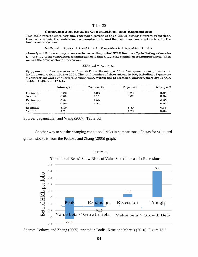
94

Table 30

Source: Jagannathan and Wang (2007), Table XI.

Another way to see the changing conditional risks in comparisons of betas for value and

growth stocks is from the Petkova and Zhang (2005) graph:

Figure 25

"Conditional Betas" Show Risks of Value Stock Increase in Recessions

Source: Petkova and Zhang (2005), printed in Bodie, Kane and Marcus (2010), Figure 13.2.

-0.33

-0.15

0.05

0.4

-0.4

-0.3

-0.2

-0.1

0

0.1

0.2

0.3

0.4

0.5

Peak Expansion Recession Trough

Bet

a of

HM

L p

ortf

olio

Value beta < Growth Beta Value beta > Growth Beta

95

In their testing results, Jagannathan and Wang (2007) find that the CCAPM performs as

well as, if not better than, the Fama-French three factor model in explaining cross-sectional

return differences among the 25 F-F portfolios sorted by size and book/market, using the year-

over-year fourth quarter consumption growth rate. In addition, the contraction beta is tested to be

more significant than expansion beta. Both findings support their hypothesis. Results are in the

following graphs:

Figure 26

Source: Jagannathan and Wang (2007).

The Jagannathan-Wang discretionary consumption decision model was motivated by

several important prior empirical tests, including conditioning, long-run risk and ultimate

consumption, as all of these models take into consideration the large errors in estimating short-

term consumption data and the discretionary psychology involved in consumption decision

making. As they point out, discretion is perhaps less consistent with Constantinides (1990) and

Campbell-Cochrane (1999) habit formation models, as consumption is likely less dependent on

the historical levels if more discretion is taken to review the decision. They reconcile the two

effects and show that the habit formation effect is dominated by the classic consumption beta in

asset pricing when the time between consumption decisions increases. However, this analysis is

based on the assumption of simultaneous and infrequent decision making of all consumers,

96

which is exogenous to the model and requires scrutiny. When a high implied risk aversion

parameter is found, they attribute it to the lack of realism of the assumption that consumers

simultaneously make choices only once a year. Overall, the Jagannathan-Wang paper added to

the string of significant papers that found consumption-based asset pricing, based on alternative

specifications of individuals’ consumption and portfolio choices, is able to explain cross-

sectional returns and the Fama-French size and book/market anomalies. However, the different

specifications lead to different economic understandings of the causal behavior generating the

observed returns.

XI. Long-Run Risks. Bansal-Yaron (2004)

In another major second generation consumption-based asset pricing model, 25+ years

after the original Consumption CAPM derivations, Bansal and Yaron (BY, 2004) developed a

model of “long run risks” in consumption growth. This has been an influential version of

consumption-based asset pricing for the past decade, spawning a substantial amount of additional

research. Their key innovations are: (1) to model expected consumption and dividend growth

rates as containing a small, persistent long-run predictable component, and (2) to model

changing volatility of consumption growth rates. They use Epstein and Zin’s (1999) forward-

looking preferences, which are recursive and exhibit time complementarity for consumption.

With regard to the modeling of a small, persistent long-run fluctuation in consumption

growth rates, Bansal and Yaron note that Shephard and Harvey (1990) show that in finite

samples, it is very difficult to distinguish between a purely i.i.d. process and one that

incorporates a small persistent component. While it is hard to distinguish econometrically

between the two alternative processes, the asset pricing implications across them are very

different. Bansal and Yaron observe that: “If, indeed, news about consumption has a nontrivial

impact on long-term expected growth rates or economic uncertainty, then asset prices will be

fairly sensitive to small growth rate and consumption volatility news. … For these channels to

have a significant quantitative impact on the risk premium and volatility of asset prices, the

persistence in expected growth rate has to be quite large, close to 0.98.” They show that their

combination of assumptions for consumption and dividend growth rates, which incorporate the

97

fluctuating persistent component, are consistent with the historic data and helps them explain

several of the literature’s puzzling aspects of asset price levels and fluctuations.

The Epstein-Zin preferences assumption drives a wedge between the elasticity of

intertemporal substitution (EIS) and relative risk aversion (RRA), which allows separate

modeling of each. Flexibility in fitting EIS to a high level (EIS=1.5) allows them to match the

low level of real short-term interest rates. Flexibility in fitting RRA to a relatively high level

(RRA=10) allows them to fit the relatively large risk premium on equities. Their modeling of

changing conditional volatility of the growth rate of consumption across time allows them to

model time-varying risk and risk premia. As shown by Bansal, Khatchatrian and Yaron (2002)

and confirmed in this paper, there is a significant negative correlation between price-dividend

ratios and consumption volatility. When consumption volatility is high, stock prices are low in

relation to dividends. They note that “about half of the volatility of the price-dividend ratios in

the model can be attributed to variation in expected growth rates, and the remaining can be

attributed to variation in economic uncertainty.”

Some of the specifics of Bansal and Yaron’s LLR model are as follows. Defining

consumption growth as gt , dividend growth as gd,t, and letting xt be the small, predictable

component of consumption growth, they specify that (eq. 4, p. 1485):

The following table shows the fit of Bansal and Yaron’s model with the statistical properties of

historic real consumption growth:

(71)

98

Table 31

Source: Bansal and Yaron (2004), Table I.

From the table, comparing the historic statistics with the means from simulations of the

LLR model, we see that the fit of consumption volatility and autocorrelation is quite good, on

average. The variance ratio statistics for both the data and the model are all above 1.0 for the

data shown (up to 10 years), which is consistent with positive autocorrelation in consumption

growth and persistent shocks, as the ratio would be 1.0 and variance would grow proportionally

through time, absent those effects. However, note that the 10-year variance ratio in the historic

data is less than the 5-year variance ratio (as in Cochrane (1988)), whereas the B-Y long run risk

model has the variance ratio continuing to increase from 5 to 10 years out. Perhaps at some

point, mean reversion of real consumption growth sets in (which seems quite plausible) and

offsets the effects of the persistent shocks. This long-run risk model would likely miss that

effect.

99

Bansal and Yaron’s model for the time-varying variance of real consumption growth has

both a purely random component and a mean reverting component, with υ1 describing the speed

of mean reversion:

The risk premium comes as a compensation for three consumption risks: short-run, long-

run and volatility risk. Time-variation in the risk premium is governed by the conditional

variance of consumption growth (i.e., it is high when current volatility is high). With fluctuating

economic uncertainty, as well as the persistent growth shocks, Table 32 shows that Bansal and

Yaron’s long run risk model can replicate historic data quite well for many key asset market

returns when constant relative risk aversion is between 7.5 and 10:

Table 32

Source: Bansal and Yaron (2004), Table 4.

Another nice feature of Bansal and Yaron’s long run risks model is that it is able to broadly mimic the

predictability of returns, growth rates and price/dividend ratios, as shown in the next table:

(72)

100

Table 33

Source: Bansal and Yaron (2005), Table VI.

Bansal and Yaron observe that “The model can justify the equity premium, the risk-free

rate, the volatility of the market return and the price-dividend ratio. As in the data, dividend

yields predict returns and the volatility of returns is time-varying.” Three critical observations

are: (1) the number of tuning parameters is so large that they have considerable flexibility to

overfit the data, (2) their model requires constant relative risk aversion near 10 to duplicate the

data, which is relatively high, and (3) EIS needs to be large (1.5) to replicate the negative

correlation between consumption volatility and price-dividend ratio present in the data, which is

well above the EIS indicated by Vissing-Jorgensen’s (2002) research. Nonetheless, the fact that

they are able to provide results that provide an economic rationale for the equity premium puzzle

and duplicate a 6% risk premium, while having a low risk free rate and reasonable volatility, is

quite impressive. To be able to get these results with simply a small persistent growth term and

with time-varying volatility is surprising. Subsequent sections each have articles on the Bansal-

Yaron (2004) long-run risk model, as it continues to be one of the most impactful articles in

consumption-based asset pricing in the past decade.

101

XII. Cash Flow Betas: Consumption Risk vs. Market Risk

In their original derivation of the Consumption CAPM, Breeden and Litzenberger (BL,

1978) realized that measuring consumption betas from cash flows such as dividends or profits,

rather than from stock market prices and returns, could be useful in practice, as they noted:

“…the correct beta to be used in finding the risk-adjusted discount rate is the cash flow’s

volatility with respect to aggregate consumption, not with respect to the market portfolio.

For capital budgeting, these betas may be easier to estimate than “market” betas, since the

cash flows of many projects may be more closely related to GNP or aggregate

consumption than to the level of the market portfolio.” (BL 1978, p. 646)

Breeden (1989b) presented OLS regression results that confirmed this intuition by

estimating (unconditional) cash flow betas, using National Income and Product Accounts (NIPA)

annual data for real growth of profits, dividends and cash flows versus real market returns and

real consumption growth, (separately for total and nondurables and services consumption):7

Table 34

Breeden (1989b), Table 3.

In Breeden (2005), unconditional consumption and market betas for various industries

were presented, based upon 2-quarter changes in real profits over the 1948-2004 period:8

7 Note that Durbin-Watson statistics were approximately 1.6 to 1.9 in these regressions, with Dividends having the

lowest DW, given their stickiness. Note also that the Net Cashflow results were dominated by an outlier in 1933.

Breeden (2005) presented similar results with data through 2003 in his handout as the Distinguished Speaker at the

Western Finance Association meetings in Portland, Oregon in June, 2005. 8 To deal with negative profits or near-zero profits in certain industries, actual calculations were of changes in real

profits, divided by prior quarter employee compensation, then divided by overall average profits/compensation.

102

Table 35

The consumption betas from profits are quite different from betas estimated with stock

market returns, though they are significantly correlated. Profits do reflect leverage and are

highly volatile. For the U.S. Total, profits move by 4.3% when NDS real consumption growth

moves by 1%, and motor vehicles, which are quite cyclic, have 1-year profits growth that move

by 15.1% then (or 3.51 times as much as aggregate profits move). Motor vehicles, durables and

wholesale trade all have stock market betas that are quite similar, between 1.08 and 1.16, but

their relative profit betas are 3.51, 2.42 and 0.84, respectively. Utilities, oils and banks had low

consumption betas of profits, but higher stock market betas. Banks’ profit betas should increase

in more recent samples that include the recent Great Recession. Breeden (1989b) also found that

industry profits were often mean-reverting over 3-5 years, which makes sense, given competition

and freedom of entry. Very high profits entice additional supplies and competition. Stock

market betas and dividends should pick up these longer term effects.

Updated annual data for 1930-2012 for the relation of real profits changes to real S&P

500 returns and to the growth rate of real, nondurables and services consumption are in Figures

27 and 28. It can be seen that annual profit growth is more related to consumption changes than

to stock returns.

Cash Flow Risks Ranked by Industry: Consumption Betas vs. Market Betas

Nonoverlapping 2-Quarter Real Percentage Changes in Real Profits, 1948-2004.

S&P500 betas are K. French Real Industry Returns vs. S&P500 Real Return

Profit Beta, Real 2Q, vs. Relative Consumption Beta Industry Stock Beta vs.

Industry %Chg Real NDS Consumption (Industry divided by US Total) Real Return on S&P 500

Motor Vehicles 15.1 3.51 1.08

Durables 10.4 2.42 1.16

Retail Trade 9.2 2.14 1.09

Construction 8.5 1.98 1.23

Wholesale Trade 3.6 0.84 1.10

Food & Beverage 2.9 0.67 0.84

Banks 1.7 0.40 1.03

Oil 1.6 0.37 0.76

Utilities -1.0 -0.23 0.61

U.S. Total 4.3 1.00 1.00

Source: Breeden (2005).

103

Figure 27 Figure 28

Note: When real total consumption growth is used, instead of NDS consumption, R

2=.51 and t-statistic

for the slope is 8.6.

In a modern, econometrically stronger test of whether consumption risks of cash flows

are helpful measures of risk, Bansal, Dittmar and Lundblad (BDL, 2005) examined dividends

and share repurchases versus real NDS consumption growth for 30 portfolios: 10 decile

portfolios ranked by size, book/market and momentum, respectively. They say (p. 1640): “We

show that the cross-sectional dispersion in the measured cash flow beta explains approximately

62% of the cross-sectional variation in observed risk premia. Further, the estimated market price

of consumption risk is sizable, statistically significant, and positive in all cases.” They are able

to duplicate much of the spread in mean returns of the extreme momentum portfolio (winner

minus loser) and similarly defined size and value portfolios, using quarterly data from 1967 to

2001. Means and standard deviations of returns for the 30 portfolios are in Table 36. They

display the well-known effects during this period that small stocks, high book/market, and

positive momentum portfolios have the highest mean returns:

104

Table 36

Source: Bansal, Dittmar, Lundblad (2005), Table I.

The estimated cash flow (dividend) growth rates for the 30 portfolios are interesting and

in the next table:

Table 37

Source: Bansal, Dittmar, Lundblad (2005), Table II.

Small firms having the highest cash flow growth is as expected. However, high book/market

firms, “value stocks,” display higher growth rates than the “growth stocks,” which helps BDL duplicate

the value effect. Key to BDL being able to duplicate momentum effects is the result that the high positive

momentum stocks display faster cash flow growth, while the negative momentum stocks have negative

growth, perhaps not surprising, but interesting.

Summary Statistics: Portfolio Returns for Size, Book/Market, Momentum Decile Portfolios

Quarterly returns: 1967-2001

Size Mean Std.Dev Book/Market Mean Std.Dev Momentum Mean Std.Dev

S1 (Small) 0.023 0.137 B1 Low 0.015 0.106 M1 (Losers) -0.010 0.154

S2 0.023 0.127 B2 0.020 0.096 M2 0.007 0.119

S3 0.023 0.120 B3 0.021 0.092 M3 0.012 0.109

S4 0.023 0.117 B4 0.022 0.092 M4 0.020 0.094

S5 0.024 0.111 B5 0.020 0.080 M5 0.014 0.087

S6 0.021 0.105 B6 0.023 0.081 M6 0.016 0.088

S7 0.022 0.104 B7 0.024 0.084 M7 0.020 0.089

S8 0.022 0.100 B8 0.026 0.084 M8 0.024 0.083

S9 0.021 0.091 B9 0.027 0.089 M9 0.028 0.093

S10 (Large) 0.018 0.083 B10 (High) 0.033 0.103 M10 (Winners) 0.036 0.114

Summary Statistics: Portfolio Real Cash Flow (Dividend) Growth

Size Mean Std.Dev Book/Market Mean Std.Dev Momentum Mean Std.Dev

S1 (Small) 0.011 0.055 B1 Low -0.001 0.040 M1 (Losers) -0.039 0.228

S2 0.010 0.039 B2 0.002 0.051 M2 -0.019 0.130

S3 0.008 0.038 B3 0.003 0.072 M3 -0.009 0.112

S4 0.007 0.039 B4 0.005 0.070 M4 -0.002 0.080

S5 0.007 0.040 B5 0.003 0.047 M5 -0.003 0.090

S6 0.003 0.030 B6 0.006 0.032 M6 0.002 0.075

S7 0.005 0.037 B7 0.005 0.034 M7 0.004 0.104

S8 0.004 0.065 B8 0.009 0.040 M8 0.012 0.092

S9 0.002 0.042 B9 0.008 0.046 M9 0.021 0.122

S10 (Large) 0.000 0.018 B10 (High) 0.011 0.089 M10 (Winners) 0.028 0.178

105

To estimate consumption risks, BDL use two alternative methods. First, they estimate γi

to be the “projection of portfolio-specific dividend growth on the moving average of

consumption growth,” using an 8-quarter moving average of prior consumption growth with a

lag length of 4 quarters, which is akin to Parker and Julliard’s (2005) 11-quarter consumption

calculations for “ultimate” consumption betas. Secondly, they estimate the sensitivity of the

innovation in dividend growth rates to the estimated innovation in consumption growth, which

gives their βig estimates in Table 38:

Table 38

Source: Bansal, Dittmar, Lundblad (2005), Table III.

SE R2 SE SE R

2 SE SE R2 SE

S1 1.2 2.9 0.003 2.4 4.5 B1 3.0 2.9 0.039 5.9 5.1 M1 -8.9 7.5 0.010 -12.8 12.8

S2 2.8 2.5 0.034 6.1 4.7 B2 -3.4 2.3 0.029 -3.6 4.1 M2 -1.4 4.8 0.001 0.2 8.2

S3 0.8 1.9 0.003 1.4 3.3 B3 0.02 2.4 0.000 0.4 4.2 M3 -1.7 5.4 0.002 1.3 9.0

S4 0.8 1.4 0.003 1.0 2.1 B4 -0.3 2.8 0.000 -0.9 4.8 M4 -0.5 2.5 0.000 -0.1 4.1

S5 0.8 1.5 0.002 1.7 2.5 B5 0.5 1.8 0.001 0.5 3.3 M5 -0.7 3.8 0.000 2.0 5.6

S6 2.0 1.1 0.028 3.8 2.2 B6 1.7 1.5 0.018 3.5 2.9 M6 2.5 2.0 0.007 3.7 3.8

S7 1.4 1.6 0.009 2.5 2.8 B7 0.8 1.1 0.003 2.2 2.2 M7 4.2 4.1 0.010 5.0 7.0

S8 1.1 1.7 0.002 2.8 2.9 B8 4.4 1.7 0.076 7.0 3.1 M8 6.3 3.5 0.030 7.4 6.4

S9 1.1 1.0 0.004 2.2 1.7 B9 4.7 3.1 0.071 10.3 4.9 M9 7.6 5.8 0.025 11.6 10.0

S10 1.1 0.7 0.022 2.7 1.2 B10 8.4 4.1 0.057 16.7 7.7 M10 11.6 5.7 0.027 15.2 12.4

Source: Bansal, Dittmar, Lundblad (2005). Table III.

𝛾𝑖 𝛽𝑖.𝑔 𝛾𝑖 𝛽𝑖.𝑔 𝛽𝑖.𝑔𝛾𝑖

106

There is some instability in these cash flow consumption risk estimates, and there is no

clear relation of beta estimates to size. However, for book/market portfolios, the value stocks do

have noticeably higher cash flow consumption betas than do the growth stocks, and the high

momentum stocks also have higher cash flow consumption betas than the negative momentum

stocks. Note that the standard errors are high relative to risk estimates, and R2 are very low. So it

is surprising that the estimated cross-sectional relations for returns versus these cash flow

consumption risks show such a strong relationship. The cross-sectional evidence (using GMM

estimates) is in Table 40, with cash flows measured in 2 ways and risks measured in 2 ways:

Table 39

Source: Bansal, Dittmar, Lundblad (2005), Table IV. GMM estimates.

Bansal, Dittmar and Lundblad’s table shows a significant cross-sectional relationship of

risk premiums with cashflow consumption betas from dividends, which explains 62% to 66% of

return premiums. With repurchases added, the relationship is a bit weaker, but still strong, with

R2 ranging from 46% to 61%. All in all, this is quite a good showing for cash flow consumption

betas. Note that BDL confirmed the Lettau and Ludvigson result that unconditional consumption

betas fit returns very poorly.

Hansen, Heaton and Li (HHL, 2008), in the colorful title “Consumption Strikes Back?

Measuring Long Run Risk,” carefully developed an interesting model that contained both short-

Cross-Sectional Evidence: Returns vs. Cash Flow Consumption Betas

λ0 Std Error t-stat λc Std Error t-stat R2

Coeff. 1.754 (0.815) 2.15 0.177 (0.072) 2.46 0.663

Coeff. 1.658 (0.837) 1.98 0.118 (0.027) 4.37 0.620

Coeff. 1.741 (0.851) 2.05 0.166 (0.057) 2.91 0.607

Coeff. 1.697 (0.859) 1.98 0.105 (0.030) 3.50 0.456

Panel A:Dividends

Independent Variable Is γi

Independent Variable Is βi,g

Panel B:Dividends Plus Repurchases

Independent Variable Is γi

Independent Variable Is βi,g

107

term, transitory shocks and long-term, permanent shocks in an economy of consumers with

Epstein Zin and Weil preferences. Impulse response functions for both shocks are in Figure 29:

Figure 29

Source: Hansen, Heaton and Li (2008), Figure 3.

HHL model corporate profits as being cointegrated with consumption and study the

valuation of growth and value stocks as an application of their model. The following figure

shows how differently cash flows of value and growth stocks move, relative to consumption:

Figure 30

Source: Hansen, Heaton and Li (2008), Figure 1.

108

While the return of value stocks over growth is well-known, the much greater long-run volatility

of value stocks’ performance in consumption units is quite noticeable. By contrast, movements

in growth stocks and the market portfolio are tame. As Hansen, Heaton and Li observe (p. 261):

“We find that the cash flows of value portfolios exhibit positive comovement in the long run

with macroeconomic shocks, whereas the growth portfolios show little covariation with these

shocks. Equilibrium pricing reflects this heterogeneity in risk exposure: risk-averse investors

must be compensated to hold value portfolios.” Using data for the Fama-French (1992) high

book/market portfolio 5 versus that for the growth portfolio 1, they graph the impulse responses

of cash flows of both to a permanent shock in consumption as in the next figure:

Figure 31

Source: Hansen, Heaton and Li (2008), Figure 8.

This shows that consumption shocks have transitory impacts on growth stock

performance, but permanent impacts on value stocks, leading to the value premium.

109

In another significant article with conditional consumption betas, Bansal, Dittmar and

Kiku (BDK, 2009) found that betas generated by an error correction, vector autoregressive (EC-

VAR) model with cointegration restrictions between dividends and consumption can explain

cross-sectional differences at many horizons, outperforming the model without the cointegration

restriction. As they say (p. 1344), “…the deviation of the level of dividends from consumption

(the error correction variable) is important for predicting dividend growth rates and returns at all

horizons.” And then they say (p.1344): “Imposing cointegration, we are able to predict on

average 11.5% of the variation in one-year returns, compared to 7.5% when we do not impose

cointegration. This difference is even starker at longer horizons: at the 10-year horizon, the EC-

VAR specification results in an average 44.0% adjusted R2, compared to 9.9% for the standard

growth-rate VAR specification.” This predictability evidence, they claim, has important

implications for measuring return innovations and, consequently, conditional consumption betas.

They argue that the error correction term of the cointegrated VAR contains important

information and can predict future dividend growth by conditioning, which translates into

longer-term return predictability. Their empirical results suggest that return predictability

increases more than dividend predictability does when adding the EC term into the VAR model.

Please note that Bansal, Dittmar and Kiku (2009) assume that all individuals are identical

and have a standard, time-additive power utility function with everyone having the same CRRA.

This is a special case of the original derivations of the CCAPM in the late 1970s (See Section II),

some of which were derived for heterogeneous individuals and more general time-additive utility

and do not assume that anyone has CRRA utility. So all of the results and insights of those

original models must apply to this one and the contributions here are empirical, not theoretical.

Bansal, Dittmar and Kiku use annual data from 1929-2002, quite a different sample than for

Bansal, Dittmar, Lundblad’s 1963-2001 quarterly sample. Their data for dividends and returns

are in the next table for dividend growth and returns for size and book/market decile portfolio:

The BDK longer-term calculations use more stable annual data and appear to have more

continuous estimated movements in returns and risk measures for size and book/market

portfolios than in BDL (2005):

110

Table 40

Source: Bansal, Dittmar, Kiku (2009), Table 1. 1929-2002 annual data.

As BDK observe, “Cointegration implies that the dividend growth rates are predicted by

the cointegrating residuals. That is, the current deviations of an asset’s cash flows from their

long-run relation with consumption should forecast the dynamics of dividend growth rates while

dividends are moving back toward equilibrium.” As dividends are a key element in investment

returns, especially in the longer term, this may also translate into return predictability.

Comparisons of the predictability of dividend growth and stock returns for the 20 portfolios with

an error-correction vector autoregression (EC-VAR) with a standard VAR model are in Tables

41 and 42, respectively:

111

Table 41

Source: Bansal, Dittmar, Kiku (2009), Table 3.

Table 42

Source: Bansal, Dittmar, Kiku (2009), Table 4.

112

Examining Tables 42 and 43, we see the following: the cointegrated model, EC-VAR, is

better than the standard VAR in the short and medium term, which makes sense as the error

correction model picks up transitory variation in dividend growth rates. With regard to return

predictability, the cointegrated model, EC-VAR, does has much better predictive accuracy,

causing BDK to observe that (p. 1358): “…the cointegrating residual, included in the error-

correction specification, contains distinct information about future returns beyond that in the

growth-rate-based model.” As return innovations differ across the two models, consumption

betas will also differ between the models. Table 44 gives the estimated consumption betas in the

cointegrated model. Notice the large differences in EC-VAR versus the VAR estimates:

Table 43

Source: Bansal, Dittmar, Kiku (2009), Table 6.

113

A close examination of Tables 42 and 43 confirm that : “Neither the unconditional betas

nor those based on the VAR reflect the cross-sectional differences in mean returns on size and

book-to-market-sorted portfolios.” Table 44 gives the one-step GMM estimates of the market

prices of risk that are jointly estimated with the time-series parameters. The R2 values for the

error-correction model are very high, at 73% to 84%, in contrast to the standard VAR results.

Also, the estimated prices of risk are all estimated as 2 to 3 times their standard errors.

Table 44

Source: Bansal, Dittmar, Kiku (2009), Table 7.

Graphs of the very strong 1-year and long-term fits of the EC-VAR model are in Figure 32:

Figure 32

Source: Bansal, Dittmar, Kiku (2009). Figure 2.

114

Strong results with consumption betas require modeling of conditional consumption betas.

From the works of Lettau and Ludvigson (L-L, 2001b), Bansal, Dittmar, Lundblad (2005),

Jagannathan and Wang (2007), and Bansal, Dittmar, Kiku (2009), we learned that it is very

important to have a conditioning variable for consumption betas, as they change over time and

economic states. L-L conditioned upon cay, their variable that represents consumption’s

deviations from a broad wealth variable (stocks, bonds and real estate) that also includes

capitalized wage income. In contrast, J-W quite reasonably conditioned upon NBER-designated

recession and expansion periods. Bansal, Dittmar and Kiku conditioned upon the deviations of

dividends from their long-term trend with consumption.

XIII. More Consumption-Based Pricing Research in the Past Decade

The literature on consumption-based asset pricing is vast and burgeoning, so it is

impossible to properly present and review all of the excellent research in a single article. In this

section, we examine additional articles that were published in the past decade, 2004-2014.

A: Risks of Rare Disasters

Almost two decades after Rietz’s (1988) classic work on a disaster risk explanation of

Mehra and Prescott’s (1985) equity premium puzzle, Barro (2006) and Barro and Ursua (2008)

and then Wachter (2013) gathered new data and built new models of the risks of rare disasters.

As Barro (2006, p. 823) said “I think that Rietz’s basic reasoning is correct, but the profession

seems to think differently…” and “… the major reason for skepticism about Rietz’s argument is

the belief that it depends on counterfactually high probabilities and sizes of economic disasters.”

Barro, using data from Maddison (2003) (with some corrections), found 60 instances among 20

OECD countries of peak-to-trough declines in real per capita GDP of 15% or more in the

twentieth century. The average decline was 29% of GDP. Barro computes the probability of

such a -15% or more disaster to be 1.7% per year, on average, using data for the 20 OECD

countries for which there was data. Barro finds the frequency distribution of contractions to be

as in the following graph:

115

Figure 33

Source: Barro (2006), Figure I.

Barro also compute the combination of disaster probability and relative risk aversion that

would explain the observed equity risk premium. The result is in the following graph, where b is

the loss that occurs in a typical disaster, which is simulated to be a 25% to 50% decline in real

GDP, peak to trough. Note that CRRA = 4.3, a not implausible level of risk aversion, combined

with the historic probability of 1.7% per year, fits the historic equity risk premium.

Figure 34

Source: Barro (2006), Figure II.

116

More recently, Wachter (2013) pointed out that Rietz’s and Barro’s models would have

stock market volatility equal to the volatility of dividends, which is so low as to not be realistic.

Wachter shows that modeling the probability of a consumption disaster as time-varying can

solve the problem. As she says (p. 987), “The possibility of this poor outcome substantially

increases the equity premium, while time variation in the probability of this outcome drives high

stock market volatility and excess return predictability.” Wachter’s specific model for the

stochastic process for aggregate consumption is as follows:

Thus, Wachter has a mixed jump-diffusion process. In normal times, when no disaster takes

place, consumption follows a continuous diffusion process. Disasters are captured by the

Poisson jumps downward in consumption, where: “Roughly speaking, λt can be thought of as

the disaster probability over the course of the next year.” (p. 991)

The equity premium in Wachter’s model is different from previous models, reflecting the

presence of disaster risk, and then also reflecting the time variation in disaster risk, as follows

(her eq. 28):

Note that the second term produces time variation in the equity premium that reflects

changes in the disaster jump intensity, λt, while the third term gives the impact of a static amount

of rare disaster risk.

(73)

(74)

(75)

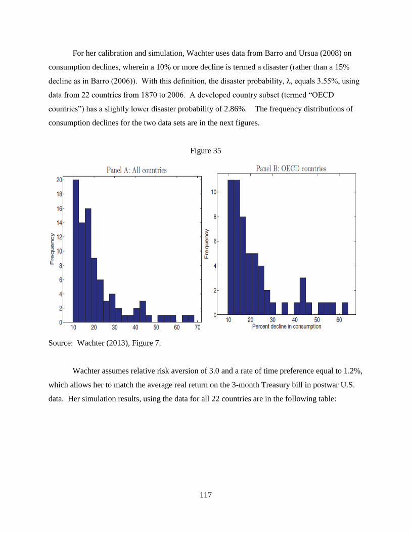
117

For her calibration and simulation, Wachter uses data from Barro and Ursua (2008) on

consumption declines, wherein a 10% or more decline is termed a disaster (rather than a 15%

decline as in Barro (2006)). With this definition, the disaster probability, λ, equals 3.55%, using

data from 22 countries from 1870 to 2006. A developed country subset (termed “OECD

countries”) has a slightly lower disaster probability of 2.86%. The frequency distributions of

consumption declines for the two data sets are in the next figures.

Figure 35

Source: Wachter (2013), Figure 7.

Wachter assumes relative risk aversion of 3.0 and a rate of time preference equal to 1.2%,

which allows her to match the average real return on the 3-month Treasury bill in postwar U.S.

data. Her simulation results, using the data for all 22 countries are in the following table:

118

Table 45

Source: Wachter (2013), Table II.

Note that Wachter’s “Conditional” results, when there was no disaster, match the U.S.

postwar data quite well. However, the “Population” results, which include a normal fraction of

disasters, have consumption volatility over 6%, in contrast to the 2% volatility with no disasters.

Volatility of dividends depends also greatly upon whether or not there was a disaster in the

sample period. In summary, Wachter’s mixed jump-diffusion model does a good job at

mimicking historic data when there are no disasters, and shows what data should look like over

the very, very long term when we have a normal (small) proportion of disasters in the sample.

B. Predictability of Dividends and Returns

In 2005, Lettau and Ludvigson, modeled consumption, stock dividends and labor income

(dividends from human capital) as having a three-way cointegrated relationship, much as in their

2001 article that developed cay, but with asset wealth being replaced by dividend growth via the

Campbell-Mankiw (1989) derivation. In the post-World War II era, dividend yield has been a

less useful predictor of stock returns. Lettau and Ludvigson argue that this is in part the result of

the offsetting effects of dividend growth and equity risk premiums. In a recession, risks likely

increase, dividend yields increase as stock prices fall more than dividends, and projected returns

119

on stocks increase to compensate for higher risk. However, if dividends have fallen, expected

dividend growth may increase, partially offsetting the effects of the higher risk premium. Lettau

and Ludvigson find that this positive covariation of dividend growth with market risk premiums

masks greater volatility in both in the post-War period. In the pre-war era, they find no evidence

of this cointegrating relation and find little predictive power in the pre-War data.

Santos and Veronesi (2006) have a straightforward, but powerful model of time variation in the

equity risk premium and changes in conditional risks of assets. They model consumer spending as being

composed of two parts – the part funded by labor income and the part funded by financial assets, such as

stock returns. Their hypothesis is that when labor income provides a larger fraction of financing for

consumption (and stock returns provide a smaller portion), stock returns will be less correlated with

optimal consumption at those times and will earn smaller risk premiums due to their smaller consumption

betas then. In contrast, when stocks provide a large fraction of funds for consumption, covariance of

consumption with stock returns increases and risk premiums on stocks should increase. Thus, as the ratio

of labor income (compensation of employees data) to consumption (shown in Figure 36) increases, the

equity risk premium should fall, a negative relationship.

Figure 36

Santos and Veronesi (2006), Figure 1.

120

In the graph, compensation of employees, the dotted line, is the broader measure of labor

income, including bonuses, as well as wages and salaries. Note that in the sharp recessions in

1974/75 and 1981/82, the share of consumption paid for by labor income (which was quite high)

dropped sharply, so that paid by financial assets provided a larger fraction and the conditional

consumption beta of stocks and the time-varying risk premium should have increased. The next

graph compares visually the ability of the labor income share to (negatively) predict subsequent

4-year returns on equities, compared with the ability of dividend yields to do so:

Figure 37

Source: Santos and Veronesi (2006), Figure 2.

121

Statistics for the ability of the labor income/consumption ratio and the dividend yield ratio to

predict stock returns are in Table 46. The labor income/consumption ratio has greater ability to predict

returns than does dividend yield during the post-War period. Long-term (4-year) predictability is quite

high, with R2 = 0.42 for the labor income/consumption ratio, versus 0.14 for dividend yield. Combining

both predictors is better yet, with R2 = 0.57 over the 1948-2001 sample period, all statistically significant.

Table 46

Source: Santos and Veronesi (2006), Table 2.

Using the labor income/consumption ratio as a conditioning variable, much as Lettau and

Ludvigson (2001b) did with cay, Santos-Veronesi also get very positive results for the conditional CAPM,

in cross-sectional fits of returns of the 25 Fama-French portfolios sorted by size and book/market.

122

C. Durable Goods Consumption, Systematic Risk and Asset Pricing

Yogo (2006) did very interesting research on durables consumption flows, finding asset

pricing, risk measurement and risk premium results that were quite strong. This is especially

interesting, as so many researchers simply use the nondurables and services part of consumption

and exclude durables, due to the fact that only a portion of the durable is consumed annually (6%,

as estimated by the U.S. Bureau of Economic Analysis). Yogo found that the ratio of durables

consumption flows to nondurables and services is highly procyclic, with durables moving more

sharply up and down with the economy than NDS consumption. This seems plausible

introspectively, in that when individuals have moved up significantly in wealth or income, often

they buy nice durable goods and luxury items, such as cars, jewelry, or vacation homes and

control (reduce) marginal utility optimally in that way. Of course, in recessions, durables

purchases are sharply curtailed and households live off their old durables stocks. Thus, durables

spending could be quite an excellent signal of changes in marginal utility, which is indeed what

Yogo found. A graph of the ratio of Durables stocks to nondurables consumption is in Figure 33.

It shows the very procyclic nature described, as well as the increasing share of real durables

consumption in total consumption, in part responding to the relative price decline of durables.

The correlations of the three Fama-French factors with nondurables and durables

consumption with quarterly data from 1951 to 2001 are in the following table, along with mean,

volatility and autocorrelation statistics. Note that durables consumption growth is highly

autocorrelated, much more so than is nondurables (0.88 vs. 0.28). Correlations of durables

consumption growth with the stock market and SMB and HML factors are all low, and the

correlation of these quarterly changes with nondurables spending is only 0.19.

123

Figure 38

Source: Yogo (2006), Figure 1.

Table 47

Source: Yogo (2006), Table I.

Yogo provides first-stage GMM estimates of consumption betas of the 25 (5x5) Fama-

French portfolios sorted by size and book/market, as in Table 47. Note the much sharper

124

correspondence of stocks’ average excess returns between stocks’ betas with durables

consumption than with their betas with nondurables.

Table 48

Source: Yogo (2006), Table IV.

Graphically, the relation of cross-sectional returns vs. risks measured by market betas, the

Fama-French 3-factor model, nondurables consumption betas and durables are in Figure 39:

125

Figure 39

Source: Yogo (2006), Figure 4.

Interestingly, Yogo also has the consumption betas for various industries relative to

nondurables and durables, estimated by first stage GMM:

126

Table 49

Source: Yogo (2006), Table VII.

Note that value stocks (high B/M) have much higher durables betas than do growth stocks,

whereas the nondurables betas are not much different. This helps explain the ability of the durables betas

to do so well in explaining the cross-section of average returns.

Finally, Yogo also is able to demonstrate that durables can also model time variation in

the estimated equity premium, as durables move sharply down in recessions at a time when risk

and risk aversion cause the equity premium to surge, shown in Figure 40:

Figure 40

Source: Yogo (2006), Figure 5.

127

A weakness in Yogo’s model is that the implied level of relative risk aversion is

extremely high at CRRA=174. This high estimate is due to the significant risk premiums,

despite the very low volatility of durables consumption stocks and durables consumption flows.

Gomes, Kogan and Yogo (GKY, 2009) follow up on Yogo’s (2006) analysis of the

consumption of durable goods. An innovation for this article is their construction of better

industry classifications than the U.S. government provides, using the BEA’s input/output tables

for cash flows in the economy. GKY (2009, p. 943) document four new facts in the cross-

section of cash flows and stock returns: (1) cash flows of durable goods producers are more

volatile and are more correlated with aggregate consumption than are other industries, (2) returns

on the durable goods portfolio are higher and more volatile on average, (3) cash flows of

durable-good producers are conditionally more volatile when the durable expenditure/stock ratio

is low, which generally coincides with recessions, and (4) the returns on the durable goods

portfolio are more predictable. Supporting point (2), over the 1927-2007 period, a portfolio that

is long durable goods and short the services portfolio earned an average annual return over 4.0%.

Supporting (4), a portfolio that is long durables and short the market portfolio has

countercyclical expected returns, reliably predicted by the durables expenditure/stock ratio.

A key mechanism in the Gomes, Kogan, Yogo model is that (p. 944): “…a proportional

change in the service flow (or the stock) of durable goods requires a much larger proportional

change in the expenditure on durable goods.” They argue that: “the difference in the conditional

cash flow risk between durable-goods producers and nondurable-good producers is relatively

high when the existing stock of durables is high relative to current demand. This mechanism

leads to a testable implication that the durable expenditure-stock ratio predicts cross-sectional

differences in the conditional moments of cash flows and stock returns…” The next graph

shows the cyclical movements of the durable expenditure-stock ratio. Note the sharp drops in

the Great Depression, as well as in sharp recessions in 1974/75 and 1981/82.

128

Figure 41

Source: Gomes, Kogan, Yogo (2009), Figure 2.

GKY use the durables expenditure-stock ratio as a predictor variable for excess returns and Table

49 shows that it has performance that is comparable to that of aggregate dividend yield, especially in the

postwar period. Consistent with the conditionally higher expected returns in recessions, additional

results (not shown) confirm that cash flow risk and 5-year dividend growth risk are higher when the

durables expenditure-stock ratio is low, as in recessions. Thus, in summary, the Gomes, Kogan, Yogo

article demonstrates the greater cyclicality of durables and the potential use of the durables expenditure-

stock ratio as a conditioning variable for modeling risk changes in the economy.

129

Table 50

Source: Gomes, Kogan, Yogo (2009), Table 5.

D. Real Estate.

Piazzezi, Schneider and Tuzel (2007) examine housing and consumption and the

“composition risk” between housing and nonhousing consumption and its impact on asset pricing.

They argue several points for the importance of this split, both theoretically and empirically.

Perhaps the most persuasive result that they find is that individuals really dislike reducing

housing consumption (habit formation), so they only do that if circumstances are very bad. So,

when housing expenditures decline sharply in relation to other expenditures (the “housing share”

declines), the economic state is very poor, almost in an “extreme risk” situation. They observe

that (p. 532): “In our model, investors’ concern with composition risk implies that recessions are

perceived as particularly severe when the share of housing consumption is low.” Housing is a

necessity and people don’t reduce it unless circumstances are very bad and marginal utility is

very high. They further state (p. 540) that: “stocks have …especially low payoffs in severe

130

recessions, when housing consumption is relatively low (and α is high). This generates higher

equity premia than under the standard model.”

Movements in the expenditure share on housing services, α, are in Figure 43, comparing the

expenditure share (α) on nonhousing services in the years from 1929 to 2001 with dividend yield:

Figure 42

Source: Piazzezi, Schneider and Tuzel (2007), Figure 1.

During World War II, resources were devoted to the war effort, and housing investment declined

relative to defense needs and other consumer spending. Post-World War II, there was a large catch-up in

housing expenditures as soldiers returned home, and spending on housing services was very high

(nonhousing low) and then reverted more to its long-term fraction of consumption. After those moves,

spending on housing as a fraction of total consumption has not varied as much (1960-2007).

Piazzezi, Schneider and Tuzel make another significant point that: (p. 548) “… times

characterized by relatively little housing correspond to times when the volatility of shocks is

higher. In other words, times with little housing are times of high uncertainty.” And further,

they observe that: (p. 560) “Interestingly, the model implies that a macroeconomic variable, the

(nonhousing) expenditure share, αt, should be a good forecasting variable. Intuitively, the model

implies that αt is high in severe recessions, when expected excess returns are high.”

131

Table 51

Source: Piazzezi, Schneider, Tuzel (2007), Table 5.

E. Limited Participation

Malloy, Moskowitz and Vissing-Jorgensen (2009), following on Vissing-Jorgensen’s

(2002) significant work on limited participation with Consumer Expenditure Survey data (CEX)

in Section VII, examine the consumption of stockholders versus nonstockholders, as well as

consumption by the wealthiest 1/3 of stockholders, in the long-run risk context of Bansal and

Yaron (2004) and Hansen, Heaton and Li (2008). Using the CEX data, they estimate the

sensitivities of stockholder, top stockholder and nonstockholders to fluctuations in aggregate

consumption over horizons from 1 quarter to 6 years, as shown in the next table:

132

Table 52

Source: Malloy, Moskowitz and Vissing-Jorgensen (2009), Table 1.

They find that, for example, at a horizon of 4 years, nonstockholders’ real consumption

growth moves approximately 1-for-1 with aggregate real growth, whereas “All Stockholders”

move by 2.7 times as much and the wealthiest 1/3, “Top Stockholders,” move by 3.9 times as

much as the aggregate. There is no reason for the Euler equations for stocks to hold for

nonstockholders, whereas they should for stockholders, the results of stockholders, and

especially for the ones with the most invested. Given the much higher sensitivities to aggregate

consumption (picking up only systematic consumption fluctuations), MMV-J estimates of

relative risk aversion are much lower “at around 10” (p. 2427) and nearing a range that many

economists find more plausible.

MMV-J estimated consumption growth covariances of the 25 Fama-French portfolios

with the different groups’s consumption rates and found substantial differences, depending upon

whether Top Stockholders, Stockholders, or Nonstockholders’ consumption growth were used,

as shown in Table 50. Note the dispersion of consumption covariances (betas) between value

and growth portfolios for stockholders versus for nonstockholders. Using stockholder

consumption shows value stocks to have much higher consumption risk than for nonstockholders.

133

This makes the cross-sectional relation of average stock returns (using 1926-2004 data) to

consumption covariances (using the CEX data period 1982-2004) have a much better fit for

stockholders, (especially Top Stockholders), than for Nonstockholders, as shown in Figure 43.

Figure 43

Source: Malloy, Moskowitz and Vissing-Jorgensen (2009), Figure 1.

134

Table 53

Source: Malloy, Moskowitz and Vissing-Jorgensen (2009), Table III

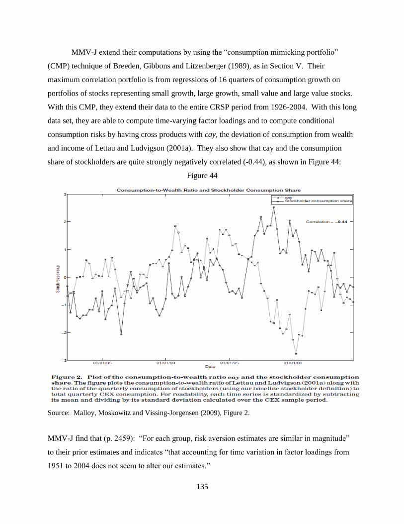
135

MMV-J extend their computations by using the “consumption mimicking portfolio”

(CMP) technique of Breeden, Gibbons and Litzenberger (1989), as in Section V. Their

maximum correlation portfolio is from regressions of 16 quarters of consumption growth on

portfolios of stocks representing small growth, large growth, small value and large value stocks.

With this CMP, they extend their data to the entire CRSP period from 1926-2004. With this long

data set, they are able to compute time-varying factor loadings and to compute conditional

consumption risks by having cross products with cay, the deviation of consumption from wealth

and income of Lettau and Ludvigson (2001a). They also show that cay and the consumption

share of stockholders are quite strongly negatively correlated (-0.44), as shown in Figure 44:

Figure 44

Source: Malloy, Moskowitz and Vissing-Jorgensen (2009), Figure 2.

MMV-J find that (p. 2459): “For each group, risk aversion estimates are similar in magnitude”

to their prior estimates and indicates “that accounting for time variation in factor loadings from

1951 to 2004 does not seem to alter our estimates.”

136

F. Foreign Exchange

Foreign exchange rates are quite important in the global economy. Their movements

make goods, services and labor cheaper or more expensive country by country (or for the

Eurozone) and, thereby, direct the flow of international investment and employment around the

world. When a country’s economy is strong, its unemployment rate drops, there is less slack in

the economy and its foreign exchange rate strengthens, which directs global investment to other,

less strong areas in the world. So there is and should be a positive correlation of foreign

exchange rates in a country with the country’s economic strength relative to other countries.

Lustig and Verdelhan (2007) examine data for 8 different currency portfolios, selected by

their interest rate spreads to the U.S. dollar, with portfolio 1 in low interest rate currencies, and

portfolio 8 in high rate currencies. Table 54 gives the rate spread to the US dollar, the average

rate of depreciation and average inflation rate in the countries over the 1953-2002 full sample, as

well as the post-Bretton Woods period of 1971-2002.

Table 54

Source: Lustig and Verdelhan (2007), Table 2.

Excess returns to the 8 portfolios show that the high rate currencies provided positive

excess returns, while the low rate currencies provided negative excess returns over both periods:

137

Table 55

Source: Lustig and Verdelhan (2007), Table 1.

If one considers investing in a currency, or playing a “carry trade” that is long a high

interest currency and short a low interest currency, one likely has a position that has nontrival

relative “consumption risk,” in that returns from the trade will depend upon the relative

performances of the economies, which most likely are reflected in their relative growths in real

consumption. Lustig and Verdelhan’s estimates of “unconditional” consumption betas show that

the higher interest rate currencies on average have higher consumption betas, whether betas are

measured relative to nondurables or relative to durables (as suggested by Yogo (2006)):

Table 56

Source: Lustig and Verdelhan (2007), Table 6.

138

Lustig and Verdelhan also do conditional estimates of betas, using the interest rate

differential as the sole conditioning variable. Thus, when risks get larger and a portfolio’s yield

spreads widen, estimated consumption betas increase, and when spreads shrink, risks decrease.

The authors observe (p. 102) that: “For every 4-percentage point reduction in the interest rate

gap, the nondurable consumption betas decrease by about 100 basis points.”

Table 57 gives the results for the estimated prices of consumption and market risks from

Fama-MacBeth regressions of cross-sectional returns on conditional betas for four consumption

models: (1) what they describe as the original CCAPM (using nondurables), (2) the Durables

Consumption CAPM of Yogo (2006) and (3) and (4) Epstein-Zin preference versions of both, as

well as for the Sharpe-Lintner CAPM and the Fama-French 3-factor and bond factor models:

Table 57

Source: Lustig and Verdelhan (2007), Table 11.

139

All four consumption-based models pass the chi-squared test and are not rejected, but

“only the models with durable consumption growth as a factor explain a large fraction of the

cross-sectional variation in returns.” Their benchmark model, using Durables Consumption

measures explains 54% to 64% of the variation, depending whether CRRA or the E-Z

preferences are used. Furthermore, “In this subsample, the CAPM explains none of the variation,

and the Fama-French factor models explain less than 18 percent…” Thus, as Lustig and

Verdelhan state (p. 89): “Because high interest rate currencies depreciate on average when

domestic consumption growth is low and low interest rate currencies appreciate under the same

conditions, low interest rate currencies provide domestic investors with a hedge against domestic

aggregate consumption growth risk.” For providing that consumption hedge, lower returns are

earned on average on the low interest rate currencies, even negative excess returns. It would be

interesting for researchers to also study the nonlinear risks, as it is plausible that there are

substantial nonlinear risks in currency movements.

140

XIV. Conclusion

In this article, we first reviewed the late 1970s major theoretical derivations that led to

consumption-based asset pricing models, one of the leading theories of asset pricing in the past

four decades. Next, we examined empirical testing and evolution of both theory and empirical

testing and of applications of consumption-based asset pricing, We began with individuals who

have heterogeneous time-additive utility functions and derived that their optimal responses to

market price signals should lead individuals to coordinate their consumption plans so that they

all have high consumption when aggregate real consumption increases and have low

consumption when aggregate real consumption decreases, leading us to the major aggregation

theorem. Even without effectively complete markets with a full set of hedges available, it was

shown that each individual would optimally choose a dynamic portfolio and optimal

consumption plan to achieve the maximum correlation possible of the individual’s consumption

with aggregate, per capita consumption. In that economy in the continuous-time model, the

Consumption CAPM was derived. Consumption betas were found to capture all of the risks and

risk premiums in Merton’s continuous-time Intertemporal CAPM, even with heterogeneous

individuals and incomplete markets. No assumption of identical investors or the existence of a

representative individual was required.

The 1980s empirical tests showed that there is a risk premium for consumption risk,

much as there was for market risk, but that the CCAPM was rejected, much like the original

market-oriented CAPM was. Assets’ conditional risk premiums were not found to be higher in

proportion to their conditional connsumption betas, as predicted by the CCAPM and the market-

oriented CAPM. An “equity premium puzzle” was identified in the 1980s, which identified a

mismatch between a relatively high risk premium on equities and very low volatility of real

aggregate consumption and relatively low correlation of equity returns with consumption

fluctuations. Researchers also found that models often had real riskless interest rates that were

higher than historical data, which gave rise to what some identified as a “riskless rate puzzle.”

141

Research proceeded along several dimensions, first by recognizing measurement of

consumption as an integral of daily/instantaneous consumption, versus stock returns as “point to

point returns.” Next, researchers noted the considerable noise in consumption measurements

versus consumers’ fundamental economic desires, reflecting often large but often transitory

impacts of weather, tax changes, labor strikes and such on income and consumption. Monthly

data for real consumption growth showed negative autocorrelation (presumably due to weather,

which can cause large monthly swings that dominate regression results), while quarterly,

semiannual and annual autocorrelations were positive, reflecting business cycle impacts. Tests

that relied upon monthly consumption growth estimates were found to be misleading relative to

subsequent results. Subsequent researchers found it more sensible to use 6-month or 2-quarter

returns, or 4-quarter returns, or even “ultimate consumption betas” that measured covariances

over almost 3 years (11 quarters).

Another dimension for research that was established in the late 1980s and early 1990s

was on models that exhibited time complementarity in utility for consumption, as in “habit

formation” models (which are backward looking, in that individuals’ utilities for current

consumption depended upon their habits formed from prior consumption levels). Another

popular model is of forward looking, recursive models of utility maximization (think of an

anticipated future inheritance, for example). The asset pricing implications of these more

general models allowed more flexibility in replicating financial and economic data and historic

means, volatilities and correlations. Perhaps not surprisingly, as they have more degrees of

freedom, these models were able to fit the data considerably better than prior models.

In the decade or so from 1991-2002, researchers used survey data compiled by the U.S.

Government on actual consumer spending by individual households to see how individual

consumption volatility differed from aggregate consumption volatility. Differences were

presumed to be due to “incomplete markets” for insuring major risks (such as for labor income),

as well as “limited participation,” in that some consumers simply did not invest in the stock

market. If they didn’t invest, their first-order conditions for an optimum likely were not met.

Thus, examining the consumption of stockholders versus that of nonstockholders yielded

considerable insights. First, it was found that volatility for a typical household was 5-10 times as

142

large as for aggregate real consumption, which helped to resolve the risk premium puzzle caused

in part by the low volatility of aggregate consumption. Secondly, it was found that both risk

aversion and elasticity of intertemporal substitution estimates (which closely related to riskless

interest rates) are much different between stockholders and nonstockholders and between

bondholders and nonbondholders.

These findings on incomplete markets and limited participation helped researchers to

resolve both the risk premium puzzle and the riskless rate puzzle. However, in the early 1990s,

two new puzzles were found in cross-sectional stock returns over long periods of time – the “size

effect” (small stocks earned higher returns than large stocks, beta adjusted) and the “value

premium” (where high book/market stocks, value stocks, earned more than growth stocks, beta

adjusted). Subsequent researchers tested their models on 25 (5x5) portfolios stratified by size

and value to see if they could explain these important results.

The 1990s and 2000s were periods of great progress in understanding and modeling

changing risks and changing risk premiums (“conditional risks”) in asset returns. It was shown

that in recessions, consumer spending was reduced towards “habit” levels and consumers

became very risk averse, (as they did not want to consume below their habit levels) just at a time

when risk was often very high. Thus, risk premiums skyrocketed in big recessions, as both risk

aversion became very high and risk was very high, and risk premiums were the product of the

two. Studying this, researchers found the clue to the value/growth puzzle, as value stocks were

found to have higher consumption risks when risk premiums were high, whereas growth stocks

had higher risks when risk was low, so the unconditional returns on value stocks should be

higher than for growth stocks, ceteris paribus. Thus, value and growth stocks had different

concavity or convexity, which relates very much to equilibrium returns on these investments.

With this new understanding and risk estimates, several researchers were able to explain the

value premium and the size premium.

Along with continuing development of the implications of habit formation on utility and

asset pricing, a new model of “long run risks” in consumption was developed in 2004. The

model is one where small movements in the changes in real consumption growth are so

143

persistent that they have really large implications for consumer spending long term and for asset

prices now, which anticipate long term effects. This model of long run risks has spawned a great

amount of research and has had a lot of empirical success.

At the present time, the “long-run risk model” and the “habit formation model” are the

two main empirical models in the consumption-based asset pricing space. Surely, each model

has its strengths, its weaknesses and its truths. Most of the theoretical insights still fit relatively

comfortably within the most general original models of asset pricing of the late 1970s. In this

article, with few exceptions, we have presented the outstanding research in this area in the past

four decades much as the authors did, often using their tables, graphs and descriptions for

authenticity and correctness. As well there should be, there is substantial academic debate about

the merits and challengers of the various models. We have not taken the time and space to

review the various claims and counterclaims by the authors of those competing models, but

instead refer the readers to the following articles by the authors: Campbell-Cochrane (2000),

Beeler-Campbell (2012) and Bansal, Kiku, Yaron (2012). In addition, two articles, Lewellen-

Nagel (2006) and Nagel-Singleton (2010), raised important concerns and objections to

significant amounts of the important research reviewed here and should also be examined

carefully, so that the reader more fully understands the larger issues of econometric testing of

consumption-based asset pricing models.

Consumption-based asset pricing has yielded many insights in the past four decades, both

theoretical and empirical. The financial economics literature has produced a vast body of

competing economic rationales for what earlier authors characterized as puzzles and paradoxes.

To borrow an econometric term: we have over-identified these puzzles and paradoxes. Further

research should attempt to integrate models and sort through them for the most important results

and develop tests based on different predictions of the models.

144

Literature Cited

Abel AB. 1990. Asset prices under habit formation and catching up with the Joneses. American

Economic Review, 80(2), 38-42.

Attanasio PO, Weber G, 1989, Intertemporal substitution, risk aversion and the Euler equation

for consumption, Economic Journal 99, 59-73.

Arrow KJ. 1964. The role of securities in the optimal allocation of risk-bearing. The Review of

Economic Studies, 31(2), 91-96.

Backus DK, Smith GW, 1993, Consumption and real exchange rates in dynamic economies with

non-traded goods, Journal of International Economics 35, 297-316.

Bansal R, Dittmar R, Kiku D. 2009. Cointegration and consumption risks in asset

returns. Review of Financial Studies, 22(3), 1343-1375.

Bansal R, Dittmar RF, Lundblad CT. 2005. Consumption, dividends, and the cross section of

equity returns. Journal of Finance, 60(4), 1639-1672.

Bansal R, Khatchatrian,V, Yaron A, 2002, Interpretable Asset Markets, NBER Working Paper

9383.

Bansal R, Kiku D, Yaron A. 2012. An empirical evaluation of the long-run risks model for asset

prices. Critical Finance Review, 1, 183–221.

Bansal R, Kiku D, Shaliastovich I, Yaron A. 2013. Volatility, the macroeconomy, and asset

prices. Journal of Finance, Forthcoming.

Bansal R, Yaron A. 2004. Risks for the long run: A potential resolution of asset pricing

puzzles. Journal of Finance, 59(4), 1481-1509.

Barro RJ, 2006, Rare disasters and asset markets in the twentieth century, Quarterly Journal of

Economics 121(3), 823-866.

Barro RJ, Ursua JF, 2008, Consumption disasters in the twentieth century, American Economic

Review 98 (2), 58-63.

Beeler J, Campbell J, 2012, The long-run risks model and aggregate asset prices: an empirical

investigation, Critical Finance Review 1, 141-182.

Bergman Y, 1985, Time preference and capital asset pricing models, Journal of Financial

Economics 14, 145-159.

145

Black F, Scholes M, 1973, The pricing of options and corporate liabilities, Journal of Political

Economy 81(3), 637-654.

Bodie Z, Kane A, Marcus AJ, 2011, Investments, 9th

edition. McGraw-Hill Irwin, New York.

Boguth O, Kuehn LA 2013. Consumption volatility risk. Journal of Finance, 68(6), 2589-2615.

Boldrin M, Christiano LJ, Fisher JD. 2001. Habit persistence, asset returns, and the business

cycle. American Economic Review, 91(1), 149-166.

Bollerslev T, Engle R, Woolridge J, 1988, A capital asset pricing model with time-varying

covariances, Journal of Political Economy 96, 116-131.

Brandt MW, Cochrane JH, Santa-Clara P, 2006, International risk sharing is better than you

think, or exchange rates are too smooth, Journal of Monetary Economics 53, 671-698.

Brav A, Constantinides GM, Geczy CC. 2002. Asset pricing with heterogeneous consumers and

limited participation: Empirical evidence, Journal of Political Economy, 110 (4), 793-824.

Breeden DT, 1977, Changes in consumption and investment opportunities and the valuation of

securities, unpublished Ph.D. Stanford University, December.

Breeden DT, Litzenberger RH. 1978. Prices of state-contingent claims implicit in option prices.

Journal of Business, 51(4), 621-651.

Breeden DT. 1979. An intertemporal asset pricing model with stochastic consumption and

investment opportunities. Journal of Financial Economics,7(3), 265-296.

Breeden DT. 1980. Consumption risk in futures markets. Journal of Finance, 35(2), 503-520.

Breeden DT. 1984. Futures markets and commodity options: Hedging and optimality in

incomplete markets. Journal of Economic Theory, 32(2), 275-300.

Breeden DT. 1986. Consumption, production, inflation and interest rates: A synthesis. Journal of

Financial Economics, 16(1), 3-39.

Breeden DT, Gibbons MR, Litzenberger RH. 1989a. Empirical tests of the consumption-oriented

CAPM. Journal of Finance, 44(2), 231-262.

Breeden DT, 1989b, Capital budgeting with consumption, presented at the French Finance

Association Annual Meetings, June. Renamed in 1991, Consumption and market risks of

corporate cash flows. Working paper, Duke Fuqua School of Business, June.

Breeden DT. 2004. Optimal dynamic trading strategies. Economic Notes, 33(1), 55-81.

146

Breeden DT. 2005. Western Finance Association 2005 Annual Meeting Distinguished Speaker

Handout, June 20, Portland Oregon.

Breeden DT. 2012. Consumption As A Leading Indicator. Working Paper, Massachusetts

Institute of Technology and Duke University, April.

Brunnermeier MK, Nagel S. 2006. Do wealth fluctuations generate time-varying risk aversion?

Micro-evidence on individuals' asset allocation. American Economic Review, 98(3), 713-736.

Campbell JY, 1987, Stock returns and the term structure, Journal of Financial Economics 18,

373-399.

Campbell JY. 1992. Intertemporal asset pricing without consumption data. American

Economic Review, 83(3), 487-512.

Campbell JY, 1996, Understanding risk and return, Journal of Political Economy 104, 298-345.

Campbell JY. 2000. Asset pricing at the millennium. Journal of Finance, 55(4), 1515-1567.

Campbell JY. 2003. Consumption-based asset pricing. Handbook of the Economics of

Finance, 1, 803-887.

Campbell JY, Cochrane JH. 1999. By force of habit: A consumption-based explanation of

aggregate stock market behavior. Journal of Political Economy, 107(2), 205-251.

Campbell JY, Cochrane JH, 2000, Explaining the poor performance of consumption-based asset

pricing models, Journal of Finance 55(6), 2863-2878.

Campbell JY, Mankiw NG, 1989, Consumption, income and interest rates: Reinterpreting the

time series evidence, NBER Macroeconomics Annual.

Campbell JY, Shiller RJ. 1988. The dividend-price ratio and expectations of future

dividends and discount factors. Review of Financial Studies, 1(3), 195-228.

Campbell JY, Vuolteenaho T. 2003. Bad beta, good beta. American Economic Review, 94(5),

1249-1275.

Chen N, Roll R, Ross SA, 1986, Economic forces and the stock market, Journal of Business

59(3), 383-403.

Cochrane JH. 1988. How big is the random walk in GNP. Journal of Political Economy, 96(5),

893-920.

Cochrane, JH, 1996, A cross-sectional test of an investment-based asset pricing model, Journal

of Political Economy 104(3), 572-621.

147

Cochrane, JH, 2005, Asset Pricing, Princeton University Press, Princeton.

Cochrane JH. 2008. The dog that did not bark: A defense of return predictability. Review of

Financial Studies, 21(4), 1533-1575.

Cochrane JH. 2011. Presidential address: Discount rates. Journal of Finance, 66(4), 1047-1108.

Cochrane JH. 2014. A Mean-Variance Benchmark for Intertemporal Portfolio Theory. Journal of

Finance, 69(1), 1-49.

Constantinides GM, 1990, Habit formation: A resolution of the equity premium puzzle, Journal

of Political Economy 98, 519-543.

Constantinides GM, Duffie D. 1996. Asset pricing with heterogeneous consumers. Journal of

Political Economy, 219-240.

Constantinides GM, Ghosh A. 2011. Asset pricing tests with long-run risks in consumption

growth. Review of Asset Pricing Studies, 1(1), 96-136.

Cox JC, Huang CF. 1989. Optimal consumption and portfolio policies when asset prices follow a

diffusion process. Journal of economic theory, 49(1), 33-83.

Cox JC, Ingersoll Jr JE, Ross SA. 1985. A theory of the term structure of interest

rates. Econometrica, 53(2), 385-407.

Cox JC, Ingersoll Jr JE, Ross SA. 1985. An intertemporal general equilibrium model of asset

prices. Econometrica, 53(2), 363-384.

Dotsey M, 1998, The predictive content of the interest rate term spread for future economic

growth, Federal Reserve Bank of Richmond Economic Quarterly vol. 84(3), 31-51.

Drechsler I, Yaron A. 2011. What's vol got to do with it. Review of Financial Studies, 24(1), 1-

45.

Duffee GR. 2005. Time variation in the covariance between stock returns and consumption

growth. Journal of Finance, 60(4), 1673-1712.

Duffie D. 2010. Presidential Address: Asset Price Dynamics with Slow‐Moving Capital. Journal

of Finance, 65(4), 1237-1267.

Duffie D, Huang CF. 1985. Implementing Arrow-Debreu equilibria by continuous trading of few

long-lived securities. Econometrica, 53(6), 1337-1356.

Dunn KB, Singleton KJ. 1986. Modeling the term structure of interest rates under non-separable

utility and durability of goods. Journal of Financial Economics, 17(1), 27-55.

148

Dusak K, 1973, Futures trading and investor returns: an investigation of commodity market risk

premiums, Journal of Political Economy 81, October.

Epstein LG, Zin SE. 1989. Substitution, risk aversion, and the temporal behavior of consumption

and asset returns: A theoretical framework. Econometrica, 57(4), 937-969.

Estrella A, Hardouvelis GA, 1991, The term structure as a predictor of real economic

activity,” Journal of Finance 46(2), 555-76.

Fama EF. 1970. Multiperiod consumption-investment decisions. American Economic Review,

60(1), 163-174.

Fama EF. 1970. Efficient capital markets: A review of theory and empirical work. Journal of

Finance, 25(2), 383-417.

Fama EF, MacBeth JD. 1973. Risk, return, and equilibrium: Empirical tests. Journal of Political

Economy, 81(3), 607-636.

Fama EF. 1991. Efficient capital markets: II. Journal of Finance, 46(5), 1575-1617.

Fama EF, French KR, 1988, Dividend yields and expected stock returns, Journal of Financial

Economics 22, 3-25.

Fama EF, French KR, 1992, The cross-section of expected stock returns, Journal of Finance 47,

427-465.

Fama EF, French KR, 1993, Common risk factors in the returns on stocks and bonds, Journal of

Financial Economics 33, 3-56.

Ferson WE, Constantinides GM. 1991. Habit persistence and durability in aggregate

consumption: Empirical tests. Journal of Financial Economics, 29(2), 199-240.

Ferson WE, Harvey CR, 1991, The variation of economic risk premiums, Journal of Political

Economy 99 (2), 385-415.

Ferson WE, Harvey CR. 1999. Conditioning variables and the cross section of stock

returns. Journal of Finance, 54(4), 1325-1360.

Ferson WE, Nallareddy S, Xie Biqin, 2013, The “out of sample” performance of long run risk

models, Journal of Financial Economics 107, 537-556.

Flavin, MA, 1981, The adjustment of consumption to changing expectations about future

income, Journal of Political Economy 89(5), 974-1009.

French, KR, 2014, Database on stock returns, Dartmouth Tuck School of Business website.

149

Garman M, 1977, A general theory of asset valuation under diffusion state processes, Working

paper No. 50, University of California, Berkeley.

Gomes JF, Kogan L, Zhang L. 2002. Equilibrium cross-section of returns. Journal of Political

Economy, 111(4), 693-732.

Gomes JF, Kogan L, Yogo M. 2007. Durability of output and expected stock returns. Journal of

Political Economy, 117(5), 941-986.

Gomes JF, Schmid L. 2010. Equilibrium credit spreads and the macroeconomy. American

Finance Association 2010 Atlanta Meetings Paper.

Granger CW, Engle R, 1987, Cointegration and error-correction: representation, estimation and

testing, Econometrica 55, 251-276.

Grauer FL, Litzenberger RH. 1979. The pricing of commodity futures contracts, nominal bonds

and other risky assets under commodity price uncertainty. Journal of Finance, 34(1), 69-83.

Greenig D. 1986. Non-Separable Preferences, Stochastic Returns and Intertemporal Substitution

in Consumption. Princeton University dissertation.

Grossman SJ, Shiller RJ. 1981. The determinants of the variability of stock market prices.

Journal of Financial Economics, 10, 195-210.

Grossman SJ, Melino A, Shiller RJ. 1987. Estimating the continuous-time consumption-based

asset-pricing model. Journal of Business & Economic Statistics, 5(3), 315-327.

Hakansson NH. 1970. Optimal investment and consumption strategies under risk for a class of

utility functions. Econometrica, 38(5), 587-607.

Hall RE. 1979. Stochastic implications of the life cycle-permanent income hypothesis: theory

and evidence. Journal of Political Economy, 86(6), 971-987.

Hall RE. 1988. Intertemporal substitution in consumption, Journal of Political Economy 96, 339-

357

Hansen LP, Jagannathan R, 1991, Implications of security market data for models of dynamic

economies, Journal of Political Economy 99, 225-262.

Hansen LP, Singleton KJ. 1982. Generalized instrumental variables estimation of nonlinear

rational expectations models. Econometrica, 50(5), 1269-1286.

Hansen LP. 1982. Large Sample Properties of Generalized Method of Moments Estimators.

Econometrica, 50(4). 1029-1054.

150

Hansen LP, Singleton KJ. 1983. Stochastic consumption, risk aversion, and the temporal

behavior of asset returns. Journal of Political Economy, 91(2),249-265.

Hansen LP, Heaton JC, Li N. 2008. Consumption strikes back? Measuring long‐run risk. Journal

of Political Economy, 116(2), 260-302.

Harvey, CR., 1988, The real term structure and consumption growth, Journal of Financial

Economics, December.

Harvey, CR, 1989a, Time-varying conditional covariances in tests of asset pricing models,

Journal of Financial Economics 24, 289-317.

Harvey, CR., 1989b, Forecasts of economic growth from bond and stock markets, Financial

Analysts Journal, September-October.

Harvey CR. 1991. The term structure and world economic growth. Journal of Fixed Income,

1(1), 7-19.

Harvey, CR, 1991, The world price of covariance risk, Journal of Finance 46(1), 111-157.

Harvey CR, Siddique A. 2000. Conditional skewness in asset pricing tests. Journal of

Finance, 55(3), 1263-1295.

Heaton J, Lucas D. 1992. The effects of incomplete insurance markets and trading costs in a

consumption-based asset pricing model. Journal of Economic Dynamics and Control, 16(3),

601-620.

Heaton J. 1995. An empirical investigation of asset pricing with temporally dependent preference

specifications. Econometrica, 63(3), 681-717.

Heaton J, Lucas D, 1996, Evaluating the effects of incomplete markets on risk sharing and asset

pricing, Journal of Political Economy 104, 443-487.

Heaton J, Lucas D. 2000. Portfolio choice and asset prices: The importance of entrepreneurial

risk. Journal of Finance, 55(3), 1163-1198.

Hirshleifer J. 1970. Investment, interest and capital. Prentice-Hall,Englewood Cliffs.

Huang C-F, Litzenberger RH, 1988, Foundations For Financial Economics, Elsevier, New

York.

Jagannathan R, Wang Z. 1996. The conditional CAPM and the cross‐section of expected

returns. Journal of Finance, 51(1), 3-53.

Jagannathan R, Wang Y. 2007. Lazy Investors, Discretionary Consumption, and the Cross‐Section of Stock Returns. Journal of Finance, 62(4), 1623-1661.

151

Kandel S, Stambaugh RF, 1991, Asset returns and intertemporal preferences, Journal of

Monetary Economics 27, 39-71.

Keim DB, Stambaugh RF. 1986. Predicting returns in the stock and bond markets. Journal of

Financial Economics, 17(2), 357-390.

Kocherlakota NR. 1990. Disentangling the coefficient of relative risk aversion from the elasticity

of intertemporal substitution: an irrelevance result. Journal of Finance, 45(1), 175-190.

Kogan L, Papanikolaou D. 2010. Growth opportunities, technology shocks, and asset

prices. 69(2), 675–718.

Koijen RS, Lustig H, Van Nieuwerburgh S, Verdelhan A. 2010. Long run risk, the wealth-

consumption ratio, and the temporal pricing of risk. American Economic Review: Papers &

Proceedings 100, 552-556.

Kraus A, Litzenberger RH. 1975. Market equilibrium in a state preference model with

logarithmic utility. Journal of Finance, 30(5), 1213-1227.

Kraus A, Litzenberger RH, 1976, Skewness preference and the valuation of risk assets, Journal

of Finance 31(4), 1085-1100.

Kraus A, Litzenberger RH, 1983, On the distributional conditions for a consumption-oriented

three moment CAPM, Journal of Finance 38(5), 1381-1391.

Kreps D, Porteus E, 1978, Temporal resolution of uncertainty and dynamic choice,

Econometrica 46, 185-200.

Lettau M, Ludvigson SC. 2001. Consumption, aggregate wealth, and expected stock

returns. Journal of Finance, 56(3), 815-849.

Lettau M, Ludvigson SC. 2001. Resurrecting the (C) CAPM: A cross‐sectional test when risk

premia are time‐varying. Journal of Political Economy, 109(6), 1238-1287.

Lettau M, Ludvigson SC. 2005. Expected returns and expected dividend growth. Journal of

Financial Economics, 76(3), 583-626.

Lettau M, Ludvigson SC. 2010. Measuring and modelling variation in the risk-return trade-off.

Handbook of Financial Econometrics, ed. by Ait-Sahalia Y & Hansen LP, Elsevier Science

B.V., North Holland, Amsterdam, 1, 617-690.

Lettau M, Van Nieuwerburgh S. 2008. Reconciling the return predictability evidence. Review of

Financial Studies, 21(4), 1607-1652.

152

Lettau M, Wachter JA. 2007. Why Is Long‐Horizon Equity Less Risky? A duration‐based

explanation of the value premium. Journal of Finance, 62(1), 55-92.

Lewellen J, Nagel S. 2006. The conditional CAPM does not explain asset-pricing

anomalies. Journal of Financial Economics, 82(2), 289-314.

Li Y. 2001. Expected returns and habit persistence. Review of Financial Studies, 14(3), 861-899.

Liew J, Vassalou M, 2000, Can book-to-market, size and momentum be risk factors that predict

economic growth? Journal of Financial Economics 57(2), 221-245.

Litzenberger R, Modest D. 2008. Crisis and non-crisis risk in financial markets: a unified

approach to risk management. Available at SSRN 1160273.

Lo AW, 2007, Dynamic Asset Pricing Models, Edward Elger Publishing, Cheltenham, UK.

Lo, AW, MacKinlay C, 1990, Data-snooping biases in tests of financial asset pricing models,”

Review of Financial Studies 3, 431-469.

Lo AW, MacKinlay AC, 1989, The size and power of the variance ratio test in finite samples: a

Monte Carlo investigation, Journal of Econometrics 40(2), 203-238.

Lucas Jr, RE. 1978. Asset prices in an exchange economy. Econometrica, 46(6),1429-1445.

Ludvigson SC, Ng S. 2009. Macro factors in bond risk premia. Review of Financial Studies,

22(12), 5027-5067.

Ludvigson SC. 2011. Advances in consumption-based asset pricing: Empirical tests. Handbook

of the Economics of Finance, e.d. by Constantinides GM, Harris M & Stulz RM, Elsevier

Science B.V., North Holland, Amersterdam, 2, 799-906.

Lustig H, Verdelhan A, 2007, The cross-section of foreign currency risk premia and

consumption growth risk, American Economic Review 97(1), 89-117.

Lustig H, Verdelhan A. 2012. Business cycle variation in the risk-return trade-off. Journal of

Monetary Economics, 59, S35-S49.

Lustig H, Van Nieuwerburgh S, Verdelhan A. 2013. The wealth-consumption ratio. Review of

Asset Pricing Studies, 3(1), 38-94.

Maddison A, 2003, The World Economy: Historical Statistics, OECD, Paris.

Malloy CJ, Moskowitz TJ, Vissing-Jorgensen A, 2009. Long‐Run Stockholder Consumption

Risk and Asset Returns. Journal of Finance, 64(6), 2427-2479.

153

Mankiw NG, Shapiro MD, 1986, Risk and return: Consumption beta versus market beta, Review

of Economics and Statistics 68(3), 452-459.

Mankiw NG, Zeldes SP. 1991. The consumption of stockholders and nonstockholders. Journal

of Financial Economics, 29(1), 97-112.

Mehra R, Prescott EC. 1985. The equity premium: A puzzle. Journal of Monetary

Economics, 15(2), 145-161.

Mehra R. 2012. Consumption-based asset pricing models. Annual Review of Financial

Economics, 4(1), 385-409.

Merton RC. 1969. Lifetime portfolio selection under uncertainty: the continuous-time case.

Review of Economics and Statistics, 51(3), 247-257.

Merton RC. 1971. Optimum consumption and portfolio rules in a continuous-time model.

Journal of Economic Theory, 3(4), 373-413.

Merton RC. 1973. An intertemporal capital asset pricing model. Econometrica, 41(5), 867-887.

Merton RC, 1992, Continuous-time Finance, Blackwell Publishers.

Nagel S, Singleton KJ. 2011. Estimation and evaluation of conditional asset pricing

models. Journal of Finance, 66(3), 873-909.

Newey W, West K, 1987, A simple, positive semi-definite, heteroscedasticity and

autocorrelation consistent covariance matrix, Econometrica 55, 703-708.

Nielsen NC. 1974, The firm as an intermediary between consumers and production functions

under uncertainty. Unpublished Ph.D. dissertation, Stanford University.

Nobel Prize Committee. 2013. Understanding Asset Prices (No. 2013-1). Nobel Prize

Committee.

Parker JA. 2001. The consumption risk of the stock market. Brookings Papers on Economic

Activity, 2001(2), 279-348.

Parker JA, Julliard C. 2005. Consumption risk and the cross section of expected returns. Journal

of Political Economy, 113(1), 185-222.

Petkova R, Zhang I, 2005, Is value riskier than growth? Journal of Financial Economics 78(1),

187-202.

Piazzesi M, Schneider M, Tuzel S. 2007. Housing, consumption and asset pricing. Journal of

Financial Economics, 83(3), 531-569.

154

Pye G. 1972. Lifetime portfolio selection with age dependent risk aversion. in G. Szego and K.

Shell, Mathematical methods in investment and finance (North Holland, Amsterdam), 49-64.

Rietz T, 1988, The equity risk premium: a solution, Journal of Monetary Economics 22, 117-

131.

Ross SA. 1976. Options and efficiency, Quarterly Journal of Economics, 90(1), 75-89.

Ross SA, 1976, The arbitrage theory of capital asset pricing, Journal of Economic Theory 3, 343-

363.

Ross, SA, 2005, Neoclassical Finance, Princeton University Press.

Rubinstein M, 1974, An aggregation theorem for securities markets, Journal of Financial

Economics 1, 225-244.

Rubinstein M. 1976. The valuation of uncertain income streams and the ricing of options. Bell

Journal of Economics and Management Science, 7(2), 407-425.

Rubinstein M, 1981, A discrete-time synthesis of financial theory, Research in Finance, Volume

3.

Samuelson PA. 1969. Lifetime portfolio selection by dynamic stochastic programming. Review

of Economics and Statistics, 51(3), 239-246.

Santos T, Veronesi P. 2006. Labor income and predictable stock returns. Review of Financial

Studies, 19(1), 1-44.

Santos T, Veronesi P. 2010. Habit formation, the cross section of stock returns and the cash-flow

risk puzzle. Journal of Financial Economics, 98(2), 385-413.

Schreindorfer D. 2014. Tails, Fears, and Equilibrium Option Prices. Job Market Paper, Tepper

School of Business, Carnegie Mellon University, 1-57.

Sharpe WF, 1964, Capital asset prices: a theory of asset pricing under conditions of risk,

Journal of Finance , 429-442.

Shephard NG, Harvey AC, 1990, On the probability of estimating a deterministic component in

the local level model, Journal of Time Series Analysis 11, 339-347.

Shiller R, 2014, Yale University website data.

Shiller RJ, 1982, Consumption, asset markets and macroeconomic fluctuations, Carnegie-

Rochester Conference on Public Policy 17, 203-238.

155

Stulz R, 1981, A model of international asset pricing, Journal of Financial Economics 9, 383-

406.

Sundaresan SM. 1984. Consumption and equilibrium interest rates in stochastic production

economies. Journal of Finance, 39(1), 77-92.

Sundaresan SM. 1989. Intertemporally dependent preferences and the volatility of consumption

and wealth. Review of financial Studies, 2(1), 73-89.

Verdelhan A. 2010. A Habit‐Based Explanation of the Exchange Rate Risk Premium. Journal of

Finance, 65(1), 123-146.

Vissing-Jørgensen A. 2002. Limited asset market participation and the elasticity of intertemporal

substitution, Journal of Political Economy, 110 (4), 825-853.

Vissing-Jørgensen A, Attanasio OP. 2003. Stock-market participation, intertemporal substitution,

and risk-aversion. American Economic Review: Papers and Proceedings 93(2), 383-391.

Yogo M., 2006, A consumption-based explanation of expected stock returns, Journal of Finance

61(2), 539-580.

Wachter JA. 2006. A consumption-based model of the term structure of interest rates. Journal of

Financial economics, 79(2), 365-399.

Wachter JA, 2013, Can time-varying risk of rare disasters explain aggregate stock market

volatility? Journal of Finance 68(3), 987-1035.

Weil P. 1989. The equity premium puzzle and the risk-free rate puzzle. Journal of Monetary

Economics, 24(3), 401-421.

Wheatley S. 1988. Some tests of the consumption-based asset pricing model. Journal of

Monetary Economics, 22(2), 193-215.

Yardeni E, 2014, Yardeni.com website data.

Yogo M. 2006. A consumption‐based explanation of expected stock returns. Journal of

Finance, 61(2), 539-580.