
Construction And Analysis Of Leslie Matrix Population ... · Leslie matrix model ,named after P.H...
98
CONSTRUCTION AND ANALYSIS OF LESLIE MATRIX POPULATION MODEL FOR AMBOSELI ELEPHANTS BENARD KIPCHUMBA MASTER OF SCIENCE IN APPLIED MATHEMATICS July 2013
Transcript of Construction And Analysis Of Leslie Matrix Population ... · Leslie matrix model ,named after P.H...
CONSTRUCTION AND ANALYSIS OF LESLIE
MATRIX POPULATION MODEL FOR
AMBOSELI ELEPHANTS
BENARD KIPCHUMBA
MASTER OF SCIENCE IN APPLIED MATHEMATICS
July 2013

Declaration
I the undersigned declare that this dissertation is my original work and has not been
presented for a degree in any other university.
BENARD KIPCHUMBA
I56/71024/2011
Signature:.............................
Date:..................................
This dissertation has been submitted for examination with my approval as the uni-
versity supervisor
Supervisor:Dr. Charles Nyandwi
Signature:.............................
Date:...................................

Dedication
This dissertation is dedicated to my parents Mr. and Mrs. Josphat Kiplagat,my
siblings Susan, Jackson, Jane, Peter and Nicholas for their support and prayers
throughout my studies..
ii

Acknowledgement
I wish to thank my lecturer and supervisor Dr. Charles Nyandwi who worked very
closely with me, giving me valuable comments and suggestions leading to successful
completion of this dissertation. I also heartily appreciate Dr. Tri Nguyen-Huu for
his timely reviews to my work and for his valuable information and suggestions that
led to the successful completion of this work. My sincere appreciations also goes to
the following lecturers for making me have a deeper understanding and passion for
mathematics: Prof W. Ogana, Prof G.P Pokhariyal, Dr. J.H Were, Prof C.B Singh,
Dr. S.K Moindi,Dr. T Onyango and Dr. H Bhanderi.My sincere gratitude also goes
to Prof J.A.M Ottieno, Dr Kipchirchir, Mr Achola, Dr. Okwoyo and Dr. Josephine
for reviewing and correcting my work and to Dr J Katende and Dr V Mose for their
mentorship. I also wish to appreciate my colleagues R. Sarguta and C.Maina for the
work we have done together and their encouragement. Appreciation also goes to all
my colleagues for their healthy competition and encouragement.Many thanks also
to the University of Nairobi for the award of scholarship which facilitated pursuance
of my postgraduate studies without much strain. Finally i wish to thank God for
giving me strength even during the many times that i felt low .
iii
Abstract
In this study, construction of a density independent Leslie matrix used for projecting
Amboseli elephant population is discussed, where the only factors that determine
the population dynamics are survivorship and fertility rates. Only the female popu-
lation is considered and elephant population are grouped into age classes comprising
of individuals with similar characteristics. All elephants population in a certain
age class move to the next age class during the next time step. Properties of the
matrix relevant to population growth rate and stable population is highlighted and
discussed.Transient and asymptotic population dynamics are analysed.Perturbation
methods have also been discussed. It is noted that in the lower age classes, change in
survival rates have more e¤ect to the asymptotic growth rate than change in fertility
rates while in the older population,change in fertility rates bring greater e¤ect to the
asymptotic growth rate than change in survivorship. The eigenvalues of the Leslie
matrix are calculated and the dominant eigenvalue is found to represent the long
run growth rate.Its corresponding right and left eigenvectors represent stable age
structure and reproductive value respectively.Attempt to incorporate density depen-
dence into the model is made with density as the total number of population. Model
analysis shows that population increases in all the age classes.
iv
Contents
1 Introduction 11.1 Model Structure . . . . . . . . . . . . . . . . . . . . . . . . . . . . . . 3
1.2 Life tables . . . . . . . . . . . . . . . . . . . . . . . . . . . . . . . . . 3
1.3 Projection Matrix functions . . . . . . . . . . . . . . . . . . . . . . . 5
1.3.1 Objectives of the study . . . . . . . . . . . . . . . . . . . . . . 6
2 Literature review 7
3 Development of Leslie model 11
4 Nonnegative matrices and Perron Frobenius theorem 184.0.2 Reducibility . . . . . . . . . . . . . . . . . . . . . . . . . . . . 20
4.0.3 Primitive Matrices . . . . . . . . . . . . . . . . . . . . . . . . 21
4.0.4 Evaluating irreducibility and primitivity numerically . . . . . 23
4.1 Properties of the basic matrix L . . . . . . . . . . . . . . . . . . . . . 25
4.1.1 Parameter estimation . . . . . . . . . . . . . . . . . . . . . . . 26
5 Eigensystem 285.1 Eigenvalues and corresponding eigenvectors . . . . . . . . . . . . . . . 28
5.2 Vertical Stable Vectors . . . . . . . . . . . . . . . . . . . . . . . . . . 31
5.3 Horizontal stable vector . . . . . . . . . . . . . . . . . . . . . . . . . 36
i
5.4 Properties of the left and right eigenvectors . . . . . . . . . . . . . . . 37
5.4.1 E¤ects of eigenvalues . . . . . . . . . . . . . . . . . . . . . . . 41
5.4.2 The damping ratio . . . . . . . . . . . . . . . . . . . . . . . . 42
5.4.3 The period of oscillation . . . . . . . . . . . . . . . . . . . . . 42
5.4.4 Sensitivity . . . . . . . . . . . . . . . . . . . . . . . . . . . . . 43
5.4.5 Elasticity . . . . . . . . . . . . . . . . . . . . . . . . . . . . . 44
5.5 Some theorems and proofs for the Leslie Matrix models . . . . . . . . 45
5.5.1 Theorem1 . . . . . . . . . . . . . . . . . . . . . . . . . . . . 45
5.5.2 Theorem 2 . . . . . . . . . . . . . . . . . . . . . . . . . . . . 47
5.5.3 Theorem 4 . . . . . . . . . . . . . . . . . . . . . . . . . . . . . 48
6 Application to Amboseli elephants 516.1 Facts about the African elephant . . . . . . . . . . . . . . . . . . . . 51
6.2 Measuring elephant ages . . . . . . . . . . . . . . . . . . . . . . . . . 52
6.2.1 . . . . . . . . . . . . . . . . . . . . . . . . . . . . . . . . . . . 53
6.2.2 Amboseli elephants . . . . . . . . . . . . . . . . . . . . . . . . 53
6.2.3 Structure of the model . . . . . . . . . . . . . . . . . . . . . . 53
6.2.4 Vital rates to population growth . . . . . . . . . . . . . . . . . 54
6.2.5 Parameter estimation . . . . . . . . . . . . . . . . . . . . . . . 56
7 Results and analysis 597.0.6 Transient analysis . . . . . . . . . . . . . . . . . . . . . . . . . 59
7.0.7 Asymptotic analysis . . . . . . . . . . . . . . . . . . . . . . . 63
7.0.8 Ergodicity . . . . . . . . . . . . . . . . . . . . . . . . . . . . . 72
7.0.9 Pertubation analysis: Sensitivities and Elasticities . . . . . . . 74
7.0.10 Reproductive value and stable equivalent . . . . . . . . . . . . 78
8 Incorporating density dependence into the Leslie matrix model 808.1 Analysis of the density parameter � . . . . . . . . . . . . . . . . . . . 81
8.2 Results . . . . . . . . . . . . . . . . . . . . . . . . . . . . . . . . . . . 82
ii

9 Findings and recommendations 849.1 Findings . . . . . . . . . . . . . . . . . . . . . . . . . . . . . . . . . . 84
9.2 Recommendation . . . . . . . . . . . . . . . . . . . . . . . . . . . . . 86
iii
Chapter 1
Introduction
Studies in population dynamics have been carried out solely to predict future charac-
teristics of a population when the past or present is known. Various models have been
derived to predict future population size. These models can be broadly classi�ed as
calculus or matrix models.
In calculus models, the parameters are assumed to be continuous on time scale
whereas in matrix models , they are assumed to be discrete.
Calculus model describing the growth of a population is given by
N(t) = N0ert (1.1)
where
N(t)is the population size at time t
N0 is the initial population size
r is the intrinsic rate of natural increase
1
The above type of model is only applicable for a short term projection when
resources are abundantly available.For a long-term projection, we need an improved
model. A good example is the Logistic population model given by the equation
N(t) =N0K
N0 + (K �N0)e�r0t(1.2)
where
r0 is some initial growth rate
K is the carrying capacity of the population
Matrix population models are as a result of studies by Bernadelli (1941), P.H
Leslie (1945, 1948) and Lewis (1942). They provide a good basis on which to analyse
population dynamics using the theory of matrix algebra. In his 1945 paper, Leslie
expressed the basic age-speci�c projection equations in matricial form and applied
matrix analysis to determine the stable age distribution. In his second paper in 1948,
he extended the use of matrix models by studying their connection with logistic
population growth and predator-prey interactions.
Leslie matrix model ,named after P.H Leslie due to his discovery,generally makes
use of age speci�c rates of fertility and mortality of a population. The matrix form
of the model makes it �exible and mathematically easy to study and perform analy-
sis. The basic model forms a strong base for projecting and describing population
dynamics of animals and plants. As a fairly recent innovation in mathematics , the
Leslie model is widely used to project the present state of a population into the fu-
ture as a way of forecasting the age distribution by considering survival and fecundity
parameters.
2
1.1 Model Structure
In its simplest form, Leslie matrix model only considers female population. This
assumption is from the fact that there will always be enough males to fertilize the
females. The female population is then divided into several categories by age or by
size. If the grouping is by age, the group intervals may be uniform or non-uniform.The
grouping is done following characteristics and features shared by animals ( or plants).
Animals or plants with similar characteristics are put in the same age group. The
group length can be 1 unit of time ( e.g. second, day, year etc.) or more than 1.
For example, it may be 5 years for human and 2 years for large whales. We assume
that the fecundity and survival rates of each group do not vary with time and are
therefore not dependent on population density.
In calculus model, data is extracted from life tables. Below,are life table functions.
1.2 Life tables
Life table functions are indexed by x in continuous time.
De�nition 1 Survivorship schedule (lx)
This describes the probability of surviving through each age class. Survivorship
from birth to age class x is denoted lx and given by
lx =NxN0
(1.3)
whereNx is the number of individuals of age x andN0 is the number of individuals
at birth.
Age speci�c survival is denoted sx or Px and given by
3
sx =Nx+1Nx
=lx+1lx
(1.4)
De�nition 2 Fecundity schedule (mx)
This is the expected number of o¤spring (female) per female individual of age x
at a unit time.
De�nition 3 Gross reproductive rate:Pmx
This is the total lifetime reproduction in the absence of mortality. It is the
average lifetime reproduction of an individual that lives to senescence and is useful
in considering potential population growth if all the ecological limits were removed
from a population.
De�nition 4 Net reproductive rate R0 =Plxmx
This is the average number of o¤spring produced by an individual in its lifetime
taking into account normal mortality. lxmx is the average number of o¤springs
produced by individuals of age x. If summed across all ages, we have the average
lifetime reproduction.
R0 is also called the replacement rate.
R0 < 1 =) individuals not fully replacing themselves and thus population shrinks
R0 = 1 =) individuals exactly replacing themselves and thus population size
remains stable
R0 > 1 =) individuals more than replacing themselves and thus population
grows
De�nition 5 Generation time: T
4
This is de�ned as the mean age of a female when each of her children was born
and is expressed as
T =
PxlxmxPlxmx
(1.5)
If most o¤springs are produced when mothers are young T will be short. T will
be long if most o¤springs are produced when mothers are old.
In a stable population,R0 = 1 and therefore the denominator has no e¤ect on
generation time.
De�nition 6 Intrinsic rate of increase (r)
This is expressed as
r � lnR0T
(1.6)
This equation only gives accurate results when R0 � 1 (or r � 0). The exact
solution comes from Euler�s equation below
1 =X
e�rxlxmx (1.7)
1.3 Projection Matrix functions
Even if data are collected in continuous time, the construction of the life table requires
a discretization of age to form age classes.Here population is arranged in age classes.
Survival rate Pi and fertility rate Fi are the common projection matrix functions.
They are indexed by age class in discrete time.
Survival rates Pi is the probability of survival from time t to t+ 1 of age class i
5
Fertility rates Fi is the number of o¤spring born by a single parent in age group
i per unit time.
1.3.1 Objectives of the study
� To demonstrate how Leslie matrix model is constructed
� To build a mathematical model to predict the population size and age structureof Amboseli elephants in the future
� To calculate Amboseli elephants growth rates in the long run
� To calculate the elasticity and sensitivity of the growth rate with respect todi¤erent parameters.
� To incorporate density dependence into the model
6
Chapter 2
Literature review
Since its discovery, several studies have been done on the basic Leslie matrix pop-
ulation model. Over the years, major contributions have been made in order to
sophisticate the model.
� In his paper in 1945, Leslie expressed the basic age-speci�c equations in matrixform and applied the usual methods of analyzing matrix to determine stable
age population. In 1948, he extended the use of matrix models by studying
their relationship to logistic growth and predator-prey interactions.
� Usher in 1966 developed further the Leslie matrix model by considering sizeinstead of age for forest trees.
� Skyles in 1969 showed that the Leslie matrix is irreducible and Brauer in 1962called it unreduced matrix.
� Lefkovitch ( 1965,1966, 1967) built a stage structured matrix model for insectusing four stages, namely: eggs, larvae, pupae and adult and later in 1967,
he investigated the e¤ect of harvesting in the development structure of the
population.
In stage-classi�ed model, there is a possibility of an individual of a group i
moving backwards to the previous group, forward to the next group or staying
7
in the same group at next time period. This occurs to organisms that grow in
stages.
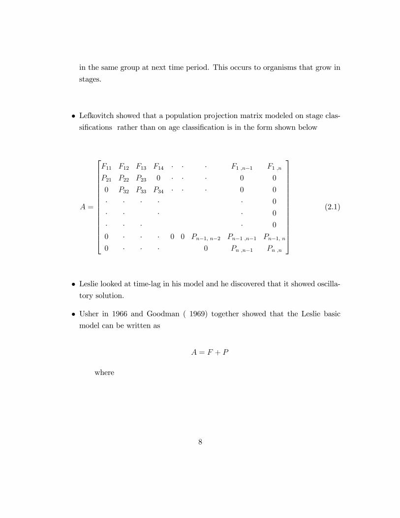
� Lefkovitch showed that a population projection matrix modeled on stage clas-si�cations rather than on age classi�cation is in the form shown below
A =
2666666666666664
F11 F12 F13 F14 � � � F1 ,n�1 F1 ,n
P21 P22 P23 0 � � � 0 0
0 P32 P33 P34 � � � 0 0
� � � � � 0
� � � � 0
� � � � 0
0 � � � 0 0 Pn�1; n�2 Pn�1 ,n�1 Pn�1; n
0 � � � 0 Pn ,n�1 Pn ,n
3777777777777775(2.1)
� Leslie looked at time-lag in his model and he discovered that it showed oscilla-tory solution.
� Usher in 1966 and Goodman ( 1969) together showed that the Leslie basicmodel can be written as
A = F + P
where
8
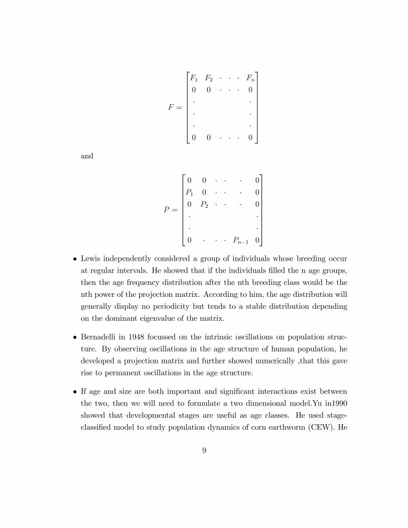
F =
26666666664
F1 F2 � � � Fn0 0 � � � 0
� �� �� �0 0 � � � 0
37777777775and
P =
26666666664
0 0 � � � 0
P1 0 � � � 0
0 P2 � � � 0
� �� �0 � � � Pn�1 0
37777777775� Lewis independently considered a group of individuals whose breeding occurat regular intervals. He showed that if the individuals �lled the n age groups,
then the age frequency distribution after the nth breeding class would be the
nth power of the projection matrix. According to him, the age distribution will
generally display no periodicity but tends to a stable distribution depending
on the dominant eigenvalue of the matrix.
� Bernadelli in 1948 focussed on the intrinsic oscillations on population struc-ture. By observing oscillations in the age structure of human population, he
developed a projection matrix and further showed numerically ,that this gave
rise to permanent oscillations in the age structure.
� If age and size are both important and signi�cant interactions exist betweenthe two, then we will need to formulate a two dimensional model.Yu in1990
showed that developmental stages are useful as age classes. He used stage-
classi�ed model to study population dynamics of corn earthworm (CEW). He
9
divided the CEW into �ve stages and split the �rst stage into four age groups,
the second, third and fourth stages into six age groups, while the last stage he
considered as a single group. His projection matrix was of order 23.
� For large mammals and birds, we only consider age classi�cation and thereforeend up with the Leslie matrix model.
� Wen-Ching Li (1994) applied Leslie matrix model to wild turkey populations.He considered three classes,namely: poults,yearlings and adults. He ended up
with a matrix of order three. Only yearlings and adults are productive.
� G. C Smith and R.C Trout used Leslie matrices to determine wild rabbit popu-lation growth and the potential for control. To examine the rate of population
growth under various control policies, two age categories of rabbits were de-
�ned:young and old categories. A survival rate of 0.95 for young rabbits and
0.05 for old rabbits was used. It was found out that as the maximum age
of young rabbits increased, the variation of the rate of growth with timing of
the control increased. Also, overall � is greatest between late April to early
september and � is least between the periods November to January.
� Neon and Sauer studied population models for passerine birds. They recom-mended an after birth-pulse censuring for population of passerine birds because
the rates of population change for these birds are highly sensitive to fecundity
and/or �rst year survival rate.
10
Chapter 3
Development of Leslie model
The Model is a powerful tool (named after P.H Leslie) and is used to determine the
growth of a population as well as the age distribution within a population.To be able
to develop this model, we make use of the following assumptions:
� We consider only the females in the population
� The maximum age attained by any individual is n years
� The population is grouped into age classes
� An individual chance of surviving from one age class to the next is a function
of its age.
� The survival rate Pi of each age group is known
� The reproduction rate Fi for each age group is known
� The initial age distribution is known
We will put a superscript on the upper right of quantities to signify the point in
time to which the symbol refers and a subscript on the lower right of the quantity
to signify the name of the age class.
11
De�ne
x(k)i =the number of females alive in the group i at time tkPi=the probability that a female of group i at time tk will be alive in group i+1
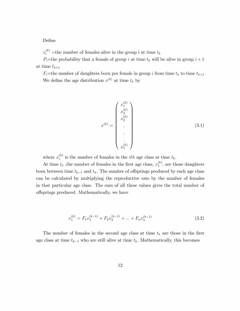
at time tk+1Fi=the number of daughters born per female in group i from time tk to time tk+1We de�ne the age distribution x(k) at time tk by
x(k) =
0BBBBBBBBBBB@
x(k)1
x(k)2
x(k)3
:
:
:
x(k)n
1CCCCCCCCCCCA(3.1)
where x(k)i is the number of females in the ith age class at time tk.
At time tk ,the number of females in the �rst age class, x(k)1 ; are those daughters
born between time tk�1 and tk. The number of o¤springs produced by each age class
can be calculated by multiplying the reproductive rate by the number of females
in that particular age class. The sum of all these values gives the total number of
o¤springs produced. Mathematically, we have
x(k)1 = F1x
(k�1)1 + F2x
(k�1)2 + :::+ Fnx
(k�1)n (3.2)
The number of females in the second age class at time tk are those in the �rst
age class at time tk�1 who are still alive at time tk: Mathematically, this becomes
12
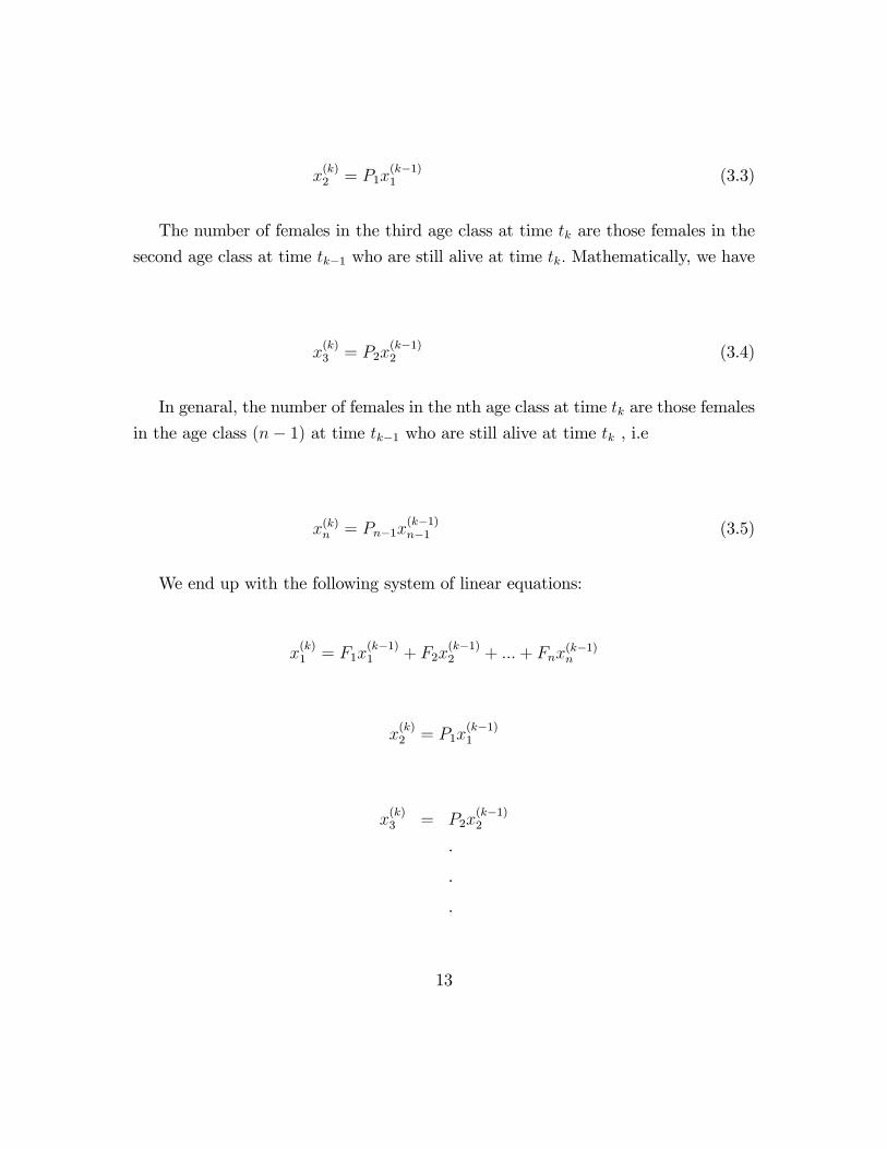
x(k)2 = P1x
(k�1)1 (3.3)
The number of females in the third age class at time tk are those females in the
second age class at time tk�1 who are still alive at time tk: Mathematically, we have
x(k)3 = P2x
(k�1)2 (3.4)
In genaral, the number of females in the nth age class at time tk are those females
in the age class (n� 1) at time tk�1 who are still alive at time tk , i.e
x(k)n = Pn�1x(k�1)n�1 (3.5)
We end up with the following system of linear equations:
x(k)1 = F1x
(k�1)1 + F2x
(k�1)2 + :::+ Fnx
(k�1)n
x(k)2 = P1x
(k�1)1
x(k)3 = P2x
(k�1)2
���
13
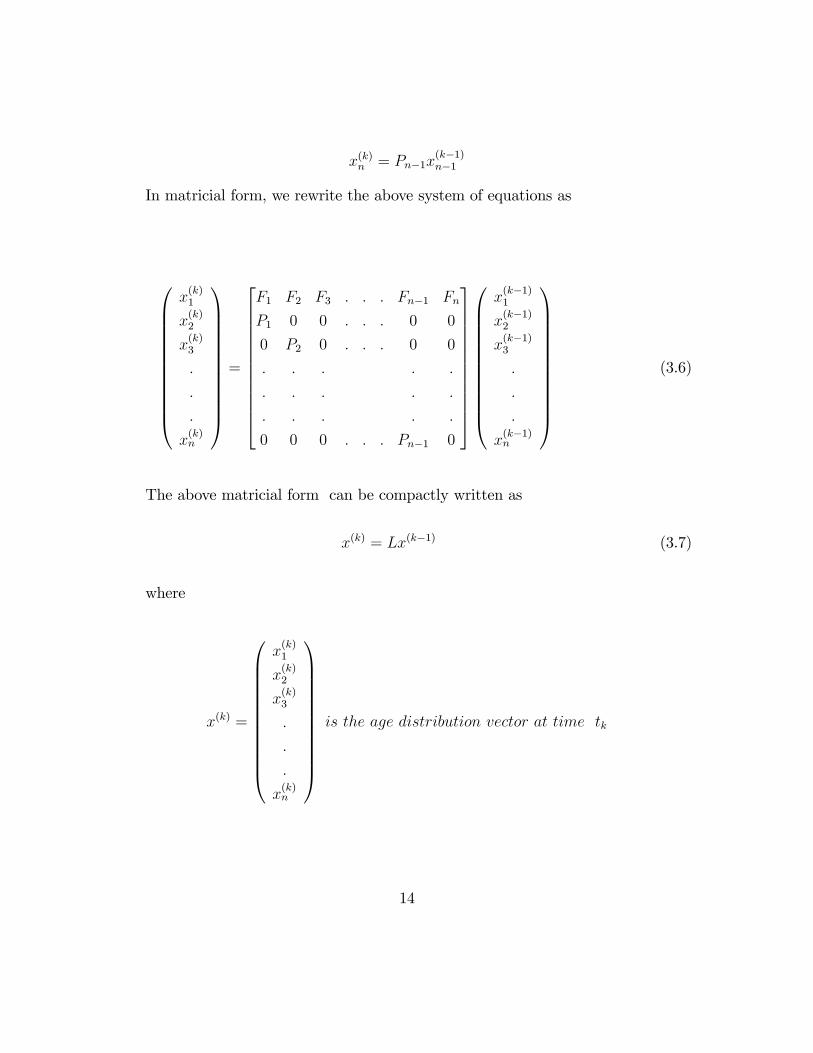
x(k)n = Pn�1x(k�1)n�1
In matricial form, we rewrite the above system of equations as
0BBBBBBBBBBB@
x(k)1
x(k)2
x(k)3
:
:
:
x(k)n
1CCCCCCCCCCCA=
2666666666664
F1 F2 F3 : : : Fn�1 Fn
P1 0 0 : : : 0 0
0 P2 0 : : : 0 0
: : : : :
: : : : :
: : : : :
0 0 0 : : : Pn�1 0
3777777777775
0BBBBBBBBBBB@
x(k�1)1
x(k�1)2
x(k�1)3
:
:
:
x(k�1)n
1CCCCCCCCCCCA(3.6)
The above matricial form can be compactly written as
x(k) = Lx(k�1) (3.7)
where
x(k) =
0BBBBBBBBBBB@
x(k)1
x(k)2
x(k)3
:
:
:
x(k)n
1CCCCCCCCCCCAis the age distribution vector at time tk
14
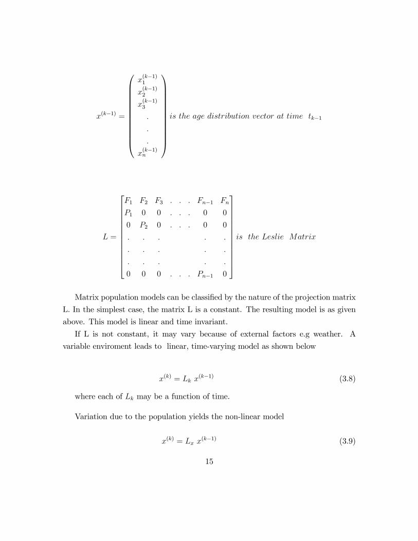
x(k�1) =
0BBBBBBBBBBB@
x(k�1)1
x(k�1)2
x(k�1)3
:
:
:
x(k�1)n
1CCCCCCCCCCCAis the age distribution vector at time tk�1
L =
2666666666664
F1 F2 F3 : : : Fn�1 Fn
P1 0 0 : : : 0 0
0 P2 0 : : : 0 0
: : : : :
: : : : :
: : : : :
0 0 0 : : : Pn�1 0
3777777777775is the Leslie Matrix
Matrix population models can be classi�ed by the nature of the projection matrix
L. In the simplest case, the matrix L is a constant. The resulting model is as given
above. This model is linear and time invariant.
If L is not constant, it may vary because of external factors e.g weather. A
variable enviroment leads to linear, time-varying model as shown below
x(k) = Lk x(k�1) (3.8)
where each of Lk may be a function of time.
Variation due to the population yields the non-linear model
x(k) = Lx x(k�1) (3.9)
15
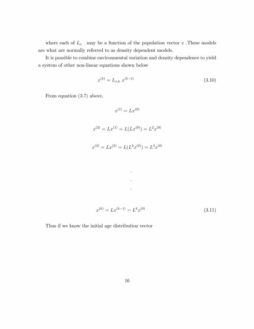
where each of Lx may be a function of the population vector x .These models
are what are normally referred to as density dependent models.
It is possible to combine environmental variation and density dependence to yield
a system of other non-linear equations shown below
x(k) = Lx;k x(k�1) (3.10)
From equation (3:7) above,
x(1) = Lx(0)
x(2) = Lx(1) = L(Lx(0)) = L2x(0)
x(3) = Lx(2) = L(L2x(0)) = L3x(0)
���
x(k) = Lx(k�1) = Lkx(0) (3.11)
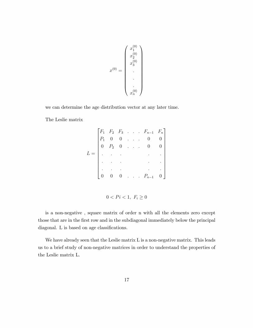
Thus if we know the initial age distribution vector
16
x(0) =
0BBBBBBBBBBB@
x(0)1
x(0)2
x(0)3
:
:
:
x(0)n
1CCCCCCCCCCCAwe can determine the age distribution vector at any later time.
The Leslie matrix
L =
2666666666664
F1 F2 F3 : : : Fn�1 Fn
P1 0 0 : : : 0 0
0 P2 0 : : : 0 0
: : : : :
: : : : :
: : : : :
0 0 0 : : : Pn�1 0
3777777777775
0 < Pi < 1; Fi � 0
is a non-negative , square matrix of order n with all the elements zero except
those that are in the �rst row and in the subdiagonal immediately below the principal
diagonal. L is based on age classi�cations.
We have already seen that the Leslie matrix L is a non-negative matrix. This leads
us to a brief study of non-negative matrices in order to understand the properties of
the Leslie matrix L.
17
Chapter 4
Nonnegative matrices and PerronFrobenius theorem
A 2 Rm�n is said to be a non-negative matrix whenever aij � 0 and this is denotedby writing A � 0 . In general A � B means that aij � bij where aij is an elementin A and bij is an element in B: Similarly, A is a positive matrix when each aij > 0
and is denoted by writing A > 0: More generally, A > B means that each aij > bijSince non-negative matrices have numerous applications, it is natural to inves-
tigate their properties and we do so in this chapter. A primary issue concerns the
extent to which the properties A > 0 or A � 0 translate to spectral properties e.g.to what extent does A have positive ( or non-negative) eigenvalues and eigenvectors.
Here we will focus on matrices An�n and investigate the extent to which this
property (non-negativity) is inherited by the eigenvalues and eigenvectors of A.
First we notice that
A > 0 =) �(A) > 0 where �(A) is the spectral radius of A
18
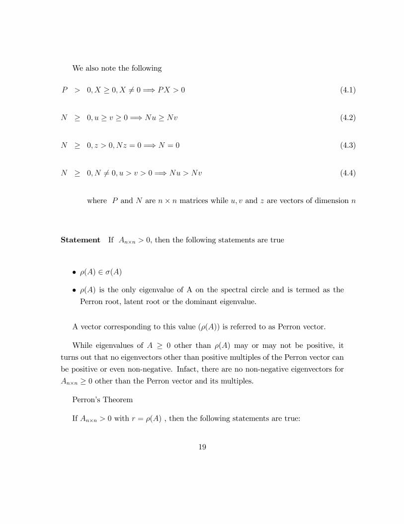
We also note the following
P > 0; X � 0; X 6= 0 =) PX > 0 (4.1)
N � 0; u � v � 0 =) Nu � Nv (4.2)
N � 0; z > 0; Nz = 0 =) N = 0 (4.3)
N � 0; N 6= 0; u > v > 0 =) Nu > Nv (4.4)
where P and N are n� n matrices while u; v and z are vectors of dimension n
Statement If An�n > 0, then the following statements are true
� �(A) 2 �(A)
� �(A) is the only eigenvalue of A on the spectral circle and is termed as the
Perron root, latent root or the dominant eigenvalue.
A vector corresponding to this value (�(A)) is referred to as Perron vector.
While eigenvalues of A � 0 other than �(A) may or may not be positive, it
turns out that no eigenvectors other than positive multiples of the Perron vector can
be positive or even non-negative. Infact, there are no non-negative eigenvectors for
An�n � 0 other than the Perron vector and its multiples.
Perron�s Theorem
If An�n > 0 with r = �(A) , then the following statements are true:
19
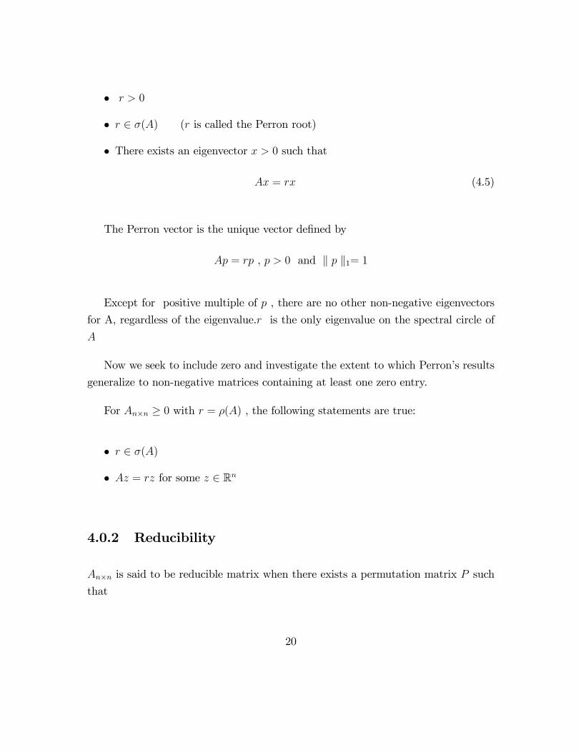
� r > 0
� r 2 �(A) (r is called the Perron root)
� There exists an eigenvector x > 0 such that
Ax = rx (4.5)
The Perron vector is the unique vector de�ned by
Ap = rp , p > 0 and k p k1= 1
Except for positive multiple of p , there are no other non-negative eigenvectors
for A, regardless of the eigenvalue.r is the only eigenvalue on the spectral circle of
A
Now we seek to include zero and investigate the extent to which Perron�s results
generalize to non-negative matrices containing at least one zero entry.
For An�n � 0 with r = �(A) , the following statements are true:
� r 2 �(A)
� Az = rz for some z 2 Rn
4.0.2 Reducibility
An�n is said to be reducible matrix when there exists a permutation matrix P such
that
20

P TAP=
"X Y
0 Z
#
where X and Z are both square.
Otherwise, A is said to be an irreducible matrix
A reducible matrix can always be arranged by numbering the stages , into normal
form: "B O
C D
#(4.6)
where the square submatrices B and D are either irreducible or can themselves
be divided to eventually yield a series of irreducible diagonal blocks (Gantmacher
1959).
An irreducible matrix always has a real positive latent root �1 that is distinct.
The absolute values of all other roots are less than or equal to �1 and in practice the
other roots are either complex or else negative.
Corresponding to �1 is an eigenvector whose entries are non-negative. No other
eigenvector of non-negative elements exists, disregarding multiples of the eigenvector.
4.0.3 Primitive Matrices
Let A � 0 be an irreducible matrix and let the dominant eigenvalue be �� . Supposethere are exactly h eigenvalues of modulus ��, say
21
�� = �1
then
�1 = j �2 j= ::: =j �h j
If h = 1,the matrix A is called primitive , that is, a non-negative irreducible
matrix A having only one eigenvalue , r = �(A) , on its spectral circle is said to be
a primitive matrix.
If h > 1 , the matrix A is called imprimitive and h is called the index of imprim-
itivity.
We next state without proof a su¢ cient condition for primitivity.
Corollary 7 If a non-negative irreducible matrix A has at least one positive diagonalelement, then A is primitive.
Below is a statement to show how powers of a non-negative matrix determine
whether or not the matrix is primitive
Lemma 8 Frobenius test for Primitivity
A � 0 is primitive i¤ Am > 0 for some m > 0
This is to say that an irreducible non-negative matrix A is primitive if it becomes
positive when raised to su¢ ciently high powers. A reducible matrix cannot be prim-
itive because when the matrix (4:6) above is raised to powers , the upper-right block
remains zero.
22
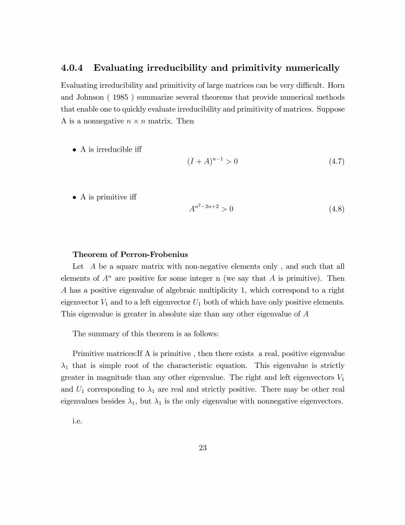
4.0.4 Evaluating irreducibility and primitivity numerically
Evaluating irreducibility and primitivity of large matrices can be very di¢ cult. Horn
and Johnson ( 1985 ) summarize several theorems that provide numerical methods
that enable one to quickly evaluate irreducibility and primitivity of matrices. Suppose
A is a nonnegative n� n matrix. Then
� A is irreducible i¤(I + A)n�1 > 0 (4.7)
� A is primitive i¤An
2�2n+2 > 0 (4.8)
Theorem of Perron-FrobeniusLet A be a square matrix with non-negative elements only , and such that all
elements of An are positive for some integer n (we say that A is primitive). Then
A has a positive eigenvalue of algebraic multiplicity 1, which correspond to a right
eigenvector V1 and to a left eigenvector U1 both of which have only positive elements.
This eigenvalue is greater in absolute size than any other eigenvalue of A
The summary of this theorem is as follows:
Primitive matrices:If A is primitive , then there exists a real, positive eigenvalue
�1 that is simple root of the characteristic equation. This eigenvalue is strictly
greater in magnitude than any other eigenvalue. The right and left eigenvectors V1and U1 corresponding to �1 are real and strictly positive. There may be other real
eigenvalues besides �1, but �1 is the only eigenvalue with nonnegative eigenvectors.
i.e.
23
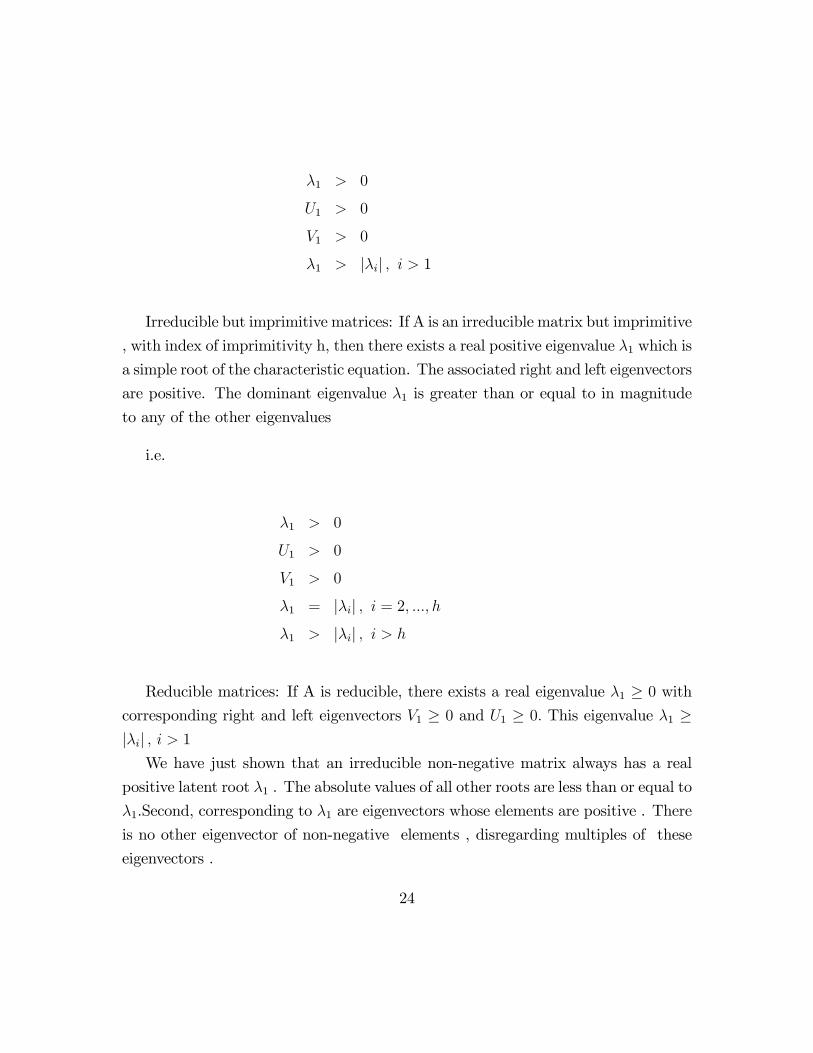
�1 > 0
U1 > 0
V1 > 0
�1 > j�ij ; i > 1
Irreducible but imprimitive matrices: If A is an irreducible matrix but imprimitive
, with index of imprimitivity h, then there exists a real positive eigenvalue �1 which is
a simple root of the characteristic equation. The associated right and left eigenvectors
are positive. The dominant eigenvalue �1 is greater than or equal to in magnitude
to any of the other eigenvalues
i.e.
�1 > 0
U1 > 0
V1 > 0
�1 = j�ij ; i = 2; :::; h�1 > j�ij ; i > h
Reducible matrices: If A is reducible, there exists a real eigenvalue �1 � 0 withcorresponding right and left eigenvectors V1 � 0 and U1 � 0: This eigenvalue �1 �j�ij ; i > 1We have just shown that an irreducible non-negative matrix always has a real
positive latent root �1 . The absolute values of all other roots are less than or equal to
�1.Second, corresponding to �1 are eigenvectors whose elements are positive . There
is no other eigenvector of non-negative elements , disregarding multiples of these
eigenvectors .
24
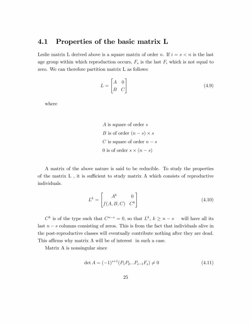
4.1 Properties of the basic matrix L
Leslie matrix L derived above is a square matrix of order n. If i = s < n is the last
age group within which reproduction occurs, Fs is the last Fi which is not equal to
zero. We can therefore partition matrix L as follows:
L =
"A 0
B C
#(4.9)
where
A is square of order s
B is of order (n� s)� sC is square of order n� s0 is of order s� (n� s)
A matrix of the above nature is said to be reducible. To study the properties
of the matrix L , it is su¢ cient to study matrix A which consists of reproductive
individuals.
Lk =
"Ak 0
f(A;B;C) Ck
#(4.10)
Ck is of the type such that Cn�s = 0; so that Lk, k � n � s will have all its
last n� s columns consisting of zeros. This is from the fact that individuals alive in
the post-reproductive classes will eventually contribute nothing after they are dead.
This a¢ rms why matrix A will be of interest in such a case.
Matrix A is nonsingular since
detA = (�1)s+1(P1P2:::Ps�1Fs) 6= 0 (4.11)
25
If the entire population is productive, then matrix A will be the entire matrix
and we say in this case that A = L is irreducible.
We will later show that the Leslie matrix L used in elephants demography falls in
a restricted subclass of irreducible non-negative matrices called primitive matrices.
From the Perron- Frobenius theory, L has a unique root �1 which is larger in
magnitude than any other root (eigenvalue) of L. Corresponding to �1 is a eigenvector
which is positive and no other non-negative eigenvector will exist for matrix L.
4.1.1 Parameter estimation
Survival probability Pi
The values of Pi is usually obtained from a life table or experiments. It is usually
assumed that ( Leslie 1945,Caughley 1977:87)
Pi =li+1li
(4.12)
Pi is assumed to be constant over a unit of time.
Fecundity rates Fi
Fi is determined not only by the average number of female births per mother per
time period , mi in the life table , but also including infant survival rates (Leslie
1945). We divide populations into two breeding systems: birth-�ow and birth-purse
populations.
Birth-�ow breeding Here reproduction is continuous. Estimation of Fi involves
integration of fertility and infant mortality functions over the continuous time inter-
val.
26
Birth-pulse breeding Populations in this system reproduce during a short period
of time per year. In this system , it is important to know the exact breeding period
with respect to the time step . Estimation of Fi will be in�uenced by way of census.
Census before reproduction or after reproduction give rise to di¤erent value of Fi:
Since births occur during the next birthday of an individual, the probability of
surviving for a fraction 1� p is P 1�pi . For the individual to be counted in n1(t+ 1);
it must survive a fraction p of a time unit , and that probability is determined by
l(p):
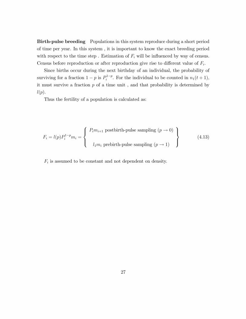
Thus the fertility of a population is calculated as:
Fi = l(p)P1�pi mi =
8><>:Pimi+1 postbirth-pulse sampling (p! 0)
l1mi prebirth-pulse sampling (p! 1)
9>=>; (4.13)
Fi is assumed to be constant and not dependent on density.
27
Chapter 5
Eigensystem
5.1 Eigenvalues and corresponding eigenvectors
Consider the system
x(k) = Lx(k�1)
We apply linear algebra techniques to the above model to interpret several bio-
logical phenomena.
If L has the formula
LVi = �iVi (5.1)
then �i ; i = 1; 2; :::; n are the eigenvalues of L. For the above system
j�1j > j�2j � j�3j � � � � � j�nj
Vi are the corresponding linearly independent eigenvectors.
The eigenvalues are arrived at by solving the system
28
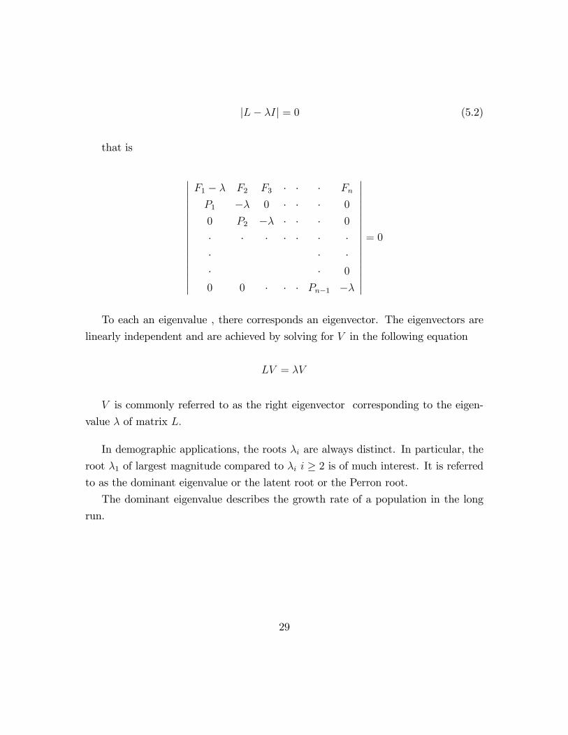
jL� �Ij = 0 (5.2)
that is
�����������������
F1 � � F2 F3 � � � Fn
P1 �� 0 � � � 0
0 P2 �� � � � 0
� � � � � � �� � �� � 0
0 0 � � � Pn�1 ��
�����������������= 0
To each an eigenvalue , there corresponds an eigenvector. The eigenvectors are
linearly independent and are achieved by solving for V in the following equation
LV = �V
V is commonly referred to as the right eigenvector corresponding to the eigen-
value � of matrix L:
In demographic applications, the roots �i are always distinct. In particular, the
root �1 of largest magnitude compared to �i i � 2 is of much interest. It is referredto as the dominant eigenvalue or the latent root or the Perron root.
The dominant eigenvalue describes the growth rate of a population in the long
run.
29
�1 = 1; the population is stationary
�1 > 1; over population will be experienced.
�1 < 1; the population diminishes.
For �1 > 1, one may think of harvesting as an option in order to keep the
population stable.
For the system
x(k) = Ax(k�1) (5:1:3)
where A is an arbitrary matrix,
The system (5:1:3) is said to be asymptotically stable i¤ the eigenvalues of A
have magnitude less than 1, that is, j�ij < 1 for every i . The vector x(k) will tend toan equilibrium point for any initial condition if the system is asymptotically stable.
Once the system state vector is equal to an equilibrium point, it will remain equal
to it for all time in the future.
The system (5:1:3) is said to be marginally stable if the magnitude of the eigen-
values are less or equal to 1. If 1 is an eigenvalue of A, then the corresponding
eigenvector is an equilibrium point. If 1 is not an eigenvalue of A , the origin is the
only equilibrium of the system.
Each eigenvalue de�nes a characteristic growth as well as a characteristic fre-
quency of oscillation. For a discrete-time system, we do not have oscillations if
the eigenvalues are positive. Oscillations are only derived from negative or complex
eigenvalues.
30
5.2 Vertical Stable Vectors
From the Perron-Frobenius theorem, the Leslie matrix which is non-negative, has
a positive dominant eigenvalue which is simple. Thus a population based on Leslie
matrix will in the long run have a growth factor. That is , from some year on, next
year�s population will be a multiple of this year�s. Therefore, after some time, the
population in the age-classes will grow proportionally. The proportions of popula-
tions in the age classes will be constant. This age composition is called a stable-age
distribution.
Mathematically, we have
x(k+1) = �1x(k) (5.3)
where the factor �1 is the dominant eigenvalue of the Leslie matrix L. If V1 is
the associated right eigenvector,we can obtain the stable-age distribution from V1:
Let
V1 =
2666666666664
v1
v2
v3
���vn
3777777777775and
C = v1 + v2 + � � �+ vn
Then the stable-age distribution ,S1, is expressed as
31
S1 =
2666666666664
v1Cv2Cv3C
���vnC
3777777777775(5.4)
The sum of the elements of S is unity.
The right eigenvectors are linearly independent. This means that there exists no
nonzero constant bi such that
b1V1 + b2V2 + :::+ bnVn = 0
If the right eigenvectors Vi ; i = 1; 2; :::; n are arranged side by side to constitute
a matrix V below
V = [V1 V2 � � � Vn] =
26666666664
a11 a12 � � � a1n
a21 a22 � � � a21
� �� �� �an1 a2n � � � ann
37777777775(5.5)
then using the fact that the columns of the matrix V are Vi and that
LVi = �iVi
we have
LV = V � (5.6)
32
where � is the diagonal matrix
� =
26666666664
�1 0 � � � 0
0 �2 �� �� �� 0
0 � � � 0 �n
37777777775(5.7)
that is
26666666664
F1 F2 : : Fn�1 Fn
P1 0 : : 0 0
0 P2 : : 0 0
: : : :
: : : :
0 0 : : Pn�1 0
37777777775
26666666664
a11 a12 � � a1;n
a21 a22 � � a2;n
� �� �� �an;1 a2;n � � an;n
37777777775=
26666666664
a11 a12 � � a1;n
a21 a22 � � a2;n
� �� �� �an;1 an;2 � � an;n
37777777775
26666666664
�1 0 � � � 0
0 �2 �� �� �� 0
0 � � � 0 �n
37777777775
From
LV = V �
we have
L = V �V �1 (5.8)
thus
33
L2 =�V �V �1
� �V �V �1
�= V �
�V �1V
��V �1
= V �2V �1
Repeating the multiplication gives
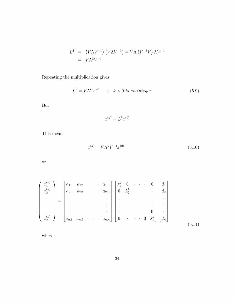
Lk = V �kV �1 ; k > 0 is an integer (5.9)
But
x(k) = Lkx(0)
This means
x(k) = V �kV �1x(0) (5.10)
or
0BBBBBBBBB@
x(k)1
x(k)2
:
:
:
x(k)n
1CCCCCCCCCA=
26666666664
a11 a12 � � � a1;n
a21 a22 � � � a2;n
� �� �� �an;1 an;2 � � � an;n
37777777775
26666666664
�k1 0 � � � 0
0 �k2 �� �� �� 0
0 � � � 0 �kn
37777777775
26666666664
d1
d2
���dn
37777777775(5.11)
where
34
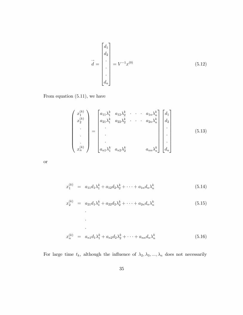
!d =
26666666664
d1
d2
���dn
37777777775= V �1x(0) (5.12)
From equation (5:11), we have
0BBBBBBBBB@
x(k)1
x(k)2
:
:
:
x(k)n
1CCCCCCCCCA=
26666666664
a11�k1 a12�
k2 � � � a1n�
kn
a21�k1 a22�
k2 � � � a2n�
kn
���
an1�k1 an2�
k2 ann�
kn
37777777775
26666666664
d1
d2
���dn
37777777775(5.13)
or
x(k)1 = a11d1�
k1 + a12d2�
k2 + � � �+ a1ndn�kn (5.14)
x(k)2 = a21d1�
k1 + a22d2�
k2 + � � �+ a2ndn�kn (5.15)
���
x(k)n = an1d1�k1 + an2d2�
k2 + � � �+ anndn�kn (5.16)
For large time tk, although the in�uence of �2; �3; :::; �n does not necessarily
35
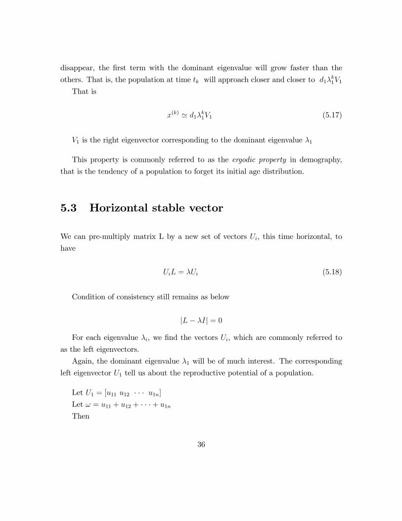
disappear, the �rst term with the dominant eigenvalue will grow faster than the
others. That is, the population at time tk will approach closer and closer to d1�k1V1
That is
x(k) ' d1�k1V1 (5.17)
V1 is the right eigenvector corresponding to the dominant eigenvalue �1
This property is commonly referred to as the ergodic property in demography,
that is the tendency of a population to forget its initial age distribution.
5.3 Horizontal stable vector
We can pre-multiply matrix L by a new set of vectors Ui, this time horizontal, to
have
UiL = �Ui (5.18)
Condition of consistency still remains as below
jL� �Ij = 0
For each eigenvalue �i, we �nd the vectors Ui, which are commonly referred to
as the left eigenvectors.
Again, the dominant eigenvalue �1 will be of much interest. The corresponding
left eigenvector U1 tell us about the reproductive potential of a population.
Let U1 = [u11 u12 � � � u1n]Let ! = u11 + u12 + � � �+ u1nThen
36
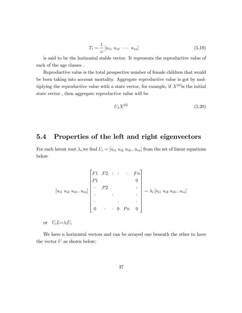
T1 =1
![u11 u12 � � � u1n] (5.19)
is said to be the horizontal stable vector. It represents the reproductive value of
each of the age classes .
Reproductive value is the total prospective number of female children that would
be born taking into account mortality. Aggregate reproductive value is got by mul-
tiplying the reproductive value with a state vector, for example, if X(0)is the initial
state vector , then aggregate reproductive value will be
U1X(0) (5.20)
5.4 Properties of the left and right eigenvectors
For each latent root �i,we �nd Ui = [ui1 ui2 ui3:::uin] from the set of linear equations
below
[ui1 ui2 ui3:::uin]
26666666664
F1 F2 � � � Fn
P1 0
� P2 �� � �� � �0 � � 0 Pn 0
37777777775= �i [ui1 ui2 ui3:::uin]
or UiL=�iUi
We have n horizontal vectors and can be arrayed one beneath the other to have
the vector U as shown below;
37
U =
2666666666664
U1
U2
���
Un�1
Un
3777777777775(5.21)
where each Ui is a row vector
The stable vectors posses an orthogonality property by which if i 6= j , then
UiVj = 0 (5.22)
where
LVj = �jVj (5.23)
(5:4:2) is from the fact that if we premultiply (5:4:3) by Ui, we get
UiLVj = Ui�jVj
= �jUiVj (5.24)
It is also true to have
UiL = �iUi (5.25)
Multiplying (4) on the right by Vj, we get
38
UiLVj = �iUiVj (5.26)
Now (5:4:4) and (5:4:6) gives
0 = (�j � �i)UiVj , �j 6= �i
which gives
UiVj = 0 for i 6= j
In demography, the vector U1 corresponding to the dominant eigenvalue �1 is the
one of much interest. It represents the left eigenvector corresponding to the dominant
eigenvalue and tells us about the reproductive potential of a population.
The equation above can be rewritten as
UL = �U
where � is a diagonal matrix of order n whose diagonal elements are the various
eigenvalues of matrix L
The above equation can also be written as
L = U�1�U (5.27)
We also noted earlier that if V is the matrix of right eigenvectors, then
L = V �V �1
so that
U�1�U = V �V �1 (5.28)
Now normalising Ui by the dividing it with UiVi , we have
39
U i =UiUiVi
(5:4:9) (5.29)
This gives
U iVj = 1 for i = j (5.30)
= 0 for i 6= j
The above helps us express an observed age distribution, say the state vector X(0)
as a sum of the stable vectors each multiplied by a constant, that is,
X(0) = c1V1 + c2V2 + :::+ cnVn (5.31)
To �nd ci, premultiply (5:31) by the normalised U i and have
U iX(0) = c1U iV1 = c2U iV2 + :::+ cnU iVn (5.32)
This gives
U iX(0) = ci
or
ci =UiX
(0)
UiVi(5.33)
Premultiplying (5:31) by L gives;
LX(0) = c1LV1 + c2LV2 + :::+ cnLVn
= �1c1V1 + �2c2V2 + :::+ �ncnVn (5.34)
40
This shows that after k steps, the population will be
LkX(0) = �k1c1V1 + �k2c2V2 + :::+ �
kncnVn (5.35)
After a long time has passed, only the �rst term in (5:35) counts and we write
X(k) = LkX(0) = �k1c1V1 (5.36)
c1 =U1X
(0)
U1V1is termed as the stable equivalent population (5.37)
5.4.1 E¤ects of eigenvalues
The long term behavior of a population depends on the eigenvalues �i as they are
raised to high powers.
� If �i > 1 , �ki produces exponential growth� If � < 1 , we have exponential decay� If �1 < �i < 0; then �ki exhibits damped oscillations.
� If �i < �1 ,then �ki produces diverging oscillations.� Complex eigenvalues produce oscillations.
If � = a+ bi = j�j (cos �+ i sin �) , complex conjugate is � = a� bi: Thus raising� to k th power yields
�k = j�jk (cos �k + i sin �k)
The solution to the projection equation will thus contain terms of the form
41
�k + �k= j�jk 2 cos �k (5.38)
Thus ,as a complex eigenvalue raised to higher and higher powers , its magnitude
j�jk increases /decreases exponentially , depending on whether j�j is greater or lessthan 1.
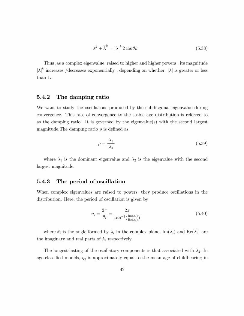
5.4.2 The damping ratio
We want to study the oscillations produced by the subdiagonal eigenvalue during
convergence. This rate of convergence to the stable age distribution is referred to
as the damping ratio. It is governed by the eigenvalue(s) with the second largest
magnitude.The damping ratio � is de�ned as
� =�1j�2j
(5.39)
where �1 is the dominant eigenvalue and �2 is the eigenvalue with the second
largest magnitude.
5.4.3 The period of oscillation
When complex eigenvalues are raised to powers, they produce oscillations in the
distribution. Here, the period of oscillation is given by
�i =2�
�i=
2�
tan�1( Im(�i)Re(�i)
)(5.40)
where �i is the angle formed by �i in the complex plane, Im(�i) and Re(�i) are
the imaginary and real parts of �i respectively.
The longest-lasting of the oscillatory components is that associated with �2: In
age-classi�ed models, �2 is approximately equal to the mean age of childbearing in
42
the stable population (Lotka 1945, Coale 1972)
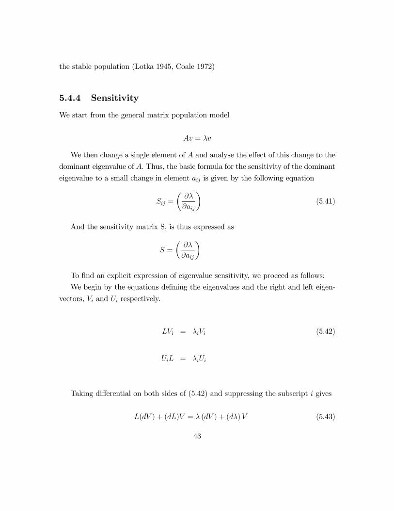
5.4.4 Sensitivity
We start from the general matrix population model
Av = �v
We then change a single element of A and analyse the e¤ect of this change to the
dominant eigenvalue of A: Thus, the basic formula for the sensitivity of the dominant
eigenvalue to a small change in element aij is given by the following equation
Sij =
�@�
@aij
�(5.41)
And the sensitivity matrix S, is thus expressed as
S =
�@�
@aij
�
To �nd an explicit expression of eigenvalue sensitivity, we proceed as follows:
We begin by the equations de�ning the eigenvalues and the right and left eigen-
vectors, Vi and Ui respectively.
LVi = �iVi (5.42)
UiL = �iUi
Taking di¤erential on both sides of (5:42) and suppressing the subscript i gives
L(dV ) + (dL)V = � (dV ) + (d�)V (5.43)
43
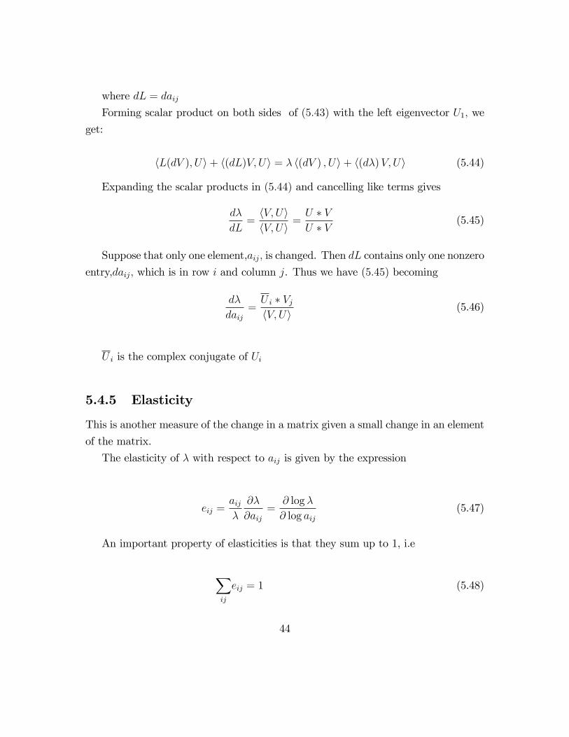
where dL = daijForming scalar product on both sides of (5:43) with the left eigenvector U1; we
get:
hL(dV ); Ui+ h(dL)V; Ui = � h(dV ) ; Ui+ h(d�)V; Ui (5.44)
Expanding the scalar products in (5:44) and cancelling like terms gives
d�
dL=hV; UihV; Ui =
U � VU � V (5.45)
Suppose that only one element,aij; is changed. Then dL contains only one nonzero
entry,daij; which is in row i and column j. Thus we have (5:45) becoming
d�
daij=U i � VjhV; Ui (5.46)
U i is the complex conjugate of Ui
5.4.5 Elasticity
This is another measure of the change in a matrix given a small change in an element
of the matrix.
The elasticity of � with respect to aij is given by the expression
eij =aij�
@�
@aij=@ log �
@ log aij(5.47)
An important property of elasticities is that they sum up to 1, i.e
Xij
eij = 1 (5.48)
44
5.5 Some theorems and proofs for the Leslie Ma-
trix models
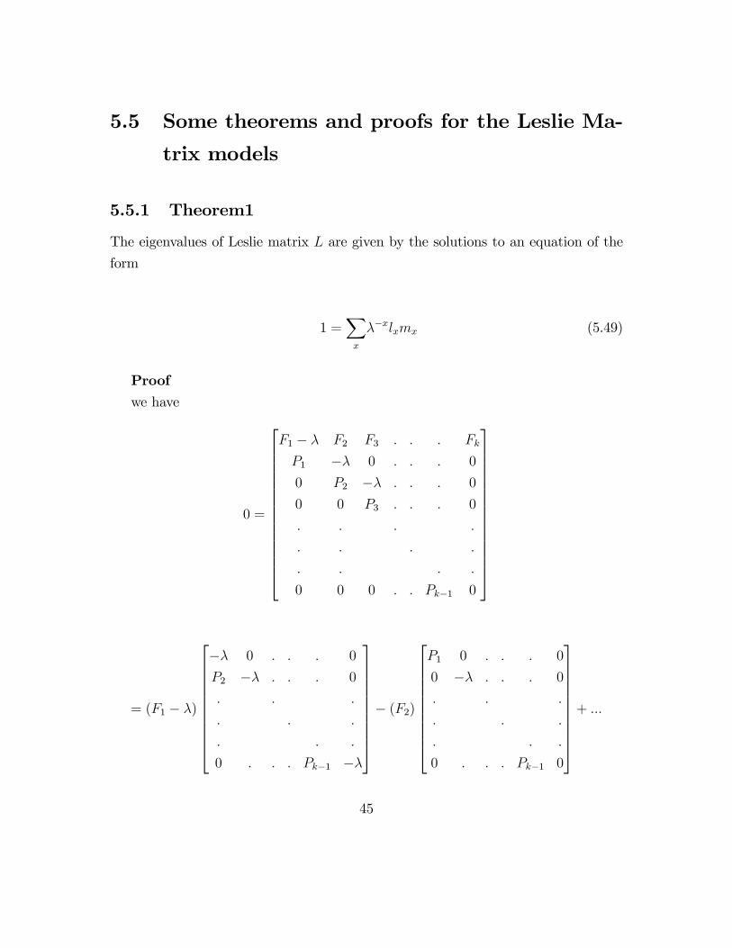
5.5.1 Theorem1
The eigenvalues of Leslie matrix L are given by the solutions to an equation of the
form
1 =Xx
��xlxmx (5.49)
Proofwe have
0 =
2666666666666664
F1 � � F2 F3 : : : Fk
P1 �� 0 : : : 0
0 P2 �� : : : 0
0 0 P3 : : : 0
: : : :
: : : :
: : : :
0 0 0 : : Pk�1 0
3777777777777775
= (F1 � �)
26666666664
�� 0 : : : 0
P2 �� : : : 0
: : :
: : :
: : :
0 : : : Pk�1 ��
37777777775� (F2)
26666666664
P1 0 : : : 0
0 �� : : : 0
: : :
: : :
: : :
0 : : : Pk�1 0
37777777775+ :::
45
= (F1 � �)(��)k�1 + (�1)F2[P1(��)k�2] + :::
= (F1 � �)(�1)k�1�k�1 � F2P1(�1)k�2�k�2 + F3P1P2(�1)k�3�k�3 � :::
= (�1)k�1[F1�k�1 � �k + F2P1�k�2 + F3P1P2�k�3 + :::]
or
F1�k�1 � �k + F2P1�k�2 + F3P1P2�k�3 + ::: = 0
or
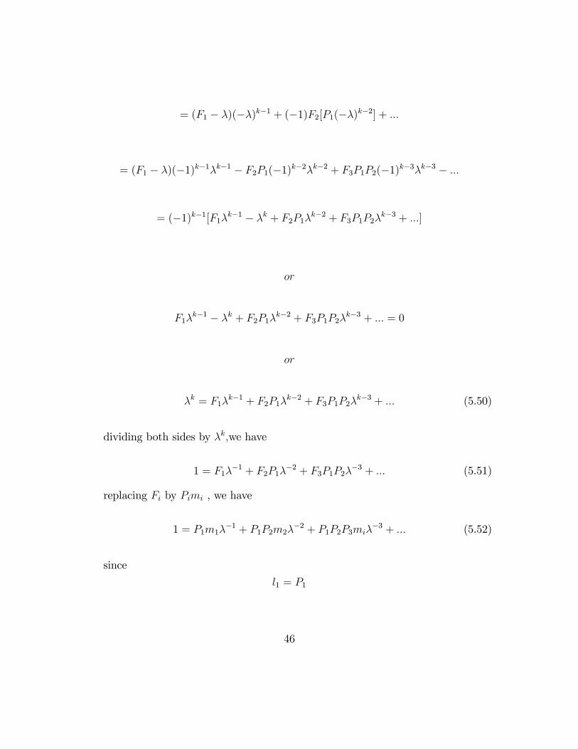
�k = F1�k�1 + F2P1�
k�2 + F3P1P2�k�3 + ::: (5.50)
dividing both sides by �k;we have
1 = F1��1 + F2P1�
�2 + F3P1P2��3 + ::: (5.51)
replacing Fi by Pimi , we have
1 = P1m1��1 + P1P2m2�
�2 + P1P2P3mi��3 + ::: (5.52)
since
l1 = P1
46
l2 = P1P2
l3 = P1P2P3
we have
1 =Xx
��xlxmx
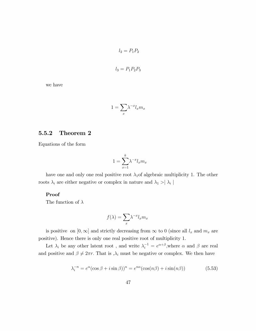
5.5.2 Theorem 2
Equations of the form
1 =kXx=1
��xlxmx
have one and only one real positive root �1of algebraic multiplicity 1. The other
roots �i are either negative or complex in nature and �1 >j �i j
ProofThe function of �
f(�) =Xx
��xlxmx
is positive on [0;1] and strictly decreasing from1 to 0 (since all lx and mx are
positive). Hence there is only one real positive root of multiplicity 1.
Let �i be any other latent root , and write ��1i = e�+�;where � and � are real
and positive and � 6= 2�r: That is ,�i must be negative or complex. We then have
��ni = e�(cos � + i sin �))n = en�(cos(n�) + i sin(n�)) (5.53)
47
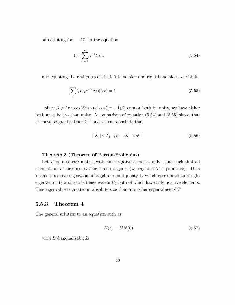
substituting for ��1i in the equation
1 =
kXx=1
��xlxmx (5.54)
and equating the real parts of the left hand side and right hand side, we obtain
Xx
lxmxex� cos(�x) = 1 (5.55)
since � 6= 2�r; cos(�x) and cos((x + 1)�) cannot both be unity, we have eitherboth must be less than unity. A comparison of equation (5:54) and (5:55) shows that
e� must be greater than ��1 and we can conclude that
j �i j< �1 for all i 6= 1 (5.56)
Theorem 3 (Theorem of Perron-Frobenius)Let T be a square matrix with non-negative elements only , and such that all
elements of T n are positive for some integer n (we say that T is primitive). Then
T has a positive eigenvalue of algebraic multiplicity 1, which correspond to a right
eigenvector V1 and to a left eigenvector U1 both of which have only positive elements.
This eigenvalue is greater in absolute size than any other eigenvalues of T
5.5.3 Theorem 4
The general solution to an equation such as
N(t) = LtN(0) (5.57)
with L diagonalizable,is
48
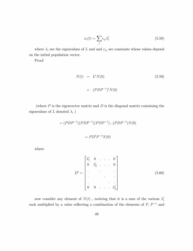
ni(t) =Xj
cij�ti (5.58)
where �i are the eigenvalues of L and and cij are constants whose values depend
on the initial population vector.
Proof
N(t) = LtN(0) (5.59)
= (PDP�1)tN(0)
(where P is the eigenvector matrix and D is the diagonal matrix containing the
eigenvalues of L denoted �i )
= (PDP�1)(PDP�1)(PDP�1):::(PDP�1)N(0)
= PDtP�1N(0)
where
Dt =
26666666664
�t1 0 : : : 0
0 �t2 : : : 0
: : :
: : :
: : :
0 0 : : : �tk
37777777775(5.60)
now consider any element of N(t) , noticing that it is a sum of the various �tieach multiplied by a value re�ecting a combination of the elements of P; P�1 and
49
N(0) ,i.e.
ni(t) =X
Cij�tj
where f�jg are the eigenvalues of L and the Cij are constants whose values dependon the initial population vector.
50
Chapter 6
Application to Amboseli elephants
6.1 Facts about the African elephant
Elephants are the largest living land mammal found in most regions of Africa.They
have massive bodies, broad feet, loose skin with large, thin and �oppy ears which
provide extensive cooling to the body during hot periods. The upper lip and nose are
elongated into a �exible trunk reaching nearly to the ground. This is used for picking
food and drawing water during feeding.The upper incisor teeth are elongated into
tusks valued for ivory. A gland between the eye and the ear often produces a sub-
stance called musth. During these periods, the animal is in an excitable, dangerous
condition called musth period.
Elephants are browsing animals feeding on leaves ,shoots,tall grasses and fruits.
They are relational animals, living and travelling in groups called family units of
between 15 and 30 individual composed of a matriarch (female elder) , her daughters
and their o¤springs. Upto 5 family units associate in bond groups temporarily. Male
older than 13 years are generally solitary or live in small groups.
A single calf is born after a gestation period of 22 months and is nursed for
approximately 5 years . Elephants reach maturity at between 11-20 years of age
with a lifespan of up to 65 years.The African elephant is commonly referred to as
Loxodonta africana and are generally found at the south of the Sahara. Bulls may
51
reach a shoulder height of 13 ft and weigh upto 8 tons. Cows are slightly smaller
with slender tusks.
6.2 Measuring elephant ages
Several equations for measuring elephant ages are available. An example is the
shoulder-height equations deduced by Von Bertalan¤y (1938). The equations relate
shoulder height (h) of elephants ,of di¤erent gender, to their ages (x).The equations
are given below:
male(1� 20years) : h(x) = 265(1� e�0:114(x+3:95))cm (6.1)
male(20� 60years) : h(x) = 307(1� e�0:166(x�10:48))cm (6.2)
female(2� 60years) : h(x) = 252(1� e�0:099(x+6:00))cm (6.3)
If we want to deduce the age from the height, we use the following equations:
male(96� 245cm) : x(h) = � log(1� h
265)
0:114� 3:95years (6.4)
male(245� 307cm) : x(h) = � log(1� h
307)
0:166+ 10:48years (6.5)
female(113� 252cm) : x(h) = � log(1� h
252)
0:099� 6:00years (6.6)
6.2.1
52
6.2.2 Amboseli elephants
The Amboseli elephants are unusual in Africa because they have been relatively
una¤ected by human activities for example settlement, poaching and culling as part
of Park Management Program. This is because of the following:The land surrounding
Amboseli National Park belongs to the Maasai community who have coexisted well
with wildlife. Second, the presence of tourists in and around the National Park makes
it di¢ cult for poachers to operate. Finally, the presence and monitoring of elephants
by researchers has served well in conserving the elephant population.
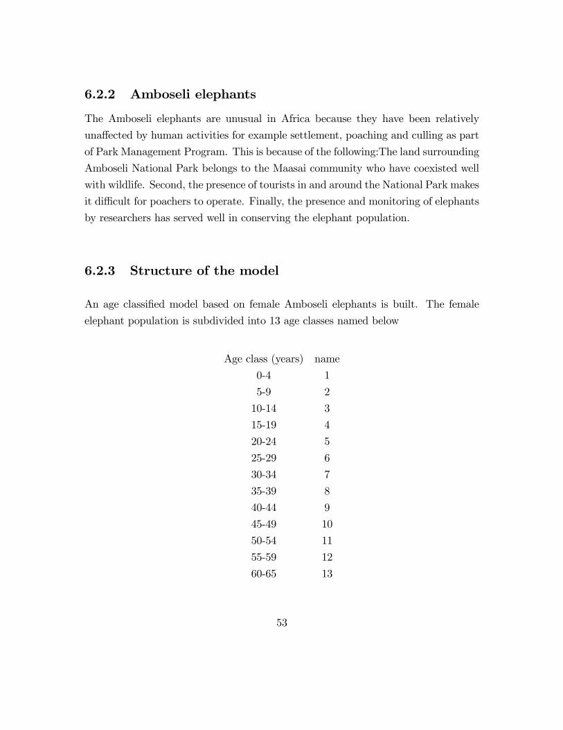
6.2.3 Structure of the model
An age classi�ed model based on female Amboseli elephants is built. The female
elephant population is subdivided into 13 age classes named below
Age class (years) name
0-4 1
5-9 2
10-14 3
15-19 4
20-24 5
25-29 6
30-34 7
35-39 8
40-44 9
45-49 10
50-54 11
55-59 12
60-65 13
53
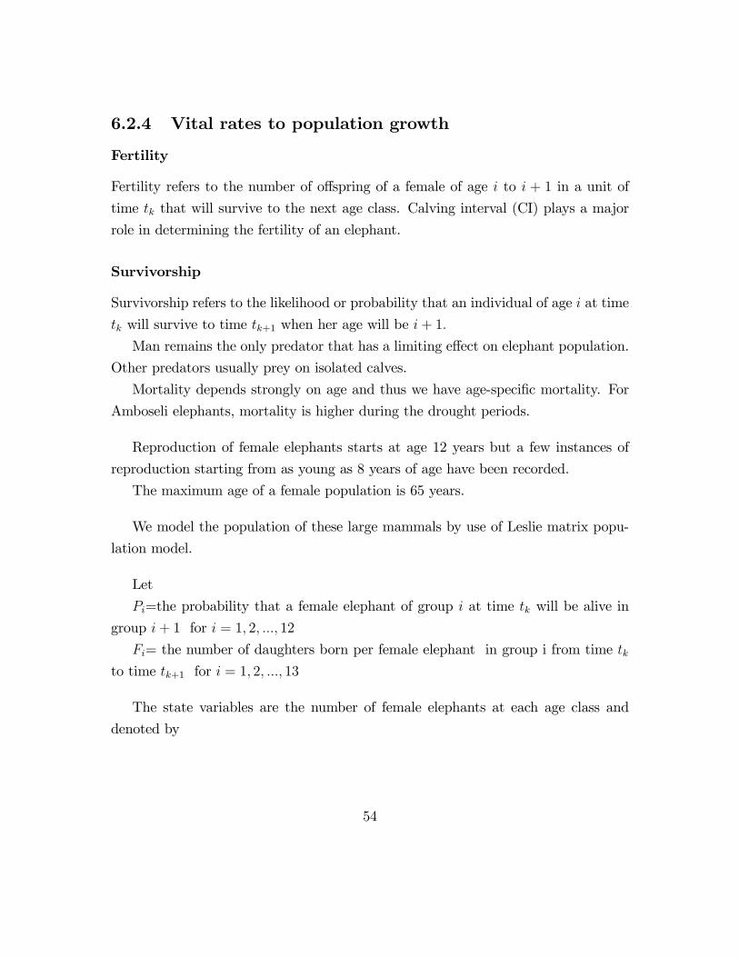
6.2.4 Vital rates to population growth
Fertility
Fertility refers to the number of o¤spring of a female of age i to i + 1 in a unit of
time tk that will survive to the next age class. Calving interval (CI) plays a major
role in determining the fertility of an elephant.
Survivorship
Survivorship refers to the likelihood or probability that an individual of age i at time
tk will survive to time tk+1 when her age will be i+ 1:
Man remains the only predator that has a limiting e¤ect on elephant population.
Other predators usually prey on isolated calves.
Mortality depends strongly on age and thus we have age-speci�c mortality. For
Amboseli elephants, mortality is higher during the drought periods.
Reproduction of female elephants starts at age 12 years but a few instances of
reproduction starting from as young as 8 years of age have been recorded.
The maximum age of a female population is 65 years.
We model the population of these large mammals by use of Leslie matrix popu-
lation model.
Let
Pi=the probability that a female elephant of group i at time tk will be alive in
group i+ 1 for i = 1; 2; :::; 12
Fi= the number of daughters born per female elephant in group i from time tkto time tk+1 for i = 1; 2; :::; 13
The state variables are the number of female elephants at each age class and
denoted by
54
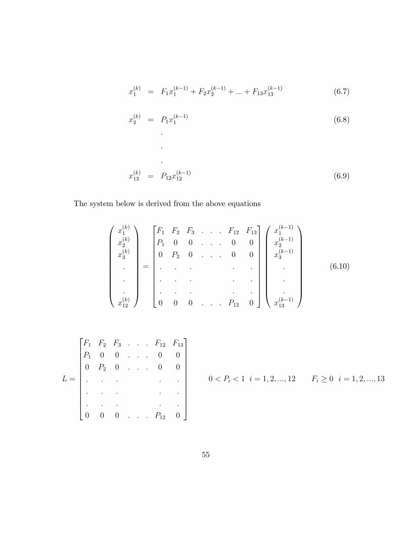
x(k)1 = F1x
(k�1)1 + F2x
(k�1)2 + :::+ F13x
(k�1)13 (6.7)
x(k)2 = P1x
(k�1)1 (6.8)
���
x(k)13 = P12x
(k�1)12 (6.9)
The system below is derived from the above equations
0BBBBBBBBBBB@
x(k)1
x(k)2
x(k)3
:
:
:
x(k)12
1CCCCCCCCCCCA=
2666666666664
F1 F2 F3 : : : F12 F13
P1 0 0 : : : 0 0
0 P2 0 : : : 0 0
: : : : :
: : : : :
: : : : :
0 0 0 : : : P12 0
3777777777775
0BBBBBBBBBBB@
x(k�1)1
x(k�1)2
x(k�1)3
:
:
:
x(k�1)13
1CCCCCCCCCCCA(6.10)
L =
2666666666664
F1 F2 F3 : : : F12 F13
P1 0 0 : : : 0 0
0 P2 0 : : : 0 0
: : : : :
: : : : :
: : : : :
0 0 0 : : : P12 0
37777777777750 < Pi < 1 i = 1; 2; :::; 12 Fi � 0 i = 1; 2; :::; 13
55
Assumptions
We will assume that for Amboseli elephants :
� The individuals in each group always go to the next group from one time step
to the next
� The survival and reproductive rates are constant over time within each ageclass and are therefore not dependent on population density
� The dynamics of the population are determined largely by females. We assumethat there will always be enough males to fertilize the females and therefore
the bulls do not play a major role in projecting the population
� Territory remains the same and is closed to migration. This implies that nomigration of elephants to and out of the park.
6.2.5 Parameter estimation
Data is extracted from a study by Cynthia Moss (2001) on Amboseli elephants.
Amboseli elephants life table is shown below
56
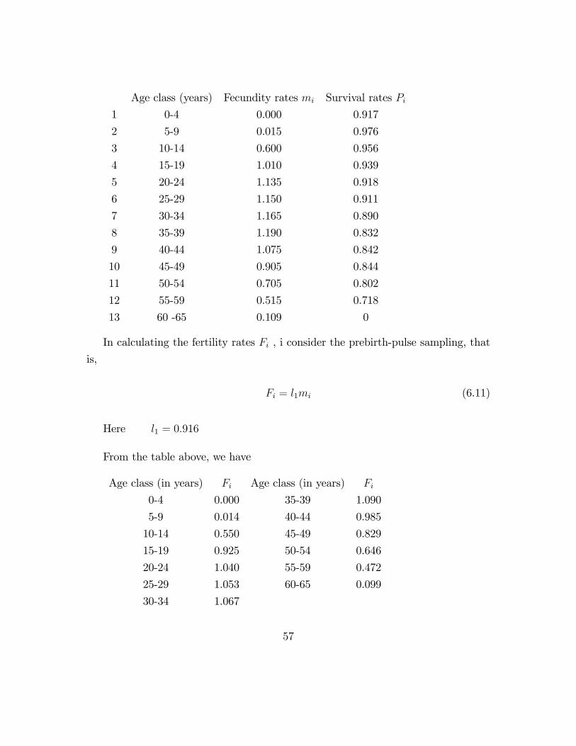
Age class (years) Fecundity rates mi Survival rates Pi1 0-4 0.000 0.917
2 5-9 0.015 0.976
3 10-14 0.600 0.956
4 15-19 1.010 0.939
5 20-24 1.135 0.918
6 25-29 1.150 0.911
7 30-34 1.165 0.890
8 35-39 1.190 0.832
9 40-44 1.075 0.842
10 45-49 0.905 0.844
11 50-54 0.705 0.802
12 55-59 0.515 0.718
13 60 -65 0.109 0
In calculating the fertility rates Fi , i consider the prebirth-pulse sampling, that
is,
Fi = l1mi (6.11)
Here l1 = 0:916
From the table above, we have
Age class (in years) Fi Age class (in years) Fi
0-4 0.000 35-39 1.090
5-9 0.014 40-44 0.985
10-14 0.550 45-49 0.829
15-19 0.925 50-54 0.646
20-24 1.040 55-59 0.472
25-29 1.053 60-65 0.099
30-34 1.067
57
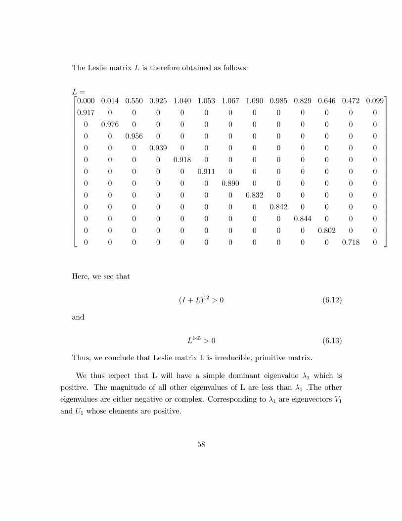
The Leslie matrix L is therefore obtained as follows:
L =2666666666666666666666666664
0:000 0:014 0:550 0:925 1:040 1:053 1:067 1:090 0:985 0:829 0:646 0:472 0:099
0:917 0 0 0 0 0 0 0 0 0 0 0 0
0 0:976 0 0 0 0 0 0 0 0 0 0 0
0 0 0:956 0 0 0 0 0 0 0 0 0 0
0 0 0 0:939 0 0 0 0 0 0 0 0 0
0 0 0 0 0:918 0 0 0 0 0 0 0 0
0 0 0 0 0 0:911 0 0 0 0 0 0 0
0 0 0 0 0 0 0:890 0 0 0 0 0 0
0 0 0 0 0 0 0 0:832 0 0 0 0 0
0 0 0 0 0 0 0 0 0:842 0 0 0 0
0 0 0 0 0 0 0 0 0 0:844 0 0 0
0 0 0 0 0 0 0 0 0 0 0:802 0 0
0 0 0 0 0 0 0 0 0 0 0 0:718 0
3777777777777777777777777775
Here, we see that
(I + L)12 > 0 (6.12)
and
L145 > 0 (6.13)
Thus, we conclude that Leslie matrix L is irreducible, primitive matrix.
We thus expect that L will have a simple dominant eigenvalue �1 which is
positive. The magnitude of all other eigenvalues of L are less than �1 .The other
eigenvalues are either negative or complex. Corresponding to �1 are eigenvectors V1and U1 whose elements are positive.
58
Chapter 7
Results and analysis
Here, we intend to carry out the following analysis:
a) Transient analysis: This focusses on the short-run behavior
b) Asymptotic analysis: This asks what happens if the life processes operate
for a very long time. What is the long-run behaviour of population? Does it grow,
decline or remain stationary?
c) Ergodicity : A model is said to be ergodic if its asymptotic dynamics are
independent of initial conditions
d) Perturbation analysis: Here, we ask what would happen to some dependent
variable if one or more independent variables were to change
7.0.6 Transient analysis
Matlab programming
Matlab programming is used to project future elephant population. First, we run
projection for the next 8 time steps to be able to see the trend and thereafter observe
population trend in the long run by considering many years. Here, what is of interest
59
is the stable population. This is the behavior of population in the long run where
we consider future proportions according to age classes. Population projection are
also represented in graphs for easier observation.
First, we follow the changes in the �rst 7 steps of time. This is done by starting
from zero and end with step 8. There are 13 age classes to deal with in each iteration.
We begin by inserting the Leslie matrix L , then prepare matlab to accommodate the
�rst seven time steps by inserting a null matrix. The null matrix will have 13 rows to
represent each of the 13 age classes and columns columns to accommodate population
for the �rst seven time steps. The �rst column contains the initial population vector.
Population in the year 1990 is taken to be the initial vector
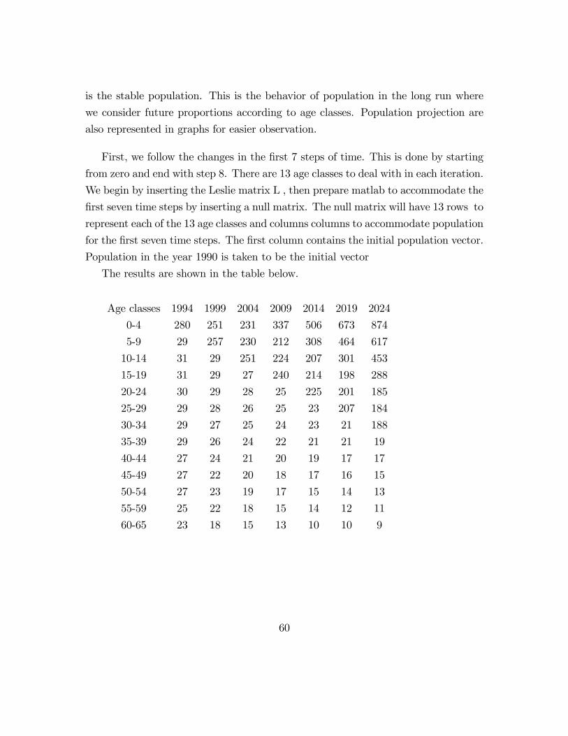
The results are shown in the table below.
Age classes 1994 1999 2004 2009 2014 2019 2024
0-4 280 251 231 337 506 673 874
5-9 29 257 230 212 308 464 617
10-14 31 29 251 224 207 301 453
15-19 31 29 27 240 214 198 288
20-24 30 29 28 25 225 201 185
25-29 29 28 26 25 23 207 184
30-34 29 27 25 24 23 21 188
35-39 29 26 24 22 21 21 19
40-44 27 24 21 20 19 17 17
45-49 27 22 20 18 17 16 15
50-54 27 23 19 17 15 14 13
55-59 25 22 18 15 14 12 11
60-65 23 18 15 13 10 10 9
60
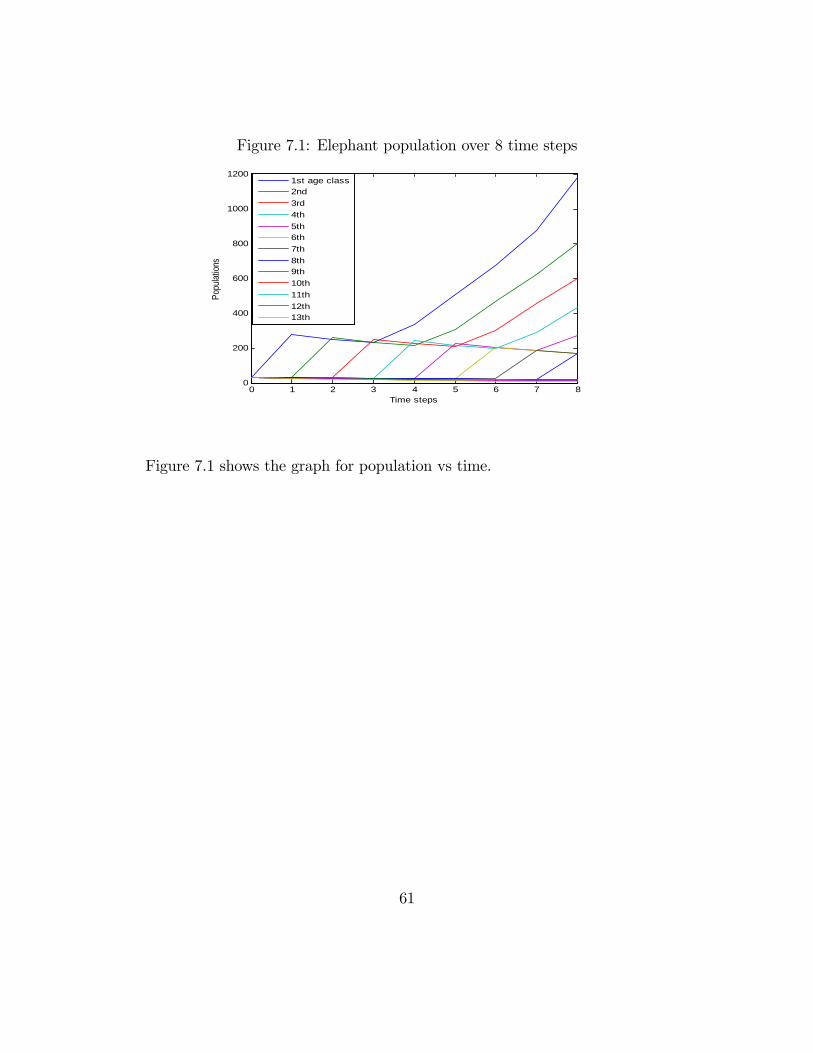
Figure 7.1: Elephant population over 8 time steps
0 1 2 3 4 5 6 7 80
200
400
600
800
1000
1200
Time steps
Popu
lation
s
1st age class2nd3rd4th5th6th7th8th9th10th11th12th13th
Figure 7.1 shows the graph for population vs time.
61
0 1 2 3 4 5 6 7 8100
101
102
103
104
Time steps
Log(
Pop
ulat
ion
1st age class2nd3rd4th5th6th7th8th9th10th11th12th13th
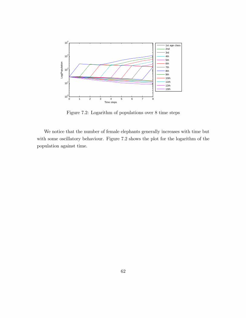
Figure 7.2: Logarithm of populations over 8 time steps
We notice that the number of female elephants generally increases with time but
with some oscillatory behaviour. Figure 7.2 shows the plot for the logarithm of the
population against time.
62
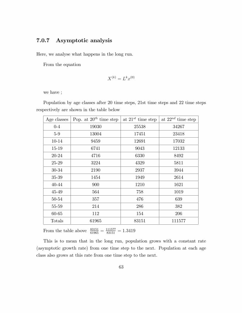
7.0.7 Asymptotic analysis
Here, we analyse what happens in the long run.
From the equation
X(k) = Lkx(0)
we have ;
Population by age classes after 20 time steps, 21st time steps and 22 time steps
respectively are shown in the table below
Age classes Pop. at 20th time step at 21st time step at 22nd time step
0-4 19030 25538 34267
5-9 13004 17451 23418
10-14 9459 12691 17032
15-19 6741 9043 12133
20-24 4716 6330 8492
25-29 3224 4329 5811
30-34 2190 2937 3944
35-39 1454 1949 2614
40-44 900 1210 1621
45-49 564 758 1019
50-54 357 476 639
55-59 214 286 382
60-65 112 154 206
Totals 61965 83151 111577
From the table above 8315161965
= 11157783151
= 1:3419
This is to mean that in the long run, population grows with a constant rate
(asymptotic growth rate) from one time step to the next. Population at each age
class also grows at this rate from one time step to the next.
63
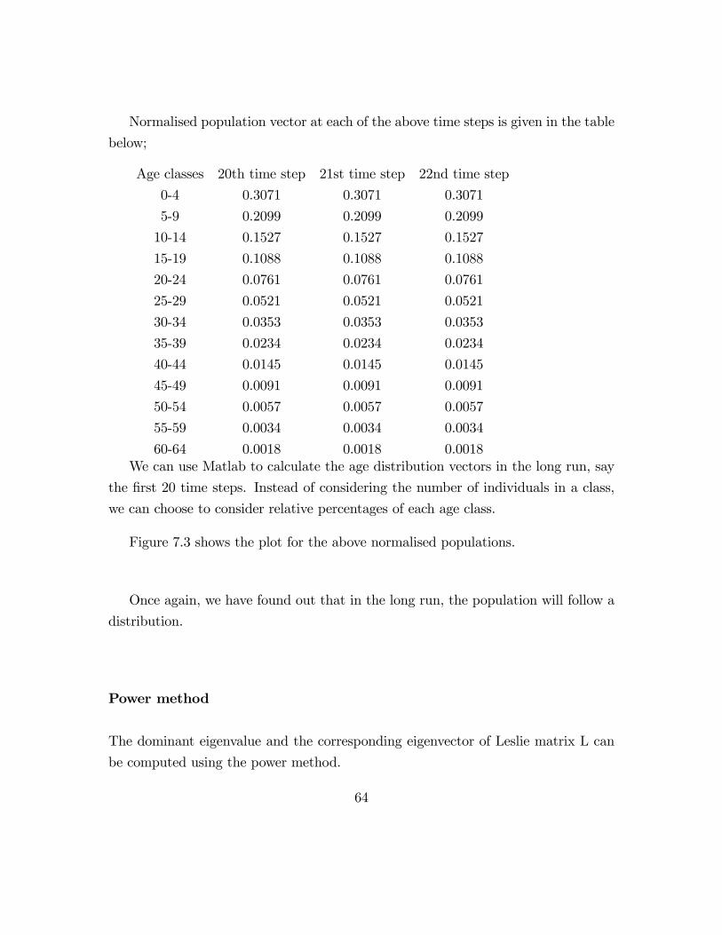
Normalised population vector at each of the above time steps is given in the table
below;
Age classes 20th time step 21st time step 22nd time step
0-4 0.3071 0.3071 0.3071
5-9 0.2099 0.2099 0.2099
10-14 0.1527 0.1527 0.1527
15-19 0.1088 0.1088 0.1088
20-24 0.0761 0.0761 0.0761
25-29 0.0521 0.0521 0.0521
30-34 0.0353 0.0353 0.0353
35-39 0.0234 0.0234 0.0234
40-44 0.0145 0.0145 0.0145
45-49 0.0091 0.0091 0.0091
50-54 0.0057 0.0057 0.0057
55-59 0.0034 0.0034 0.0034
60-64 0.0018 0.0018 0.0018We can use Matlab to calculate the age distribution vectors in the long run, say
the �rst 20 time steps. Instead of considering the number of individuals in a class,
we can choose to consider relative percentages of each age class.
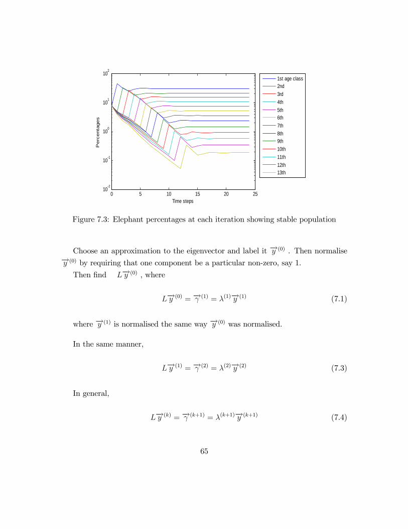
Figure 7.3 shows the plot for the above normalised populations.
Once again, we have found out that in the long run, the population will follow a
distribution.
Power method
The dominant eigenvalue and the corresponding eigenvector of Leslie matrix L can
be computed using the power method.
64
0 5 10 15 20 2510-2
10-1
100
101
102
Time steps
Perc
enta
ges
1st age class2nd3rd4th5th6th7th8th9th10th11th12th13th
Figure 7.3: Elephant percentages at each iteration showing stable population
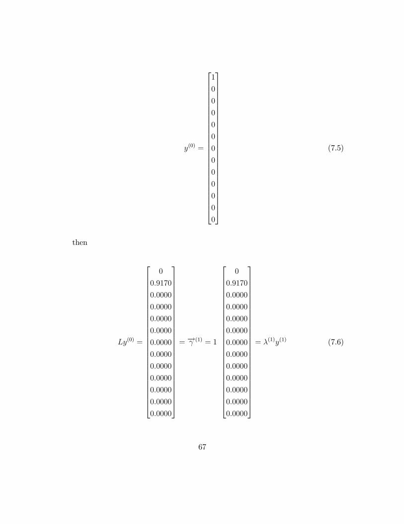
Choose an approximation to the eigenvector and label it �!y (0) . Then normalise�!y (0) by requiring that one component be a particular non-zero, say 1.Then �nd L�!y (0) , where
L�!y (0) = �! (1) = �(1)�!y (1) (7.1)
where �!y (1) is normalised the same way �!y (0) was normalised.
In the same manner,
L�!y (1) = �! (2) = �(2)�!y (2) (7.3)
In general,
L�!y (k) = �! (k+1) = �(k+1)�!y (k+1) (7.4)
65
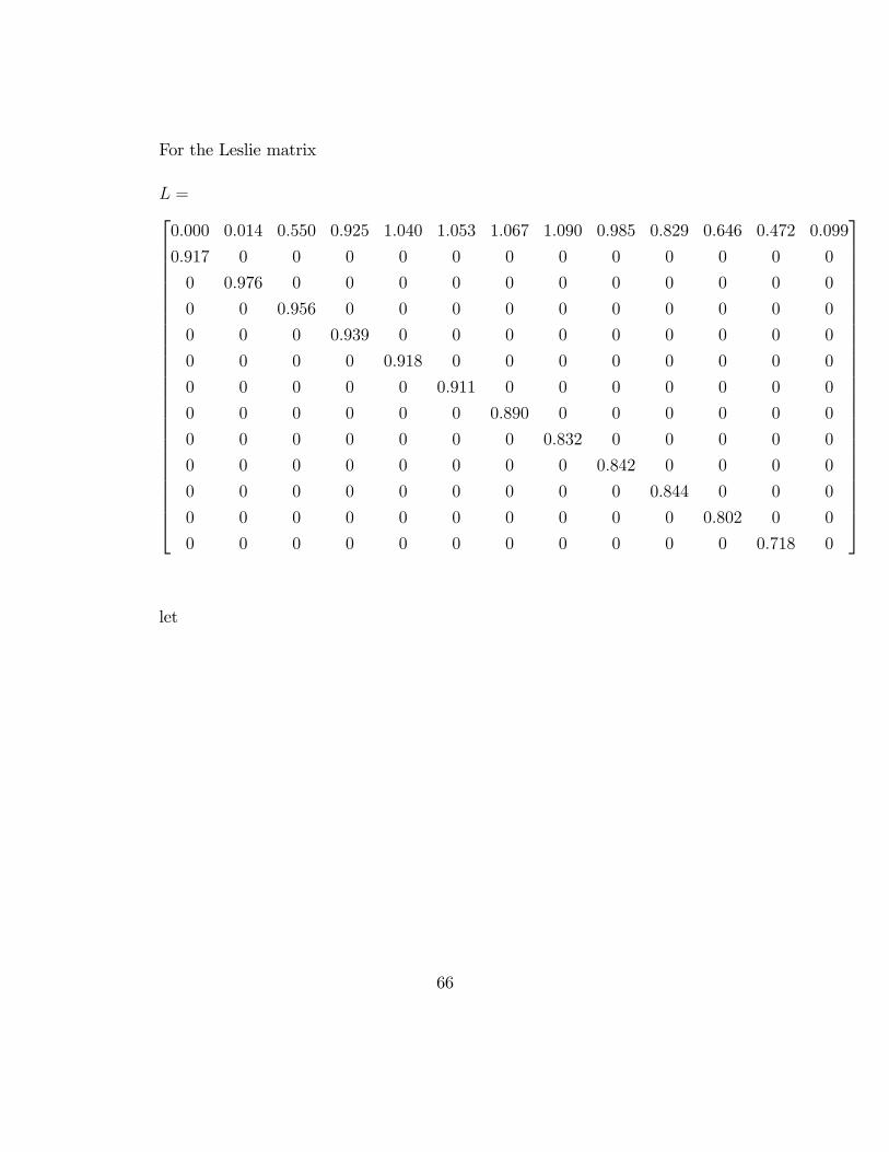
For the Leslie matrix
L =2666666666666666666666666664
0:000 0:014 0:550 0:925 1:040 1:053 1:067 1:090 0:985 0:829 0:646 0:472 0:099
0:917 0 0 0 0 0 0 0 0 0 0 0 0
0 0:976 0 0 0 0 0 0 0 0 0 0 0
0 0 0:956 0 0 0 0 0 0 0 0 0 0
0 0 0 0:939 0 0 0 0 0 0 0 0 0
0 0 0 0 0:918 0 0 0 0 0 0 0 0
0 0 0 0 0 0:911 0 0 0 0 0 0 0
0 0 0 0 0 0 0:890 0 0 0 0 0 0
0 0 0 0 0 0 0 0:832 0 0 0 0 0
0 0 0 0 0 0 0 0 0:842 0 0 0 0
0 0 0 0 0 0 0 0 0 0:844 0 0 0
0 0 0 0 0 0 0 0 0 0 0:802 0 0
0 0 0 0 0 0 0 0 0 0 0 0:718 0
3777777777777777777777777775
let
66
y(0) =
2666666666666666666666666664
1
0
0
0
0
0
0
0
0
0
0
0
0
3777777777777777777777777775
(7.5)
then
Ly(0) =
2666666666666666666666666664
0
0:9170
0:0000
0:0000
0:0000
0:0000
0:0000
0:0000
0:0000
0:0000
0:0000
0:0000
0:0000
3777777777777777777777777775
= �! (1) = 1
2666666666666666666666666664
0
0:9170
0:0000
0:0000
0:0000
0:0000
0:0000
0:0000
0:0000
0:0000
0:0000
0:0000
0:0000
3777777777777777777777777775
= �(1)y(1) (7.6)
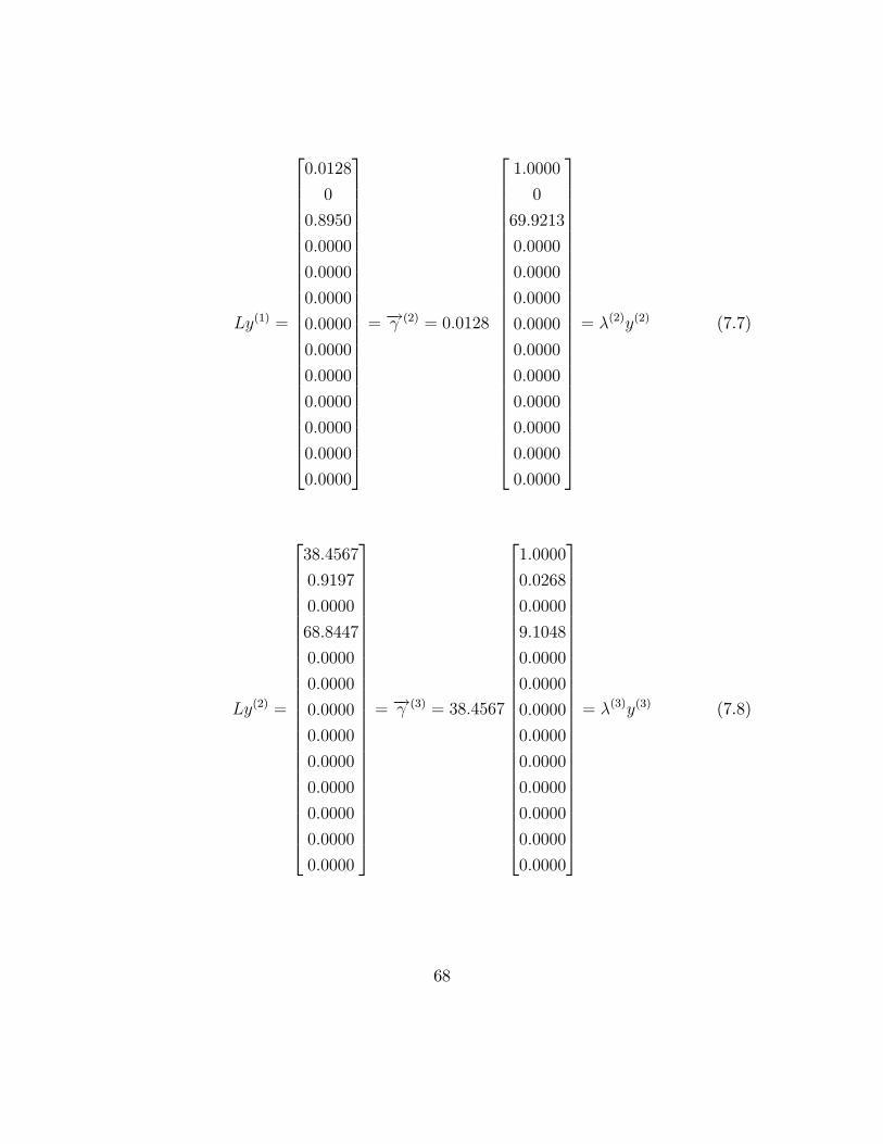
67
Ly(1) =
2666666666666666666666666664
0:0128
0
0:8950
0:0000
0:0000
0:0000
0:0000
0:0000
0:0000
0:0000
0:0000
0:0000
0:0000
3777777777777777777777777775
= �! (2) = 0:0128
2666666666666666666666666664
1:0000
0
69:9213
0:0000
0:0000
0:0000
0:0000
0:0000
0:0000
0:0000
0:0000
0:0000
0:0000
3777777777777777777777777775
= �(2)y(2) (7.7)
Ly(2) =
2666666666666666666666666664
38:4567
0:9197
0:0000
68:8447
0:0000
0:0000
0:0000
0:0000
0:0000
0:0000
0:0000
0:0000
0:0000
3777777777777777777777777775
= �! (3) = 38:4567
2666666666666666666666666664
1:0000
0:0268
0:0000
9:1048
0:0000
0:0000
0:0000
0:0000
0:0000
0:0000
0:0000
0:0000
0:0000
3777777777777777777777777775
= �(3)y(3) (7.8)
68
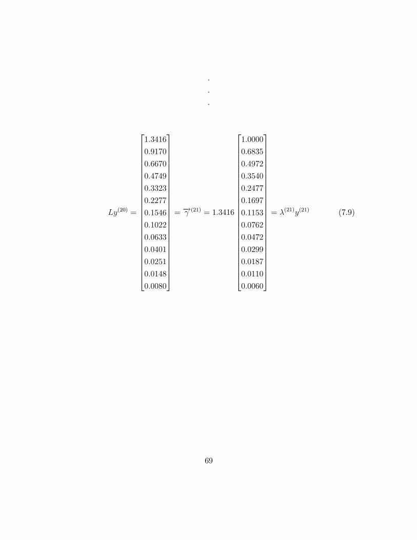
���
Ly(20) =
2666666666666666666666666664
1:3416
0:9170
0:6670
0:4749
0:3323
0:2277
0:1546
0:1022
0:0633
0:0401
0:0251
0:0148
0:0080
3777777777777777777777777775
= �! (21) = 1:3416
2666666666666666666666666664
1:0000
0:6835
0:4972
0:3540
0:2477
0:1697
0:1153
0:0762
0:0472
0:0299
0:0187
0:0110
0:0060
3777777777777777777777777775
= �(21)y(21) (7.9)
69
Ly(21) =
2666666666666666666666666664
1:3419
0:9170
0:6671
0:4753
0:3324
0:2274
0:1546
0:1026
0:0634
0:0397
0:0252
0:0150
0:0079
3777777777777777777777777775
= �! (22) = 1:3419
2666666666666666666666666664
1:0000
0:6833
0:4971
0:3542
0:2477
0:1694
0:1152
0:0765
0:0472
0:0296
0:0188
0:0112
0:0059
3777777777777777777777777775
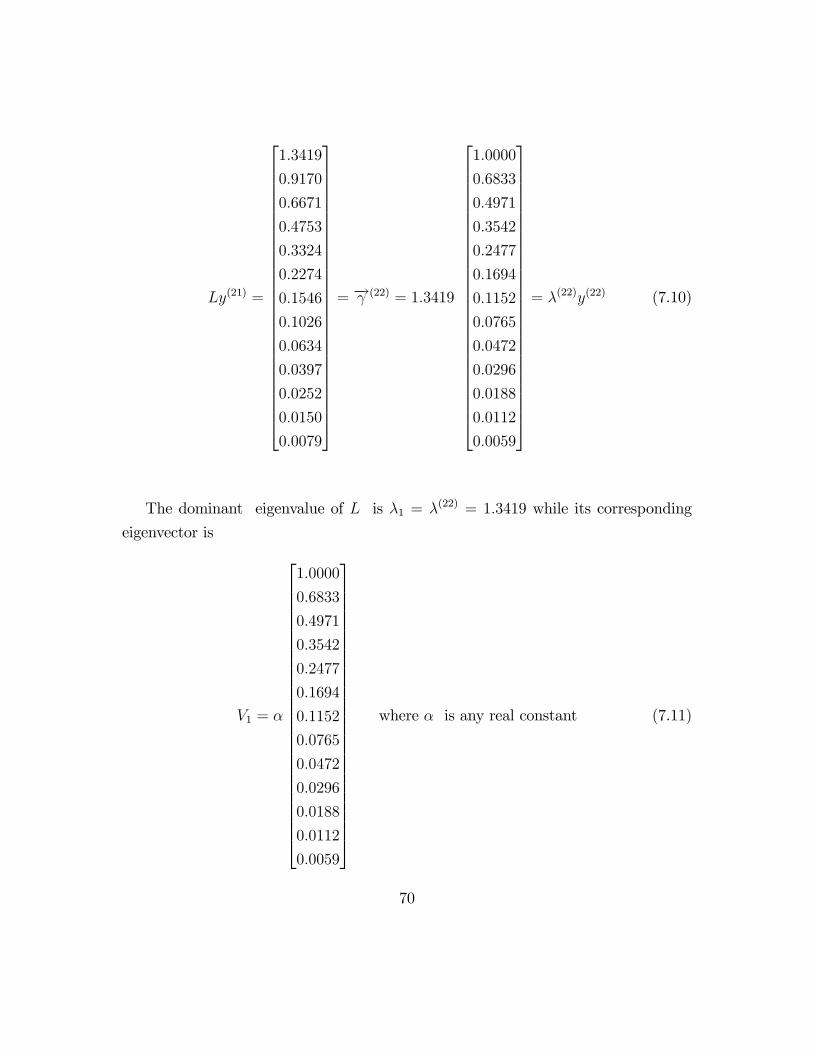
= �(22)y(22) (7.10)
The dominant eigenvalue of L is �1 = �(22) = 1:3419 while its corresponding
eigenvector is
V1 = �
2666666666666666666666666664
1:0000
0:6833
0:4971
0:3542
0:2477
0:1694
0:1152
0:0765
0:0472
0:0296
0:0188
0:0112
0:0059
3777777777777777777777777775
where � is any real constant (7.11)
70
To arrive at the eigenvalues and corresponding eigenvectors directly, we use Mat-
lab programming .
The eigenvalues of matrix L are listed below
�1 = 1:3419 (7.12)
�2; �3 = 0:5964� 0:5585i (7.13)
�4; �5 = 0:2692� 0:7524i (7.15)
�6; �7 = �0:0293� 0:8560i (7.16)
�8; �9 = �0:4021� 0:6491i (7.17)
�10 = �0:7471 (7.18)
�11; �12 = �0:6292� 0:3769i (7.19)
�13 = �0:2050 (7.20)
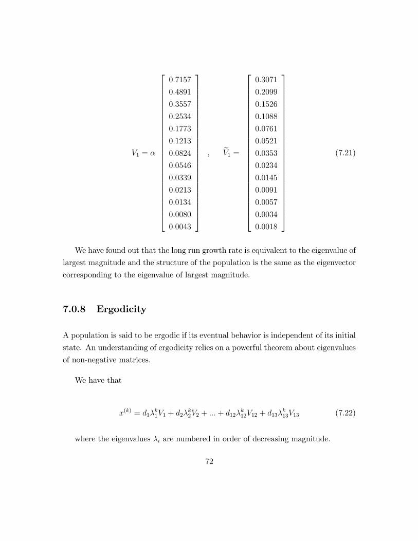
The eigenvector corresponding to the eigenvalue � = 1:3419 is V1 below. The
normalised eigenvector corresponding to � = 1:3419 is eV1 which is also shown below.
71
V1 = �
2666666666666666666666666664
0:7157
0:4891
0:3557
0:2534
0:1773
0:1213
0:0824
0:0546
0:0339
0:0213
0:0134
0:0080
0:0043
3777777777777777777777777775
, eV1 =
2666666666666666666666666664
0:3071
0:2099
0:1526
0:1088
0:0761
0:0521
0:0353
0:0234
0:0145
0:0091
0:0057
0:0034
0:0018
3777777777777777777777777775
(7.21)
We have found out that the long run growth rate is equivalent to the eigenvalue of
largest magnitude and the structure of the population is the same as the eigenvector
corresponding to the eigenvalue of largest magnitude.
7.0.8 Ergodicity
A population is said to be ergodic if its eventual behavior is independent of its initial
state. An understanding of ergodicity relies on a powerful theorem about eigenvalues
of non-negative matrices.
We have that
x(k) = d1�k1V1 + d2�
k2V2 + :::+ d12�
k12V12 + d13�
k13V13 (7.22)
where the eigenvalues �i are numbered in order of decreasing magnitude.
72
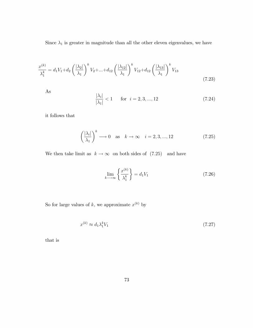
Since �1 is greater in magnitude than all the other eleven eigenvalues, we have
x(k)
�k1= d1V1+d2
�j�2j�1
�kV2+:::+d12
�j�12j�1
�kV12+d12
�j�13j�1
�kV13
(7.23)
Asj�ijj�1j
< 1 for i = 2; 3; :::; 12 (7.24)
it follows that
�j�ij�1
�k�! 0 as k !1 i = 2; 3; :::; 12 (7.25)
We then take limit as k !1 on both sides of (7:25) and have
limk�!1
�x(k)
�k1
�= d1V1 (7.26)
So for large values of k, we approximate x(k) by
x(k) � d1�k1V1 (7.27)
that is
73
x(k) � d1(1:3419)k
2666666666666666666666666664
0:7157
0:4891
0:3557
0:2534
0:1773
0:1213
0:0824
0:0546
0:0339
0:0213
0:0134
0:0080
0:0043
3777777777777777777777777775
(7.28)
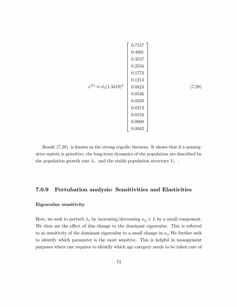
Result (7:28) is known as the strong ergodic theorem. It shows that if a nonneg-
ative matrix is primitive, the long-term dynamics of the population are described by
the population growth rate �1 and the stable population structure V1 .
7.0.9 Pertubation analysis: Sensitivities and Elasticities
Eigenvalue sensitivity
Here, we seek to perturb �1 by increasing/decreasing aij 2 L by a small component.We then see the e¤ect of this change to the dominant eigenvalue. This is referred
to as sensitivity of the dominant eigenvalue to a small change in aij:We further seek
to identify which parameter is the most sensitive. This is helpful in management
purposes where one requires to identify which age category needs to be taken care of
74
in order to prevent the overall population from being extinct. It also serves to know
which elephant category to avoid hunting in an event where hunting is legally allowed.
On the other hand,in an event of explosion in population, sensitivity analysis may
give information on which elephant category (with respect to age) should be removed
during harvesting in order to check on the population growth.
The formula for eigenvalue sensitivity is
S =
�@�1@aij
�(7.29)
Eigenvalue elasticity
Survival probabilies does not exceed 1 but fertility rates have no restriction ,that is,
not bounded above. If the di¤erences between survival rates and fertility rates are
too big, then sensitivity analysis may not give a very reliable information. Here it
will be useful to consider the e¤ect of a proportional change of parameters to the
dominant eigenvalue. For example how much change to the dominant eigenvalue
will be caused by increasing fertility or survival rates by some proportion. The
proportional response to a proportional perturbation is known as elasticity.
The elasticities of � with respect to the element aij 2 L are often interpreted asthe contributions of each of the aij to � .
Eigenvalue elasticity is expressed as
eij =aij�
@�
@aij(7.30)
The table below shows sensitivities and elasticities of the dominant eigenvalue of
matrix L (�1 = 1:3419) to a small change in di¤erent parameters:
75
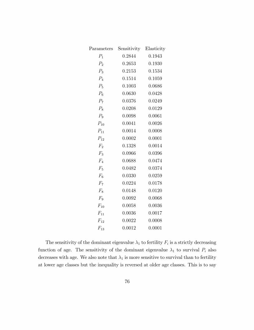
Parameters Sensitivity Elasticity
P1 0:2844 0:1943
P2 0:2653 0:1930
P3 0:2153 0:1534
P4 0:1514 0:1059
P5 0:1003 0:0686
P6 0:0630 0:0428
P7 0:0376 0:0249
P8 0:0208 0:0129
P9 0:0098 0:0061
P10 0:0041 0:0026
P11 0:0014 0:0008
P12 0:0002 0:0001
F2 0:1328 0:0014
F3 0:0966 0:0396
F4 0:0688 0:0474
F5 0:0482 0:0374
F6 0:0330 0:0259
F7 0:0224 0:0178
F8 0:0148 0:0120
F9 0:0092 0:0068
F10 0:0058 0:0036
F11 0:0036 0:0017
F12 0:0022 0:0008
F13 0:0012 0:0001
The sensitivity of the dominant eigenvalue �1 to fertility Fi is a strictly decreasing
function of age. The sensitivity of the dominant eigenvalue �1 to survival Pi also
decreases with age. We also note that �1 is more sensitive to survival than to fertility
at lower age classes but the inequality is reversed at older age classes. This is to say
76
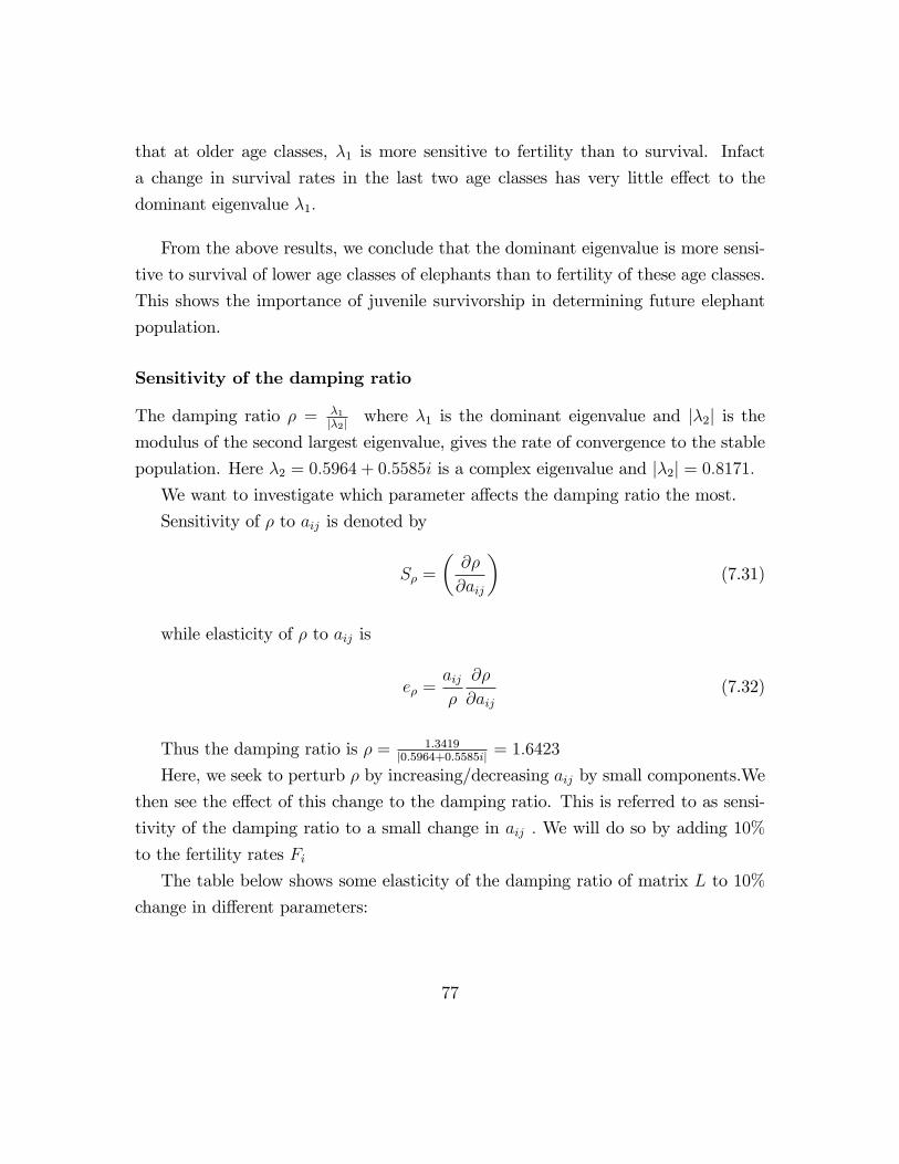
that at older age classes, �1 is more sensitive to fertility than to survival. Infact
a change in survival rates in the last two age classes has very little e¤ect to the
dominant eigenvalue �1:
From the above results, we conclude that the dominant eigenvalue is more sensi-
tive to survival of lower age classes of elephants than to fertility of these age classes.
This shows the importance of juvenile survivorship in determining future elephant
population.
Sensitivity of the damping ratio
The damping ratio � = �1j�2j where �1 is the dominant eigenvalue and j�2j is the
modulus of the second largest eigenvalue, gives the rate of convergence to the stable
population. Here �2 = 0:5964 + 0:5585i is a complex eigenvalue and j�2j = 0:8171:We want to investigate which parameter a¤ects the damping ratio the most.
Sensitivity of � to aij is denoted by
S� =
�@�
@aij
�(7.31)
while elasticity of � to aij is
e� =aij�
@�
@aij(7.32)
Thus the damping ratio is � = 1:3419j0:5964+0:5585ij = 1:6423
Here, we seek to perturb � by increasing/decreasing aij by small components.We
then see the e¤ect of this change to the damping ratio. This is referred to as sensi-
tivity of the damping ratio to a small change in aij : We will do so by adding 10%
to the fertility rates FiThe table below shows some elasticity of the damping ratio of matrix L to 10%
change in di¤erent parameters:
77
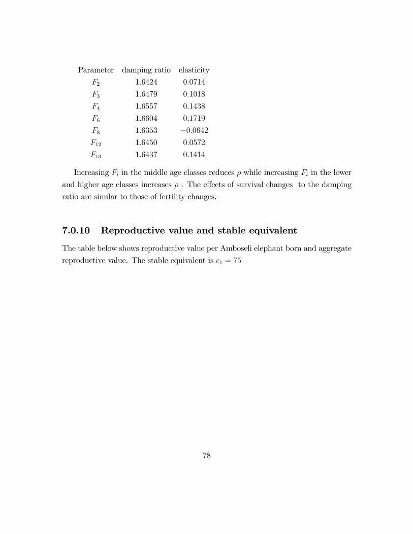
Parameter damping ratio elasticity
F2 1:6424 0:0714
F3 1:6479 0:1018
F4 1:6557 0:1438
F6 1:6604 0:1719
F8 1:6353 �0:0642F12 1:6450 0:0572
F13 1:6437 0:1414
Increasing Fi in the middle age classes reduces � while increasing Fi in the lower
and higher age classes increases � . The e¤ects of survival changes to the damping
ratio are similar to those of fertility changes.
7.0.10 Reproductive value and stable equivalent
The table below shows reproductive value per Amboseli elephant born and aggregate
reproductive value. The stable equivalent is c1 = 75
78
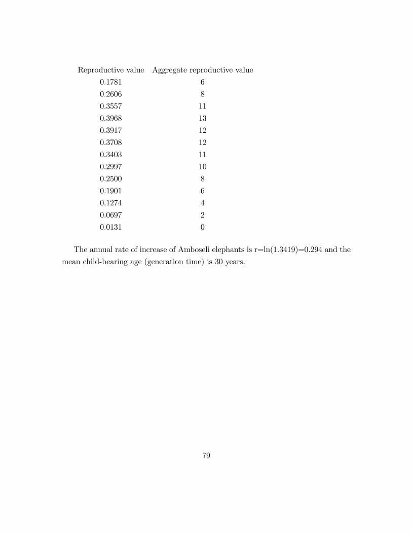
Reproductive value Aggregate reproductive value
0.1781 6
0.2606 8
0.3557 11
0.3968 13
0.3917 12
0.3708 12
0.3403 11
0.2997 10
0.2500 8
0.1901 6
0.1274 4
0.0697 2
0.0131 0
The annual rate of increase of Amboseli elephants is r=ln(1.3419)=0.294 and the
mean child-bearing age (generation time) is 30 years.
79
Chapter 8
Incorporating density dependenceinto the Leslie matrix model
A case of density independent Leslie matrix model has been considered above and
the general trend is that the elephant population increases with time and in the long
run population dynamics is an increment with a constant factor from one time step
to the next. This is basic model that seeks to get the overall trend of population
dynamics.
Due to limitation of Amboseli National park in terms of resources and competition
among elephants, the population will not grow inde�nately with time and thus there
is a need to incorporate density dependence into the model.This will ensure that in
the long run, elephant population will not grow inde�nately. Any incorporation of
density dependence decreases the vital rates.
There are several ways of incorporating density dependence and hereby, one way
is discussed. We consider density as the sum of all individuals in the population
irrespective of their ages. Let this sum be x(k), where
x(k) =Xi
x(k)i where x(k)i is the number of individuals at age class i during time step k
(8.1)
80
Now, let Pi and Fi be variables and not costants because they will be a¤ected by
the density. As the population increases, the survival rate Pi will decrease. This is
because of increased competition of resources among elephants. To ensure that this
is true, we de�ne a quantity q such that Pi is a decreasing function.
Let
q = 1 + �x(k) (8.2)
where � = ��1Kis a density parameter. � is the asymptotic growth rate considering
density independence, K is the carrying capacity of the park.
Arrange the quantity q such it forms the diagonal element of an n � n matrixQ, that is,
Q =
26666666664
q1(t) o � � � 0
0 q2(t) 0 � � 0
� � �� � �� � 0
0 0 � � 0 qn(t)
37777777775(8.3)
We divide matrix L by this quantity Q and have that at time at time k+1,
x(k+1) = LQ�1x(k) (8.4)
This means that the new Leslie matrix will have its vital rates divided by the
quantity q.
8.1 Analysis of the density parameter �
If � = 0, then q = 1 and thus we have density independence as discussed earlier.
If � < 0, then q < 1 with necessarily no lower bound. This will lead to negative
entries in the vital rates of the new Leslie matrix. This will invalidate the model
81
because ordinarily, projection matrices are supposed to be non-negative.
The only viable option is to have � > 0 . This means that q(t) > 1
After several projections,the population will reach stability say at time � .Thus,
from q = 1 + �x(k) , we have
q = 1 + (�� 1K
)x(k)
= 1 + (�� 1K
)K
= 1 + (�� 1)= � (8.5)
and the new Leslie matrix becomes
L =
2666666666664
F1�
F2�
F3�
: : : F12�
F13�
P1�
0 0 : : : 0 0
0 P2�
0 : : : 0 0
: : : : :
: : : : :
: : : � : :
0 0 0 : : : P12�
0
3777777777775(8.6)
0 < Pi < 1 i = 1; 2; :::; 12
Fi � 0 i = 1; 2; :::; 13
8.2 Results
This model shows that elephant population increases with up to a certain time where
the population becomes constant, that is, with no growth rate. This is where the
82
park has attained its carrying capacity and will therefore not accommodate more
elephants. Infact, the dominant eigenvalue of the new Leslie matrix is 1 .
83
Chapter 9
Findings and recommendations
9.1 Findings
The Leslie matrix L largely depends on two vital rates: fertility and survival rates.
This matrix is used to describe the population dynamics of Amboseli elephants by
calculating its eigenvalues and corresponding eigenvectors.
A time-invariant and density independent system was �rst considered. Here,
the Leslie matrix elements are considered to be constant over time. The elephant
population is grouped into uniform age classes where individuals in the same age class
are assumed to have almost similar characteristics. Each individual in a particular
age class is considered to have the same chance of surviving from its current age class
to the next. All populations are considered to move to the next age class during the
next time interval.
It is noted that all elephants age classes, except the �rst one, are productive.
The extreme age classes however, have lower productivity. The most productive age
classes are those in the middle.
Four types of analysis are carried out.
Transient analysis: Here, short-run behaviour of Amboseli elephants is observed.
The population is observed to be generally on the increase with oscillatory motion.
84
In order to visualise this well, a graph of population with time is sketched.
Asymptotic analysis: Long-run population dynamics is analysed. It is noted that
the population of Amboseli elephants increase with time in all the age classes. A close
look at the behaviour of increment shows that from one time interval to the next,
the population in all the age classes increases with a constant factor. This constant
factor is what is referred to as asymptotic growth rate. In an attempt to �nd out
what this growth rate would mean with respect to the matrix L, the eigenvalues of
the matrix were calculated.
Since L is a nonnegative, irreducible matrix, it will possess ( using Perron Frobe-
nius theorem) an eigenvalue which is greatest in magnitude compared to all the
other eigenvalues. This eigenvalue is termed as the dominant eigenvalue of matrix
L. A famous method of calculating this dominant eigenvalue is called power method.
The dominant eigenvalue is found to be 1.3419 . The other 12 eigenvalues were got
by programming using Matlab software. They are either negative or complex. It is
noted that the asymptotic growth rate is indeed the dominant eigenvalue of matrix
L .
Another feature of the long-run population dynamics is the stable age distribu-
tion.The population is observed to grow proportionally in the long run. That is, the
percentages of elephants in each and every age class is constant. Once again, these
proportions are the same as the right eigenvector corresponding to the dominant
eigenvalue of matrix L .
Ergodicity: It is found out that the long run population dynamics does not
depend on the initial population vector but only on the dominant eigenvalue and its
corresponding eigenvector. The fact that we can use any population vector as the
initial vector and still arrive at stable population is an important thing to note in
population modelling.
Perturbation analysis: It is noted that the sensitivity of the dominant eigenvalue
to fertility rates Fi is a decreasing function. The sensitivity of the dominant eigen-
value to survival rates Pi is also a decreasing function. This is to say that the growth
rate is more sensitive to changes in survival and fertility rates at younger age classes
than older age classes of Amboseli elephants. A small change in Fi and Pi at younger
85
age classes will cause greater impact to the asymptotic growth rate than when the
change is applied to older age classes. If one needs to cause some bigger changes to
the growth rate, then it should be applied to the lower age classes. The asymptotic
growth rate is also more sensitive to survival rates than fertility rates at younger age
classes but is more sensitive to fertility rates than survival rates at older age classes.
Damping ratio � refers to the rate of convergence to the stable population. Increas-
ing Fi in the lower and higher age classes of Amboseli elephants increases the rate
of convergnce to the stable population. Increasing Fi in the middle age classes re-
duce the rate of convergence to the stable population. An explanation of this is that
increasing Fi at the middle age classes would begin to make fertility periodic with
respect to age, which will slow down convergence to the stable population. E¤ects
of changing survival rates are similar to those of fertility changes.
Incorporation of density dependence was also considered. Density was de�ned to
be the total population of individuals irrespective of their age classes. Incorporation
of density dependence was found to decrease the vital rates and hence the asymptotic
growth rate. Once the population attains an equilibrium ( carrying capacity of the
park), the population in all the age classes remain constant at any time thereafter.
9.2 Recommendation
In this study, we have mostly concentrated on density independent Leslie matrix
model and later incorporated some density dependence with respect to total popula-
tion. As an extension to this study, i intend to fully incorporate density dependence
by also including e¤ects of di¤erent climatic conditions to population dynamics of
Amboseli elephants. Interraction between elephants and the environment (vegetation
in the park) and competition of resources among elephants will also be considered.
The model analysed was to a higher extent linear.The e¤ects of nonlinear terms have
not been addressed. This needs to be incorporated in order to make the model more
realistic.
86
References
[1] C. J Moss, The Demography of an African Elephant(Loxodonta africana) pop-
ulation in Amboseli, Kenya,2001
[2] D. W Jordan and P. Smith,Nonlinear ODE: Problems and solutions,2007,Oxford
Univerity Press Inc
[3] D. Arnold, Kevin Yokoyama, The Leslie Matrix Linear Algebra
[4] Edgar Ouko and Fredrick Onyango ,Fluctuations in Leslie matrix parameters
and their e¤ect on the stable population stucture, Vol3, Issue 11, International
Journal of Current Research,2011
[5] H. Caswell, Matrix Population Models:Construction, Analysis and Interpreta-
tion, 2nd ed.,Sinauer Associates Inc.,2001
[6] J. D Murray, Mathematical Biology: An Introduction, 3rd ed, vol 17
[7] J.R Chasnow,Mathematical Biology, Hong-Kong University of Science and Tech-
nology,2009
[8] Manuela L. de Castro, J.A.L Silva,D.A.R Justo,Stability in an age-structured
metapopulation model,2005,J Math Biol.
[9] M.Marva,A. Moussaoui,R.Bravo de la Parra,P. Auger,A density dependent
model describing age-structured population dynamics using hawk-dove tac-
tics,2012, Journal of Di¤erence Equations and Applications.
87
[10] Mosimanegape Irvin Montshiwa,Leslie Matrix model in Population Dynam-
ics,2007
[11] N. Key�tz, Mathematical Demography
[12] P.H Leslie,On the use of Matrices in Certain Population Mathematics,Vol 33,
No. 3, Biometrica Trust
[13] R. Clubb, M. Rowcli¤e,P.Lee,C.Moss,G. Mason,Fecundity and population via-
bility in female zoo elephants,Animal Welfare,2009
[14] Samy Gallego, Modelling Population Dynamics of Elephants,2003
[15] Wen-Ching Li, Application of Leslie matrix models to wild turkey populations,
1994
[16] W.Sprague, Automatic parametrization of age/sex Leslie matrices for human
population,2012
88
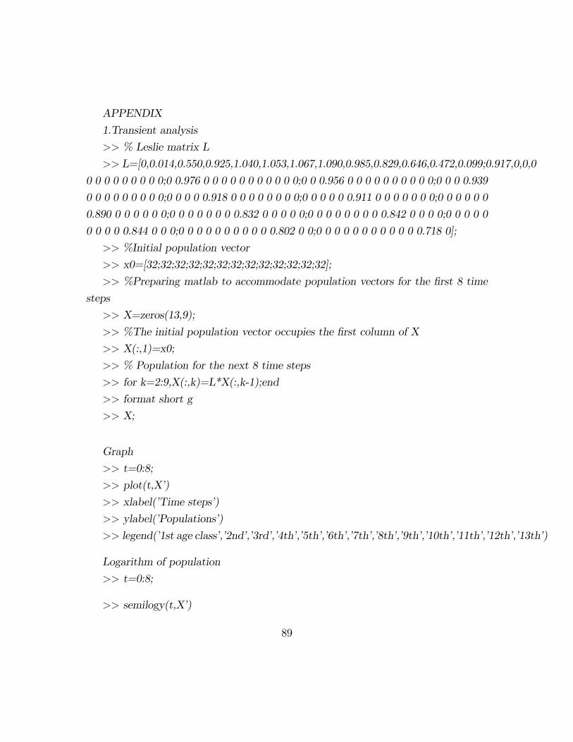
APPENDIX
1.Transient analysis
>> % Leslie matrix L
>> L=[0,0.014,0.550,0.925,1.040,1.053,1.067,1.090,0.985,0.829,0.646,0.472,0.099;0.917,0,0,0
0 0 0 0 0 0 0 0 0;0 0.976 0 0 0 0 0 0 0 0 0 0 0;0 0 0.956 0 0 0 0 0 0 0 0 0 0;0 0 0 0.939
0 0 0 0 0 0 0 0 0;0 0 0 0 0.918 0 0 0 0 0 0 0 0;0 0 0 0 0 0.911 0 0 0 0 0 0 0;0 0 0 0 0 0
0.890 0 0 0 0 0 0;0 0 0 0 0 0 0 0.832 0 0 0 0 0;0 0 0 0 0 0 0 0 0.842 0 0 0 0;0 0 0 0 0
0 0 0 0 0.844 0 0 0;0 0 0 0 0 0 0 0 0 0 0.802 0 0;0 0 0 0 0 0 0 0 0 0 0 0.718 0];
>> %Initial population vector
>> x0=[32;32;32;32;32;32;32;32;32;32;32;32;32];
>> %Preparing matlab to accommodate population vectors for the �rst 8 time
steps
>> X=zeros(13,9);
>> %The initial population vector occupies the �rst column of X
>> X(:,1)=x0;
>> % Population for the next 8 time steps
>> for k=2:9,X(:,k)=L*X(:,k-1);end
>> format short g
>> X;
Graph
>> t=0:8;
>> plot(t,X�)
>> xlabel(�Time steps�)
>> ylabel(�Populations�)
>> legend(�1st age class�,�2nd�,�3rd�,�4th�,�5th�,�6th�,�7th�,�8th�,�9th�,�10th�,�11th�,�12th�,�13th�)
Logarithm of population
>> t=0:8;
>> semilogy(t,X�)
89
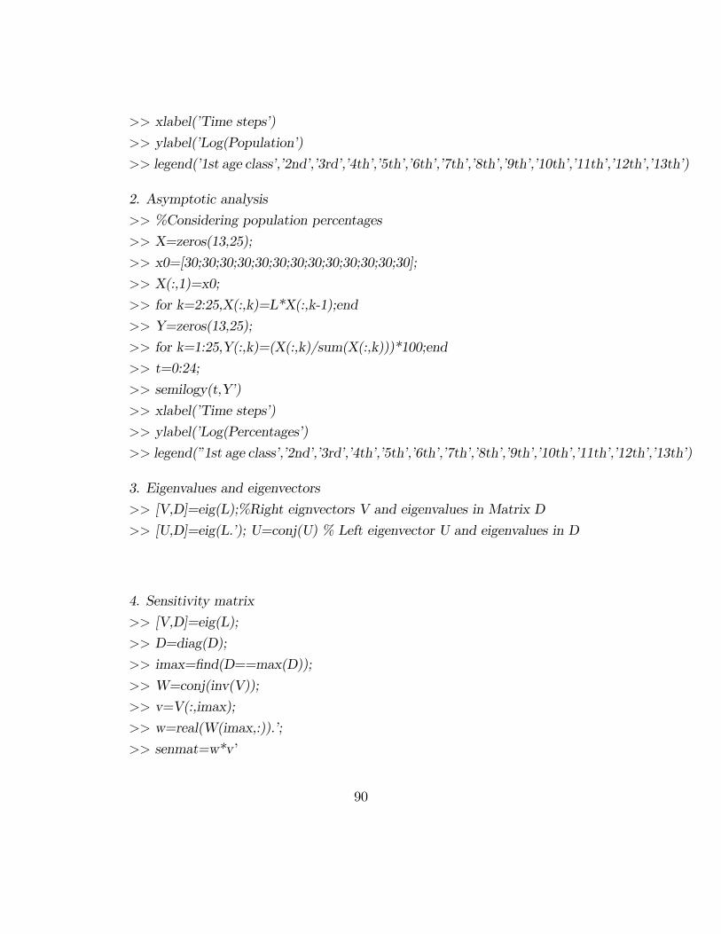
>> xlabel(�Time steps�)
>> ylabel(�Log(Population�)
>> legend(�1st age class�,�2nd�,�3rd�,�4th�,�5th�,�6th�,�7th�,�8th�,�9th�,�10th�,�11th�,�12th�,�13th�)
2. Asymptotic analysis
>> %Considering population percentages
>> X=zeros(13,25);
>> x0=[30;30;30;30;30;30;30;30;30;30;30;30;30];
>> X(:,1)=x0;
>> for k=2:25,X(:,k)=L*X(:,k-1);end
>> Y=zeros(13,25);
>> for k=1:25,Y(:,k)=(X(:,k)/sum(X(:,k)))*100;end
>> t=0:24;
>> semilogy(t,Y�)
>> xlabel(�Time steps�)
>> ylabel(�Log(Percentages�)
>> legend(�1st age class�,�2nd�,�3rd�,�4th�,�5th�,�6th�,�7th�,�8th�,�9th�,�10th�,�11th�,�12th�,�13th�)
3. Eigenvalues and eigenvectors
>> [V,D]=eig(L);%Right eignvectors V and eigenvalues in Matrix D
>> [U,D]=eig(L.�); U=conj(U) % Left eigenvector U and eigenvalues in D
4. Sensitivity matrix
>> [V,D]=eig(L);
>> D=diag(D);
>> imax=�nd(D==max(D));
>> W=conj(inv(V));
>> v=V(:,imax);
>> w=real(W(imax,:)).�;
>> senmat=w*v�
90


