HAL Id: hal-00656048https://hal.inria.fr/hal-00656048

Submitted on 3 Jan 2012

HAL is a multi-disciplinary open accessarchive for the deposit and dissemination of sci-entific research documents, whether they are pub-lished or not. The documents may come fromteaching and research institutions in France orabroad, or from public or private research centers.

L’archive ouverte pluridisciplinaire HAL, estdestinée au dépôt et à la diffusion de documentsscientifiques de niveau recherche, publiés ou non,émanant des établissements d’enseignement et derecherche français ou étrangers, des laboratoirespublics ou privés.

Constructing and Visualizing Chemical ReactionNetworks from Pi-Calculus Models

Mathias John, Hans-Jörg Schulz, Heidrun Schumann, Adelinde Uhrmacher,Andrea Unger

To cite this version:Mathias John, Hans-Jörg Schulz, Heidrun Schumann, Adelinde Uhrmacher, Andrea Unger. Con-structing and Visualizing Chemical Reaction Networks from Pi-Calculus Models. Formal Aspects ofComputing, Springer Verlag, 2012, �10.1007/s00165-011-0209-0�. �hal-00656048�

Under consideration for publication in Formal Aspects of Computing

Constructing and VisualizingChemical Reaction Networks fromPi-Calculus ModelsMathias John1, Hans-Jorg Schulz2, Heidrun Schumann3, Adelinde M. Uhrmacher3, and

Andrea Unger4

1BioComputing, Lifl (Cnrs Umr8022) & Iri (Cnrs Usr3078) & University of Lille 1, France2Graz University of Technology, Austria3University of Rostock, Germany4Helmholtz Centre Potsdam, Germany

Abstract. The π-calculus, in particular its stochastic version the stochastic π-calculus, is a common mod-eling formalism to concisely describe the chemical reactions occurring in biochemical systems. However, itremains largely unexplored how to transform a biochemical model expressed in the stochastic π-calculusback into a set of meaningful reactions. To this end, we present a two step approach of first translatingmodel states to reaction sets and then visualizing sequences of reaction sets, which are obtained from statetrajectories, in terms of reaction networks. Our translation from model states to reaction sets is formallydefined and shown to be correct, in the sense that it reflects the states and transitions as they are derivedfrom the continuous time Markov chain-semantics of the stochastic π-calculus. Our visualization conceptcombines high level measures of network complexity with interactive, table-based network visualizations.It directly reflects the structures introduced in the first step and allows modelers to explore the resultingsimulation traces by providing both: an overview of a network’s evolution and a detail inspection on demand.

Keywords: pi-calculus, stochastic modeling, reaction networks, graph visualization

Correspondence and offprint requests to:Mathias John,Interdisciplinary Research Institute,Parc de la Haute Borne, 50 avenue de Halley, BP 7047859658 Villeneuve d’Ascq Cedex, FRANCE.e-mail: mathias.john@lifl.fr

1. Introduction

Over the last years, computational modeling became a valuable method to study the dynamics of complexcell-biological systems. The idea is to provide an abstract representation of the system under study, ex-pressed in a modeling formalism, and to analyze such with the help of computers. By this, computationalmodeling helps to structure knowledge, to evaluate existing theories, and to suggest new set-ups for wet-labexperiments.

The π-calculus [Mil99] is considered to be a well-suited formalism for the modeling of cell-biologicalprocesses [Reg03, PRSS01]. Its stochastic version, called the stochastic π-calculus [Pri95], comes with astochastic semantics in terms of continuous time Markov chains (ctmc) that allows to account for thedynamics of cell-biological processes. The stochastic π-calculus has been applied in several modeling studies,see for example, [Kut06, TK08, CCG+09, MJM+09]. However, due to the origin of the π-calculus in the fieldof concurrency theory, the basic paradigm of the stochastic π-calculus is the one of process communication,whereas cell-biological systems are rather described in terms of chemical reactions and solutions. Therefore,efforts have been made to find ways of transforming reaction networks into process communication, seee.g., [PRSS01, Kut06].

The way back from stochastic π-calculus models to chemical reactions, however, is largely unexplored.But it is this half of the modeling cycle that actually allows modelers to review whether the transformationfrom reactions to process communication yields the desired results and whether the model is a meaningfulinterpretation in the biochemical context. To this end, we propose a two-step approach of first extractingreaction sets from stochastic π-calculus models and then visualizing the obtained results in terms of reactionnetworks. Thereby, the size of resulting reaction sets forms the major challenge. Each of a stochastic π-calculus model’s ctmc states defines a set of chemical reactions that may possibly occur. Existing approachestry to create reaction sets accounting for all states of a model at once [Car08a, Car08b, MG09]. In practicalcases, this, however, mostly leads to reaction sets of large, up to infinite size (a detailed example and alsoan introduction to the stochastic π-calculus can be found in Section 2). Therefore, we propose an approachthat considers each model state individually. Timed traces of model states are obtained based on stochasticsimulation in terms of [Gil77]. This first step of our approach is presented in Section 3.

To support model analysis across multiple consecutive states of a simulation, we propose the secondstep of visualization. Reaction sets of individual states are represented in a time-dependent manner, suchthat the dynamics of the transformed model are easily accessible. By making use of a representation asreaction networks, our visualization is capable of handling individual reaction sets of large size. Withouta systematic visual approach for their representation and exploration, experts may theoretically be able tounderstand the results of the transformation, but practically drown in them. Previous attempts of visualizingstochastic π-calculus models are either mere static graphical notations [PCC06] or do not scale well tolarge models because of the chosen visualization approach of a 3-dimensional spatial layout [Phi]. In bothcases, the visualizations do not reflect the nature of a reaction network and stick closely to the notion ofcommunicating automata. Hence, in Section 4, we propose a visualization setup that is more scalable byemploying more space-efficient visualization methods, such as an overview, which summarizes the distinctstates of the solution using measures of network complexity, and table-based representations for a detailedview of individual states. By this, the exploration of these large data sets is visually supported and themodeler can finally draw the needed conclusions from the transformation results – be it during the actualmodeling phase in which the model must be debugged and validated, or while working with the model togain an understanding of the inner workings of the modeled cell-biological system.

It is notable that our approach is not only applicable to the stochastic π-calculus, but also to most of itsextensions. We provide a brief discussion on this topic in Section 5, before concluding this paper by givingan outlook on directions for future work in Section 6.

2. The Stochastic π-Calculus

We base our investigation on the biochemical form of the stochastic π-calculus. This is a reformulation of thestochastic π-calculus that is closer to the field of modeling biochemical systems, in the sense that it providesnotions of molecules and chemical solutions rather than just accounting for concurrently acting processes(achieved by syntactic restrictions). The two existing up-to-date stochastic π-calculus tools for modeling

2

Fig. 1. Binding reaction between three different sorts of molecules. Molecule A may perform an un-/binding reaction withB by creating and removing links (black line) between binding sites s1 and s. Similarly, molecules A and C may bind usingrespective binding sites s2 and s. Dashed lines represent links that may be present but do not have to be. That is, reactions onsite s1 may happen independently of the state of site s2 and vv. This means the following chemical reactions can take place:A,B ←→ AB; AC,B ←→ ACB; A,C ←→ AC; AB,C ←→ ABC.

biochemical systems base on the biochemical form [PC07, LJU10]. In the following, when mentioning thestochastic π-calculus, we actually refer to its biochemical form.

The idea of modeling chemical reactions in the stochastic π-calculus is, instead of using rather monolithicspecies for complexes like ABC, to describe a complex of three molecules A, B, and C, to actually considermolecules with their individual binding sites and complexes by establishing links between them, see Figure 1.As shown in [HFB+03, FHR+03], this view may significantly increase the conciseness of model descriptions.For this, the stochastic π-calculus requires modelers to shift their focus from reactions to molecules andtheir interactions. Consider, e.g., the complex formations depicted in Figure 1. These can be modeled in thestochastic π-calculus in the following way:

A( s1 , s2 , s1N , s2N ) =: s1 ! ( s1N ) .A( s1N , s2 , s1 , s2N )+ s2 ! ( s2N ) .A( s1 , s2N , s1N , s2 )

B( s ) =: s ?( sN ) .B( sN)C( s ) =: s ?( sN ) .C( sN )

Molecule definitions are introduced for A,B,C with parameters s1,s2,s,s1N,s2N. The only values in the stochas-tic π-calculus are names, also called channels. Interaction capabilities between molecules, i.e., the reactionsthat may possibly occur, depend on name scoping. For example, a chemical solution with one A and two B, allnot bound, can be denoted as the parallel composition of molecules S = A(bAB,bAC,uAB,uAC) | B(bAB) | B(bAB).The idea is that molecule A(bAB,bAC,uAB,uAC) shares the name bAB as the value of its first parameter with allB(bAB), allowing for free interaction between all A and B. By contrast, a solution S′ = A(uAB,bAC,bAB,uAC) |B(uAB) | B(bAB) is to denote a complex of A with the first B, since only these two may interact on channel uAB.In the very same way, interaction capabilities between A and C molecules can be controlled, using names bAC

and uAC. Whereas interactions on channels bAB, bAC shall model binding reactions, those on channels uAB,uACare considered to denote unbinding reactions. This is specified in the definitions of the respective molecules.The only notion of interaction in the stochastic π-calculus is the one of communication, with one sendingand one receiving partner. Molecules A(bAB,bAC,uAB,uAC) and B(bAB) can send (!) and receive (?) on channelbAB, respectively. As denoted in the parentheses after the !-operator, A(bAB,bAC,uAB,uAC) sends channel bAB

to B(bAB) that addresses it with formal parameter bNext. After their interaction, A(bAB,bAC,uAB,uAC) is to bereplaced by A(uAB,bAC,bAB,uAC) and B(bAB) by B(uAB). Thus, interactions on channel B(bAB) denote a bindingbetween A and B, as they lead from solution S above to solution S′. Subsequently, A(uAB,bAC,bAB,uAC) andB(uAB) may communicate on channel uAB in the very same way to be replaced again by A(bAB,bAC,uAB,uAC)

and B(bAB), thus denoting the unbinding by closing the cycle from S′ to S. Alternatively, as denoted by thechoice operator (+), A(bAB,bAC,uAB,uAC) can perform the very same interactions, just on channels bAC anduAC, with C(bAC). Notice, that this happens entirely independently of the values of parameters s1 and s1N.Thus, a solution S = A(bAB,bAC,uAB,uAC) | B(bAB) | C(bAC) represents by the interaction capabilities of itscontained molecules the following eight chemical reactions that in fact reflect those depicted in Figure 1:

A(bAB,bAC,uAB,uAC),B(bAB) ←→ A(uAB,bAC,bAB,uAC),B(uAB)

A(bAB,uAC,uAB,bAC),B(bAB) ←→ A(uAB,uAC,bAB,bAC),B(uAB)

A(bAB,bAC,uAB,uAC), C(bAC) ←→ A(bAB,uAC,uAB,bAC), C(uAC)

A(uAB,bAC,bAB,uAC), C(bAC) ←→ A(uAB,uAC,bAB,bAC), C(uAC)

Notice, that we actually need to distinguish reactions based on the parameter values of their reactants,since, e.g., A(bAB,bAC,uAB,uAC) has different interaction capabilities then A(uAB,bAC,bAB,uAC). In fact, one canconsider A(bAB,bAC,uAB,uAC) and A(uAB,bAC,bAB,uAC) to be of a different chemical species, just like A andAB. Notice further that our model so far only works in the presence of a single A molecule. Consider,e.g., a solution S = A(uAB,bAC,bAB,uAC) | A(uAB,bAC,bAB,uAC) | B(uAB) | B(uAB). Here the scope of uAB is not

3

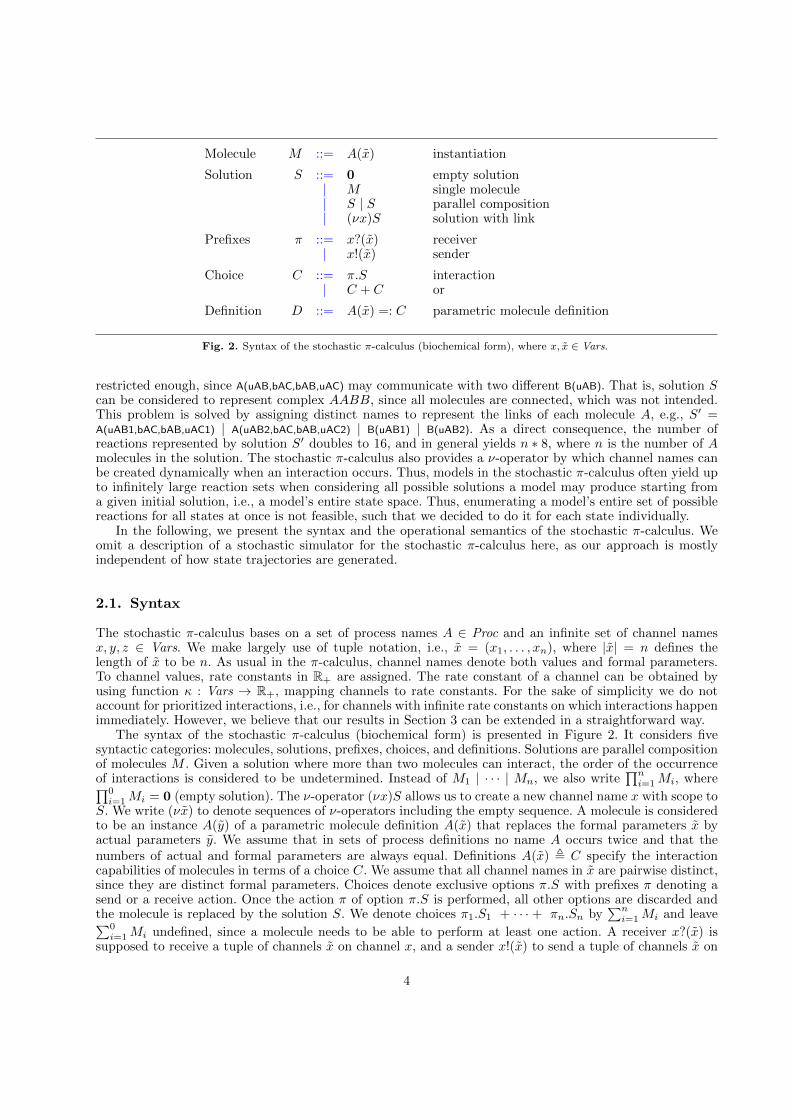
Molecule M ::= A(x) instantiation

Solution S ::= 0 empty solution| M single molecule| S | S parallel composition| (νx)S solution with link

Prefixes π ::= x?(x) receiver| x!(x) sender

Choice C ::= π.S interaction| C + C or

Definition D ::= A(x) =: C parametric molecule definition

Fig. 2. Syntax of the stochastic π-calculus (biochemical form), where x, x ∈ Vars.

restricted enough, since A(uAB,bAC,bAB,uAC) may communicate with two different B(uAB). That is, solution Scan be considered to represent complex AABB, since all molecules are connected, which was not intended.This problem is solved by assigning distinct names to represent the links of each molecule A, e.g., S′ =A(uAB1,bAC,bAB,uAC1) | A(uAB2,bAC,bAB,uAC2) | B(uAB1) | B(uAB2). As a direct consequence, the number ofreactions represented by solution S′ doubles to 16, and in general yields n ∗ 8, where n is the number of Amolecules in the solution. The stochastic π-calculus also provides a ν-operator by which channel names canbe created dynamically when an interaction occurs. Thus, models in the stochastic π-calculus often yield upto infinitely large reaction sets when considering all possible solutions a model may produce starting froma given initial solution, i.e., a model’s entire state space. Thus, enumerating a model’s entire set of possiblereactions for all states at once is not feasible, such that we decided to do it for each state individually.

In the following, we present the syntax and the operational semantics of the stochastic π-calculus. Weomit a description of a stochastic simulator for the stochastic π-calculus here, as our approach is mostlyindependent of how state trajectories are generated.

2.1. Syntax

The stochastic π-calculus bases on a set of process names A ∈ Proc and an infinite set of channel namesx, y, z ∈ Vars. We make largely use of tuple notation, i.e., x = (x1, . . . , xn), where |x| = n defines thelength of x to be n. As usual in the π-calculus, channel names denote both values and formal parameters.To channel values, rate constants in R+ are assigned. The rate constant of a channel can be obtained byusing function κ : Vars → R+, mapping channels to rate constants. For the sake of simplicity we do notaccount for prioritized interactions, i.e., for channels with infinite rate constants on which interactions happenimmediately. However, we believe that our results in Section 3 can be extended in a straightforward way.

The syntax of the stochastic π-calculus (biochemical form) is presented in Figure 2. It considers fivesyntactic categories: molecules, solutions, prefixes, choices, and definitions. Solutions are parallel compositionof molecules M . Given a solution where more than two molecules can interact, the order of the occurrenceof interactions is considered to be undetermined. Instead of M1 | · · · | Mn, we also write

∏ni=1Mi, where∏0

i=1Mi = 0 (empty solution). The ν-operator (νx)S allows us to create a new channel name x with scope toS. We write (νx) to denote sequences of ν-operators including the empty sequence. A molecule is consideredto be an instance A(y) of a parametric molecule definition A(x) that replaces the formal parameters x byactual parameters y. We assume that in sets of process definitions no name A occurs twice and that thenumbers of actual and formal parameters are always equal. Definitions A(x) , C specify the interactioncapabilities of molecules in terms of a choice C. We assume that all channel names in x are pairwise distinct,since they are distinct formal parameters. Choices denote exclusive options π.S with prefixes π denoting asend or a receive action. Once the action π of option π.S is performed, all other options are discarded andthe molecule is replaced by the solution S. We denote choices π1.S1 + · · · + πn.Sn by

∑ni=1Mi and leave∑0

i=1Mi undefined, since a molecule needs to be able to perform at least one action. A receiver x?(x) issupposed to receive a tuple of channels x on channel x, and a sender x!(x) to send a tuple of channels x on

4

fv(C1 + C2) = fv(C1) + fv(C2) fv(0) = ∅fv(x?(x).S) = {x} ∪ (fv(S) \ {y}) fv(S1 | S2) = fv(S1) ∪ fv(S2)fv(x!(y).S) = {x} ∪ fv({y}) ∪ fv(S) fv(A(x)) = {x} ∪ fv(A(x) , C)

fv((νx : k)S) = fv(S) \ {x} fv(A(x) , C) = fv(C) \ {x}

Fig. 3. Free channel names of the π-calculus with priority.

S1 | S2 ≡ S2 | S1 (S1 | S2) | S3 ≡ S1 | (S2 | S3)S | 0 ≡ S (νx)(S1 | S2) ≡ (νx)S1 | S2 if x 6∈ fv(S2)

S1 ≡α S2 ⇒ S1 ≡ S2 (νx1)(νx2)S ≡ (νx2)(νx1)S

Fig. 4. Axioms of the structural congruence of the π-calculus with priority.

channel x. We again assume that all channel names in y are pairwise distinct, since they are distinct formalparameters.

We introduce a structural congruence of solutions which is the least relation satisfying the rules in Fig-ure 4. It identifies all those solutions that satisfy associativity and commutativity. Furthermore, it allows usomitting empty solutions in parallel compositions. Moreover, it identifies solutions by consistently renamingbound names, i.e., using α-conversion. For this, it strongly relies on the function fv to determine free namesin solutions, see Figure 3. We consider all those names to be free which are not in the scope of ν-bindersor the formal parameters of molecule definitions and receive actions. Renaming operations also extend torate constant function κ. The structural congruence lets us change the order of ν-operators and extend theirscope to solutions whose free names do not equal the name bound by the ν-operator.

We say a solution S is in prenex normal form if and only if S = (νx)∏ni=1Mi. We introduce a multiset

representation of a prenex normal form by (νx) ·∏ni=1M

mii , where molecules Mi occur mi times. Notice,

that every solution is structurally congruent to a prenex normal form.

2.2. Operational semantics

The semantics of the stochastic π-calculus maps a solution S to a state of a continuous time Markov chain(ctmc) including its transitions. The main idea is to regard all distinct solutions which are reachable fromS as successor states. Thereby, two states are considered distinct if their solutions are not structurallycongruent. The transitions of S are derived from its possible communications, transition weights are obtainedby summing up the rate constants of all possible communications leading to the same successor state.As shown in, e.g., [KLN07], stochastic simulators can be derived directly from such stochastic π-calculussemantics.

In order to account for all possible communications in a solution, the semantics strongly relies ondetermining the redexes of prenex normal forms. Thereby, a redex of a solution in prenex normal formS = (νx)

∏ni=1Mi is defined as a tuple (i1, j1, i2, j2) that captures with i1, i2 ∈ {1, . . . , n} the indices of two

molecules forming an interaction pair, with Mi1 being the sender and Mi2 the receiver. By j1, j2 then, theindices of the actions in the choices defining Mi1 ,Mi2 that let Mi1 ,Mi2 communicate are reflected. Consider,e.g., solution S = A(b,b,u1,u2) | B(b) | B(b), with definitions as in our introducing example (also recalled inFigure 6). We obtain four redexes (1, 1, 2, 1), (1, 2, 2, 1), (1, 1, 3, 1), and (1, 2, 3, 1), accounting for all possiblecommunications in S.

The rules of the operational semantics of the stochastic π-calculus are presented in Figure 5. We denotethe substitution of tuple x by tuple y as [y/x]. Substitution only applies to tuples of the same length. Byrule (app) molecules are replaced by their definitions with the formal parameters being substituted by theactual ones. Rule (red) formulates the reduction of a pair of communicating molecules M1,M2. Therefore,it captures the indices i1, i2 of the actions that let M1,M2 communicate and the channel x on which theycommunicate. In order to ensure a proper substitution, it further checks whether M2 is actually ready toreceive the amount of values that M1 sends. Rule (sel) selects two molecules to communicate. Only thosepairs qualify to which rule (red) applies and that refer to distinct molecules, since one molecule may not

5

Application

(app)A(x) =: C

A(y)app−−→ C[y/x]

Communication

(red)M1

app−−→∑ni=1 πi.Si M2

app−−→∑n′

i=1 π′i.S′i πi1 = x!(x) π′i2 = x?(y) |x| = |y|

M1,M2x−−−−→

(i1,i2)Si1 | Si2

(sel)

Mi1 ,Mi2x−−−−→

(j1,j2)S i1 6= i2

(νx : k)∏ni=1Mi

x−−−−−−−→(i1,j1,i2,j2)

(νx : k)(∏ni=1,i6=i1,i2 Mi) | S

Markov chain

(sum)S ≡ S1

∑{(k,`)|S1

x−→S2,S2≡S′,k=κ(x)} k = r 6= 0

Sr−→ S′

Fig. 5. Rules of the stochastic semantics of the stochastic π-calculus (biochemical form).

A( s1 , s2 , s1N , s2N ) =:s1 ! ( s1N ) .A( s1N , s2 , s1 , s2N )

+ s2 ! ( s2N ) .A( s1 , s2N , s1N , s2 )

B( s ) =: s ?( sN ) .B( sN)

Fig. 6. The ctmc of solution S = A(b,b,u1,u2) | B(b)2, obtained following the rules of the operational semantics of the stochasticπ-calculus as presented in Figure 5.

communicate with itself. Communication transitions are annotated with communication channel x and redex`. This information is used to obtain state transitions in rule (sum), where state transitions are defined bycombining all communications that lead to the same successor and summing up corresponding rate constants.

For illustration, Figure 6 depicts the ctmc of solution S = A(b,b,u1,u2) | B(b)2, with molecule definitionsas in our introducing example (also recalled in the figure).

3. Extracting reaction sets from processes

In this section, we show how to extract reaction sets from solutions. We fix a notion of reactions that directly

follows the ideas given in Section 2. That is, an interaction M1 |M2x−−−−→

(j1,j2)S, with S ≡ (νx)

∏ni=1Mi yields

reaction M1,M2x−→ (νx)(M ′1, . . . ,M

′n). It may seem surprising that reactions are with a channel upon the

arrow and not with a rate constant as usual. However, the idea is that if modelers denote interactions tohappen on different channels, they also intend them to denote different reactions, even if they show the samerate constants.

In order to identify communications in a given solution, we introduce communication labels that comprisea communication’s channel, rate constant, and redex. More precisely, a communication label of a solution S is

a tuple ` = (x, i1, j1, i2, j2), where S′x−−−−−−−→

(i1,j1,i2,j2)S′′, with S′ ≡ S. The set Λ(S) contains all communication

6

labels of a solution S in prenex normal form and is defined as:

Λ(S) = {(x, i1, j1, i2, j2) | S x−−−−−−−→(i1,j1,i2,j2)

S′}, with S = (νx)

n∏i=1

Mi

Since two communications labels may refer to the same reaction, we need to ensure that we do not extractreaction duplicates. Therefore, we introduce an equivalence of communication labels ∼ that identifies twocommunication labels that refer to the same reaction. It is defined as the least relation fulfilling the followingrule:

(x, i1, j1, i2, j2) ∼ (x′, i′1, j′1, i′2, j′2)

if and only if

x = x′,Mi1 |Mi2 ≡Mi′1|Mi′2

,Mi1 |Mi2x−−−−→

(j1,j2)S,Mi′1

|Mi′2

x′−−−−→(j′1,j

′2)

S′ ≡ S

We define the quotient set of communication labels that contains the equivalent classes of the communicationlabels of solution S in the following way:

Λ∼(S) = {[`] | ` ∈ Λ(S)}, where [`] = {`′ ∈ Λ(S) | `′ ∼ `}

By definition, each equivalent class in Λ(S) represents a single reaction. The set of reactions of S canthus be obtained by picking a representative of each equivalent class in Λ∼(S). Consider, e.g., solutionS = A(b,b,u1,u2) | B(b) | B(b), with definitions as in our introducing example (also recalled in Figure 6). Weobtain Λ∼(S) = {{(b, 1, 1, 2, 1), (b, 1, 1, 3, 1)}, {(b, 1, 2, 2, 1), (b, 1, 2, 3, 1)}}, containing the equivalent classesrepresenting the two reactions:

A(b,b,u1,u2),B(b)b−→ A(u1,b,b,u2),B(u1)

A(b,b,u1,u2),B(b)b−→ A(b,u2,u1,b),B(u2)

Constructing Λ∼(S) from a given solution S requires a pairwise comparison of communication labels,yielding quadratic complexity in the number of communication labels in S. An increased performance can beachieved by making use of the fact that most π-calculus simulators, e.g., [PC07, LJU10], work with speciesset representations of solutions S = (νx) ·

∏ni=1M

mii . The idea is that a molecule pair M1,M2 shows the

same interaction capabilities as all other molecule pairs M ′1,M′2, where M1 = M ′1 and M2 = M ′2, i.e., where

M1 and M2 are of the species as M ′1 and M ′2, respectively. Thus, instead of considering S, one can extractthe set of reactions directly from solution S′ = (νx)

∏ni=1Mi. In most practical cases the number of species

will be considerably smaller then the number of molecules. We introduce the quotient set Λ∼• that allows usto extract reactions directly from species set representations as follows:

Λ∼• (S) = Λ∼((νx)

n∏i=1

Mi), with S ≡ (νx)

n

·∏i=1

Mmii

For illustration consider the solution S = A(b,b,u1,u2) | B(b)2 as in our preceding example. We obtain Λ∼• (S) ={{(b, 1, 1, 2, 1)}, {(b, 1, 2, 2, 1)}}, i.e., two equivalence classes representing the same reactions as before. Thefollowing lemma states that in general this way of extracting reaction sets is correct.

Lemma 1. For all solutions S in prenex normal form it holds that ]Λ∼(S) ⊆ ]Λ∼• (S) and for all [`] ∈ Λ∼(S),there exists exactly one [`′] ∈ Λ∼• (S), such that ` ∼ `′.

Proof. Let S ≡ (νx) ·∏ni=1M

mii , S′ = (νx)

∏ni=1Mi and S = (νx)

∏n′

i=1M′i . By definition, Λ∼• (S) = Λ∼(S′).

Thus, ]Λ∼(S) ⊆ ]Λ∼• (S)) clearly holds. Furthermore, assume that there exists no [`′] ∈ Λ∼• (S), such that

[`] ∼ [`′]. Let ` = (x, i1, j1, i2, j2) and M ′i1 | M′i2

(i1,j1,i2,j2)−−−−−−−→x

S1. By definition, there exists i′1, i′2, such that

M ′i1 = Mi′1and M ′i2 = Mi′2

. This implies that Mi′1| Mi′2

(i′1,j1,i′2,j2)−−−−−−−→

xS1, such that ` ∼ (x, i′1, j1, i

′2, j2).

Since ∼ is an equivalence relation, the definition of Λ∼ provides that there exists [`′] ∈ Λ∼(S′) with [`′] ∼(x, i′1, j1, i

′2, j2). By transitivity it also holds that `′ ∼ `, which contradicts our initial assumption. Moreover,

transitivity provides that there cannot exist [`′′] ∈ Λ(S′), with ` ∼ `′′ and `′ 6= `′′.

7

Given a solution S, the rates of reactions in Λ∼(S) can be easily determined by summing up therate constants of the communication labels belonging to the same equivalence class. However, when usingΛ∼• (S), where not all communication labels are individually considered, this is not feasible (e.g., Λ∼(S) ={{(b, 1, 1, 2, 1), (b, 1, 1, 3, 1)}, {(b, 1, 2, 2, 1), (b, 1, 2, 3, 1)}} vs.Λ∼• (S) = {{(b, 1, 1, 2, 1)}, {(b, 1, 2, 2, 1)}}, with Sas in the preceding examples). In this case reaction rates need to be determined more directly in the fol-lowing way: consider communication label ` = (x, i1, j1, i2, j2) and solution S ≡ (νx) ·

∏ni=1M

mii . By the

definition of ∼, all the communication labels belonging to [`] show the same rate constant. Thus, it sufficesto compute the number of communication labels `′ ∈ Λ(S), with `′ ∼ `. We start by counting the number ofcommunication labels `′ = (x, i′1, j1, i

′2, j2) in Λ(S), with Mi1 = Mi′1

and Mi2 = Mi′2. Following the rules of

combinatorics, this yields mi1 ∗mi2 , if Mi1 6= Mi2 and mi1 ∗ (mi2 −1) = mi1 ∗ (mi1 −1), otherwise. However,molecules Mi1 ,Mi2 may also be defined to perform the same reaction several times. For example, a pair ofmolecules D(), E(), with definitions D() =: x!().E() + x?().D() and E() =: x!().E() + x?().D(). By definition of Λ∼• ,all the communication labels involving Mi1 ,Mi2 , also those where Mi1 ,Mi2 swap the sending and receivingrole, are considered by [`] ∈ Λ∼• (S). Again, it is clear that all copies of Mi1 ,Mi2 behave the same way. Thus,we define the reaction rate of a communication label of solution S in the following way:

ρ(`, S) = κ(x) ∗ ][`] ∗ τ, where

τ =

{mi1 ∗ (mi2 − 1), if Mi1 = Mi2

mi2 ∗mi2 , else

and ` = (x, i1, j1, i2, j2), S ≡ (νx) ·∏ni=1M

mii , [`] ∈ Λ∼• (S)

Consider, e.g., solution S = A(b,b,u1,u2) | B(b)2 as in our preceding examples, where Λ∼(S) ={{(b, 1, 1, 2, 1), (b, 1, 1, 3, 1)}, {(b, 1, 2, 2, 1), (b, 1, 2, 3, 1)}} and Λ∼• (S) = {{(b, 1, 1, 2, 1)}, {(b, 1, 2, 2, 1)}}. Weobtain that κ((b, 1, 1, 2, 1), S) = κ((b, 1, 2, 2, 1), S) = 2κ(b). It remains to ensure that really all communi-cation labels `′ ∈ Λ(S), with `′ ∼ `, are take into account. The following lemma states that our way ofcomputing rates based Λ∼• is correct in general.

Lemma 2. Let S be a solution in prenex normal form. For all [`] ∈ Λ∼• (S), it holds that ρ(`, S) =∑{(x,l)|(x,l)∈Λ(S),(x,l)∼`} κ(x).

Proof. Let ` = (x, i1, j1, i2, j2) and ∆ = {`′ | `′ ∈ Λ(S), `′ ∼ `}. By the definition of ∼ and distributivity,it suffices to show that τ ∗ ][`] = ]∆, with τ as defined above. By definition, it holds that τ ∗ ][`] ≤ ]∆.For the case τ ∗ ][`] ≥ ]∆, suppose that there exists `′ = (x′, i′1, j

′1, i′2, j′2), with `′ ∼ `, such that `′ is not

considered by τ ∗ ][`]. Since `′ ∼ `, it holds that x = x′ and either (1) Mi1 = Mi′1and Mi2 = Mi′2

or (2)Mi1 = Mi′2

and Mi2 = Mi′1. In case (1), there exists `′′ = (x, i1, j

′1, i2, j

′2), which by definition is considered

in ][`]. Thus, by the definition of τ , also (x′, i′1, j′1, i′2, j′2) is considered in ][`] ∗ τ . Similarly, in case (2), we

obtain that there exists `′′ = (x, i2, j′1, i1, j

′2), which is considered in ][`]. Again, the definition of τ provides

that also (x′, i′2, j′1, i′i, j′2) is considered in ][`] ∗ τ . Thus, in both cases, we obtain a contradiction with our

initial assumption.

Notice that, as also pointed out in [CCG+09, JLNV11], the special case of modeling unary reactionsin the stochastic π-calculus violates the kinetic law of Mass action that is usually subsumed to providethe rates of reactions. The reason is a difference in the way the possible interactions between reactants arecounted. The kinetic law of Mass action draws this number following a combination without repetition.

For example when applying a reaction A,Ax−→ AA to a solution S = {A3}, Mass action counts

(32

)= 3

interactions. By contrast, when defining A in the stochastic π-calculus to perform the very same reaction,i.e., A(s,sN1,sN2) =: s!(sN1).A(sN1,s,sN2) + s?(sN2).A(s,sN1,sN2), the stochastic π-calculus follows a variation withoutrepetition. That is, the set of communication labels yields Λ(S) = {(i, 1, j, 2) | i, j ∈ {1, 2, 3}, i 6= j}, suchthat ]Λ(S) =

(32

)∗ 2! = 6. As a direct consequence of this, corresponding rate constants in the stochastic

π-calculus have to be divided by 2. This is sufficient, since in the stochastic π-calculus reactions may haveat most two reactants in general and thus also at most two reactants of the same kind in particular.

From the two lemmas above, it directly follows that the set of reactions extracted from a solution Scorrectly reflects the ctmc of S and thus the dynamics of stochastic π-calculus models, see corollary below.This is because the transitions of S dissect Λ∼(S) again into a set of equivalent classes, each class holdingthose reactions leading to the same successor state. Considering, e.g., solution S = A(b,b,u1,u2) | B(b)2 asin our preceding examples, we, in fact, obtain for each of the two reactions a distinct transition, since the

8

reactions differ in their products. In general, one can, however, think of reactions that only differ in theirchannel, or that transform a solution S into the same solution S′, although their reactants and productsdiffer. These would then relate to the same state transition.

Corollary 3. For all solutions S in prenex normal form it is true that the quotient set of communication

labels Λ∼• (S) correctly reflects the stochastic dynamics of S, i.e., for all transitions Sr−→ S′ it holds that the

maximal subset of ∆ ⊆ Λ∼• (S), with ∆ = {(x, l) | (x, l) ∈ Λ∼• (S), Sx−→lS′}, fulfills the following:

1. (timed correctness) ∑{(x,l)|(x,l)∈Λ(S),S

x−→lS′} κ(x) =

∑{`|`∈∆,} ρ(`, S)

2. (probabilistic correctness)∑{(x,l)|(x,l)∈Λ(S),S

x−→lS′} κ(x)∑

{(x,l)|(x,l)∈Λ(S) κ(x)=

∑{`|`∈∆,} ρ(`, S)∑

{`|`∈Λ∼• (S),} ρ(`, S)

To summarize, our way to extract reactions from species sets S = (νx) ·∏ni=1M

mii is to consider the

interaction capabilities of each pair Mi1 ,Mi2 and to count the numbers of interaction capabilities thatcorrespond to the same reaction. Our second of visualization, as introduced in the following section, subsumesfor each state a species set that contains beyond the current solution also the products of all possiblereactions. Molecule numbers are, however, assigned dependent on the occurrence in the current state. Thatis, in particular the number of a molecule only occurring as a product of a reaction and not in the currentsolution is 0. We obtained an implementation by extending the simulator presented in [LJU10]. The resultsof applying it to an example model based, including their visualization, are given in Section 4.4.

4. Visualization

The result of the transformation in Section 3 is a set of reactions for each time point of the simulation. Thisrepresentation describes the simulation entirely. Nevertheless, it is not well suited to explore and understandthe simulation. The consumed and produced species are not given directly, although they are as importantas the reactions to the analyst. We therefore use a representation that explicitly contains both reactions andspecies, and further the relations among them. These reaction networks, one for each time point, better fitthe demands of the modeler.

Each reaction network contains:

• a set of reactions, each coming with a description and a static parameter called reaction rate constantthat identify the reaction, and a time dependent property representing the current reaction rate

• a set of species, which are given by a name and a set of static parameters, and a property value representingthe amount of the species, which changes over time

• a set of directed links between species and reactions to indicate which reactions consume or producewhich species

Depending on the number of species to start with and the duration of the simulation, the amount ofdata amassed by this process grows large very quickly. To validate the simulation results and by this themodel, interactive visualization can help to explore the simulation data. However, the whole time series ofreaction networks with all its individual changes is too complex to be shown in one visual representation. Inthe sequence of networks, structural changes (species/reactions appearing and disappearing), and changes ofproperty values may occur. Even if a comprehensive visual representation was found, it would confront theuser with an amount of information that is very challenging to conceive in its entirety. Because of this, it issensible to support the analyst with a tailored visualization and interaction methods that naturally guideher through the typical analysis sequence. Providing tailor-made visualizations for each step of the analysissequence leads to a more efficient analysis, as only the currently necessary parts of the data are shown in thevisual representation. This reduces the cognitive load and eases interaction, such as selecting an individualdata item, compared to displaying everything at once.

9

Hence, we tailor our concept to the typical task sequence that the analyst carries out during the analysisof a simulation. It usually comprises of the following three steps:

1. identification of a time point of interest that for some, still to be determined reason deviates from theexpected model behavior

2. inspection of this time point to pinpoint the cause of the deviation to a part of the reaction network

3. comparison of this time point to other (usually earlier) time points, in order to identify the cause ofthe reaction network evolving into this unexpected state

The implications for a visualization supporting these tasks are discussed in the following section.

4.1. Visualization Concept

In order to transform the analysis sequence given above into a tailored visualization and interaction methods,the three steps imply an emphasis on the temporal changes of the system state and on the network structureat each time point. Following this general scheme, we construct our visualization based on two views: for theidentification of time points of interest, an overview of the dynamics in the simulation data is provided.This overview effectively characterizes each time point by several numerical data, thus allowing the modelerto make an informed choice when identifying and selecting a time point of interest. Upon selection, a detailview gives insight into the actual structure of the respective reaction network – hence allowing for theinspection of single time points. This includes information about parameters and properties, so that the timepoint can be inspected in all its facets.

The third step of the analysis sequence is the comparison of a time point of interest to other, usuallyprior time points. To this end, our concept allows to identify and select a second time point from theoverview, in addition to the priorly inspected time point. The visual comparison is supported by linkingand coordinating one detail view for each of the two time points. This is reasonable as the underlying data(reaction networks) is the same, just multiple instances of it have to be handled. The limitation that onlytwo time points are concurrently visualized is made due to high cognitive demands for comparing reactionnetworks. Nevertheless, the highly interactive interface provides the flexibility to successively inspect andcompare numerous time points.

The 2nd and 3rd step of the analysis sequence, in-depth inspection and comparison, usually require toinvestigate the role of certain species and reactions over time and within the network structure. Our multipleview concept accounts for these analysis requirements. In all views, the user can interactively constructand adjust selections of reaction and species. They are then highlighted in the overview in their temporaldevelopment and in the detail views as individual entities. This way, a rich analysis of species and reactionsof interest – taking into account dynamics as well as structural dependencies – is supported. To compare thebehavior among subsets of network elements, two selections can be instantiated, denoted as the red and blueselection in the following. These two colors will be used to highlight all data representations and navigationelements that are related to the selections.

Figure 7 shows the realization of the overall visualization concept. It comprises the overview over alltime points and the detail views of two single time points. The horizontal split maximizes the availablewidth of the overview to facilitate the identification of time points, while positioning the two detail viewsside by side supports their parallel exploration. It is sensible to display overview and detail simultaneouslyas the exploration is a constant back and forth between them. The time points that are inspected in thedetail views are visually highlighted in the overview (vertical orange lines). This helps the user to maintaina complete mental model of the data and to integrate the currently investigated parts of the data into theoverall context.

The following sections discuss the two different types of views, overview and detail view, in more detail.

10

Fig. 7. Screenshot of the visualization tool to give an impression of the overall visualization scheme. The overview is shown at the bottom. It displays numericaldata that characterizes the temporal developments. Here, individual time points can be identified and selected (highlighted in orange), whose reaction networks arethen shown in all their facets in the table-based detail views above. The structural aspect of the network is encoded in the links between the tables, the parametersand properties of species and reactions are displayed with a light blue gauge-like representation in the table cells. The simultaneous visualization of two time pointsin parallel side by side supports their detailed comparison. Further, subsets of reactions and species, highlighted in red and blue, can be constructed and adjustedthroughout all views to follow both their dynamics as well as their structural dependencies in different time points. In the screenshot, two reaction networks arecompared to investigate the role of a species (blue subset), whose amount changes significantly between the two time points. The one species that appears only in theformer reaction network is highlighted in red. The structural interrelations in the detail views provide the necessary information to the analyst to evaluate whetherthe increase of the species amount is plausible.

11

4.2. Overview

The goal of the overview is to explore the dynamics of the reaction network and its components, so thatthe user can identify time points of interests. This section describes how we derive appropriate numericaldata to characterize the dynamics, how we visualize them, and which interactive facilities are provided bythe overview.

To express the general temporal development of the reaction network, we employ so-called complexitymeasures, interpreting the reaction network as a graph structure with the species and reactions as nodesand the links between them as edges. Besides simple graph characteristics, like the relative number of edgescompared to all possible edges or the average node degree, more subtle measures condense several structuralfacets, such as the branching factor and the number of cycles, into one single value. An overview of suchmeasures is given in [BB05]. One example is the information content Ivd of the distribution of vertex degreesdeg(vi) of a graph:

Ivd(V ) =

V∑i=1

deg(vi) log2 deg(vi)

The other part of the data that reflects changes over time, the dynamics of individual species andreactions, can be effectively characterized by their properties, describing their amount (or rate, respectively)for each time point at which the species (or reaction) is part of the reaction network. If species or reactionsare not constantly part of the reaction network, their property value at those time points is 0. Consequently,the numerical data comprises a set of complexity measures, a set of species properties, and a set of reactionproperties. Each complexity measure is represented by one time series. The set of species properties consistsof one time series for each species occurring during simulation, the set of reaction properties one for eachreaction that appears over time.

To visualize the time dependent numerical data, time value plots are well suited. Plotting data values ona vertical data axis over a horizontal time axis is a visualization familiar to most users. However, numerousdata scales make it necessary to have one time value plot for each complexity measure, one for the setof species properties, and one for the set of reaction properties - but only the combined numerical datacharacterizes a time point. To make the different dynamic aspects visible at a glance, multiple time valueplots are overlaid. A major advantage is that the common time scale is conveyed, which facilitates theidentification of time points. At the same time, each of the individual plots covers maximum screen spaceand does not become illegibly small, as it might happen with a side by side arrangement. But the user’seffort to relate the plots to the corresponding numerical data grows quickly with the number of plots. Tolimit the number of concurrently shown time value plots while still providing a good characterization of timepoints, we bring together one time value plot from each of two complementary parts (complexity measuresand property sets). Color is used to distinguish the two time value plots (properties in black and complexitymeasure in green). The other property set as well as other complexity measures can be sequentially explored,based on user interaction. In Figure 8, the data scale of the species or reaction property is shown at the left,the data scale of the complexity measure at the right.

A second challenge, in addition to handling numerous data scales, is the uneven distribution of time points,which follows from the stochastic nature of the simulation. To communicate the irregular distribution of timepoints and facilitate the identification of time points in dense intervals, the overview is accompanied withseveral visual add-ons (see Figure 9):

• A 1-dimensional heat map reflects the uneven distribution of time points. Located below the time axis,the heat map indicates how many time points are mapped onto that pixel, ranging from white (multipletime points) to black (no time point at that pixel).

• With the range slider (below the time value plot), the user can narrow the time range shown in thevisualization to an interval of interest, thus broadening the available space for these time points.

• The interactive lens supports a fast visual separation of narrow time points without losing the overviewover a larger time range. Controlled via mouse movements over the time value plot, a focus+contextmechanism stretches the area within the lens horizontally to discern close time points, while the outsidearea is compressed.

Visualizing the numerical data over time in combination with interaction techniques to separate close

12

Fig. 8. The overview visualizes numerical data over time to characterize the dynamics of the simulation data. To bring togetherthe two main dynamic aspects of network complexity and individual properties, multiple time value plots are overlaid. One timevalue shows the currently selected complexity measure (in green, with its axis annotation on the right) to given an impressionof the development of the network complexity. It is apparent that, after a drop-off at the beginning, the complexity of thenetwork generally grows. The other time value plot comprises multiple time series, one for every element of the currentlyselected property set (in black, axis annotation on the left). Currently, species properties are selected. It can be seen that theamount of the species significantly vary among individual species as well as over time.

Fig. 9. Visual add-ons in the overview to support the identification of time points. The heat map shows the uneven distributionof time points over the temporal range. From Figure 8, one can see that many time points occur towards the end of the simulation,which are hard to discern. Hence, a range slider allows to narrow the visible time range to an interval of interest to betterdiscriminate time points. This is further supported by an interactive lens, which enlarges a temporal interval on demand, whilethe overall temporal context is maintained. Applying these interactive features gives the analyst the opportunity to identifyindividual time points from the overall simulation even in dense time intervals, as it can be seen in the screenshot.

time points supports an effective inspection of the data dynamics and, by this, the identification of timepoints of interest.

As part of the multiple view concept, the overview provides interaction features to select time points aswell as subsets of species and reactions. In accordance to the analysis sequence, time points are selected foreither inspection or comparison, between which the user can interactively switch in the visual interface. Bothobjectives demand the selection of a single time point. Either, one time point is selected for inspection, oranother time point is compared to the previously inspected time point. Thus, a unified selection mechanismis applied for both objectives: The time point of interest is brushed in the heat map, because it is the visual

13

representation of the time axis. Another important interactive task is the construction and adjustment ofsubsets of species and reactions, which are represented in the overview by their dynamic property values. Tocarry it out, brushing is used here as well: The user directly brushes time series of interest in the time valueplot and then chooses whether the blue or red subset is adapted. Using designated brushing areas for theselection of time points and for the selection of subsets leads to clear and, at the same time, very flexibleinteraction methods, which allow the user to adapt the currently investigated parts of the simulation datawith few mouse clicks.

4.3. Detail Views

The detailed view allows the user to inspect the changing reaction network at individual time points.As we have presented a very scalable and highly interactive visualization technique for networks be-

fore [SJUS08], we extend this approach to serve as detail views in our visualization. The said approachoffers a table-based view on the network by using two interlinked tables, one for the species and one forthe reactions. This enables us to display the parameters and properties (species’ amount and reaction rate)alongside the name in the table. Their relations, indicating which species partake in which reaction, areshown as connecting lines in between both tables. Their width indicates their weight, which is in this casethe stoichiometric factor with which the species participate in a reaction. So-called 1-mode-projections aredisplayed on the outer sides of the tables. 1-mode-projections are basically shortcuts that enable a user toanalyze the reaction network without always jumping back and forth between the two tables. They are con-structed by contracting paths of length 2 into a 1-mode-projection. E.g., if there is a path from one speciesto another species via some reaction, both species are connected by such a shortcut, directly connectingreactants and products. The same goes for the reactions, where the projections connect subsequent reactions– a first reaction which produces a species that is consumed by the second reaction.

In addition to this overall visualization layout, a number of interaction features are incorporated withthis basic setup (see Figure 10):

• A table lens [RC94] is provided for big tables, applying a focus+context mechanism to the tables. Itshows details in the focus region by enlarging the rows around the mouse cursor and compressing all otherrows into a context visualization. This reduces the overall height of the tables, which in turn reducescognitive load and vertical scrolling.

• Edge-based traveling [TAS09] is provided to aid in rapid navigation between the two tables of a detailview. Its effect is basically that a link becomes clickable if one of its incident rows lies outside of thecurrent view. Usually this would require the user to scroll the table that contains the off-screen row untilthe row appears on the screen. But with edge-based traveling, clicking the link takes care of the scrollingand brings the off-screen row automatically into view. In order to know in beforehand if the off-screenrow is of interest, hovering over the clickable link will display the label of this row.

• An extensive selection concept provides all necessary functions for interactive and predefined, auto-mated analysis of the shown reaction network. To this end, it features manual selection to highlight rowsof interest, as well as a script-based selection that performs a propagation of manual selections along thenetwork according to script-defined procedures. The scripting language uses a set-based notation that iscarried out in a breadth-first manner. To enable comparison between different selections, two selectionstates are available, highlighted in red and blue to account for the global color scheme that links selectionsin the detail view to selected properties in the overview.

• Fisheye scrollbars with selection markers [Byr99] allow the user to get a visual overview of currentlyselected rows in both tables. This is extremely helpful, as selections can span the entire table and a sortingof the table according to the selection status of its rows is not always desirable. Hence each scrollbarfeatures visual markers of the current selection, which can also be clicked on to take the user directly tothe corresponding rows without scrolling. As the selection markers can be quite crowded which makesthem hard to click individually, a local fisheye distortion is applied to the scrollbars to counter this effect.

• A filtering can be applied to the tables, generating a condensed view of selected rows only. Hence, thefiltering is directly coupled with the selection scripts, allowing for complex filtering operations based onstructural and attribute conditions.

Together with the table-based visualization approach, this allows the user to investigate the reaction

14

Fig. 10. Table-based detail view of a reaction network at one time point. The left table lists all species that are currently partof the reaction network. Each row represents one species, the columns provide descriptions, parameters, and property values.Numerical values are visually encoded in light-blue within the cells. The visual representation of reactions in the right table isanalogue. Relations between species and reactions are shown by lines between the two tables. On the outer side of the tables,1-mode projections indicate “shortcuts” from one species to another, or from one reaction to another. The screenshot shows thefirst selected time point from Figure 7 including the introduced red and blue species selections. The selections are highlightedwithin the table and in the fisheye scrollbar in terms of color. The blue species is currently in the focus of the table lens inthe left table and therefore enlarged to spot its details. Also, its links to reactions and its 1-mode projections to other speciesare accentuated, to let the analyst explore its structural interrelatedness. One link leads to the reaction in which the specieswas produced (in the lens focus in the right table). The links of this reaction lead to species currently outside the screen. Theanalyst can now easily navigate there by one click on the edge (edge-based traveling). To solely inspect selections, disregardingall non-selected parts, a filtering mechanism can be applied to each table. It would result in the two selected rows remaining inthe left table and in an empty right table, as it contains no selected rows.

networks at individual time points in detail. The different interaction methods and their tight integrationwith one another provide various analysis paths that lead to quick results even for large reaction networks.

4.4. Applying the Visualization to an Example Model

This section illustrates the presented visualization tool by investigating an example model of polymerization,where molecules of the same sort bind to a single complex.

The example model works as follows: a molecule M (monomer) has three binding sites, to each of whichanother M may bind. Natural restrictions, e.g., that due to geometric constraints two molecules may notform rings, are not considered here. Following the schema as presented in the initial example of Section 2,molecule M can be modeled in the stochastic π-calculus as follows:

M( s1 , s2 , s3 , s1N ) =: s1 ! ( s1N ) .M( s1N , s2 , s3 , s1 ) // l i n k s1+ s2 ?( s2N ) .M( s1 , s2N , s3 , s1N ) // l i n k s2+ s3 ?( s3N ) .M( s1 , s2 , s3N , s1N ) // l i n k s3

Entirely free monomers are represented by instances M(free,free,free,b), where all monomers are considered toshare the name free but to be equipped with a unique name b. Consider, e.g., a solution S = M(free,free,free,b1) |

15

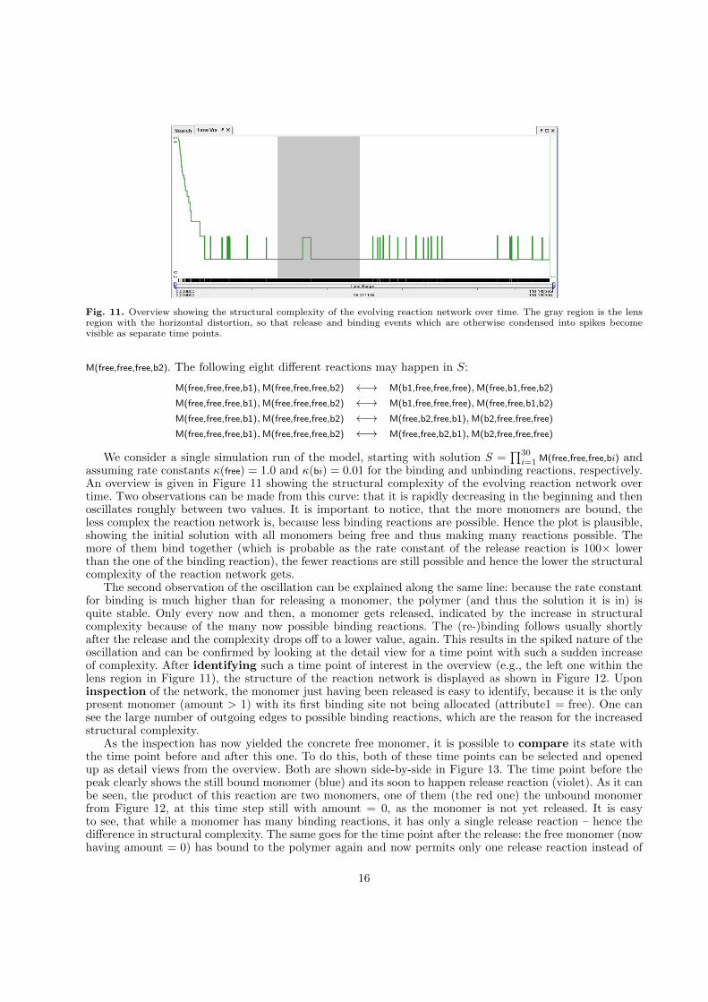
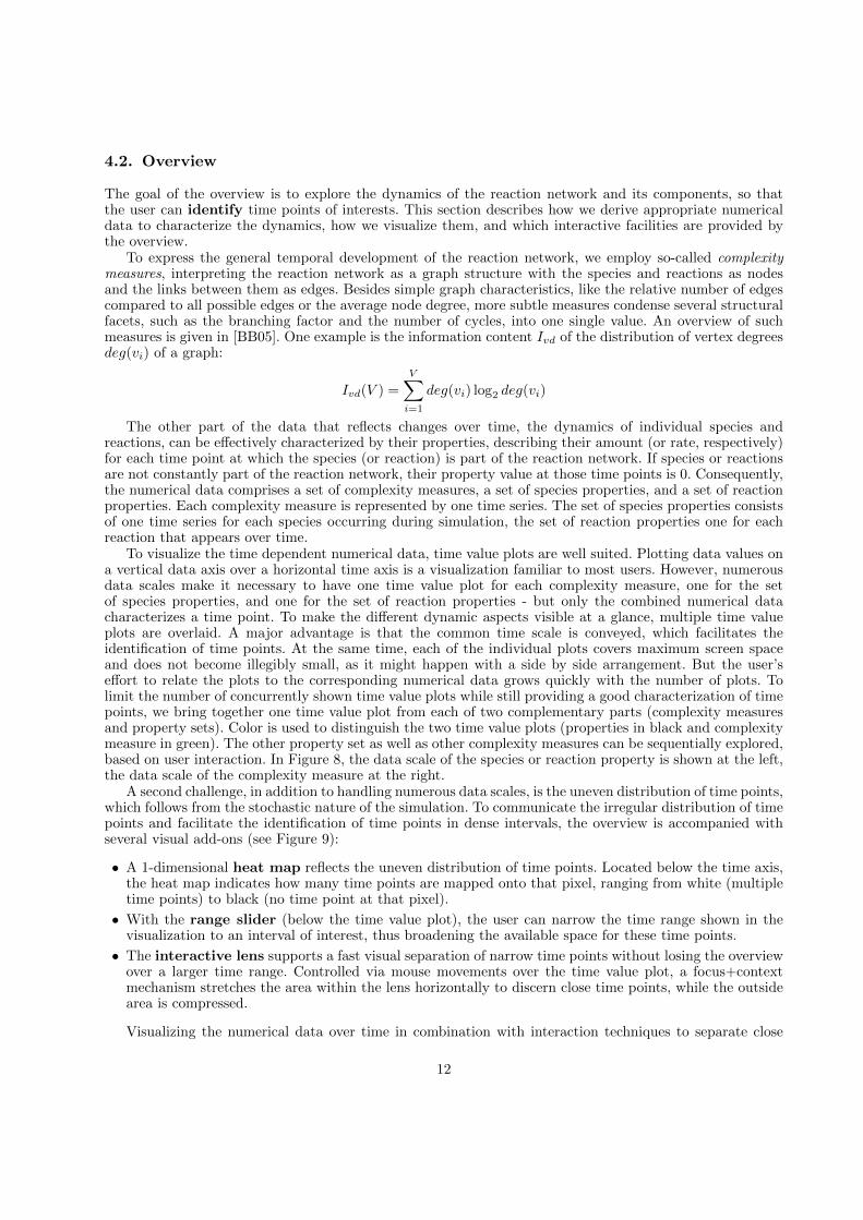
Fig. 11. Overview showing the structural complexity of the evolving reaction network over time. The gray region is the lensregion with the horizontal distortion, so that release and binding events which are otherwise condensed into spikes becomevisible as separate time points.

M(free,free,free,b2). The following eight different reactions may happen in S:

M(free,free,free,b1),M(free,free,free,b2) ←→ M(b1,free,free,free),M(free,b1,free,b2)

M(free,free,free,b1),M(free,free,free,b2) ←→ M(b1,free,free,free),M(free,free,b1,b2)

M(free,free,free,b1),M(free,free,free,b2) ←→ M(free,b2,free,b1),M(b2,free,free,free)

M(free,free,free,b1),M(free,free,free,b2) ←→ M(free,free,b2,b1),M(b2,free,free,free)

We consider a single simulation run of the model, starting with solution S =∏30i=1 M(free,free,free,bi) and

assuming rate constants κ(free) = 1.0 and κ(bi) = 0.01 for the binding and unbinding reactions, respectively.An overview is given in Figure 11 showing the structural complexity of the evolving reaction network overtime. Two observations can be made from this curve: that it is rapidly decreasing in the beginning and thenoscillates roughly between two values. It is important to notice, that the more monomers are bound, theless complex the reaction network is, because less binding reactions are possible. Hence the plot is plausible,showing the initial solution with all monomers being free and thus making many reactions possible. Themore of them bind together (which is probable as the rate constant of the release reaction is 100× lowerthan the one of the binding reaction), the fewer reactions are still possible and hence the lower the structuralcomplexity of the reaction network gets.

The second observation of the oscillation can be explained along the same line: because the rate constantfor binding is much higher than for releasing a monomer, the polymer (and thus the solution it is in) isquite stable. Only every now and then, a monomer gets released, indicated by the increase in structuralcomplexity because of the many now possible binding reactions. The (re-)binding follows usually shortlyafter the release and the complexity drops off to a lower value, again. This results in the spiked nature of theoscillation and can be confirmed by looking at the detail view for a time point with such a sudden increaseof complexity. After identifying such a time point of interest in the overview (e.g., the left one within thelens region in Figure 11), the structure of the reaction network is displayed as shown in Figure 12. Uponinspection of the network, the monomer just having been released is easy to identify, because it is the onlypresent monomer (amount > 1) with its first binding site not being allocated (attribute1 = free). One cansee the large number of outgoing edges to possible binding reactions, which are the reason for the increasedstructural complexity.

As the inspection has now yielded the concrete free monomer, it is possible to compare its state withthe time point before and after this one. To do this, both of these time points can be selected and openedup as detail views from the overview. Both are shown side-by-side in Figure 13. The time point before thepeak clearly shows the still bound monomer (blue) and its soon to happen release reaction (violet). As it canbe seen, the product of this reaction are two monomers, one of them (the red one) the unbound monomerfrom Figure 12, at this time step still with amount = 0, as the monomer is not yet released. It is easyto see, that while a monomer has many binding reactions, it has only a single release reaction – hence thedifference in structural complexity. The same goes for the time point after the release: the free monomer (nowhaving amount = 0) has bound to the polymer again and now permits only one release reaction instead of

16

Fig. 12. Detailed view showing the peak highlighted in Figure 11.

multiple binding reactions as before, effectively causing the drop-off in structural complexity. This confirmsthe assumption that alternating release and binding reactions cause the observed oscillatory pattern in thecomplexity plot.

4.5. Discussion

All in all, the presented method to visually explore dynamic biochemical reaction networks scales well to thesize as well as to the heterogeneous character of the data, with its structural and numerical facets. This isnoteworthy in the sense, that dynamic reaction networks can be interpreted as time-varying graphs, whichare notoriously hard to visualize, especially if it gets large and encompasses many time steps. Traditionally,in the area of Graph Drawing, the visualization of time-varying graphs is associated with the problem ofproviding a sequence of (stacked) views that maintain the mental model of the user. This means that agraph layout must be found that minimizes unnecessary positional changes across all time points in orderto ease comparison and traceability of the changes. Besides specifically tailored layout methods (e.g., theForesighted Layout with Tolerance [DG02]) also special visual metaphors (e.g., the Worm Metaphor [DE02])have been developed to cope with this challenge. Yet, these standard solutions do neither scale-up as muchas needed to cope with the amount of data produced in this scenario, nor are they able to allow the visualexploration of structural changes and changes in the node properties at the same time. This is, why awhole new visualization concept was needed, which copes with the possibly huge number of time steps bycondensing and plotting the structural information into complexity measures, and which deals with possiblylarge networks by utilizing a table-based visualization approach, which has been shown to scale up to about100,000 nodes [EK02]. By breaking the data down into its temporal and structural dimension and showingthese two facets in multiple linked views, the visual interface gives the user intuitive access to the complexdata. In this combination, the presented concept stands as a novel visualization solution in the area ofinteractive visualization.

5. Applicability to extensions of the π-calculus

Different extensions to the π-calculus for the stochastic modeling of cell-biological processes have beenproposed. spico [KLN07] associates sets of functions to channels. In [Kut06] an encoding from spico to thestochastic π-calculus is presented that only increases the amount of used channel names, thus yielding largerreaction sets. Since our approach is explicitly designed to deal with large reaction sets it is applicable tospico as well.

Other extensions cannot be translated back into the stochastic π-calculus. π@ [Ver07] and its stochasticversion Sπ@ [VB08] allow for communication on tuples of channels and thus increase the size of reaction setssimilar to spico. The attributed π-calculus [JLNU10] extends the idea of process parameters to molecule

17

Fig. 13. Detailed views showing the states of the reaction network before (top) and after (bottom) the peak from Figure 12.

attributes which can be of any type not just channels. Communication constraints are introduced that allowto make the rate of a communication dependent on the attribute values of interaction partners. To all ofthese extensions our approach can be well applied since it does not depend on how communication labelsare obtained and a biochemical form can be formulated for them in the same way as for the stochastic π-calculus, see e.g., [JLNU08]. In fact, our visualization is in particular designed for the attributed π-calculusconsidering molecules with attribute values. Notice that spico, π@, Sπ@, and also the attributed π-calculusallow for prioritized interactions.

BioAmbients [RPS+04], Brane Calculi [Car04], and BlenX [DPR08] associate locations with processes.This information may be integrated into our concept in two different ways. On one hand, one can try toreflect the location of processes as additional species attributes. In fact, the same idea is used for an encodingof BioAmbients into the attributed π-calculus, see [JLNU10]. On the other hand, spatial information couldalso be associated with reactions. Although the latter approach requires to extend the notion of reactionlabels accordingly, it does not impact the visualization since reaction nodes are considered to have propertieswhich are represented in the same way as the attributes of species nodes, see below. Yet, an extension of the

18

visualization that explicitly aims at the exploration of spatial information would be desirable in any casebut is subject to future work, see Section 6.

The imperative π-calculus [JLN09] extends on the attributed π-calculus by allowing processes to readand change values in a global imperative store. Effectively, this means that states are not entirely describedby processes but by pairs of processes and stores. In order to apply our approach to the imperative π-calculusboth the construction and the visualization of reaction networks needs to be extended. For the construction,communication and reaction labels need to capture possible effects on the global imperative store and theirrelations have to be adapted accordingly. These changes are then to be reflected in the components of thereaction network and the visualization.

6. Conclusion and Future Work

We conclude, that our two step approach of first constructing and then visualizing reaction networks fromthe states of stochastic π-calculus-models succeeds in bridging the gap between the notion of communicatingprocesses and models of biochemical systems. Furthermore, in our example, we observe that the synergyof formal and visual methods allows the modeler to gain additional confidence in the obtained results. Theclear formal definition of our transformation, its proof of correctness, and the fact the concepts defined in theformal step build the direct foundation of the visualization add to this point. The high interactivity of thepresented visualization concepts engages modelers more than a static plot and the combination of overviewand detail contributes to the overall understanding and detailed insights into the dynamics of biochemicalsystems.

In future work, we aim to provide even more direct ways of a back-and-forth transformation betweenabstract models and biochemical reaction networks. A first step in this direction has already been taken byproposing a new rule-based language [JLNV11], which can be shown to be as expressive as the π-calculus whileat the same time being much closer to the cell-biological domain. Another challenging aspect for visualizationas a whole, as well as our visualization concept in particular is the inclusion of multiple simulation runs.This would introduce another, even higher layer of overview, as the set of all simulation runs would rankabove the individual run shown in the overview so far. This is not only an issue in terms of screen real estate,but also in terms of providing linking and interaction between all different views. Lastly, the meaningfulinclusion and depiction of spatial information, i.e., compartments, beyond being just another table column,is of great interest for more advanced models involving transport processes, such as shuttling. In general,all these possible extensions of our visualization concept would enhance the exploration possibilities of thenetwork structures that result from stochastic simulation and thus broaden the application of our conceptto other domains.

Acknowledgements

The authors would like to thank Steffen Hadlak for his implementation work and Cedric Lhoussaine andJoachim Niehren for their valuable comments. This work was supported by the DFG Graduate School dIEMoSiRiS.

References

[BB05] Danail Bonchev and Gregory A. Buck. Quantitative measures of network complexity. In Danail Bonchev andDennis H. Rouvray, editors, Complexity in Chemistry, Biology, and Ecology, pages 191–235. Springer, 2005.

[Byr99] Donald Byrd. A scrollbar-based visualization for document navigation. In DL’99: Proceedings of the fourth ACMconference on Digital libraries, pages 122–129, 1999.

[Car04] Luca Cardelli. Brane Calculi - Interactions of Biological Membranes. In Computational Methods in SystemsBiology, International Conference, CMSB’04, LNCS, pages 257–278, 2004.

[Car08a] Luca Cardelli. From processes to ODEs by chemistry. In IFIP Theoretical Computer Science, pages 261–281, 2008.[Car08b] Luca Cardelli. On process rate semantics. Theoretical Computer Science, 391(3):190–215, 2008.[CCG+09] Luca Cardelli, Emmanuelle Caron, Philippa Gardner, Ozan Kahramanogullari, and Andrew Phillips. A Process

Model of Rho GTP-binding Proteins. Theoretical Computer Science, 410(33-34):3166–3185, 2009.[DE02] Tim Dwyer and Peter Eades. Visualising a fund manager flow graph with columns and worms. In IV’02: Proceedings

of the 6th International Conference on Information Visualisation, pages 147–152, 2002.

19

[DG02] Stephan Diehl and Carsten Gorg. Graphs, they are changing – dynamic graph drawing for a sequence of graphs.In GD’02: Proceedings of the 10th International Symposium on Graph Drawing, pages 23–31, 2002.

[DPR08] Lorenzo Dematte, Corrado Priami, and Alessandro Romanel. Modelling and Simulation of Biological Processes inBlenX. SIGMETRICS Performance Evaluation Review, 35(4):32–39, 2008.

[EK02] Stephen G. Eick and Alan F. Karr. Visual scalability. Journal of Computational and Graphical Statistics, 11(1):22–43, March 2002.

[FHR+03] James R. Faeder, William S. Hlavacek, Ilona Reischl, Michael L. Blinov, Henry Metzger, Antonio Redondo, CarlaWofsy, and Byron Goldstein. Investigation of early events in fcεri-mediated signaling using a detailed mathematicalmodel. Journal of Immunology, 170(7):3769–3781, 2003.

[Gil77] Daniel T. Gillespie. Exact stochastic simulation of coupled chemical reactions. The Journal of Physical Chemistry,81(25):2340–2361, 1977.

[HFB+03] William S. Hlavacek, James R. Faeder, Michael L. Blinov, Alan S. Perelson, and Byron Goldstein. The complexityof complexes in signal transduction. Biotechnology and Bioengineering, 84(7):783–794, 2003.

[JLN09] Mathias John, Cedric Lhoussaine, and Joachim Niehren. Dynamic compartments in the imperative pi-calculus.In Pierpaolo Degano and Roberto Gorrieri, editors, Computational Methods in Systems Biology, InternationalConference, CMSB’09, volume 5688 of Lecture Notes in Computer Sience, pages 235–250. Springer Verlag, 2009.

[JLNU08] Mathias John, Cedric Lhoussaine, Joachim Niehren, and Adelinde M. Uhrmacher. The attributed pi calculus. InComputational Methods in Systems Biology, International Conference, CMSB’08, volume 5307 of Lecture Notesin Computer Science, pages 83–102. Springer Verlag, 2008.

[JLNU10] Mathias John, Cedric Lhoussaine, Joachim Niehren, and Adelinde M. Uhrmacher. The attributed pi-calculuswith priorities. Transactions on Computaional Systems Biology XII. Special Issue on Modeling Methodologies,5945:13–76, February 2010. LNCS (Lecture Notes in Bioinformatics), Springer Berlin/Heidelberg.

[JLNV11] Mathias John, Cedric Lhoussaine, Joachim Niehren, and Cristian Versari. Biochemical reaction rules with con-straints. In Proceedings of the European Symposium on Programming, pages 338–357, 2011.

[KLN07] Celine Kuttler, Cedric Lhoussaine, and Joachim Niehren. A stochastic pi calculus for concurrent objects. InHirokazu Anai, Katsuhisa Horimoto, and Temur Kutsia, editors, Second International Conference on AlgebraicBiology, number 4545 in Lecture Notes in Computer Science, pages 232–246. Springer Verlag, 2007.

[Kut06] Celine Kuttler. Simulating bacterial transcription and translation in a stochastic pi-calculus. Transactions onComputational Systems Biology, 4220/2006:113–149, 2006.

[LJU10] Stefan Leye, Mathias John, and Adelinde M. Uhrmacher. A flexible architecture for performance experiments withthe pi-calculus and its extensions. In Barry Lawson, editor, 3rd International ICST Conference on SimulationTools and Techniques, ICST, Malaga, Spain. ICST/IEEE, 2010.

[MG09] Roland Meyer and Roberto Gorrieri. On the relationship between π-calculus and finite place/transition petrinets. In Mario Bravetti and Gianluigi Zavattaro, editors, CONCUR - Concurrency Theory, 20th InternationalConference, number 5710 in Lecture Notes in Computer Science, pages 463–480. Springer Verlag, 2009.

[Mil99] Robin Milner. Communicating and Mobile Systems: the π-calculus. Cambridge University Press, 1999.[MJM+09] Orianne Mazemondet, Mathias John, Carsten Maus, Adelinde M Uhrmacher, and Arndt Rolfs. Integrating diverse

reaction types into stochastic models - a signaling pathway case study in the imperative pi-calculus. In M. D.Rossetti, R. R. Hill, B. Johansson, A. Dunkin, and R. G. Ingalls, editors, Winter Simulation Conference, pages932–943. Institute of Electrical and Electronics Engineers, Inc., 2009.

[PC07] Andrew Phillips and Luca Cardelli. Efficient, correct simulation of biological processes in the stochastic pi-calculus.In Muffy Calder and Stephen Gilmore, editors, Computational Methods in Systems Biology, International Confer-ence, CMSB’07, volume 4695 of Lecture Notes in Computer Science, pages 184–199. Springer Verlag, 2007.

[PCC06] Andrew Phillips, Luca Cardelli, and Giuseppe Castagna. A graphical representation for biological processes in thestochastic pi-calculus. Transactions on Computational Systems Biology, 7:123–152, 2006.

[Phi] Andrew Phillips. Some 3D videos of SPiM simulations. http://research.microsoft.com/en-us/projects/spim/default.aspx. retrieved 05-OCT-2009.

[Pri95] Corrado Priami. Stochastic π-Calculus. Computer Journal, 6:578–589, 1995.[PRSS01] Corrado Priami, Aviv Regev, Ehud Y. Shapiro, and William Silverman. Application of a Stochastic Name-Passing

Calculus to Representation and Simulation of Molecular Processes. Information Processing Letters, 80(1):25–31,2001.

[RC94] Ramana Rao and Stuart K. Card. The table lens: Merging graphical and symbolic representations in an interac-tive focus+context visualization for tabular information. In ACM SIGCHI’94: Proceedings of the ACM SIGCHIConference on Human Factors in Computing Systems, pages 111–117, 1994.

[Reg03] Aviv Regev. Computational Systems Biology: A Calculus for Biomolecular Knowledge. PhD thesis, Tel AvivUniversity, 2003.

[RPS+04] Aviv Regev, Ekaterina M. Panina, William Silverman, Luca Cardelli, and Ehud Shapiro. BioAmbients: An Ab-straction for Biological Compartments. Theoretical Computer Science, 325(1):141–167, 2004.

[SJUS08] Hans-Jorg Schulz, Mathias John, Andrea Unger, and Heidrun Schumann. Visual analysis of bipartite biologicalnetworks. In VCBM’08: Proceedings of the Eurographics Workshop on Visual Computing for Biomedicine, pages135–142, 2008.

[TAS09] Christian Tominski, James Abello, and Heidrun Schumann. CGV – an interactive graph visualization system.Computers and Graphics, 33(6):660–678, December 2009.

[TK08] Oksana Tymchyshyn and Marta Z. Kwiatkowska. Combining Intra- and Inter-cellular Dynamics to InvestigateIntestinal Homeostasis. In Formal Methods in Systems Biology, First International Workshop, FMSB 2008, pages63–76, 2008.

20

[VB08] Cristian Versari and Nadia Busi. Efficient stochastic simulation of biological systems with multiple variable volumes.Electronic Notes in Theoretical Computer Science, 194(3):165–180, 2008.

[Ver07] Cristian Versari. A core calculus for a comparative analysis of bio-inspired calculi. In European Symposium onProgramming (ESOP’07), pages 411–425, 2007.

21