HAL Id: hal-00836413https://hal.inria.fr/hal-00836413

Submitted on 20 Jun 2013

HAL is a multi-disciplinary open accessarchive for the deposit and dissemination of sci-entific research documents, whether they are pub-lished or not. The documents may come fromteaching and research institutions in France orabroad, or from public or private research centers.

L’archive ouverte pluridisciplinaire HAL, estdestinée au dépôt et à la diffusion de documentsscientifiques de niveau recherche, publiés ou non,émanant des établissements d’enseignement et derecherche français ou étrangers, des laboratoirespublics ou privés.

Constructing analysis-suitable parameterization ofcomputational domain from CAD boundary by

variational harmonic methodGang Xu, Bernard Mourrain, Régis Duvigneau, André Galligo

To cite this version:Gang Xu, Bernard Mourrain, Régis Duvigneau, André Galligo. Constructing analysis-suitable param-eterization of computational domain from CAD boundary by variational harmonic method. Journal ofComputational Physics, Elsevier, 2013, 252, pp.275-289. 10.1016/j.jcp.2013.06.029. hal-00836413

Constructing analysis-suitable parameterization of computational domain

from CAD boundary by variational harmonic method

Gang Xua,b,∗, Bernard Mourrainb, Regis Duvigneauc, Andre Galligod

aCollege of Computer Science, Hangzhou Dianzi University, Hangzhou 310018, P.R.ChinabGalaad, INRIA Sophia-Antipolis, 2004 Route des Lucioles, 06902 Cedex, FrancecOPALE, INRIA Sophia-Antipolis, 2004 Route des Lucioles, 06902 Cedex, France

dUniversity of Nice Sophia-Antipolis, 06108 Nice Cedex 02, France

Abstract

In isogeometric analysis, parameterization of computational domain has great effects as mesh

generation in finite element analysis. In this paper, based on the concept of harmonic mapping

from the computational domain to parametric domain, a variational harmonic approach is proposed

to construct analysis-suitable parameterization of computational domain from CAD boundary for

2D and 3D isogeometric applications. Different from the previous elliptic mesh generation method

in finite element analysis, the proposed method focus on isogeometric version, and converts the

elliptic PDE into a nonlinear optimization problem, in which a regular term is integrated into the

optimization formulation to achieve more uniform and orthogonal iso-parametric structure near

convex (concave) parts of the boundary. Several examples are presented to show the efficiency of

the proposed method in 2D and 3D isogeometric analysis.

Keywords: isogeometric analysis; grid generation; harmonic mapping; variational method ;

analysis-suitable parameterization

∗Corresponding author.Email addresses: xugangzju@gmail.com; gxu@hdu.edu.cn (Gang Xu ), Bernard.Mourrain@inria.fr (Bernard

Mourrain), Regis.Duvigneau@inria.fr (Regis Duvigneau), galligo@unice.fr (Andre Galligo)

Preprint submitted to Journal of Computational Physics June 10, 2013

1. Introduction

The isogeometric analysis (IGA for short) method proposed by Hughes et al. in [19] is a

new computational approach that offers the possibility of seamless integration between CAD and

CAE. The method uses the same type of mathematical representation (spline representation),

both for the geometry and for the physical solutions, and thus avoids this costly forth and back

transformations. Moreover its reduces the number of parameters needed to describe the geometry,

which is of particular interest for shape optimization.

Mesh generation, which generates a discrete grid of a computational domain from a given CAD

object, is a key and the most time-consuming step in finite element analysis (FEA for short). It

consumes about 80% of the overall design and analysis process [6] in aerospace, automotive and

ship industry. Parametrization of computational domain in IGA, which corresponds to the mesh

generation in FEA, also has some impact on analysis result and efficiency. In particular, arbitrary

refinements can be performed on the computational mesh in FEA, but in IGA if we compute with

tensor product B-splines, we can only perform refinement operations in each parametric direction

by knot insertion or degree elevation. Hence, parameterization of computational domain is also

being important for IGA. As it is pointed by Cottrell et al. [9], one of the most significant challenges

towards isogeometric analysis is constructing analysis-suitable parameterizations from given CAD

boundary representation.

Parameterization of a computational domain in IGA is determined by control points, knot

vectors and the degrees of B-spline objects. For 2D and 3D IGA problems, the knot vectors and

the degree of the computational domain are determined by the given boundary curves/surfaces.

That is, given boundary curves/surfaces, the quality of parameterization of computational domain

is determined by the positions of inner control points. Hence, finding a good placement of the inner

control points inside the computational domain, is a key issue. As the required mesh quality in

FEA [28, 29, 30], a basic requirement of the resulting parameterization for IGA is that it doesn’t

have self-intersections, so that it is an injective map from the parametrization domain to the

computational domain.

In the field of mesh generation in FEA, a general method is based on partial differential

equations [27]. The grid points are the solution of an elliptic partial differential equation system

with Dirichlet boundary conditions on all boundaries. There are several advantages in elliptic

2

mesh generation. The theory of partial differential equations guarantees that the mapping between

physical and transformed regions will be one-to-one. Another important property is the inherent

smoothness in the solution of elliptic systems. A disadvantage of elliptic method is that there will

be some non-uniform grid elements near convex (concave) parts of the boundary. Moreover, special

treatment should be considered to achieve orthogonal mesh [32, 41, 40].

Motivated from the elliptic grid generation method in FEA, in this paper, we study the analysis-

suitable parameterization problem of computational domain in isogeometric analysis. Our main

contributions are:

• A nonlinear optimization framework based on harmonic mapping theory is proposed to gen-

erate a analysis-suitable parameterization of computational domain without self-intersections

for 2D and 3D isogeometric applications.

• A regular term is integrated into the optimization formulation to achieve more uniform and

orthogonal iso-parametric structure near convex (concave) parts of the boundary.

• We test the parameterization results on 2D and 3D heat conduction problems to show the

effectiveness of the proposed method.

The rest of the paper is organized as follows. Section 2 reviews the related work in IGA.

Section 3 describes the variational harmonic method for analysis-suitable parameterization of 2D

computational domain. The 3D case for volume parameterization is studied in Section 4. Some

examples and comparisons based on the isogeometric heat conduction problem are presented in

Section 5. Finally, we conclude this paper and outline future works in Section 6.

2. Related work

In this section, we will review some related works in IGA and parameterization of computational

domains.

IGA was firstly proposed by Hughes et al. [19] in 2005 to achieve the seamless integration

of CAD and FEA. Since then, many researchers in the fields of computational mechanical and

geometric computation were involved in this topic. The current work on isogeometric analysis

can be classified into four categories: (1) application of IGA to various simulation problems [3,

5, 11, 18, 12, 26]; (2) application of various modeling tools such as T-splines and PHT-splines in

3

CAGD to IGA [6, 7, 13, 23, 24]; (3) accuracy and efficiency improvement of IGA framework by

reparameterization and refinement operations [1, 4, 8, 10, 35, 36]; (4) construction of analysis-

suitable computational domain from boundary information [1, 21, 22, 31, 36, 37, 38, 39].

The topic of this paper belongs to the forth field. From the viewpoint of graphics applications,

volume parameterization of 3D models has been studied in [20, 34, 33]. As far as we know, there

are only a few work on the parametrization of computational domains from the viewpoint of

isogeometric applications. Martin et al. [21] proposed a method to fit a genus-0 triangular mesh

by B-spline volume parameterization, based on discrete volumetric harmonic functions; this can be

used to build computational domains for 3D IGA problems. A variational approach for constructing

NURBS parameterization of swept volumes is proposed by Aigner et al [1]. Many free-form shapes

in CAD systems, such as blades of turbines and propellers, are covered by this kind of volumes.

Cohen et.al. [8] proposed the concept of analysis-aware modeling, in which the parameters of CAD

models should be selected to facilitate isogeometric analysis. They also demonstrated the influence

of parameterization of computational domains by several examples. Escobar et al. proposed

a method to construct a trivariate T-spline volume of complex genus-zero solids for isogeometric

application by using an adaptive tetrahedral meshing and mesh untangling technique [15]. However,

the obtained solid T-splines have elements with negative Jacobians at the Gauss quadrature points.

Zhang et al. proposed a robust and efficient algorithm to construct injective solid T-splines for

genus-zero geometry from a boundary triangulation [38]. Based on the Morse theory, a volumetric

parameterization method of mesh model with arbitrary topology is proposed in [31]. The above

proposed methods demand a surface triangulation as input data. For the CAD boundary with

spline representation, r-refinement method for generating optimal analysis-aware parameterization

of computational domain is proposed based on shape optimization method [35, 36]. However, it only

works for specified analysis problems. In [37], a constraint optimization framework is proposed to

obtain analysis-suitable volume parameterization of computational domain. Pettersen and Skytt

proposed the spline volume faring method to obtain high-quality volume parameterization for

isogeometric applications [25]. Zhang et al. studied the construction of conformal solid T-spline

from boundary T-spline representation by octree structure and boundary offset [39]. In this paper,

based on the harmonic mapping theory, we propose a general method to construct analysis-suitable

parameterization of computational domain from given CAD boundary information.

4

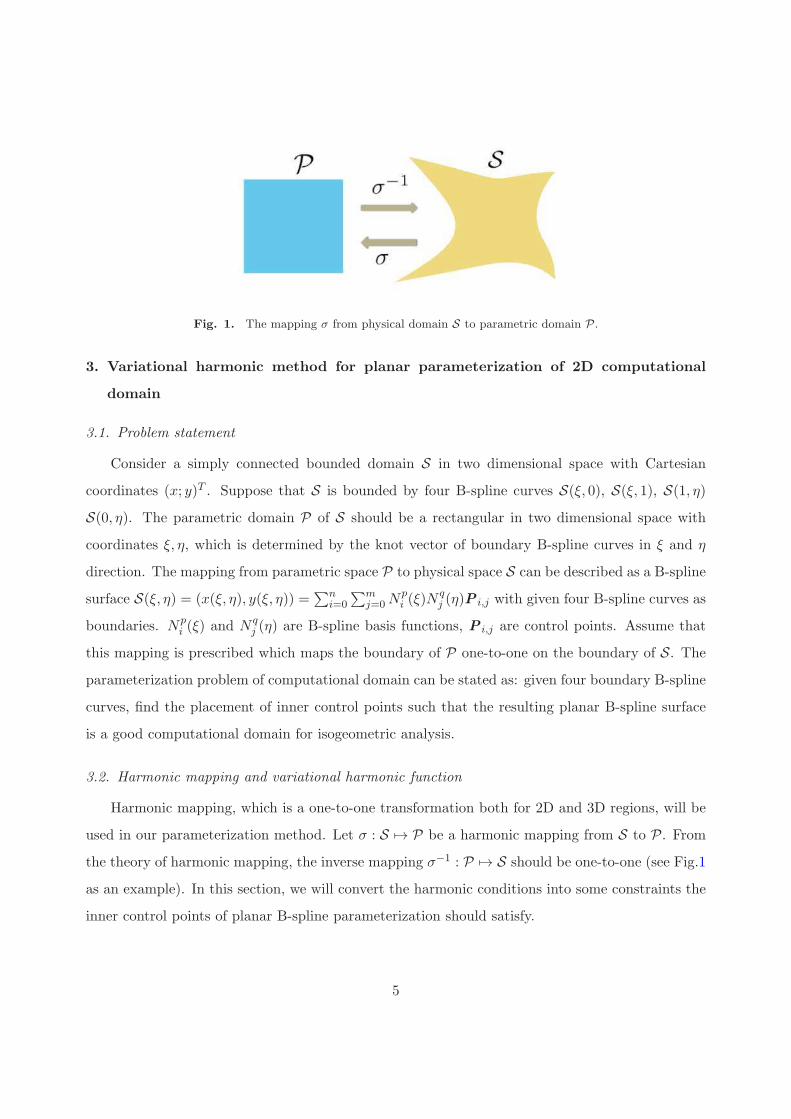
Fig. 1. The mapping σ from physical domain S to parametric domain P.

3. Variational harmonic method for planar parameterization of 2D computational

domain

3.1. Problem statement

Consider a simply connected bounded domain S in two dimensional space with Cartesian

coordinates (x; y)T . Suppose that S is bounded by four B-spline curves S(ξ, 0), S(ξ, 1), S(1, η)

S(0, η). The parametric domain P of S should be a rectangular in two dimensional space with

coordinates ξ, η, which is determined by the knot vector of boundary B-spline curves in ξ and η

direction. The mapping from parametric space P to physical space S can be described as a B-spline

surface S(ξ, η) = (x(ξ, η), y(ξ, η)) =∑n

i=0

∑mj=0N

pi (ξ)N

qj (η)P i,j with given four B-spline curves as

boundaries. Npi (ξ) and N q

j (η) are B-spline basis functions, P i,j are control points. Assume that

this mapping is prescribed which maps the boundary of P one-to-one on the boundary of S. The

parameterization problem of computational domain can be stated as: given four boundary B-spline

curves, find the placement of inner control points such that the resulting planar B-spline surface

is a good computational domain for isogeometric analysis.

3.2. Harmonic mapping and variational harmonic function

Harmonic mapping, which is a one-to-one transformation both for 2D and 3D regions, will be

used in our parameterization method. Let σ : S 7→ P be a harmonic mapping from S to P. From

the theory of harmonic mapping, the inverse mapping σ−1 : P 7→ S should be one-to-one (see Fig.1

as an example). In this section, we will convert the harmonic conditions into some constraints the

inner control points of planar B-spline parameterization should satisfy.

5

Suppose that σ : S 7→ P is a harmonic mapping, that is

∆ξ(x, y) = ξxx + ξyy = 0

∆η(x, y) = ηxx + ηyy = 0

By chain rules, we have

dξ = ξxdx+ ξydy = ξx(xξdξ + xηdη) + ξy(yξdξ + yηdη)

dη = ηxdx+ ηydy = ηx(xξdξ + xηdη) + ηy(yξdξ + yηdη)

From above two equation, we have

ξxxξ + ξyyξ = ηxxη + ηyyη = 1 (1)

ξxxη + ξyyη = ηxxξ + ηyyξ = 0 (2)

By solving above two linear systems, we obtain

ξx =yηJ, ξy =

−xηJ

, ηx =−yξJ

, ηy =xξJ

where

J = xξyη − xηyξ

is Jacobian of transformation from P to S.

From above results and ∂∂x

= ξx∂∂ξ, ∂∂y

= ξy∂∂ξ

, we have

J∆ξ(x, y) = J∂

∂xξx + J

∂

∂yξy

= (Jξx∂

∂ξ+ Jηx

∂

∂η)ξx + (Jξy

∂

∂ξ+ Jηy

∂

∂η)ξy

= (yη∂

∂ξ− yξ

∂

∂η)(yξJ) + (−xη

∂

∂ξ+ xξ

∂

∂η)(−xηJ

) = 0

After differential computation, we have

−yηLx+ xηLy = 0

where

L = (x2η + y2η)∂2

∂ξ2− 2(xξxη + yξyη)

∂2

∂ξη+ (x2ξ + y2ξ )

∂2

∂η2

6

Similarly, from J∆η(x, y) = 0, we have

yξLx− xξLy = 0

Then we obtain

Lx(ξ, η) = Ly(ξ, η) = 0

that is,

‖ LS(ξ, η) ‖2= (Lx)2 + (Ly)2 = 0

This is a nonlinear system in terms of inner control points of the planar B-spline parameterization.

The final grid obtained by this method usually has non-uniform elements near convex (concave)

boundary region. In order to solve this problem, we minimize the following energy function, which

is related to the uniformity of the iso-parametric net on the B-spline surface,∫∫

‖ Sξξ ‖2 + ‖ Sηη ‖2 +2 ‖ Sξη ‖2 dξdη.

Moreover, orthogonality is also an important property for analysis-suitable parameterization

in numerical simulation [40, 32]. In order to achieve an iso-parametric structure with good orthog-

onality, we minimize the following energy function as in [36]∫∫

‖ Sξ ‖2 + ‖ Sη ‖2 dξdη.

Then by adding the harmonic mapping term into above two energy functions, we obtain a new

energy function for parameterization of computational domain∫∫

‖ LS(ξ, η) ‖2 +λ1(‖ Sξξ ‖2 + ‖ Sηη ‖2

+2 ‖ Sξη ‖2) + λ2(‖ Sξ ‖2 + ‖ Sη ‖2)dξdη (3)

where λ1 and λ2 are positive weights to control the final parameterization results.

Remark 3.1. For different choice of λ1 and λ2 in the objective function (3), different parameter-

ization results will be achieved. If λ1 > λ2, then the resulting iso-parametric structure has better

uniformity. If λ2 > λ1, then we can obtain an iso-parametric grid with better orthogonality. See

Fig.3 for an example to show the effects of the positive weights λ1 and λ2.

The Discrete Coons method is used to construct initial inner control points, and the Steepest

Descent method is employed to minimize the energy function. The details will be described in the

following two subsections.

7

(a) (b)

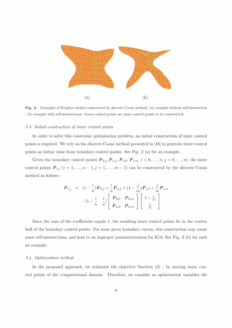
Fig. 2. Examples of B-spline surface constructed by discrete Coons method: (a) example without self-intersection

; (b) example with self-intersections. Green control points are inner control points to be constructed.

3.3. Initial construction of inner control points

In order to solve this constraint optimization problem, an initial construction of inner control

points is required. We rely on the discrete Coons method presented in [16] to generate inner control

points as initial value from boundary control points. See Fig. 2 (a) for an example.

Given the boundary control points P0,j ,Pn,j ,P i,0, P i,m, i = 0, . . . , n, j = 0, . . . ,m, the inner

control points P i,j (i = 1, . . . , n − 1, j = 1, . . . ,m − 1) can be constructed by the discrete Coons

method as follows:

P i,j = (1−i

n)P0,j +

i

nPn,j + (1−

j

m)P i,0 +

j

mP i,m

−[1−i

n

i

n]

P0,0 P0,m

Pn,0 Pn,m

1− jm

jm

Since the sum of the coefficients equals 1, the resulting inner control points lie in the convex

hull of the boundary control points. For some given boundary curves, this construction may cause

some self-intersections, and lead to an improper parameterization for IGA. See Fig. 2 (b) for such

an example.

3.4. Optimization method

In the proposed approach, we minimize the objective function (3) , by moving inner con-

trol points of the computational domain. Therefore, we consider as optimization variables the

8

coordinates of the inner control points and as cost function the error of the IGA solution. The op-

timization algorithm used for this study is a classical steepest-descent method in conjunction with

a back-tracking line-search. For this exercise, the gradient of the cost function is approximated

using a centered finite-differencing scheme.

Each iteration k of the optimization algorithm can be summarized as follows, starting from a

point xk in the variable space:

1. Evaluation of perturbed points xk + ǫek

2. Estimation of the gradient ∇f(xk) by finite-difference

3. Define search direction dk = −∇f(xk)

4. Line search : find ρ such as f(xk + ρdk) < f(xk)

These steps are carried out until a stopping criterion is satisfied.

3.5. Overview of variational harmonic method

In general, the proposed variational harmonic method can be summarized as follows:

Input: four coplanar boundary B-spline curves

Output: inner control points and the corresponding planar B-spline surfaces

• Construct the initial inner control points by discrete Coons method as in subsection 3.3;

• Solve the following optimization problem by using steepest-descent method

Min

∫∫

‖ LS(ξ, η) ‖2 +λ1(‖ Sξξ ‖2 + ‖ Sηη ‖2

+2 ‖ Sξη ‖2) + λ2(‖ Sξ ‖2 + ‖ Sη ‖2)dξdη

• Generate the corresponding planar B-spline surface S(ξ, η) as computational domain.

4. Variational harmonic method for volume parameterization of 3D computational

domain

In this section, we will study the volume parameterization problem by variational harmonic

method. Suppose that S is a simply connected bounded domain in three dimensional space

with Cartesian coordinates (x; y; z)T , and is bounded by six B-spline surfaces S(ξ, 0, ζ),S(ξ, 1, ζ),

9

S(1, η, ζ),S(0, η, ζ), S(ξ, η, 0),S(ξ, η, 1). The parametric domain P of S should be a cube in three

dimensional space with coordinates ξ, η, ζ, which is determined by the knot vector of boundary

B-spline surfaces in ξ, η and ζ direction. The mapping from parametric space P to physi-

cal space S can be described as a B-spline volume S(ξ, η, ζ) = (x(ξ, η, ζ), y(ξ, η, ζ), z(ξ, η, ζ)) =∑n

i=0

∑mj=0

∑lk=0N

pi (ξ) N q

j (η)Nrk (ζ)P i,j,k with given six B-spline surfaces as boundaries. Np

i (ξ),

N qj (η) and N r

k (ζ) are B-spline basis functions, P i,j,k are control points. Assume that this map-

ping is prescribed which maps the boundary of P one-to-one on the boundary of S. The volume

parameterization problem of 3D computational domain can be stated as: given six boundary B-

spline surfaces, find the placement of inner control points such that the resulting trivariate B-spline

parametric volume is a good computational domain for 3D isogeometric analysis.

4.1. Harmonic mapping and variational harmonic function

Similar with the 2D case, the harmonic conditions in 3D case will be converted into some

constraints the inner control points of trivariate B-spline volume parameterization should satisfy.

If the mapping σ : S 7→ P is a harmonic mapping, we have

∆ξ(x, y, z) = ξxx + ξyy + ξzz = 0

∆η(x, y, z) = ηxx + ηyy + ηzz = 0

∆ζ(x, y, z) = ζxx + ζyy + ζzz = 0

By chain rules, we have

dξ = ξxdx+ ξydy + ξzdz = ξx(xξdξ + xηdη + xζdζ)

+ξy(yξdξ + yηdη + yζdζ) + ξz(zξdξ + zηdη + zζdζ)

dη = ηxdx+ ηydy + ηzdz = ηx(xξdξ + xηdη + xζdζ)

+ηy(yξdξ + yηdη + yζdζ) + ηz(zξdξ + zηdη + zζdζ)

dζ = ζxdx+ ζydy + ζzdz = ζx(xξdξ + xηdη + xζdζ)

+ζy(yξdξ + yηdη + yζdζ) + ζz(zξdξ + zηdη + zζdζ)

10

From above three equation, we have

ξxxξ + ξyyξ + ξzzξ = 1

ηxxη + ηyyη + ηzzη = ζxxζ + ζyyζ + ζzzζ = 1

ξxxη + ξyyη + ξzzη = ηxxξ + ηyyξ + ηzzξ = 0

ξxxζ + ξyyζ + ξzzζ = ζxxξ + ζyyξ + ζzzξ = 0

ηxxζ + ηyyζ + ηzzζ = ζxxη + ζyyη + ζzzη = 0

By solving above three linear systems, we obtain

ξx =yηzζ − yζzη

J, ξy = −

xηzζ − xζzηJ

, ξz =yηzζ − yζzη

J,

ηx =yξzζ − yζzξ

J, ηy = −

xξzζ − xζzξJ

, ηz =yξzζ − yζzξ

J,

ζx =yηzξ − yξzη

J, ζy = −

xηzξ − xξzηJ

, ζz =yηzξ − yξzη

J,

where

J =

∣

∣

∣

∣

∣

∣

∣

∣

∣

xξ yξ zξ

xη yη zη

xζ yζ zζ

∣

∣

∣

∣

∣

∣

∣

∣

∣

is Jacobian of transformation from P to S.

From above results and J∆ξ(x, y, z) = 0,J∆η(x, y, z) = 0, J∆ζ(x, y, z) = 0, the following

condition can be derived,

Lx(ξ, η, ζ) = Ly(ξ, η, ζ) = Lz(ξ, η, ζ) = 0 (4)

where

L = a11∂2

∂ξ2+ 2a12

∂2

∂ξη+ 2a13

∂2

∂ξζ+ a22

∂2

∂η2+ 2a23

∂2

∂ηζ+ a33

∂2

∂ζ2,

a11 = a22a33 − a223, a12 = a13a23 − a12a33, a

13 = a12a23 − a13a22,

a22 = a11a33 − a213, a23 = a13a12 − a11a23, a

33 = a11a22 − a212,

and

a11 = (Sξ,Sξ), a12 = (Sξ,Sη), a13 = (Sξ,Sζ),

a22 = (Sη,Sη), a23 = (Sη,Sζ), a33 = (Sζ ,Sζ).

11

Eq. (4) can be rewritten as

‖ LS(ξ, η, ζ) ‖2= (Lx)2 + (Ly)2 + (Lz)2 = 0

Similarly with the 2D problem, it is also a nonlinear system in terms of inner control points of

the B-spline volume. In order to achieve uniform and orthogonal iso-parametric structure near

convex(concave) boundary region, we minimize the following energy function as in [37]

∫∫

λ1(‖ Sξξ ‖2 + ‖ Sηη ‖2 + ‖ Sζζ ‖

2 +2 ‖ Sξη ‖2 +2 ‖ Sηζ ‖2 +2 ‖ Sξζ ‖

2)

+λ2(‖ Sξ ‖2 + ‖ Sη ‖2 + ‖ Sζ ‖

2)dξdηdζ,

in which the first part with coefficient λ1 is related to the uniformity of the iso-parametric struc-

ture, and the second part with coefficient λ2 is related to the orthogonality of the iso-parametric

structure.

A new energy function for volume parameterization of computational domain can be obtained

by combining the harmonic mapping term and the above energy function as follows,

∫∫

‖ LS(ξ, η, ζ) ‖2 +λ1(‖ Sξξ ‖2 + ‖ Sηη ‖2 + ‖ Sζζ ‖

2

+2 ‖ Sξη ‖2 +2 ‖ Sηζ ‖2 +2 ‖ Sξζ ‖

2)

+λ2(‖ Sξ ‖2 + ‖ Sη ‖2 + ‖ Sζ ‖

2)dξdηdζ (5)

where λ1 and λ2 are positive weights to control the final parameterization results.

Remark 4.1. The weights λ1 and λ2 have similar effects on the volume parameterization results

as stated in Remark 3.1.

4.2. Initial construction of inner control points

The initial construction of inner control points for volume parameterization is based on the

discrete Coons volume generation method [35], which can be considered as the trivariate general-

ization of the discrete Conns patches presented in [16].

Suppose that the given boundary surfaces are B-spline surfaces and that the opposite boundary

B-spline surfaces have the same degree, number of control points and knot vectors. The interior

control points P i,j,k can be constructed as linear combination of boundary control points according

to the following formulas:

12

P i,j,k = (1− i/l)P0,j,k + i/lP l,j,k + (1− j/m)P i,0,k

+j/mP i,m,k + (1− k/n)P i,j,0 + k/nP i,j,n

−[1− i/l, i/l]

P0,0,k P0,m,k

P l,0,k P l,m,k

1− j/m

j/m

−[1− j/m, j/m]

P i,0,0 P i,0,n

P i,m,0 P i,m,n

1− k/n

k/n

−[1− k/n, k/n]

P0,j,0 P l,j,0

P0,j,n P l,j,n

1− i/l

i/l

+(1− k/n)

[1− i/l, i/l]

P0,0,0 P0,m,0

P l,0,0 P l,m,0

1− j/m

j/m

+k/n

[1− i/l, i/l]

P0,0,n P0,m,n

P l,0,n P l,m,n

1− j/m

j/m

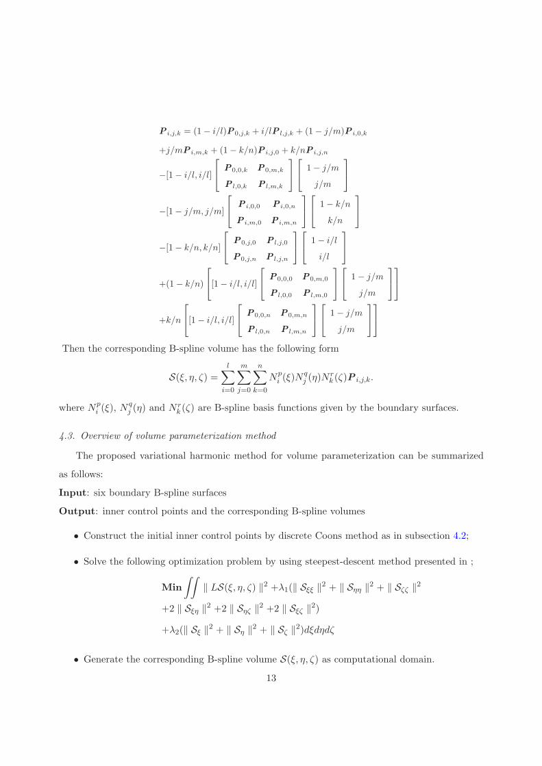
Then the corresponding B-spline volume has the following form

S(ξ, η, ζ) =l

∑

i=0

m∑

j=0

n∑

k=0

Npi (ξ)N

qj (η)N

rk (ζ)P i,j,k.

where Npi (ξ), N

qj (η) and N r

k (ζ) are B-spline basis functions given by the boundary surfaces.

4.3. Overview of volume parameterization method

The proposed variational harmonic method for volume parameterization can be summarized

as follows:

Input: six boundary B-spline surfaces

Output: inner control points and the corresponding B-spline volumes

• Construct the initial inner control points by discrete Coons method as in subsection 4.2;

• Solve the following optimization problem by using steepest-descent method presented in ;

Min

∫∫

‖ LS(ξ, η, ζ) ‖2 +λ1(‖ Sξξ ‖2 + ‖ Sηη ‖2 + ‖ Sζζ ‖

2

+2 ‖ Sξη ‖2 +2 ‖ Sηζ ‖2 +2 ‖ Sξζ ‖

2)

+λ2(‖ Sξ ‖2 + ‖ Sη ‖2 + ‖ Sζ ‖

2)dξdηdζ

• Generate the corresponding B-spline volume S(ξ, η, ζ) as computational domain.

13

5. Examples and comparison

In this section, we aim at presenting several examples to show the efficiency of the proposed

method. We will also give a comparison study between the original parameterization and the final

parameterization constructed by the proposed method based on the 2D and 3D heat conduction

problem.

5.1. Test model — heat conduction problem

For ease of presentation, we consider the second order elliptic PDE with homogeneous Dirichlet

boundary condition as an illustrative model problem :

−∆U(x) = f(x) in Ω

U(x) = 0 on ∂Ω(6)

where x are the Cartesian coordinates, Ω is a Lipschitz domain with boundary ∂Ω, f(x) ∈ L2(Ω) :

Ω 7→ R is a given source term, and U(x) : Ω 7→ R is the unknown solution.

Starting from a planar B-spline surface (or trivariate B-spline parametric volume) as compu-

tational domain, a general framework of an isogeometric solver for 2D and 3D heat conduction

problem (6) has been implemented as a plugin in the AXEL1 platform, yielding a B-spline surface

(or B-spline volume) as solution field. Additional details concerning the isogeometric solver of

problem (6) can be found in [14]. The proposed variational harmonic method is implemented as a

part of the isogeometric toolbox of the project EXCITING2.

In this paper, we test the different parameterizations of computational domains for 2D heat

conduction problem (6) with source term

f (x, y) =4π2

9sin(

πx

3) sin(

πy

3).

and 3D problem with source term

f (x, y, z) =π2

3sin(

πx

3) sin(

πy

3) sin(

πz

3).

For problems with unknown exact solution U , suppose that Uh is the approximation solution

obtained by isogeometric method, then the discrete error e = U−Uh. We employ a posteriori error

1http://axel.inria.fr/2http://exciting-project.eu/

14

assessment proposed in [36] to compare the initial and final parameterization of the computational

domain. It can be obtained by resolving the following problem,

∆e = −f +∆Uh in Ω (7)

e = 0 on ∂ΩD

The approximation error e from (7) also has a B-spline form. Some h-refinement operation

should be performed to achieve more accurate results for above problem. Though it is much more

expensive, it can be used as an error assessment method to show the effectiveness of the proposed

construction method of computational domain.

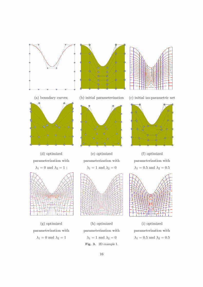
The first 2D example is shown in Fig. 3. Fig. 3 (a) presents the given boundary B-spline curves.

Fig. 3(b) presents the initial parametrization of computational domain constructed by discrete

Coons method. Fig. 3(c) shows the iso-parametric curves of the initial B-spline parameterization.

Fig. 3(d), Fig. 3 (e) and Fig. 3(f) show the optimized parametrization of computational domain

constructed by the proposed variational harmonic method with different choice of λ1 and λ2. The

corresponding iso-parametric structure of the resulting planar B-spline parameterization are shown

in Fig. 3(g), Fig. 3 (h) and Fig. 3(i) respectively. As described in Remark 3.1, the iso-parametric

structure with λ1 = 0 and λ2 = 1 in Fig. 3(g) has the best orthogonality, the iso-parametric net

with λ1 = 1 and λ2 = 0 in Fig. 3(h) has the best uniformity, and a good balance between uniformity

and orthogonality can be achieved in Fig. 3(i) with λ1 = 0.5 and λ2 = 0.5. The corresponding

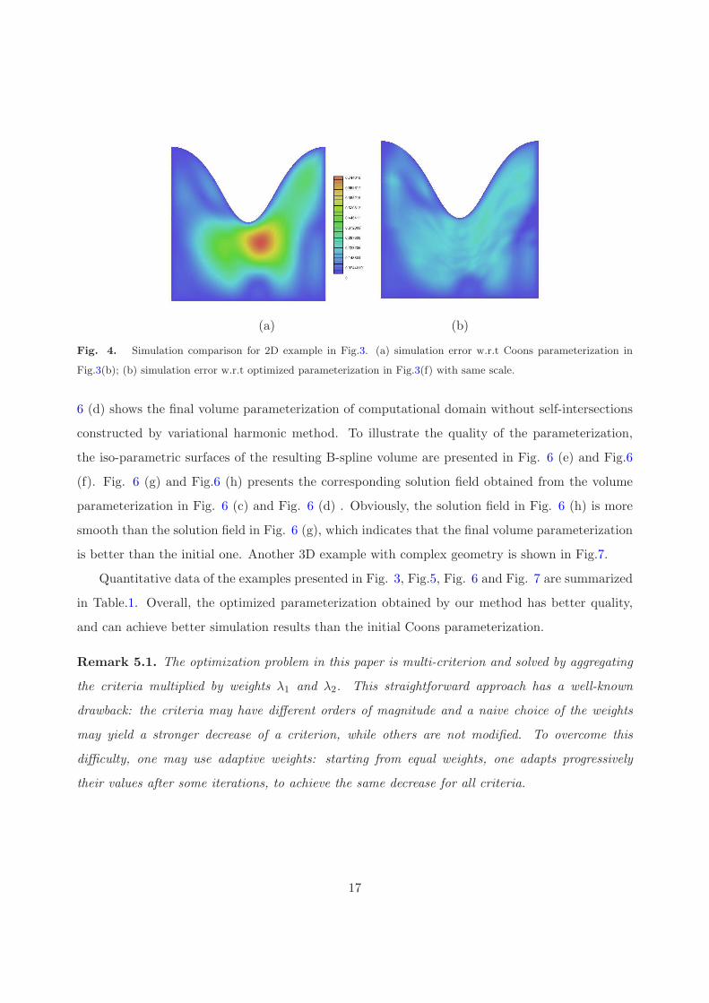
simulation errors of 2D heat conduction problem (7) for different parameterization shown in Fig.

3(b) and Fig. 3(f) are illustrated in Fig. 4 (a) and Fig. 4 (b) with the same scale.

Another 2D example is illustrated in Fig. 5. The given boundary B-spline curves is shown in

Fig. 5 (a). Fig. 5(b) presents the initial parametrization of computational domain constructed by

discrete Coons method. There are some self-intersections on the initial parameterization as shown

by the iso-parametric curves in Fig. 5(d). Fig. 5(c) shows the optimized parametrization of com-

putational domain constructed by variational harmonic method. The optimized parameterization

has no self-intersection as illustrated in Fig. 5(e).

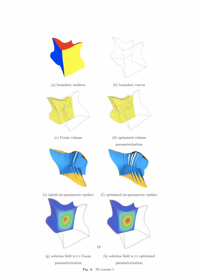
Fig. 6 shows a 3D example, which is drawn partly to illustrate the interior information of

the volume. The given boundary B-spline surfaces and curves are shown in Fig. 6 (a) and Fig.6

(b). Fig. 6 (c) presents the initial volume parametrization of computational domain constructed

by discrete Coons method. There are some self-intersections on the initial parameterization. Fig.

15

(a) boundary curves; (b) initial parameterization (c) initial iso-parametric net

(d) optimized

parameterization with

λ1 = 0 and λ2 = 1 ;

(e) optimized

parameterization with

λ1 = 1 and λ2 = 0

(f) optimized

parameterization with

λ1 = 0.5 and λ2 = 0.5

(g) optimized

parameterization with

λ1 = 0 and λ2 = 1

(h) optimized

parameterization with

λ1 = 1 and λ2 = 0

(i) optimized

parameterization with

λ1 = 0.5 and λ2 = 0.5

Fig. 3. 2D example I.

16

(a) (b)

Fig. 4. Simulation comparison for 2D example in Fig.3. (a) simulation error w.r.t Coons parameterization in

Fig.3(b); (b) simulation error w.r.t optimized parameterization in Fig.3(f) with same scale.

6 (d) shows the final volume parameterization of computational domain without self-intersections

constructed by variational harmonic method. To illustrate the quality of the parameterization,

the iso-parametric surfaces of the resulting B-spline volume are presented in Fig. 6 (e) and Fig.6

(f). Fig. 6 (g) and Fig.6 (h) presents the corresponding solution field obtained from the volume

parameterization in Fig. 6 (c) and Fig. 6 (d) . Obviously, the solution field in Fig. 6 (h) is more

smooth than the solution field in Fig. 6 (g), which indicates that the final volume parameterization

is better than the initial one. Another 3D example with complex geometry is shown in Fig.7.

Quantitative data of the examples presented in Fig. 3, Fig.5, Fig. 6 and Fig. 7 are summarized

in Table.1. Overall, the optimized parameterization obtained by our method has better quality,

and can achieve better simulation results than the initial Coons parameterization.

Remark 5.1. The optimization problem in this paper is multi-criterion and solved by aggregating

the criteria multiplied by weights λ1 and λ2. This straightforward approach has a well-known

drawback: the criteria may have different orders of magnitude and a naive choice of the weights

may yield a stronger decrease of a criterion, while others are not modified. To overcome this

difficulty, one may use adaptive weights: starting from equal weights, one adapts progressively

their values after some iterations, to achieve the same decrease for all criteria.

17

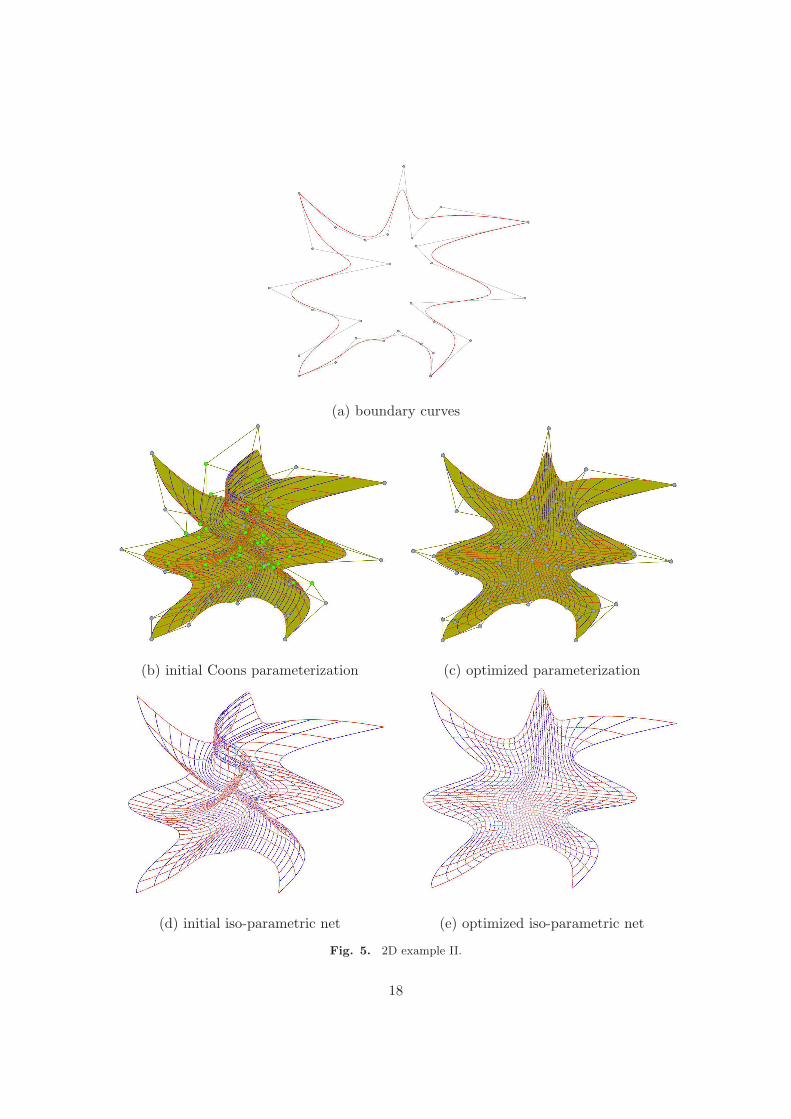
(a) boundary curves

(b) initial Coons parameterization (c) optimized parameterization

(d) initial iso-parametric net (e) optimized iso-parametric net

Fig. 5. 2D example II.

18

(a) boundary surfaces (b) boundary curves

(c) Coons volume (d) optimized volume

parameterization

(e) initial iso-parametric surface (f) optimized iso-parametric surface

(g) solution field w.r.t Coons

parameterization

(h) solution field w.r.t optimized

parameterization

Fig. 6. 3D example I.

19

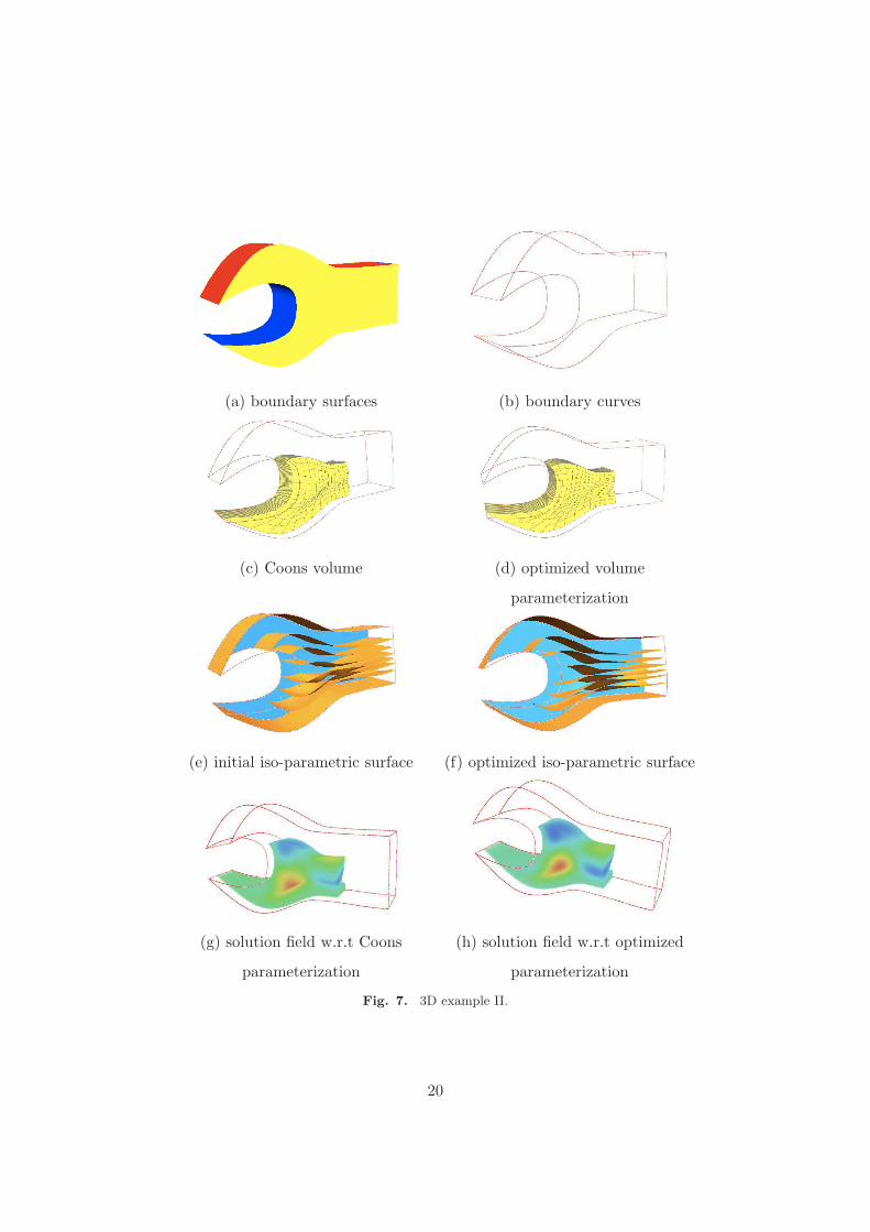
(a) boundary surfaces (b) boundary curves

(c) Coons volume (d) optimized volume

parameterization

(e) initial iso-parametric surface (f) optimized iso-parametric surface

(g) solution field w.r.t Coons

parameterization

(h) solution field w.r.t optimized

parameterization

Fig. 7. 3D example II.

20

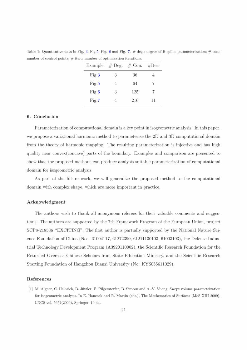
Table 1: Quantitative data in Fig. 3, Fig.5, Fig. 6 and Fig. 7. # deg.: degree of B-spline parameterization; # con.:

number of control points; # iter.: number of optimization iterations.

Example # Deg. # Con. #Iter.

Fig.3 3 36 4

Fig.5 4 64 7

Fig.6 3 125 7

Fig.7 4 216 11

6. Conclusion

Parameterization of computational domain is a key point in isogeometric analysis. In this paper,

we propose a variational harmonic method to parameterize the 2D and 3D computational domain

from the theory of harmonic mapping. The resulting parameterization is injective and has high

quality near convex(concave) parts of the boundary. Examples and comparison are presented to

show that the proposed methods can produce analysis-suitable parameterization of computational

domain for isogeometric analysis.

As part of the future work, we will generalize the proposed method to the computational

domain with complex shape, which are more important in practice.

Acknowledgment

The authors wish to thank all anonymous referees for their valuable comments and sugges-

tions. The authors are supported by the 7th Framework Program of the European Union, project

SCP8-218536 “EXCITING”. The first author is partially supported by the National Nature Sci-

ence Foundation of China (Nos. 61004117, 61272390, 61211130103, 61003193), the Defense Indus-

trial Technology Development Program (A3920110002), the Scientific Research Foundation for the

Returned Overseas Chinese Scholars from State Education Ministry, and the Scientific Research

Starting Foundation of Hangzhou Dianzi University (No. KYS055611029).

References

[1] M. Aigner, C. Heinrich, B. Juttler, E. Pilgerstorfer, B. Simeon and A.-V. Vuong. Swept volume parametrization

for isogeometric analysis. In E. Hancock and R. Martin (eds.), The Mathematics of Surfaces (MoS XIII 2009),

LNCS vol. 5654(2009), Springer, 19-44.

21

[2] I. Akkermana, Y. Bazilevsa, C.E. Keesb, M.W. Farthing. Isogeometric analysis of free-surface flow. Journal of

Computational Physics, 230(2011) 4137-4152.

[3] F. Auricchio, L.B. da Veiga, A. Buffa, C. Lovadina, A. Reali, and G. Sangalli. A fully locking-free isogeometric

approach for plane linear elasticity problems: A stream function formulation. Computer Methods in Applied

Mechanics and Engineering, 197(2007) 160-172.

[4] Y. Bazilevs, L. Beirao de Veiga, J.A. Cottrell, T.J.R. Hughes, and G. Sangalli. Isogeometric analysis: approxi-

mation, stability and error estimates for refined meshes. Mathematical Models and Methods in Applied Sciences,

6(2006) 1031-1090.

[5] Y. Bazilevs, V.M. Calo, T.J.R. Hughes, and Y. Zhang. Isogeometric fluid structure interaction: Theory, algo-

rithms, and computations. Computational Mechanics, 43(2008) 3-37.

[6] Y. Bazilevs, V.M. Calo, J.A. Cottrell, J. Evans, T.J.R. Hughes, S. Lipton, M.A. Scott, and T.W. Sederberg.

Isogeometric analysis using T-Splines. Computer Methods in Applied Mechanics and Engineering, 199(2010)

229-263.

[7] D. Burkhart, B. Hamann and G. Umlauf. Iso-geometric analysis based on Catmull-Clark subdivision solids.

Computer Graphics Forum, 29(2010) 1575-1584.

[8] E. Cohen, T. Martin, R.M. Kirby, T. Lyche and R.F. Riesenfeld, Analysis-aware Modeling: Understanding

Quality Considerations in Modeling for Isogeometric Analysis. Computer Methods in Applied Mechanics and

Engineering, 199(2010) 334-356.

[9] J.A. Cottrell, T.J.R. Hughes, Y. Bazilevs. Isogeometric Analysis: Toward Integration of CAD and FEA. Wiley,

2009

[10] J.A. Cottrell, T.J.R. Hughes, and A. Reali. Studies of refinement and continuity in isogeometric analysis.

Computer Methods in Applied Mechanics and Engineering, 196(2007) 4160-4183.

[11] J.A. Cottrell, A. Reali, Y. Bazilevs, and T.J.R. Hughes. Isogeometric analysis of structural vibrations. Computer

Methods in Applied Mechanics and Engineering, 195(2006) 5257-5296.

[12] N. Crouseilles, A. Ratnani, E. Sonnendrcker. An isogeometric analysis approach for the study of the gyrokinetic

quasi-neutrality equation. Journal of Computational Physics, 231(2012) 373-393.

[13] M. Dorfel, B. Juttler, and B. Simeon. Adaptive isogeometric analysis by local h-refinement with T-splines.

Computer Methods in Applied Mechanics and Engineering, 199(2010) 264-275.

[14] R. Duvigneau. An introduction to isogeometric analysis with application to thermal conduction. INRIA Research

Report RR-6957, June 2009

[15] J.M. Escobara, J.M. Casconb, E. Rodrıgueza, R. Montenegro. A new approach to solid modeling with trivariate

T-spline based on mesh optimization. Computer Methods in Applied Mechanics and Engineering, 200(2011)

3210-3222.

[16] G. Farin and D. Hansford. Discrete coons patches. Computer Aided Geometric Design, 16(1999) 691-700.

[17] P. Gill, W. Murray, M Wright. Practical Optimization. Springer, 1981.

[18] H. Gomez, V.M. Calo, Y. Bazilevs, and T.J.R. Hughes. Isogeometric analysis of the Cahn-Hilliard phase-field

model. Computer Methods in Applied Mechanics and Engineering, 197(2008) 4333-4352.

[19] T.J.R. Hughes, J.A. Cottrell, Y. Bazilevs. Isogeometric analysis: CAD, finite elements, NURBS, exact geometry,

22

and mesh refinement. Computer Methods in Applied Mechanics and Engineering, 194(2005) 4135-4195.

[20] X. Li, X. Guo, H. Wang, Y. He, X. Gu, H. Qin. Harmonic Volumetric Map- ping for Solid Modeling Applications.

Proc. of ACM Solid and Physical Modeling Symposium 2007, 109-120.

[21] T. Martin, E. Cohen, and R.M. Kirby. Volumetric parameterization and trivariate B-spline fitting using harmonic

functions. Computer Aided Geometric Design, 26(2009):648-664.

[22] T. Nguyen, B. Juttler. Using approximate implicitization for domain parameterization in isogeometric analysis.

International Conference on Curves and Surfaces, Avignon, France, 2010.

[23] N. Nguyen-Thanh, H. Nguyen-Xuan, S.P.A. Bordasd and T. Rabczuk. Isogeometric analysis using polynomial

splines over hierarchical T-meshes for two-dimensional elastic solids. Computer Methods in Applied Mechanics

and Engineering, 200(2011) 1892-1908.

[24] N. Nguyen-Thanh, J. Kiendl, H. Nguyen-Xuan, R. Wchner, K.U. Bletzinger, Y. Bazilevs, T. Rabczuk. Ro-

tation free isogeometric thin shell analysis using PHT-splines. Computer Methods in Applied Mechanics and

Engineering, 200(2011) 3410-3424.

[25] K.F. Pettersen, V. Skytt. Spline volume fairing. 7th International Conference on Curves and Surfaces. Avignon,

France, June 24-30, 2010, Lecture Notes in Computer Science, 6920(2012) 553-561.

[26] A. Ratnani, E. Sonnendrcker. An arbitrary high-order spline finite element solver for the time domain maxwell

equations. Journal of Scientific Computing, 51(2012) 87-106.

[27] S.P. Spekreijse. Elliptic grid generation based on Laplace equations and algebraic transformations. Journal of

Computational Physics, 118(1995) 38-61.

[28] C.L. Wang, K. Tang. Non-self-overlapping Hermite interpolation mapping: a practical solution for structured

quadrilateral meshing. Computer-Aided Design, 37(2005) 271-283.

[29] C.L. Wang, K. Tang. Non-self-overlapping structured grid generation on an n-sided surface. International Journal

for Numerical Methods in Fluids, 46(2004) 961-982.

[30] C.L. Wang, K. Tang. Algebraic grid generation on trimmed surface using non-self-overlapping Coons patch

mapping. International Journal for Numerical Methods in Engineering, 60(2004) 1259-1286.

[31] W. Wang, Y. Zhang, L. Liu, T. J.R. Hughes. Trivariate solid T-spline construction from boundary triangulations

with arbitrary genus topology. Computer-Aided Design, 45(2013) 351-360.

[32] N.J. Wu, T.K. Tsay, T.C. Yang, H.Y. Chang. Orthogonal grid generation of an irregular region using a local

polynomial collocation method. Journal of Computational Physics, 243(2013) 58-73.

[33] J. Xia, Y. He, X. Yin, S. Han, and X. Gu. Direct product volume parameterization using harmonic fields.

Proceedings of IEEE International Conference on Shape Modeling and Applications 2010, 3-12.

[34] J. Xia, Y. He, S. Han, C.W. Fu, F. Luo, and X. Gu. Parameterization of star shaped volumes using Green’s

functions. Proceedings of Geometric Modeling and Processing 2010, 6130(2010) 219-235.

[35] G. Xu, B. Mourrain, R. Duvigneau, A. Galligo. Optimal analysis-aware parameterization of computational

domain in 3D isogeometric analysis. Computer-Aided Design, 45(2013) 812-821.

[36] G. Xu, B. Mourrain, R. Duvigneau, A. Galligo. Parameterization of computational domain in isogeometric

analysis: methods and comparison. Computer Methods in Applied Mechanics and Engineering, 200(2011) 2021-

2031.

23

[37] G. Xu, B. Mourrain, R. Duvigneau, A. Galligo. Analysis-suitable volume parameterization of multi-block com-

putational domain in isogeometric applications. Computer-Aided Design, 45(2013) 395-404.

[38] Y. Zhang, W. Wang, T. J.R. Hughes. Solid T-spline construction from boundary representations for genus-zero

geometry. Computer Methods in Applied Mechanics and Engineering, 201(2012) 185-197.

[39] Y. Zhang, W. Wang, T. J.R. Hughes. Conformal solid T-spline construction from boundary T-spline represen-

tations. Computational Mechanics, 51(2013) 1051-1059.

[40] Y. Zhang, Y. Jia, S.Y. Wang. An improved nearly-orthogonal structured mesh generation system with smooth-

ness control functions. Journal of Computational Physics, 231(2012) 5289-5305.

[41] Y. Zhang, Y. Jia, S.Y. Wang. 2D nearly orthogonal mesh generation with controls on distortion function. Journal

of Computational Physics, 218(2006) 549-571.

24