Constraint Satisfaction pr oblems
60
Constraint Satisfaction problems
-
Upload
heather-carson -
Category
Documents
-
view
30 -
download
1
description
Constraint Satisfaction pr oblems. Outline. CSP? Backtracking for CSP Local search for CSPs Problem structure and decomposition. Constraint satisfaction problems. What is a CSP? Finite set of variables V 1 , V 2 , …, V n Finite set of constraints C 1 , C 2 , …, C m - PowerPoint PPT Presentation
Transcript of Constraint Satisfaction pr oblems

Constraint Satisfaction problems

2
Outline
• CSP?
• Backtracking for CSP
• Local search for CSPs
• Problem structure and decomposition

3
Constraint satisfaction problems• What is a CSP?
– Finite set of variables V1, V2, …, Vn
– Finite set of constraints C1, C2, …, Cm
– Nonempty domain of possible values for each variable DV1, DV2, … DVn
– Each constraint Ci limits the values that variables can take, e.g., V1 ≠ V2
• A state is defined as an assignment of values to some or all variables.
• Consistent assignment: assignment does not not violate the constraints.

4
Constraint satisfaction problems• An assignment is complete when every value is
mentioned. • A solution to a CSP is a complete assignment that
satisfies all constraints.• Some CSPs require a solution that maximizes an
objective function. • Applications: Scheduling the time of observations on
the Hubble Space Telescope, Floor planning, Map coloring, Cryptography

5
CSP example: map coloring
• Variables: WA, NT, Q, NSW, V, SA, T• Domains: Di={red,green,blue}• Constraints:adjacent regions must have different colors.
• E.g. WA NT • E.g. (WA,NT) {(red,green),(red,blue),(green,red),…}

6
CSP example: map coloring
• Solutions are assignments satisfying all constraints, e.g. {WA=red,NT=green,Q=red,NSW=green,V=red,SA=blue,T=green}

7
Constraint graph
• CSP benefits– Standard representation pattern– Generic goal and successor functions– Generic heuristics (no domain specific
expertise).
• Constraint graph = nodes are variables, edges show constraints.– Graph can be used to simplify search.
• e.g. Tasmania is an independent subproblem.

8
Varieties of CSPs• Discrete variables
– Finite domains; size d O(dn) complete assignments.• E.g. map coloring• Eight Queens
– Variables Q1, …Q8 – position of each queen is columns 1,…,8 – Each variable has domain {1,2,3,4,5,6,7,8}
• boolean CSPs, include. Boolean satisfiability (NP-complete)
– Infinite domains (integers, strings, etc.)• E.g. job scheduling, variables are start/end days for each job• Need a constraint language e.g StartJob1 +5 ≤ StartJob3.• Linear constraints solvable, nonlinear undecidable.
• Continuous variables– e.g. start/end times for Hubble Telescope observations.– Linear constraints solvable in poly time by LP methods.

9
Varieties of constraints• Unary constraints involve a single variable.
– e.g. SA green
• Binary constraints involve pairs of variables.– e.g. SA WA
• Higher-order constraints involve 3 or more variables.– e.g. cryptharithmetic column constraints.
• Preference (soft constraints) e.g. Prof X prefers teaching in the morning whereas Prof why Y prefers teaching in the afternoon. Assigning an afternoon slot for Prof X costs 2 points against the overall objective function whereas a morning slot costs 1. – often representable by a cost for each variable assignment
constrained optimization problems.

10
Example; cryptharithmetic
11
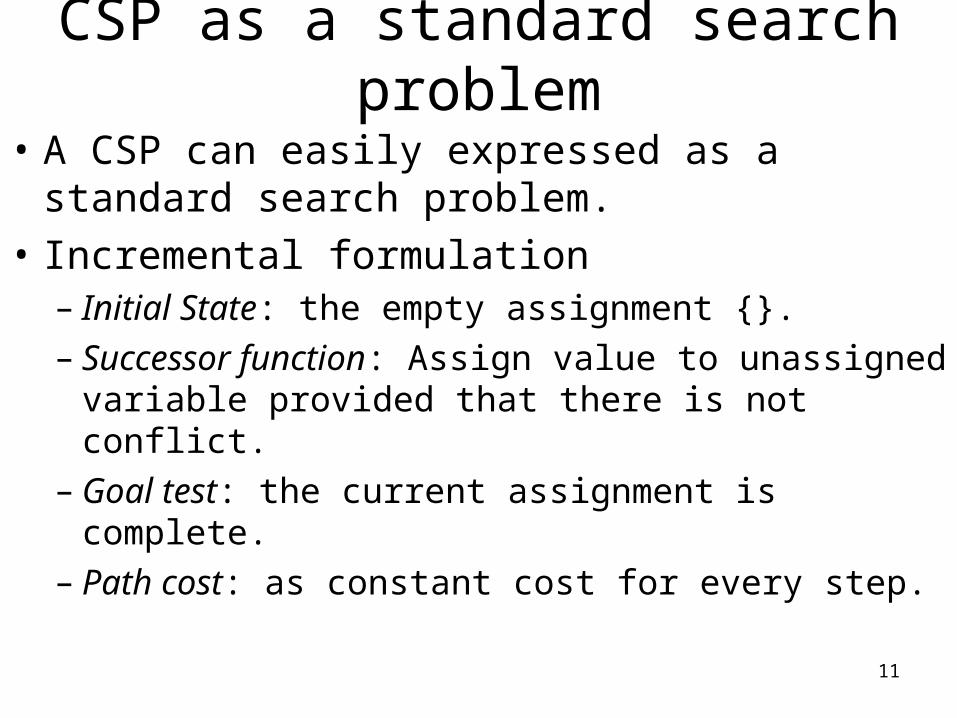
CSP as a standard search problem
• A CSP can easily expressed as a standard search problem.
• Incremental formulation– Initial State: the empty assignment {}.– Successor function: Assign value to unassigned
variable provided that there is not conflict.– Goal test: the current assignment is complete.– Path cost: as constant cost for every step.
12
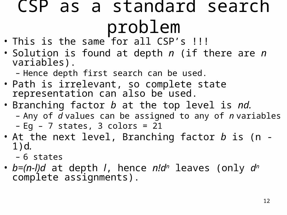
CSP as a standard search problem• This is the same for all CSP’s !!!• Solution is found at depth n (if there are n variables).
– Hence depth first search can be used.• Path is irrelevant, so complete state representation
can also be used.• Branching factor b at the top level is nd.
– Any of d values can be assigned to any of n variables– Eg – 7 states, 3 colors = 21
• At the next level, Branching factor b is (n -1)d. – 6 states
• b=(n-l)d at depth l, hence n!dn leaves (only dn complete assignments).

13
Commutativity
• CSPs are commutative.– The order of any given set of actions has no effect
on the outcome.– Example: choose colors for Australian territories
one at a time• [WA=red then NT=green] same as [NT=green then
WA=red]• All CSP search algorithms consider a single variable
assignment at a time there are dn leaves.

14
Backtracking search
• Cfr. Depth-first search
• Chooses values for one variable at a time and backtracks when a variable has no legal values left to assign.
• Uninformed algorithm– No good general performance (see table p. 143)

15
Backtracking searchfunction BACKTRACKING-SEARCH(csp) return a solution or failure
return RECURSIVE-BACKTRACKING({} , csp)
function RECURSIVE-BACKTRACKING(assignment, csp) return a solution or failureif assignment is complete then return assignmentvar SELECT-UNASSIGNED-VARIABLE(VARIABLES[csp],assignment,csp)for each value in ORDER-DOMAIN-VALUES(var, assignment, csp) do
if value is consistent with assignment according to CONSTRAINTS[csp] then
add {var=value} to assignment result RRECURSIVE-BACTRACKING(assignment, csp)if result failure then return resultremove {var=value} from assignment
return failure

16
Backtracking example

17
Backtracking example

18
Backtracking example

19
Backtracking example

20
Improving backtracking efficiency
• Previous improvements introduce heuristics
• General-purpose methods can give huge gains in speed:– Which variable should be assigned next?– In what order should its values be tried?– Can we detect inevitable failure early?– Can we take advantage of problem structure?

21
Minimum remaining values
var SELECT-UNASSIGNED-VARIABLE(VARIABLES[csp],assignment,csp)
• A.k.a. most constrained variable heuristic• Rule: choose variable with the fewest legal moves
– picks a variable that is most likely to cause a failure – prunes search tree
– Variable X with zero legal values remaining will be selected. avoids pointless searches through other variables which will always fail when X is finally selected
• Which variable shall we try first?

22
Degree heuristic
• Use degree heuristic• Rule: select variable that is involved in the largest number of
constraints on other unassigned variables.• Degree heuristic is very useful as a tie breaker.• In what order should its values be tried?

23
Least constraining value
• Least constraining value heuristic• Rule: given a variable choose the least constraining value i.e.
the one that leaves the maximum flexibility for subsequent variable assignments.

24
Forward checking
• Can we detect inevitable failure early?– And avoid it later?
• Forward checking idea: keep track of remaining legal values for unassigned variables.
• Terminate search when any variable has no legal values.

25
Forward checking
• Assign {WA=red}• Effects on other variables connected by constraints with WA
– NT can no longer be red– SA can no longer be red

26
Forward checking
• Assign {Q=green}
• Effects on other variables connected by constraints with WA– NT can no longer be green
– NSW can no longer be green
– SA can no longer be green
• MRV heuristic will automatically select NT and SA next, why?

27
Forward checking
• If V is assigned blue
• Effects on other variables connected by constraints with WA– SA is empty
– NSW can no longer be blue
• FC has detected that partial assignment is inconsistent with the constraints and backtracking can occur.

28
Example: 4-Queens Problem
1
3
2
4
32 41
X1{1,2,3,4}
X3{1,2,3,4}
X4{1,2,3,4}
X2{1,2,3,4}
[4-Queens slides copied from B.J. Dorr CMSC 421 course on AI]

29
Example: 4-Queens Problem
1
3
2
4
32 41
X1{1,2,3,4}
X3{1,2,3,4}
X4{1,2,3,4}
X2{1,2,3,4}

30
Example: 4-Queens Problem
1
3
2
4
32 41
X1{1,2,3,4}
X3{ ,2, ,4}
X4{ ,2,3, }
X2{ , ,3,4}

31
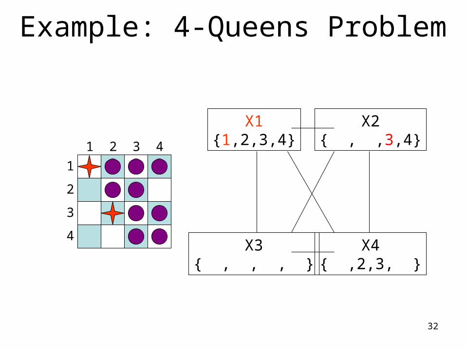
Example: 4-Queens Problem
1
3
2
4
32 41
X1{1,2,3,4}
X3{ ,2, ,4}
X4{ ,2,3, }
X2{ , ,3,4}
32
Example: 4-Queens Problem
1
3
2
4
32 41
X1{1,2,3,4}
X3{ , , , }
X4{ ,2,3, }
X2{ , ,3,4}

33
Example: 4-Queens Problem
1
3
2
4
32 41
X1{ ,2,3,4}
X3{1,2,3,4}
X4{1,2,3,4}
X2{1,2,3,4}

34
Example: 4-Queens Problem
1
3
2
4
32 41
X1{ ,2,3,4}
X3{1, ,3, }
X4{1, ,3,4}
X2{ , , ,4}

35
Example: 4-Queens Problem
1
3
2
4
32 41
X1{ ,2,3,4}
X3{1, ,3, }
X4{1, ,3,4}
X2{ , , ,4}

36
Example: 4-Queens Problem
1
3
2
4
32 41
X1{ ,2,3,4}
X3{1, , , }
X4{1, ,3, }
X2{ , , ,4}

37
Example: 4-Queens Problem
1
3
2
4
32 41
X1{ ,2,3,4}
X3{1, , , }
X4{1, ,3, }
X2{ , , ,4}

38
Example: 4-Queens Problem
1
3
2
4
32 41
X1{ ,2,3,4}
X3{1, , , }
X4{ , ,3, }
X2{ , , ,4}

39
Example: 4-Queens Problem
1
3
2
4
32 41
X1{ ,2,3,4}
X3{1, , , }
X4{ , ,3, }
X2{ , , ,4}
40
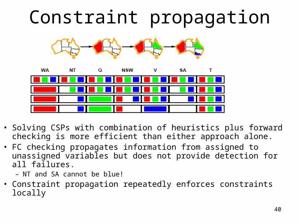
Constraint propagation
• Solving CSPs with combination of heuristics plus forward checking is more efficient than either approach alone.
• FC checking propagates information from assigned to unassigned variables but does not provide detection for all failures.– NT and SA cannot be blue!
• Constraint propagation repeatedly enforces constraints locally

41
Arc consistency
• X Y is consistent ifffor every value x of X there is some allowed y
• SA NSW is consistent iffSA=blue and NSW=red

42
Arc consistency
• X Y is consistent ifffor every value x of X there is some allowed y
• NSW SA is consistent iffNSW=red and SA=blueNSW=blue and SA=???
Arc can be made consistent by removing blue from NSW

43
Arc consistency
• Arc can be made consistent by removing blue from NSW• RECHECK neighbours !!
– Remove red from V

44
Arc consistency
• Arc can be made consistent by removing blue from NSW• RECHECK neighbours !!
– Remove red from V
• Arc consistency detects failure earlier than FC• Can be run as a preprocessor or after each assignment.
– Repeated until no inconsistency remains

45
Arc consistency algorithm
function AC-3(csp) return the CSP, possibly with reduced domains
inputs: csp, a binary csp with variables {X1, X2, …, Xn}local variables: queue, a queue of arcs initially the arcs in csp
while queue is not empty do
(Xi, Xj) REMOVE-FIRST(queue)
if REMOVE-INCONSISTENT-VALUES(Xi, Xj) then
for each Xk in NEIGHBORS[Xi ] do
add (Xi, Xj) to queue
function REMOVE-INCONSISTENT-VALUES(Xi, Xj) return true iff we remove a valueremoved false
for each x in DOMAIN[Xi] do
if no value y in DOMAIN[Xi] allows (x,y) to satisfy the constraints between Xi and Xj
then delete x from DOMAIN[Xi]; removed truereturn removed

46
K-consistency• Arc consistency does not detect all inconsistencies:
– Partial assignment {WA=red, NSW=red} is inconsistent.
• Stronger forms of propagation can be defined using the notion of k-consistency.
• A CSP is k-consistent if for any set of k-1 variables and for any consistent assignment to those variables, a consistent value can always be assigned to any kth variable.– E.g. 1-consistency or node-consistency– E.g. 2-consistency or arc-consistency– E.g. 3-consistency or path-consistency
47
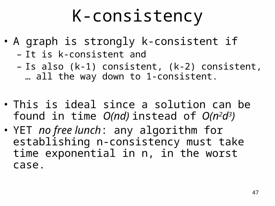
K-consistency• A graph is strongly k-consistent if
– It is k-consistent and– Is also (k-1) consistent, (k-2) consistent, … all the way down
to 1-consistent.
• This is ideal since a solution can be found in time O(nd) instead of O(n2d3)
• YET no free lunch: any algorithm for establishing n-consistency must take time exponential in n, in the worst case.

48
Further improvements
• Checking special constraints – use special purpose algorithms rather than general purpose methods– Checking Alldif(…) constraint
• E.g. {WA=red, NSW=red}
– Checking Atmost(…) constraint

49
Further improvements• Algorithm
– Remove any variable in the constraint that has a singleton domain
– delete that variable’s value from the domains of the remaining variables
– Repeat – if empty domain is produced or that there are more variables
than domain values left – inconsistency detected
• Partial assignment {WA = red, NSW = red}– Applying arc inconsistency of the domain of each variable is
reduced to {green, blue}– three variables and only two colors – constraint is violated
50
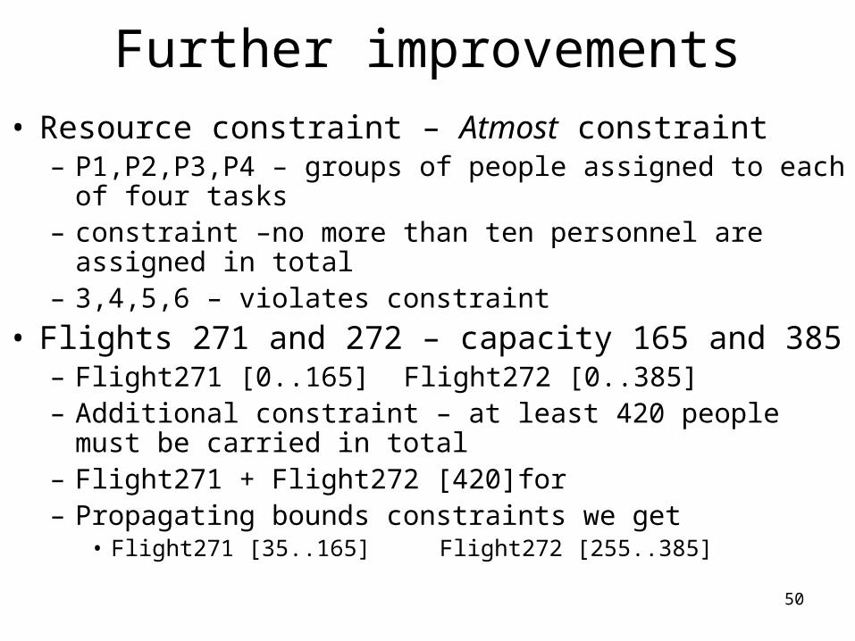
Further improvements• Resource constraint – Atmost constraint
– P1,P2,P3,P4 – groups of people assigned to each of four tasks
– constraint –no more than ten personnel are assigned in total – 3,4,5,6 – violates constraint
• Flights 271 and 272 – capacity 165 and 385– Flight271 [0..165] Flight272 [0..385]– Additional constraint – at least 420 people must be carried in
total – Flight271 + Flight272 [420]for – Propagating bounds constraints we get
• Flight271 [35..165] Flight272 [255..385]
51
Further improvements
• CSP is bounds consistent – If for every variable X, and for both the lower bound
and upper bound values of X, the exists some value of Y that satisfies the constraint between X and Y, for every variable Y
52
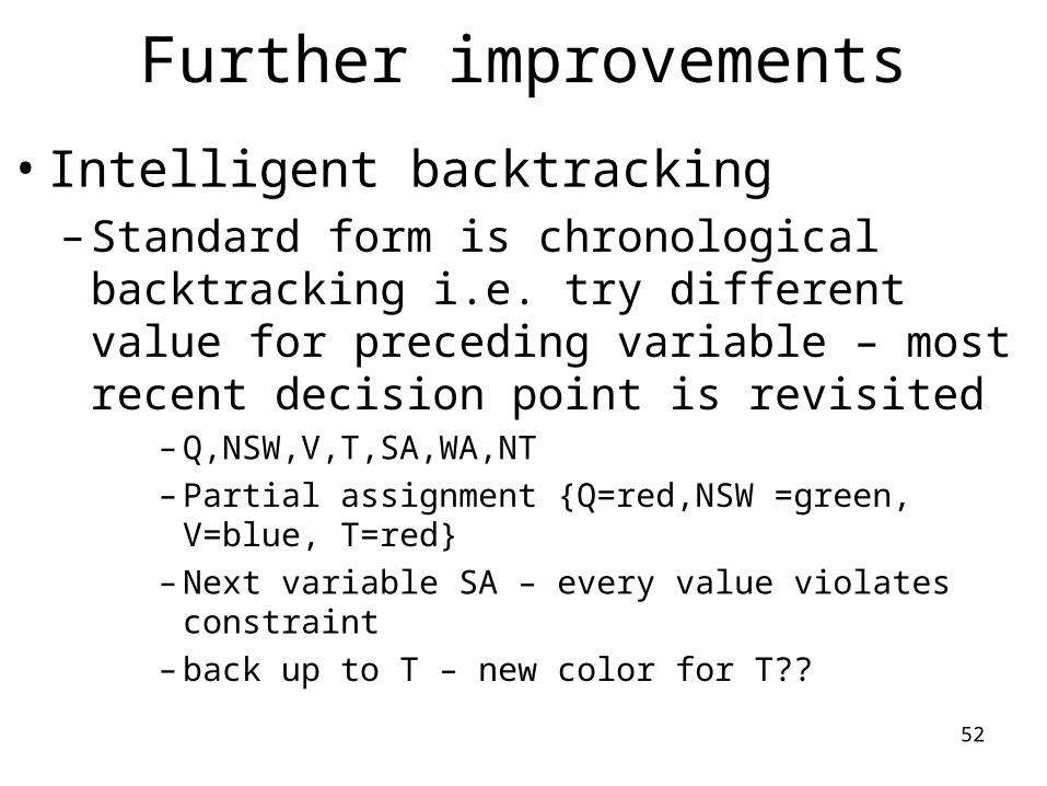
Further improvements
• Intelligent backtracking– Standard form is chronological backtracking
i.e. try different value for preceding variable – most recent decision point is revisited
– Q,NSW,V,T,SA,WA,NT– Partial assignment {Q=red,NSW =green, V=blue,
T=red}– Next variable SA – every value violates constraint – back up to T – new color for T??

53
Further improvements
– More intelligent, backtrack to conflict set.• Set of variables that caused the failure or set of
previously assigned variables that are connected to X by constraints.
– Conflict set – {Q,NSW,V }
• Backjumping moves back to most recent element of the conflict set.
– Jump over T and try a new value for V
• Forward checking can be used to determine conflict set

54
Local search for CSP• Use complete-state representation
– Initial state assigns a value to every variable • 8-Queens – initial state – random configuration of 8 Queens in 8 columns
– Successor function changes value of one variable at a time • Successor function – picks one queen and considers moving it elsewhere in
its columna
• For CSPs– allow states with unsatisfied constraints– operators reassign variable values
• Variable selection: randomly select any conflicted variable• Value selection: min-conflicts heuristic
– Select new value that results in a minimum number of conflicts with the other variables

55
Local search for CSPfunction MIN-CONFLICTS(csp, max_steps) return solution or failure
inputs: csp, a constraint satisfaction problemmax_steps, the number of steps allowed before giving up
current an initial complete assignment for cspfor i = 1 to max_steps do
if current is a solution for csp then return currentvar a randomly chosen, conflicted variable from VARIABLES[csp]value the value v for var that minimizes CONFLICTS(var,v,current,csp)set var = value in current
return faiilure

56
Min-conflicts example 1
• Use of min-conflicts heuristic in hill-climbing.
h=5 h=3 h=1

57
Min-conflicts example 2
• A two-step solution for an 8-queens problem using min-conflicts heuristic.
• At each stage a queen is chosen for reassignment in its column.• The algorithm moves the queen to the min-conflict square
breaking ties randomly.

58
Problem structure
• How can the problem structure help to find a solution quickly?• Subproblem identification is important:
– Coloring Tasmania and mainland are independent subproblems– Identifiable as connected components of constrained graph.
– If assignment Si is a solution of CSPi then is a solution of
• Improves performance
i iS
i iCSP

59
Problem structure
• Suppose each problem has c variables out of a total of n.• Worst case solution cost is O(n/c dc), i.e. linear in n
– Instead of O(d n), exponential in n
• E.g. n= 80, c= 20, d=2– 280 = 4 billion years at 1 million nodes/sec.– 4 * 220= .4 second at 1 million nodes/sec
60
Summary• CSPs are a special kind of problem: states defined by values
of a fixed set of variables, goal test defined by constraints on variable values
• Backtracking=depth-first search with one variable assigned per node
• Variable ordering and value selection heuristics help significantly
• Forward checking prevents assignments that lead to failure.• Constraint propagation does additional work to constrain
values and detect inconsistencies.• The CSP representation allows analysis of problem structure.• Iterative min-conflicts is usually effective in practice.