Constraint satisfaction inference for discrete sequence processing in NLP Antal van den Bosch ILK /...

Constraint satisfaction inference for discrete sequence processing in

NLP

Antal van den BoschILK / CL and AI, Tilburg University

DCUDublin April 19, 2006

(work with Sander Canisius and Walter Daelemans)

Constraint satisfaction inference for discrete sequence processing in

NLPTalk overview

• How to map sequences to sequences, not output tokens?

• Case studies: syntactic and semantic chunking

• Discrete versus probabilistic classifiers

• Constraint satisfaction inference• Discussion

How to map sequences to sequences?

• Machine learning’s pet solution:– Local-context windowing (NETtalk)– One-shot prediction of single output tokens.

– Concatenation of predicted tokens.

The near-sightedness problem

• A local window never captures long-distance information.

• No coordination of individual output tokens.

• Long-distance information does exist; holistic coordination is needed.

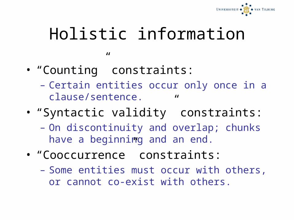
Holistic information

• “Counting” constraints:– Certain entities occur only once in a clause/sentence.

• “Syntactic validity” constraints:– On discontinuity and overlap; chunks have a beginning and an end.

• “Cooccurrence” constraints:– Some entities must occur with others, or cannot co-exist with others.

Solution 1: Feedback

• Recurrent networks in ANN (Elman, 1991; Sun & Giles, 2001), e.g. word prediction.

• Memory-based tagger (Daelemans, Zavrel, Berck, and Gillis, 1996).

• Maximum-entropy tagger (Ratnaparkhi, 1996).

Feedback disadvantage

• Label bias problem (Lafferty, McCallum, and Pereira, 2001).

– Previous prediction is an important source of information.

– Classifier is compelled to take its own prediction as correct.

– Cascading errors result.

Label bias problem

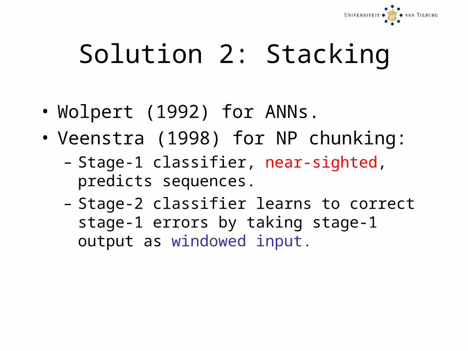
Solution 2: Stacking

• Wolpert (1992) for ANNs.• Veenstra (1998) for NP chunking:

– Stage-1 classifier, near-sighted, predicts sequences.

– Stage-2 classifier learns to correct stage-1 errors by taking stage-1 output as windowed input.

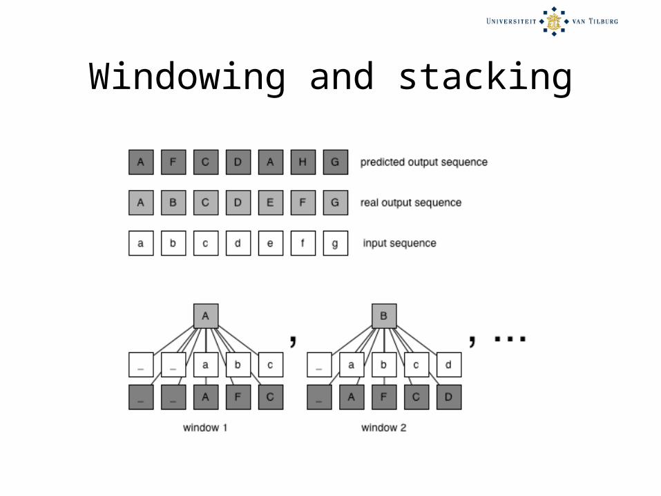
Windowing and stacking

Stacking disadvantages

• Practical issues:– Ideally, train stage-2 on cross-validated output of stage-1, not “perfect” output.

– Costly procedure.– Total architecture: two full classifiers.

• Local, not global error correction.

What exactly is the problem with mapping to

sequences?• Born in Made, The Netherlands

O_O_B-LOC_O_B-LOC_I-LOC

• Multi-class classification with 100s or 1000s of classes?– Lack of generalization

• Some ML algorithms cannot cope very well.– SVMs– Rule learners, decision trees

• However, others can.– Naïve Bayes, Maximum-entropy– Memory-based learning

Solution 3: n-gram subsequences

• Retain windowing approach, but• Predict overlapping n-grams of output tokens.

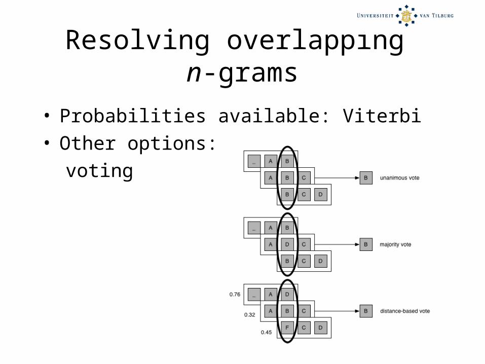
Resolving overlapping n-grams

• Probabilities available: Viterbi• Other options:

voting

N-gram+voting disadvantages

• Classifier predicts syntactically valid trigrams, but

• After resolving overlap, only local error correction.

• End result is still a concatenation of local uncoordinated decisions.

• Number of classes increases (problematic for some ML).

Learning linguistic sequences

Talk overview





Four “chunking” tasks

• English base-phrase chunking– CoNLL-2000, WSJ

• English named-entity recognition– CoNLL-2003, Reuters

• Dutch medical concept chunking– IMIX/Rolaquad, medical encyclopedia

• English protein-related entity chunking– Genia, Medline abstracts

Treated the same way

• IOB-tagging.• Windowing:

– 3-1-3 words– 3-1-3 predicted PoS tags (WSJ / Wotan)

• No seedlists, suffix/prefix, capitalization, …

• Memory-based learning and maximum-entropy modeling

• MBL: automatic parameter optimization (paramsearch, Van den Bosch, 2004)

IOB-codes for chunks: step 1, PTB-II WSJ

((S (ADVP-TMP Once) (NP-SBJ-1 he) (VP was (VP held (NP *-1) (PP-TMP for (NP three months)) (PP without (S-NOM (NP-SBJ *-1) (VP being (VP charged)))))) .))

IOB codes for chunks:Flatten tree

[Once]ADVP

[he]NP

[was held]VP

[for]PP

[three months]NP

[without]PP

[being charged]VP

Example: Instancesfeature 1 feature 2 feature 3 class(word -1) (word 0) (word +1)

1. _ Once he I-ADVP 2. Once he was I-NP3. he was held I-VP4. was held for I-VP5. held for three I-PP6. for three months I-NP7. three months without I-NP8. months without being I-PP9. without being charged I-VP10. being charged . I-VP11. charged . _ O

MBL

• Memory-based learning– k-NN classifier (Fix and Hodges, 1951; Cover and Hart, 1967; Aha et al., 1991), Daelemans et al.

– Discrete point-wise classifier– Implementation used: TiMBL (Tilburg Memory-Based Learner)

Memory-based learning and classification

• Learning:– Store instances in memory

• Classification:– Given new test instance X,– Compare it to all memory instances

• Compute a distance between X and memory instance Y

• Update the top k of closest instances (nearest neighbors)

– When done, take the majority class of the k nearest neighbors as the class of X

Similarity / distance

• A nearest neighbor has the smallest distance, or the largest similarity

• Computed with a distance function• TiMBL offers two basic distance functions:– Overlap– MVDM (Stanfill & Waltz, 1986; Cost & Salzberg, 1989)

• Feature weighting• Exemplar weighting• Distance-weighted class voting

The Overlap distance function

• “Count the number of mismatching features”

€

Δ(X,Y ) = δ(x i,y i)i=1

n

∑

€

δ(x i,y i) =

x i − y imaxi− mini

if numeric,else

0 if x i = y i1 if x i ≠ y i

⎧

⎨

⎪ ⎪

⎩

⎪ ⎪

The MVDM distance function

• Estimate a numeric “distance” between pairs of values– “e” is more like “i” than like “p” in a phonetic task

– “book” is more like “document” than like “the” in a parsing task

€

δ(x i,y i) = P(C j | x i) − P(C j | y i)j=1

n

∑

Feature weighting

• Some features are more important than others

• TiMBL metrics: Information Gain, Gain Ratio, Chi Square, Shared Variance

• Ex. IG:– Compute data base entropy– For each feature,

• partition the data base on all values of that feature– For all values, compute the sub-data base entropy

• Take the weighted average entropy over all partitioned subdatabases

• The difference between the “partitioned” entropy and the overall entropy is the feature’s Information Gain

Feature weighting in the distance function

• Mismatching on a more important feature gives a larger distance

• Factor in the distance function:

€

Δ(X,Y ) = IGiδ(x i,y i)i=1

n

∑

Distance weighting

• Relation between larger k and smoothing

• Subtle extension: making more distant neighbors count less in the class vote– Linear inverse of distance (w.r.t. max)

– Inverse of distance– Exponential decay

Current practice

• Default TiMBL settings: – k=1, Overlap, GR, no distance weighting– Work well for some morpho-phonological tasks

• Rules of thumb:– Combine MVDM with bigger k– Combine distance weighting with bigger k– Very good bet: higher k, MVDM, GR, distance weighting

– Especially for sentence and text level tasks

Base phrase chunking

• 211,727 training, 47,377 test examples

• 22 classes

• [He]NP [reckons]VP [the current account deficit]NP [will narrow]VP [to]PP [only $ 1.8 billion]NP [in]PP [September]NP .

Named entity recognition


• 8 classes

• [U.N.]organization official [Ekeus]person heads for [Baghdad]location

Medical concept chunking


• 24 classes

• Bij [infantiel botulisme]disease kunnen in extreme gevallen [ademhalingsproblemen]symptom en [algehele lusteloosheid]symptom optreden.

Protein-related concept chunking


• 51 classes• Most hybrids express both [KBF1]protein and [NF-kappa B]protein in their nuclei , but one hybrid expresses only [KBF1]protein .

Results: feedback in MBT

Task BaselineWith

feedbackError red.

Base-phrase chunking

91.9 93.0 14%

Named-entity recog.

77.2 78.1 4%

Medical chunking

64.7 67.0 7%

Protein chunking

55.8 62.3 15%

Results: stacking

Task BaselineWith

stackingError red.


91.9 92.6 9%

Named-entity recog.

77.2 78.9 7%

Medical chunking

64.7 67.0 7%

Protein chunking

55.8 57.2 3%

Results: trigram classes

Task BaselineWith

trigramError red.


91.9 92.7 10%

Named-entity recog.

77.2 80.2 13%

Medical chunking

64.7 67.5 8%

Protein chunking

55.8 60.1 10%

Numbers of trigram classes

Task unigrams trigrams


22 846

Named-entity recog.

8 138

Medical chunking

24 578

Protein chunking

51 1471

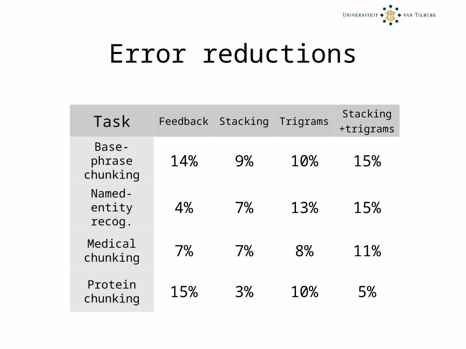
Error reductions

Task Feedback Stacking TrigramsStacking+trigrams


14% 9% 10% 15%

Named-entity recog.

4% 7% 13% 15%

Medical chunking 7% 7% 8% 11%

Protein chunking 15% 3% 10% 5%


Talk overview





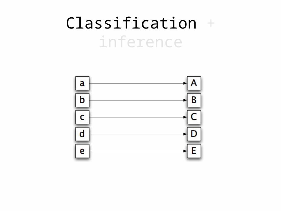
Classification + inference

Comparative study

• Base discrete classifier: Maximum-entropy model (Zhang Le, maxent)– Extended with feedback, stacking, trigrams, combinations

• Compared against– Conditional Markov Models (Ratnaparkhi, 1996)

– Maximum-entropy Markov Models (McCallum, Freitag, and Pereira, 2000)

– Conditional Random Fields (Lafferty, McCallum, and Pereira, 2001)

• On Medical & Protein chunking

Maximum entropy

• Probabilistic model: conditional distribution p(C|x) (= probability matrix between classes and values) with maximal entropy H(p)

• Given a collection of facts, choose a model which is consistent with all the facts, but otherwise as uniform as possible

• Maximize entropy in matrix through iterative process:– IIS, GIS (Improved/Generalized Iterative Scaling)– L-BFGS

• Discretized!

Results: discrete Maxent variants

TaskBaselin

eFeedbac

kStackin

gTrigram

Medical chunking 61.5 63.9 62.0 63.1

Protein chunking 54.5 62.1 56.5 58.8

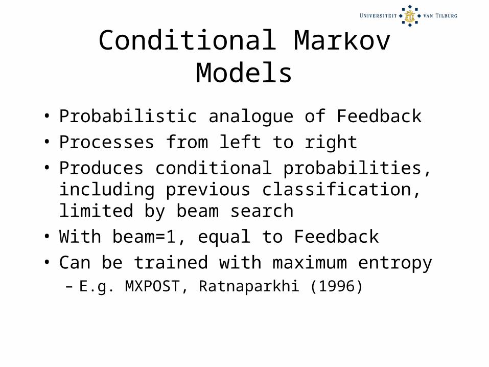
Conditional Markov Models

• Probabilistic analogue of Feedback• Processes from left to right• Produces conditional probabilities, including previous classification, limited by beam search

• With beam=1, equal to Feedback• Can be trained with maximum entropy

– E.g. MXPOST, Ratnaparkhi (1996)

Feedback vs. CMM

Task Baseline Feedback CMM

Medical chunking 61.5 63.9 63.9

Protein chunking 54.5 62.1 62.4

Maximum-entropy Markov Models

• Probabilistic state machines:– Given previous label and current input vector, produces conditional distributions for current output token.

– Separate conditional distributions for each output token (state).

• Again directional, so suffers from label bias problem.

• Specialized Viterbi search.

Conditional Random Fields

• Aimed to repair weakness of MEMMs.

• Instead of separate model for each state,

• A single model for likelihood of sequence (e.g. class bigrams).

• Viterbi search.

Discrete classifiers vs.

MEMM and CRF

TaskBest

discrete MBL

Best discret

e Maxent

CMM MEMM CRF

Medical chunking 67.51 63.93 63.9 63.7 63.4

Protein chunking 62.32 62.14 62.4 62.1 62.8

3 Maxent with feedback

4 Maxent with feedback

1 MBL with trigrams

2 MBL with feedback


Talk overview





(Many classes - no problem for MBL)

Constraint satisfaction inference

Results: Shallow parsing and IE

taskBase

classifier

Voting CSI Oracle

CoNLL Chunking 91.9 92.7 93.1 95.8

CoNLL NER 77.2 80.2 81.8 86.5

Genia (bio-NER) 55.8 60.1 61.8 69.8

ROLAQUAD (med-NER) 64.7 67.5 68.9 74.9

Results: Morpho-phonology

taskBase

classifierCSI

Letter-phoneme English

79.0 ± 0.82

84.5 ± 0.82

Letter-phoneme Dutch

92.8 ± 0.25

94.4 ± 0.25

Morphological segmentation English

80.0 ± 0.75

85.4 ± 0.71

Morphological segmentation Dutch

41.3 ± 0.48

51.9 ± 0.48

Discussion

• The classification+inference paradigm fits both probabilistic and discrete classifiers– Necessary component: search space to look for globally likely solutions• Viterbi search in class distributions• Constraint satisfaction inference in overlapping trigram space

• Discrete vs probabilistic?– CMM beam search hardly matters– Best discrete Maxent MEMM! (but CRF is better)– Discrete classifiers: lightning-fast training vs. convergence training of MEMM / CRF.

– Don’t write off discrete classifiers.

Software

• TiMBL, Tilburg Memory-Based Learner (5.1)• MBT, Memory-based Tagger (2.0)• Paramsearch (1.0)• CMM, MEMM

http://ilk.uvt.nl

• Maxent (Zhang Le, Edinburgh, 20041229)http://homepages.inf.ed.ac.uk/

s0450736/maxent_toolkit.html

• Mallet (McCallum et al., UMass)http://

mallet.cs.umass.edu

http://homepages.inf.ed.ac.uk/

Paramsearch

• (Van den Bosch, 2004, Proc. of BNAIC)

• Machine learning meta problem:– Algorithmic parameters change bias

• Description length and noise bias• Eagerness bias

– Can make huge difference (Daelemans & Hoste, ECML 2003)

– Different parameter settings = functionally different system

– But good settings not predictable

Known solution

• Classifier wrapping (Kohavi, 1997)– Training set train & validate sets– Test different setting combinations– Pick best-performing

• Danger of overfitting• Costly

Optimizing wrapping

• Worst case: exhaustive testing of “all” combinations of parameter settings (pseudo-exhaustive)

• Simple optimization:– Not test all settings

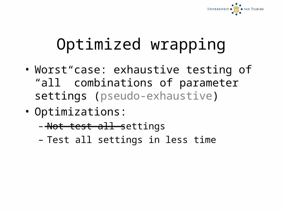
Optimized wrapping


• Optimizations:– Not test all settings– Test all settings in less time

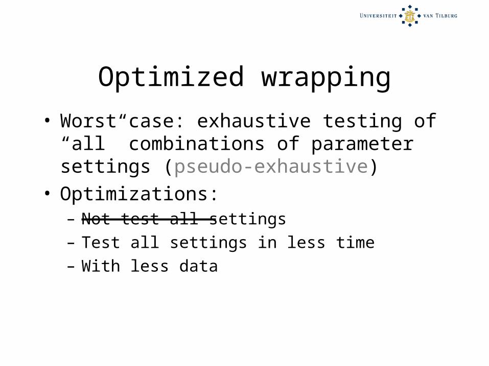
Optimized wrapping


• Optimizations:– Not test all settings– Test all settings in less time– With less data

Progressive sampling

• Provost, Jensen, & Oates (1999)• Setting:

– 1 algorithm (parameters already set)– Growing samples of data set

• Find point in learning curve at which no additional learning is needed

Wrapped progressive sampling

• Use increasing amounts of data• While validating decreasing numbers of setting combinations

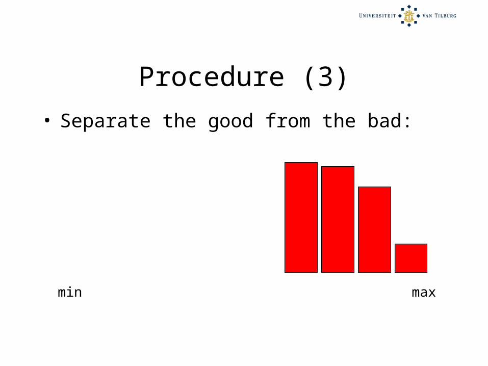
• E.g.,– Test “all” settings combinations on a small but sufficient subset

– Increase amount of data stepwise– At each step, discard lower-performing setting combinations

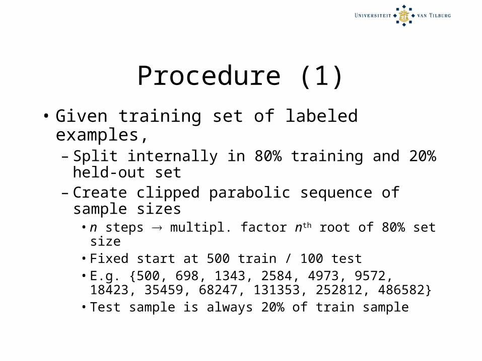
Procedure (1)• Given training set of labeled examples,– Split internally in 80% training and 20% held-out set

– Create clipped parabolic sequence of sample sizes•n steps multipl. factor nth root of 80% set size

•Fixed start at 500 train / 100 test•E.g. {500, 698, 1343, 2584, 4973, 9572, 18423, 35459, 68247, 131353, 252812, 486582}

•Test sample is always 20% of train sample

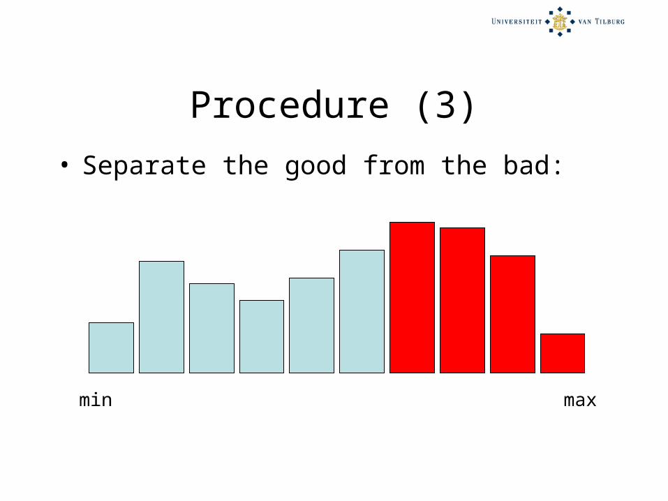
Procedure (2)• Create pseudo-exhaustive pool of all parameter setting combinations

• Loop:– Apply current pool to current train/test sample pair

– Separate good from bad part of pool– Current pool := good part of pool– Increase step

• Until one best setting combination left, or all steps performed (random pick)

Procedure (3)

• Separate the good from the bad:

min max

“Mountaineering competition”

Customizations

algorithm # parametersTotal # setting

combinations

Ripper (Cohen, 1995) 6 648

C4.5 (Quinlan, 1993) 3 360

Maxent (Giuasu et al, 1985) 2 11

Winnow (Littlestone, 1988) 5 1200

IB1 (Aha et al, 1991) 5 925

Experiments: datasetsTask # Examples # Features # Classes Class entropy

audiology 228 69 24 3.41

bridges 110 7 8 2.50

soybean 685 35 19 3.84

tic-tac-toe 960 9 2 0.93

votes 437 16 2 0.96

car 1730 6 4 1.21

connect-4 67559 42 3 1.22

kr-vs-kp 3197 36 2 1.00

splice 3192 60 3 1.48

nursery 12961 8 5 1.72

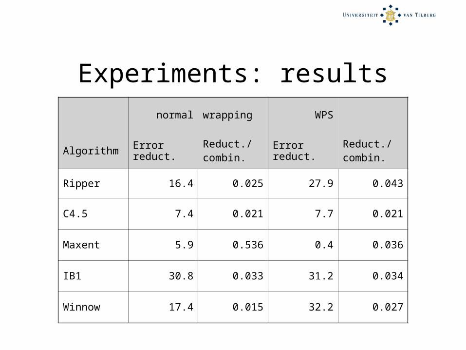
Experiments: resultsnormal wrapping WPS

Algorithm Error reduct.

Reduct./combin.

Error reduct.

Reduct./combin.

Ripper 16.4 0.025 27.9 0.043

C4.5 7.4 0.021 7.7 0.021

Maxent 5.9 0.536 0.4 0.036

IB1 30.8 0.033 31.2 0.034

Winnow 17.4 0.015 32.2 0.027

Paramsearch roundup

• Large improvements with algorithms with many parameters.

• “Guaranteed” gain of 0.02% per added combination.

• Still to do: interaction with feature selection.

Thank you

Constraint satisfaction inference for discrete sequence processing in NLP Antal van den Bosch ILK /...

Documents

Transcript of Constraint satisfaction inference for discrete sequence processing in NLP Antal van den Bosch ILK /...