Constraining Inflation Histories with the CMB & Large Scale Structure

Dynamical & Resolution Trajectories for Inflation then & now

Dick Bond

CMBology

ForegroundsCBI, Planck

ForegroundsCBI, Planck

SecondaryAnisotropies

(tSZ, kSZ, reion)

SecondaryAnisotropies

(tSZ, kSZ, reion)

Non-Gaussianity(Boom, CBI, WMAP)

Non-Gaussianity(Boom, CBI, WMAP)

Polarization ofthe CMB, Gravity Waves

(CBI, Boom, Planck, Spider)

Polarization ofthe CMB, Gravity Waves

(CBI, Boom, Planck, Spider)

Dark Energy Histories(& CFHTLS-SN+WL)

Dark Energy Histories(& CFHTLS-SN+WL)

subdominant phenomena

(isocurvature, BSI)

subdominant phenomena

(isocurvature, BSI)

Inflation Histories(CMBall+LSS)

Inflation Histories(CMBall+LSS)

Probing the linear & nonlinear cosmic web

Probing the linear & nonlinear cosmic web

R ? z = 0

Primary Anisotropies

•Tightly coupled Photon-Baryon fluid oscillations

• viscously damped

•Linear regime of perturbations

•Gravitational redshifting

Dec

oupl

ing

LSS

Secondary Anisotropies

•Non-Linear Evolution

•Weak Lensing

•Thermal and Kinetic SZ effect

•Etc.

z? ø 1100

19 Mpc

reionization

redshift z

time t13.7Gyrs 10Gyrs today

the nonlinear COSMIC WEB

I

N

F

L

A

T

I

O

N

13.7-10-50Gyrs

Dynamical & Resolution Trajectories/Histories, for Inflation then & now

Tilted CDM: WMAP3+B03+CBI+Acbar+LSS(SDSS,2dF,CFHTLS-lens,-SN - all consistent with a simple 6 basic parameter model of Gaussian curvature

(adiabatic) fluctuations – inflation characterized by a scalar amplitude & a tilt

so far no need for gravity waves, a running scalar index, subdominant isocurvature fluctuations, etc. BUT WHAT IS POSSIBLE?

Scales covered: CMB out to horizon (~ 10-4 Mpc-1) through to ~ 1 Mpc-1 LSS; about 10 e-folds. at higher k (& lower k), possible deviations exist.

overall goal - Information Compression of all data to: Fundamental parameters, phenomenological parameters, nuisance parameters

Bayesian framework: conditional probabilities, Priors/Measure sensitivity,

… Theory Priors, Baroqueness/Naturalness/Taste Priors, Anthropic/Environmental/broad-brush-data Priors.

probability landscapes, statistical Inflation, statistics of the cosmic web. mode functions, collective and other coordinates. ‘tis all statistical physics.

Dick Bond

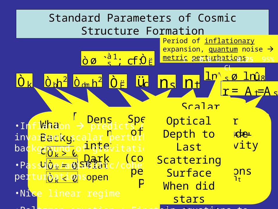
Standard Parameters of Cosmic Structure Formation

Òk

What is the Background curvature of the universe?

Òk > 0Òk = 0Òk < 0

closed

flatopen

Òbh2 ÒË nsÒdmh2

Density of Baryonic Matter

Density of non-interacting Dark

Matter

Cosmological Constant

Spectral index of primordial scalar (compressional)

perturbations

PÐ(k) / knsà1

nt

Spectral index of primordial tensor (Gravity Waves)

perturbations

Ph(k) / knt

lnAs ø lnû8

Scalar Amplitude

r = A t=As

Tensor Amplitude

Period of inflationary expansion, quantum noise metric perturbations

•Inflation predicts nearly scale invariant scalar perturbations and background of gravitational waves

•Passive/adiabatic/coherent/gaussian perturbations

•Nice linear regime

•Boltzman equation + Einstein equations to describe the LSS

üc

Optical Depth to Last Scattering

SurfaceWhen did stars

reionize the universe?

òø `à1s ; cf :ÒË r < 0.6 or < 0.25 95% CL

ns = .958 +- .015

(.99 +.02 -.04 with tensor)

r=At / As < 0.28 95% CL

<1.5 +run

dns /dln k = -.060 +- .022

-.10 +- .05 (wmap3+tensors)

As = 22 +- 2 x 10-10

The Parameters of Cosmic Structure FormationThe Parameters of Cosmic Structure FormationCosmic Numerology: astroph/0611198 – our Acbar paper on the basic 7+

WMAP3modified+B03+CBIcombined+Acbar06+LSS (SDSS+2dF) + DASI (incl polarization and weak lensing and tSZ) cf. WMAP3 + x

bh2 = .0226 +- .0006

ch2 = .114 +- .005

= .73 +.02 - .03

h = .707 +- .021

m= .27 + .03 -.02

zreh = 11.4 +- 2.5

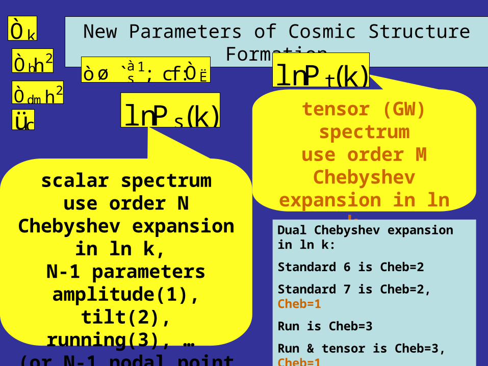
New Parameters of Cosmic Structure FormationÒk

Òbh2

lnP s(k)Òdmh2

scalar spectrumuse order N Chebyshev

expansion in ln k, N-1 parameters

amplitude(1), tilt(2), running(3), …

(or N-1 nodal point k-localized values)

òø `à1s ; cf :ÒË

tensor (GW) spectrumuse order M Chebyshev

expansion in ln k, M-1 parameters amplitude(1), tilt(2),

running(3),...Dual Chebyshev expansion in ln k:

Standard 6 is Cheb=2

Standard 7 is Cheb=2, Cheb=1

Run is Cheb=3

Run & tensor is Cheb=3, Cheb=1

Low order N,M power law but high order Chebyshev is Fourier-like

üc

lnP t(k)

New Parameters of Cosmic Structure FormationÒk

Òbh2lnH(kp)

ï (k); k ù HaÒdmh2

=1+q, the deceleration parameter history

order N Chebyshev expansion, N-1 parameters

(e.g. nodal point values)

P s(k) / H 2=ï ;P t(k) / H 2

òø `à1s ; cf :ÒË

Hubble parameter at inflation at a pivot pt

Fluctuations are from stochastic kicks ~ H/2 superposed on the downward drift at lnk=1.

Potential trajectory from HJ (SB 90,91):

üc

à ï = d lnH =d lna

1à ïà ï = d lnk

d lnH

d lnkd inf = 1à ï

æ ïp

V / H 2(1à 3ï );

ï = (d lnH =d inf)2

H(kp)

tensor (gravity wave) power to curvature power, r, a direct

measure of e = (q+1), q=deceleration parameter during inflation

q (ln Ha) may be highly complex (scanning inflation trajectories)

many inflaton potentials give the same curvature power spectrum, but the degeneracy is broken if gravity waves are measured

Very very difficult to get at with direct gravity wave detectors – even in our dreams (Big Bang Observer ~ 2030)

Response of the CMB photons to the gravitational wave background leads to a unique signature at large angular scales

of these GW and at a detectable level. Detecting these polarization B-modes is the new “holy grail” of CMB science.

Inflation prior: on e only 0 to 1 restriction, < 0 supercritical possible

(q+1) =~ 0 is possible - low energy scale inflation – could get upper limit only on r even with perfect cosmic-variance-limited experiments

GW/scalar curvature: current from CMB+LSS: r < 0.6 or < 0.25 (.28) 95%; good shot at 0.02 95% CL with BB polarization (+- .02 PL2.5+Spider), .01 target

BUT foregrounds/systematics?? But r-spectrum. But low energy inflation

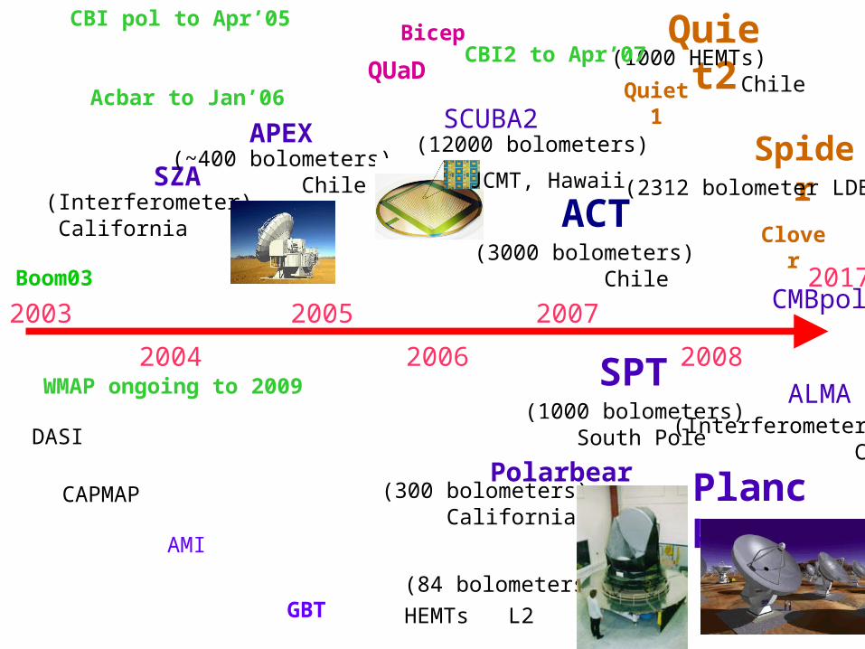
2003

2004

2005

2006

2007

2008

Polarbear(300 bolometers) California

SZA(Interferometer) California

APEX(~400 bolometers) Chile

SPT(1000 bolometers) South Pole

ACT(3000 bolometers) Chile

Planck

(84 bolometers)

HEMTs L2

CMBpol

ALMA(Interferometer) Chile

(12000 bolometers)SCUBA2

Quiet1

Quiet2Bicep

QUaD

CBI pol to Apr’05

Acbar to Jan’06

WMAP ongoing to 2009

2017

(1000 HEMTs) Chile

Spider

Clover

Boom03

DASI

CAPMAP

AMI

GBT

(2312 bolometer LDB)JCMT, Hawaii

CBI2 to Apr’07

CMB/LSS Phenomenology CITA/CIAR here

• Bond

• Contaldi

• Lewis

• Sievers

• Pen

• McDonald

• Majumdar

• Nolta

• Iliev

• Kofman

• Vaudrevange

• Huang

• El Zant

UofT here

• Netterfield

• Carlberg

• Yee

& Exptal/Analysis/Phenomenology Teams here & there

• Boomerang03

• Cosmic Background Imager

• Acbar06

• WMAP (Nolta, Dore)

• CFHTLS – WeakLens

• CFHTLS - Supernovae

• RCS2 (RCS1; Virmos-Descart)

CITA/CIAR there

• Mivelle-Deschenes (IAS)

• Pogosyan (U of Alberta)

• Prunet (IAP)

• Myers (NRAO)

• Holder (McGill)

• Hoekstra (UVictoria)

• van Waerbeke (UBC)

Parameter datasets: CMBall_pol

SDSS P(k), 2dF P(k)

Weak lens (Virmos/RCS1; CFHTLS, RCS2)

Lya forest (SDSS)

SN1a “gold”(157,9 z>1), CFHTLS

futures: ACT SZ/opt, Spider, Planck, 21(1+z)cm

• Dalal

• Dore

• Kesden

• MacTavish

• Pfrommer

• Shirokov

• Dalal

• Dore

• Kesden

• MacTavish

• Pfrommer

• Shirokov

ProkushkinProkushkin

Current state

November 06

Current state

November 06

CBI2 “bigdish” upgrade June2006 + GBT for sourcesCaltech, NRAO, Oxford, CITA, Imperial by about Apr07Caltech, NRAO, Oxford, CITA, Imperial by about Apr07

SZE SZE SecondarySecondary

CMB CMB PrimaryPrimary

on the excess as SZ; (Acbar07); SZA, APEX, ACT, SPT will also nail it

87

8primary

8SZ

astroph/0611198WMAP3’+B03+cbi+acbar03+bima

Std 6 + 8SZ^7σ8 CMBall = 0.78±0.04= 0.92±0.06 SZ

(m = 0.244±0.031)

( = 0.091±0.003)CMBall+LSS = 0.81±0.03 = 0.90±0.06 SZ

(m = 0.274±0.026)

( = 0.090±0.0026)

82

CFHTLS lensing’05: 0.86 +- .05 + Virmos-

Descart & non-G

errors s8 = 0.80

+- .04 if m = 0.3

+- .05

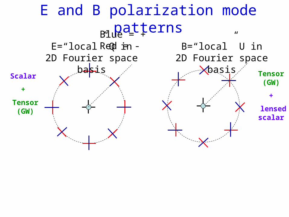
E and B polarization mode patternsBlue = + Red = -

E=“local” Q in 2D Fourier space basis

B=“local” U in 2D Fourier space basis

Tensor (GW)

+

lensed scalar

Scalar

+

Tensor (GW)

Current state

October 06

You are seeing this before people in the

field

Current state

October 06

You are seeing this before people in the

field

Current state

October 06

Polarization

a Frontier

Current state

October 06

Polarization

a Frontier

WMAP3 V band

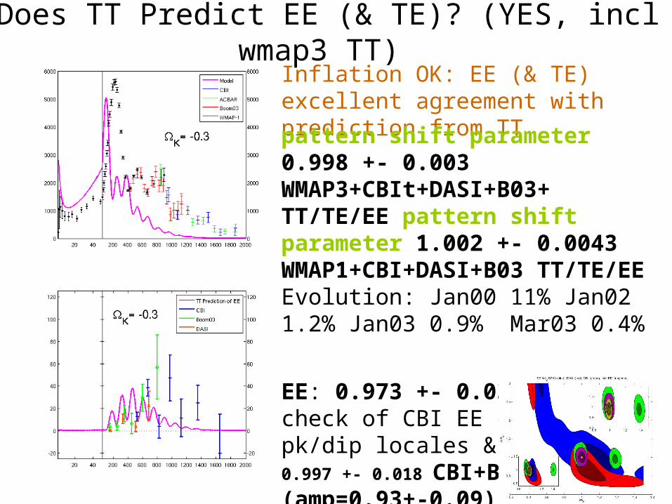
Does TT Predict EE (& TE)? (YES, incl wmap3 TT) Inflation OK: EE (& TE) excellent agreement with prediction from TT

pattern shift parameter 0.998 +- 0.003 WMAP3+CBIt+DASI+B03+ TT/TE/EE pattern shift parameter 1.002 +- 0.0043 WMAP1+CBI+DASI+B03 TT/TE/EE Evolution: Jan00 11% Jan02 1.2% Jan03 0.9% Mar03 0.4%

EE: 0.973 +- 0.033, phase check of CBI EE cf. TT pk/dip locales & amp EE+TE

0.997 +- 0.018 CBI+B03+DASI (amp=0.93+-0.09)

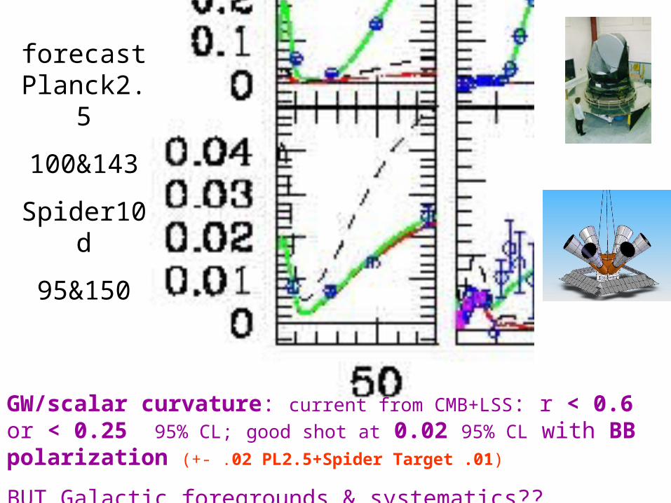
forecast Planck2.5

100&143

Spider10d

95&150

Synchrotron pol’n

< .004 ??

Dust pol’n

< 0.1 ??

Foreground Template removals

from multi-frequency data

forecast Planck2.5

100&143

Spider10d

95&150

GW/scalar curvature: current from CMB+LSS: r < 0.6 or < 0.25 95% CL; good shot at 0.02 95% CL with BB polarization (+- .02 PL2.5+Spider Target .01)

BUT Galactic foregrounds & systematics??

http://www.astro.caltech.edu/~lgg/spider_front.htmhttp://www.astro.caltech.edu/~lgg/spider_front.htm

No Tensor

SPIDER Tensor Signal

Tensor

• Simulation of large scale polarization signal

Inflation Then Trajectories & Primordial Power

Spectrum Constraints

Constraining Inflaton Acceleration Trajectories Bond, Contaldi, Kofman & Vaudrevange 06

Ensemble of Kahler Moduli/Axion InflationsBond, Kofman, Prokushkin & Vaudrevange 06

Constraining Inflaton Acceleration Trajectories Bond, Contaldi, Kofman & Vaudrevange 06

“path integral” over probability landscape of theory and data, with mode-function expansions of the paths truncated by an imposed smoothness

(Chebyshev-filter) criterion [data cannot constrain high ln k frequencies]

P(trajectory|data, th) ~ P(lnHp,k|data, th)

~ P(data| lnHp,k ) P(lnHp,k | th) / P(data|th)

Likelihood theory prior / evidence

“path integral” over probability landscape of theory and data, with mode-function expansions of the paths truncated by an imposed smoothness

(Chebyshev-filter) criterion [data cannot constrain high ln k frequencies]

P(trajectory|data, th) ~ P(lnHp,k|data, th)

~ P(data| lnHp,k ) P(lnHp,k | th) / P(data|th)

Likelihood theory prior / evidence

Data:

CMBall

(WMAP3,B03,CBI, ACBAR,

DASI,VSA,MAXIMA)

+

LSS (2dF, SDSS, 8[lens])

Data:

CMBall

(WMAP3,B03,CBI, ACBAR,

DASI,VSA,MAXIMA)

+

LSS (2dF, SDSS, 8[lens])

Theory prior

uniform in lnHp,k

(equal a-prior probability hypothesis)

Nodal points cf. Chebyshev coefficients (linear

combinations)

monotonic in k

The theory prior matters alot

We have tried many theory priors

Theory prior

uniform in lnHp,k

(equal a-prior probability hypothesis)

Nodal points cf. Chebyshev coefficients (linear

combinations)

monotonic in k

The theory prior matters alot

We have tried many theory priors

Old view: Theory prior = delta function of THE correct one and only theoryOld view: Theory prior = delta function of THE correct one and only theory

New view: Theory prior = probability distribution on an energy landscape whose features are at best only glimpsed, huge number of potential

minima, inflation the late stage flow in the low energy structure toward these minima. Critical role of collective geometrical coordinates (moduli

fields) and of brane and antibrane “moduli” (D3,D7).

New view: Theory prior = probability distribution on an energy landscape whose features are at best only glimpsed, huge number of potential

minima, inflation the late stage flow in the low energy structure toward these minima. Critical role of collective geometrical coordinates (moduli

fields) and of brane and antibrane “moduli” (D3,D7).

lnPs Pt (nodal 2 and 1) + 4 params cf Ps Pt (nodal 5 and 5) + 4 params

reconstructed from CMB+LSS data using Chebyshev nodal point expansion & MCMC

lnPs Pt (nodal 2 and 1) + 4 params cf Ps Pt (nodal 5 and 5) + 4 params

reconstructed from CMB+LSS data using Chebyshev nodal point expansion & MCMC

no self consistency: order 5 in scalar and tensor power

r = .21+- .17 (<.53)

Power law scalar and constant tensor + 4 params

effective r-prior makes the limit stringent

r = .082+- .08 (<.22)

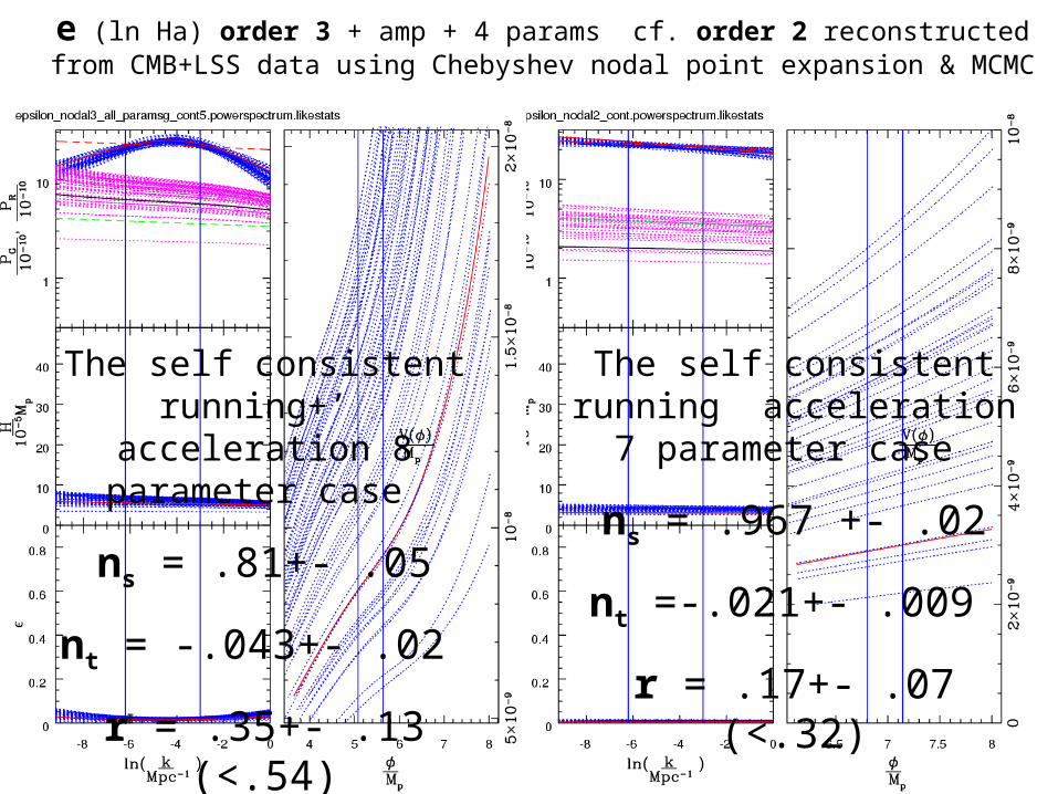
e (ln Ha) order 3 + amp + 4 params cf. order 2 reconstructed from CMB+LSS data using Chebyshev nodal point expansion & MCMC

e (ln Ha) order 3 + amp + 4 params cf. order 2 reconstructed from CMB+LSS data using Chebyshev nodal point expansion & MCMC

The self consistent running+’ acceleration 8 parameter case

ns = .81+- .05

nt = -.043+- .02

r = .35+- .13 (<.54)

The self consistent running acceleration 7 parameter case

ns = .967 +- .02

nt =-.021+- .009

r = .17+- .07 (<.32)

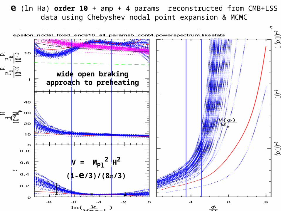
e (ln Ha) order 10 + amp + 4 params reconstructed from CMB+LSS data using Chebyshev nodal point expansion & MCMC

e (ln Ha) order 10 + amp + 4 params reconstructed from CMB+LSS data using Chebyshev nodal point expansion & MCMC

V = MPl2 H2 (1-e/3)/(8/3)V = MPl2 H2 (1-e/3)/(8/3)

wide open braking approach to preheating

wide open braking approach to preheating

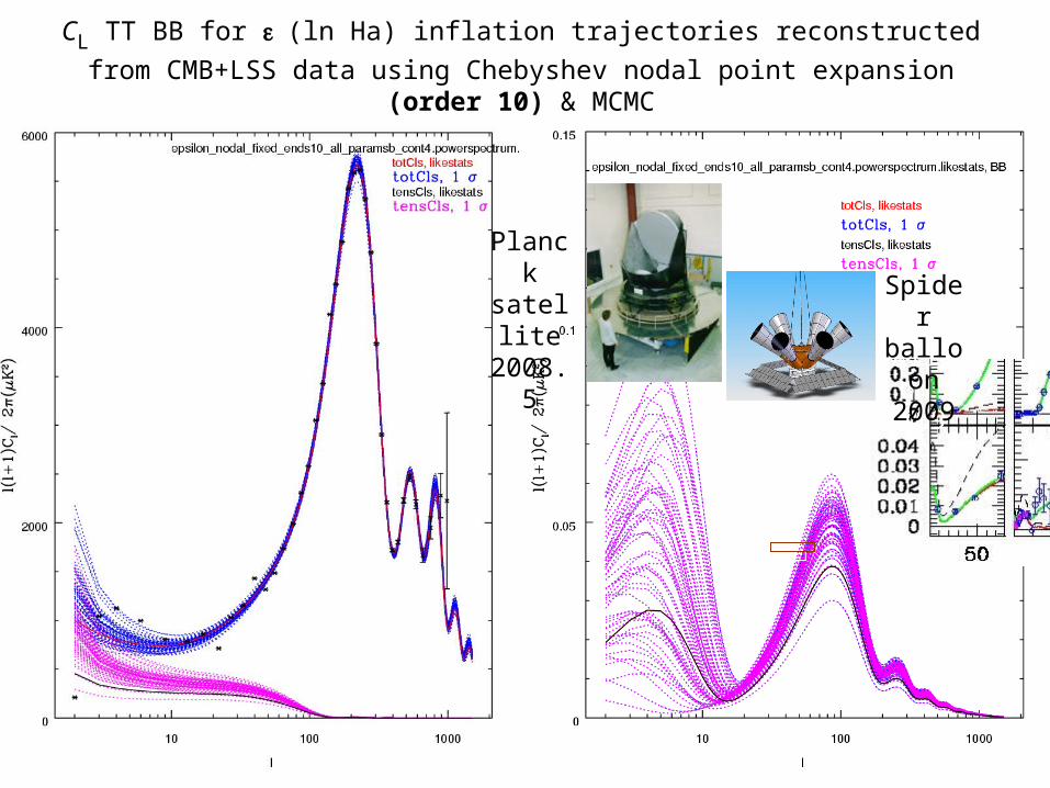
CL TT BB for (ln Ha) inflation trajectories reconstructed from CMB+LSS data

using Chebyshev nodal point expansion (order 10) & MCMC

CL TT BB for (ln Ha) inflation trajectories reconstructed from CMB+LSS data

using Chebyshev nodal point expansion (order 10) & MCMC

Planck satellite 2008.5 Spider

balloon 2009

Spider balloon 2009

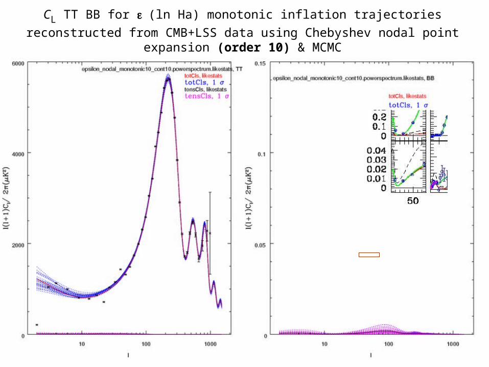
CL TT BB for (ln Ha) monotonic inflation trajectories reconstructed from

CMB+LSS data using Chebyshev nodal point expansion (order 10) & MCMC

CL TT BB for (ln Ha) monotonic inflation trajectories reconstructed from

CMB+LSS data using Chebyshev nodal point expansion (order 10) & MCMC

Inflation in the context of ever changing fundamental theory

1980

2000

1990

-inflation Old Inflation

New Inflation Chaotic inflation

Double InflationExtended inflation

DBI inflation

Super-natural Inflation

Hybrid inflation

SUGRA inflation

SUSY F-term inflation SUSY D-term

inflation

SUSY P-term inflation

Brane inflation

K-flationN-flation

Warped Brane inflation

inflation

Power-law inflation

Tachyon inflationRacetrack inflation

Assisted inflation

Kahler moduli/axion inflation

Natural inflation

String Theory Landscape & Inflation++ Phenomenology for CMB+LSS

Potential of the Hybrid D3/D7 Inflation Model

KKLT, KKLMMTf||

fperp

•D3/anti-D3 branes in a warped geometry

•D3/D7 branes

•axion/moduli fields ...

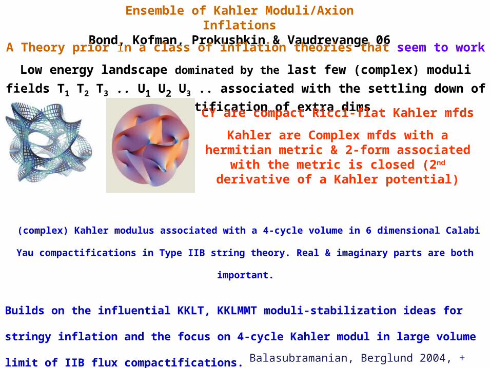
Ensemble of Kahler Moduli/Axion InflationsBond, Kofman, Prokushkin & Vaudrevange 06

A Theory prior in a class of inflation theories that seem to work

Low energy landscape dominated by the last few (complex) moduli fields T1 T2 T3 ..

U1 U2 U3 .. associated with the settling down of the compactification of extra dims

(complex) Kahler modulus associated with a 4-cycle volume in 6 dimensional Calabi Yau

compactifications in Type IIB string theory. Real & imaginary parts are both important.

Builds on the influential KKLT, KKLMMT moduli-stabilization ideas for stringy inflation and the

focus on 4-cycle Kahler modul in large volume limit of IIB flux compactifications. Balasubramanian,

Berglund 2004, + Conlon, Quevedo 2005, + Suruliz 2005 As motivated as any stringy inflation model. Many

possibilities:

Theory prior ~ probability of trajectories given potential parameters of

the collective coordinates X probability of the potential parameters X

probability of initial conditions

CY are compact Ricci-flat Kahler mfds

Kahler are Complex mfds with a hermitian metric & 2-form associated with the metric is closed (2nd derivative of a Kahler potential)

String Theory Landscape & Inflation++ Phenomenology for CMB+LSS

D3/anti-D3 branes in a warped geometry; D3/D7 branes; axion/moduli fields ...

moduli fields dilaton and complex structure moduli stabilized with fluxes in IIB string theory KKLT: volume of CY is stabilized by non-perturbative effects: euclidean D3 brane instanton or gaugino condensate on D7 worldvolume.

T1=1+i1 T2=2+i2 … (axion) gives a rich range of possible potentials & inflation trajectories given

the potential overall scale1

hole scales 2 3

Brane inflation models: highly fine-tuned to avoid heavy inflaton problem (“η-problem”) (D3/anti-D3 KLMMT). most supergravity models also suffer

Brane inflation models: highly fine-tuned to avoid heavy inflaton problem (“η-problem”) (D3/anti-D3 KLMMT). most supergravity models also suffer

Kähler moduli of type IIB string theory compactification on a Calabi-Yau (CY) manifold, weak breaking of Goldstone-boson nature by other non-perturbative effects lifting the potential

Kähler moduli of type IIB string theory compactification on a Calabi-Yau (CY) manifold, weak breaking of Goldstone-boson nature by other non-perturbative effects lifting the potential

Multi-Kahler moduli potential

Multi-Kahler moduli potential

Need at least 2 to stabilize volume (T1 & T3,…) while Kahler-driven T2-inflation occurs, and an uplift to avoid a cosmological constant problem

Need at least 2 to stabilize volume (T1 & T3,…) while Kahler-driven T2-inflation occurs, and an uplift to avoid a cosmological constant problem

T2-TrajectoriesT2-Trajectories

“quantum eternal

inflation” regime

stochastic kick >

classical drift

Sample Kahler modulus potentialSample Kahler modulus potential

Sample trajectories in a Kahler

modulus potential

vs

T=+i

Fixed

Sample trajectories in a Kahler

modulus potential

vs

T=+i

Fixed

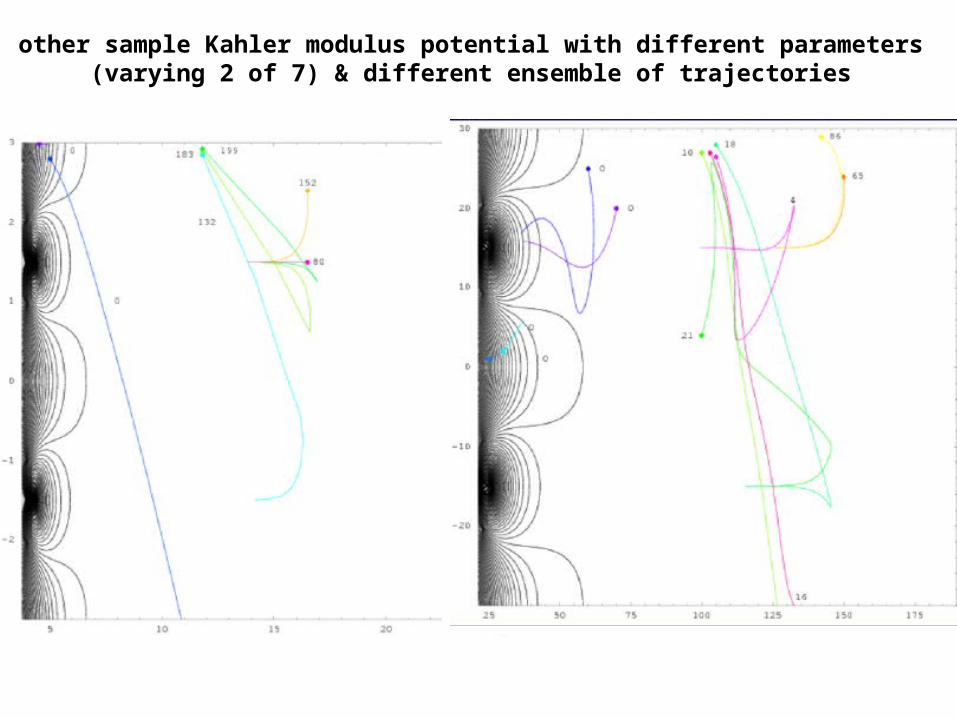
other sample Kahler modulus potential with different parameters (varying 2 of 7) & different ensemble of trajectories

other sample Kahler modulus potential with different parameters (varying 2 of 7) & different ensemble of trajectories

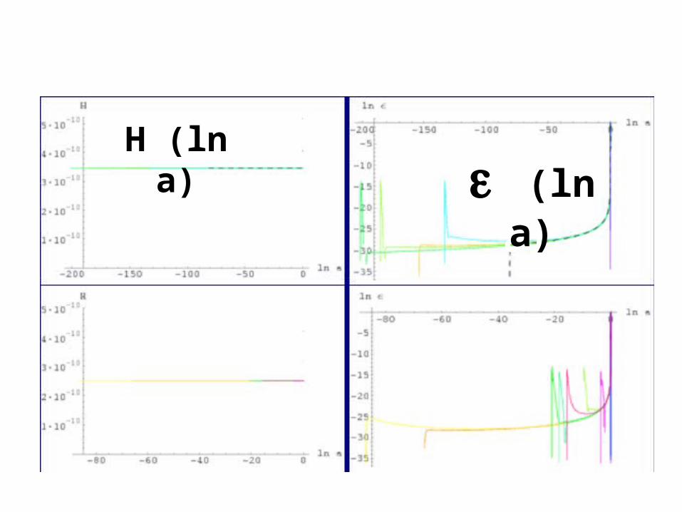
(ln a) (ln a)H (ln a)H (ln a)

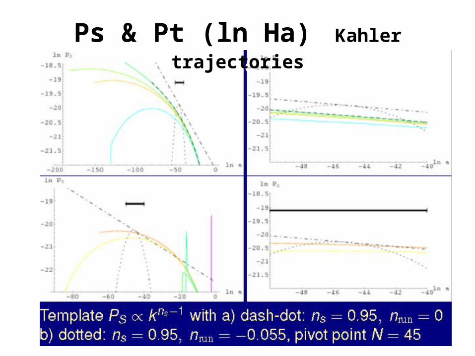
Ps & Pt (ln Ha) Kahler trajectoriesPs & Pt (ln Ha) Kahler trajectories

another example: the axionic freedom complicates scalar

power spectra TBD

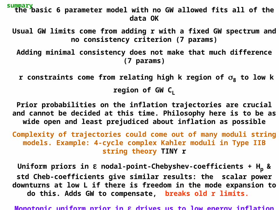
summarysummarythe basic 6 parameter model with no GW allowed fits all of the data OK

Usual GW limits come from adding r with a fixed GW spectrum and no consistency criterion (7 params)

Adding minimal consistency does not make that much difference (7 params)

r constraints come from relating high k region of 8 to low k region of GW CL

Prior probabilities on the inflation trajectories are crucial and cannot be decided at this time. Philosophy here is to be as wide open and least

prejudiced about inflation as possible

Complexity of trajectories could come out of many moduli string models. Example: 4-cycle complex Kahler moduli in Type IIB string theory TINY r

Uniform priors in nodal-point-Chebyshev-coefficients + Hp & std Cheb-

coefficients give similar results: the scalar power downturns at low L if there is freedom in the mode expansion to do this. Adds GW to compensate, breaks

old r limits.

Monotonic uniform prior in drives us to low energy inflation and low gravity wave content.

Even with low energy inflation, the prospects are good with Spider and even Planck to detect the GW-induced B-mode of polarization. Both experiments

have strong Canadian roles (CSA).

End End