CONSTRAINED OPTIMIZATION 2: SQP AND GRG 1 Introduction · The necessary conditions for a...

Chapter 7: Constrained Optimization 2

1

CHAPTER 7

CONSTRAINED OPTIMIZATION 2: SQP AND GRG

1 Introduction

In the previous chapter we examined the necessary and sufficient conditions for a constrained optimum. We did not, however, discuss any algorithms for constrained optimization. That is the purpose of this chapter. In an oft referenced study done in 19801, dozens of nonlinear algorithms were tested on roughly 100 different nonlinear problems. The top-ranked algorithm was SQP. Of the five top algorithms, two were SQP and three were GRG. Although many different algorithms have been proposed, based on these results, we will study only these two. SQP works by solving for where the KT equations are satisfied. SQP is a very efficient algorithm in terms of the number of function calls needed to get to the optimum. It converges to the optimum by simultaneously improving the objective and tightening feasibility of the constraints. Only the optimal design is guaranteed to be feasible; intermediate designs may be infeasible. The GRG algorithm works by computing search directions which improve the objective and satisfy the constraints, and then conducting line searches in a very similar fashion to the algorithms we studied in Chapter 3. GRG requires more function evaluations than SQP, but it has the desirable property that it stays feasible once a feasible point is found. If the optimization process is halted before the optimum is reached, the designer is guaranteed to have in hand a better design than the starting design. GRG also appears to be more robust (able to solve a wider variety of problems) than SQP, so for engineering problems it is often the algorithm tried first.

2 The Sequential Quadratic Programming (SQP) Algorithm

The SQP algorithm was developed in the early 1980’s by M. J. D. Powell, a mathematician at Cambridge University. Before we begin describing this algorithm, we need to present some background information.

2.1 The Newton Raphson Method for Solving Nonlinear Equations

If we were to sum up how the SQP methods works in one sentence it would be: the SQP algorithm applies the Newton-Raphson method to solve the Kuhn-Tucker equations. Or, in short, SQP does N-R on the K-T! Thus we will begin by reviewing how the Newton Raphson method works.

1 Schittkowski, K., "Nonlinear Programming codes: Information, Tests, Performance," Lecture Notes in Economics and Mathematical Systems, vol. 183, Springer-Verlag, New York, 1980.


2

2.1.1 One equation with One Unknown

The N-R method is used to find the solution to sets of nonlinear equations. For example, suppose we wish to find the solution to the equation: 2 xx e We cannot solve for x directly. The N-R method solves the equation in an iterative fashion based on results derived from the Taylor expansion. First, the equation is rewritten in the form, 2 0xx e (7.1) We then provide a starting estimate of the value of x that solves the equation. This point becomes the point of expansion for a Taylor series:

0

0 0dFF F x x

dx (7.2)

(For reasons that will become apparent later, we will use F instead of f for our functions here.) We would like to drive the value of the function to zero:

0

0 00 - dF

F x xdx

(7.3)

If we denote 0x x x , and solve for x in (7.3):

0

/

Fx

dF dx

(7.4)

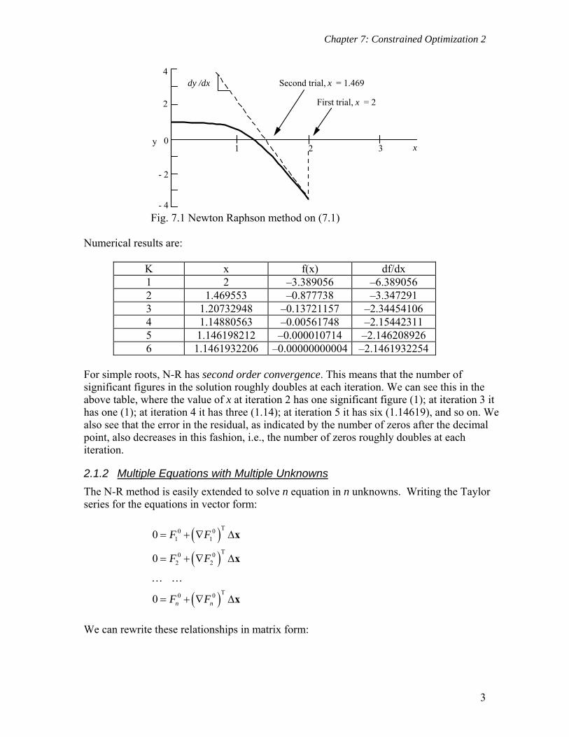
We then add x to 0x to obtain a new guess for the value of x that satisfies the equation, obtain the derivative there, get the new function value, and iterate until the function value or residual, goes to zero. The process is illustrated in Fig. 7.1 for the example given in (7.1), with a starting guess 2.0x .


3

1 2 3 x

Second trial, x = 1.469

First trial, x = 2

dy /dx4

2

y 0

- 2

- 4 Fig. 7.1 Newton Raphson method on (7.1) Numerical results are:

K x f(x) df/dx 1 2 –3.389056 –6.389056 2 1.469553 –0.877738 –3.347291 3 1.20732948 –0.13721157 –2.34454106 4 1.14880563 –0.00561748 –2.15442311 5 1.146198212 –0.000010714 –2.146208926 6 1.1461932206 –0.00000000004 –2.1461932254

For simple roots, N-R has second order convergence. This means that the number of significant figures in the solution roughly doubles at each iteration. We can see this in the above table, where the value of x at iteration 2 has one significant figure (1); at iteration 3 it has one (1); at iteration 4 it has three (1.14); at iteration 5 it has six (1.14619), and so on. We also see that the error in the residual, as indicated by the number of zeros after the decimal point, also decreases in this fashion, i.e., the number of zeros roughly doubles at each iteration.

2.1.2 Multiple Equations with Multiple Unknowns

The N-R method is easily extended to solve n equation in n unknowns. Writing the Taylor series for the equations in vector form:

T0 01 1

T0 02 2

T0 0

0

0

0 n n

F F

F F

F F

x

x

x

We can rewrite these relationships in matrix form:


4

T001

1T 00

22

0T0

nn

FF

FF

FF

x

(7.5)

For 2 X 2 System,

1 1

1 2 1 1

2 22 2

1 2

F F

x x x F

x FF F

x x

(7.6)

In (7.5) we will denote the vector of residuals as 0F . (This violates our notation convention that bold caps represent matrices, not vectors. Just remember that F is a vector, not a matrix.) We will denote the matrix of coefficients as G. Equation (7.5) can then be written, G x F (7.7) The solution is obviously

-1 x G F (7.8)

2.1.3 Using the N-R method to Solve the Necessary Conditions

In this section we will make a very important connection—we will apply N-R to solve the necessary conditions. Consider for example, a very simple case—an unconstrained problem in two variables. We know the necessary conditions are,

1

2

0

0

f

x

f

x

(7.9)

Now suppose we wish to solve these equations using N-R, that is we wish to find x* to drive the partial derivatives of f to zero. In terms of notation and discussion this gets a little tricky because the N-R method involves taking derivatives of the equations to be solved, and the equations we wish to solve are composed of derivatives. So when we substitute (7.9) into the N-R method, we end up with second derivatives.

For example, if we set 1 21 2

andf f

F Fx x

. Then we can write (7.6) as,


5

1 1 2 1 11

2

1 2 2 2 2

f f f

x x x x xx

xf f f

x x x x x

(7.10)

or,

2 2

21 2 1 11

2 22

221 2 2

f f f

x x x xx

x ff fxx x x

(7.11)

which should be familiar from Chapter 3, because (7.11) can be written in vector form as, f H x (7.12) and the solution is,

1 f x H (7.13)

We recognize (7.12-7.13) as Newton’s method for solving for an unconstrained optimum. Thus we have the important result that Newton’s method is the same as applying N-R on the necessary conditions for an unconstrained problem. From the properties of the N-R method, we know that if Newton’s method converges (and recall that it doesn’t always converge), it will do so with second order convergence—which is very fast. Now just to indicate where we are heading, after we introduce the SQP approximation, the next step is to show that the SQP method is the same as doing N-R on the necessary conditions for a constrained problem (with some tweaks to make it efficient and to ensure it converges).

2.2 Constrained Optimization: Equality Constraints

2.2.1 Problem Definition

We will start with a problem which only has equality constraints. We recall that when we only have equality constraints, we do not have to worry about complementary slackness which makes things simpler. So the problem we will focus on is, Min f x (7.14)

st. 0 1, 2, ,i ig b i m x (7.15)


6

The necessary conditions for a constrained optimal solution are:

1

m

i ii

f g

0 (7.16)

0 1, ,i ig b i m (7.17)

2.2.2 The SQP Approximation

As we have previously mentioned in Chapter 6, a problem with a quadratic objective and linear constraints is known as a quadratic programming problem. These problems have a special name because the K-T equations are linear and are easily solved. We will make a quadratic programming approximation at the point 0x to the problem given by (7.14-7.15)

T0 0 T 2 01L

2a xf f f x x x (7.18)

T0 0, 1, ,i a i i ig g g b i m x (7.19)

where the subscript a is used in af to indicate the approximation. Close examination of

(7.18) shows something unexpected. Instead of 2 f as we would normally have if we were

doing a Taylor approximation of the objective, we have 2xL , the Hessian of the Lagrangian

function with respect to x. Why is this case? It is directly tied to applying N-R on the K-T, as we will presently show. For now we will just accept that the objective uses the Hessian of the Lagrangian instead of the Hessian of the objective. We will solve the QP approximation, (7.18-7.19), by solving the K-T equations for this problem, which, as mentioned, are linear. These equations are given by,

,1

m

a i i ai

f g

0 (7.20)

, 0 1, ,i a ig b for i m (7.21)

Since, for example, from (7.18), 0 2 0La xf f x

we can also write these equations in terms of the original problem,

0 2 0 0

1

Lm

x i ii

f g

x 0 (7.22)

T0 0 0 1, ,i i ig g b for i m x (7.23)


7

These are a linear set of equations we can readily solve, as shown in the example in the next section. For Section 2.2.4, we will want to write these equations even more concisely. If we define the following matrices and vectors,

T01

T00 0 0 0 02

1 2

T0

, ,T

m

m

g

gg g g

g

J J

011

020 2 0 2 0 2 02

1

0

Lm

x i ii

mm

bg

bgf g

bg

g b

We can write (7.22-7.23) as,

T2 0 0 0Lx f x J λ (7.24)

0 0 J x g b (7.25)

Again, to emphasize, this set of equations represents the solution to (7.18-7.19).

2.2.3 Example 1: Solving the SQP Approximation

Suppose we have as our approximation the following,

1 11 2

2 2

1

2

1 013 3 2

0 12

5 1 3 0

a

a

x xf x x

x x

xg

x

(7.26)

We can write out the K-T equations for this approximation as,

1

2

1

2

3 1 0 10

2 0 1 3

5 1 3 0

a

a

xf

x

xg

x

(7.27)

We can rewrite these equations in matrix form as,


8

1

2

1 0 1 3

0 1 3 2

1 3 0 5

x

x

(7.28)

The solution is,

1

2

2.6

0.8

0.4

x

x

(7.29)

Observations: This calculation represents the main step in an iteration of the SQP algorithm which solves a sequence of quadratic programs. If we wanted to continue, we would add x to our current x, update the Lagrangian Hessian, make a new approximation, solve for that solution, and continue iterating in this fashion. If we ever reach a point where x goes to zero as we solve for the optimum of the approximation, the original K-T equations are satisfied. We can see this by examining (7.22-7.23). If x is zero, we have,

2 *

10

Lm

x i ii

f g

x 0

(7.30)

T

0

0 1, ,i i ig g b for i m

x

(7.31)

which then match (7.16-7.17).

2.2.4 N-R on the K-T Equations for Problems with Equality Constraints

In this section we wish to look at applying the N-R method to the original K-T equations. The K-T equations for a problem with equality constraints only, as given by (7.16-7.17), are,

1

m

i ii

f g

0 (7.32)

0 1, ,i ig b i m (7.33)

Now suppose we wish to solve these equations using the N-R method. To implement N-R we would have,


9

1 11

1 11 1

T T

x

T T

x n n nTT

x

TT m mx m m

F F F

F F F

g bg g

g bg g

x

λ

(7.34)

where 1F for example, is given by,

111 1

mi

ii

gfF

x x

(7.35)

If we substitute (7.35) into matrix (7.32), the first row becomes,

2 2 22 2 21 2

2 21 1 11 1 2 1 2 1 1 1 1 1 1

, , , , , , ,m m m

i i i mi i i

i i in n

g g g gg gf f f

x x x x x x x x x x x x x

Recalling,

2 2 2

1

m

x i ii

L f g

And using the matrices we defined above,

T01

T00 0 0 0 02

1 2

T0

, ,T

m

m

g

gg g g

g

J J

011

020 2 0 2 0 2 02

1

0

Lm

x i ii

mm

bg

bgf g

bg

g b

we can rewrite (7.34) as,

02 0 0 0 0 0

00 0

L

0 ( )

T T

x f

x xJ J λ

λ λJ g b (7.36)


10

If we do the matrix multiplications we have

T2 0 0 0 0 0 0L ( )T

x f x J λ λ J λ (7.37)

0 0 J x g b

and collecting terms,

T2 0 0 0Lx f x J λ (7.38)

0 0 J x g b

which equations are the same as (7.24-7.25). Thus we see that doing a N-R iteration on the K-T equations is the same as solving for the optimum of the QP approximation. This is the reason we use the Hessian of the Lagrangian function rather than the Hessian of the objective in the approximation.

2.3 Constrained Optimization: Inequality and Equality Constraints

In the previous section we considered equality constraints only. We need to extend these results to the general case. We will state this problem as Min f x

s.t. 0 1, ,i ig b i k x (7.39)

0 1, ,i ig b i k m x

The quadratic approximation at point xo is:

Min T T0 0 2 01L

2a xf f f x x x

s.t. , :i ag 0 0 1, 2,...,T

i i ig g b i k x (7.40)

0 0 1,...,T

i i ig g b i k m x

Notice that the approximations are a function only of ∆x. All gradients and the Lagrangian hessian in (7.40) are evaluated at the point of expansion and so represent known quantities. In the article where Powell describes this algorithm,2 he makes a significant statement at this point. Quoting, “The extension of the Newton iteration to take account of inequality constraints on the variables arises from the fact that the value of x that solves (7.39) can

2 Powell, M.J.D., "A Fast Algorithm for Nonlinearly Constrained Optimization Calculations," Numerical Analysis, Dundee 1977, Lecture Notes in Mathematics no. 630, Springer-Verlag, New York, 1978


11

also be found by solving a quadratic programming problem. Specifically, x is the value that makes the quadratic function in (7.40) stationary.” Further, the value of for the K-T conditions is equal to the vector of Lagrange multipliers of the quadratic programming problem. Thus solving the quadratic objective and linear constraints in (7.40) is the same as solving the N-R iteration on the original K-T equations. The main difficulty in extending SQP to the general problem has to do the with the complementary slackness condition. This equation is non-linear, and so makes the QP problem nonlinear. We recall that complementary slackness basically enforces that either a constraint is binding or the associated Lagrange multiplier is zero. Thus we can incorporate this condition if we can develop a method to determine which inequality constraints are binding at the optimum. An example of a modern solution technique is given by Goldfarb and Idnani.3 This algorithm starts out by solving for the unconstrained optimum to the problem and evaluating which constraints are violated. It then moves to add in these constraints until it is at the optimum. Thus it tends to drive to the optimum from infeasible space. There are other important details to develop a realistic, efficient SQP algorithm. For example, the QP approximation involves the Lagrangian hessian matrix, which involves second derivatives. As you might expect, we don't evaluate the Hessian directly but approximate it using a quasi-Newton update, such as the BFGS update. Recall that updates use differences in x and differences in gradients to estimate second derivatives. To estimate 2Lx we will need to use differences in the gradient of the

Lagrangian function,

1

Lm

x i ii

f g

Note that to evaluate this gradient we need values for i. We will get these from our solution to the QP problem. Since our update stays positive definite, we don’t have to worry about the method diverging, like Newton’s method does for unconstrained problems.

2.4 Comments on the SQP Algorithm

The SQP algorithm has the following characteristics, The algorithm is very fast. It is the most efficient optimization algorithm available

today. Because it does not rely on a traditional line search, it is often more accurate in

identifying an optimum.

3 Goldfarb, D., and A. Idnani, "A Numerically Stable Dual Method for Solving Strictly Convex Quadratic Programs," Math. Programming, v. 27, 1983, p.1-33.


12

The efficiency of the algorithm is partly because it does not enforce feasibility of the constraints at each step. Rather it gradually enforces feasibility as part of the K-T conditions. It is only guaranteed to be feasible at the optimum.

Relative to engineering problems, there are some drawbacks:

Because it can go infeasible during optimization—sometimes by relatively large amounts—it can crash engineering models.

It is more sensitive to numerical noise and/or error in derivatives than GRG. If we terminate the optimization process before the optimum is reached, SQP does

not guarantee that we will have in-hand a better design than we started with. GRG does guarantee this.

2.5 Summary of Steps for SQP Algorithm

1. Make a QP approximation to the original problem. For the first iteration, use a Lagrangian Hessian equal to the identity matrix.

2. Solve for the optimum to the QP problem. As part of this solution, values for the Lagrange multipliers are obtained.

3. Execute a simple line search by first stepping to the optimum of the QP problem. So the

initial step is ∆x, and new old x x x . See if at this point a penalty function, composed of the values of the objective and violated constraints, is reduced. If not, cut back the step size until the penalty function is reduced. The penalty function is given

by1

vio

i ii

P f g

where the summation is done over the set of violated constraints, and

the absolute values of the constraints are taken. The Lagrange multipliers act as scaling or weighting factors between the objective and violated constraints.

4. Evaluate the Lagrangian gradient at the new point. Calculate the difference in x and in the Lagrangrian gradient, . Update the Lagrangian Hessian using the BFGS update.

5. Return to Step 1 until ∆x is sufficiently small. When ∆x approaches zero, the K-T

conditions for the original problem are satisfied.

2.6 Example of SQP Algorithm

Find the optimum to the problem, Min 4 2 2 2

1 2 1 2 1 12 2 5f x x x x x x x

s.t. 2

1 20.25 0.75 0g x x x

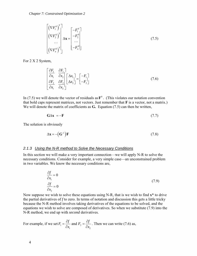
starting from the point -1,4 . A contour plot of the problem is shown in Fig. 7.2. This

problem is interesting for several reasons: the objective is quite eccentric at the optimum, the algorithm starts at point where the search direction is pointing away from the optimum, and the constraint boundary at the starting point has a slope opposite to that at the optimum.


13

Fig. 7.2. Contour plot of example problem for SQP algorithm.

Iteration 1 We calculate the gradients, etc. at the beginning point. The Lagrangian Hessian is initialized to the identity matrix.

At T0 0 0 2 0 1 0-1,4 , 17, 8,6 , L

0 1

Tf f

x

0 02.4375, 1.5, 0.75T

g g

Based on these values, we create the first approximation,

1 11 2

2 2

1 0117.0 8 6

0 12a

x xf x x

x x

1

2

2.4375 1.5 0.75 0a

xg

x

We will assume the constraint is binding. Then the K-T conditions for the optimum of the approximation are given by the following equations: 0a af g

0ag


14

These equations can be written as, 18 1.5 0x

26 0.75 0x

1 22.4375 1.5 0.75 0x x

The solution to this set of equations is 1 20.5, 2.25, 5.00x x

The proposed step is, 1 0 1 0.5 1.5

4 2.25 1.75

x x x

Before we accept this step, however, we need to check the penalty function,

1

vio

i ii

P f g

to make sure it decreased with the step. At the starting point, the constraint is satisfied, so the penalty function is just the value of the objective, 17P . At the proposed point the objective value is 10.5f and the constraint is slightly violated with 0.25g . The penalty

function is therefore, 10.5 5.0* 0.25 11.75P . Since this is less than 17, we accept the

full step. Contours of the first approximation and the path of the first step are shown in Fig. 7.3.

Fig. 7.3 The first SQP approximation and step.


15

Iteration 2

At T1 1 11.5 1.75 , 10.5, 8.0 1.0 ,T

f f x

1 10.25, 2.5 0.75T

g g

We now need to update the Hessian of the Lagrangian. To do this we need the Lagrangian gradient at x0 and x1. (Note that we use the same Lagrange multiplier, 1 , for both gradients.)

0 1 8.0 1.5 0.5L , 5.0

6.0 0.75 2.25

x λ

1 1 8.0 2.5 20.5L , 5.0

1.0 0.75 4.75

x λ

0 1 1 0 1 21.0L , L ,

7.0

γ x λ x λ

0 1.5 1.0 0.5

1.75 4.0 2.25

x

From Chapter 3, we will use the BFGS Hessian update,

T T

1T T

k k k k k k

k k

k k k k k

γ γ H x x HH H

γ x x H x

Substituting:

2 1

21.0 1. 0. 0.5 1. 0.21.0 7.0 0.5 2.25

1. 0. 7.0 0. 1. 2.25 0. 1.L

0.5 1. 0. 0.50. 1.21.0 7.0 0.5 2.25

2.25 0. 1. 2.25

2 1 1. 0. 16.8000 5.6000 0.0471 0.2118L

0. 1. 5.6000 1.8667 0.2118 0.9529

2 1 17.7529 5.3882L

5.3882 1.9137


16

The second approximation is therefore,

1 11 2

2 2

17.753 5.3882110.5 8.0 1.0

5.3882 1.91372a

x xf x x

x x

1

2

0.25 2.5 0.75 0a

xg

x

As we did before, we will assume the constraint is binding. The K-T equations are, 1 28 17.753 5.3882 2.5 0x x

1 21 5.3882 1.9137 0.75 0x x

1 20.25 2.5 0.75 0x x

The solution to this set of equations is 1 21.6145, 5.048, 2.615x x . Because is

negative, we need to drop the constraint from the picture. (We can see in Fig. 7.4 below that the constraint is not binding at the optimum.) With the constraint dropped, the solution is, 1 22.007, 5.131, 0.x x This gives a new x of,

2 1 1.5 2.007 0.507

1.75 5.131 3.381

x x x

However, when we try to step this far, we find the penalty function has increased from 11.75 to 17.48 (this is the value of the objective only—the violated constraint does not enter in to the penalty function because the Lagrange multiplier is zero). We cut the step back. How much to cut back is somewhat arbitrary. We will make the step 0.5 times the original. The new value of x becomes,

2 1 1.5 2.007 0.49650.5

1.75 5.131 0.8155

x x x

At which point the penalty function is 7.37. So we accept this step. Contours of the second approximation are shown in Fig. 7.4, along with the step taken.


17

Fig. 7.4 The second approximation and step.

Iteration 3

At T2 2 20.4965 0.8155 , 7.367, 5.102 2.124 ,T

f f x

2 20.6724, 0.493 0.75T

g g

1 2 8.0 2.5 8.0L , 0

1.0 0.75 1.0

x λ

2 2 5.102 0.493 5.102L , 0

2.124 0.75 2.124

x λ

1 2 2 1 2 2.898L , L ,

1.124

γ x λ x λ

1 0.4965 1.5 1.004

0.8155 1.75 2.5655

x

Based on these vectors, the new Lagrangian Hessian is,

2 2 17.7529 5.3882 1.4497 0.5623 5.8551 0.7320L

5.3882 1.9137 0.5623 0.2181 0.7320 0.0915


18

2 2 13.3475 4.0939L

4.0939 2.0403

So our next approximation is,

1 11 2

2 2

13.3475 4.093917.367 5.102 2.124

4.0939 2.04032a

x xf x x

x x

1

2

0.6724 0.493 0.75 0a

xg

x

The K-T equations, assuming the constraint is binding, are, 1 25.102 13.3475 4.0939 0.493 0x x

1 22.124 4.0939 2.0403 0.75 0x x

1 20.6724 0.493 0.75 0x x

The solution to this set of equations is 1 20.1399, 0.8046, 0.1205x x .

Our new proposed point is, 3 2 0.4965 0.1399 0.3566

0.8155 0.8046 0.0109

x x x

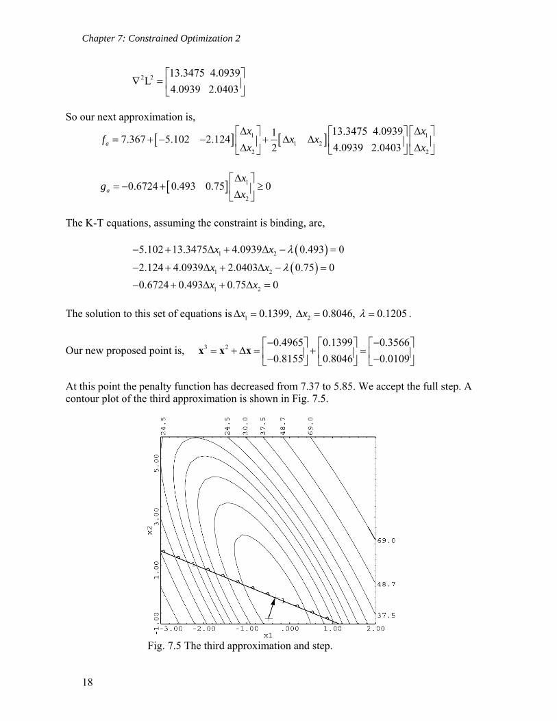
At this point the penalty function has decreased from 7.37 to 5.85. We accept the full step. A contour plot of the third approximation is shown in Fig. 7.5.

Fig. 7.5 The third approximation and step.


19

Iteration 4

At 3 3 30.3566 0.0109 , 5.859, 2.9101 0.2761 ,T T

f f x

3 30.01954, 0.2132 0.75T

g g

2 3 5.102 0.493 5.161L , 0.1205

2.124 0.75 2.214

x λ

3 3 2.910 0.2132 2.936L , 0.1205

0.2761 0.75 0.3665

x λ

2 3 3 2 3 2.225L , L ,

1.8475

γ x λ x λ

2 0.3566 0.4965 0.1399

0.0109 0.8155 0.8046

x


2 3 13.3475 4.0939 2.7537 2.2865 10.6397 4.5647L

4.0939 2.0403 2.2865 1.8986 4.5647 1.9584

2 3 5.4616 1.8157L

1.8157 1.9805

Our new approximation is,

1 11 2

2 2

5.4616 1.815715.859 2.910 0.2761

1.8157 1.98052a

x xf x x

x x

1

2

0.0195 0.2132 0.75 0a

xg

x

The K-T equations, assuming the constraint is binding, are, 1 22.910 5.4616 1.8157 (0.2132) 0x x

1 20.2761 1.8157 1.9805 0.75 0x x

1 20.0195 0.2132 0.75 0x x


20

The solution to this problem is, 1 20.6099, 0.1474, 0.7192x x . Since is

positive, our assumption about the constraint was correct. Our new proposed point is,

4 3 0.3566 0.6099 0.2533

0.0109 0.1474 0.1583

x x x

At this point the penalty function is 4.87, a decrease from 5.85, so we take the full step. The contour plot is given in Fig. 7.6

Fig. 7.6 The fourth approximation and step.

Iteration 5

At 4 4 40.2533 0.1583 , 4.6071, 1.268 0.4449 ,T T

f f x

4 40.3724, 1.007 0.75T

g g

3 4 2.9101 0.2132 3.063L , 0.7192

0.2761 0.75 0.8155

x λ

4 4 1.268 1.007 0.5438L , 0.7192

0.4449 0.75 0.9843

x λ

3 4 4 3 4 2.519L , L ,

0.1688

γ x λ x λ


21

3 0.2533 0.3566 0.6099

0.1583 0.0109 0.1474

x


2 4 5.4616 1.8157 4.0644 0.2724 5.3681 1.4290L

1.8157 1.9805 0.2724 0.0183 1.4290 0.3804

2 4 4.1578 0.1144L

0.1144 1.6184

Our new approximation is,

1 11 2

2 2

4.1578 0.114414.6071 1.268 0.4449

0.1144 1.61842a

x xf x x

x x

1

2

0.3724 -1.007 0.75 0a

xg

x

The K-T equations, assuming the constraint is binding, are, 1 21.268 4.1578 0.1144 ( 1.007) 0x x

1 20.4449 0.1144 1.6184 0.75 0x x

1 20.3724 1.007 0.75 0x x

The solution to this problem is, 1 20.0988, 0.6292, 0.7797x x . Since is positive,

our assumption about the constraint was correct. Our new proposed point is,

5 4 0.2533 0.0988 0.3521

0.1583 0.6292 0.4709

x x x

At this point the penalty function is 4.55, a decrease from 4.87, so we take the full step. The contour plot is given in Fig. 7.7 We would continue in this fashion until x goes to zero. We would then know the original K-T equations were satisfied. The solution to this problem occurs at,

T* *0.495 0.739 , 4.50f x

Using OptdesX, SQP requires 25 calls to the analysis program. GRG takes 50 calls.


22

Fig. 7.7 The fifth approximation and step.

A summary of all the steps is overlaid on the original problem in Fig. 7.8.

Fig. 7.8 The path of the SQP algorithm.


23

3 The Generalized Reduced Gradient (GRG) Algorithm

3.1 Introduction

In the previous section we learned that SQP works by solving for the point where the K-T equations are satisfied. SQP gradually enforces feasibility of the constraints as part of the K-T equations. In this section we will learn how GRG works. We will find it is very different from SQP. If started inside feasible space, GRG goes downhill until it runs into fences—constraints--and then corrects the search direction such that it follows the fences downhill. At every step it enforces feasibility. The strategy of GRG in following fences works well for engineering problems because most engineering optimums are constrained.

3.2 Explicit vs. Implicit Elimination

Suppose we have the following optimization problem, Min 2 2

1 23f x x x (7.41)

s.t. 1 22 6 0g x x x (7.42)

A contour plot is given in Fig. 7.9a. From previous discussions about modeling in Chapter 2, we know there are two approaches to this problem—we can solve it as a problem in two variables with one equality constraint, or we can use the equality constraint to eliminate a variable and the constraint. We will use the second approach. Using (7.42) to solve for 2x ,

2 16 2x x

Substituting into the objective function, (7.41), we have, Min 2 2

1 13(6 2 )f x x x (7.43)

Mathematically, solving the problem given by (7.41-7.42) is the same as solving the problem in (7.43). We have used the constraint to explicitly eliminate a variable and a constraint. Once we solve for the optimal value of 1x , we will obviously have to back substitute to get

the value of 2x using 7.42. The solution in 1x is illustrated in Fig. 7.9b, where the sensitivity

plot for 7.43 is given (because we only have one variable, we can’t show a contour plot). The

derivative 1

df

dxof (7.43) would be considered to be the reduced gradient relative to the

original problem.


24

Usually we cannot make an explicit substitution as we did in this example. So we eliminate variables implicitly. We show how this can be done in the next section.

Fig. 7.9 a) Contour plot in 1 2,x x with equality

constraint. The optimum is at

2.7693 0.4613T x .

Fig. 7.9 b) Sensitivity plot for 7.43. The optimum is at 1 2.7693x

3.3 Implicit Elimination

In this section we will look at how we can eliminate variables implicitly. We do this by considering differential changes in the objective and constraints. We will start by considering a simple problem of two variables with one equality constraint, Min 1 2

Tf x xx x (7.44)

s.t. 0g b x (7.45)

Suppose we are at a feasible point. Thus the equality constraint is satisfied. We wish to move to improve the objective function. The differential change is given by,

1 21 2

f fdf dx dx

x x

(7.46)

to keep the constraint satisfied the differential change must be zero:

1 21 2

0g g

dg dx dxx x

(7.47)

Solving for 2dx in (7.47) gives:


25

12 1

2

g xdx dx

g x

substituting into (7.46) gives,

11

1 2 2

f f g xdf dx

x x g x

(7.48)

where the term in brackets is the reduced gradient.

i.e., 1

1 1 2 2

Rdf f f g x

dx x x g x

(7.49)

If we substitute x for dx , then the equations are only approximate. We are stepping tangent to the constraint in a direction that improves the objective function.

3.4 GRG Algorithm with Equality Constraints Only

We can extend the concepts of the previous section to the general problem which we represent in vector notation. Suppose now we consider the general problem with equality constraints, Min f x

s.t. 0 1, ,i ig b i m x

We have n design variables and m equality constraints. We begin by partitioning the design variables into (n-m) independent variables, z, and m dependent variables y. The independent variables will be used to improve the objective function, and the dependent variables will be used to satisfy the binding constraints. If we partition the gradient vectors as well we have,

T

1 2 n m

f f ff

z z z

x x xz

T

1 1 m

f f ff

y y y

x x xy

We will also define independent and dependent matrices of the partial derivatives of the constraints:

1 1 1

1 2

1 2

n m

m m m

n m

g g g

z z z

g g g

z z z

z

1 1

1 2

1 2

m

m

m m m

m

gg g

y y y

g g g

y y y

y


26

We can write the differential changes in the objective and constraints in vector form as:

T Tdf f d f d z z y y (7.50)

d d d

z y 0z y

(7.51)

Noting that y

is a square matrix, and solving (7.51) for dy,

1

d d

y zy z

(7.52)

substituting (7.52) into (7.50),

1

T Tdf f d f d

z z y z

y z

or 1

T TTRf f f

z y

y z (7.53)

where T

Rf is the reduced gradient. The reduced gradient is the direction of steepest ascent

that stays tangent to the binding constraints.

3.5 GRG Example 1: One Equality Constraint

We will illustrate the theory of the previous section with the following example. For this example we will have three variables and one equality constraint. We state the problem as, Min 2 2 2

1 2 34 3f x x x

s.t. 1 2 32 4 10g x x x

Step 1: Evaluate the objective and constraints at the starting point. The starting point will be 2 2 2T x , at which point 32 and 10f g . So the

constraint is satisfied. Step 2: Partition the variables. We have one binding constraint so we will need one dependent variable. We will arbitrarily choose 1x as the dependent variable, so 1xy . The independent variables will therefore be

2 3T x xz . Thus,


27

22 21 1 @2

3 3 1@2,2

3

2 48 16

6 12

f

xx x fx f f x

x xf x

x

z y z y

2 3 1

4 1 2g g g

z x x y x

Step 3: Compute the reduced gradient. We now have the information we need to compute the reduced gradient:

1

T TTRf f f

z y

y z

T 14 12 16 4 1

2

28 20

Rf

Step 4: Compute the direction of search. We will step in the direction of steepest descent, i.e., the negative reduced gradient direction, which is the direction of steepest descent which stays tangent to the constraint.

28

20

s or, normalized, 0.8137

0.5812

s

Step 5: Do a line search in the independent variables We will use our regular formula, new old z z s We will arbitrarily pick a starting step length 0.5

2

3

2 0.8137 2.40680.5

2 0.5812 1.7094

new

new

x

x

Step 6: Solve for the value of the dependent variable. We do this using (7.52) above, only we will substitute fory dy :

1

y zy z


28

12

13

0.406914 1

0.29062

0.9590

xx

x

y z

So the new value of 1x is,

1 1

2 0.9590

1.041

new oldx x x

Our new point is 1.041 2.4069 1.7094T x at which point 18.9 and 10f g . We

observe that the objective has decreased from 32 to 18.9 and the constraint is still satisfied. This only represents one step in the line search. We would continue the line search until we reach a minimum.

3.6 GRG Algorithm with Equality and Inequality Constraints

In this section we will consider the general problem with both inequality and equality constraints, Min f x

s.t. 0 1, ,i ig b i k x

0 1, ,i ig b i k m x

The extension of the GRG algorithm to include inequality constraints involves some additional complexity, because the derivation of GRG is based on equality constraints. We therefore convert inequalities into equalities by adding slack variables. So for example, 1 25 6x x is changed to 1 2 15 6x x s

where 1s is the slack variable and must be positive for the constraint to be feasible. The slack

variable is zero when the constraint is binding. The word “slack” comes from the idea the variable “takes up the slack” between the function value and the right hand side. The GRG algorithm described here is an active constraint algorithm—only the binding inequality constraints are used to determine the search direction. The non-binding constraints enter into the problem only if they become binding or violated. With these changes the equations of Section 3.4 can be used. In particular, (7.53) is used to compute the reduced gradient.


29

3.7 Steps of the GRG Algorithm for the General Problem

1. Evaluate the objective function and all constraints at the current point. 2. For any binding inequality constraints, add a slack variable, si 3. Partition the variables into independent variables and dependent variables. We will

need one dependent variable for each binding constraint. Any variable at either its upper or lower limit should become an independent variable.

4. Compute the reduced gradient using (7.53). 5. Calculate a direction of search. We can use any method to calculate the search

direction that relies on gradients since the reduced gradient is a gradient. For example, we can use a quasi-Newton update.

6. Do a line search in the independent variables. For each step, find the corresponding

values in the dependent variables using (7.52) with z and y substituted for dz and dy. 7. At each step in the line search, drive back to the constraint boundaries for any violated

constraints using Newton-Raphson to adjust the dependent variables. If an independent variable hits its bound, set it equal to its bound.

The N-R iteration is given by 1

( )

y g by

We note we already have the matrix

1 y

from the calculation of the reduced gradient.

8. The line search may terminate either of 4 ways

1) The minimum in the direction of search is found (using, for example, quadratic interpolation).

2) A dependent variable hits its upper or lower limit.

3) A formerly non-binding constraint becomes binding.

4) N-R fails to converge. In this case we must cut back the step size until N-R does converge.

9. If at any point the reduced gradient in step 4 is equal to 0, the K-T conditions are satisfied.

3.8 GRG Example 2: Two Inequality Constraints

In this problem we have two inequality constraints and will therefore need to add in slack variables.


30

Fig. 7.10 Example problem for GRG algorithm

Min. 21 2f x x x

s.t.: 2 21 1 2 9 0g x x x

2 1 2 1 0g x x x

Suppose, to make things interesting, we are starting at T 2.56155, 1.56155 x where both

constraints are binding.

Step 1: Evaluate functions.

1 25.0 0.0 0.0f g g x x x

Step 2: Add in slack variables.

We note that both constraints are binding so we will add in two slack variables. 1 2, s s .

Step 3: Partition the variables Since the slack variables are at their lower limits (=0) they will become the independent variables; x1, x2 will be the dependent variables. T

1 2s sz T1 2x xy

Step 4: Compute the reduced gradient


31

T0.0 0.0f z T

5.123 1.0f y

1 0

0 1

z

5.123 3.123

1.0 1.0

y

1 0.1213 0.3787

0.1213 0.6213

y

thus 1 0.1213 0.3787 1 0 0.1213 0.3787

0.1213 0.6213 0 1 0.1213 0.6213

y z

T 0.1213 0.37870.0 0.0 5.123 1

0.1213 0.6213

0.0 0.0 0.50 2.56

0.50 2.56

rf

Step 5: Calculate a search direction. We want to move in the negative gradient direction, so our search direction will be

T 0.50 2.56s . This is the direction for the independent variables (the slacks). When

normalized this direction is T 0.19 0.98s . Step 6: Conduct the line search in the independent variables We will start our line search, denoting the current point as 0z , 1 0 0 z z s Suppose we pick = 1.0. Then

1

1

0.0 0.191.0

0.0 0.98

0.19

0.98

z

z

Step 7: Adjust the dependent variables To find the change in the dependent variables, we use (7.52)

1

1

2

x

x

y z

y z


32

0.1213 0.3787 0.19

0.1213 0.6213 0.98

0.394

0.586

11

12

2.56155 0.394 2.168

1.56155 0.586 2.148

x

x

at which point 2.522f x

Have we violated any constraints?

2 22 21 1 2 9 2.168 2.148 9 0.31g x x x (violated)

2 1 2 1 2.168 2.148 1 0.98g x x x (satisfied)

We need to drive back to where the violated constraint is satisfied. We will use N-R to do this. Since we don't want to drive back to where both constraints are binding, we will set the residual for constraint 2 to zero. N-R Iteration 1:

1

0 ( )n

y y g b

y

2.168 0.1213 0.3787 0.31

2.148 0.1213 0.6213 0.0

2.130

2.110

at this point

2 2

1

2

2.130 2.110 9 0.011

0.98

g

g

N-R Iteration 2:

2.130 0.1213 0.3787 0.011

2.110 0.1213 0.6213 0.0

2.1313

2.113

evaluating constraints:


33

2 2

1

2

2.1313 2.113 9 0

0.98

g

g

We are now feasible again. We have taken one step in the line search!

Our new point is 2.1313

2.113

x at which point the objective is 2.43, and all constraints are

satisfied. We would continue the line search until we run into a new constraint boundary, a dependent variable hits a bound, or we can no longer get back on the constraint boundaries (which is not an issue in this example, since the constraint is linear).

4 References

M. J. D. Powell, “Algorithms for Nonlinear Constraints That Use Lagrangian Functions,” Mathematical Programming, 14, (1978) 224-248. Powell, M.J.D., "A Fast Algorithm for Nonlinearly Constrained Optimization Calculations," Numerical Analysis, Dundee 1977, Lecture Notes in Mathematics no. 630, Springer-Verlag, New York, 1978. L.S. Lasdon et. al, "Design and Testing of a Generalized Reduced Gradient Code for Nonlinear Programming," ACM Transactions on Mathematical Software, Vol. 4 No. 1 March 1978 Gabriele G.A., and K.M. Ragsdell, "The Generalized Reduced Gradient Method: A Reliable Tool for Optimal Design," Trans ASME, J. Eng. Industry, May 1977.

CONSTRAINED OPTIMIZATION 2: SQP AND GRG 1 Introduction · The necessary conditions for a...

Documents

Transcript of CONSTRAINED OPTIMIZATION 2: SQP AND GRG 1 Introduction · The necessary conditions for a...