Constrained Optimization and Lagrange Multiplier Methods - MIT
Upload
thrphys1940Category
view
15download
0description
EC115 - Methods of Economic AnalysisSpring Term, Lecture 10
Constrained Maximisation IV:Lagrange’s Function
Renshaw - Chapter 16
University of Essex - Department of Economics
Week 25
Domenico Tabasso (University of Essex - Department of Economics)Lecture 10 - Spring Term Week 25 1 / 23
Topics for this week
The Lagrange Multiplier Method: Basics
The Lagrange Multiplier Method: Application
The Lagrange Multiplier Method:Second OrderConditions
Domenico Tabasso (University of Essex - Department of Economics)Lecture 10 - Spring Term Week 25 2 / 23
The Lagrange Multiplier Method: Basics 1
The Lagrange multiplier method’s objective is similar tothe substitution method in that it helps us convert aconstrained optimisation problem into an unconstrainedoptimisation problem.
The difference is that instead of substituting theconstraint in the objective function, we build a newfunction by adding the constraint using the so-calledLagrange multiplier.
Domenico Tabasso (University of Essex - Department of Economics)Lecture 10 - Spring Term Week 25 3 / 23
The Lagrange Multiplier Method: Basics 2
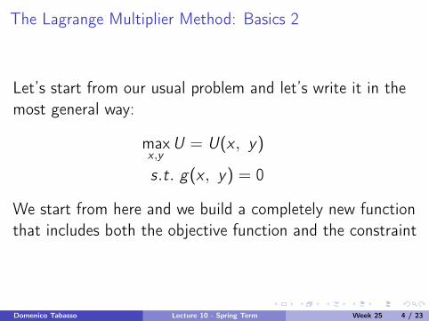
Let’s start from our usual problem and let’s write it in themost general way:
maxx ,y
U = U(x , y)
s.t. g(x , y) = 0
We start from here and we build a completely new functionthat includes both the objective function and the constraint
Domenico Tabasso (University of Essex - Department of Economics)Lecture 10 - Spring Term Week 25 4 / 23
The Lagrange Multiplier Method: Basics 3
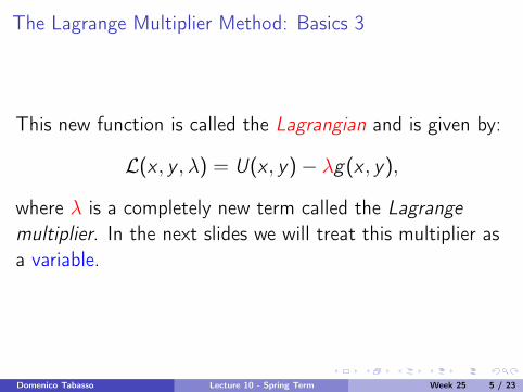
This new function is called the Lagrangian and is given by:
L(x , y , λ) = U(x , y)− λg(x , y),
where λ is a completely new term called the Lagrangemultiplier. In the next slides we will treat this multiplier asa variable.
Domenico Tabasso (University of Essex - Department of Economics)Lecture 10 - Spring Term Week 25 5 / 23
The Lagrange Multiplier Method: Basics 3
This new function is called the Lagrangian and is given by:
L(x , y , λ) = U(x , y)− λg(x , y),
where λ is a completely new term called the Lagrangemultiplier. In the next slides we will treat this multiplier asa variable.
Domenico Tabasso (University of Essex - Department of Economics)Lecture 10 - Spring Term Week 25 5 / 23
The Lagrange Multiplier Method: Basics 4
So our function L is a function of three variables: x , yand λ.
This implies that if we want to find a maximum, wehave to maximize with respect to all three variables.
Hence the first order conditions will be given by threeequations
Domenico Tabasso (University of Essex - Department of Economics)Lecture 10 - Spring Term Week 25 6 / 23

The Lagrange Multiplier Method: Maximizing the Lagrangian Function
First Order Conditions:
∂L(x , y , λ)
∂x= 0
∂L(x , y , λ)
∂y= 0
∂L(x , y , λ)
∂λ= 0
at x = x∗, y = y ∗ and λ = λ∗.
Domenico Tabasso (University of Essex - Department of Economics)Lecture 10 - Spring Term Week 25 7 / 23
The Lagrange Multiplier Method: Maximizing the Lagrangian Function
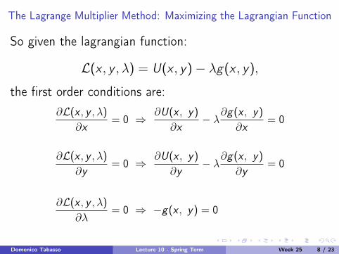
So given the lagrangian function:
L(x , y , λ) = U(x , y)− λg(x , y),
the first order conditions are:∂L(x , y , λ)
∂x= 0 ⇒ ∂U(x , y)
∂x− λ∂g(x , y)
∂x= 0
∂L(x , y , λ)
∂y= 0 ⇒ ∂U(x , y)
∂y− λ∂g(x , y)
∂y= 0
∂L(x , y , λ)
∂λ= 0 ⇒ −g(x , y) = 0
Domenico Tabasso (University of Essex - Department of Economics)Lecture 10 - Spring Term Week 25 8 / 23
The Lagrange Multiplier Method: Maximizing the Lagrangian Function
Note that the third first order condition is simply theconstraint itself, written in the implicit way.
In order to find our optimal x∗, y ∗ and λ∗ we have to solvethe previous system of three equations in three unknowns.
This goal can be achieved making use of the fact that allthe equations are equal to 0 and hence equal to each other.
Domenico Tabasso (University of Essex - Department of Economics)Lecture 10 - Spring Term Week 25 9 / 23
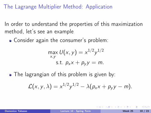
The Lagrange Multiplier Method: Application
In order to understand the properties of this maximizationmethod, let’s see an example
Consider again the consumer’s problem:
maxx ,y
U(x , y) = x1/2y 1/2
s.t. pxx + pyy = m.
The lagrangian of this problem is given by:
L(x , y , λ) = x1/2y 1/2 − λ(pxx + pyy −m).
Domenico Tabasso (University of Essex - Department of Economics)Lecture 10 - Spring Term Week 25 10 / 23
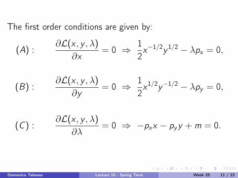
The first order conditions are given by:
(A) :∂L(x , y , λ)
∂x= 0 ⇒ 1
2x−1/2y 1/2 − λpx = 0,
(B) :∂L(x , y , λ)
∂y= 0 ⇒ 1
2x1/2y−1/2 − λpy = 0,
(C ) :∂L(x , y , λ)
∂λ= 0 ⇒ −pxx − pyy + m = 0.
Domenico Tabasso (University of Essex - Department of Economics)Lecture 10 - Spring Term Week 25 11 / 23
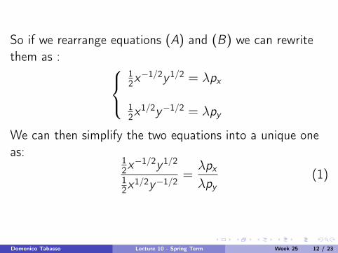
So if we rearrange equations (A) and (B) we can rewritethem as :
12x−1/2y 1/2 = λpx
12x
1/2y−1/2 = λpy
We can then simplify the two equations into a unique oneas:
12x−1/2y 1/2
12x
1/2y−1/2=λpx
λpy(1)
Domenico Tabasso (University of Essex - Department of Economics)Lecture 10 - Spring Term Week 25 12 / 23
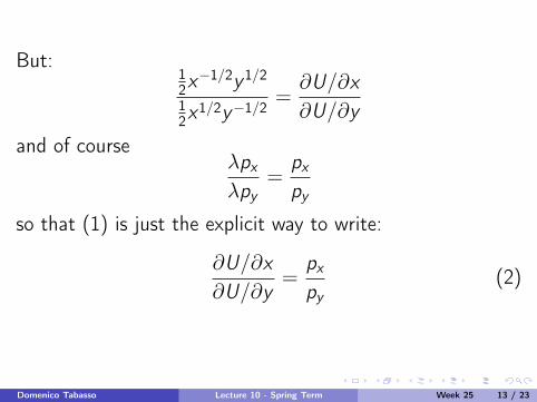
But:12x−1/2y 1/2
12x
1/2y−1/2=∂U/∂x∂U/∂y
and of courseλpx
λpy=
px
py
so that (1) is just the explicit way to write:
∂U/∂x∂U/∂y
=px
py(2)
Domenico Tabasso (University of Essex - Department of Economics)Lecture 10 - Spring Term Week 25 13 / 23
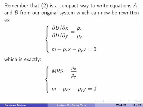
Remember that (2) is a compact way to write equations Aand B from our original system which can now be rewrittenas:
∂U/∂x∂U/∂y
=px
py
m − pxx − pyy = 0
which is exactly: MRS =
px
py
m − pxx − pyy = 0
Doesn’t it look familiar?!?!
Domenico Tabasso (University of Essex - Department of Economics)Lecture 10 - Spring Term Week 25 14 / 23
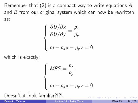
Remember that (2) is a compact way to write equations Aand B from our original system which can now be rewrittenas:
∂U/∂x∂U/∂y
=px
py
m − pxx − pyy = 0
which is exactly: MRS =
px
py
m − pxx − pyy = 0
Doesn’t it look familiar?!?!Domenico Tabasso (University of Essex - Department of Economics)Lecture 10 - Spring Term Week 25 14 / 23
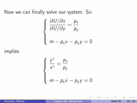
Now we can finally solve our system. So:∂U/∂x∂U/∂y
=px
py
m − pxx − pyy = 0
implies y ∗
x∗=
px
py
m − pxx − pyy = 0
Domenico Tabasso (University of Essex - Department of Economics)Lecture 10 - Spring Term Week 25 15 / 23

Solving in our usual way the first equation implies that:
y ∗
x∗=
px
py=⇒ pxx∗ = pyy ∗.
In addition, (C) implies that at the solution to the firstorder conditions:
pxx∗ + pyy ∗ = m.
Combined we find that:
pxx∗ = pyy ∗ =m2
=⇒ x∗ =m2px
, y ∗ =m2py
.
which are our standard results.
Domenico Tabasso (University of Essex - Department of Economics)Lecture 10 - Spring Term Week 25 16 / 23

How about λ?
So far we have found x∗ and y ∗. How about theoptimal value of our third variable, λ∗?
Well, once we have found x∗ and y ∗ finding λ∗ is trivial.
If we consider for example equation (A) of our initialsystem we have:
12x−1/2y 1/2 − λpx = 0
Domenico Tabasso (University of Essex - Department of Economics)Lecture 10 - Spring Term Week 25 17 / 23
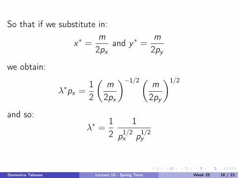
So that if we substitute in:
x∗ =m2px
and y ∗ =m2py
we obtain:
λ∗px =12
(m2px
)−1/2( m2py
)1/2
and so:λ∗ =
12
1
p1/2x p1/2
y
Domenico Tabasso (University of Essex - Department of Economics)Lecture 10 - Spring Term Week 25 18 / 23
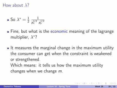
How about λ?
So λ∗ = 12
1p1/2x p1/2
y
Fine, but what is the economic meaning of the lagrangemultiplier, λ∗?
It measures the marginal change in the maximum utilitythe consumer can get when the constraint is weakenedor strengthened.Which means: it tells us how the maximum utilitychanges when we change m.
Domenico Tabasso (University of Essex - Department of Economics)Lecture 10 - Spring Term Week 25 19 / 23

Here, the maximum utility the consumer can get is:
U(x∗, y ∗) =
(m2px
)1/2( m2py
)1/2
=m
2p1/2x p1/2
y
= U(px , py ,m)
where U(px , py ,m) is the indirect utility function that westudied last week.
Domenico Tabasso (University of Essex - Department of Economics)Lecture 10 - Spring Term Week 25 20 / 23
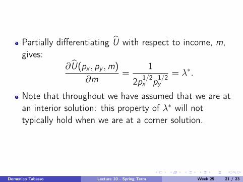
Partially differentiating U with respect to income, m,gives:
∂U(px , py ,m)
∂m=
1
2p1/2x p1/2
y= λ∗.
Note that throughout we have assumed that we are atan interior solution: this property of λ∗ will nottypically hold when we are at a corner solution.
Domenico Tabasso (University of Essex - Department of Economics)Lecture 10 - Spring Term Week 25 21 / 23
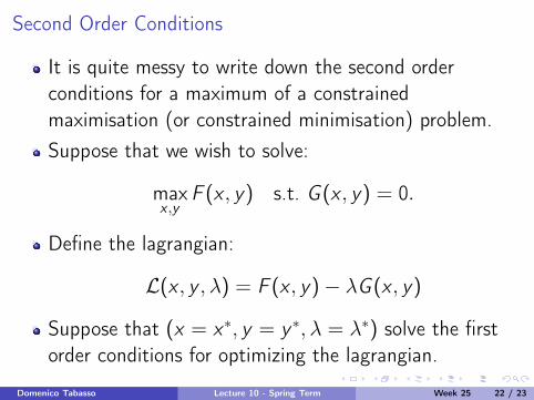
Second Order Conditions
It is quite messy to write down the second orderconditions for a maximum of a constrainedmaximisation (or constrained minimisation) problem.Suppose that we wish to solve:
maxx ,y
F (x , y) s.t. G (x , y) = 0.
Define the lagrangian:
L(x , y , λ) = F (x , y)− λG (x , y)
Suppose that (x = x∗, y = y ∗, λ = λ∗) solve the firstorder conditions for optimizing the lagrangian.
Domenico Tabasso (University of Essex - Department of Economics)Lecture 10 - Spring Term Week 25 22 / 23

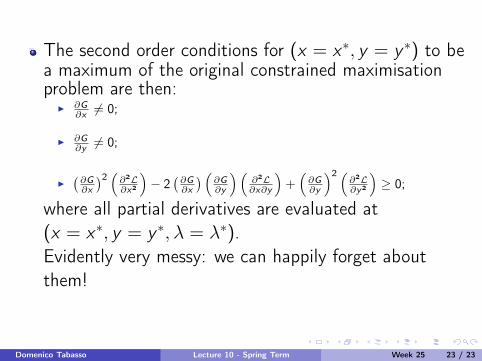
The second order conditions for (x = x∗, y = y ∗) to bea maximum of the original constrained maximisationproblem are then:
I ∂G∂x 6= 0;
I ∂G∂y 6= 0;
I(
∂G∂x
)2 (∂2L∂x2
)− 2
(∂G∂x
) (∂G∂y
)(∂2L∂x∂y
)+(
∂G∂y
)2 (∂2L∂y2
)≥ 0;
where all partial derivatives are evaluated at(x = x∗, y = y ∗, λ = λ∗).
Evidently very messy: we can happily forget aboutthem!
Domenico Tabasso (University of Essex - Department of Economics)Lecture 10 - Spring Term Week 25 23 / 23
The second order conditions for (x = x∗, y = y ∗) to bea maximum of the original constrained maximisationproblem are then:
I ∂G∂x 6= 0;
I ∂G∂y 6= 0;
I(
∂G∂x
)2 (∂2L∂x2
)− 2
(∂G∂x
) (∂G∂y
)(∂2L∂x∂y
)+(
∂G∂y
)2 (∂2L∂y2
)≥ 0;
where all partial derivatives are evaluated at(x = x∗, y = y ∗, λ = λ∗).Evidently very messy: we can happily forget aboutthem!
Domenico Tabasso (University of Essex - Department of Economics)Lecture 10 - Spring Term Week 25 23 / 23