Algorithmica (1989) 4:97-108 Algorithmica �9 1989 Springer-Verlag New York Inc.

Constrained Delaunay Triangulations 1

L. Paul Chew 2

Abstract. Given a set of n vertices in the plane together with a set of noncrossing, straight-line edges, the constrained Delaunay triangulation (CDT) is the triangulation of the vertices with the following properties: (1) the prespecified edges are included in the triangulation, and (2) it is as close as possible to the Delaunay triangulation. We show that the CDT can be built in optimal O(n log n) time using a divide-and-conquer technique. This matches the time required to build an arbitrary (unconstrained) Delaunay triangulation and the time required to build an arbitrary con- strained (non-Delaunay) triagulation. CDTs, because of their relationship with Delaunay triangula- tions, have a number of properties that make them useful for the finite-element method. Applications also include motion planning in the presence of polygonal obstacles and constrained Euclidean minimum spanning trees, spanning trees subject to the restriction that some edges are prespecified.

Key Words. Triangulation, Delaunay triangulation, Constrained triangulation, Algorithm, Voronoi diagram.

1. Introduction. Assume we are given an n-vertex, planar, straight-line graph G. A constrained triangulation of G is a t r iangulat ion o f the vertices o f G t h a t includes the edges o f G as par t o f the tr iangulation. See [PS85] for an explanat ion o f how such a t r iangulat ion can be found in O(nlogn) time. A constrained Delaunay triangulation (CDT) of G (called an obstacle tr iangulat ion in [Ch86] or a general ized De launay tr iangulat ion in [Le78] and [LL86]) is a constrained tr iangulat ion o f G that also has the proper ty that it is as close to a Delaunay triangulation as possible.

In this paper we show that, by using a method similar to that used by Y a p [Ya84] for building the Voronoi diagram o f a set o f simple curved segments, the C D T of G can be built in O(nlogn) time, the same time b o u n d required to build the (unconstrained) De launay triangulation. This also matches the time needed to build a constrained (non-Delaunay) tr iangulation. Earlier work has shown that the C D T can be built in O(n 2) time [DFP85] , [LL86]. An O( nlogn )-time algori thm for the special case when the edges o f G form a simple po lygon was presented in ILL86].

The Delaunay triangulation is the straight-line dual o f the Voronoi diagram (see Figure 1). See [PS85] for definitions and a number o f applicat ions o f De launay tr iangulations and Voronoi diagrams.

An impor tan t proper ty o f the Delaunay tr iangulat ion is that edges cor respond to empty circles. Indeed, this proper ty can be used as the definition o f De launay

An earlier version of the results presented here appeared in the Proceedings of the Third Annual Symposium on Computational Geometry (1987)v 2 Department of Mathematics and Computer Science, Dartmouth College, Hanover, NH 03755, USA.

Received May 23, 1987; revised November 27, 1987. Communicated by Chee-Keng Yap.

98 L.P. Chew

Q

Fig. 1. A Voronoi diagram and the corresponding Delaunay triangulation.

triangulation. It is straightforward to show that this definition is equivalent to the more common definition of the Delaunay triangulation as the dual of the Voronoi diagram.

DEFINITION. Let S be a set of points in the plane. A triangulation T is a Delaunay triangulation of S if for each edge e of T there exists a circle c with the following properties:

(1) The endpoints of edge e are on the boundary of c. (2) No other vertex of S is in the interior of c.

If no four points of S are cocircular then the Delaunay triangulation is unique. For most cases in which there is not a unique Delaunay triangulation, any of them will do.

The following definition, equivalent to the definition given in [LET8], indicates what we mean when we say "as close as possible to the Delaunay triangulation". Compare this definition with the definition of the (unconstrained) Delaunay triangulation given above.

DEFINITION. Let G be a straight-line planar graph. A triangulation T is a constrained Delaunay triangulation (CDT) of G if each edge of G is an edge of T and for each remaining edge e of T there exists a circle c with the following properties:

(1) The endpoints of edge e are on the boundary of c. (2) If any vertex v of G is in the interior of c then it cannot be "seen" from at

least one of the endpoints of e (i.e., if you draw the line segments from v to

Constrained Delaunay Triangulations 99

Fig. 2. A graph G and the corresponding constrained Delaunay triangulation

each endpoint of e then at least one of the line segments crosses an edge of G).

It follows immediately from the definition that if G has no edges then the constrained Delaunay triangulation is the same as the (unconstrained) Delaunay triangulation.

We distinguish two types of edges that appear in a CDT: G-edges, prespecified edges that are forced upon us as part of G, and Delaunay edges, the remaining edges of the CDT (see Figure 2).

Intuitively, the definitions of Delaunay triangulation and constrained Delaunay triangulation are the same except that, for the CDT, we ignore portions of a circle whenever the circle passes through an edge of G. Note that the CDT is not the same as the dual of the line-segment Voronoi diagram. The line-segment Voronoi diagram can have parabolas appearing as portions of Voronoi boun- daries. Its dual would include edges connecting obstacle edges, while the CDT has edges only between vertices. O(n log n)-time algorithms for constructing the line-segment Voronoi diagram appear in [Ki79] and [Ya84].

One measure of the appropriateness of a definition is its utility. We demonstrate the utility of the definition of a CDT by presenting some applications. Just as the (unconstrained) Delaunay triangulation of S can be used to determine the Euclidean minimum spanning tree (EMST) of S quickly, the CDT can be used to find the constrained EMST of S, constrained in the sense that certain edges of the spanning tree are prespecified and may not be crossed by other edges of the spanning tree. A simple proof by contradiction shows that the EMST is a subgraph of the Delaunay triangulation for both the constrained and uncon- strained versions. See [ PS85] for a version of the proof for the unconstrained case.

An additional application is presented in [Ch86] and [Ch87a] where variations of the standard CDT are used for motion planning in the plane. These variations use a different distance function, in effect using a "circle" that is shaped like a

100 L.P. Chew

square [Ch86] or a triangle [Ch87a]. With some modifications, the results presen- ted here are valid for CDTs based on the square-distance (the L1 metric) or the triangle-distance or based on other convex distance functions. (One such modification is that the word triangulation is inappropriate--some regions cannot be divided into triangles. In this case, the CDT can be defined as a planar graph with the empty circle property and with the maximum number of edges.) See [CD85] for more information on convex distance functions and their relation to Delaunay triangulations.

CDTs are also useful for the finite element method, a widely used technique for obtaining approximate numerical solutions to a wide variety of engineering problems. For many applications of this method, the first step is to triangulate a given region in the plane. Not just any triangulation will do; error bounds are best if all the triangles are as close as possible to equilateral triangles. Presently, either these triangulations are produced by hand or they are produced automati- cally using one of a number of heuristic techniques. In [Ch87b] we present an efficient new technique, based on CDTs, for producing desirable triangulations. Constrained Delaunay triangulations are necessary because some edges are pre- specified: boundary edges for the problem region plus optional user-chosen edges in the interior of the region. Unlike previous techniques, this technique comes with a guarantee: the angles in the resulting triangulations are all between 30 ~ and 120 ~ and the edge lengths are all between h/2 and h where h is a parameter chosen by the user.

Another application of CDTs has been suggested in [DFP85] and ILL86], where CDTs are used for surface interpolation~ For instance, in geographical surface interpolation, in addition to values at specific points, certain boundaries may be known (e,g., a lake boundary or a mountain ridge). A CDT provides a natural way to retain the boundary information while producing a good triangu- lation.

2. The Algorithm. We use divide-and-conquer to build the CDT. For simplicity of presentation, we assume that the planar graph G is contained within a given rectangle. We start by sorting the vertices of G by x-coordinate; then we use this information to divide the rectangle into vertical strips in such a way that there is exactly one vertex in each strip. Of course, this cannot be done if some vertex is directly above another, but we can avoid this problem by rotating the entire graph G if necessary. Following the divide-and-conquer paradigm, the CDT is calculated for each strip, adjacent strips are pasted together in pairs to form new strips, and the CDT is calculated for each such newly formed strip until the CDT for the entire G-containing rectangle has been built. This whole process takes time O(n log n) provided the CDT pasting operation can be done efficiently.

The trick used to ensure that this CDT pasting operation is done in reasonable time is to avoid keeping track of too much edge information. Note that it is not possible to keep track of all places where G-edges intersect strip boundaries; if we do so then we could have as many as O(n 2) intersections to work with. Edges that cross a strip, edges with no endpoints within the strip, are, for the most part,

Constrained Delaunay Triangulations 101

I P -

, - . . . .

ii Fig. 3. The contents of a strip and the contents that we keep track of.

ignored. Such an edge is of interest only if it interacts in some way with a vertex that lies within the strip. Yap [Ya84] used the same technique to develop an algorithm for the line-segment Voronoi diagram.

Each strip, then, is divided into regions by cross edges, G-edges that have no endpoint within the strip. We do not keep track of all of these regions (there could be O(n 2) of them). Instead we keep track of just the regions that contain one or more vertices (see Figure 3).

At this point, two parts of the CDT algorithm require further explanation: (1) how to handle vertex-containing regions, initializing them and keeping track of them as adjacent strips are combined, and (2) how to stitch together CDTs as adjacent strips are combined.

3. Control of Vertex-Containing Regions. Each initial strip has a single region containing its single vertex. To create these initial regions we need to know the edge immediately above and the edge immediately below each vertex. (Note that the edge immediately above a vertex may be the top edge of the rectangle that contains the entire graph G and the edge immediately below may be the bottom edge of the rectangle.) This information can be found for all vertices in O(n log n) time by using a vertical line as a sweep-line. See [PS85] for an explanation of this technique and a number of applications.

It is not difficult to determine appropriate regions when two adjacent strips are stitched together. Basically, we merge regions by running through the regions in their order along the strips (see Figure 4). As we move from bottom to top in the combined strip, we start a new region whenever either strip starts a region, we continue the region as long as a region continues in either strip, we stop a region only when we reach a point where neither strip has a vertex-containing

102 L.P. Chew

]o~

Fig. 4. Merging the regions of two adjacent strips.

region. A s w e do this merge process, we create an ordered list of the important G-edges that cross the boundary between the two strips. Recall that cross edges (G-edges with endpoints outside either strip) are ignored. It is easy to see that this merge operation can be done in time O(v+h) where v is the number o f G-vertices within the two strips and h is the number of half-edges within the two strips.

A half-edge is one half of a G-edge; it starts at a vertex which must be within the strip, but its other end may be anywhere. A standard G-edge is made of two half-edges.

4. Infinite Vertices. How can we efficiently combine the CDTs of adjacent strips? Each strip contains one or more vertex-containing regions; each such region contains a CDT. If we must search each CDT to combine it with a CDT from an adjacent strip, and if such a search takes more than constant time for each vertex-containing region, then we lose the O(n log n)-time bound for building the complete CDT. Thus, we need an efficient way to access the CDTs within a strip.

To do this, we link such CDTs by introducing false vertices. A false vertex is introduced wherever an edge crosses a strip boundary. Note that, as before, this is not done for all edges; instead, we use only those G-edges which either (1) form a region boundary for a vertex-containing region, or (2) have exactly one endpoint within the strip. The total number of false vertices is thus O(v+h), where v is the number of G-vertices within the strip and h is the number of half-edges within the strip.

CDTs of adjacent regions are combined by executing the following steps: (1) eliminate false vertices (and Delaunay-edges that use these vertices) along the

Constrained Delaunay Triangulations 103

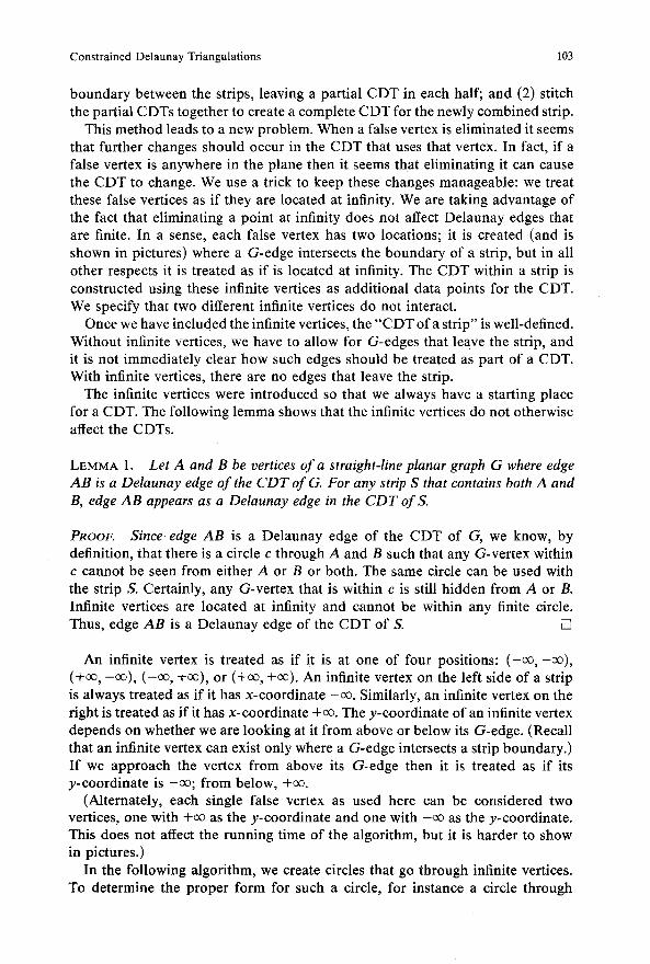
boundary between the strips, leaving a partial CDT in each half; and (2) stitch the partial CDTs together to create a complete CDT for the newly combined strip.

This method leads to a new problem. When a false vertex is eliminated it seems that further changes should occur in the CDT that uses that vertex. In fact, if a false vertex is anywhere in the plane then it seems that eliminating it can cause the CDT to change. We use a trick to keep these changes manageable: we treat these false vertices as if they are located at infinity. We are taking advantage of the fact that eliminating a point at infinity does not affect Delaunay edges that are finite. In a sense, each false vertex has two locations; it is created (and is shown in pictures) where a G-edge intersects the boundary of a strip, but in all other respects it is treated as if is located at infinity. The CDT within a strip is constructed using these infinite vertices as additional data points for the CDT. We specify that two different infinite vertices do not interact.

Once we have included the infinite vertices, the " C D T of a strip" is well-defined. Without infinite vertices, we have to allow for G-edges that leave the strip, and it is not immediately clear how such edges should be treated as part of a CDT. With infinite vertices, there are no edges that leave the strip.

The infinite vertices were introduced so that we always have a starting place for a CDT. The following lemma shows that the infinite vertices do not otherwise affect the CDTs.

LEMMA 1. Let A and B be vertices of a straight-line planar graph G where edge AB is a Delaunay edge of the CDT of G. For any strip S that contains both A and B, edge AB appears as a Delaunay edge in the CDT of S.

PROOF. Since edge AB is a Delaunay edge of the CDT of G, we know, by definition, that there is a circle c through A and B such that any G-vertex within c cannot be seen from either A or B or both. The same circle can be used with the strip S. Certainly, any G-vertex that is within c is still hidden from A or B. Infinite vertices are located at infinity and cannot be within any finite circle. Thus, edge AB is a Delaunay edge of the CDT of S. []

An infinite vertex is treated as if it is at one of four positions: ( - o % - c o ) , (+o% - ~ ) , (-oo, +o@, or (+oo, +co). An infinite vertex on the left side of a strip is always treated as if it has x-coordinate -oo. Similarly, an infinite vertex on the right is treated as if it has x-coordinate +c~. The y-coordinate of an infinite vertex depends on whether we are looking at it f rom above or below its G-edge. (Recall that an infinite vertex can exist only where a G-edge intersects a strip boundary.) I f we approach the vertex from above its G-edge then it is treated as if its y-coordinate is -oo; f rom below, +oo.

(Alternately, each single false vertex as used here can be considered two vertices, one with +oo as the y-coordinate and one with - ~ as the y-coordinate. This does not affect the running time of the algorithm, but it is harder to show in pictures.)

In the following algorithm, we create circles that go through infinite vertices. To determine the proper form for such a circle, for instance a circle through

104 L.P. Chew

(cO, o0), the reader should first consider a circle using the point (w, w), where w is a large number. Use the limit circle as w approaches oo. The limit circle will be a half-plane.

5. Combining CDTs of Adjacent Strips. The method we use for combining CDTs is similar to one of the methods used by Lee and Schachter [LS80] to build (unconstrained) Delaunay triangulations. This method is roughly equivalent to the process of constructing the dividing chain in the divide-and-conquer algorithm for building the standard Voronoi diagram. See [PS85] for an explanation of the Voronoi-diagram algorithm.

We assume the following operations can be done in unit time: (1) given point P and circle c, test whether P is in the interior of c; (2) given points P, Q, and R, return the circle through these points. These functions clearly take constant time for any reasonable model of computation, even if we use nonstandard "circles" as in [CD85].

Let A and B be vertices of G. Assume edge AB crosses the boundary between the two strips and that edge AB is known to be part of the desired CDT (AB may be either a G-edge or a just-created Delaunay edge). Consider a circle with points A and B on its boundary and with center well below edge AB. Change the circle by moving the center upward toward AB always keeping A and B on the boundary. Continue moving the center upward until the circle intersects the first vertex above edge AB that can be seen from both A and B. Call this vertex X (see Figure 5). It is easy to see that, by definition, the edges A X and BX are Delaunay edges of the CDT.

This process, as outlined in the previous paragraph, gives a nice intuitive way to find X, but we need an efficient algorithm for determining this vertex. Vertex X is either in B's strip or in A's strip; we assume for the moment that X is in A's strip. By Lemma 1, we know A X exists in the CDT of the left-hand strip. We conclude from this that for edge AB, the next boundary-crossing Delaunay-

t

i

I

x

A B

I i * l i

Fig. 5. Vertex X is the first vertex that can be seen from A and B.

Constrained Delaunay Triangulations 105

edge above AB must go from B to some vertex Y already connected to A, or from A to some vertex Z already connected to B. Of course, we cannot tell ahead of time whether the vertex we are looking for is on the left or the right, so we choose the best candidate vertex on each side, then we choose between them.

We still need to develop an efficient way to determine which of the vertices connected to A is the best candidate. We know from the argument above that for X (the vertex we are looking for) edge AX has to be a Delaunay edge; further, circle ABX is an empty circle for edge AX. In other words, a vertex Y, adjacent to A, can be eliminated as a possible candidate if circle A B Y contains a vertex that can be seen from A and Y.

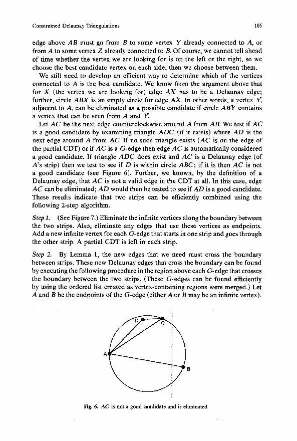
Let AC be the next edge counterclockwise around A from AB. We test if AC is a good candidate by examining triangle ADC (if it exists) where AD is the next edge around A from AC. If no such triangle exists (AC is on the edge of the partial CDT) or if AC is a G-edge then edge AC is automatically considered a good candidate. If triangle ADC does exist and AC is a Delaunay edge (of A's strip) then we test to see if D is within circle ABC; if it is then AC is not a good candidate (see Figure 6). Further, we known, by the definition of a Delaunay edge, that AC is not a valid edge in the CDT at all. In this case, edge AC can be eliminated; AD would then be tested to see if AD is a good candidate. These results indicate that two strips can be efficiently combined using the following 2-step algorithm.

Step 1. (See Figure 7.) Eliminate the infinite vertices along the boundary between the two strips. Also, eliminate any edges that use these vertices as endpoints. Add a new infinite vertex for each G-edge that starts in one strip and goes through the other strip. A partial CDT is left in each strip.

Step 2. By Lemma 1, the new edges that we need must cross the boundary between strips. These new Delaunay edges that cross the boundary can be found by executing the following procedure in the region above each G-edge that crosses the boundary between the two strips. (These G-edges can be found efficiently by using the ordered list created as vertex-containing regions were merged.) Let A and B be the endpoints of the G-edge (either A or B may be an infinite vertex).

A B

i g

Fig. 6. A C is not a good candidate and is eliminated.

106 L .P . Chew

i

Fig. 7. Step 1: eliminating infinite vertices as strips are combined. Open circles represent infinite vertices.

loop Eliminate A-edges that can be shown to be illegal because of their

interaction with B; Eliminate B-edges that can be shown to be illegal because of their

interaction with A; Let C be a candidate where AC is the next edge counterclockwise

around A from AB (if such an edge exists); Let D be a candidate where BD is the next edge clockwise around B

from BA (if such an edge exists); exit loop if no candidates exist; Let X be the candidate that corresponds to the lower of circles ABC

and ABD; Add edge AX or BX as appropriate and call this new edge AB; end loop;

Using the process outlined above, the time to combine the CDTs of adjacent strips is O(v + h) where v is the total number of vertices in the newly combined strip and h is the number of half-edges from each of the two strips. To see this note that in each part of step 2 we either eliminate an edge from a partial CDT or we add an edge for the combined CDT. It is easy to see that the total number of edges involved is O(v + h).

We claim that the time to build the complete CDT for a straight-line planar graph G is O(n log n) where n is the number of vertices of G. The problem is initially broken down into n strips each containing a single vertex. Strips are combined in pairs to make strips containing two vertices, then four vertices, etc. These subproblems can be represented in a tree of depth O(log n) with the complete CDT at the root and with single-vertex strips appearing as the leaves. Recall that the time to solve one subproblem is O(v + h) where v is the number of vertices within the strip and h is the number of half-edges for that strip. For

Constrained Delaunay Triangulations 107

a single level of the tree, each vertex of G appears in exactly one subproblem and each half-edge of G (a G-edge is always made of two half-edges) appears in exactly one subproblem. Thus, the total time spent solving all the subproblems on one level of the tree is O(n + e) where e is the number of edges in G. Since G is planar, e is O(n). This give us the following theorem.

THEOREM. Let G be a straight-line planar graph. The CDT of G can be built in O(n log n) time where n is the number of vertices of G.

6. Conclusions. We have shown how a divide-and-conquer algorithm can be used to produce the CDT in O(n log n) time. This time bound is optimal since it is easy to show that a CDT can be used to sort. There are two ideas that have been particularly important in reaching this time bound: (1) as in [Ya84], the only cross edges that we keep track of are those that bound vertex-containing regions; (2) infinite vertices are used so that partial CDTs are linked for efficient access. A useful property of these infinite vertices is that such a vertex can be eliminated with minimal effect on edges between noninfinite vertices.

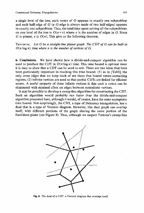
It may be possible to develop a sweep-line algorithm for constructing the CDT. Such an algorithm would probably run faster than the divide-and-conquer algorithm presented here, although it would, of course, have the same asymptotic time bound. Not surprisingly, the CDT, a type of Delaunay triangulation, has a dual that is a type of Voronoi diagram. However, this dual graph can overlap itself, with different portions of the graph sharing the same portion of the Euclidean plane (see Figure 8). Thus, although we suspect Fortune's sweep-line

Fig. 8. The dual of a CDT: a Voronoi diagram that overlaps itself.

108 L.P. Chew

technique [Fo87], developed to build the standard Voronoi diagram, can be adapted to build the CDT, it is not immediately clear how it should be done.

References

[CD85]

[Ch86]

[Ch87a]

[Ch87b] [DFP85]

[Fo87] [Ki79]

[Le78]

[LL86]

[LS80]

[PS85]

[Ya84]

L. P. Chew and R. L. Drysdale, Voronoi diagrams based on convex distance functions, Proceedings of the First Symposium on Computational Geometry, Baltimore (1985), pp. 235-244. (Revised version submitted to Discrete and Computational Geometry.) L. P. Chew, There is a planar graph almost as good as the complete graph, Proceedings of the Second Annual Symposium on Computational Geometry, Yorktown Heights (1986), pp. 169-177. L. P. Chew, Planar graphs and sparse graphs for efficient motion planning in the plane, in preparation. L. P. Chew, Guaranteed-quality triangular meshes, in preparation. L. De Flofiani, B. Falcidieno, and C. Pienovi, Delaunay-based representation of surfaces defined over arbitrarily shaped domains, Computer Vision, Graphics, and Image Processing, 32 (1985), 127-140. S. Fortune, A Sweepline algorithm for Voronoi diagrams, Algorithmica, 2 (1987), 153-174. D. G. Kirkpatrick, Efficient computation of continuous skeletons, Proceedings of the 20th Annual Symposium on the Foundations of Computer Science, IEEE Computer Society (1979), pp. 18-27. D. T. Lee, Proximity and teachability in the plane, Technical Report R-831, Coordinated Science Laboratory, University of Illinois (1978). D. T. Lee and A. K. Lin, Generalized Delaunay triangulation for planar graphs, Discrete and Computational Geometry, 1 (1986), 201-217. D. T. Lee and B. Schachter, Two algorithms for constructing Delaunay triangulations, International Journal of Computer and Information Sciences, 9 (1980), 219-242. F. P. Preparata and M. I. Shamos, Computational Geometry, Springer-Verlag, New York (1985). C. K. Yap, An O(n log n)algorithm for the Voronoi diagram of a set of simple curve segments. Technical Report, Courant Institute, New York University (October 1984).