Constitutive equations in suspension mechanics. Part 2. Approximate forms for a suspension of

http://journals.cambridge.org Downloaded: 31 Jul 2009 IP address: 131.111.16.227

J . Fluid Mech. (1976), vol. 76, part 1, p p . 187-208 Printed in Great Britain

187

Constitutive equations in suspension mechanics. Part 2. Approximate forms for a suspension of rigid particles

affected by Brownian rotations By E. J. HINCH

Department of Applied Mathematics and Theoretical Physics, University of Cambridge

A N D L. G. LEAL Chemical Engineering, California Institute of Technology, Pasadena

(Received 3 July 1975)

Approximate constitutive equations are derived for a dilute suspension of rigid spheroidal particles with Brownian rotations, and the behaviour of the approximations is explored in various flows. Following the suggestion made in the general formulation in part 1, the approximations take the form of Hand’s (1962) fluid model, in which the anisotropic microstructure is described by a single second- order tensor. Limiting forms of the exact constitutive equations are derived for weak flows and for a class of strong flows. In both limits the microstructure is shown to be entirely described by a second-order tensor. The proposed approximations are simple interpolations between the limiting forms of the exact equations. Predictions from the exact and approximate constitutive equations are compared for a variety of flows, including some which are not in the class of strong flows analysed.

1. Introduction An urgent problem in rheology is the production of simple constitutive equa-

tions which provide a tolerable approximation to the behaviour of non-Newtonian fluids for a wide class of flows. I n part 1 of the present series (Hinch & Leal 1975, hereafter denoted as I), the basic formulation of suspension mechanics was analysed and a common simplified constitutive model was derived for materials which can be modelled as a suspension of particles (or macromolecules) in a Newtonian fluid. For small departures from equilibrium, it was shown that the microstructural features which determine the bulk stress for such materials can be completely described by a single second-order tensor. Thus, as shown earlier by BarthBs-Biesel & Acrivos (1973) for some specific suspensions, the constitutive model in this weak-flow limit reduces to a form of the second-order-tensor structural model of Hand (1962). In addition the limited information available led us to the suggestion (see I) that the microstructure in the strong-flow regime far from equilibrium can be characterized for many types of flow by a single direction and a single scalar parameter. The constitutive model in this limit thus

http://journals.cambridge.org


188 E . J . Hinch and L. G . Leal

reduces again to a simple form of Hand’s model. At intermediate flow strengths, however, the analysis of I demonstrates that something more general than a second-order tensor is needed for the rigorous description of the microstructure of the majority of suspension-like materials. The full constitutive model of I is thus more complex than either of its separate limits and further restrictions on its general form must be found which are not limited to very weak or very strong flows if it is to be of any practical value. We suggested in I that a form of Hand’s model which exactly represents the two limiting cases and interpolates smoothly between them may give a crude but simple first approximation of the exact constitutive behaviour of suspension-like materials which is useful over the whole range of flow strengths.

I n the present part of our study we investigate the potential of this suggestion for the special case of a dilute suspension of rigid spheroidal particles in the presence of Brownian rotation. The advantage of this material for our present purposes is the fact that exact constitutive equations are available, and have been evaluated in many particular flows (see the review by Leal & Hinch 1973). We begin by restating in $ 2 the exact constitutive equations, and their limiting forms for small and large departures from the equilibrium state of random orientation. Next, in 9 3 a simple composite approximation of the Hand type is derived which reproduces the limiting results exactly and interpolates smoothly between them. Finally, in $ 4 the accuracy of the simple approximate form is determined by comparison with results from the exact model for several different flow types.

2. The suspension 2.1. The exact constitutive equations

We consider a dilute suspension of rigid, axially symmetric particles which are free of external body forces or couples and are sufficiently small that the micro- dynamics are inertialess. When placed in a homogeneous time-dependent linear flow U(X, t ) = r ( t ) . X,

with r = ~ + n , E T = E , n ~ = - n , an isolated particle aligned in the direction of the unit vector p ( t ) rotates in t.he absence of Brownian couples according to

where G is a shape factor of modulus less than unity (except for very curious particles; Bretherton 1962). When Brownian couples act, the orientation of a single particle is given statistically by a probability density function N ( p , t ) which satisfies a Fokker-Planck equation in p space:

( 2 ) aNpt + v . [ ~ i , - DVNI = 0,

with 0 = p ( p ) given by (1) and D the rotational diffusivity. Equations (1) and ( 2 ) govern the evolution of the microstructure of the suspension, and correspond for



Constitutive equations in suspension mechanics. Part 2 189

this particular material to equations ( 3 b ) and (7) in the general formulation of I. The exact constitutive equations are completed by relating the bulk stress to the microstructural state as described by N . This is achieved using a volume average ofthe stress at the microscale of the suspended particles and results in

u = -pl + 2pE + 2p<Dt{2A (PPPP):E + 2BKPP) * E + E * (PP)l+ CE + F(PP)D}, (3)

where ,u is the Newtonian solvent viscosity, (D the small volume fraction of the particles and A , B, C and F four more shape factors. The angle brackets denote quantities which are averaged with respect to the probability density function N(p, t). Equation (3) corresponds for this particular material to equations (4) and (8) in the general formulation of I. A complete description of the derivation of the constitutive equations (1)-(3) can be found in Leal & Hinch (1973).

As we have noted in the introduction and in I, the majority of suspension-like materials require a more general description of the microstructure than can be provided by a single second-order tensor. The model suspension represented by (1)-(3) is no exception, since no explicit or implicit combination of the basic equations can be used to eliminate the fourth-order vector product (pppp). Prager (1957) has shown that a direct dynamic equation for (pp) can be obtained by multiplying (2) by pp - 91 and integrating over p space. The result is

D(PP)/Dt- Q * (PP) - (PP) * QT

- GEE. (PP) + (PP). ET- 2(PPPP):El +GDC(PP) - *I1 = 0. (4)

However, this equation for the development of (pp) contains the unknown higher moment (pppp). Similarly, an equation may be obtained for the development of any finite moment of p, but each such equation always involves a higher moment of p. There is thus no finite closed system of equations which is equivalent to (1)-(3) but simpler in f0rm.t To evaluate the rheological response of the model suspension for a general form r(t) and arbitrary flow strengths, one must first solve (2) for N(p, t), and substitute the result into (3). As indicated in I, only the limiting cases of very weak or very strong flow, corresponding to near-equilibrium or strongly non-equilibrium microstructure, are amenable to rigorous asymptotic solution.

2.2. Near-equilibrium approximations Lowest approximation. When the flow is very weak, the Brownian motions

produce an almost uniform orientation distribution :

N = (4n)-l +smaller terms.

The lowest approximations for the angle averages are therefore simply

(pp) = QI + ..., (PPPP):E = &E + ... . (5% b)

t It may be noted, however, that for steady bulk flow (4) does provide a definite algebraic relationship between (pppp): E and (pp), which may be used to express the bulk stress Q [equation (3)] entirely in terms of the second moment (pp).



190 E . J . Hinch and L. G. Leal

At this level of approximation, the relationship (3) between the bulk stress and bulk rate of strain is Newtonian in form, with an effective viscosity

p* = p [ l + ( & A + + B + C ) @ ] .

We now proceed to the next approximation. First correction. Neither the spin of the particle with the local vorticity nor the

rotational diffusion process disturbs the uniform orientation distribution. It is only the pure-strain component of the bulk motion which initially creates any preferred alignment of the particles. When the left-hand side of ( 2 ) is evaluated with the constant N , an unbalanced strain-induced term - (3/47r)G(p. E . p) remains. This forces a correction to N which is described by a second-order tensor anisotropy : N = (47r)-l(l+ +$p . A. p +smaller terms),

in which A(t) is small, O(E/D) , and both symmetric and traceless. The vorticity spin term in ( 2 ) rotates A, while the diffusion term decreases A’s magnitude. Both terms just alter the second-order tensor without producing any further type of anisotropy. The action of the straining motion on A does generate a new type of term but it is neglected a t the present level in the near-equilibrium approximation.

The development of A can be found directly from (2), and is governed a t this

( 6 ) level of approximation by

where 9/9t is the Jauman derivative

(9/9t+ 6D)A = +GE,

9Al9t = DA/Dt - 51. A - A. aT. Knowing A, we can obtain a better approximation than (5) to the important moments

(pp) = &I+A +..., (7a)

( 7 b ) (pppp): E = -&E++(A. E + E . A) ++IA: E + ... . At the next level of approximation, the bulk straining motion acting on A

generates a fourth-order tensor contribution to the orientation distribution function. As we have noted in the introduction, the present study is intended to investigate the potential of a second-order-tensor model for the approximate description of suspensions. Thus for our present purposes there is no need to proceed fully to this next level of approximation. The use of ( 7 ) in the A and B terms of the stress equation (3) is sufficient for the description of the first departures of these terms from the Newtonian (equilibrium structure) form. Equations ( 6 ) and (7) , however, produce only the Newtonian form for the F term in (3), DA = &GE, and it is thus necessary to proceed partially to the next level of approximation in order that the first departure of the bulk stress from the Newtonian form is fully described. Fortunately the difficult term involves only (PP), for which there is the exact equation (4). To obtain an adequate approximation to (4) for our purposes, we may use ( 7 ) in (4) and now define A exactly by (7a). Thus we replace ( 6 ) by

( 8 ) (9/9t + 6D)A = G[zE + + ( E . A+ A. E ) -+lA: E l .




In slowly varying weak flows in which \19/9tI\, llGEll < D equation (8) may be solved iteratively to obtain an explicit expression for A:

(E . E - 81 E : E) + . . . . 1 Substituting this into (3) gives the second-order-fluid approximation

2 2 GF 1 9 E 15 3 ") 15 90 D 9 t Q = - ~ I + ~ , u E + ~ , u @ - A + - B + C + - E- ---

- ( E.E-QIE:E)+ ...

Of course (7) and consequently (8) remain valid outside the slowly varying restriction of the second-order-fluid model. In more general situations A [as the solution of (S)] need only remain small in order to be consistent with the near- equilibrium approximation.

In later sect iclns of this paper, we shall use A to denote the non-isotropic part of (pp), as indicated in (7a). To obtain the correct Newtonian results for an equilibrium microstructure, ( 5 ) must be used in (3) and (4). The correct fist deviations from the Newtonian (equilibrium) form are obtained by using (7) in (3) and (4).

2.3. Approximate forms for the strong-$ow regime Lowed approximation. A prerequisite for obtaining an asymptotic representa-

tion of (1)-(3) in the limit of weak Brownian motion (strong flow) is an understanding of the particle behaviour when no random couples are present, i.e. the solutions of the initial-value problem represented by (1). Bretherton (1962) has shown how this nonlinear problem may be replaced by the linear one obtained by dropping the final term of (1). Thesolutionsto theoriginal equationremain parallel for all time to the solutions of the modified, linear equation. We consider here the subclass of possible flows in which the particles tend to align in a single direction independent of their initial orientation. Bretherton (1962) has shown that this subclass consists of those flows for which the real part of one of the eigenvalues of G? + GE exceeds the real parts of the other two eigenva1ues.t This condition is actually satisfied for G =l= 0 in all but a very small class of exceptional flows. Unfortunately many of the most common rheological flows fall into this exceptional class, including shear flows of all types, and certain axisymmetric straining motions. 1 Although simple shearing flows are thus strictly excluded from the present analysis, an earlier paper (Hinch & Leal 1972) shows that even these flows exhibit a sharply peaked orientation distribution for particles which have

t The initial orientations from which the particles do not align for a flow in this class are a set of measure zero and so would not contribute to the angle averages in (3). Further- more, in a real suspension, any weak Brownian couples which existed would move the particles out of these special orientations.

$ The specific axisymmetric straining flows which are to be considered as exceptional depend upon the sign of G (i.e. on the particle geometry). Foi G > 0 biaxial extensional flows are exceptions, while for G < 0 it is the uniaxial extensional flows which are excluded from the present theoretical development.




extreme axis ratios (i.e. G near k I), and it might be anticipated that such cases would not be badly approximated in the limit of weak Brownian motion by a theory which presumed total alignment in a single direction. We shall see, however, that shear flows for any G not near k 1 produce a distribution which is not sueciently localized for rigorous description by the asymptotic form for weak Brownian motion which we derive here. The error committed in the exceptional flows will provide one test of the tolerability of the approximate models.

Since we restrict attention to situations in which all particles tend to align in a single direction in the absence of Brownian rotation, the spread about that direction is expected to be small in the limit of weak Brownian motion. At the lowest approximation we therefore evaluate the moments (pp) and (pppp) as if all of the particles were aligned in the direction of a unit vector d :

1 (9) (pp) = dd +smaller terms,

(pppp): E = d d d d : E +smaller terms.

The equation governing the evolution of d may be seen from (1) to be

9 d / B t = G[ E . d - d d d : El. (10)

There are infinitely many ways of expressing the fourth moment in terms of the quadratic moment which are equivalent at this approximation, e.g.

(PPPP): E = (PP>(PP>: E + *.-

= (PP). E. (PP>+ ... = (PP)2 (PP>2: E/(I : (PP)2) + . * * * (11)

The choice between the alternative expressions depends on their behaviour outside this approximation.

Although attractive because of its simplicity, one serious drawback of the asymptotic approximation (9) and (10) is that it contains no internal check of consistency. If the particles are initially strongly aligned, then solving (10) forwards in time gives only the rate of change of the alignment direction, and provides no indication of whether the particles remain strongly aligned. An analogous situation does not occur in the near-equilibrium approximations since (6) and (8) can both show A increasing in magnitude as the near-equilibrium assumptions break down. To overcome this deficiency, we must proceed to the next level of approximation for the strong-flow asymptotic limit.

First correction. At this level, we must model the small spread in particle orientation which arises owing to the diffusive effect of weak Brownian rotation. The spread is concentrated near d by the variation of p(p) in the vicinity of d . Since the spread is small, the advection field (1) may be approximated to first order by its linear variation around p = d . Diffusion acting against a time- dependent linear advection produces a multivariate Gaussian distribution in N localized near d . The Gaussian is specified by its variance about d , and the evolution equation for the variance tensor can be calculated directly from (2).

We start by linearizing (1) about the direction d by putting p = d + 6 , with 6



Constitutive equations in swpension mechanics. Part 2 193

small and therefore approximately orthogonal to d. Substituting this expression into (1) and linearizing after separating out (10) yields

6 = Q.S+G[E.S-S(d.E.d)-2d(d.E.S)].

Part of the change in S is due to the rotation of d. This part is eliminated by projecting the last equation into the space orthogonal to the instantaneous d. Using the subscript 2 to denote variables associated with this two-dimensional subspace, we obtain S, = K2. 6,,

with the tensor K, defined as

K, = Q - dd. Q - Q. dd + G[E - dd. E - E . dd + 2dddd: E - dd: El].

The diffusion equation for the spread about d is then

aN 8 a2N - + - .(K,.S,N) = D- at as, as; 3

with the multivariate Gaussian solution N = (2n)-l (det B,)*exp ( - is,. B;l. 8,).

The variance tensor is denoted by B,, i.e. (S,S2) = B,, and its evolution is

B, = K,. B,+ B2. KT +2D1,. governed by

Finally we embed this two-dimensional tensor back into the original three- dimensional problem to form B. The last equation gives the development of those components of B in the space orthogonal to d. The remaining components can be calculated from the requirement that

B.d = 0 = d.B

must remain true in time as d rotates. Thus

B = (B,),-dd.B-B.dd+dd(d.B.d).

The equation governing the development of the full tensor B is then found to be

.9B/.9t = G[E.B+B.E-2B(dd:E)1+2D(I-dd). (12)

This equation is, of course, an approximation owing to the linearization of the advection equation (1) about d. If the spread of orientations is truly small, then B should be small, and the error in (12) is O(EGB2, DB). Indeed as (10) and (12) are integrated forwards in time, the relative magnitude of B provides the internal consistency check on the strong-flow assumption which was missing at the level of approximation represented by (9) and (10).

The preceding lowest-order analysis of the spread about d shows that the mean displacement of p from d is zero at O(S), that the variance is B at O(S2) and that higher moments are o(S2). In working accurately at O(S2), it is clear that a, better approximation is required for the localized mean value of p. There are two independent contributions to the mean displacement of p from d at O(S2). In order that p remains a unit vector, the O(S) displacements orthogonal to d

I 3 PLM 76



194 E. J. Hinch and L. G. Leal

must lead to an O(S2) shortening in the direction of d. This mean displacement is - $d(Sa = - *dl : B. I n the two-dimensional plane orthogonal to d, the mean displacement at 0 ( S 2 ) comes from the quadratic correction to the linear advection field described by

S, = K,. 6,- 2G[(I - dd)d. E. ( I - dd)]: S,S, + 0(S3). With this advection field, the solution of the diffusion equation is no longer a multivariate Gaussian distribution. To find the small correction to the mean displacement, the method of moments is adequate. If the advection-diffusion equation is multiplied by 6, and integrated over all 6, space (assuming that all terms decay to zero sufficiently rapidly as 6,+ a), the result is

(6,) = K,.(S,)-2G[(l-dd)d.E.(I-dd)]:(S,S,)+O(S3). Diffusion does not affect this first moment. I n the last term a sufficiently accurate estimate for (S,S,) is B,. Finally (S,), in the two-dimensional space, must be embedded back into the original three-dimensional space as(S), whichis to remain orthogonal to the moving d. Thus

= G[E. (S)- 2d(d. E . (6)) - (S)dd: E - 2B. E. d].

When proceeding to higher-order corrections beyond O(S2), the curvature of the unit sphere on which p lies must be considered.

The two O(8,) effects in the localized mean displacement of p from d can be combined with d to form the localized mean director a t O ( P ) :

d’= d(l-$l:B)+(S).

This modified director is not of unit length like the original d. The evolution equation for the modified director can be derived from the preceding analysis of its component parts:

(13) 9d’/Bt = G[E .d’- d’d’d’: E-d’E: B- 2B. E. d’] + 2Dd’,

neglecting small terms 0(S2E, D ) . The modified director d’ is the average of p using that part of the distribution

N localized around d. It is necessary to distinguish between such a localized average and the full average of p, which vanishes identically because of a symmetric part of N around - d. Viewing d’ as some sort of average of p is however very useful in providing an alternative derivation of (13) which bypasses all the detailed analysis of the contributing effects. The full distribution N must first be split into two parts N* which are defined everywhere but which are localized around kd, respectively. The task of separating N into its localized parts is intuitively simple only in the strong-flow limit. [One possible definition which can be applied mechanically to all flows is as follows. Take the unit vector d to be the largest principal axis of (pp) and define N* = $( 1 & (d. p)zn+l)N(p) with n a suitably large number.] The first moment of the full diffusion equation (2) using N + instead of N is

g(p)+/Bt = G[E. (P)+- (PPP)+: E] + ~D(P)+.




The equation for the modified director is recovered by identifying (p)+ with d’ and making a strong-flow approximation:

(ppp)+ = (p)+(p)+(p)+ + [(p)+B +permutations of indices] + o(cY2).

The trouble with this more direct approach is that any instantaneous definition of Nf must necessarily yield localized distribution functions which do not evolve according to the global diffusion equation (2). The simple intuitive interpretation of the strong-flow limit is, however, quite clear despite these mathematical difficulties.

The second approximation to the moments (9) can now be stated. They are simplest when expressed in terms of the localized mean and variance of p:

(pp) = d’d’ + B +0(S2) , (14a)

+ 2(d’d’. E . B + B . E . d’d’) + o(cY2). (1 4b)

These results are not dependent in any essential way on the detailed nature of the spread in the distribution about d. Indeed, any distribution which has N = O ( S F ~ ) as 8, becomes large, so that fourth moments are locally determined, would exhibit the same basic relationships when expressed in terms of the mean and variance of p. The exponential decay of a Gaussian amply satisfies this algebraic decay condition. The condition is not, however, generally satisfied in other cases, such as slender rod-like particles in simple shear flow, which appear to be strongly aligned in an averaged sense but are not members of the class of flows which produces alignment in a single direction.

Of the infinite number of ways of eliminating d’d’ and B between (14a) and (14b) with an accuracy O ( P ) , one of the simpler forms is

(pppp): E = d’d’d’d’: E + Bd’d’: E + d’d’B: E

(PPPP): E = (PP>(PP>: E +2[(PP>. E (PP>- (PP)2(PP)2: E/I:(PP)21, (15) with an error o(S2). By proceeding to this next approximation, one particular combination of the alternatives (1 1) has been selected. The simple form (15) has the desirable property of having the correct trace, (pp): E, a t all values of (pp).

The two evolution equations (10) and (12) can be combined using (14a) to give

q P P ) / a t = Q[E. (PP) + (PP). E - 2(PP)(PP): El +6D(Ql- (pp) )+O(GEB2,DB) . (16)

Comparing this with (15) substituted into (4), we see that the second and third terms in the right-hand side of (15) are not necessary in the evolution equation. This is because they generate the negligible components (pp) - dd( 1 - I : B), which are not included in (B& Their neglect in (16) would be a consistent approximation to (4). We shall prefer to use (15) in (4), because the full equation (15) should be used in the equation (3) for the stress.

3. An approximate constitutive model by interpolation The exact constitutive model (1)-(3) is extremely complex, and amenable to

rigorous simplification only in the near-equilibrium and strong-flow limits, which we have considered in the preceding section. Hence, if constitutive models of

13-2



196 E . J . Hinch and L. G . Led this type (see I) are to find practical use, additional methods of approximation must be developed which produce simpler forms while still providing a tolerable representation of material behaviour over the whole range of flow strengths. Here we consider an approximation of (1)-(3) in which the ink i t e hierarchy of moment equations of the type (4) is truncated a t the quadratic level by using a simple interpolation scheme to express (pppp) in terms of (pp). With a relationship between (pppp) and (pp) established, (4) becomes a closed system for the evolution of (pp), and moreover the stress in (3) may also be calculated from the known (pp). We have shown in the previous section that the fourth moment (pppp) can be related to (pp) in a rigorous manner in both the weak- and the strong-flow limit, accurate to the first corrected approximation in each case. At the lowest level of approximation ( 5 b ) and (1 1) provide the weak- and strong-flow relationships. At the next level (7b) and (15) are necessary. The composite approximate relationships, which are the basis of our suggested method of simplification, are nothing more than simple interpolations between the weak- and strong-flow asymptotes, which are represented exactly. There are many different ad h c methods of effecting the interpolation. The choice of method will here be one of simplicity.

In the fist composite we aim to be accurate only to the lowest-level approximations (5 b) and (1 1) under the limiting conditions. The flexibility in the straight- forward equivalent alternative forms in (1 1) makes the process of interpolation particularly easy in this f i s t composite. We need only pick a linear combination of the strong-flow alternatives which has the correct weak-flow behaviour. Such a combination is

A general restriction on the interpolated form is that (PP), calculated from (4))

must have tr(pp) = 1.

Although this condition is automatically satisfied by the asymptotic expressions for (pppp): E in the strong- and weak-flow limits, in the intermediate regime it is necessary that the interpolated form satisfy the additional constraint

tr((PPPP): E) = V P P ) . Thus the simple, linear combination of strong-flow forms suggested must be modified to the form

(PPPP): E M *{6(PP). E (PP>- (PP>(PP>: E - 21(PP)2: E + 21(PP): E}. (17)

The two isotropic terms drop out in the strong- and weak-flow limits, but ensure satisfaction of the trace condition in between.

In the second composite a more complicated method of interpolation is needed to pass smoothly from (7b) to (15). The strong-flow limit (15) is more elaborate, so we take that as the basis. The difference between the correct weak-flow form ( 7 b ) and the weak limit of (1 5 ) is

*E - H(PP> * E + E (PP) - Q((PP): Ell}.




To construct an interpolationwe add to (15) this difference multiplied byascalar, a say, which must be o(S2) in the strong limit and 1 + O(A2) in the weak limit. The resulting second composite is

(PPPP): E M (PP>(PP>: E + 2[(PP). E . (PP) - (PP)z(PP)z: E/(I :(PP)2)1 + a l ~ E - ~ ( E . ( P P ) + ( P P ) . E - 3 1 ( P P ) : E)1. (18)

A fairly simple scalar with the desired properties is

a = exp [2(1- 3 ( p ~ ) ~ : I ) / ( l - (PP)~:~ ) ] .

The proposed approximate constitutive model is thus composed of (3) and (4), with the interpolation formula (17) or (18) included as a physically motivated closure approximation. These models, in which the microstructure is described completely by a single second-order tensor, are special forms of the phenomeno- logical model of Hand (1962).

4. Comparison with exact model calculations The interpolation formulae (17) and (18) have been constructed essentially on

an ad hoc basis, and it is likely that better interpolations can be found, particularly if only required for applications to a small class of special flows. It is not our intention here, however, to provide an exhaustive study of all possible interpolations, or to optimize the choice in any sense. Rather we have chosen forms which are amongst the simpler possibilities, and which incorporate all the presently available rigorous theoretical understanding. These forms should provide a fair, if not optimal, basis from which to judge the potential of approximate constitutive models which interpolate smoothly between exactly represented strong- and weak-flow limits.

In the remainder of the present paper, the two interpolations are tested, by comparing the predicted behaviour from the exact constitutive model (1)-(3) with that from the approximate form composed of (3) and (4) with either (17) or (18). The tests fall into two classes. First intermediate flow strengths are studied for flows in which the strong-flow limit is correctly modelled. These tests allow the magnitude of the error in the interpolations to be determined, and also provide an assessment of the range of validity of the strong- and weak-flow asymptotic forms. Second the behaviour of the model is examined for those flows in which the strong-flow limit is not strictly applicable, i.e. those in which the particles do not align in a single direction in the absence of Brownian rotation.

The majority of the tests presented here are for one type of particle, namely a spheroid with an aspect ratio of 5. For spheroids (ellipsoids of revolution) the five shape factors A , B, C , F and G in ( 1 ) and (3) can be expressed in terms of elementary functions involving only the aspect ratio, i.e. the ratio of the semi-major and semi-minor diameters. The value of 5 for the aspect ratio was chosen in order

avoid possible special circumstances associated with spheres, very slender bodies or very flat disks. The numerical values of the shape factors taken are A = 4-79, B = 0.0911, C = 2.04, F = 38-6 and (;r = 0.923.



198 E . J . Hinch and L. G. Leal

4.1. Uniaxial and biaxial extensional motion We begin with the case of an axisymmetric straining motion

This flow is convenient for our present purposes because the constitutive behaviour is completely described by a single viscosity function

r(e) = w 1 1 - g 2 2 - g33)/12e,

and because it provides a test of both types for particle motion in the strong-flow limit. The regime (e > 0) of uniaxial extensional motion has exactly the assumed property of full alignment in one direction for prolate particles ( r > 1). For biaxial extension ( e < 0) , on the other hand, the particles align strongly in a plane, but within that plane show no further tendency to align.

Exact results were obtained using Kramers’ (1945) method of solving (2). Because the flows are irrotational, the advection velocity ( 1 ) can be written as the gradient of a scalar potential function:

p = -V$, $ = -&Gp.E.p. The diffusion equation has a steady-state solution corresponding to a Maxwell- Boltzmann distribution, Ncc exp ( - $/I)). The constant of proportionality is determined from the normalization of N . The required weighted integrals of N were evaluated numerically, although they can be expressed in terms of tabulated functions related to the error function.

For the results from the interpolations, (4) was solved numerically as an initial-value problem using (17) or (18), and either the isotropic state, (pp) = ;I, or the steady state corresponding to a weaker flow strength as starting values. Although seemingly wasteful in comparison with more direct methods, this initial-value approach has the advantage of avoiding unphysical and unstable equilibria which are solutions of the steady-state equations.

Both the exact and interpolated results for the reduced viscosity function

[r(e)l = -P)/P@

are plotted in figure 1 for - 10 < e/D < 10. The curves all show a monotonic strain thickening in uniaxial extension ( e > 0) for this dilute suspension of spheroidal particles, but show a strain thinning in the biaxial (e < 0) case. For e > 0, where the strong-flow assumption is exactly satisfied, the agreement between the interpolated forms (17) and (18) and the exact results is good, within 6 yo for (17) and imperceptibly different for (18). In addition it may be shown that all of the curves converge to the asymptotic value [r(oo)] = 8-65. What is perhaps most surprising of the results in figure 1 is the qualitatively similar behaviour shown by the interpolated forms in biaxial extension (e < 0), to which the strong- flow analysis does not rigorously apply. I n this case, the maximum difference




9-

1 -

[VI

5 -

I I I I I - 10 -6 -2 2 6 10

elD FIQURE 1. The intrinsic viscosity in axisymmetric straining motion for spheriods of aspect ratio five, comparing the exact result (E) with those predicted by ( 1 7 ) (1) and (18) (2).

between (17) and the exact results is approximately 10 yo for - 10 < e/D < 0. Unlike uniaxial extension, however, the approximate models produce incorrect limiting values for e/D+ -m. The exact value is [q( -m)] = 3.71, while the interpolation forms (17) and (18) give 2.86 and 3.6, respectively. Nevertheless, the behaviour of the interpolation models is far from unacceptable, and is, in fact, surprisingly good considering the non-optimal (ad hoc) choice of the interpolated forms.

4.2. Two-dimensional straining motion Except for spheres, all spheroidal particles subjected to a two-dimensional

align in a single direction as e/D+m. The constitutive behaviour in the steady state is now described by a viscosity function 7 = (ull - cr2,)/4e and a cross-stress difference crI1 + cr22 - 2cr'33, which are both even functions of e/D. As for the axisymmetric straining motion, the exact results were obtained by numerically evaluating the weighted integrals with a Maxwell-Boltzmann distribution, and the results for the interpolations were obtained by numerically solving an initial-value problem.

The results for the reduced viscosity function [q] = (q -,u)/,uQ, are presented



200 E . J . Hinch and L. G . Led

5.6 r I I I I I 0 4 8 12 16 20

10

8

6

4

2

I I I I I 0 4 8 12 16 20

e lD

FIGURE 2. For spheroids of aspect ratio five in two-dimensional straining motion, (a) the intrinsic viscosity and ( b ) the cross-stress difference function.



Constitutive equations in suspension mechanics. Part 2 20 1

in @ r e 2(a). There is a monotonic strain thickening but with less total change than in the case of uniaxial axisymmetric extension. Both of the interpolations correctly show this qualitative behaviour. In this flow the second interpolation (18) is considerably better than (17). Since the strong-flow assumption is exactly satisfied, both of the approximate models give the correct limiting value, [ ~ ( C O ) ] = 7.0. The more sophisticated model (18) is, however, within 2 yo of the exact results for all e/D, while the simpler interpolation is out by as much as 10 % a t intermediate flow strengths.

The cross-stress difference is a more subtle measure of particle alignment because i t is due to particles being pulled down onto the 1, 2 flow plane rather than being simply rotated about the 3 axis. Figure 2(b) shows that the cross-stress difference function (all + a22 - 2a,)/2,u@e rises from zero, tending to a constant limiting value of 9.9 at large strain rates (e/D+oO). The cross-stresses contribute about 20% to the particle stress in all. For this rather sensitive measure of particle orientation, the cruder model (17) is still within 15 % of the exact results for all e/D, while the model (18) is excellent, within 2-3 % over the whole range 0 < e/D < 03.

4.3. Simple shearjow In simple shear flow

particles do not align in a single direction when there is no Brownian motion. Instead the particles rotate non-uniformly about periodic closed orbits which were originally analysed for spheroids by Jeffery (1922). Thus the basic assumption of the strong-flow analysis is not applicable to this common flow, and one should expect good quantitative results from the interpolation models only at low shear rates, where the (correctly modelled) near-equilibrium limiting form is dominant. Indeed a very severe test of the acceptability of the interpolated models is that they behave harmlessly in simple shear flow a t all shear rates.

The results for the interpolated models were again found by numerically solving an initial-value problem. The exact results for the shear viscosity are taken from the tables of Scheraga (1955). The exact normal-stress differences were found by using in addition the tables of the birefringence functions given by Scheraga, Edsall & Gadd (1951). Using Prager’s identity (4) it is possible to express the stress (3) in terms of the second moments (pp) alone. There are four non-zero second moments in simple shear flow: @:), (p i ) , (13;) and ( p a 2 ) . One of the diagonal moments can be eliminated using the trace condition tr(p2) = 1. The birefringence data give (p: - p i ) and (p1p2). The remaining moment can be found from the viscosity table, enabling the normal stresses to be evaluated.

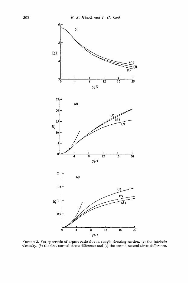
The viscosity indicates a shear thinning, as shown in figure 3 (a). The second- order-fluid approximation of a constant viscosity at low shear rates has a 5 % accuracy out to y / D = 2 . Clearly shown in the figure is the slow approach to the high-shear-rate limiting value of the viscosity of 2-85 given by Hinch & Leal (1972). It is only after y / D = 200 that the viscosity as calculated from the exact



202 E. J. Hinch and L. G. Leal

6r

I I I I I 4 8 12 16 20

Y P

YlD FIGURE 3. For spheroids of aspect ratio five in simple shearing motion, (a) the intrinsic viscosity, ( b ) the first normal-stress difference and ( c ) the second normal-stress difference.




model is within 5 yo of its limiting value. While no consideration was given to shear in the design of the approximate constitutive equations, the interpolations both have the correct qualitative behaviour, and with surprisingly good quantitative accuracy. The more sophisticated interpolation (18) is nearer to the exact results, being 3 yo out a t y / D = 10 and 4 yo out a t y / D = 20, compared with 3 yo and 7 % for (17) .

The results for the first and second normal-stress differences are shown in figures 3 ( b ) and ( c ) . Both increase quadratically with the shear rate, starting from zero, and tend to constant limiting values a t high shear rates (70.8 and 2.6, respectively). The first normal-stress difference is positive while the second is negative and less than one-tenth of the magnitude of the first. The normal stresses are a t most one-third of the size of the particle contribution to the shear stress. As with the viscosity function, the second-order-fluid asymptotics for the normal stresses hold to 5 % out to y / D = 2. There is also no sign of approach to the high-shear limits by y / D = 20. The interpolations both have the correct qualitative behaviour. The cruder interpolation (1 7) is amazingly accurate for the first normal-stress difference, within 24 % for y /D < 20, whereas the interpolation (18) has a maximum error of about 15 % for the intermediate value y / D - 10.

The behaviour of the interpolated models in steady shear flow is again surprisingly acceptable. It is true that there is some partial particle alignment in strong shear flow, especially for large aspect ratios (Leal & Hinch 1971). As we have seen, the interpolations are based on a hypothesized alignment in the strong-flow limit. Thus i t might be argued that a t least partial success is to be expected even for an aspect ratio of five. The shear viscosity, however, is not so much dependent upon the degree of particle alignment but rather is a subtle measure of the spread of the particles about their partial alignment with the flow. The normal-stress differences, which are both small compared with the shear stress, are an even more delicate measure of the skewness of the spread about alignment. The quantitative correctness of the interpolation models is therefore much more surprising than one would be led to believe on the basis of the crude argument of an averaged alignment which we have suggested above. A partial illustration of the inappropriateness of this argument can be easily obtained by simply comparing the model predictions with exact calculations for a significantly larger value of r where the degree of average alignment is increased. Such a comparison is made in figure 4, where we have plotted the viscosity and normal-stress differences for a particle aspect ratio of 25. For the viscosity, the maximum error occurs a t y / D = 20 in the range 0 < y / D < 20, and is approximately 14y0 for the interpolation model corresponding to (17), and 6 yo for (18). This comparison is actually worse than for the smaller aspect ratio, especially for the cruder interpolation (17). The behaviour of the interpolation models for the primary normal-stress difference is similar, as may be seen by comparing figures 3 ( b ) and 4 ( b ) . The maximum error for the larger aspect ratio a t y / D = 20 is approximately 25 % for interpolation (18), slightly larger than before. Finally, comparing figures 3 (c) and 4(c) for the second normal-stress difference, it can be seen that the model calculations are in somewhat poorer



204 E. J . Hinch and L. G . Leal

I I I I I I 0 4 8 12 16 20

YlD

400-

300 -

0 4 8 12 16 20

20 - 4

0 4 8 12 16 20

YlD FIQIJRE 4. For spheroids of aepect ratio twenty-five in simple shearing motion, (a) the intrinsic viscosity, ( b ) the first normal-stress difference and (c) the second normal-stress difference.




quantitative agreement for the larger aspect ratio. All of these results for an aspect ratio of twenty-five serve to emphasize the point that the greater degree of alignment which occurs with increased aspect ratio in the strong-flow limit of simple shear flow does not necessarily improve the applicability of a interpolation model which is based on a strong-flow limit with complete alignment. As we have noted earlier, the condition for strict validity of the strong-flow approximation which we have used to construct our interpolation formulae is N = O(8-6) as 8 becomes large. Simple shearing flows have N = O ( E 3 ) only.

4.4. Transients in uniaxial extension The tests of the interpolations so far have been of steady states. The dynamic viscosity will naturally be given correctly by the interpolations because they have the correct small amplitude shear behaviour built into them. A real time- dependent test must not be limited to weak flow strengths. The transient response to a suddenly imposed steady strong flow affords a suitable test. Uniaxial extension and simple shear flows have been explored.

In order to obtain some exact results for a comparison, the flow strength was made infinitely large by switching off the Brownian motion, i.e. setting D = 0. The probability equation (2) can then be bypassed using a Lagrangian method. Equation (1) must f i s t be solved and the solution expressed as p(t; po), where p = po at t = 0. Then, in the weighted integrals for the moments of N , the con- served probability may be referred back to the initial uniformly random state by

WP, W P = N(p0, Wp0 = (47Vdp0;

(PP> = IPV; P ~ ) P ( ~ ; pol (477)-ldpO.

thus, for example, in the second moment

In uniaxial extension the desired integrals can be expressed in terms of elementary functions, although the complexity of the algebra made a numerical evaluation a more attractive proposition.

The results for the transient response are shown in figure 5. The qualitative behaviour, which is correctly given by the interpolations, is a monotonic increase in the viscosity, settling down to the steady value within two strain times. The simpler interpolation (17) has a maximum error of approximately 3 % and is visually very satisfactory, while interpolation (1 8) has a maximum error of 7 % with a slight oscillation about the exact curve. To some extent, however, the more sophisticated interpolation (1 8) is only overemphasizing an interesting nonlinear effect in the exact response, in which the rate of increase of the viscosity doubles from its initial rate before decaying away.

4.5. Transients in simple shear As in the preceding subsection, the transients are for a suddenly started steady simple shear, starting from the rest state (pp) = 41 and with no diffusion, i.e. D = 0. The exact results were again obtained using a Lagrangian description.

The response of both the exact system and the interpolations is a periodic oscillation. Only when diffusion is present is the oscillation damped. Half the




I 1 I I I I 0 0.5 1 1.5 2.0 2.5 3.0

et FIGURE 5. The transients of the intrinsic viscosity in axisymmetric straining motion

for spheroids of aspect ratio five with no Brownian motion.

period is displayed in the figures. The second half of the period of the viscosity function in figure 6(a) is symmetric about the half-period, while the normal stresses in figures 6 ( 6 ) and (c) are symmetric with a sign change. The exact period of the oscillations is 16-3, compared with 15.2 for interpolation (17) and 13.5 for (18).

The oscillation in the viscosity function is a double-peaked curve with a single long trough (Hinch & Leal 1973). The starting point is in between the two peaks. The simpler interpolation (17) has the same qualitative behaviour, but with a 30 yo error. The more sophisticated interpolation (18) is much more successful, with a maximum error of only 5 %. However, the predicted period is too small by 20 yo compared with only 7 % for the simpler model.

The oscillating normal-stress differences are about one-half the magnitude of the particle contribution to the shear stress in the case of the first difference and one-eighth for the second difference. The first difference is positive in the first half-period. The second difference also starts positive but then becomes slightly negative for the majority of the half-period. Only the more sophisticated interpolation (18) has this small sign reversal in the second normal-stress difference. Otherwise the interpolations have the correct qualitative features, but errors of the order of 40 yo.

L. G. Leal wishes to acknowledge the partial support of the National Science Foundation through Grant ENG74-17590, and the Petroleum Research Fund Grant 6489-AC7, which is administered by the American Chemical Society.




2.5 -

2 -

1.5 5 0 2 4 6 8

Yt

' r

-0.5

FIUWRE 6. One-half the period of the oscillatory response to the sudden start of a simple shearing motion for spheroids of aspect ratio five with no Brownian motion: (a) the htrinsic viscosity, (a) the b t 4 normal-stress difference and ( c ) the second normal-stress difference.



208 E . J . Hinch and L. a. Leal

REFERENCES B A R ~ S - B I E S E L , D. & ACRIVOS, A. 1973 Int. J . M d t i p h e Flow, 1 , l . BRETEIERTON, F. P. 1962 J . Fluid Mech. 14,284. HAND, G. L. 1962 J . Fluid Mech. 54,423. HINCR, E. J. & LEAL, L. G. 1972 J . Fluid Mech. 52,683. HINCH, E. J. & LEAL, L. G. 1973 J . Fluid Mech. 57, 753. HINCH, E. J. & LEAL, L. G . 1975 J . Fluid Mech. 71,481. JEFFERY, G. B. 1922 Proc. Roy. SOC. A 102, 161. KBAMERS, M. A. 1946 J . Chem. Phys. 14,416. LEAL. L. G. & HINCH, E. J. 1971 J . Fluid Mech. 46,686. LEAL, L. G. & HINCH, E. J. 1973 Rheologico Acta, 12, 127. PRAGER, S. 1967 Tram. SOC. Rheol. 1,53. SCHERAGA, H. A. 1955 J . Chern. Phys. 23, 1526. SCHERAGA, H. A., EDSALL, J. T. & GADD, J. 0. 1951 J . Chern. Phya. 19,110.


Constitutive equations in suspension mechanics. Part 2. Approximate forms for a suspension of

Documents

Transcript of Constitutive equations in suspension mechanics. Part 2. Approximate forms for a suspension of