Consistent Specification Testing Via Nonparametric Series ... specification... · Consistent...
28
Consistent Specification Testing Via Nonparametric Series Regression Author(s): Yongmiao Hong and Halbert White Source: Econometrica, Vol. 63, No. 5 (Sep., 1995), pp. 1133-1159 Published by: The Econometric Society Stable URL: http://www.jstor.org/stable/2171724 . Accessed: 22/11/2013 14:19 Your use of the JSTOR archive indicates your acceptance of the Terms & Conditions of Use, available at . http://www.jstor.org/page/info/about/policies/terms.jsp . JSTOR is a not-for-profit service that helps scholars, researchers, and students discover, use, and build upon a wide range of content in a trusted digital archive. We use information technology and tools to increase productivity and facilitate new forms of scholarship. For more information about JSTOR, please contact [email protected]. . The Econometric Society is collaborating with JSTOR to digitize, preserve and extend access to Econometrica. http://www.jstor.org This content downloaded from 128.84.125.184 on Fri, 22 Nov 2013 14:19:25 PM All use subject to JSTOR Terms and Conditions
Transcript of Consistent Specification Testing Via Nonparametric Series ... specification... · Consistent...

Consistent Specification Testing Via Nonparametric Series RegressionAuthor(s): Yongmiao Hong and Halbert WhiteSource: Econometrica, Vol. 63, No. 5 (Sep., 1995), pp. 1133-1159Published by: The Econometric SocietyStable URL: http://www.jstor.org/stable/2171724 .
Accessed: 22/11/2013 14:19
Your use of the JSTOR archive indicates your acceptance of the Terms & Conditions of Use, available at .http://www.jstor.org/page/info/about/policies/terms.jsp
.JSTOR is a not-for-profit service that helps scholars, researchers, and students discover, use, and build upon a wide range ofcontent in a trusted digital archive. We use information technology and tools to increase productivity and facilitate new formsof scholarship. For more information about JSTOR, please contact [email protected].
.
The Econometric Society is collaborating with JSTOR to digitize, preserve and extend access to Econometrica.
http://www.jstor.org
This content downloaded from 128.84.125.184 on Fri, 22 Nov 2013 14:19:25 PMAll use subject to JSTOR Terms and Conditions

Econometrica, Vol. 63, No. 5 (September, 1995), 1133-1159
CONSISTENT SPECIFICATION TESTING VIA NONPARAMETRIC SERIES REGRESSION
BY YONGMIAO HONG AND HALBERT WHITE1
This paper proposes two consistent one-sided specification tests for parametric regres- sion models, one based on the sample covariance between the residual from the paramet- ric model and the discrepancy between the parametric and nonparametric fitted values; the other based on the difference in sums of squared residuals between the parametric and nonparametric models. We estimate the nonparametric model by series regression. The new test statistics converge in distribution to a unit normal under correct specifica- tion and grow to infinity faster than the parametric rate (n-1 /2) under misspecification, while avoiding weighting, sample splitting, and non-nested testing procedures used else- where in the literature. Asymptotically, our tests can be viewed as a test of the joint hypothesis that the true parameters of a series regression model are zero, where the dependent variable is the residual from the parametric model, and the series terms are functions of the explanatory variables, chosen so as to support nonparametric estimation of a conditional expectation. We specifically consider Fourier series and regression splines, and present a Monte Carlo study of the finite sample performance of the new tests in comparison to consistent tests of Bierens (1990), Eubank and Spiegelman (1990), Jayasuriya (1990), Wooldridge (1992), and Yatchew (1992); the results show the new tests have good power, performing quite well in some situations. We suggest a joint Bonferroni procedure that combines a new test with those of Bierens and Wooldridge to capture the best features of the three approaches.
KEYWORDS: Asymptotic normality for generalized quadratic forms, consistent testing, Fourier series, specification testing, regression splines.
1. INTRODUCTION
NOT LONG AFTER HAUSMAN'S (1978) landmark work on specification testing, Holly (1982) pointed out that Hausman's test fails to have unit power asymptoti- cally against a range of misspecifications of potential concern in the regression context. Beginning with Bierens (1982), numerous authors have devoted atten- tion to this problem by constructing consistent (asymptotic unit power) tests for misspecification. Particularly relevant is work of Bierens (1990), Eubank and Spiegelman (1990), Gozalo (1993), Lee (1988), Wooldridge (1992), and Yatchew (1992).
In this paper we continue this effort by proposing two new consistent one-sided specification tests for parametric regression models, one based on the sample covariance between the residual from the parametric model and the discrepancy between the parametric and nonparametric fitted values, and the other based on the difference in sums of squared residuals between the parametric and nonparametric models. Under correct specification, these two
'We wish to thank C. W. J. Granger, R. Eubank, A. R. Gallant, K. Hornik, B. Jayasuriya, S. Portnoy, Y. Rinott, P. M. Robinson, M. Stinchcombe, A. Ullah, J. Wooldridge, and two anonymous referees for helpful comments and suggestions. Any errors are attributable solely to the authors. White's participation was supported by NSF Grants SES-8921382 and SES-9209023. White also wishes to thank Robert Kunst and the Institute for Advanced Studies, Vienna, for their hospitality and support.
1133
This content downloaded from 128.84.125.184 on Fri, 22 Nov 2013 14:19:25 PMAll use subject to JSTOR Terms and Conditions

1134 YONGMIAO HONG AND HALBERT WHITE
statistics vanish faster than the parametric (nl72) rate, so a standard n1/2-nor- malization leads to degenerate test statistics. With appropriate standardization, our test statistics converge in distribution to a unit normal under correct specification and grow to infinity faster than the parametric rate under misspeci- fication, while avoiding weighting, sample-splitting, and non-nested testing pro- cedures previously used to handle the degeneracy. We estimate the nonparamet- ric model by series regressions, specifically Fourier series and regression splines. Asymptotically, our tests can be viewed as a test of the joint hypothesis that the "true parameters" of a series regression model are zero, where the dependent variable is the residual from the parametric model, and the series terms are functions of the explanatory variables, chosen so as to support nonparametric estimation of a conditional expectation. We present a Monte Carlo study comparing the finite sample performance of the new tests to tests of Bierens (1990), Eubank and Spiegelman (1990), Jayasuriya (1990), Wooldridge (1992), and Yatchew (1992); the results show that the new tests have good power, performing quite well in some situations. We suggest a joint Bonferroni proce- dure that combines our tests with those of Bierens and Wooldridge to capture the best features of the three approaches.
2. HEURISTICS
Let {Zt (Xt, YtY) R d t }= I be a sequence of i.i.d. random vectors with EIYtI < co. Then there exists a measurable function O0 such that 00(Xt) = E(YtIXt) a.s. A standard procedure to approximate QO is to specify a parametric regres- sion model, with typical element f(, a), a eA, where A is a subset of a finite dimensional Euclidean space. We are interested in testing whether the model is correctly specified for Q0, as embodied by the null hypothesis
H0: P[f(Xt ,a) = 60(Xt)] = 1 for some ao eA.
The global alternative hypothesis is
HA: P[f(Xt, a ) * O (X)] > 0 for all a eA.
Our concern here is consistent specification testing for HO against HA, i.e. testing procedures that will reject HO with asymptotic unit power whenever HO is false.
Let ain denote an estimator consistent for ao under HO; for example, ain could be the nonlinear least squares estimator, solving
n
mina=E-A n- E {Yt -f(Xt, a)}2. t= 1
We denote the fitted value fat-f(Xt, &) and the residual ?nt-Yt-fnt. A standard approach to specification testing is to regress ^nt on certain functions of the conditioning variables Xt to see if these additional regressors have any explanatory power. Under HO, they should have no such power; a joint F test
This content downloaded from 128.84.125.184 on Fri, 22 Nov 2013 14:19:25 PMAll use subject to JSTOR Terms and Conditions

CONSISTENT SPECIFICATION TESTING 1135
(asymptotically x 2) can be conducted to check this. If these additional regres- sors do exhibit statistically significant explanatory power, one has evidence of misspecification. However, such an F test will miss alternatives orthogonal to these additional regressors and is thus not consistent against HA.
We are motivated by the fact that in the presence of misspecification, the function of the conditioning variables most highly correlated with the regression error et Y, -f(X,, a *) is the specification error v, 0Q(X,) -f(X,, a *), where a * is the probability limit of an. Because E{v,e,} = E{ 00(X) - f(X, a *)}2 = 0 if and only if HO holds, a consistent test against HA can be based on the sample covariance
n
mn =n LVnt -nt , t= 1
where ?nt= Ot(Xt)-fnt and An is an appropriate nonparametric estimator of 00. Various nonparametric estimators can be used. For example, On can be the ordinary least squares series estimator, solving
n
mino E#E,-1 E {Y _0(Xt)}2, t= 1
with
/9 \ R d _ _ R a(X) = ]k, 1fJ: Rad ' Rdj
where {if,} is a sequence of basis functions, and pn is the dimension of 09, chosen to grow at an appropriate rate with the sample size n. For concreteness, we focus our attention on use of Fourier series, Gallant's (1981) flexible Fourier form (FFF), Eubank and Speckman's (1990) polynomial-trigonometric series, and regression splines.
The challenge raised by considering Mn is that for the estimators On of interest to us, the usual standardization by n1"2 is inappropriate: n M2mn
vanishes in probability under HO, a type of degeneracy. To avoid this degener- acy, Wooldridge (1992), who also considers tests based on mn, requires that the nonparametric model delivering On be incapable of nesting the parametric model, thereby inducing sufficiently slow convergence for On to 0o. Heuristically, under HO, mn can be decomposed into two dominant conflicting effects: a variance effect and a bias effect. For each sample size n, the variance diverges as Pn increases, while the bias converges to zero as Pn increases. The non-nested approach of Wooldridge (1992) uses the bias to determine the limit distribution by controlling the variance so as to be negligible. This requires a slow growth of Pn and excludes the possibility of nesting the parametric model in E9n. Otherwise, the variance will dominate the bias, leading to overrejection of H,.
A central contribution of the present work is to demonstrate that exploiting rather than avoiding the rapid convergence of tn to zero under HO leads to
This content downloaded from 128.84.125.184 on Fri, 22 Nov 2013 14:19:25 PMAll use subject to JSTOR Terms and Conditions

1136 YONGMIAO HONG AND HALBERT WHITE
statistics that diverge more rapidly under HA, with the consequent possibility of obtaining tests with better power. Our approach is to use the variance to determine the limit distribution by controlling the bias so as to be negligible. This is always possible by letting Pn grow quickly or by nesting the parametric model in &9. Consequently, we can use straightforward choices for On without having to worry about their relationship to the parametric model.
Although our approach can be applied in the presence of heteroskedastic regression errors (see Theorem A.3 in the Appendix), we focus on testing HO under homoskedasticity (i.e. E( 872X,) = o-2 a.s.) in order to keep our presenta- tion succinct. Specifically, we prove that Mn d N(O, 1) under HO, where
(2.1) Mn = (n'n /62 _P )/(2pn)1/2
where 6 2 is a variance estimator such as n-1En=1,.n2t The form taken by Mn can be understood heuristically by considering that n hn/n2 behaves asymptoti- cally like a 2 statistic. Standardization toward normality involves subtracting the mean Pn and dividing by the standard deviation (2pn) .2 As Pn -? co, the standardized quantity becomes more nearly normal. (Our proofs, however, do not rely on this heuristic, as it is a bit too simplistic.)
To get some idea of the behavior of Mn under HA, consider the case in which On is obtained using Gallant's (1981) FFF. In this case a permissible choice is Pn = ln (n). (See Theorem 3.2 below.) Because ihn tends to a positive constant under HA, Mn behaves approximately like Cn/(ln (n))l/2, where C is some constant. In contrast, Wooldridge's statistic behaves approximately like C'nl/2,
for a different constant C'. Thus, Mn diverges under HA at a rate nearly the square of that of Wooldridge's statistic.
Our second test is closely related to those of Lee (1988) and Yatchew (1992), who consider basing specification testing on
n n
tnn = n1 E en2t-n1 E %R2t, t=1 t=1
where 72nt = -On(Xt) is the residual from the nonparametric estimation. Under HO, tln converges to zero, while it will tend to a positive limit under HA, as the first term will include the specification error. Like An, 1/2 also vanishes in probability. Lee (1988) reweights 7n2t to avoid this degeneracy. Such a weighting device is sensitive to heteroskedasticity, as the test may reject HO under heteroskedasticity even when HO is true. Alternatively, Yatchew (1992) proposes splitting the sample into two independent subsets, with the first subset used to estimate the parametric model and the second subset to estimate the nonparametric model. This approach is also used by Whang and Andrews (1993, Section 5) in testing semiparametric models. As pointed out by Wooldridge (1992), sample-splitting is rather costly.
Because we view degeneracy as a virtue rather than a vice, we obtain a viable test statistic by finding the proper standardization for thn, instead of by modify-
This content downloaded from 128.84.125.184 on Fri, 22 Nov 2013 14:19:25 PMAll use subject to JSTOR Terms and Conditions

CONSISTENT SPECIFICATION TESTING 1137
ing ih0 so that the familiar n1/2-normalization is appropriate. We consider the test statistic
(2.2) Mn = (nmn/6 -p,)/(2pn)"2
and show that under HO we have Mn - Mn= op(l). That is, Mn and Mn are asymptotically equivalent. In addition to possible power improvements associ- ated with faster divergence of Mn under HA, we also avoid the drawbacks induced by weighting and sample-splitting. The statistic Mn is simple to compute because the sums of squared residuals are available in any standard regression package.
Another approach closely related to ours is taken by Eubank and Spiegelman (1990), who consider specification tests based on an orthogonal series regression using 'nt as the dependent variable. The result is a nonparametric estimator of E(,lX,); the idea is that this should be the zero function under Ho. Eubank and Spiegelman's statistic can be viewed as a joint F test using the coefficients on all the Pn included terms in the series regression. To obtain their results, Eubank and Spiegelman assume a linear model with a fixed single regressor and normally distributed errors e,. Jayasuriya (1990) generalizes Eubank and Spiegelman's results by dropping the normality assumption and permitting the linear model to be a fixed order polynomial (but still with a single fixed regressor). The tests we propose can be proven to be asymptotically equivalent to a test based on series regression with Ant as the dependent variable. Our results extend and complement those of Eubank and Spiegelman, and Jayasuriya (ES &J) by permitting nonorthogonal series, nonlinear parametric models, and random multiple regressors.
de Jong and Bierens (1991) use an approach similar to ES&J. Their test can be viewed as the heteroskedasticity-robust version of ES&J's test. Although they allow nonorthogonal series and test nonlinear parametric models, de Jong and Bierens' approach is specific to the Fourier series. Also, they show that their statistic grows at a rate of at least (n/p3/2) under HA, but do not deliver the exact rate (n/p1/2). In contrast, our approach permits such nonparametric techniques such as kernel methods and smoothing splines (see White and Hong (1993) for use of kernel methods). We are also able to deliver the exact growth rate of n/p1/2 for our test statistic under HA. Our treatment of heteroskedastic errors (Theorem A.3, Appendix) is also different from theirs.
3. SPECIFICATION TESTING WITH FOURIER SERIES AND SPLINES
We work throughout with the following data generating process (DGP).
ASSUMPTION A.1: For each n e N the stochastic process {Zt (Xt, Yt)' E +
t = 1,2 ... ., n}, d E H, is independent and identically distributed with E(Y2) <oo. The distribution ,t of X, has a continuous and positive density function p on S, where Xs is the compact support of Xt.
This content downloaded from 128.84.125.184 on Fri, 22 Nov 2013 14:19:25 PMAll use subject to JSTOR Terms and Conditions

1138 YONGMIAO HONG AND HALBERT WHITE
The bounded support assumption facilitates use of Fourier series and splines. Unbounded support could be handled with appropriate choice of series (e.g. the Hermite polynomials). With Fourier series, we need to rescale Xs to either
-[O, 2lT]d or X [v, 21T-v]d for some small v > 0. The condition on ,u is restrictive, but is not uncommon in nonparametric estimation using Fourier series methods (e.g. Andrews (1991, Section 4), Gallant and Souza (1991), and Wooldridge (1992, Example 3.1)). It implies that the Lebesgue measure is absolutely continuous with respect to u, which permits application of Edmunds and Moscatelli's (1977) results on Fourier series.
ASSUMPTION A.2: Put et Yt -E(Yt I Xt). (a) 0 < E( e2 I X,) = o2 a.s.; (b) 0 < E(4) < oo and 0 < supx E( 4Xt =x) < c-1 < oo.
The homoskedasticity assumption is a convenient but not vital condition. It greatly simplifies our test statistic. We treat the heteroskedastic case in Theorem A.3 of the Appendix. The moment condition on et helps ensure the asymptotic normality of our statistics.
Given E(Y2) <to, there exists a measurable function 00 such that 0 (Xt) =
E(YtlXt) a.s. A parametric model for 00 forms the basis of our null hypothesis.
ASSUMPTION A.3: (a) Let A be a subset of Rq, q E- N. For each n E - N the function fn: Xs XA -- R8 is such that for each a eA, fj(, a) is measurable, and fn(Xt,*) is continuous a.s. on A, with fn2(Xt ) < Dn(Xt), where Dn(Xt) is inte- grable unifornly in n; (b) for each n, fn(Xt, *) is twice continuously differentiable a.s. on A with nIVfn(Xt )112 and IV7 2fn(Xt, * )II dominated by Dn(Xt).
The dependence of fn on n will be used to generate local alternatives. Our next assumption specifies the behavior of the parametric estimator an.
ASSUMPTION A.4: { &n} is a sequence of random q-vectors such that there exists a nonstochastic sequence {a,* E int Al such that n1/2( a - a*) = Op(l).
It is not necessary to be more specific about the asymptotic behavior of a&n, as it will have no impact on the limit distribution of our test statistics. In other words, we can estimate 0o and proceed as if it were known in forming the test statistics. This greatly simplifies calculation of our test statistics. Such estimators as nonlinear least squares, generalized method of moment or adaptive efficient weighted least squares (e.g., White and Stinchcombe (1991)) estimators satisfy Assumption A.4.
To state our theorems, we define a class of local alternatives
Han: fn(Xt, a*) = 00(Xt) + (p1/4/nl/2)g(Xt),
where g is square integrable on Xs. The null hypothesis HO occurs if g = 0. As in Gallant and Jorgenson (1979) and Gallant and White (1988), we let the model
This content downloaded from 128.84.125.184 on Fri, 22 Nov 2013 14:19:25 PMAll use subject to JSTOR Terms and Conditions

CONSISTENT SPECIFICATION TESTING 1139
approach the DGP rather than vice versa. This leads to a much simpler analysis and delivers conclusions identical to those reached by fixing the model and moving the DGP appropriately.
A key consideration in constructing our tests is the number of series terms PA. To gain insight into what determines the admissible rates for pn, we decompose mn under Ho as follows:
n mln = ( en't I { ntn} (n E t et)
n + E {On*(Xd) - (Xd)}t + Op(l)
t= 1
where qint = (q(Xt),..., qip (Xt))' is a Pn X 1 vector, Tn = (ql *.*.* qinn)' is an n Xpn matrix, and On* can be viewed as solving min6 E
O E{Yt - 0(Xt)}2. The first term is a variance effect, growing as Pn ?? cc; the second term is a bias effect, vanishing as Pn ?? sufficiently fast. We use the first term to determine the limit distribution by controlling the second term to be of smaller order. For this we need to control On so that p(0n*, 0,) vanishes sufficiently fast, where P(0i, 02) -[fJ01(x) - 02(x)}21t(dx)]1l2 is an L2 norm. This can be achieved by letting Pn grow quickly or by nesting the parametric model in On. We note that mn can also be decomposed similarly, although the bias term has a different expression.
A key condition for asymptotic normality of the first term (after proper standardization and recentering) is
SUP1 < t < n (Jqnt(TnTn)_ qlnt) -P ?-
(See Theorem A.1 in the Appendix.) Since supj supx I qij(x)l < oo given our choices of { qi} specified below, a sufficient condition for this is Pn/Amin{In'tI} n 0. This restricts the growth of Pn, especially when Amin{E(T'nn/fn)} is not bounded below. (We ensure this condition by relating Amin{Tnl'n/f} to Amin{E(Tn'Tn/n)} using Gallant and Souza's (1991, Theorem 4) uniform strong law for Amin{T'n"n/f}.) Therefore, one must choose Pn properly so that the first term becomes dominant and asymptotically normal. One of our objectives is to obtain an explicit rate for Pn that implies asymptotic normality of our test statistics under H,.
We first consider nonparametric estimators based on the trigonometric series on Xs - (= [0,21.]d):
In Jn
(3.1) &n=lo - >RI0(x) = u0+ E E{uij cos(jk'x) + vij sin (k'x)) i=1 j=1
Pn A
= 3iqij(x), = 1pp(X>
where In,Jn eN,uo,uij and vij.eD, ki e KnI=-{ki: i =,...,In} is an elemen- tary multi-index, a d x 1 vector of integers (for details of the construction
This content downloaded from 128.84.125.184 on Fri, 22 Nov 2013 14:19:25 PMAll use subject to JSTOR Terms and Conditions

1140 YONGMIAO HONG AND HALBERT WHITE
of ki, see Gallant (1981)), (81(,*,9. 1.)
= (u0, 1(1)'.. (I) I(i) =(uil, ',"il, ..,uij, vaij), and the sequence {qij(x)} represents the constant function and the trigonometric functions cos(jk'x) and sin(jk'x) written in an order corre- sponding to the j8j defined above. The number of series terms is pn = 1 + 21nJn
K d, where Kn is the order of the Fourier series in (3.1). First, suppose that 00 is a periodic function defined on X that is continuously
differentiable up to order r e fiN on a subset containing X. Edmunds and Moscatelli (1977, p. 15) show that there exists a sequence {0* E 9n for En as in (3.1) such that
( o0) = O(Kn r) = Q(p-r/d).
On the other hand, Amin{E(Tn'In/n)} is bounded below given that the density p of X, is bounded away from zero on R. Applying Gallant and Souza's (1991, Theorem 4) uniform strong law for Amin{jnPn//nl, we can ensure that AminPin'Tn/nl is also bounded away from zero from below. This permits a relatively fast rate for Pn,
In stating our specification testing results, we let
n n
an = 1 E 8 ?n or - = (n i=1 t=1
where nt = -fn t n t = Yt- On(X), fnt = f(X n) and O,n =
argmin,, n- 1 En= 1{Y - 0(Xt)}2 for some appropriate On.
THEOREM 3.1: Suppose Assumptions A.1-A.4 hold and 00 is a periodic (in every coordinate) function defined on X = [0, 2 j ]d that is continuously differentiable up to order r E N on R, where 0 < r < oo. Define Mn and Mn as in (2.1) and (2.2), and
18n as in (3.1). Suppose that pn3/n -*0, p4r+d/n2d _c, where 4r 2 Sd. Then (i) under Han, M0-M0AO and
d -d Mn -N(8,1) and Mn-N(8,1),
where 8= E{g2(X)}/(2o4)12; (ii) under HA and for any sequence {Cn1, Cn =
o(nlpI12),
P[M > Cn] -1 and P[Mn > Cn] 1.
The rate pn/n -O 0 helps ensure the asymptotic normality for Mn and M,. When Xt is nonrandom, a faster rate for Pn can be obtained. The slower rates here are due to imposing the strong law on Amin{TF'<n} of Gallant and Souza (1991, Theorem 4). The rate p4r+d/n2d c, 4r> 5d, ensures that the bias p( ,n*,, 0) vanishes sufficiently fast.
Theorem 3.1 shows that consistent tests based on M6zn and m,n can be obtained without using weighting, sample-splitting and non-nested testing procedures. Besides avoiding the features associated with these approaches, a benefit of our
This content downloaded from 128.84.125.184 on Fri, 22 Nov 2013 14:19:25 PMAll use subject to JSTOR Terms and Conditions
CONSISTENT SPECIFICATION TESTING 1141
approach is that it delivers test statistics diverging under HA at a rate of lp/2,
faster than the parametric rate nl/2. (A parametric test statistic that has a null unit normal distribution typically diverges at nl/2 under the alternative.) A cost for this is that our tests can only detect local alternatives of O(p1/4/n1/2), slightly slower than n1 /2 due to Pn -? oo. However, it can be shown that this rate is still faster than the local alternatives of Lee (1988), Yatchew (1992), and Wooldridge (1992) under standard regularity conditions. In addition, our admis- sible rates for Pn are faster than those permitted by Wooldridge (1992) and Yatchew (1992). This suggests that our test may have superior power properties. We note that both our tests are one-sided, because asymptotically, negative values of our test statistics can occur only under HO. Under HA our test statistics always tend to a positive increasing number.
Of course, the periodicity of 00 is quite a restrictive assumption. Relaxing this will slow the convergence rate of the trigonometric series on S, due to the Gibb's phenomenon (boundary effects). For example, when p is uniform on [0,21T], the trigonometric series gives p(0n*,>0)=O(p,-1/2) for o0(x) = aox, x E [0, 27T]. Such a slow rate might make it difficult to have the bias negligible while maintaining asymptotic normality of our tests.
The boundary problem can be avoided and the same convergence rate maintained if we use Gallant's FFF series defined on X = [v, 2 r - V]d for some small v > 0:
( d d i (3.2) On 0: X ' R 9(x) = uo + E brxi + E E cijxixj
i=1 i=1 j=1
In Jn Pn
+ E {uij cos(jk'x) + vij sin(jk'x)} = E, I38ij(x)E, i=1 j=1 j=1 J
where (I3l,../3Pn)=(uo,?3(), I3(1)*._,I3(I )), P(O) =8(bl *1,..., bdcllc12...cdd)
Aw i = 1,..., Jn, is as in (3.1), and the sequence {qij(x)} now includes a constant, xi, xixi, and cos (jk'x) and sin (jkIx) written in an order corresponding to the A key difference of On in (3.2) from On in (3.1) is that On in (3.2) is defined on X= [v, 27r - v]d, which does not include the boundary. As pointed out by Gallant and Souza (1991), inclusion of xi and xixj helps improve finite sample performance and provides a means to test economic hypotheses. The same convergence rate is still obtained if only trigonometric series are included in (3.2).
If 00 is continuously differentiable up to order r on a subset containing X, then there exists a periodic function defined on S = [0, 27T ]d that is continuously differentiable up to r order on a subset containing X and coincides with 00 on X. As pointed out by Gallant (1981), Edmunds and Moscatelli's (1977) results can be applied to show that there is a sequence {o* E,- an} such that the same convergence rate is obtained as in the periodic case. A problem arises here
This content downloaded from 128.84.125.184 on Fri, 22 Nov 2013 14:19:25 PMAll use subject to JSTOR Terms and Conditions

1142 YONGMIAO HONG AND HALBERT WHITE
because Amin{E(V'n`n/n)1 is not bounded below for the FFF series on X. (The same is true if E, in (3.2) does not include xi and xr xj.) Gallant and Souza (1991, Section 5) show that for the FFF series on SS, Amin{E(Tn'Pn/n) =
o(Pn (S+e)/d) for every s E- N and every 8 > 0. Thus, it appears that Amin{,I'Pn/nl vanishes rapidly. This restricts the growth of Pn. Given such a slow growth of p, this also restricts the class of 00 that permits quick reduction of the bias P(On, Q).
THEOREM 3.2: Suppose Assumptions A.2-A.4 hold and that 00 is continuously differentiable of order o on a subset containing X = [ ', 2ir - 1 ]d for some small v > 0. Define Mn and Mn as in (2.1) and (2.2), and En as in (3.2). Suppose pn is such that a(pn/d)ln(pl/d) < ,13 ln(n) for some 0 < , < 1/2 and some increasing function a: IR + R+ with limp a(p / d) = oo. Then (i) under Han, Mn -M *n 0 and
d -d Mn -N( 8, 1) and Mn -N( 8, 1);
(ii) under HA and for any sequence {Cn), Cn n
P[Mn > Cn] ->1 and P[AMn > Cn 1-*i'
We thus relax the periodicity assumption of 0Q at the cost of increasing smoothness and slowing the rate for Pn. As discussed in Gallant and Souza (1991, Section 5), a(pn/d)ln(pl/d) < /3 ln(n) implies that nY/Pn -*oo for any Y > 0, SO Pn can only grow at a rate slower than any fractional power of n. For example, if we take a(p /d) = 8 ln(n)/ln(p /d), then p0 ln(n). Because under HA our statistics diverge at a rate of n/pll2, it follows that the slower P0 is, the faster our statistics grow asymptotically. With Pn = ln (n), our statistics grow at almost the square of the parametric rate (n1/2). Of course, the slow rate for Pn may adversely affect the finite sample performance of our tests when the sample size is not sufficiently large.
To obtain a faster rate for pn, an alternative to ensure that the bias vanishes under HO is to nest the parametric model in the nonparametric specification. While this approach is applicable to nonlinear parametric models, we focus for simplicity on linear models. We consider the FFF series on the cube S:
(3.3) E9n is as defined in (3.2) with x = [0, 2r ]d replacing X = [2v,2 - v]d.
Now Amin{E(Ii'tn/n)1 of the FFF series on SS vanishes only at a polynomial rate. Direct calculation shows that if the density p is bounded below, then Amin{E(Vn'tn/n)} = Q(p,-3/d). (The rate Q(pnl/d) appearing in Gallant and Souza (1991) is a typo.) Hence, a faster rate for Pn is obtainable. In fact, if we choose
(3.4) On is as defined in (3.3) with ci = 0 for all i,] = 1,..., d,
This content downloaded from 128.84.125.184 on Fri, 22 Nov 2013 14:19:25 PMAll use subject to JSTOR Terms and Conditions

CONSISTENT SPECIFICATION TESTING 1143
i.e. a combination of the trigonometric series with linear terms xi only, then an even faster rate for pn can be obtained because for En in (3.4), Amin{EQI',I/f)} = Q(p-1/d). We give a formal result as follows.
THEOREM 3.3: SupposeAssumptionsA.l-A.2 hold and E(XtX) is nonsingular. Let fn(Xt, a) =Xt'a + (p1/4/nt/2)g(Xt) for a E int A, where A is a subset of Rq, q E RN, and g is square integrable with E{Xtg(xt)} = O. Let a,n =
argmin,,E A n-1 n= 1(Y -Xta )2. Define Mn and MAn as in (2.1) and (2.2), and either (a) E9n is as in (3.3) with Pn = o(nd/3(d+2)) or (b) On is as in (3.4) with pn = o(nd/(3d+2)). (i) Suppose 0Q(X,) =Xtao a.s. for some ao E int A. Then Mn-JMn 4 0, and
Mn -*N(8,1) and MAn ,N(8,1);
(ii) suppose 00 is square integrable on X with respect to ,u. Then under HA and for any nonstochastic sequence {Cn}, Cn =o(nlpn/2)
P[Mn > Cn- 1 and P[M > Cn -)1.
For both E, as in (3.3) and (3.4), admissible rates for Pn are faster than those permitted by On in (3.2). This approach also applies to testing fixed order polynomial models by extending 0n in (3.3) to include the null polynomial model. One can expect that the rates for P, will be adversely affected by the order of polynomial model.
Both (3.3) and (3.4) belong to Eubank and Speckman's (1990) polynomial-trig- onometric series. As pointed out by Eubank and Speckman, this series fits better than the pure trigonometric series on SS because the (low order) polynomials alleviate the boundary effects. Since ES&J's tests can be shown to be asymptoti- cally equivalent to our tests when the series used for our tests does not include the null linear model (Hong and White (1991, Theorem 2.6)), we also expect that the tests of Theorem 3.3 may have better power than ES&J's tests. This is investigated in our simulation.
Although En as in (3.4) permits a faster rate for Pn than En as in (3.3), this does not necessarily imply that (3.4) will give better power in finite samples, because under HA, 0n as in (3.3) may fit 0,, better. By Eubank and Speckman (1990, Theorem 4.1), when 0, is twice continuously differentiable, E,n as in (3.3) could fit 0,, better asymptotically than 0, as in 3.4 in terms of mean squared error if the optimal pn is chosen. We compare these two series in the simula- tion.
Finally, we turn to regression splines. For notational simplicity, we consider only the single regressor case, with X- [0,1]. Let A = {silit 1 with 0 = s, < ...
< Sq+ 1 = 1 be a partition of X, into q subintervals
Ij= [Si,S+l), j= 1, ... ,q-1 and Iq=[Sq,Sq+1].
This content downloaded from 128.84.125.184 on Fri, 22 Nov 2013 14:19:25 PMAll use subject to JSTOR Terms and Conditions

1144 YONGMIAO HONG AND HALBERT WHITE
Let h be the mesh size and s E N. Then the space of polynomial splines of order s with simple knots s,...., Sq can be defined as
&(s,q, A)
={0: XBs 'R 0(x) =pj(x) for x E Ij, where pj(x) is a sth order
polynomial such that pj(x) is Cs-2 at knot sj, j = 1...q}.
The dimension of &(s, qn, zn) is Pn- s + qn. Let {ijj(x)}, j = 1,... ., pnS be a basis spanning 0(s, qn, An). Then 0(s, qn, An) can be written as
Pn
(3.5) 0(s(5 qn 7 /n) 0: X s -->R 0 (X) = pj ,Bytj(x), tjj: X5s-- R, j8j E= Ri
It is well known (e.g., Schumaker (1981, Theorem 6.42)) that for any 0Q that is continuously differentiable up to order r on a subset containing Xs, there exists a sequence {On E O(s,pPnS,n)} such that if r<s, p(Qn ,)==Q(pr). Thus, p4r+ '/n2 oo 0 suffices to ensure that the bias effect vanishes quickly under H
When r > s and 0Q is not a polynomial of order s or less, p(O*, 0) (p-s), due to the "saturation effect" of the polynomial splines. In this case, p45+ I/n2
oo suffices.
A convenient choice for {(ql) is the normalized sth order B-spline {Njs} associated with knots si,... sj+S that satisfy the so-called partition of unity property, i.e. for all s ? 1 and j = 1,..., Pn
E: NJs(x) = for all sj <x <sj + . i=j+ 1 -s
From this we have 0 < Nis(x) < 1 for all x E Xs and all j. For more detailed discussion of Njs(X), see e.g. Schumaker (1981, Ch. 4).
Put Nns, (Njs(X1),..., Ns (Xt))'. Then Amin(ENnstNns,) is not bounded below. In the case of equally spaced knots with spacing hn l/p, = hn and s given, it can be shown that n 1 I lE(Nnsr Nns,) is a block-diagonal Pn X Pn symmetric matrix with Amin(ENnrNn) - 0(P )) Again, this restricts the growth Of Pn.
THEOREM 3.4: Suppose Assumptions A.1-A.4 hold and 00 is continuously differentiable up to order r e N on a subset containing Xs = [0, 1]. Define Mn and Mn as in (2.1) and (2.2) and En- -n(s, qn, A,n) as in (3.5) with hn 1/pln and
{qfj} = {Njs}, the normalized sth order B-spline. Suppose either (a) 3 < r < s, p4r+ 1/n2_ , p5/n or (b) r>s3, p4s+ l/n2 o, p5/n- 0. Then (i)
under Han, Mn -Mn ` 0, and
d -M ( , 1); Mn -->N( &~1) and Mn N(c3,1N
This content downloaded from 128.84.125.184 on Fri, 22 Nov 2013 14:19:25 PMAll use subject to JSTOR Terms and Conditions

CONSISTENT SPECIFICATION TESTING 1145
(ii) under HA and for any sequence {CnJ, Cn = n
P[Mn > Cn]- 1 and P[Mfn > Cn ] 3.
For unequal spacing, this result still holds if the spacing is appropriately chosen.
4. MONTE CARLO EVIDENCE
We compare the finite sample performance of our tests to consistent tests of Bierens (1990), ES&J, Wooldridge (1992), and Yatchew (1992) using Monte Carlo methods. Each test statistic is asymptotically unit normal under Ho, and except for Bierens' test, all are one-sided. We examine both size and power by testing correct specification for E(YIX,) of a linear model against a number of alternatives.
Four DGP's are produced using the Gauss 386 random number generator:
DGP1: Yt=1+Xjt+X2t+et=XtAa0 + 8t
DGP 2: Yt =Xtlao + 0.1(Vlt - ')(V2t - 7) + et,
DGP 3: Yt = Xt'ao + Xt'ao exp -0.01(Xt'ao) 2}? + et
DGP 4: Yt = (xt;a0) -05 + Et,
where X1t = (Vt + V1t)/2, X2t = (Vt + V2t)72, Vt, Vlt, and V2t are i.i.d. U[0,2T], and Et is i.i.d. N(0, o-02) with o2 = 1 or 4. A linear model fn(Xt, a) =Xt'a a0 + a1X1t + a2X2t is correctly specified for E(YtlXt) under DGP 1 and misspeci- fied under DGP's 2-4. DGP 2 originates from the alternative used by Bierens (1990), except that Vt, V1t and V2t are drawn from i.i.d. U[0,21T] instead of i.i.d. N(0, 1). DGP 3 is similar to the alternative used by Eubank and Spiegelman (1990); and DGP 4 is one of the alternatives used by Wooldridge (1992).
Bierens' test involves choosing an increasing number of values of a nuisance parameter T and a penalty term yn ', where y > 0, 0 < p < 1. We draw T from a uniform distribution on [1, 5]2, choose (n/10) - 1 for the number of T's, and use two penalty rules: (y, p) = (0.25, 0.5) and (0.25, 0.25).
Two nonparametric series are used for our tests of Theorem 3.3: a quadratic- trigonometric (QT) series with Pln = [n 015 ln (n)], and a linear-trigonometric (LT) series with Pn = [n024 lnn(n)], where [a] denotes the integer closest to the real number a. These rates, given d = 2, satisfy the conditions of Theorem 3.3. Since both series include a linear model and a,n is estimated by OLS, Mn and Mn are numerically identical, as is easily verified. Therefore, we need not distinguish them. The above two series with their rates are also applied to Yatchew's test with equal sample-splitting. For our tests, we use 2
(n -p)1)I2> to estimate T Use of A_ n- nEtn gives similar results, with slightly less power. (See Hong and White (1991).) For Yatchew's test, we
This content downloaded from 128.84.125.184 on Fri, 22 Nov 2013 14:19:25 PMAll use subject to JSTOR Terms and Conditions

1146 YONGMIAO HONG AND HALBERT WHITE
use gnt to form an estimator for var (t2). Use of 7 to form an estimator for var(6t2) leads to strong overrejection.
For our multivariate version of ES&J's tests, a pure trigonometric series without the constant is used to satisfy the appropriate conditions. For compari- son with our tests, we also choose Pn = [n?15 ln (n)] and [n0.24 ln (n)] for ES&J's tests and use numerically identical estimators for To20
The QT or LT series estimator is prohibited in Wooldridge's non-nested test. Like Wooldridge, we use a trigonometric series with a constant. We use two rates: Pn = [In (n)] and Pn = 5, 7, 9 for n = 100, 300, 500 respectively. The latter is used by Wooldridge.
We use the following notations: NEW1 and NEW2 denote our tests with the QT and LT series estimators respectively; BT1 and BT2 denote Bierens' tests with (-y, p) = (0.25,0.5) and (0.25,0.25) respectively; ESJ1 and ESJ2 denote ES&J's test with pn = [n015 ln(n)] and [n024 ln(n)] respectively; WT1 and WT2 denote Wooldridge's test with pn = [ln (n)] and pn = 5, 7, 9 for n = 100, 300, 500, respectively; and finally, YT1 and YT2 denote Yatchew's tests with the QT and LT series estimators respectively.
All the tests are based on the same seeds and 1000 replications, with a different seed for each n. We use both the asymptotic critical value (ACV) and the empirical critical value (ECV) at the 5% level. The ECV's are generated using 5000 replications, and are reported in Table I. In all cases, the ECV's of our tests and those of ES &J are less than 1.65, the 5 % ACV. This differs from the finding of ES &J, who report an ECV larger than 1.65 for the classical linear model with a single fixed regressor and n = 100. We first examine size. Table II shows rejection rates using both the ACV and ECV of all test statistics under DGP 1. In all cases, our tests are conservative, and so are ES&J's tests. BT1 has reasonable size, but BT2 has a tendency toward overrejection. This warns against choosing too small a penalty for Bierens' test. WT1 and YT1 exhibit some overrejection; WT2 and YT2 exhibit strong overrejection, i.e., the faster Pn grows, the stronger the overrejection. Therefore, both Wooldridge and Yatchew's tests exhibit potential "overfit" problems when Pn grows too fast. In contrast, our tests are still conservative even if Pn grows faster than the rates permitted by Theorem 3.3 (not reported here). When To2 increases, all the tests except Wooldridge's tests remain unchanged; Wooldridge's tests become worse.
Tables Ill-V report power performances under DGP's 2-4. Under DGP 2, misspecification of a linear model is "small" in the sense that the neglected nonlinearity is uncorrelated with Xt; the OLS estimator a,n is consistent for ao. Our tests and ES&J's tests are powerful against DGP 2. NEW1 is a little more powerful than NEW2, i.e. the QT series performs better than the LT series, although the rate of pn for the QT series is slower. BT1 and BT2 have some power, but are much less powerful than our tests and those of ES&J. WT1, YT1, and YT2 have little power against DGP2. WT2 gains power when n = 500 and 0To=2 4. When o02 increases, the power of most tests suffers, but the ranking of relative performances of all the tests remains unchanged.
This content downloaded from 128.84.125.184 on Fri, 22 Nov 2013 14:19:25 PMAll use subject to JSTOR Terms and Conditions
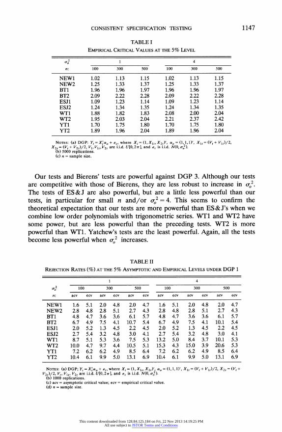
CONSISTENT SPECIFICATION TESTING 1147
TABLE I
EMPIRICAL CRITICAL VALUES AT THE 5% LEVEL
?o2 1 4
n: 100 300 500 100 300 500
NEW1 1.02 1.13 1.15 1.02 1.13 1.15 NEW2 1.25 1.33 1.37 1.25 1.33 1.37 BT1 1.96 1.96 1.97 1.96 1.96 1.97 BT2 2.09 2.22 2.28 2.09 2.22 2.28 ESJ1 1.09 1.23 1.14 1.09 1.23 1.14 ESJ2 1.24 1.34 1.35 1.24 1.34 1.35 WT1 1.88 1.82 1.83 2.08 2.00 2.04 WT2 1.95 2.03 2.04 2.21 2.37 2.42 YT1 1.70 1.75 1.80 1.70 1.75 1.80 YT2 1.89 1.96 2.04 1.89 1.96 2.04
NOTES: (a) DGP: Y, = X;a0 + c,, where XI = (1, X1I, X21)', aO = (1,1,1)', X1 = (V, + V1t)/2, X2 = (Vt + V2t)/2, V1, Vlt, V2, are i.i.d. U[0, 2 7r1, and et is i.i.d. N(0, o-2).
(b) 5000 replications. (c) n = sample size.
Our tests and Bierens' tests are powerful against DGP 3. Although our tests are competitive with those of Bierens, they are less robust to increase in or2.
The tests of ES&J are also powerful, but are a little less powerful than our tests, in particular for small n and/or cr,2 = 4. This seems to confirm the theoretical expectation that our tests are more powerful than ES&J's when we combine low order polynomials with trigonometric series. WT1 and WT2 have some power, but are less powerful than the preceding tests. WT2 is more powerful than WT1. Yatchew's tests are the least powerful. Again, all the tests become less powerful when cr 2 increases.
TABLE II
REJECTION RATES (%) AT THE 5% ASYMPTOTIC AND EMPIRICAL LEVELS UNDER DGP 1
1 4
0-o2 100 300 500 100 300 500
n: acv ecv acv ecv acv ecv acv ecv acv ecv acv ecv
NEW1 1.6 5.1 2.0 4.8 2.0 4.7 1.6 5.1 2.0 4.8 2.0 4.7 NEW2 2.8 4.8 2.8 5.1 2.7 4.3 2.8 4.8 2.8 5.1 2.7 4.3 BT1 4.8 4.7 3.6 3.6 6.1 5.7 4.8 4.7 3.6 3.6 6.1 5.7 BT2 6.7 4.9 7.5 4.1 10.7 5.4 6.7 4.9 7.5 4.1 10.1 5.4 ESJ1 2.0 5.2 1.3 4.5 2.2 4.5 2.0 5.2 1.3 4.5 2.2 4.5 ESJ2 2.7 5.4 3.2 4.8 3.0 4.1 2.7 5.4 3.2 4.8 3.0 4.1 WT1 8.7 5.1 5.3 3.6 7.5 5.3 13.2 5.0 8.4 3.7 10.1 5.3 WT2 10.0 4.7 9.7 4.4 10.5 5.1 15.3 4.3 15.0 3.9 20.6 5.3 YT1 7.2 6.2 6.2 4.9 8.5 6.4 7.2 6.2 6.2 4.9 8.5 6.4 YT2 10.4 6.1 9.9 5.0 13.1 6.9 10.4 6.1 9.9 5.0 13.1 6.9
NOTES: (a) DGP; Y,
= X'ao
+ c,,
where X4 = (1, X1t, X2)', YaO
= (1, 1, 1)', X1 = (Vt + V1t)/2, X2 = (Vt + V2t)/2, Vt, V1t, V2, are i.i.d. U[0,27r], and et is i.i.d. N(O, o).
(b) 1000 replications. (c) acv = asymptotic critical value; ecv = empirical critical value. (d) n = sample size.
This content downloaded from 128.84.125.184 on Fri, 22 Nov 2013 14:19:25 PMAll use subject to JSTOR Terms and Conditions

1148 YONGMIAO HONG AND HALBERT WHITE
TABLE III
REJECTION RATES (%) AT THE 5% ASYMPTOTIC AND EMPIRICAL LEVELS UNDER DGP 2
1 4
0-",2 100 300 500 100 300 500
n: acv ecv acv ecv acv ecv acv ecv acv ecv acv ecv
NEW1 32.2 46.5 85.2 91.6 99.4 99.9 7.5 13.7 17.5 26.5 37.2 49.9 NEW2 28.1 36.8 75.1 81.5 96.2 97.9 8.6 12.4 12.0 19.5 28.6 35.1 BT1 12.3 12.1 31.6 31.6 49.3 48.7 6.9 6.9 9.9 9.9 16.9 16.6 BT2 16.0 10.5 42.8 31.3 42.8 31.3 8.2 6.4 16.8 9.9 27.1 17.4 ESJ1 30.5 43.8 83.4 88.9 98.6 99.5 7.0 12.3 17.2 24.5 37.2 48.7 ESJ2 26.4 36.2 72.9 79.1 95.8 97.6 8.0 11.7 13.9 19.4 27.3 35.5 WT1 9.3 6.2 5.7 2.8 10.1 5.3 13.3 4.9 7.8 3.0 8.1 5.9 WT2 9.3 4.7 9.9 4.1 20.6 5.3 14.8 3.7 16.2 4.2 82.6 70.3 YT1 9.9 8.6 11.3 9.3 19.7 14.4 8.1 7.4 7.2 6.0 9.7 7.9 YT2 14.2 8.4 18.0 10.4 27.5 14.2 11.0 6.6 11.2 5.8 15.6 7.8
NOTES: (a) DGP: Y, = X;a0 + 0.1(V1, - 7rXV2,- 7r) + et, where X2 = (1, X1t, X2t)', O = (1, 1,1)', X1 =
(Vt+ Vit)/2, X2,= (Vt+ V2d)/2, Vt,V1t,V2, are i.i.d. U[0,27r1, and et is i.i.d. N(O, o). (b) 1000 replications. (c) acv = asymptotic critical value; ecv = empirical critical value. (d) n = sample size.
Interestingly, WT1 and WT2 are the only tests that have some power against DGP 4. When oC,2 increases, they become slightly less powerful at the ECV. All other tests do not have power against this DGP.
To summarize our findings: (i) The sizes of our tests are conservative and robust to increase in or2; so are ES&J's tests. Bierens' test has a reasonable size when the penalty term is not chosen too small. The tests of Wooldridge and Yatchew may overreject when the nonparametric estimator "overfits" the data.
TABLE IV
REJECTION RATES (%) AT THE 5% ASYMPTOTIC AND EMPIRICAL LEVELS UNDER DGP 3
1 4
0-02 100 300 500 100 300 500
n: acv ecv acv ecv acv ecv acv ecv acv ecv acv ecv
NEW1 79.6 86.9 99.9 100.0 100.0 100.0 17.1 28.0 60.7 71.1 86.9 92.7 NEW2 73.0 80.2 99.9 100.0 100.0 100.0 14.9 21.4 50.6 59.5 86.0 92.2 BT1 87.9 87.9 100.0 100.0 100.0 100.0 38.7 38.6 83.7 83.7 96.5 96.4 BT2 93.2 91.6 100.0 100.0 100.0 100.0 49.3 43.0 93.5 88.9 99.3 98.0 ESJ1 70.9 79.8 99.9 99.9 100.0 100.0 12.8 22.8 50.4 61.3 78.3 86.8 ESJ2 64.7 73.8 99.6 99.8 100.0 100.0 13.6 20.0 47.1 54.9 73.3 79.9 WT1 44.2 36.8 71.9 65.3 88.8 84.1 32.5 19.5 42.0 29.3 56.9 43.5 WT2 42.0 29.7 92.8 87.2 99.4 99.0 32.1 15.4 67.0 38.4 85.7 65.2 YT1 16.1 14.1 27.6 24.1 44.5 38.5 9.0 7.5 9.8 8.2 14.3 11.2 YT2 23.4 14.2 37.6 24.0 54.9 36.1 13.5 7.7 14.8 7.8 21.7 10.7
NOTES: (a) DGP: Y, = Xcao + (XMad)exp {- 0.01(Xa0)2) + et, where X4 = (1, X1t, X2)', ao = (1, 1, 1)', Xt = (Vt + V1t)/2, X2 = (Vt + V2t)/2, V1, Vlt, V2, are i.i.d. U[0,27r], and et is i.i.d. N(0,1o).
(b) 1000 replications. (c) acv = asymptotic critical value; ecv = empirical critical value. (d) n = sample size.
This content downloaded from 128.84.125.184 on Fri, 22 Nov 2013 14:19:25 PMAll use subject to JSTOR Terms and Conditions

CONSISTENT SPECIFICATION TESTING 1149
TABLE V
REJECrION RATES (%) AT THE 5% ASYMPTOTIC AND EMPIRICAL LEVELS UNDER DGP 4
1 4
2f 100 300 500 100 300 500
n: acv ecv acv ecv acv ecv acv ecv acv ecv acv ecv
NEW1 1.6 5.4 2.2 5.0 2.5 5.2 1.6 5.3 2.2 4.7 2.2 4.8 NEW2 3.1 5.4 2.6 5.2 3.1 4.8 2.8 5.0 2.6 5.3 2.7 4.7 BT1 4.4 4.8 4.6 4.6 7.9 7.8 4.8 4.8 4.1 4.1 6.8 6.4 BT2 6.5 5.1 9.4 4.7 12.9 7.1 6.6 4.9 8.9 3.7 11.5 5.6 ESJ1 2.1 5.3 2.0 4.6 2.6 5.1 2.0 5.3 1.9 4.6 2.3 4.8 ESJ2 2.7 5.7 3.0 5.3 3.4 4.9 2.7 5.4 2.9 5.0 3.1 4.3 WT1 31.3 19.8 38.1 30.8 50.8 40.9 30.8 14.1 38.7 22.3 52.7 32.0 WT2 38.6 22.9 65.3 43.6 85.5 67.9 38.3 14.8 66.2 27.0 85.7 46.8 YT1 7.5 6.5 6.2 5.0 8.5 6.2 7.5 6.3 6.0 4.9 8.5 6.4 YT2 10.2 6.2 9.9 5.2 13.3 6.9 10.3 6.2 9.8 5.0 13.0 6.9
NOTES: (a) DGP: Y, = (X;,a )-0.5 + e,, where X, = (1, X1t, X2z)', aO = (1, 1, 1)', X1i = (Vt + V1t)/2, X2t
(Vt + V2t)/2, V,, V1, V2, are i.i.d. U[0, 27r, and et is i.i.d. N(0, o-9
(b) 1000 replications. (c) acv = asymptotic critical value; ecv empirical critical value. (d) n = sample size.
(ii) Our tests are powerful in some cases. They are often a little more powerful than ES&J's tests, and much more powerful than Yatchew's test. They are also competitive with or more powerful than Bierens's test. (iii) No one test domi- nates the others in power. (iv) The powers of all the tests suffer from increase in
2, as should be expected. Because no one test dominates the others, we explore the extent to which
combining these tests can capture the best features of each. We use a simple Bonferroni procedure, which gives an upper bound on the joint p-value of several test statistics despite their possible dependence. Let P1, ... . Pk be the ordered p-values corresponding to k test statistics, with P1 being the smallest. The Bonferroni procedure says to reject Ho at level a if P1 < a/k.
Table VI reports the rejection rates of some Bonferroni procedures with various combinations of the above tests. We first consider a procedure combin- ing all the tests. Bonferroni 1 combines NEW1, BT1, ESJ1, WT1, and YT1. The reason for choosing BT1, WT1, and YT1 is to avoid possible overrejections. This procedure has a reasonable size and is powerful against DGP's 2-3. It has a little power against DGP 4. Because Yatchew's tests are always dominated by some other test, we drop YT1 in obtaining Bonferroni 2, which now consists of NEW1, BT2, ESJ1, and WT1. There are some improvements in power, in particular against DGP 4. Since NEW1 is slightly more powerful than ESJ1 against DGP's 2-3, we drop ESJ1 in obtaining Bonferroni 3, which consists of NEW1, BT1, and WT1. There are again some improvements in power against DGP 4, with reasonable size. We also report Bonferroni 4, consisting of BT1, ESJ1, and WT1. It is slightly less powerful than Bonferroni 3. Of the four procedures, we prefer Bonferroni 3.
This content downloaded from 128.84.125.184 on Fri, 22 Nov 2013 14:19:25 PMAll use subject to JSTOR Terms and Conditions

1150 YONGMIAO HONG AND HALBERT WHITE
TABLE VI
REJECTION RATES (%) OF BONFERRONI PROCEDURES AT THE 5% ASYMPTOTIC LEVELS
2 1 4
DGP n: 100 300 500 100 300 500
1 Bonferroni 1 4.0 3.1 5.1 5.1 3.6 6.1 Bonferroni 2 3.6 3.0 4.7 5.1 3.3 5.6 Bonferroni 3 4.6 3.2 6.1 6.1 4.4 7.3 Bonferroni 4 4.4 3.3 5.9 5.9 4.5 7.1
2 Bonferroni 1 26.3 79.8 98.3 7.8 15.6 33.9 Bonferroni 2 27.3 81.1 98.5 8.3 16.6 34.7 Bonferroni 3 27.1 80.3 98.4 9.6 16.7 33.6 Bonferroni 4 25.0 76.2 97.6 9.1 16.2 32.0
3 Bonferroni 1 81.7 99.9 100.0 27.5 70.7 93.3 Bonferroni 2 82.5 99.9 100.0 29.2 73.4 94.0 Bonferroni 3 84.8 99.9 100.0 33.1 76.1 94.2 Bonferroni 4 81.8 99.9 100.0 31.9 74.4 93.7
4 Bonferroni 1 9.4 12.3 21.2 9.8 13.4 19.6 Bonferroni 2 10.5 14.3 23.9 10.5 14.9 23.2 Bonferroni 3 12.9 19.3 27.8 12.5 18.1 28.9 Bonferroni 4 12.9 19.3 27.7 12.6 18.1 28.8
NOTES: (a) Bonferroni 1 is a Bonferroni procedure consisting of NEW1, BT1, ESJ1, WT1, and YT1; Bonferroni 2 consists of NEW1, BT1, ESJ1, and WT1; Bonferroni 3 consists of EW1, BT1, and WT1; Bonferroni 4 consists of ESJ1, BT1, and WT1.
(b) 1000 replications.
5. CONCLUSION AND DIRECTIONS FOR FURTHER RESEARCH
This paper proposes two consistent specification tests for nonlinear paramet- ric models via nonparametric series regressions. The test statistics grow at a rate faster than the parametric rate under misspecification, while avoiding weighting, sample-splitting and non-nested testing procedures previously used in the litera- ture. Our approach can be viewed as a nested testing complement to Wooldridge's (1992) non-nested testing approach. It permits more flexible non- parametric estimation. Our results suggest possibly better size and better power in finite samples, as confirmed by simulation experiments, which also compare the relative performance of some related consistent tests. We examine a Bonferroni procedure to capture the best features of several alternative tests.
While our results are stated under the homoskedasticity assumption, our approach applies to heteroskedastic errors as well, with proper modification of the test statistics (see Theorem A.3 in the Appendix). Furthermore, our treat- ment of degenerate statistics is not restricted to regression contexts and to the two statistics studied here. For example, because of its appealing intuitive interpretation, relative entropy has been proposed and used to test certain interesting nonparametric hypotheses (e.g. Robinson (1991)). Since the nonpara- metric entropy estimator also vanishes faster than the parametric rate under the null hypothesis, our approach can be used to derive a well-defined distribution,
This content downloaded from 128.84.125.184 on Fri, 22 Nov 2013 14:19:25 PMAll use subject to JSTOR Terms and Conditions

CONSISTENT SPECIFICATION TESTING 1151
thus providing an alternative to the weighting device previously used in the literature. See Hong and White (1995) and White and Hong (1995) for details.
Dept. of Economics, Cornell University, Uris Hall, Ithaca, NY 14853, U.S.A. and
Dept. of Economics, University of Califomia-San Diego, 9500 Gilman Dr., La Jolla, CA 92093, U.SA.
Manuscript received January, 1992; final revision received November, 1994.
MATHEMATICAL APPENDIX
We first state and prove Theorems A.1-A.2. Theorems 3.1-3.4 then follow as corollaries of Theorem A.2. Theorem A.3 treats heteroskedastic errors. First, we state the following conditions:
AssuMPTION B.: 0, = {8: 8(x) = "n ' /3. ir(x), e/3; e R8 and 1ji: Rd ) is such that (a) n'Pn is nonsingularfor all n sufficiently large a.s.; (b) SUpM VP)1 0int ? as.; (c) there exists a sequence {(n* e &n} such that P(E, o f90) -?(pn/4/n'/2) underHe, and P(O,* 6o) =
o(1) under HA.
ASSUMPTION B.2: 6n2 is measurable such that ,2 - = ?p( p, n _2) underH and 52 - n*2 op(l) under HA for some ,n*2, n< c < *2<c- < 0, n= 1,2.
THEOREM A.1: Suppose Assumptions A.1-A.2 and B.1(a, b)-B.2 hold. Define W =
{Et et i'nt{nI'4nI}' {Et nt te)}. Let pn -? ?o as n -+ oo. Then (Wn/5n2 -pn)/(2p)"'2 - N(O,1) .
PROOF: Throughout this Appendix, we denote E, = En, 1, ESE < t = En= 2Es=1, EEk <0< = En _-1s En -t-11~-'s#1 L
Et= 3Es2k-1 and EEEEi < k < s < t = 4=Et-3k 2Ei1 For notational simplicity and without loss of generality, we set 0.n2 - 1. Put p,, / t An- Ent,Pnpe,2-Pn and U,, EEs < tUnts, where Unts, 2st tnt pns es Then Wn =pn + Un +An . We first show that Pn- '/2A, = op(l). Given Assumptions A.1-A.2 and the identity Et, nt Pnt =pPn, we have E(An) = 0 and
E(An = E{ (,Pnt t(S,2 1)}
=E E E(pn,t(pnt)((Pns(pns)E[(et2 _1)( es2 _1) IXI,.. Xn ] t s
=EE ( pn,t ,pnt)2E[(t2 _ 1)2IXl,.x.,Xn* ** E ] ?c ( 'En( t q,pnt)2 t t
< c-1 pn E bsup(envts neti t
Hence,Pn- 1 /A = op(l) by Chebyshev's inequalitygiven Assumption B.l1(b). Therefore,
This content downloaded from 128.84.125.184 on Fri, 22 Nov 2013 14:19:25 PMAll use subject to JSTOR Terms and Conditions

1152 YONGMIAO HONG AND HALBERT WHITE
We next consider U,,. Because E(U,t,IZt) = E(U,t,IZ5) = 0 for t 0 s, where Zt = (Yt, Xt)', Lemma 2.1 of de Jong (1987) holds and we can use his CLT's for generalized quadratic forms. By de Jong (1987, Proposition 3.2), Un/Sn 4 N(0, 1) if GI, GI,, and GIv are o(S4), where S= EUn2, and
GI E Un4ts, GI, (EUn2tsU% +EUn2stU2k +EUn2ktUn2ks), and s<t k<s<t
Gjv= IE (EUnikUnisUntkUnts + EUnikUnitUnskUnSt + EUnisUnitUnksUnkt) i<k<s<t
= (1/2) EF,E (Usi Usk Unti Untk) i<k S<t
(cf. de Jong (1987, pp. 266-267)). We now verify these conditions. First, given Assumptions A.2(a) (and ao2 = 1), B.1(b), and the identity Et 'pn tIt = In, we have
n EUnts =4 EE((Pn s<t s<t
= 2 ESat (r ?n S9S snt2E l-sp (1pt =2pt 9o0) )
= 2E E ntSnt-2EGPSntDn )d = 2Pn( nEsup(qnt t)} = 2pn(l +o(1))- t t t
Next, we compute the orders of magnitude for Gj, j= I, II, and IV. Given Assumptions A.1-A.2, B.1(b), and the two identities for pnt, we have
? 16c2E{suP GP~st)] ~'P - 2Pt 2=o(p);ns
GI = 16E '(t( ns),4 ts (Pn ) 44 < 16c('EP sup ( )]Pn t
- )22 <8PE3n EP(Pns2G,t'n)
s < t t ss k
~~~~~~~~~~
< 16c-2E [sup ( p'tp Snt ) Pnt ft ) t= ?( Pn )
GI,, 16E ( EE( nt fns)2( 2n __k) t __s ?k + s (fn nt2) ( fs fn,k 2
?_s _t2 ?k t<kts<k
t k st<
+~~~ ~~~ ((nk(;nt)(fnk(ns)?4 _t2 _s2 < 4 8 C -E E 5 ((n' t f n s )2(4nt (Pn k )2
t s k
= 48c 'E E Pnt (E Pns 'Pns )';Pnt'Pnt (E tPnk ;Pnk ) Pt<4C E n n ( Pn );
t k s i t
Hence, G1/Sn4= o(pn,7 ) for j]=I, II and O(pn-7 ) for j =IV. Hence, G./Sn4-0 given Pn ?-*It
2' 2n
follows from de Jong (1987, Proposition 3.2) that Un/(2pn) - N(O, 1). We then have (Wt/a)s -
pn)/2pn1/2(Wn -p)/(2pn) /2 +r (n2 - l)W /(2p )Ih = Un/(2pn)'!2 +r op(l) 4N(O, 1) given (A.1) and Assumption B.2. Q.E.D.
THEOREM A.2: Suppose Assumptions A.1-A.4 and B.1-B.2 hold. Define Mn and Mn as in (2.1)
and (2.2). Let pn 2E oosas n sk oo.tThen (i))underHan M - n0and
Mn aN(S,1) and Mn pN(t,1),
This content downloaded from 128.84.125.184 on Fri, 22 Nov 2013 14:19:25 PMAll use subject to JSTOR Terms and Conditions

CONSISTENT SPECIFICATION TESTING 1153
where 8 = Eg2(X)/ x/ro-, (ii) under HA and for any nonstochastic sequence {CJ, Cn =o(n/p
P[Mn > Cn]1 and P[M> C ] -*1.
PROOF: (i) Asymptotic normality: Put 6,- = I 6,t
= 6n*(Xt) 6/' =60(X), fat =f,(Xt, &r), fn*t =fn(Xt, a,r*), and gt =g(Xt). We first consider Mn. Noting Int = t- (fnt - 06?) and - 6,t =
'nI(t n -,3* ) = 41nt(4 - ) nt -(t - On*t-0)}, we decompose
(A.2) m~~n = ,( Ont fnd t= , {(0On t- On*t ) 6n t + (On*t Oto )" et- fn t Oto )I et t t
= n-1( E et n t) ( 1n'1In) ( E )'ntet t t
t t t
-n1 E ( On*t t )t + )n t ( lp nt ot )
t t
-nW- , D-A.1 -A2 +An3-An4-An5 +nAn6 say,
where the first two terms come from n- 'Et(I - On*t)st We first show A 1=op(pl/2/n) for 1 <j < 6 and then use Theorem A.1. Given Assumptions A.1-A.2(a), we have
E( And = n aO 2E( ( E ( On*t - o ) 4in't) ( 1PnVn)( E in t ( On*t - ot)
- rOn2 E(on* _ 00)2,
t
where the last inequality follows from the basic projection inequality (PI): (Ethrtqnr(tXInn)-1 (Etqntht < Etht for any measurable function ht =h(Xt). It follows that An1 = Op(n-12p(0n*, 00)) = op(p1/4/n) by Chebyshev's inequality and Assumption B.1(c). Given B.1(c), we also have
An3 = Op(n'-12p(6,n*, 6)) - o_( p'4/n) by Chebyshev's inequality. Next, noting ft = 06/ = -f* + (pl/4/nl/2)gt under Han and using a two term Taylor expansion, we have
(A.3) An2 *Y ( (?nnt - a nt)(&n)aifn)
+(p/n/nn/2)- )n t(Ont fnt) t
where V0a2fM Vag2fn(Xt iii) with a different i,n such that II ag-?n II IIl t - ?In I appearing in each row of VC,2fn,. For the first term in (A.3), we have
(A.4) n~ E( t-o ) = n (( t-o 6)q ) n n t) ( E tt a -)
(1/2)(~~~ nn ( a n- {J t)( n )(Edn t nt)
?P( P( t,)+ 12=O(
+(P1/4nl/)n- O1 p(D ' 1 +w1)-opp//12
This content downloaded from 128.84.125.184 on Fri, 22 Nov 2013 14:19:25 PMAll use subject to JSTOR Terms and Conditions

1154 YONGMIAO HONG AND HALBERT WHITE
by the Cauchy-Schwarz inequality (for the first term), Chebyshev's inequality (for the second term), the projection inequality (PI) and Assumption B.1(c). Similarly, for the last term of (A.3), we have
(A.5) nw E0 - 6,t)gt = OP( 6J ) +n- 1/2) = op(pl/4/nl/2).
t
Finally, for the second term of (A.3), we have
( - 2~~~ 1/212
(A.6) t y*V 2f - ' 6 6*) I -1 l72 (.) n O(nt nt a nt < n L( On nt ) 2 (-l n I7fntI2I)
t ~~~~~~~~t t
-p(p'/2/n'/2)
given Assumptions A.1-A.3 and B.1(c). Combining (A.3)-(A.6), we have An2 = oP(pn/2/n). Next, we consider the remaining terms. Given Assumptions A.3-A.4 and B.1(c),
An4~ ~ ~ ~~~0 _ ont nt-ot) V7 fnt
+ ( p1/4n 1/2 n-1 l , ( @*t - Oo)g = -a,*)'n' /D-~ + (~/n )n'
t t
= Op(pl/2/n)
by the Cauchy-Schwarz inequality, where VJ, nt -Vfn(Xt, ,) with a different 6n appearing in each row of Vf,tJ. Next, given Assumptions A.1-A.4, we have
A n5 = (~ t-ta*
a)'n- E V< fn*t.61
+ (1/2)( a-
a)'(n1 E V7f2et_)t(
- ) t t
+(P 1/4/nl/2)n-1 1:9tSt t
= Op(n-1) + Op(n-1) + Op(pl/4/n) = Op(p1/4/n)
by Chebyshev's inequality (for the first and last terms) and the Cauchy-Schwarz inequality (for the second term), where V n2f- V<2fn(Xt, 6n), with a different &n appearing in each row. Finally, we have
A = n- nt -f)2 + 2(pl/4/n'/2)n' 1 (f^ -f, )g(X ) t t
+(P 1/2/n) n-1 g2)
= Op(n - ) + O (pl/4/n) + (p1/2/n)Eg2(X){1 + op(l)}
by Assumptions A.3-A.4 and the weak law of large numbers, where n- Ef(fn, -nft)2= (a arn*)'(n- ',VOf1~f,tvtnX& - an*)=Op(n-1). It follows from (A.2) that m =(p1/2/n)Eg2(X)+ n-l Wn + OP(Pn/2/f). The desired result follows from Theorem A.1 by proper standardization.
We now treat Mn. We decompose '
(A.7) hn = 2n-1 Edatft),nl( Oo2_- i
f -0? t t t
+n-l 1
:( ^- t_oto)2
On 2n-1,(0 , e - ot ) St Ont -Jt? )-n5 + An6 - t t
This content downloaded from 128.84.125.184 on Fri, 22 Nov 2013 14:19:25 PMAll use subject to JSTOR Terms and Conditions

CONSISTENT SPECIFICATION TESTING 1155
For the first term of (A.7),
(A.8) n-1 E ( - ?) =n-1 ,( nt - 6t)t +n-1 (n*t-0t0)E =n=n-Wn-A +A3n. t t t
For the second term of (A.7), after some manipulation, we can obtain
(A.9) n - Ont( 0t 2= n - On, ant- t )2 + n -1 nt ( ant?)2
t t t
+ 2n 1 On (ot- On*t)On*t - t)
=n Wn -n O nt t- Oot ) qn t )( 'pn tn ) En t (on t Oot
+n-1 t- 6)2
=n l1W4 + O ( p2(O* Q)) = n1 lWn + Op(p1/2/n)
given Assumption B.1(c), where the last two terms are op(p1/2/n) by the projection inequality (PI) and Markov's inequality. Combining (A.7)-(A.9) and noting An6 = (pnI2/n )Eg2(X) + op(pn2/n) and A o_(p!/2/n) for j # 6, we obtain th = (p1/2/n)Eg2(X) + n- 1 Wn + op(pn/2/n). It fol- lows that m n - = op(pI/2/n). Therefore, we have Mn - Mn = op(l), and Mn 4 N(8, 1).
(ii) Following the analogous reasoning of part (i), it can be shown that under HA, Mi = n1 Et(fn*t - 6t/)2 + op(1) = E(fn*t - t)2 + op(l) by the weak law of large numbers (e.g., Andrews (1988)) given Assumptions A.1 and A.3(a). The proof for Mn is similar. Therefore, consistency follows. Q.E.D.
In proving Theorems 3.1-3.4, we repeatedly use the following two lemmas.
LEMMA A.1 (Uniform Strong Law for Amin(0n'Pn/n)): Define B(pn) supt(qin't 'Int). Suppose pn satisfies B(Pn)/Amin{E(OInIn/n)} < n1, 0 < / < 1/2 and pn < na, 0 < a < 1-2,8. Then
P[B(Pn)/Amin(1PnI/nn) > 2nO infinitely often (i.o.)] = 0.
PROOF: See Gallant and Souza (1991, Theorem 4).
LEMMA A.2: Define 6n2 = n-'Et=12 . Letypn/n -0. Then &n2
- ao2 = Op(n-
1/2) under Han, and n 2-n* 2= op(1) under HA for some 0 < c < a* 2 < c- 1 < oo n=1,2.
PROOF: Write 6 2 - n- lEt(E2 _ a2) - 2n- 'Et (fEt-( 6/) + n- lE (ft - 0o6)2. For the first term, n-1 E(e2 - ao.2) = Op(n-1 /2) by Chebyshev's inequality and Assumptions A.1-A.2. Next, we consider the two remaining terms. (i) Under Han: in the proof of Theorem A.2 we have shown that n1 E e(fnt - 6) =Ans = O 1(Pn'4/n) and n'E"(fn _ 6o)2 =An = O (pl/2 n). It folloWS that 6Q2- ao( = Op(n-/2) given ps/n O. (ii) Under HA it can be shown that n Est(fn - 6/) = op(1) by the mean value expansion and Chebyshev's inequality given Assumption A.3(b) and n-1 Et(fnt - oto)2 = E{fn(X, a*) - 60(Xt)}2 + op(1) by the law of large numbers given Assumptions A.1 and A.3(a). The result follows immediately with an*2 = a2 + E{fn(X, a*) - 60(X)}2. Q.E.D.
PROOF OF THEOREM 3.1: We verify the conditions of Theorem A.2. (i) Assumptions A.1-A.4 are imposed directly. Assumption B.2 holds given either n n tE = l(Yt-ffn)2 (by Lemma A.2) or an2 (n -P)'Ek.n 1(P,
- E ntO)2 (the proof is deferred to the end). Next, we verify the key assump- tion B.1. We use Lemma A.1 to verify Assumption B.1(a, b). Given Assumption A.1 (p(x) 2 c > 0 for all x e X),
Et {ii (X) j (X)}= f qi(x)qij(x)p(x) dx 2 cf qi (x)q,j(x) dx = c5ij
This content downloaded from 128.84.125.184 on Fri, 22 Nov 2013 14:19:25 PMAll use subject to JSTOR Terms and Conditions

1156 YONGMIAO HONG AND HALBERT WHITE
where 8ii = 1 and 0 for i #j by orthonormality of bf'j}. Hence, E('InI'/n) =n-lEtE(4ntn) 2 cIp and Amin{E[Pn'In/n)} 2 c > 0 for all n and Pn. Given pn = o(nll3) and B(pn) < Pn maxi 5 ? < pn {sup, E xI q1(X)1}2 -c- lp, for the trigonometric series, we can set a = (1/3) - e for some arbitrary small e > 0 and ,3 = 1/3 in Lemma A.1 such that a < 1 - 2,3. It follows that the conditions of Lemma A.1 hold for B(Pn)/Amin(On'z'n/n) with 3 = 1/3. As a result, Assumption B.l(b) holds since supt nt(nVn)-lint n ? n SUPt(Otfnd)/Amin(0n/In) = o(n-2/3) a.s. Assump- tion B.l(a) also holds because Amin(Pn'In)/(nl-/Pn) oo a.s. and nl-'/Pn? - oo Finally, given 00 E CTR) is periodic (S is a subset containing S), we have p(6*, 00) = Q(pnr/d) as argued in the text. Hence, B.(c) holds given p4r+d/n2d - oo, 4r > Sd. Because the conditions of Theorem A.2(i) are satisfied, asymptotic normality follows for both Mn and Mn.
It remains to show 6n2 (n -Ps) lEtnz 1G'Yt - 6n)2 satisfies B.2. Put n' = n-Pn. Then
2 _ 2= n-1,f2 _ ,-1 E st( ano) fl
0 n .t o '4.. Ontltt
t t
+ n' - 1 E(O -n 6 ) + ( pn/n') au2.
Given Assumptions A.1-A.2, n'-1 Et(et2 - ar2) = Op(n -1/2) by Chebyshev's inequality. From the proof of Theorem A.2, we have shown (cf. (A.8) and (A.9)) that n-1E,e,(6n, - 60)= OP(pn/n) and n O(@n = OP)2=Op(pn/n). It follows that n2 - or2 =Op(n-l/2) under H and H Assumption B.l(c) and pn = o(nl/3). (ii) Consistency follows immediately from Theorem A.2(ii).
Q.E.D.
PROOF OF THEOREM 3.2: (i) The only difference from Theorem 3.1 is that now Amin{E(0Pn"n/n)} =O(p,-(s+ e)/d) for every positive integer s e N and any s> 0 (see Gallant and Souza (1991, Section 5)), so we only need verify Assumption B.1. Gallant and Souza show that for such a rapidly decreasing sequence as Amin{E(1In'n/In)} = (p-(S+ S)/d) for any integer s > 0 and any s> 0, there exists an equivalent characterization ln(Amin{E(1'n'"I/n)}) =-a(pn/d)ln(pn/d) for some function a with limp Oa(p /d) = ??. It follows that a(p1/d)ln(p1/d) < ,3 ln(n) for some /3,0 ? /3 < 1/2, ensures B(Pn)/Amin{E(1nI/nn)} < n 0. Because a(pn/d)ln(pn/d) n /3 ln(n) implies that pn grows slower than any fractional power of n (i.e., na/pn ?00 for any a > 0), the condition Pn < na for some a, 0 < a < 1 - 2,B, also holds. Hence, the conditions of Lemma A.1 hold for B(Pn)/Amrin(M'n/n). It follows that Assumption B.l(b) holds by Lemma A.l. Assumption B.l(a) also holds because Amin(1P'In)/(n1f- (/pn) -??0 a.s. and n1 - a/Pn ?-? 00 Since 60 is infinitely differ- entiable, Assumption B.l(c) also holds for the choice of Pn, following reasoning analogous to that of Gallant and Souza (1991, Section 5). Therefore, all conditions of Theorem A.2 hold, and asymptotic normality for Mn and Mn follows by Theorem A.2(i). (ii) Similar to Theorem 3.1(i). Q.E.D.
PROOF OF THEOREM 3.3: Given fn(X, a) =X'a + (p1/4/nl/2)g(X) and a EA, A a subset of 0lq, Assumption A.3 holds. Put aC = a *-E(XX') 1E(XY). Then Assumption A.4 also holds because a -n * = (n '-t ,X,Xt) n -Et X,Yt - a Op(n-l/2). We now verify B.1-B.2. (i) Given 60(X) =X'ao and that 19n in either (3.3) or (3.4) contains the linear model, we have p(6n*, Oo) = 0 for all Pn > d. Hence, Assumption B.l(c) holds under Han. Given either (a) en in (3.4) or (b) E9n in (3.5) and their corresponding rates for Amin{E(In'In/n)} (see the text), it follows that either (a) Pn =o(nd/3(d+2)) or (b) Pn =o(nd/(3d+ 2)) suffices for Assumption B.l(b) by invoking Lemma A.1. Assumption B.l(a) also holds. Next, Assumption B.2 holds also either given 6nQ= n tE(Y -fn)2 (by Lemma A.2) or &n2 = (n -P)-j - _ t)2 (as shown the proof of Theorem 3.1). Asymptotic normality follows from Theorem A.2(i). (ii) Since 60 is square integrable with respect to ,u, it is also square integrable with respect to Lebesgue measure given Assumption A.l. It follows that Assump- tion B.1(c) holds under HA. Consistency then follows from Theorem A.2(ii). Q.E.D.
PROOF OF THEOREM 3.4: We have argued in the text that Amin{E(0InVn/n)}= O(p,1) and sup, E xS(Njm(x)) < c for all j. The proof is similar to Theorem 3.1. Q.E.D.
In the following theorem, we show that our approach applies in the presence of heteroskedastic errors. We make the following assumption on the error term:
This content downloaded from 128.84.125.184 on Fri, 22 Nov 2013 14:19:25 PMAll use subject to JSTOR Terms and Conditions

CONSISTENT SPECIFICATION TESTING 1157
AssuMPTION A.2': Suppose that t =o-(Xt)ut, where P[O <inft{(r(Xt)} ? supt{u(Xt)} <oo]=1 and {ut is an i.i.d. sequence with E(u) = O, E(u2) = 1, and E(u') < oo. Furthermore, {ut} is independent of {Xt}.
THEOREM A.3: Suppose that Assumptions A.1, A.2', A.3-A.4, and B.1 hold. Define Mn = (nm' - Rn)/Sn and Mn-(nihn -Rn)/Sn, where ,iz~ and inn are as in Theorem A.2, RaM nn n=ISn, nnt,,
=n2= 2 Et)E,l(pntpn 2en2,%n2, n n/2)fnt and t= -YI-f2qY Let pn -oo as n-*oo. Then (i) under H0, Mn - Mn = op(l), and
d d Mn -N(O,1) and Mn -+N(O,1);
(ii) under HA and for any nonstochastic sequence {CI, Cn = o(nlpn/2),
P[Mn>Cnl]-*1 and P[MAn>Cn1]-1.
PROOF: We give a proof for Mn only. (i) Following an analogous reasoning of the proof of Theorem A.2, we can obtain
(A.1O) (nin - Rn)/p/2 - (W -R)/pII2 + op(l) = Ub/pn/2 +op(1)
under Ho given Assumptions A.1, A.2', A.3-A.4, and B.1, where Un =EE <t2 pn't pntt s and R = Et on t X,2. Put R* = St n',t n, where Ut2 = au2(Xt). Then p-I1/2(Rn -R) =
Pn1/EtEt4n' t Pn t (-,2 = op(1) by Chebyshev's inequality and E{Et,pn,tp(e,nt( r, 7 < c-'E{E~(pnt 'pnt)2} = o(Pn). It follows from (A.10) that
(nm-R )/Sn = Un/Sn + op(),
where S t = 2EsE,(sot 4)2t2u2 and hence cp, ? ? c lpn a.s. given Assumption A.2'. We now show Un/Sn 4 N(O, 1). For this, we first show that conditional on X- {X1, X, UnI/S, N(O, 1) and then apply the Dominated Convergence Theorem to prove the unconditional normality. Since E(UntsIXn; ut) = E(UntsIXn; U5) = 0 for t # s, we apply de Jong's (1987) CLT to nlXn. (de Jong's result applies to independent but not necessarily identical distributions.) First, we compute var(Un jXn):
var(jnIXn) = EjE(LisIXn) = t (4 ns)2,t20,2 = Sn2-2 (pnt-Pnt) at4 s<t s<t t
- S2{1 + o(1)},
where Ft('pnt (pnt)20rt4 = o(Pn) = o(Sn2). Following reasoning analogous to the proof of Theorem A.1, we have GI = o(Pd), GI, = o(Pn), and GIv 0 ?(Pn). It follows that Gj/S n - 0, j = I, II, and IV given Pn -? o. Therefore, we have (Un/Sn)lXn 4 N(O, 1) by de Jong's (1987, Proposition 3.2). That is, the conditional probability P[Un/Sn < 6IXn] converges to the probability that a unit normal is less than 6. Since the unconditional probability is the expectation of the conditional probability with respect to the distribution of xn, the Dominated Convergence Theorem implies that Un/Sn
d N(0,1) unconditionally. It follows that (nmn - R* )/Sn 4 N(O, 1) under H.
To show Mn 4 N(O, 1), it remains to show that pnn/2(Rn - Rn) = op(l) and pn '(s - Snn) = op(l) (the latter implies that p,-l/2(S - Sn) = o,p(l)). Noting that e nt = - (fnt - 6/), we have
P/( nRn )=P-l/ e4t (nt ( _2 _ Ut2 ) _ p - l2 ( __to
t t
1/2 2
olfM-6' +P-n / Pn t (Pnt 4t (fn _ ot2
= op(1),
where the first term is op(1) by Chebyshev's inequality given Assumption B.1(b); for the third term, pn-1/2Et 6nt /n t-o)2 <p, l/2 t -ntt( o)2 = op(l) given B.1(b) and Et(fnt-
This content downloaded from 128.84.125.184 on Fri, 22 Nov 2013 14:19:25 PMAll use subject to JSTOR Terms and Conditions

1158 YONGMIAO HONG AND HALBERT WHITE
= Op(l) under HO; for the second term, p -'/2Et pnttpnt6t(fnt - 6/') = op(l) by the Cauchy-Schwarz inequality. Similarly, we can also show that
Pn(?n2 - =P E E #( Pt
t ns )2 (n2t en2s ata2) = op(l
t S
It follows that Mn -4 N(O, 1) under HO. (ii) Under HA, we have - E{ 0(X) -fn(X, a* )}2.
In addition, it can be shown that Cpn n ?< c7'pn with probability approaching 1. The consistency then follows as in the proof of Theorem A.2(ii). Q.E.D.
REFERENCES
ANDREWS, D. W. K. (1988): Laws of Large Numbers for Dependent Non-identically Distributed Random Variables," Econometric Theory, 4, 458-467.
(1991): "Asymptotic Normality of Series Estimators for Nonparametric and Semiparametric Regression Models," Econometrica, 59, 307-345.
BIERENS, H. J. (1982): "Consistent Model Specification Tests," Joumal of Econometrics, 20, 105-134. (1990): "A Consistent Conditional Moment Test of Functional Forms," Econometrica, 58,
1443-1458. DE JONG, P. (1987): "A Central Limit Theorem for Generalized Quadratic Forms," Probability
Theory and Related Fields, 75, 261-277. DE JONG, R. M., AND H. J. BIERENS (1991): "On the Limit Behavior of a Chi-square Type Test if the
Number of Conditional Moments Tested Approaches Infinity," Free University, Department of Econometrics Working Paper.
EDMUNDS, D. E., AND V. B. MOSCATELLI (1977): "Fourier Approximation and Embeddings of Sobolev Space," Dissertationes Mathematicae. Warsaw: Polish Scientific Publishers.
EUBANK, R., AND S. SPECKMAN (1990): "Curve Fitting by Polynomial-Trigonometric Regression," Biometrika, 77, 1-9.
EUBANK, R., AND C. SPIEGELMAN (1990): "Testing the Goodness of Fit of a Linear Model via Nonparametric Regression Techniques," Joumal of the American Statistical Association, 85, 387-392.
GALLANT, A. R. (1981): "Unbiased Determination of Production Technologies," Joumal of Econo- metrics, 20, 285-323.
GALLANT, A. R., AND D. JORGENSON (1979): "Statistical Inference for a System of Simultaneous, Nonlinear Implicit Equations in the Context of Instrumental Variables Estimation," Joumal of Econometrics, 11, 275-302.
GALLANT, A. R., AND G. SOUZA (1991): "On the Asymptotic Normality of Fourier Flexible Form Estimates," Joumal of Econometrics, 50, 329-353.
GALLANT, A. R., AND H. WHITE (1988): A Unified Theory of Estimation and Inference for Nonlinear Dynamic Models. Oxford: Basil Blackwell.
GOZALO, P. (1993): "A Consistent Model Specification Test for Nonparametric Estimation of Regression Function Models," Econometric Theory, 9, 451-477.
HAUSMAN, J. (1978): "Specification Tests in Econometrics," Econometrica, 46, 1251-1272. HOLLY, A. (1982): "A Remark on Hausman's Specification Test," Econometrica, 50, 749-759. HONG, Y., AND H. WHITE (1991): "Consistent Specification Testing Via Nonparametric Series
Regression," University of California, San Diego, Department of Economics Discussion Paper. (1995): "Consistent Nonparametric Entropy-Based Testing," University of California, San
Diego, Department of Economics Discussion Paper. JAYASURIYA, B. R. (1990): "Testing for Polynomial Regression Using Nonparametric Regression
Techniques," Texas A& M University Department of Statistics Ph.D. Dissertation. LEE, B.-J. (1988): "A Model Specification Test Against the Nonparametric Alternative," Disserta-
tion, University of Wisconsin Department of Economics. ROBINSON, P. M. (1991): "Consistent Nonparametric Entropy-based Testing," Review of Economic
Studies, 58, 437-453. SCHUMAKER, L. (1981): Spline Functions: Basic Theory. New York: John Wiley.
This content downloaded from 128.84.125.184 on Fri, 22 Nov 2013 14:19:25 PMAll use subject to JSTOR Terms and Conditions

CONSISTENT SPECIFICATION TESTING 1159
WHANG, YOON-JAE, AND D. W. K. ANDREWS (1993): "Tests of Specification for Parametric and Semiparametric Models," Joumal of Econometrics, 57, 277-318.
WHITE, H., AND Y. HONG (1995): "m-Testing Using Finite and Infinite Dimensional Parameter Estimators," University of California, San Diego, Department of Economics Discussion Paper.
WHITE, H., AND M. STINCHCOMBE (1991): "Adaptive Efficient Weighted Least Squares with Depen- dent Observations," in Directions in Robust Statistics and Diagnostics, Part II, ed. by W. Stahel and S. Weisberg. New York: Springer Verlag, pp. 337-364.
WOOLDRIDGE, J. (1992): "A Test for Functional Form Against Nonparametric Alternatives," Econo- metric Theory, 8, 452-475.
YATCHEW, A. J. (1992): "Nonparametric Regression Tests Based on an Infinite Dimensional Least Squares Procedure," Econometric Theory, 8, 435-451.
This content downloaded from 128.84.125.184 on Fri, 22 Nov 2013 14:19:25 PMAll use subject to JSTOR Terms and Conditions