Considerations in the Design & Construction of … 17, 2000 · Considerations in the Design &...

Considerations in the Design & Construction Considerations in the Design & Construction of Investment Real Estate Research Indicesof Investment Real Estate Research Indices

David Geltner & David Ling

(Forthcoming: Journal of Real Estate Research )

Presentation for National University of SingaporeDepartment of Real Estate

David GeltnerJuly, 2006

““In summary, we argue that the NCREIF Index is ready to In summary, we argue that the NCREIF Index is ready to evolve into two more specialized successor families of index evolve into two more specialized successor families of index products: one tailored for fundamental asset class research products: one tailored for fundamental asset class research support, and the other tailored for investment performance support, and the other tailored for investment performance evaluation benchmarking and performance attribution.evaluation benchmarking and performance attribution.””

---- From: From: D.GeltnerD.Geltner & & D.LingD.Ling, , Benchmarks & Index Needs in Benchmarks & Index Needs in the U.S. Private Real Estate Investment Industry: Trying to the U.S. Private Real Estate Investment Industry: Trying to Close the GapClose the Gap (A RERI Study for the Pension Real Estate (A RERI Study for the Pension Real Estate Association), October 17, 2000.Association), October 17, 2000.

Background:Industry white paper, 2000

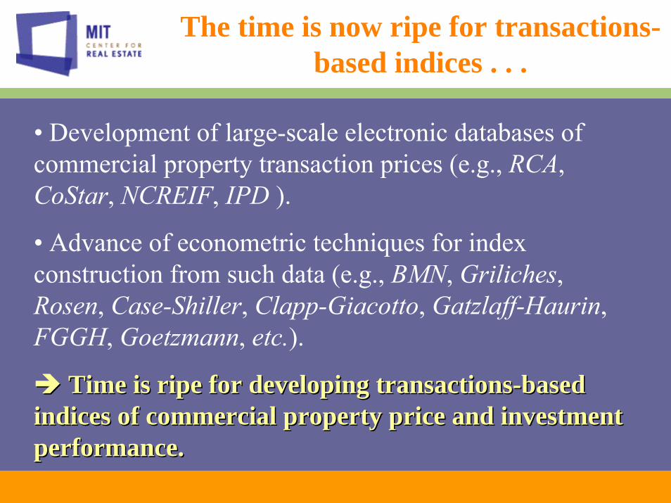
• Development of large-scale electronic databases of commercial property transaction prices (e.g., RCA, CoStar, NCREIF, IPD ).

• Advance of econometric techniques for index construction from such data (e.g., BMN, Griliches, Rosen, Case-Shiller, Clapp-Giacotto, Gatzlaff-Haurin, FGGH, Goetzmann, etc.).

Time is ripe for developing transactionsTime is ripe for developing transactions--based based indices of commercial property price and investment indices of commercial property price and investment performance.performance.

The time is now ripe for transactions-based indices . . .

1. Index return reporting frequency (m = index reporting periods per year);

2. Frequency of revaluation observations per property (f = valuation obs/yr per property);

3. Number of properties in the underlying population tracked by the index (p): Data density = Number of valuation obsper index reporting period = n = pf / m ;

4. Index construction “technology,” or methodology used to construct the index from the underlying valuation observations.

Four Determinants of Index Dynamic Quality:

Exhibit 1a: The General TradeExhibit 1a: The General Trade--off Between Index Statistical Quality Per off Between Index Statistical Quality Per Period, and the Index Reporting FrequencyPeriod, and the Index Reporting Frequency

Increase Return Reporting Frequency m

Incr

ease

Sta

tistic

al Q

ualit

y Pe

r Per

iod

Exhibit 1b: Index Utility Exhibit 1b: Index Utility IsoquantsIsoquants: Index Utility Increases With Both : Index Utility Increases With Both Statistical Quality Per Period and Reporting Frequency: UStatistical Quality Per Period and Reporting Frequency: U00 < U< U11 < U< U22; ; With Diminishing Marginal Substitutability (convex With Diminishing Marginal Substitutability (convex isoquantsisoquants))……


Incr

ease

Sta

tistic

al Q

ualit

y Pe

r Per

iod

U1

U2

U0

Exhibit 1c: Optimal Index Reporting Frequency Is Ambiguous or NoExhibit 1c: Optimal Index Reporting Frequency Is Ambiguous or Not t Unique . . .Unique . . .


Incr

ease

Sta

tistic

al Q

ualit

y Pe

r Per

iod

U1

U2

U0

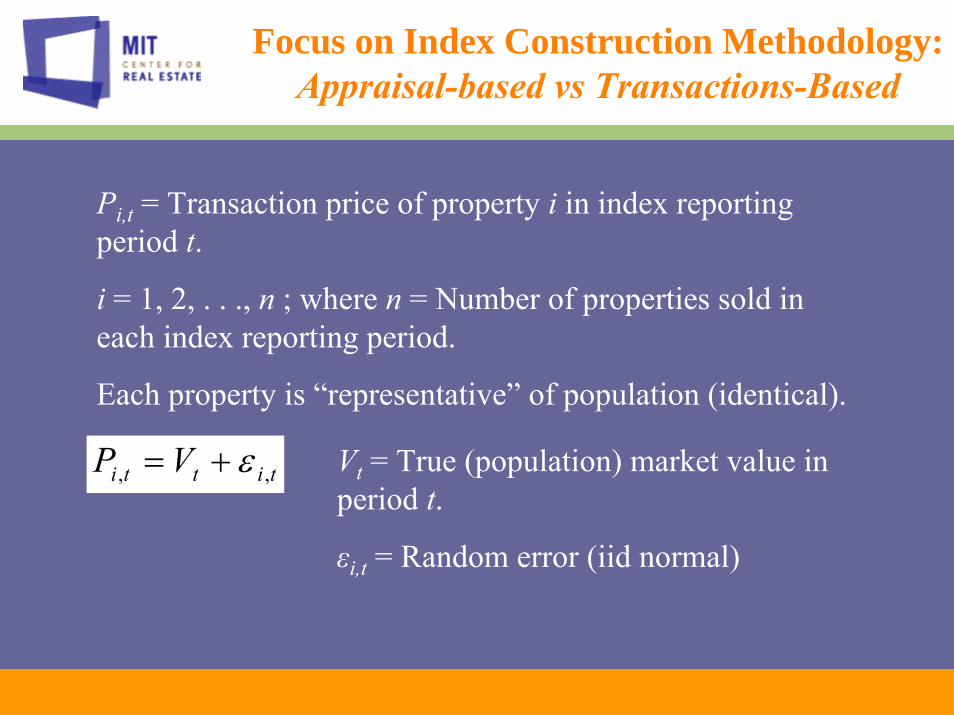
Focus on Index Construction Methodology:Appraisal-based vs Transactions-Based

Pi,t = Transaction price of property i in index reporting period t.

i = 1, 2, . . ., n ; where n = Number of properties sold in each index reporting period.

Each property is “representative” of population (identical).

titti VP ,, ε+= Vt = True (population) market value in period t.

εi,t = Random error (iid normal)

∑=

=N

itiNt PNV

1,

1][ˆ

∑∑=

−

−

=− +==

L

sst

nN

sstt V

LV

nNNVE

0

1

0 111]][ˆ[

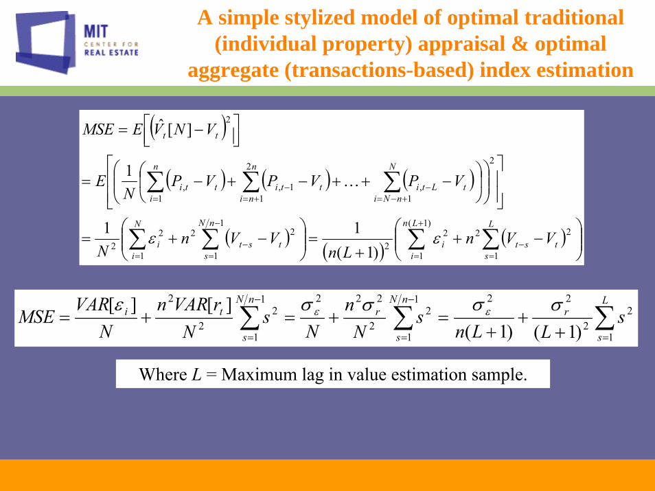
A simple stylized model of optimal traditional (individual property) appraisal & optimal

aggregate (transactions-based) index estimation

= Arithmetic average across N of the transaction prices starting with transactions that are among the n that occur within period t ;

N / n = an integer >= 1.

][ˆ NVt

( )

( ) ( ) ( )

( )( )

( ) ⎟⎟⎠

⎞⎜⎜⎝

⎛−+

+=⎟⎟

⎠

⎞⎜⎜⎝

⎛−+=

⎥⎥⎦

⎤

⎢⎢⎣

⎡⎟⎟⎠

⎞⎜⎜⎝

⎛⎟⎠

⎞⎜⎝

⎛−++−+−=

⎥⎦⎤

⎢⎣⎡ −=

∑ ∑∑ ∑

∑∑∑+

= =−

=

−

=−

+−=−

+=−

=

)1(

1 1

2222

1

1

1

2222

2

1,

2

11,

1,

2

)1(11

1

][ˆ

Ln

i

L

ststi

N

i

nN

ststi

N

nNitLti

n

nitti

n

itti

tt

VVnLn

VVnN

VPVPVPN

E

VNVEMSE

εε

K

∑∑∑=

−

=

−

= ++

+=+=+=

L

s

rnN

s

rnN

s

ti sLLn

sN

nN

sN

rVARnN

VARMSE

1

22

221

1

22

2221

1

22

2

)1()1(][][ σσσσε εε



Where L = Maximum lag in value estimation sample.

221

21

1

2

)2)(1(1

12 εσσ ⎟⎟⎠

⎞⎜⎜⎝

⎛++

−

⎟⎟⎟⎟

⎠

⎞

⎜⎜⎜⎜

⎝

⎛

+−

+=

ΔΔ ∑∑

=

+

=

LLnL

s

L

s

LMSE

r

L

s

L

s

2

21

21

1

2

221

21

1

2

)2)(1(12

,)2)(1(

112

,0

r

L

s

L

s

r

L

s

L

s

nLL

L

s

L

s

LLnL

s

L

s

LMSE

σσ

σσ

ε

ε

=++

⎟⎟⎟⎟

⎠

⎞

⎜⎜⎜⎜

⎝

⎛

+−

+

⇒⎟⎟⎠

⎞⎜⎜⎝

⎛++

=

⎟⎟⎟⎟

⎠

⎞

⎜⎜⎜⎜

⎝

⎛

+−

+

⇒=Δ

Δ

∑∑

∑∑

=

+

=

=

+

=



MSE as a function of lag:

Optimal valuation methodology rule (minimizing MSE):

Optimal lag is:

• Increasing function of the price dispersion σε , and

• Decreasing function of both the transaction density n and the market return volatility σr

• A function only of the ratio of the two dispersion parameters: σε / σr , not of the absolute values of these parameters.



This model is essentially a discrete time version of Quan and Quigley’s (1991) continuous time optimal appraisal model, except that the Quan-Quigley model was conditioned on the existence of a prior value estimate by the same appraiser (optimal updating), whereas the present model is an unconditional optimization, not assuming any prior value estimation.

By working in discrete time, we can address important index policy issues, such as index reporting frequency and transaction price sample size.

Our model here is also very similar to, and our results here are consistent with, those in Giaccotto and Clapp (1992) and Geltner (1997b). Giaccotto & Clapp explored a broader range of appraisal rules and allowed for serial correlation in the market value returns. Geltner (1997b) employed a numerical simulation rather than an analytical model, had declining appraiser weights on comps with the age of the comp, and also relaxed the random walk assumption of the underlying true real estate returns.



Exhibit 2: Optimal Lag (L) as Function of Dispersion Ratio & Transaction Density: (Optimal Lag in Number of Periods)

Dispersion Ratio (σε/σr): Transaction Density: 4 2 1 0.5

n = 1 6 3 1 0 n = 2 4 2 0 0

n = 10 1 0 0 0 n = 35 0 0 0 0



To determine the optimal lag, we employ a numerical algorithm that starts with L = 0, and increments one lag at a time as long as the MSE is decreasing. e.g.:

Optimal lag diminishes rapidly as transaction density increases and as (σε / σr)decreases.

Optimal lag = 0 for transaction densities as low as n = 2 & (σε / σr) as high as 1.

Exhibit 3: RMSE at Optimal Lag (L, & Optimal Sample Size N) as a Function of Transaction Density and Market Volatility (both per period). (Assuming σε = 10%, σr = 10%/year)

Volatility per Period, σr : Transaction Density per

Period:

(Monthly Index) 2.9% = 10% / 12

(Quarterly Index) 5.0% = 10% / 4

(Annual Index) 10.0% = 10% / 1

n = 1 5.42% (L=5, N=6) 6.85% (L=3, N=4) 8.66% (L=1, N=2) n = 3 3.95% (L=3, N=12) 4.79% (L=1, N=6) 5.77% (L=0, N=3)

n = 12 2.50% (L=1, N=24) 2.89% (L=0, N=12) 2.89% (L=0, N=12)



Empirical evidence σε and σr range from 5 percent to 10 percent per year.

Dispersion ratio range between 1/2 and 2 for annual frequency periods, dispersion ratio between 1 and 4 for quarterly periods.

Assuming σε = 10%, we have Exhibit 3…

Exhibit 4a: The Noise Exhibit 4a: The Noise vsvs Lag TradeLag Trade--off Frontier and Optimal Property off Frontier and Optimal Property Value Estimation MethodologyValue Estimation Methodology

Reduced random error

Red

uced

tem

pora

l la

g bi

as

T

U1

A

U2

U0T

LA /2

σε2 /NA

Implications for Appraisal-Based and Transactions-Based Indices:

Exhibit 4b: Greater Utility for an UpExhibit 4b: Greater Utility for an Up--toto--Date Valuation:Date Valuation:


Red

uced

tem

pora

l la

g bi

as

T B

U1

U2

U0

T

LB /2

σε2 /NB

L = Lag of oldest observation in estimation sample for period t.

N = Number of observations in estimation sample for period t.

LB < LA

NB < NA

Implications for Appraisal-Based and Transactions-Based Indices:

Random Error (fraction of σε2 )

Lag

Bia

s in

Perio

ds 0

1

3

U = MIN[RMSE] = 5.09%

Exhibit 5: Optimal Valuation Methodology for Traditional AppraisExhibit 5: Optimal Valuation Methodology for Traditional Appraisal: al: UU = = MINMIN[MSE], [MSE], nn = 1, (= 1, (σσεε / / σσrr) = 4: ) = 4:

LLAA = 6, = 6, NNAA = 7.= 7.EE[[laglag] = 3 periods; ] = 3 periods; Random Error Variance = Random Error Variance = σε2 / 7.RMSE = 5.09% if σε = 10%.

Optimum @ Tangent Pt. “A”.

A

n = Number of available transaction observations per period.

N = Number of transaction observations used in estimation of value as of period t.

L = Maximum lag of transaction observations in estimation sample.

1 1/2 1/7

∑=

⎟⎠⎞

⎜⎝⎛+=

6

1

222

7025.

710.%09.5

ss

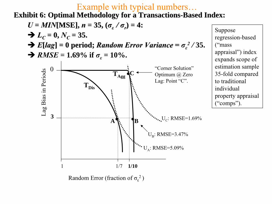
Example with typical numbers…


Lag

Bia

s in

Perio

ds 0

UC: RMSE=1.69%

Exhibit 6: Optimal Methodology for a TransactionsExhibit 6: Optimal Methodology for a Transactions--Based Index: Based Index: UU = = MINMIN[MSE], [MSE], nn = 35, (= 35, (σσεε / / σσrr) = 4: ) = 4:

LLCC = 0, = 0, NNCC = 35.= 35.EE[[laglag] = 0 period; ] = 0 period; Random Error Variance = Random Error Variance = σε2 / 35.RMSE = 1.69% if σε = 10%.

UA: RMSE=5.09%

UB: RMSE=3.47%

“Corner Solution”Optimum @ Zero Lag: Point “C”.

3

TDis

CTAgg

A B

1 1/7 1/10

Suppose regression-based (“mass appraisal”) index expands scope of estimation sample 35-fold compared to traditional individual property appraisal (“comps”).



Lag

Bia

s in

Perio

ds 0

UC: RMSE=1.69%

Exhibit 6: Optimal Methodology for a TransactionsExhibit 6: Optimal Methodology for a Transactions--Based Index: Based Index: UU = = MINMIN[MSE], [MSE], nn = 35, (= 35, (σσεε//σσrr) = 4: ) = 4:

LLCC = 0, = 0, NNCC = 35.= 35.EE[[laglag] = 0 period; ] = 0 period; Random Error Variance = Random Error Variance = σε2 / 35.RMSE = 1.69% if σε = 10%.

UA: RMSE=5.09%

UB: RMSE=3.47%


3

TDis

CTAgg

A B

1 1/7 1/10

B: Index is aggregation of optimal individual appraisals.

C: Index is optimized at aggregate level.



Lag

Bia

s in

Perio

ds 0

UC: RMSE=1.69%

UA: RMSE=5.09%

UB: RMSE=3.47%


3

TDis

CTAgg

A B

Numerical Example Comparison of Appraisal-Based vs Transactions-Based Aggregate Property Value Index. (Error components measured in square root of variance.)

1 1/7 1/10

Error Type: Appraisal-Based Index: Transactions-Based Index: Purely Random (noise): 0.64% 1.69% Temporal Lag Bias: 3.41% 0 Total: 3.47% 1.69%

0341.07

025. 6

1

22

=⎟⎠⎞

⎜⎝⎛ ∑

=ss

3510.00169.0

2

=∑=

⎟⎠⎞

⎜⎝⎛+=

6

1

222

7025.

35*710.0347.0

ss0064.0

35*710. 2

=

TDis

TAgg

Exhibit 7: NoiseExhibit 7: Noise--vsvs--Lag TradeLag Trade--off Frontiers with Disaggregate (Traditional off Frontiers with Disaggregate (Traditional Appraisal) and Aggregate (Transactions Based Regression) ValuatiAppraisal) and Aggregate (Transactions Based Regression) Valuation Methodologieson Methodologies

NNAA = Disaggregate (Appraisal) Optimal Sample Size (# comps) = = Disaggregate (Appraisal) Optimal Sample Size (# comps) = nnAA(L(LAA+1), +1), nnAA = comps density/period= comps density/period; ; NNCC = Aggregate (Transactions Based Regression) Optimal Sample Size = Aggregate (Transactions Based Regression) Optimal Sample Size ((obsobs per period);per period);QQ = Number of Market Segments in the Index Population (as multipl= Number of Market Segments in the Index Population (as multiple of number used by appraiser).e of number used by appraiser).

U0

AU1

Red

uced

tem

pora

l la

g bi

as

B

C0

“Corner Solution”Optimum @ Zero Lag.


TAgg

TDis


LA /2

Lag Bias in Periods

01/(QNA)1/NC1/NA

TDis

TAgg

Exhibit 7: NoiseExhibit 7: Noise--vsvs--Lag TradeLag Trade--off Frontiers with Disaggregate (Traditional off Frontiers with Disaggregate (Traditional Appraisal) and Aggregate (Transactions Based Regression) ValuatiAppraisal) and Aggregate (Transactions Based Regression) Valuation Methodologieson Methodologies

NNAA = Disaggregate (Appraisal) Optimal Sample Size (# comps) = = Disaggregate (Appraisal) Optimal Sample Size (# comps) = nnAA(L(LAA+1), +1), nnAA = comps density/period= comps density/period; ; NNCC = Aggregate (Transactions Based Regression) Optimal Sample Size = Aggregate (Transactions Based Regression) Optimal Sample Size ((obsobs per period);per period);QQ = Number of Market Segments in the Index Population (as multipl= Number of Market Segments in the Index Population (as multiple of number used by appraiser).e of number used by appraiser).

U0

AU1

Red

uced

tem

pora

l la

g bi

as

B

C0

“Corner Solution”Optimum @ Zero Lag.


TAgg

TDis


LA /2

Lag Bias in Periods

01/(QNA)1/NC1/NA

B: Index is aggregation of optimal individual appraisals.

C: Index is optimized at aggregate level.

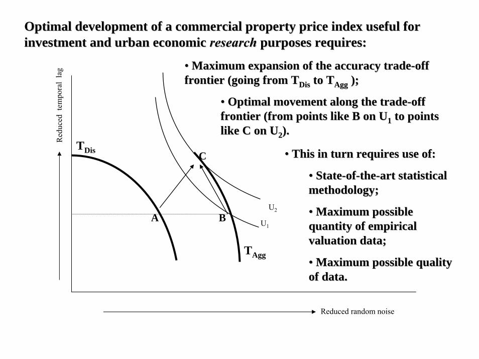
•• Maximum expansion of the accuracy tradeMaximum expansion of the accuracy trade--off off frontier (going from frontier (going from TTDisDis to to TTAggAgg ););

•• Optimal movement along the tradeOptimal movement along the trade--off off frontier (from points like B on Ufrontier (from points like B on U11 to points to points like C on Ulike C on U22). ).

Optimal development of a commercial property price index useful Optimal development of a commercial property price index useful for for investment and urban economic investment and urban economic researchresearch purposes requires:purposes requires:

•• This in turn requires use of:This in turn requires use of:

•• StateState--ofof--thethe--art statistical art statistical methodology;methodology;

•• Maximum possible Maximum possible quantity of empirical quantity of empirical valuation data;valuation data;

•• Maximum possible quality Maximum possible quality of data.of data.

Reduced random noise

Red

uced

tem

pora

l la

g

TDis

TAgg

U2

C

U1BA

• For research that is highly sensitive to temporal lag bias, but less sensitive to random error in the index returns, transactions-based indices are preferableto appraisal-based indices, because of the temporal lag bias inherent in appraisal-based returns.

Implications of the Model (1):

• For research that is highly sensitive to random error, but not very sensitive to temporal lag bias, an appraisal-based index may be preferable to a transactions-based index because of the greater frequency of the appraisals in the population and (possibly) because the appraisals may be less noisy than the transaction prices.


• For research that is equally sensitive to lag bias error and random error (e.g., as represented by the MSE-minimization objective for the index), transactions-based indices are preferable to appraisal-based indices.


• Except for indices tracking small populations of properties where transaction density is less than two or three dozen observations per index reporting period, transactions-based indices minimizing the MSE criterion can be produced with no temporal lag bias.


Considerations in the Design & Construction of … 17, 2000 · Considerations in the Design &...

Documents

Transcript of Considerations in the Design & Construction of … 17, 2000 · Considerations in the Design &...