Conservation of Endangered Species: Can Incentives Work

for Private Landowners?

Christian Langpap

Dept. of Agricultural and Resource Economics, Oregon State University, Corvallis, OR 97331.

Ph.: (541) 737 1446, Fax: (541) 737 2563 E-mail: langpapc@onid.orst.edu.

Paper prepared for presentation at the American Agricultural Economics Association Annual Meeting,

Montreal, Canada, July 27-30, 2003

Copyright 2003 by Christian Langpap. All rights reserved. Readers may make verbatim copies of this

document for non-commercial purposes by any means, provided that this copyright notice appears on all such

copies.

Conservation of Endangered Species: Can Incentives Work

for Private Landowners?

Abstract

It has been argued that the traditional regulatory approach of the Endangered Species Act,

based on land-use restrictions, has failed to protect endangered species on private land. In

response, there has been a call for the use of incentives to complement this regulatory

approach. This paper examines the potential of incentives programs to elicit conservation-

oriented management choices from landowners. Data obtained from a survey of non-

industrial private forest owners in Oregon and Washington is used to examine the

effectiveness of various incentives. The results indicate that incentives, in particular

compensation and assurances, can be effective in increasing the conservation effort

provided by landowners. The results also suggest that conservation policy for private lands

could be improved by relying on a combination of incentives, including financial incentives

and assurances, rather than exclusively on the threat of regulation.

1

Conservation of Endangered Species: Can Incentives Work for Private

Landowners?

INTRODUCTION

The conservation of endangered species on private land remains a controversial

topic. Section 9 of the Endangered Species Act (ESA) prohibits any private action that may

directly result in the taking of endangered species. Additionally, as interpreted by the U.S.

Fish and Wildlife Service (FWS), it restricts any activity that may indirectly harm a species

by modifying its habitat in ways that hinder essential activities, such as feeding and

breeding1. These restrictions can encompass otherwise lawful activities such as logging,

construction, or grazing, and thus have raised vigorous opposition from property rights

advocates. As a result, enforcement of Section 9 has become increasingly difficult. This

could severely undermine endangered species recovery efforts under the ESA, because

more than half of the listed endangered species have at least 80% of their habitat on private

land (FWS 1997a).

Furthermore, it has been widely maintained that a common reaction by landowners

to the prospect of these restrictions is to “shoot, shovel, and shut up”. That is, the traditional

approach to regulation may generate perverse incentives that compel landowners to manage

their land in ways that discourage the presence of endangered species, in order to avoid

land-use restrictions. This argument has been made formally by Polasky and Doremus

(1998), Innes (2000), and Polasky (2001), and anecdotal evidence of such behavior

abounds (see, e.g., Mann and Plummer 1995, Bean and Wilcove 1997, Bean 1998).

1 This interpretation was upheld by the Supreme Court in Babbitt v. Sweet Home Chapter of Communities for a Great Oregon, 515 U.S. 687 (1995).

2

Michael and Lueck (2000) have found empirical evidence of this behavior in the case of

private forest owners in the southeast and the red-cockaded woodpecker.

Another potential drawback of Section 9 of the ESA is that it is “all sticks and no

carrots”, since its goal is to prevent harmful conduct by landowners rather than encourage

desirable behavior. For many endangered species, benign neglect might be insufficient to

bring about recovery, as they require active management of their habitat (Bean and Wilcove

1996, Bean 1998). This can give rise to costs that even well-meaning landowners might not

be willing to undertake. Additionally, there are opportunity costs of forgone revenue from

the most profitable use of the property.

Thus, Section 9 of the ESA seems to grant inadequate protection to endangered

species on private land, and may even cause the very behavior it attempts to prevent.

Hence, there has been a call for the use of incentives-based voluntary programs to

complement the existing regulatory framework. Two main approaches have been

suggested. The first one is based on agreements that provide landowners with assurances

regarding future regulation, such as “no surprises” Habitat Conservation Plans or Safe

Harbor Agreements (Wilcove et al. 1996, Bean and Wilcove 1996). The second approach is

based on offering the landowner incentives to manage his land in a way that is compatible

with the survival and recovery of endangered species. These incentives include, for

example, compensation payments, tax credits, cost sharing agreements, public recognition,

and stewardship certification (see, e.g., Keystone Center 1995 or Vickerman 1998).

Much of the existing literature on incentives for conservation has focused on their

application on farmland. For instance, McLean-Meyinsse et al. (1994) examine small

farmers’ willingness to participate in the Conservation Reserve Program (CRP), and

Cooper and Osborn (1998) analyze re-enrollment in the CRP as a function of the rental rate

3

paid. Smith (1995) uses mechanism design theory to characterize the properties of a least-

cost CRP, and Wu and Babcock (1996) derive optimal payment schedules for an

environmental stewardship program.

The use of incentives has been examined in the case of private forest owners as

well. Boyd (1984) evaluates the impact of cost-sharing and forester assistance on non-

industrial timber supply. Royer (1987) shows that the reforestation decisions of landowners

are responsive to cost-sharing assistance. Hardie and Parks (1996) analyze how cost sharing

could have affected investment in pine regeneration between 1971 and 1981. Kluender et

al. (1999) find that landowners who manage their forest for timber would engage in

forestry practices regardless of assistance payments.

There is also a growing literature that specifically addresses the use of incentives to

promote management that benefits endangered species (see, e.g., Smith and Shogren 2001,

2002, Defenders of Wildlife 1994, Stone 1995, Kennedy et al. 1996, Bourland and Stroup

1996). However, there have been relatively few formal empirical analyses of the effect of

incentives on private landowners’ decisions. Kline et al. (2000) examine the willingness of

non-industrial private forest owners (NIPFs) to forego harvesting to improve habitat for

endangered salmon. Zhang and Flick (2001) measure the impact of both the ESA and cost-

share and tax incentives on the reforestation investment behavior of NIPFs.

This paper adds to this literature by analyzing the likely effects of assurances, cost

sharing, and compensation incentives on landowners’ management decisions in the specific

context of endangered species conservation. I used data from a survey of NIPFs in Oregon

and Washington to construct econometric models that measure the probable effect of these

incentives on landowners’ willingness to provide conservation effort. This allowed me to

assess the potential of these incentives as a policy tool for managing endangered species on

4

private land. Additionally, the estimates from the econometric models were used to

examine the effectiveness of different incentive program designs.

The results obtained provide evidence that conservation policy for protecting

endangered species on private land could be improved by offering “carrots” to landowners

to complement the existing regulatory “sticks”. Specifically, the analysis indicates that

compensation and assurances could have a significant effect on landowner’s management

decisions, but cost sharing may not. Furthermore, the results suggest that policy makers can

design more effective incentives programs by combining financial incentives with

assurances about future regulation.

The remainder of this paper is organized as follows. First, I present an analytical

framework to motivate the econometric analysis, followed by a description of the data and

the survey instrument used to obtain it. After that, I present the econometric model and the

empirical results. Then, a simulation is conducted to analyze the implications of the

empirical results for the design of incentives programs. Finally, I discuss the main findings

and conclude.

ANALYTICAL FRAMEWORK

In this section, I assume that a landowner has voluntarily agreed to participate in a

conservation agreement, and I use a simple model to examine how different incentives can

affect the amount of conservation effort the landowner is willing to supply. This analysis

will provide a basis for the development of the survey instrument and the empirical models

that follow.

Following Langpap and Wu (2002), I use a two period model of the interaction

between a landowner and a regulator, in which the first period represents the present and

the second period represents the entire future time horizon. Suppose that at the beginning of

5

period 1 a regulator, such as the FWS, approaches a landowner and proposes that he

voluntarily participate in a conservation agreement and supply conservation effort levels cv1

and cv2 for periods 1 and 2, respectively. To fix ideas, suppose that cv1 and cv2 represent a

specific management plan for the property.

At the beginning of period 2 the regulator may learn that a change in the

management plan is necessary (for instance, new knowledge about a species may become

available, or an unforeseeable event may alter the status of a species), and thus he may

require that the management plan for period 2 be *2c > cv2. This occurs with probability q.2

Although the required changes are not known until the second period, in period 1 the

landowner forms an expectation about the alternative management plan, denoted by E *2c .

In exchange for participating and supplying conservation effort, the landowner is

offered one or more of three incentives: cost sharing on out-of-pocket costs of

implementing the management plan, assurances that no additional conservation effort will

be required in period 2 (i.e. that the management plan in period 2 will be cv2, as originally

agreed, rather than *2c ), and compensation for opportunity costs of implementing the

management plan.

The landowner may reject the proposition. If he does, he faces the possibility that,

with probability p, the regulator will impose mandatory conservation levels *1mc and E *

2mc ,

which could represent restrictions on harvesting or development on the property3. If no

2 The probability q characterizes the regulator’s a priori unknown willingness or ability to require more conservation. For instance, the regulator may be unwilling or unable to modify an existing management plan for political reasons or due to lack of funding for additional research and enforcement expenses. 3 Regulation is uncertain because the regulator may be unable or unwilling to enforce the law due to information requirements, high burden of proof, or political considerations (Polasky and Doremus 1998).

6

mandatory conservation is imposed, the landowner develops his property, and thus does not

supply any conservation effort.

Let ai and bi be the unit out-of-pocket and opportunity costs of conservation,

respectively, for i = v, m. Out-of-pocket costs include, for example, labor and machinery

costs of thinning a stand of forest. Opportunity costs include, for example, the revenue

forgone when a stand of forest is not harvested. Additionally, let γ be the fraction of out-of-

pocket costs incurred by the landowner under a cost-sharing incentive. Similarly, let α be

the portion of opportunity costs incurred by the landowner under a compensation incentive.

I assume that the costs of conservation are linear, and that it is cheaper to provide a given

conservation effort under a voluntary agreement than under a mandatory agreement, i.e. av

+ bv < am + bm. The reasoning behind this assumption is that a voluntary agreement

provides more flexibility for the landowner to choose the most cost-effective way to

provide any given level of conservation effort. The landowner will accept the regulator’s

proposition and implement management plan (cv1, cv2) if and only if

(γav+αbv)cv1+q(γav+αbv)E *2c +(1 – q)(γav+αbv)cv2 ≤ p(am+bm)( *

1mc + E *2mc ) (1)

The cost sharing, compensation, and assurances incentives are thus given by γ < 1, α < 1,

and q = 0, respectively. Decision rule (1) can be rearranged to define the landowner’s

acceptance set

SL = {(cv1, cv2)|cv1 + (1- q)cv2 ≤ p vv

mm

babaαγ +

+ ( *1mc + E *

2mc ) – qE *2c } (2)

This set can be interpreted as containing all the management plans that the landowner will

accept as part of a conservation agreement. The set SL is shown in Figure 1.

7

Suppose that the regulator and the landowner reach an agreement, under which the

landowner will provide the maximum conservation effort he is willing to supply4. That is,

condition (1) holds with equality. This means that the management plan (cv1, cv2) is on the

upper boundary of the set SL in Figure 1. If this management plan does not coincide with

the regulator’s first choice of conservation effort (for instance, that which maximizes net

social benefits from conservation, as in Langpap and Wu 2002), the regulator may try to

elicit higher conservation effort by using cost sharing, compensation, and assurances

incentives. To understand the potential effect of these incentives, I examine how changes in

the incentive parameters γ, α, and q affect decision rule (1) and the acceptance set SL.

Starting from a base scenario in which no incentives are offered, i.e. γ = α = 1 and q > 0, the

regulator can increase the level of conservation effort by setting γ' < 1 and α' < 1 and by

offering assurances, which sets q = 0. Thus, decision rule (1) becomes

(γ'av + α'bv)cv1 + (γ'av + α'bv)cv2 ≤ p(am + bm)( *1mc + E *

2mc ) (3)

and the acceptance set is

SL' = {(cv1, cv2)|cv1 + cv2 ≤ p vv

mm

baba

'' αγ ++ ( *

1mc + E *2mc )} (4)

By comparing conditions (1) and (3), and sets (2) and (4), it is clear that cost sharing and

compensation (γ' < γ, α' < α) can increase the conservation effort provided by the landowner

by decreasing the cost of conservation. Additionally, Langpap and Wu (2002) show that

offering assurances can increase the conservation effort supplied by the landowner when

additional conservation is expected in the second period. The effect of these incentives is

shown in Figure 2. The management plan with cost sharing, compensation, and assurances

4 Langpap and Wu (2002) discuss the necessary and sufficient conditions for such an agreement. The landowner participates because of the cost advantage offered by voluntary agreements (as long as the expected future conservation requirements are not too large).

8

incentives is on the upper boundary of the set SL' (the solid line), which is above that of the

set SL (the dashed line), corresponding to the case of no incentives. This indicates that a

higher level of conservation effort is supplied when incentives are offered.

There are other factors, not considered explicitly in this simple model, which can

affect the landowner’s response to these incentives. For instance, the availability of

technical assistance may lower the cost of conservation for some landowners. The

opportunity cost of conservation may depend on characteristics of the landowner’s

property, such as size, or, in the case of a forest, the age of the trees. Additionally,

landowners may derive utility from conservation, which could affect the opportunity cost.

This utility, and therefore the opportunity cost, can depend on the landowner’s original

management plan for the property, as well as demographic characteristics such as age,

occupation, or income. Furthermore, the landowner’s perceived threat of regulation can

affect the parameter p in the model, and thereby have an effect on the response to the

incentives. Finally, other factors, such as the availability of technical assistance, could

affect the cost of conservation as well.

In the following sections, I examine empirically whether cost sharing,

compensation, and assurances can have an effect on the management plan that a landowner

is willing to implement, as the results from this simple model suggest. The role played by

other factors, such as landowner and property characteristics, will be analyzed as well.

SURVEY AND DATA

Survey

A survey instrument was designed to examine how landowners’ management

decisions would respond to cost sharing, compensation, and assurances incentives. The

study area included 25 counties in western Oregon and Washington. The names and

9

addresses of all NIPFs who owned at least 10 acres of land zoned as forest5 were obtained

from county tax assessor offices. A mail survey was designed and conducted according to

the Total Design Method (Dillman 1978) in the summer and fall of 2001. A first version of

the survey was pre-tested with two focus groups of NIPFs. A second version of the survey

was mailed out to a subset of the sample as a further pretest. The final version of the survey

was mailed out to 1,500 NIPFs, followed by a reminder postcard, and second and third

mailings to non-respondents. Of the original 1,500 mailings, 101 surveys were

undeliverable, so the final sample consisted of 1,399 forest owners. Seven hundred and

thirty seven of the returned surveys were usable, which yields a response rate of 53% (or

49% of the entire sample of 1,500). Finally, a sample of 137 non-respondents (30% of total

non-responses) were contacted by phone and asked for information on characteristics that

could influence response6. This information was used to conduct a test for sample-selection

bias, which is described below.

As in the analytical model, survey recipients were asked if they would be willing to

participate in a conservation agreement, and presented with a choice of three hypothetical

“incentives programs”. Respondents who answered that they would not be willing to

participate, regardless of the incentives offered, were excluded from the sample. Each

program contained a management plan and some combination of the various incentives, as

well as a technical assistance attribute. Landowners also had the option not to accept any of

the incentives programs offered (see the Appendix for an example). This choice was

5 Ten acres was chosen as a cutoff point because the distribution of landowners showed that there are relatively large numbers of landowners with small properties (up to 10 acres) and comparatively few owners with larger properties. Thus, a random sample that included all acreages would have resulted in larger landowners, who own most of the acreage, being underrepresented. Additionally, smaller holdings are more likely to be held as rural-residential properties, and not as forestland. 6 Specifically, I obtained information on importance given to services provided by the landowner’s forest, total acres owned, years they have owned the property, knowledge of incentives programs, perceived likelihood of regulation, age, occupation, and income.

10

presented three times to each survey recipient, and the composition of the incentives

programs was varied across different versions of the survey. This setup makes it possible to

observe how the landowners’ willingness to implement different management plans varies

as the levels of the various incentives change, and thus to measure the effect of these

incentives on the level of conservation effort supplied. Additionally, to take into account

other factors that may influence the landowner’s response to the incentives, the survey

included questions on characteristics of their land, their perceived risk of regulation under

the ESA, and demographic information.

Data

The three management plans presented to landowners in the survey consisted of one

or more of three silvicultural techniques: thinning, providing snags and downed logs, and

managing under story vegetation. Implementation of these techniques may speed the

development of forest structures required by endangered species commonly associated with

the Pacific Northwest, such as spotted owl, marbled murrelet, and salmon (FWS 1992,

1997b, USDA 1993, Hayes et al. 1997). Plan 1 consists only of thinning, Plan 2 includes

thinning and providing snags and logs, and Plan 3 consists of thinning, providing snags and

logs, and managing under story vegetation. A key feature of these management plans is that

they are progressively more complex, and hence increasingly beneficial to the species and

costly to the landowner as well. These management plans are a proxy for the landowner’s

readiness to supply conservation effort. The increasing complexity provides a sense of

ordering that makes it possible to measure whether incentives can elicit higher conservation

effort. The resulting measure is the dependent variable in the model, PLAN = 0, 1, 2, or 3,

where PLAN = 0 represents no conservation effort.

11

The main independent variables (SHARE, COMP, ASSURE) measure the levels of

cost sharing, compensation, and assurances incentives offered. To account for the

possibility that the effectiveness of these incentives may vary with income levels,

opportunity costs, and the perceived probability of regulation, the incentive regressors were

allowed to interact with these variables. Additionally, a landowner’s choice of management

plan may depend on the availability of technical assistance. Thus, the model includes a

variable that indicates whether assistance is available or not (ASSIST).

The survey asked landowners how likely they believed it was that the ESA might

restrict timber harvesting, development, or other activities on their land. The variable

REGULATE is the likelihood of regulation given by the landowner on a 5-point scale,

ranging from “Very Unlikely” to “Very Likely”. The model also includes a number of

demographic and land-characteristic variables that may have an effect on the cost of

conservation. Finally, landowners were asked to consider a specific stand on their property

where they might be willing to implement a management plan, and to provide information

about this stand. The size and age of this stand (STANDSIZE, STANDAGE) are included

to control for opportunity costs of participating in the incentives program. In addition, I

control for alternative uses of the stand by including two dummy variables that describe the

landowner’s harvesting plans. A description of all these variables, along with summary

statistics, is presented in Table 17.

7 Earlier versions of the model explored the role of variables measuring the importance given by the landowner to various services provided by his forest, variables describing the landowner’s knowledge of and experience with incentives programs, and variables controlling for membership in forestry and conservation organizations. None of these had a significant effect on management decisions, so they were left out of the models presented here.

12

ECONOMETRIC MODELS AND RESULTS

Given the ordered nature of the dependent variable, the model used for estimation is

an ordered probit. Likelihood ratio tests revealed that some of the regressors (SHARE,

ASSURE, ASSIST, SHXIN, ASXRE, STANDSIZ, HARV40) were heteroscedastic. To

accommodate this, I used a general multiplicative formulation for the variance of the

disturbances (Greene 2000): Var[ε] = [exp(ν'z)]2, where z is the vector of heteroscedastic

variables. With this specification, the log-likelihood function for the model is

ln L= ∑=0PLAN

ln Φ(-β'x/eν'z) + ∑=1PLAN

ln[Φ((µ1 - β'x)/eν'z)-Φ(-β'x/eν'z)] +

∑=2PLAN

ln[Φ((µ2 - β'x)/eν'z) -Φ((µ1 - β'x)/eν'z)] + ∑=3PLAN

ln[1-Φ((µ2 - β'x)/eν'z)] (5)

where xi is a vector containing the regressors described in the preceding section (incentives,

landowner and property characteristics), µ1 and µ2 are threshold parameters to be estimated

along with β, and Φ(•) is the cumulative density function for the standard normal

distribution. Table 2 shows the maximum likelihood estimates for two versions of this

model (corrected for heteroscedasticity).

In model 1, the null hypothesis that the parameter estimates for age, education,

occupation, and the variables for property characteristics are all equal to zero could not be

rejected (the p-value for the Wald test is 0.91), so these variables are left out of model 2.

The income dummies are not significant independently, but the null hypothesis that they are

jointly equal to zero can be rejected (p = 0.096). The chi-squared statistics for overall fit

and the scaled R2 statistics indicate that the models have good explanatory power.

Sample Selection Bias

Models 1 and 2 were also tested for potential sample selection bias induced by

survey non-response, a common problem with mail-administered surveys (Mitchell and

13

Carson 1989, Messonier et al. 2000). If non-response occurs in such a way that the factors

that determine a landowner’s choice of management plan and those that determine response

are correlated, then the parameters estimated in the preceding models may be biased. The

information obtained in the follow-up phone survey of non-respondents was used to

conduct a two-step Heckman test for sample selection bias (Heckman 1979, Edwards and

Anderson 1987, Mesonnier et al. 2000). The first step consists of a probit model of

participation in the survey. The resulting parameter estimates are used to calculate the

inverse Mills ratio (λ1), which represents the probability of a recipient having responded

(i.e. being in the sample). The inverse Mills ratio is then included as an additional regressor

in Models 1 and 2 in the second part of the procedure. The test for sample selection bias is

based on a t-test of the significance of the parameter estimate for λ1. If it is not statistically

significant, then the null hypothesis of no sample selection bias cannot be rejected. The

results of this test for models 1 and 2 show that there is no evidence of sample selection

bias: the t-statistics for λ1 are -0.43, and –0.24, respectively.

An additional selection bias test is necessary because those survey respondents who

answered that they would not participate in a conservation agreement regardless of the

incentives offered were excluded from the sample. The two-step Heckman test is repeated,

using a probit model of participation in the conservation agreement based on demographic

and property characteristics of survey respondents. Once again, the results of the test show

no evidence of selection bias: the t-statistics for λ2 (the second inverse Mills ratio) are 0.28,

and – 0.42 for models 1 and 2, respectively.

Results

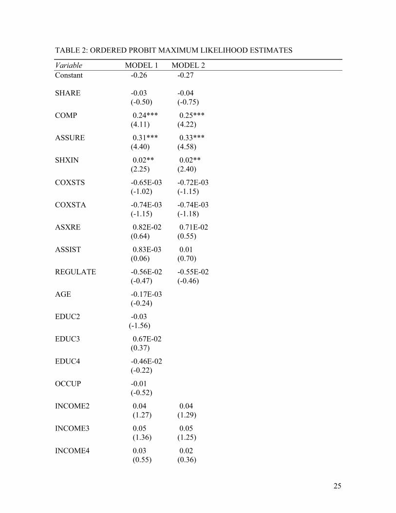
The results presented in Table 2, which are consistent across both models (and

others which are not reported), show that the coefficients of COMP and ASSURE are

14

significantly different from zero, suggesting that compensation and assurances incentives

would have an effect on the probability that landowners supply conservation effort. The

coefficient of SHARE is not significantly different from zero, but that of the interaction

variable for cost sharing and income (SHXIN) is. This suggests that the effect of cost

sharing depends on the level of income. Additionally, the coefficient of HARV40 is

significant, suggesting that landowners who plan to harvest in 40 or more years are more

likely to manage the stand for endangered species than those who have medium- or short-

term harvesting plans. It is also interesting to note that the coefficients of ASSIST and

REGULATE are not significant, suggesting that technical assistance and the perceived

likelihood of regulation may not affect the landowners’ management decisions. These

results are discussed further in section VI.

To understand the effects of the significant incentive variables (COMP and

ASSURE) on the dependent variable, marginal effects were computed as follows. For a

discrete variable that appears in x and z, say xk, define xks and xkf as the starting and final

values of xk, respectively. Additionally, define kx− as the vector of all regressors, except xk,

evaluated at their sample mean. Similarly, define kz− as the vector of heteroscedastic

variables, except xk, evaluated at their sample mean. Then

Pr(PLAN = i|xkj) = Ф[(µi-βkxkj – β-k' kx− )/exp(νkxkj + ν-k' kz− )] – Ф[(µi-1- βkxkj – β-k' kx− )/exp(νkxkj+ν-k' kz− )], j = s, f. The marginal effect of xk is ∆Pr(PLAN = i) = Pr(PLAN = i|xkf) - Pr(PLAN = i|xks)

for i = 0, 1, 2, 3 (Long 1997). Table 3 gives the signs of these marginal effects, and Figure

3 shows the probabilities in that each plan is chosen for the different values of the

compensation and assurances incentives. The marginal effects for the compensation and

15

assurances incentives suggest that increasing the level of compensation and providing

assurances decrease the probability of no effort and a small amount of effort (PLAN=0 and

PLAN =1) and increase the probability of higher levels of conservation effort (PLAN = 2

and PLAN = 3).

These results indicate that incentives could be used effectively to increase the level

of conservation effort supplied by private landowners. They also suggest that some

incentives may be more effective than others. For instance, in the particular scenario

examined here, compensation and assurances would have a more significant effect than

cost sharing. This raises the question of how to optimally design incentives programs by

combining different incentives to achieve the largest effect on landowners’ management

decisions.

DESIGN OF INCENTIVES PROGRAMS

The parameters and marginal effects estimated in the preceding section are based on

the incentives programs presented to landowners in the survey, which included different

combinations of cost sharing, compensation, and assurances incentives. Designing

conservation policy based on incentives may involve having to choose only one type of

incentive (for instance, Habitat Conservation Plans, which provide assurances to

landowners, generally do not offer financial incentives as well), or finding the most

effective mix of incentives. Thus, it is useful to examine how a representative landowner’s

willingness to provide conservation effort changes for different combinations of incentives.

I conduct a simulation of the probabilities that each plan is implemented given

different combinations of incentives, keeping all the other variables constant at their sample

mean. To show the effects of the different incentives clearly, I assume they are applied at

the highest possible level (75% for cost sharing and 100% for compensation). Additionally,

16

I assume that no technical assistance is offered (there is no qualitative change in the results

if assistance is included).

Table 4 shows the simulated probabilities that each plan is chosen. The base

scenario is one in which no incentives are offered. In this case, it is most likely that the

landowner would supply no conservation effort or low effort: the probabilities that he

would choose Plan 0 or Plan 1 add to 99%, whereas the probability of high conservation

effort (Plan 3) is zero. In scenario 1, only cost sharing is offered. This has the effect of

decreasing the probability of no conservation effort (Plan 0) and increasing that of medium

or high levels of effort (Plans 2 and 3). However, the probability that no effort or low effort

is supplied remains high (the probabilities of Plan 0 and Plan 1 add to 77%). Scenario 2

offers only compensation. Relative to the base scenario, the probability of no effort (Plan 0)

decreases considerably, whereas the probability that low or medium conservation effort is

forthcoming (Plans 1 and 2) increases. The probability of high effort (Plan 3) increases

modestly, but remains small. In scenario 3, the landowner receives only assurances. The

probability of no conservation effort (Plan 0) decreases to zero, whereas the probability of

low or medium conservation effort is high (the probabilities of Plan 1 and Plan 2 add to

98%). The probability of high conservation effort (Plan 3) increases slightly relative to the

base scenario, but remains small.

These scenarios suggest that, although all three types of incentives can have an

effect on landowners’ decisions, cost sharing provides the weakest incentive, compensation

has a somewhat stronger effect, and assurances is the most effective incentive. However,

neither of these incentives, when used alone, is sufficient to significantly increase the

probability that a high level of conservation effort (Plan 3) is provided.

17

In scenarios 4 and 5 the financial incentives, cost sharing and compensation, are

combined with assurances. In Scenario 4, a combination of cost sharing and assurances

decreases the probability of no conservation effort (Plan 0) and increases the probability of

low and medium effort (Plans 1 and 2) considerably more than the cost sharing incentive

alone. Finally, in Scenario 5 a combination of compensation and assurances is offered. This

combination would be the most effective in eliciting conservation effort, as the probability

of Plan 3 (high effort) increases to 100%.

These results suggest that the effectiveness of financial incentives can be increased

by combining them with assurances. Adding assurances may increase the marginal effect of

these incentives, making additional amounts of cost sharing or compensation payments

more effective than they would be on their own. This can be seen in Figure 4, which shows

the effects of increasing levels of compensation on the probabilities that each plan is

implemented. In Figure 4a compensation is offered on its own, while in Figure 4b it is

combined with assurances. Although in Figure 4a the probability of Plan 0 decreases as

compensation increases, Plan 0 remains the most likely alternative up to a compensation

level of 70%. It would take full compensation (100%) for a representative landowner to

implement Plan 1. The effect on the probabilities of Plan 2 or Plan 3 being implemented is

small. Figure 4b shows that increasing the level of compensation is considerably more

effective when assurances are offered as well. Plan 3 is the most likely alternative at all

levels of compensation, so compensation of 40% would be sufficient to elicit the highest

level of conservation effort.

This analysis has focused on examining the effectiveness of various combinations

of incentives in eliciting conservation effort from private landowners. Another important

issue, which lies outside the scope of this paper, is the efficiency of the different incentive

18

options from a social perspective. The various incentives may have different implications

for social welfare, which are not addressed in the models presented here. For instance,

funding compensation or cost sharing payments, conceivably through taxation, can generate

a deadweight loss due to administrative costs and to distortions that could make these

incentives less attractive. Providing assurances may also generate opportunity costs to

society if the flexibility to correct management plans when conditions change in the future

is curtailed. Thus, the most effective combinations of incentives, as evaluated here, may not

necessarily be the most socially efficient.

DISCUSSION

The results presented in the preceding sections suggest that the incentives examined

in this paper could be effective in encouraging landowners to manage their property in a

way that is beneficial to endangered species. Specifically, offering compensation and

assurances incentives could increase the likelihood that landowners supply higher levels of

conservation effort. On the other hand, cost sharing may not be as effective in eliciting

conservation effort from landowners. One possible explanation for this result is that the

landowners’ strong feelings about property rights, government intervention, and perceived

unfairness of land use regulation may make compensation and assurances more relevant to

them. Additionally, out-of-pocket costs may be small relative to the lost income and the

perceived future impacts of regulation.

The coefficient for ASSIST is not statistically different from zero either. This

indicates that offering technical assistance may not be effective in inducing landowners to

supply higher levels of conservation effort. One possible explanation for this is that the

landowners may be knowledgeable enough about managing their property to consider

assistance unnecessary. On average, landowners rated the availability of technical

19

assistance as only “somewhat important” in determining their management decisions.

Additionally, comments made by landowners in the survey suggest some animosity towards

the government and foresters or extension agents, often citing negative experiences in the

past8. Thus, landowners may want to keep the government out of their land, and may

distrust foresters or extension agents.

The coefficient for the perceived likelihood of regulation (REGULATE) is not

significant, implying that the “stick” of regulation may not be as effective as the incentive

“carrots” in eliciting conservation effort from landowners. This may be because landowners

do not seem to feel greatly threatened by the ESA: on average, they ranked the likelihood

of regulation between “unlikely” and “even chance”, and 60% of them feel that there is no

more than an even chance that the ESA will restrict activity on their property. Furthermore,

landowners may view other regulations at the state or local level, such as the Oregon Plan

for salmon or Washington’s Forest and Fish rules, as more immediate regulatory threats.

This may explain why the results show that assurances are important to landowners,

although they don’t consider ESA regulation likely.

Finally, the results of the simulation suggest that, although incentives like

compensation and assurances may work on their own, a combination of incentives may be

more effective in compelling landowners to manage their property for endangered species.

In particular, better results can be achieved by combining financial incentives with

assurances. In this specific case, the most effective combination would include

compensation and assurances, since landowners would not be as responsive to the cost

sharing incentive. Many landowners may not be opposed to providing habitat on their land,

8 For instance, landowners commented that they “want no part of any government agency because they lie, cheat, steal”, that there is “too much government in land now; they do a terrible job”, and that “the managing of private land should be left entirely to the landowner”.

20

but hesitate to do so because they fear government intervention or question the fairness of

having to assume the costs of providing a public good. The combination of compensation

and assurances may be the most effective because it addresses these concerns by lowering

the opportunity cost of managing for endangered species, and allowing landowners to keep

control over land management decisions.

These results have interesting implications for conservation policy and the design of

incentives programs. They suggest that the threat of regulation may not suffice to compel

landowners to manage their property in a way that is beneficial to endangered species, in

particular when landowners do not perceive that the threat of regulation is high. On the

other hand, the use of incentives could be highly effective. Specifically, compensation for

lost income and assurances about future regulation can play a significant role in eliciting

conservation effort. Furthermore, combining financial incentives with assurances could

have a larger positive effect on landowners than using either type of incentive on its own.

Thus, conservation policy on private land might be improved by relying on a combination

of incentives, including financial incentives and assurances, rather than exclusively on the

threat of regulation.

An alternative option, of course, would be to make the threat of regulation more real

by bolstering enforcement. This would conceivably increase the importance of assurances

as an incentive. Landowners may not be willing to enter into agreements that include

financial incentives but no assurances, since managing for endangered species given

heightened enforcement would increase the risk of facing land use restrictions. On the other

hand, an increased threat of regulation may make landowners more willing to enter into

incentives programs that do include assurances. Thus, waving a heavier regulatory stick

21

could be effective in encouraging landowners to manage for endangered species as long as

the carrot of assurances is offered as well.

This paper is a first step in evaluating the likely effectiveness of incentives

programs. The framework used here could be applied to other incentives, such as tax

breaks, different types of land, like wetlands or farmland, and different regions. This would

further improve our understanding of the usefulness of these programs.

APPENDIX

16 . Suppose that you a re p resen ted w ith on ly th e following choice. Com pare th e four op tions an d consider wh ich one you would be m ost likely to choose.

Option 1 Option 2 Option 3 Option 4 - Th in n ing to 50 -75

trees/acre, - 2 -4 snags and logs/acre, - M an age under story

(Activities 1 ,2 ,3 )

- Th in n ing to 50 -75 trees/acre, - 2 -4 snags and logs/acre

(Activities 1 ,2 )

- Th in n ing to 50 -75 trees/acre

(Activity 1 )

You pay 100% of costs

$

You pay 75% of costs

$

You pay 50% of costs

$

No com pen sa tion

You are com pensated for

40% of lost in com e

You a re com pensa ted for

70% of lost in com e

Non e

You receive assurances

You receive assurances

No assuran ces

Techn ica l assistan ce

No tech n ica l assistan ce

Tech n ica l assistance

I p refer … OPT IO N OPT ION OPT IO N OPT ION (circle on e ) 1 2 3 4

P lease b riefly d escrib e the reason for your choice: _______________________________ _________________________________________________________________________________

22

FIGURE 1: LANDOWNER’S ACCEPTANCE SET

cv2

SL

cv1

FIGURE 2: EFFECT OF INCENTIVES

cv2

SL SL’

cv1

23

FIGURE 3: MARGINAL EFFECTS FOR COMPENSATION AND ASSURANCES

00.2

0.40.6

0.81

0% 40% 70% 100%Compensation

Pr(No management) Pr(Activity 1)Pr(Activities 1, 2) Pr(Activities 1, 2, 3)

00.2

0.40.6

0.81

No Assurances Assurances

Pr(No management) Pr(Activity 1)Pr(Activities 1, 2) Pr(Activities 1, 2, 3)

FIGURE 4: SIMULATED CHOICE PROBABILITIES

4a: Compensation Only

0

0.2

0.4

0.6

0.8

1

No Incentive 40% 70% 100%

Compensation

Pr(Plan=0) Pr(Plan=1) Pr(Plan=2) Pr(Plan=3)

4b: Compensation and Assurances

0

0.2

0.4

0.6

0.8

1

No Incentive 40% 70% 100%

Compensation

Pr(Plan=0) Pr(Plan=1) Pr(Plan=2) Pr(Plan=3)

24

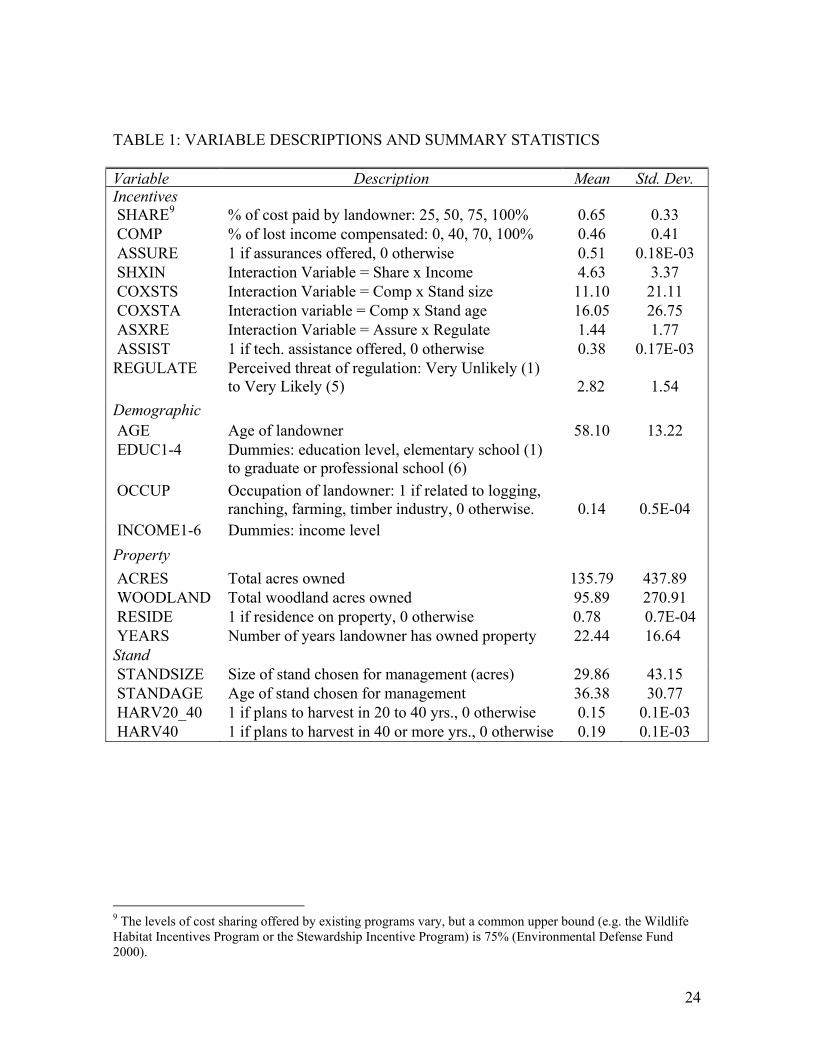
TABLE 1: VARIABLE DESCRIPTIONS AND SUMMARY STATISTICS

Variable Description Mean Std. Dev.Incentives SHARE9 % of cost paid by landowner: 25, 50, 75, 100% 0.65 0.33 COMP % of lost income compensated: 0, 40, 70, 100% 0.46 0.41 ASSURE 1 if assurances offered, 0 otherwise 0.51 0.18E-03 SHXIN Interaction Variable = Share x Income 4.63 3.37 COXSTS Interaction Variable = Comp x Stand size 11.10 21.11 COXSTA Interaction variable = Comp x Stand age 16.05 26.75 ASXRE Interaction Variable = Assure x Regulate 1.44 1.77 ASSIST 1 if tech. assistance offered, 0 otherwise 0.38 0.17E-03 REGULATE Perceived threat of regulation: Very Unlikely (1)

to Very Likely (5) 2.82

1.54

Demographic AGE Age of landowner 58.10 13.22 EDUC1-4 Dummies: education level, elementary school (1)

to graduate or professional school (6)

OCCUP Occupation of landowner: 1 if related to logging, ranching, farming, timber industry, 0 otherwise.

0.14

0.5E-04

INCOME1-6 Dummies: income level Property ACRES Total acres owned 135.79 437.89 WOODLAND Total woodland acres owned 95.89 270.91 RESIDE 1 if residence on property, 0 otherwise 0.78 0.7E-04 YEARS Number of years landowner has owned property 22.44 16.64 Stand STANDSIZE Size of stand chosen for management (acres) 29.86 43.15 STANDAGE Age of stand chosen for management 36.38 30.77 HARV20_40 1 if plans to harvest in 20 to 40 yrs., 0 otherwise 0.15 0.1E-03 HARV40 1 if plans to harvest in 40 or more yrs., 0 otherwise 0.19 0.1E-03

9 The levels of cost sharing offered by existing programs vary, but a common upper bound (e.g. the Wildlife Habitat Incentives Program or the Stewardship Incentive Program) is 75% (Environmental Defense Fund 2000).

25

TABLE 2: ORDERED PROBIT MAXIMUM LIKELIHOOD ESTIMATES

Variable MODEL 1 MODEL 2 Constant -0.26 -0.27

SHARE -0.03 -0.04 (-0.50) (-0.75)

COMP 0.24*** 0.25*** (4.11) (4.22)

ASSURE 0.31*** 0.33*** (4.40) (4.58)

SHXIN 0.02** 0.02** (2.25) (2.40)

COXSTS -0.65E-03 -0.72E-03 (-1.02) (-1.15)

COXSTA -0.74E-03 -0.74E-03 (-1.15) (-1.18)

ASXRE 0.82E-02 0.71E-02 (0.64) (0.55)

ASSIST 0.83E-03 0.01 (0.06) (0.70)

REGULATE -0.56E-02 -0.55E-02 (-0.47) (-0.46)

AGE -0.17E-03 (-0.24)

EDUC2 -0.03 (-1.56)

EDUC3 0.67E-02 (0.37)

EDUC4 -0.46E-02 (-0.22)

OCCUP -0.01 (-0.52)

INCOME2 0.04 0.04 (1.27) (1.29)

INCOME3 0.05 0.05 (1.36) (1.25)

INCOME4 0.03 0.02 (0.55) (0.36)

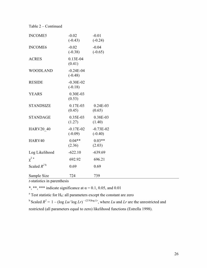
26

Table 2 – Continued INCOME5 -0.02 -0.01 (-0.43) (-0.24)

INCOME6 -0.02 -0.04 (-0.38) (-0.65)

ACRES 0.13E-04 (0.41)

WOODLAND -0.24E-04 (-0.48)

RESIDE -0.30E-02 (-0.18)

YEARS 0.30E-03 (0.53)

STANDSIZE 0.17E-03 0.24E-03 (0.45) (0.65)

STANDAGE 0.35E-03 0.38E-03 (1.27) (1.40)

HARV20_40 -0.17E-02 -0.73E-02 (-0.09) (-0.40)

HARV40 0.04** 0.03** (2.36) (2.03)

Log Likelihood -622.10 -639.69

χ2 a 692.92 696.21

Scaled R2 b 0.69 0.69 Sample Size 724 739 t-statistics in parenthesis

*, **, *** indicate significance at α = 0.1, 0.05, and 0.01 a Test statistic for H0: all parameters except the constant are zero b Scaled R2 = 1 – (log Lu/ log Lr) – (2/N)log Lr, where Lu and Lr are the unrestricted and

restricted (all parameters equal to zero) likelihood functions (Estrella 1998).

27

TABLE 3: SIGNS OF MARGINAL EFFECTS FOR COMP AND ASSURE ∆Pr(PLAN=0) ∆Pr(PLAN=1) ∆Pr(PLAN=2) ∆Pr(PLAN=3) COMP – – + +

ASSURE – – + +

TABLE 4: SIMULATED CHOICE PROBABILITIES

Prob. (Plan 0)

Prob. (Plan 1)

Prob. (Plan 2)

Prob. (Plan 3)

Scenario 0: No Incentives 0.89 0.10 0.01 0.00

Scenario 1: Cost Sharing 0.67 0.10 0.05 0.18

Scenario 2: Compensation 0.35 0.48 0.13 0.04

Scenario 3: Assurances 0.00 0.20 0.78 0.02

Scenario 4: Cost Sharing + Assurances

0.20

0.40

0.22

0.18

Scenario 5: Compensation+ Assurances

0.00

0.00

0.00

1.00

28

REFERENCES

Bean, M. 1998. “The Endangered Species Act and Private Land: Four Lessons Learned from the Past Quarter Century”, Environmental Law Reporter 28. Bean, M. and D. Wilcove. 1996. “Ending the Impasse”, The Environmental Forum, July/August: 22-28. Bean, M. and D.Wilcove. 1997. “The Private Land Problem”, Conservation Biology 11:1-2. Bourland, T. and R. Stroup. 1996. “Rent Payments as Incentives: Making Endangered Species Welcome on Private Land”, Journal of Forestry 96: 18-21. Boyd, R. 1984. “Government Support of Nonindustrial Production: The Case of Private Forests”, Southern Economics Journal 51, July: 89-107. Cooper, J. C. and C. T. Osborn. 1998. “The Effect of Rental Rates on the Extension of Conservation Reserve Program Contracts”, American Journal of Agricultural Economics 80(1): 184-195. Defenders of Wildlife. 1994. Building Economic Incentives into the Endangered Species Act, 3rd ed. Washington, D.C.: Defenders of Wildlife. Dillman, D. A. 1978. Mail and Telephone Surveys. The Total Design Method. New York: John Wiley & Sons. Edwards, S.F. and G. D. Anderson. 1987. “Overlooked Biases in Contingent Valuation Surveys: Some Considerations”, Land Economics 63(2): 168-178. Environmental Defense Fund. Conservation Incentives. Helping Landowners Help Endangered Species. www.environmentaldefense.org.Visited August 22, 2000. Estrella, A. 1998. “A New Measure of Fit for Equations With Dichotomous Dependent Variables”, Journal of Business & Economic Statistics 16(2): 198-205. Greene, W. H. 2000. Econometric Analysis. 4th Ed. Upper Saddle River: Prentice Hall. Hardie, I. and P. Parks. 1996. “Program Enrollment and Acreage Response to Reforestation Cost-Sharing Programs”, Land Economics 72(2): 248-260. Hayes, J. P., S. S. Chan, W. H. Emmingham, J. C. Tappeiner, L. D. Kellog, and J. D. Bailey. 1997 “Wildlife Response to Thinning Young Forests in the Pacific Northwest”, Journal of Forestry, August 1997: 28-33. Heckman, J.J. 1979. “Sample Selection Bias as a Specification Error”, Econometrica 47: 153-161.

29

Innes, R. 2000. “The Economics of Takings and Compensation When Land and Its Public Use Value Are in Private Hands”, Land Economics 76(2): 195-212. Kennedy, E., R. Costa, and W. Smathers Jr. 1996. “Economic Incentives: New Directions for Red-Cockaded Woodpecker Habitat Conservation”, Journal of Forestry 96: 22-26. Keystone Center, The. 1995. Dialogue on Incentives to Protect Endangered Species on Private Lands: Final Report. Keystone, Colorado. Kline, J., Alig, R., and R. Johnson. 2000. “Forest Owner Incentives to Protect Riparian Habitat”, Ecological Economics 33(1): 29-43. Kluender, R. A., T. L. Walkingstick, and J. C. Pickett. 1999. “The Use of Forestry Incentives by Nonindustrial Forest Landowner Groups: Is It Time for a Reassessment of Where We Spend Our Tax Dollars?”, Natural Resources Journal 39: 799-818. Langpap, C. and J. Wu. 2002. “Voluntary Conservation of Endangered Species: When Does ‘No Surprises’ Mean No Conservation?”, Working paper, Dept. of Ag. and Resource Economics, Oregon State University. Long, J. S. 1997. Regression Models for Categorical and Limited Dependent Variables. Thousand Oaks: Sage Publications. Mann, C. and M. Plummer. 1995. Noah’s Choice. The Future of Endangered Species. New York: Alfred A. Knopf. McLean-Meyinsse, P. E., J. Hui, and R. Joseph, Jr. 1994. “An Empirical Analysis of Louisiana Small Farmers’ Involvement in the Conservation Reserve Program”, Journal of Agricultural and Applied Economics 26(2): 379-385. Messonier, M. L., J. C. Bergstrom, C. M. Cornwell, R. J. Teasley, and H. K. Cordell. 2000. “Survey Response-Related Biases in Contingent valuation: Concepts, Remedies, and Empirical Application to Valuing Aquatic Plant Management”, American Journal of Agricultural Economics 83: 438-450. Michael, J. and D. Lueck. 2000. “Preemptive Habitat Destruction Under the Endangered Species Act: The Case of the Red-Cockaded Woodpecker”. Working Paper, Montana State University. Mitchell, R. C. and R. T. Carson. 1989. Using Surveys to Value Public Goods: The Contingent Valuation Method. Washington, DC: Resources for the Future. Polasky, S. 2001. “Investment, Information Collection, and Endangered Species Conservation on Private Land”, in J. Shogren and J. Tschirhart (Eds.), Protecting Endangered Species in the United States: Biological Needs, Political Realities, and Economic Choices. Cambridge: Cambridge University Press.

30

Polasky, S. and H. Doremus. 1998. “When the Truth Hurts: Endangered Species Policy on Private Land with Imperfect Information”, Journal of Environmental Economics and Management 35: 22-47. Royer, J.P. 1987. “Determinants of Reforestation Behavior Among Southern Landowners”, Forest Science 33 (3): 654-667. Smith, R. B. W. 1995. “The Conservation reserve Program as a Least-Cost Land Retirement Mechanism”, American Journal of Agricultural Economics 77(1): 93-105. Smith, R. B. W. and J. F. Shogren. 2001. “Protecting Species on Private Land”, in J. Shogren and J. Tschirhart (Eds.), Protecting Endangered Species in the United States: Biological Needs, Political Realities, and Economic Choices, Cambridge: Cambridge University Press. Smith, R. B. W. and J. F. Shogren. 2002. “Voluntary Incentive Design for Endangered Species Protection”, Journal of Environmental Economics and Management 43: 169-187. Stone, R. 1995. “Incentives Offer Hope for Habitat”, Science 269: 1212-1213. U. S. Department of Agriculture. 1993. Forest Ecosystem Management: An Ecological, Economic, and Social Assessment. Report of the Forest Ecosystem Management Assessment Team. U.S. Fish and Wildlife Service. 1992. Recovery Plan for the Northern Spotted Owl – Draft. Washington, D.C.: Government Printing Office. U.S. Fish and Wildlife Service. 1997a. News release, June 6, 1997.

U. S. Fish and Wildlife Service. 1997b. Recovery Plan for the Threatened Marbled Murrelet in Washington, Oregon, and California. Washington, D.C.: Government Printing Office. Vickerman, S. 1998. Stewardship Incentives. Conservation Strategies for Oregon’s Working Landscape. Washington, DC: Defenders of Wildlife. Wilcove, D., M. Bean, R. Bonnie, and M. McMillan. 1996. “Rebuilding the Ark: Toward a More Effective Endangered Species Act for Private Land”, www.edf.org. Environmental Defense Fund.

Wu, J. and B. Babcock. 1996. “Contract Design and the Purchase of Environmental Goods from Agriculture”, American Journal of Agricultural Economics 78(4): 935-945.

Zhang, D. and W. A. Flick. 2001. “Stick, Carrots, and Reforestation Investment”, Land Economics 77(3): 443-456.