CONSERVATION FORMULATION FLOW AT ALL · PDF fileNumerical Heat Transfer, Part B: Fundamentals,...

Full Terms & Conditions of access and use can be found athttp://www.tandfonline.com/action/journalInformation?journalCode=unhb20

Download by: [American University of Beirut] Date: 05 July 2017, At: 07:35

Numerical Heat Transfer, Part B: Fundamentals

ISSN: 1040-7790 (Print) 1521-0626 (Online) Journal homepage: http://www.tandfonline.com/loi/unhb20

PRESSURE-BASED ALGORITHMS FOR MULTIFLUIDFLOW AT ALL SPEEDS—PART I: MASSCONSERVATION FORMULATION

F. Moukalled & M. Darwish

To cite this article: F. Moukalled & M. Darwish (2004) PRESSURE-BASED ALGORITHMS FORMULTIFLUID FLOW AT ALL SPEEDS—PART I: MASS CONSERVATION FORMULATION,Numerical Heat Transfer, Part B: Fundamentals, 45:6, 495-522, DOI: 10.1080/10407790490430651

To link to this article: http://dx.doi.org/10.1080/10407790490430651

Published online: 17 Aug 2010.

Submit your article to this journal

Article views: 119

View related articles

Citing articles: 10 View citing articles

http://www.tandfonline.com/action/journalInformation?journalCode=unhb20

http://www.tandfonline.com/loi/unhb20

http://www.tandfonline.com/action/showCitFormats?doi=10.1080/10407790490430651

http://dx.doi.org/10.1080/10407790490430651

http://www.tandfonline.com/action/authorSubmission?journalCode=unhb20&show=instructions

http://www.tandfonline.com/action/authorSubmission?journalCode=unhb20&show=instructions

http://www.tandfonline.com/doi/mlt/10.1080/10407790490430651

http://www.tandfonline.com/doi/mlt/10.1080/10407790490430651

http://www.tandfonline.com/doi/citedby/10.1080/10407790490430651#tabModule

http://www.tandfonline.com/doi/citedby/10.1080/10407790490430651#tabModule

PRESSURE-BASED ALGORITHMS FOR MULTIFLUIDFLOW AT ALL SPEEDS—PART I: MASS CONSERVATIONFORMULATION

F. Moukalled and M. DarwishAmerican University of Beirut, Faculty of Engineering & Architecture,Mechanical Engineering Department, Riad El Solh,Beirut, Lebanon

In this article, seven segregated single-fluid, pressure-based algorithms are extended to

predict multifluid flow at all speeds. The extended algorithms form part of the mass con-

servation-based algorithms (MCBA) group, in which the pressure-correction equation is

derived from overall mass conservation. The performance and accuracy of these algorithms

are assessed by solving a variety of two-dimensional two-phase flow problems in the sub-

sonic, transsonic, and supersonic regimes. Solutions are generated for several grid densities

using the single-grid (SG), the prolongation-grid (PG), and the full nonlinear multigrid

(FMG) methods, and their effects on convergence behavior are studied. The main outcomes

of this study are clear demonstrations of: (1) the capability of all MCBA algorithms to deal

with multifluid flow situations; (2) the ability of the FMG method to tackle the added

nonlinearity of multifluid flows; (3) and the capacity of the MCBA algorithms to predict

multifluid flow at all speeds. Moreover, results indicate that the performances of SIMPLE,

SIMPLEC, and SIMPLEX are very close. The PRIME algorithm is the most expensive, due

to the explicit treatment of the fluidic momentum equations. The PISO algorithm is gen-

erally more expensive than SIMPLE. In terms of CPU effort, SIMPLEM stands between

PRIME and SIMPLE. For all algorithms, use of the PG and FMG methods speeds up

acceleration, with the FMG method being more efficient at accelerating the convergence

rate, for the problems solved on the densest grid used, over the SG method, by a factor

reaching a value as high as 6.55.

INTRODUCTION

Since its development over three decades ago, the SIMPLE (Semi-ImplicitMethods for Pressure Linked Equations) algorithm of Patankar and Spalding [1, 2],originally derived for incompressible single-fluid flow, has witnessed a consistent andsustained research effort by many workers. In an attempt to improve its performancein simulating incompressible flows, several variations of this algorithm emerged (e.g.SIMPLEC [3], SIMPLEM [4], SIMPLEX [5], SIMPLEST [6], PISO [7], and PRIME[8] to cite a few), and their collection has been denoted by the computational fluid

Received 29 August 2003; accepted 6 November 2003.

Address correspondence to F. Moukalled, American University of Beirut, Faculty of Engineering

& Architecture, Mechanical Engineering Department, P. O. Box 11–0236, Riad El Solh, Beirut 1107 2020,

Lebanon. E-mail: [email protected]

Numerical Heat Transfer, Part B, 45: 495–522, 2004

Copyright # Taylor & Francis Inc.

ISSN: 1040-7790 print/1521-0626 online

DOI: 10.1080/10407790490430651

495

dynamics (CFD) community as the SIMPLE family. However, none of these algo-rithms could be singled out as being universally the best. Rather, their performancewas shown to be problem and even grid dependent. To further enhance theperformance of the pressure-based approach, CFD researchers sought otheralternatives, among which the multigrid technique proved to be promising, withgrid-independent convergence characteristics. Consequently, some algorithms in theSIMPLE family were implemented within multigrid strategies [9–12] and resulted insubstantial acceleration in the convergence rate for incompressible flow [13],undoubtedly qualifying them as efficient smoothers in multigrid calculations [14].

Due to its advantages over the density-based technique, the pressure-basedapproach was the focus of further developments to extend its use for predicting fluidflow in the various Reynolds and Mach number regimes. These efforts culminated inseveral extended versions of the SIMPLE algorithm that are capable of solving

NOMENCLATURE

AðkÞP ; . . . coefficients in the discretized

equation for fðkÞ

BðkÞP source term in the discretized

equation for fðkÞ

BðkÞ body force per unit volume of

fluid=phase k

CðkÞr coefficient equals to 1=RðkÞT ðkÞ

DðkÞP ½fðkÞ� the matrix D operator

HP½fðkÞ� the H operator

HP½uðkÞ� the vector form of the H operator

IðkÞ interphase momentum transfer

JðkÞDf diffusion flux of fðkÞ across cell face f

JðkÞCf convection flux of fðkÞ across cell

face f_MMðkÞ mass source per unit volume

P pressure

PrðkÞ; PrðkÞt laminar and turbulent Prandtl

number of fluid=phase k

_qqðkÞ heat generated per unit volume of

fluid=phase k

QðkÞ general source term of fluid=phase k

rðkÞ volume fraction of fluid=phase k

RðkÞ gas constant for fluid=phase k

Sf surface vector

t time

TðkÞ temperature of fluid=phase k

uðkÞ velocity vector of fluid=phase k

u(k), v(k) velocity components of fluid=phase k

in x and y directions, respectively

UðkÞf interface flux velocity v

ðkÞf _ Sf

� �of

fluid=phase k

bðkÞ thermal expansion coefficient for

phase=fluid k

GðkÞ diffusion coefficient of fluid=phase k

dt time step

DP fðkÞh i

the D operator

mðkÞ; mðkÞt laminar and turbulent viscosity of

fluid=phase k

rðkÞ density of fluid=phase k

fðkÞ general scalar quantity associated

with fluid=phase k

FðkÞ dissipation term in energy equation

of fluid=phase k

O cell volume

Subscripts

E refers to energy equation

k refers to turbulent kinetic energy

equation

nb refers to the east, west, . . . face of a

control volume

NB refers to the East, West, . . .

neighbors of the main grid point

M refers to momentum equation

P refers to the P grid point

e refers to turbulent eddy diffusivity

equation

Superscripts

C refers to convection contribution

D refers to diffusion contribution

(k) refers to fluid=phase k

ðkÞ� refers to updated value at the current

iteration

ðkÞ� refers to values of fluid=phase k from

the previous iteration

ðkÞ0 refers to correction field of

phase=fluid k

Old refers to values from the previous

time step

496 F. MOUKALLED AND M. DARWISH

single-fluid flow problems at all speeds [15–21]. A unified formulation of the SIM-PLE family of algorithms for the prediction of incompressible and compressiblesingle-fluid flow at all speeds was presented by Moukalled and Darwish [22], while anassessment of their performance within a single grid, a prolongation grid, and a fullmultigrid methodology was recently carried out by Darwish et al. [23].

In parallel with developments in single-fluid flow algorithms, researchers haveexploited the pressure-based method to predict incompressible multiphase flow (e.g.,[24–29]). However, unlike the substantial effort spent on developing variations of thesingle-fluid SIMPLE algorithm, work on multifluid flow algorithms concentratedmostly on the SIMPLE, SIMPLEC, and to a lesser extent PISO, with no attentiongiven to other algorithms, and developments were confined to incompressibleapplications. The first article dealing with pressure-based algorithms for the pre-diction of multifluid flow at all speeds was the one reported by Darwish et al. [30]. Intheir work, it was shown that a multifluid pressure-correction equation can bederived either from the overall mass conservation equation or from the geometricconservation equation. Depending on the route followed, the resulting multifluidalgorithms were denoted either mass conservation-based algorithms (MCBA) orgeometric conservation-based algorithms (GCBA), respectively.

Assessments of performance in one-dimensional space of the incompressiblemultifluid versions of the SIMPLE families were reported by Moukalled andDarwish [31, 32]. Moreover, Moukalled et al. [33] extended the MCBA-SIMPLEalgorithm to predict multifluid flow at all speeds, while Darwish et al. [34] extendedthe work of Moukalled et al. [33] into a multigrid framework. With the exception ofMCBA-SIMPLE, the MCBA and GCBA families have not been implemented orsystematically tested for the prediction of multifluid flow at all speeds. It is theintention of this and a companion article [35] to perform these tasks and implementboth families within a single-grid (SG), a prolongation-grid (PG), and a full multi-grid (FMG) method.

In what follows, the governing equations for multifluid flow are introducedalong with a brief description of the discretization procedure. Then the MCBAapproach is outlined, the FMG and PG methods introduced, the capability of theMCBA algorithms to predict multifluid flow phenomena at all speeds demonstrated,and their performance characteristics (in terms of convergence history and speed)assessed. For that purpose, two incompressible, turbulent, two-phase flow problemsand two compressible two-phase flow problems encompassing dilute and dense gas–solid and bubbly flows in the subsonic, transonic, and supersonic regimes are solved.In addition, the performance of these algorithms using a single grid, a prolongationgrid, and a full multigrid method is compared.

THE GOVERNING EQUATIONS

The equations governing multifluid flows are the conservation laws of mass,momentum, and energy for each individual fluid, which can be written for the kthfluid=phase as

q rðkÞrðkÞ� �

qtþ H_ rðkÞrðkÞuðkÞ

� �¼ rðkÞ _MMðkÞ ð1Þ

MULTIFLUID FLOW—I: MASS CONSERVATION 497

q rðkÞrðkÞuðkÞ� �

qtþ H_ rðkÞrðkÞuðkÞuðkÞ

� �¼ H_ rðkÞðmðkÞ þ mðkÞt ÞHuðkÞ

h i

þ rðkÞ �HPþ BðkÞ� �

þ IðkÞM ð2Þ

q rðkÞrðkÞTðkÞ� �qt

þ H_ rðkÞrðkÞuðkÞTðkÞ� �

¼ H_ rðkÞmðkÞ

PrðkÞþ mðkÞt

PrðkÞt

!HTðkÞ

" #þ rðkÞ

cðkÞP

��bðkÞTðkÞ qP

qtþ H_ PuðkÞ

� �� PH_ uðkÞ

� ��

þ FðkÞ þ _qqðkÞ�þ I

ðkÞE

cðkÞP

ð3Þ

where the superscript (k) refers to the kth fluid and other parameters are as defined inthe Nomenclature. Moreover, the mass sources on the right-hand side of Eq. (1) areoften nonzero, as when one fluid is transformed to another fluid. However, sum-mation over all fluids leads to the following ‘‘global mass conservation’’ equation,which is used in deriving the pressure-correction equation in the mass conservationformulation:

Xk

q rðkÞrðkÞ� �

qtþ H_ rðkÞrðkÞuðkÞ

� � !¼ 0 ð4Þ

For high Reynolds number multifluid flow, several models have been adver-tised for incorporating the effect of turbulence on interfacial mass, momentum, andenergy transfer, which vary in complexity from simple algebraic models [36] to state-of-the-art Reynolds-stress models [37]. However, the widely used multiphase tur-bulence model, adopted in this work, is the two-equation k–e model [38], in whichthe fluidic conservation equations governing the turbulence kinetic energy (k) andturbulence dissipation rate (e) for the kth fluid are given by

q rðkÞrðkÞkðkÞ� �

qtþ H_ rðkÞrðkÞuðkÞkðkÞ

� �

¼ H_ rðkÞmðkÞt

sðkÞk

HkðkÞ !

þ rðkÞrðkÞ GðkÞ � eðkÞ� �

þ IðkÞk ð5Þ

q rðkÞrðkÞeðkÞ� �

qtþ H_ rðkÞrðkÞuðkÞeðkÞ

� �

¼ H_ rðkÞmðkÞt

sðkÞe

HeðkÞ !

þ rðkÞrðkÞeðkÞ

kðkÞc1eG

ðkÞ � c2eeðkÞ� �

þ IðkÞe ð6Þ

where IðkÞk and I

ðkÞe represent the interfacial turbulence terms. The turbulent viscosity

is calculated as


mðkÞt ¼ Cmr kð Þ kðkÞ� �2eðkÞ

ð7Þ

For two-phase flow, several extensions of the k–e model that are based oncalculating the turbulent viscosity by solving the k and e equations for the carrier orcontinuous phase only have been proposed in the literature [39–45]. Due to the lackof better well-developed alternatives, this approach is adopted in this work.

A review of the above differential equations reveals that they are similar instructure. If a typical representative variable associated with phase (k) is denoted byf(k), the general fluidic differential equation may be written as

q rðkÞrðkÞfðkÞ� �

qtþ H_ rðkÞrðkÞuðkÞfðkÞ

� �¼ H_ rðkÞGðkÞHfðkÞ

� �þ rðkÞQðkÞ ð8Þ

where the expressions for G(k) and Q(k) can be deduced from the parent equations.The above set of differential equations has to be solved in conjunction with

constraints on certain variables represented by algebraic relations. These auxiliaryrelations include the equations of state, the geometric conservation equation, and theinterfacial mass, momentum, energy, and turbulence energy transfers. Detailsregarding the auxiliary relations and closures used in this work were reported in[33, 34] and are not repeated here, for compactness.

DISCRETIZATION PROCEDURE

The first step consists of integrating the general conservation equation [Eq. (8)]over a finite cell (Figure 1a) of volume O to yield

ZZO

q rðkÞrðkÞfðkÞ� �

qtdOþ

ZZOH_ rðkÞrðkÞuðkÞfðkÞ� �

dO ¼ZZ

OH_ rðkÞGðkÞHfðkÞ� �

dO

þZZ

OrðkÞQðkÞ dO ð9Þ

Using the divergence theorem to transform the volume integral into a surface inte-gral and then replacing the surface integral by a summation of the fluxes over thesides of the control volume, Eq. (9) is transformed to

q rðkÞrðkÞfðkÞO� �

qtþXnb

JðkÞDnb þ J

ðkÞCnb

� �¼ rðkÞQðkÞO ð10Þ

where JðkÞDnb and J

ðkÞCnb are the diffusive and convective fluxes, respectively. The dis-

cretization of the diffusion term is second-order accurate and follows the derivationspresented in [46]. For the convective terms, the high-resolution (HR) SMART [47]scheme is employed, even for calculating interface densities [21], and applied withinthe context of the NVSF methodology [48]. Substituting the face values by their


Figure

1.(a)Controlvolume.

(b)FullmultigridV

cycles.(c)Theprolongation-only

strategy.(d)TheMG

strategy.(e)Prolongationandrestriction.

500

functional relationship relating to the node values of f, Eq. (10) is transformed aftersome algebraic manipulations into the following discretized equation:

AðkÞP fðkÞ

P ¼XNB

AðkÞNBf

ðkÞNB þ B

ðkÞP ð11Þ

where the coefficients AðkÞP and A

ðkÞNB depend on the selected scheme and B

ðkÞP is the

source term of the discretized equation . In compact form, the above equation can bewritten as

fðkÞ ¼ HP fðkÞh i

¼X

NB

AðkÞNBf

ðkÞNB þ B

ðkÞP

A

ðkÞP

.ð12Þ

In a similar manner, the discretized form of the momentum equation can be writtenas

uðkÞP ¼ HP uðkÞ

h i� rðkÞD

ðkÞP HP Pð Þ ð13Þ

THE MCBA PRESSURE-CORRECTION EQUATION

The number of equations describing an n-fluid flow situation is: n fluidicmomentum equations, n fluidic volume fraction (or mass conservation) equations, ageometric conservation equation, and for the case of a compressible flow an addi-tional n auxiliary pressure–density relations. Moreover, the variables involved arethe n fluidic velocity vectors, the n fluidic volume fractions, the pressure field, and fora compressible flow an additional n unknown fluidic density fields. In all MCBAalgorithms, the n momentum equations are used to calculate the n velocity fields,n7 1 volume fraction (mass conservation) equations are employed to calculate n7 1volume fraction fields, and the last volume fraction field is calculated utilizing thegeometric conservation equation

rðnÞ ¼ 1�Xk 6¼n

rðkÞ ð14Þ

The remaining volume fraction equations can be used to calculate the sharedpressure field, which does not have an explicit equation. However, instead of usingthis last volume fraction equation, the global mass conservation equation [Eq. (4)] isemployed in combination with the fluidic momentum equations, to derive a pressure-correction equation. For that purpose, a guessed pressure field P �ð Þ is substitutedinto the momentum equations. The resulting velocity fields, denoted by uðkÞ

�, which

now satisfy the momentum equations, will not, in general, satisfy the mass con-servation equations. Thus, corrections are needed in order to yield velocity, pressure,and density fields that satisfy both sets of equations. Denoting the corrections forpressure, velocity, and density by P0, uðkÞ

0, and rðkÞ

0, respectively, the corrected fields

are written as

P ¼ P� þ P 0 uðkÞ ¼ uðkÞ�þ uðkÞ

0rðkÞ ¼ rðkÞ

�þ rðkÞ

0ð15Þ

Hence the equations solved in the predictor stage are


uðkÞ�P ¼ HP uðkÞ

��

� rðkÞ�P D

ðkÞP HPP

� ð16Þ

While the final solutions satisfy

uðkÞP ¼ HP uðkÞ

� �� r

ðkÞ�P D

ðkÞP HPP ð17Þ

Subtracting the two equation sets [(16) and (17)] from each other yields the followingequation involving the correction terms:

uðkÞ0P ¼ HP uðkÞ

0� �

� rðkÞ�P D

ðkÞP HPP

0 ð18Þ

Moreover, the new density and velocity fields, r(k) and u(k), will satisfy the overallmass conservation equation if

Xk

rðkÞ�P rðkÞP

� �� r

ðkÞP rðkÞP

� �Old

dtOP þ DP rðkÞ�rðkÞuðkÞ:S

� �264

375 ¼ 0 where

DPðFÞ ¼Xnb

F ð19Þ

Linearizing the (r(k)u(k)) term, one gets

rðkÞ�þ rðkÞ

0� �

uðkÞ�þ uðkÞ

0� �

¼ rðkÞ�uðkÞ

�þ rðkÞ

�uðkÞ

0þ rðkÞ

0uðkÞ

�þ rðkÞ

0uðkÞ

0ð20Þ

Substituting Eqs. (20) and (18) into Equation (19), rearranging, and replacing den-sity correction by pressure correction, the final form of the pressure-correctionequation is written as

Xk

(OP

dtrðkÞ�P CðkÞ

r P0P þ DP rðkÞ

�UðkÞ�CðkÞ

r P0� �

� DP rðkÞ�rðkÞ

�rðkÞ

�DðkÞHP0

� �:S

h i)

¼ �Xk

rðkÞ�P

rðkÞ�

P� r

ðkÞP

rðkÞPð ÞOld

dt OP þ DP rðkÞ�rðkÞ�UðkÞ��

þDP rðkÞ�rðkÞ

�H uðkÞ

0� �h i

�Sh i

þ DP rðkÞ�rðkÞ0uðkÞ

0:S

� �0BB@

1CCA

ð21Þ

The corrections applied to the velocity, pressure, and density fields are given by

uðkÞ�P ¼ u

ðkÞ�P � r

ðkÞ�P D

ðkÞP HPP

0 P� ¼ P� þ P0 rðkÞ�¼ rðkÞ� þ CðkÞ

r P0 ð22Þ

If the HðuðkÞ0 Þ term in Eq. (21) is retained, there will result a pressure-correctionequation relating the pressure correction value at a point to all values in the domain.To facilitate implementation and reduce cost, simplifying assumptions related to thisterm have been introduced. Depending on these assumptions, different algorithmsare obtained. A summary of the various MCBA algorithms used in this work wasaccorded a full-length article, to which interested reader is referred [30].


The sequence of events in the MCBA is as follows:

1. Solve the fluidic momentum equations for velocities.2. Solve the pressure-correction equation based on global mass conservation.3. Correct velocities, densities, and pressure.4. Solve the fluidic mass conservation equations for volume fractions.5. Solve the fluidic energy equations.6. Return to the first step and repeat until convergence.

THE NONLINEAR MULTIGRID STRATEGY

The above-described procedure applies to a single-grid method, for which therate of convergence is high during the very first iterations but degrades thereafter,and the situation gets worse as the number of grid points increases. This behavior isattributed to the smoothing property of the algorithms [13], which are efficient inremoving only the high-frequency components of the error. The low-frequencycomponents, which have long wavelength compared to the grid spacing, are notproperly resolved. This is clearly noticed when using any of the solvers on pro-gressively denser grids, in which case the convergence rate decreases more rapidly onthe finer grids. The performance of these algorithms can thus be substantiallyimproved by combination with the multigrid method.

In the multigrid approach the high-frequency errors are initially eliminated on thefinest grid, then,when the convergence rate degrades, the process is repeated ona coarsergrid, where part of the low-frequency error components of the finer grid are transformedinto high-frequency error components on the coarser grid, which can be efficientlyremoved. This step is recursively applied on coarser grids, and more of the errorcomponents are reduced. Results are then interpolated back from coarser to finer grids.

The V-cycle multigrid strategy (Figure 1b) adopted in this work starts at thecoarsest level, where the solution is first computed; this solution is interpolated ontothe next finer mesh, where it is used as initial guess. This stage is called the pro-longation stage (see Figure 1c). Then iterations are performed on the fine mesh andthe solution is transferred back to the coarser mesh by applying a restrictionoperator and adding forcing terms so that the truncation errors on both the fine andcoarse grids are of the same order. After performing a number of iterations on thecoarse mesh, the solution is transferred back to the finer mesh in the form of acorrection, and a number of iterations are performed on the finer grid to smooth thefields. This process is continued until a converged solution on the fine mesh isobtained (see Figure 1d ). Then the solution is extrapolated into a finer mesh and theprocess repeated until convergence is reached on the desired finest mesh.

In the restriction step (Figure 1e), the coarse-grid variables are computed fromthe fine-grid values as

~ffC ¼ 1

4

Xi¼1...4

fFiþ HfFi

� dFiC

� �ð23Þ

while in the prolongation step (Figure 1e), the fine-grid corrections are computedfrom the coarse-grid corrections as

f0Fi¼ f0

C þ Hf0C � dCFi

ð24Þ


where

f0C ¼ fC � ~ffC ð25Þ

The special character of the volume fraction and k–e equations necessitatesmodification to the prolongation procedure. For the k–e turbulence model, theremedy suggested by Cornelius et al. [49] is adopted. For the volume-fractionequations, the following treatment is applied: While extrapolating the volume-fraction field from the coarse to the fine grid, the prolongation operator may yieldnegative volume-fraction values or values that are greater than one. Such unphysicalvalues are detrimental to the overall convergence rate and may even cause diver-gence. To circumvent this problem, a simple yet very effective treatment is adopted:Once the r values are extrapolated, a check is performed to make sure they are withinbounds. If any of the r values is found to be unbounded, the r fluidic volume-fractionequation is solved starting with the interpolated values until all of the r values arewithin the set bounds. Typically, fewer than 10 iterations are needed. This treatmenthas been found to be very effective and to preserve the convergence accelerationrate.

In addition to the FMG strategy, the PG approach is also tested. Thisapproach differs from the FMG method in that the solution moves in one directionfrom the coarse to the fine grids, with the initial guess on level nþ 1 obtained byinterpolation from the converged solution on level n (Figure 1c). As such, theacceleration over the SG method obtained with this approach is an indication of theeffect of initial guess on convergence.

RESULTS AND DISCUSSION

The performance of the various multifluid mass conservation-based algorithmsis assessed in this section by presenting solutions to four two-dimensional, two-phaseflow problems. The first two tests deal with incompressible turbulent flows, while thelast two are concerned with compressible flows. As mentioned earlier, solutions areobtained using the prolongation-grid scheme (PG) and the full multigrid method(FMG) in addition to the usual single-grid (SG) approach. Results are presented interms of the CPU time needed to converge the solution to a set level and of theconvergence history. Moreover, solutions are generated for a number of grids inorder to assess the performance of the various algorithms with increasing griddensity. Results are compared against available experimental data and=or numer-ical=theoretical values. The residual of a variable f at the end of an outer iteration isdefined as

RESðkÞf ¼

Xc:v

ApfðkÞp �

Xall p

neighbors

AnbfðkÞnb � BðkÞ

p

��

��ð26Þ

For global mass conservation, the imbalance in mass is given by

RESC ¼Xk

Xc:v:

rðkÞP rðkÞP

� �� r

ðkÞP rðkÞP

� �Old

dtO� DP rðkÞrðkÞuðkÞ �S

h i� rðkÞ _MMðkÞ

�� ð27Þ


All residuals are normalized by their respective inlet fluxes. Computations areterminated when the maximum normalized residuals of all variables drop below avery small number es. In all problems, the first phase represents the continuous phase[denoted by a superscript (c)], which must be fluid, and the second phase is thedisperse phase [denoted by a superscript (d)], which may be solid or fluid. Unlessotherwise specified, the HR SMART scheme is used in all computations reported inthis study. For a given problem, all results are generated starting from the sameinitial guess. Moreover, the computational details of the various problems con-sidered were discussed in [33, 34], to which the reader is referred. Thus, only a briefdescription of the physical phenomena is given here.

Problem 1: Turbulent Upward Bubbly Flow in a Pipe

In this problem, the radial phase distribution of turbulent upward air–waterflow in a pipe is predicted. Many experimental and numerical studies addressing thisproblem have appeared in the literature [33, 34, 50–53]. The case considered herereproduces numerically the experimental data reported by Seriwaza et al. [50], forwhich the Reynolds number based on superficial liquid velocity and pipe diameter is86104, the inlet superficial gas and liquid velocities are 0.077 and 1.36 m=s,respectively, and the inlet void fraction is 5.3661072 with no slip between theincoming phases. Moreover, the bubble diameter is taken as 3mm [53], while thefluid properties are set to r(c)¼ 1,000 kg=m3, r(d)¼ 1.23 kg=m3, and nðcÞl ¼ 1076 m2=s.Predicted radial profiles of the vertical liquid velocity and void fraction presented inFigure 2 using a grid of size 96632 control volumes concur very well with mea-surements [50] and compare favorably with numerical profiles reported by Boissonand Malin [53].

To assess the merits of the various algorithms for such flows, calculations areperformed on four different grids of sizes 1264, 2468, 48616, and 96632 controlvolumes. On each grid, solutions are generated using the SG, PG, and FMG stra-tegies for all algorithms. Results are displayed in the form of (1) total mass residualssummed over both phases as a function of outer iterations, and (2) normalized CPUtime (Table 1) needed for the maximum normalized residuals of all variables and forall phases to drop below es¼ 1076. In order not to overload plots, only residualsover the densest grid using the SG, PG, and FMG methodologies are presented inFigure 3. Moreover, it should be clarified that in the case of PISO (Figure 3a) andPRIME (Figure 3f ), the number of iterations needed to satisfy the convergencecriteria is higher than the one presented (this will be reflected by their respectivenormalized CPU times displayed in Table 1), due to the slower convergence rate ofthe axial liquid momentum and turbulence kinetic energy equations; i.e., the con-vergence rate of these equations is slower than the overall mass conservationequation. Since the overall mass residuals are presented, only the iterations needed todecrease these residuals to the required level (1076) are displayed, even though at thestate of convergence these residuals are much lower (of the order of 1079).

As can be seen from Figure 3, it is possible to converge the solution to thedesired level with all algorithms. With the single-grid method, the SIMPLEMalgorithm (Figure 3d ) requires a considerably larger number of iterations incomparison with SIMPLE. Moreover, the performance of SIMPLE (Figure 3b),


Figure 2. Comparison of fully developed liquid velocity and void fraction profiles for turbulent bubbly

upward bubbly flow in a pipe.

Table 1. Normalized CPU times for turbulent bubbly flow in a pipe

Algorithms

Grid Method SIMPLE SIMPLEC SIMPLEX SIMPLEST SIMPLEM PISO PRIME

1264 C.V. SG 1.00 0.97 0.98 1.02 1.27 0.91 1.62

2468 C.V. SG 3.30 3.43 3.42 3.79 5.54 3.77 5.76

PG (2 levels) 3.62 3.53 3.58 3.97 5.70 3.87 6.21

SG=PG 0.91 0.97 0.95 0.96 0.97 0.97 0.93

FMG (2 levels) 3.10 3.04 3.12 4.68 5.34 8.81 7.06

SG=FMG 1.07 1.13 1.10 0.81 1.04 0.43 0.82

48616 C.V. SG 25.34 25.71 26.19 30.52 49.17 33.43 46.42

PG (3 levels) 21.92 22.37 23.36 24.27 44.43 70.17 85.56

SG=PG 1.16 1.15 1.12 1.26 1.11 0.48 0.54

FMG (3 levels) 14.44 13.55 14.23 21.74 22.02 45.61 45.36

SG=FMG 1.75 1.90 1.84 1.40 2.23 0.73 1.02

96632 C.V. SG 1231.38 1238.38 1296.28 1249.46 2038.94 1934.27 2059.89

PG (4 levels) 978.29 978.84 1037.55 1002.88 1593.90 1730.55 1853.99

SG=PG 1.26 1.27 1.25 1.25 1.28 1.12 1.11

FMG (4 levels) 207.61 208.46 217.84 214.60 836.08 352.91 314.29

SG=FMG 5.93 5.94 5.95 5.82 2.44 5.48 6.55


Figure

3.(a)–(g)Convergence

histories

oftheSG,PG,andFMG

methodsonthefinestgrid,and(h)convergence

histories

ofthevariousalgorithmsonthefinestmesh

usingtheFMG

methodforturbulentupward

bubbly

flow

inapipe.

507

SIMPLEC (Figure 3c), SIMPLEST (Figure 3e), and SIMPLEX (Figure 3g) is veryclose. This is also demonstrated in Figure 3h, where the convergence histories usingthe FMG method are plotted for all algorithms. As shown, the plots for thesealgorithms are hard to distinguish. For all algorithms, the SG requires the largestnumber of iterations and the FMG the lowest number of iterations. The FMGmethod greatly reduces the number of iterations, whereas reduction with the PGmethod is not as significant. As shown in the plots, the rate of convergence of the SGand PG methods diminishes as the iterations proceed. This is in contrast with theconvergence behavior of the FMG method, which seems to maintain, more or less,the same convergence rate (on the finest level) as the iterations progress.

In Table 1, the normalized CPU times required by the different algorithms tosolve the problem on the various grids and with the various methodologies arepresented. In addition, the ratio of the time needed by the SG method to the oneneeded by the PG and the FMG method are displayed. This allows for a directquantitative assessment of their acceleration rate. As depicted, the CPU effortincreases for all methods and algorithms with increasing the grid size. The CPUtimes of SIMPLE, SIMPLEC, SIMPLEX, and SIMPLEST are very close on allgrids and for all methods, with no clear superiority of any algorithm over the others.PISO requires the least computational time on the coarsest grid used (1264 c.v.);however, as the grid size increases, the picture is reversed and its performancedegrades and becomes closer to that of PRIME and SIMPLEM. The use of the PGmethod on the relatively coarse grids increases the computational cost. The benefit ofthe PG method is realized on the relatively dense grids. On the densest grid, thesavings in computational effort varies from 11% for PRIME to 28% for SIMPLEM,with an average acceleration rate for all algorithms of 22%. The use of the FMGmethod is highly beneficial and its virtues generally appear on all grids, with the rateof acceleration increasing with increasing grid density. On the finest grid, the rate ofacceleration varies from 144% for SIMPLEM to 555% for PRIME, with an averageacceleration rate for all algorithms of 444%. This average rate of acceleration isnearly 20 times the one obtained with the PG method. This indicates that thenonlinearity in multifluid flows is properly resolved using the nonlinear multigridmethod.

Problem 2: Turbulent Air–Particle Flow in a Vertical Pipe

The problem consists of predicting the upward flow of a dilute gas–solidmixture in a vertical pipe [54–56]. For these simulations, the axisymmetric form ofthe gas and particulate transport equations are employed. The configuration selectedis the one experimentally investigated by Tsuji et al. [54], for which the pipe diameteris 30.5mm, the Reynolds number based on the pipe diameter is 3.36104, the meanair inlet velocity is 15.6m=s, and the particle diameter and density are 200 mm and1,020 kg=m3, respectively. In the computations, the mass-loading ratio at the inlet isconsidered to be 1, with no slip between the phases. Figure 4 shows the fullydeveloped gas and particle mean axial velocity profiles generated using a grid of size96640C.V. It is evident that there is generally very good agreement between thepredicted and experimental data, with the gas velocity being slightly overpredictedand the particle velocity slightly underpredicted. Moreover, close to the wall, the


model predictions indicate that the particles have higher velocities than the gas,which is in accord with the experimental results of Tsuji et al. [54].

The problem is solved over four different grids of sizes 1265, 24610, 48620,and 96640 control volumes using the SIMPLE, SIMPLEC, SIMPLEX, and SIM-PLEST multifluid algorithms and the SG, PG, and FMG solution methods. Insolving the problem, it is noticed that the initial guess greatly affects the convergencehistory and time required to converge the solution to the desired level. Except whensolving on the finest mesh with the SG method, the initial guess used for the velocityfield is u(c)¼ u(d)¼ 1m=s. The use of this initial value with the SG method on thefinest mesh increased the CPU effort needed by 500% over the one needed whenstarting with an initial field of u(c)¼ u(d)¼ 15.6m=s. To reduce cost, the latter initialguess is used. For this reason the mass residuals start from a somewhat lower valuethan expected. As in the previous problem, results are displayed in the form of (1)total mass residuals summed over both phases as a function of outer iterations(Figure 5), and (2) normalized CPU time (Table 2) needed for the maximum

Figure 4. Comparison of fully developed gas and particle velocity profiles for turbulent air–particle flow in

a pipe.


normalized residuals of all variables and for all phases to drop below es¼ 1076. Inorder not to overload plots, only residuals over the densest grid using the SG, PG,and FMG methodologies are presented. As shown in Figures 5(a)–5(d), the con-vergence histories and the number of iterations required by the various methods andalgorithms are nearly identical. In addition, the PG and FMG methods greatlyreduce the number of iterations, with the number needed by the PG method beingaround four times the number entailed by the FMG method. The slopes of thevarious curves displayed in Figure 5, which are clearly much higher for the FMGmethod, further reveal this.

The normalized CPU times consumed by the four algorithms to solve theproblem on the various grids and with the various methodologies, which are pre-sented in Table 2, indicate an increase with increasing the grid size. On the densegrids, the CPU time required by the four algorithms is very close, with no appre-ciable superiority of any one. Using the PG method on the finest mesh accelerates the

Figure 5. Convergence histories of (a) SIMPLE, (b) SIMPLEC, (c) SIMPLEST, and (d) SIMPLEX

algorithms using the SG, PG, and FMG methods on the finest mesh for turbulent air–particle flow in a

pipe.


convergence by an average factor of 1.24, whereas the FMG does a much better jobof accelerating the solution, by a factor of around 5.

Problem 3: Compressible Dusty Flow over a Flat Plate

This problem has been used by several researchers [57–59] to check theircomputational methodologies and is used here for the same purpose. It is known thattwo-phase flow greatly changes the main features of the boundary layer over a flatplate. Typically, three different regions are defined in the two-phase boundary layer(Figure 6a), which can be distinguished by the relative velocity between thetwo phases: a large-slip region close to the leading edge, a moderate-slip regionfarther down, and a small-slip one far downstream. It has also been established [58]that the characteristic scale in this two-phase flow problem is the relaxation lengthle, defined as

le ¼2

9

rðdÞr2pu1mðcÞ

ð28Þ

where rðdÞ and rp are, respectively, the density and radius of the particles, m(c) is theviscosity of the fluid, and u1 is the free-stream velocity. The three regions are definedaccording to the order of magnitude of the slip parameter x� ¼ x=le. In the simu-lation, the particle diameter is chosen to be 10 mm, the particle Reynolds number isassumed to be equal to 10, and the material density is 1,766 kg=m3. The Prandtlnumber is equal to 0.75. The south wall is treated as a no-slip wall boundary for thegas phase (both components of the gas velocity are set to zero) and a slip wallcondition for the particles phase (the normal fluxes are set to zero). The gas and theparticles enter the computational domain under thermal and dynamical equilibrium

Table 2. Normalized CPU times for turbulent air–particle flow in a pipe

Algorithms

Grid Method SIMPLE SIMPLEC SIMPLEX SIMPLEST

1265 C.V. SG 1.00 0.97 0.99 1.36

24610 C.V. SG 6.75 6.78 7.09 6.9

PG (2 levels) 5.82 5.76 5.93 5.99

SG=PG 1.16 1.18 1.20 1.15

FMG (2 levels) 4.96 4.43 5.18 6.36

SG=FMG 1.36 1.53 1.37 1.08

48620 C.V. SG 73.46 73.11 73.09 71.67

PG (3 levels) 59.41 59.84 62.78 62.75

SG=PG 1.24 1.22 1.16 1.14

FMG (3 levels) 30.28 28.99 30.38 31.37

SG=FMG 2.43 2.52 2.07 2.28

96640 C.V. SG 829.55 831.40 879.20 841.92

PG (4 levels) 657.14 663.89 703.07 701.53

SG=PG 1.26 1.25 1.25 1.20

FMG (4 levels) 164.88 165.76 173.60 171.88

SG=FMG 5.03 5.02 5.06 4.90


Figure 6. The three different regions within the boundary layer of dusty flow over a flat plate. Comparison

of fully developed gas and particle velocity profiles inside the boundary layer at different axial locations for

dilute two-phase flow over a flat plate.


conditions. A mass load ratio of 1 between the particle phase and the gas phase isused.

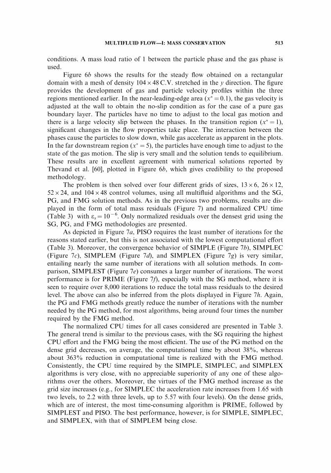
Figure 6b shows the results for the steady flow obtained on a rectangulardomain with a mesh of density 104648C.V. stretched in the y direction. The figureprovides the development of gas and particle velocity profiles within the threeregions mentioned earlier. In the near-leading-edge area (x� ¼ 0.1), the gas velocity isadjusted at the wall to obtain the no-slip condition as for the case of a pure gasboundary layer. The particles have no time to adjust to the local gas motion andthere is a large velocity slip between the phases. In the transition region (x� ¼ 1),significant changes in the flow properties take place. The interaction between thephases cause the particles to slow down, while gas accelerate as apparent in the plots.In the far downstream region (x� ¼ 5), the particles have enough time to adjust to thestate of the gas motion. The slip is very small and the solution tends to equilibrium.These results are in excellent agreement with numerical solutions reported byThevand et al. [60], plotted in Figure 6b, which gives credibility to the proposedmethodology.

The problem is then solved over four different grids of sizes, 1366, 26612,52624, and 104648 control volumes, using all multifluid algorithms and the SG,PG, and FMG solution methods. As in the previous two problems, results are dis-played in the form of total mass residuals (Figure 7) and normalized CPU time(Table 3) with es¼ 1076. Only normalized residuals over the densest grid using theSG, PG, and FMG methodologies are presented.

As depicted in Figure 7a, PISO requires the least number of iterations for thereasons stated earlier, but this is not associated with the lowest computational effort(Table 3). Moreover, the convergence behavior of SIMPLE (Figure 7b), SIMPLEC(Figure 7c), SIMPLEM (Figure 7d), and SIMPLEX (Figure 7g) is very similar,entailing nearly the same number of iterations with all solution methods. In com-parison, SIMPLEST (Figure 7e) consumes a larger number of iterations. The worstperformance is for PRIME (Figure 7f), especially with the SG method, where it isseen to require over 8,000 iterations to reduce the total mass residuals to the desiredlevel. The above can also be inferred from the plots displayed in Figure 7h. Again,the PG and FMG methods greatly reduce the number of iterations with the numberneeded by the PG method, for most algorithms, being around four times the numberrequired by the FMG method.

The normalized CPU times for all cases considered are presented in Table 3.The general trend is similar to the previous cases, with the SG requiring the highestCPU effort and the FMG being the most efficient. The use of the PG method on thedense grid decreases, on average, the computational time by about 38%, whereasabout 363% reduction in computational time is realized with the FMG method.Consistently, the CPU time required by the SIMPLE, SIMPLEC, and SIMPLEXalgorithms is very close, with no appreciable superiority of any one of these algo-rithms over the others. Moreover, the virtues of the FMG method increase as thegrid size increases (e.g., for SIMPLEC the acceleration rate increases from 1.65 withtwo levels, to 2.2 with three levels, up to 5.57 with four levels). On the dense grids,which are of interest, the most time-consuming algorithm is PRIME, followed bySIMPLEST and PISO. The best performance, however, is for SIMPLE, SIMPLEC,and SIMPLEX, with that of SIMPLEM being close.


Figure

7.(a)–(g)Convergence

histories

oftheSG,PG,andFMG

methodsonthefinestgrid,and(h)convergence

histories

ofthevariousalgorithmsonthefinestmesh

usingtheFMG

methodfordustygasflow

over

aflatplate.

514

Problem 4: Inviscid Transsonic Dusty Flow in a Converging-DivergingNozzle

The final test deals with dilute two-phase supersonic flow in an axisymmetricconverging-diverging rocket nozzle. Several researchers have analyzed the problem,and data are available for comparison [60–65]. The flow is assumed to be inviscidand the single-phase results are used as an initial guess for solving the two-phase flowproblem. The physical configuration (Figure 8a) and properties used are the onesdescribed in [62]. The gas stagnation temperature and pressure at inlet to the nozzleare 555K and 10.346105N=m2, respectively. The specific heat for the gas andparticles are 1.076103 J=kgK and 1.386103 J=kgK, respectively, and the particledensity is 4,004.62 kg=m3. With a zero inflow velocity angle, the fluid is acceleratedfrom subsonic to supersonic speed in the nozzle. The inlet velocity and temperatureof the particles are presumed to be the same as those of the gas phase. Results for aparticle size of radius 10 mm with a mass fraction f¼ 0.3 are presented using a grid ofsize 188680C.V. Figure 8b shows the particle volume fraction contours, whileFigure 8c displays the velocity distribution. For the particle size selected, a largeparticle-free zone appears due to the inability of these relatively heavy particles(rp¼ 10 mm) to turn around the throat corner. These findings are in excellentagreement with published results reported by Chang et al. [62] and others usingdifferent methodologies. In addition, contours are similar to those reported byChang et al. [62].

A quantitative comparison of current predictions with published experimentaland numerical data is presented in Figure 9 through gas Mach number distributionsalong the wall (Figure 9a) and centerline (Figure 9b) of the nozzle for the one-phaseand two-phase flow situations. As can be seen, the one-phase predictions fall on topof experimental data reported in [63–65]. Due to the unavailability of two-phase flowdata, predictions are compared against the numerical results reported in [62].

Table 3. Normalized CPU times for dusty flow over a flat plate

Algorithms

Grid Method SIMPLE SIMPLEC SIMPLEX SIMPLEST SIMPLEM PISO PRIME

1366 C.V. SG 1.00 0.96 0.99 1.06 1.43 0.74 1.12

26612 C.V. SG 4.06 4.38 4.55 5.31 5.44 3.84 5.75

PG (2 levels) 3.77 3.87 3.73 5.59 4.49 3.02 5.47

SG=PG 1.08 1.13 1.22 0.95 1.21 1.27 1.05

FMG (2 levels) 2.80 2.66 2.69 9.42 3.77 3.31 7.98

SG=FMG 1.45 1.65 1.69 0.56 1.44 1.16 0.72

52624 C.V. SG 30.61 30.69 32.76 43.41 39.45 38.08 62.78

PG (3 levels) 27.22 27.41 29.74 37.92 33.53 35.25 54.02

SG=PG 1.12 1.12 1.10 1.14 1.18 1.08 1.16

FMG (3 levels) 13.52 13.97 14.34 39.07 17.15 23.41 39.17

SG=FMG 2.26 2.20 2.28 1.11 2.30 1.63 1.60

104648 C.V. SG 373.17 375.29 386.01 715.44 423.80 495.72 1295.88

PG (4 levels) 280.69 279.03 286.76 629.68 301.09 423.66 680.36

SG=PG 1.33 1.34 1.35 1.14 1.41 1.17 1.90

FMG (4 levels) 75.74 67.34 70.48 234.00 86.15 154.20 246.60

SG=FMG 4.93 5.57 5.48 3.06 4.92 3.21 5.25


As displayed in Figures 9a and 9b, both solutions are in good agreement with eachother, indicating once more the correctness of the calculation procedures.

As reported in [34], the use of the single-grid method requires a large number ofiterations on the dense grid with heavy underrelaxation, and the performance of the

Figure 8. (a) Physical domain for the dusty gas flow in a converging-diverging nozzle: (b) Volume–fraction

contours and (c, d) particle velocity vectors for dusty gas flow in a converging-diverging nozzle.


Figure 9. Comparison of one-phase and two-phase gas Mach number distributions along (a) wall and (b)

centerline of the dusty flow in a converging-diverging nozzle problem.


FMG is marginally better than that of the PG method. Because of this, the relativeperformance of the SIMPLE, SIMPLEC, SIMPLEX, and SIMPLEST multifluidalgorithms is compared using the PG method only over three different grids of sizes47620, 94640, and 188680C.V. As before, results are displayed in the form oftotal mass residuals (Figure 10) and normalized CPU times (Table 4).

As shown in Figure 10, with the exception of SIMPLEST, which needs about17% more iteration, all algorithms require almost the same number of iterations. As

Figure 10. Convergence histories of (a) SIMPLE, (b) SIMPLEC, (c) SIMPLEST, and (d) SIMPLEX

algorithms using the SG method for dusty gas flow in a converging-diverging nozzle.

Table 4. Normalized CPU times for dusty flow in a converging-diverging nozzle

Algorithms

Grid Method SIMPLE SIMPLEC SIMPLEX SIMPLEST

47620 C.V. SG 1.00 1.05 1.13 1.47

94640 C.V. PG (2 levels) 12.57 12.97 14.06 13.62

188680 C.V. PG (3 levels) 86.64 90.61 98.06 98.53


expected, the number of iterations increases with increasing grid density. Moreover,the convergence histories of all algorithms are nearly identical. The normalized CPUtimes presented in Table 4 confirm these conclusions and reveal the close per-formance of SIMPLE and SIMPLEC. The normalized CPU times needed bySIMPLEX, which are close to SIMPLEST, are higher than those needed by SIMPLEand SIMPLEC due to the additional equations solved. Its performance could improveon denser grids.

CLOSING REMARKS

The implementation of seven MCBA algorithms for the simulation of multi-fluid flow at all speeds was accomplished. The algorithms were embedded within anonlinear full multigrid strategy. A two-fluid k–e model and several interphasemodels were also employed. Solving a variety of two-dimensional two-phase flowproblems assessed the performance and accuracy of these algorithms. For each testproblem, solutions were generated on a number of grid systems using the single-gridmethod (SG), the prolongation-grid method (PG), and the full nonlinear multigridmethod (FMG). Results obtained demonstrated the capability of all algorithms topredict multifluid flow at all speeds and the ability of the FMG method to tackle theadded nonlinearity of laminar and turbulent multifluid flows. The convergencehistory plots and CPU times presented indicated similar performance for SIMPLE,SIMPLEC, and SIMPLEX. The PISO, SIMPLEM, and SIMPLEST algorithmswere generally more expensive than SIMPLE. In general, the PRIME algorithm wasthe most expensive to use. Moreover, the PG and FMG methods accelerated theconvergence rate for all algorithms. The FMG method was found to be by far moreefficient.

REFERENCES

1. S. V. Patankar and D. B. Spalding, A Calculation Procedure for Heat, Mass and

Momentum Transfer in Three-Dimensional Parabolic Flows, Int. J. Heat Mass Transfer,vol. 15, pp. 1787–1806, 1972.

2. S. V. Patankar, Numerical Heat Transfer and Fluid Flow, Hemisphere, New York, 1981.

3. J. P. Van Doormaal and G. D. Raithby, Enhancement of the SIMPLE Method forPredicting Incompressible Fluid Flows, Numer. Heat Transfer, vol. 7, pp. 147–163, 1984.

4. S. Acharya, and F. Moukalled, Improvements to Incompressible Flow Calculation on a

Non-staggered Curvilinear Grid, Numer. Heat Transfer, B, vol. 15, pp. 131–152, 1989.5. J. P. Van Doormaal and G. D. Raithby, An Evaluation of the Segregated Approach for

Predicting Incompressible Fluid Flows, ASME Paper 85-HT-9, Natl. Heat Transfer

Conf., Denver, Co., August 4–7, 1985.6. D. B. Spalding Mathematical Modelling of Fluid Mechanics, Heat Transfer and Mass

Transfer Processes, Mech. Eng. Dept., Rep. HTS=80=1, Imperial College of Science,Technology and Medecine, London, UK, 1980.

7. R. I. Issa, Solution of the Implicit Discretized Fluid Flow Equations by Operator Split-ting, Mech. Eng. Rep. FS=82=15, Imperial College, London, UK, 1982.

8. C. R. Maliska and G. D. Raithby, Calculating 3-D fluid Flows Using Non-orthogonal

Grid, Proc. Third Int. Conf. on Numerical Methods in Laminar and Turbulent Flows,Seattle, WA, 1983, pp. 656–666.


9. C. Becker, J. H. Ferziger, M. Perı́c, and G. Scheurer, Finite Volume Multigrid Solutions

of the Two-Dimensional Incompressible Navier-Stokes Equations, Notes on Numer. FluidMech., vol. 23, pp. 37–47, 1988.

10. K. M. Smith, W. K. Cope, and S. P.Vanka, Multigrid Procedure for Three Dimensional

Flows on Non-orthogonal Collocated Grids, Int. J. Numer. Meth. Fluids, vol. 17, pp. 887–904, 1993.

11. F. S. Lien and M. A. Lechziner, Multigrid Acceleration for Recirculating Laminar andTurbulent Flow Computed on a Non-orthogonal, Collocated Finite Volume Scheme,

Comput. Meth. Appl. Mech. Eng., vol. 118, pp. 351–371, 1994.12. S. Sivaloganathan and G. J. Shaw, An Efficient Non-linear Multigrid Procedure for the

Incompressible Navier-Stokes Equations, Int. J. Numer. Meth. Fluids, vol. 8, pp. 417–440,

1988.13. J. H. Ferziger and M. Peric, Computational Methods for Fluid Dynamics, Springer-Verlag,

Berlin, Heidelberg, 1996.

14. T. Gjesdal and M. E. H. Lossius, Comparison of Pressure Correction Smoothers forMultigrid Solution of Incompressible Flow, Int. J. Numer. Meth. Fluids, vol. 25, pp. 393–405, 1997.

15. I. Demirdzic, Z. Lilek, and M. Peric, A Collocated Finite Volume Method for PredictingFlows at All Speeds, Int. J. Numer. Meth. Fluids, vol. 16, pp. 1029–1050, 1993.

16. C. H. Marchi, and C. R. Maliska, A Non-orthogonal Finite-Volume Method for theSolution of All Speed Flows Using Co-Located Variables, Numer. Heat Transfer, B, vol.

26, pp. 293–311, 1994.17. F. S. Lien and M. A. Leschziner, A Pressure-Velocity Solution Strategy for Compressible

Flow and Its Application to Shock=Boundary-Layer Interaction Using Second-Moment

Turbulence Closure, J. Fluids Eng., vol. 115, pp. 717–725, 1993.18. M. A. Lien and M. A. Leschziner, A General Non-Orthogonal Collocated Finite Volume

Algorithm for Turbulent Flow at All Speeds Incorporating Second-Moment Turbulence-

Transport Closure, Part 1: Computational Implementation, Comput. Meth. Appl. Mech.Eng., vol. 114, pp. 123–148, 1994.

19. K. H. Chen and R. H. Pletcher, Primitive Variable, Strongly Implicit Calculation Pro-cedure for Viscous Flows at All Speeds, AIAA J., vol. 29, no. 8, pp. 1241–1249, 1991.

20. M. Darbandi and G. E. Shneider, Momentum Variable Procedure for Solving Com-pressible and Incompressible Flows, AIAA J., vol. 35, no. 12, pp. 1801–1805, 1997.

21. F. Moukalled and M. Darwish, A High-Resolution Pressure-Based Algorithm for Fluid

Flow at All Speeds, J. Comput. Phys., vol. 168, no., pp. 101–133, 2001.22. F. Moukalled and M. Darwish, A Unified Formulation of the Segregated Class of

Algorithms for Fluid Flow at All Speeds, Numer. Heat Transfer B, vol. 37, no. 1, pp. 103–

139, 2000.23. M. Darwish, D. Asmar, and F. Moukalled, A Comparative Assessment within a Multi-

grid Environment of Segregated Pressure-Based Algorithms for Fluid Flow at All Speeds,

Numer. Heat Transfer B, 1994, vol. 45, no. 1, pp. 49–74, 2004.24. D. B. Spalding, The Calculation of Free-Convection Phenomena in Gas-Liquid Mixtures,

Rep. HTS=76=11 Mech. Eng., Imperial College, London, UK, 1976.25. D. B. Spalding, Numerical Computation of Multi-phase Fluid Flow and Heat Transfer, in

Recent Advances in Numer. Meth. in Fluids, vol. 1, C. Taylor and K. Morgan (eds.) pp.139–167, 1980.

26. D. B. Spalding, A General Purpose Computer Program for Multi-dimensional, One and

Two Phase Flow, Mechanical Engineering Department Rep. HTS=81=1, Imperial College,London, UK, 1981.

27. W. W. Rivard and M. D. Torrey, KFIX: A Program for Transient Two Dimensional Two

Fluid Flow, Rep. Los Alamos Nuclear Regulatory Commission-6623, 1978.


28. A. A. Amsden and F. H. Harlow, KACHINA: An Eulerian Computer Program forMulti-field Flows, Rep. LA-NUREG-5680, 1975.

29. A. A. Amsden and F. H. Harlow, KTIFA Two-Fluid Computer Program for DownComer Flow Dynamics, Rep. LA-NUREG-6994, 1977.

30. M. Darwish, F. Moukalled, and B. Sekar, A Unified Formulation of the Segregated Classof Algorithms for Multi-fluid Flow at All Speeds, Numer. Heat Transfer B, vol. 40, no. 2,

pp. 99–137, 2001.31. F. Moukalled and M. A. Darwish, Comparative Assessment of the Performance of Mass

Conservation Based Algorithms for Incompressible Multi-phase Flows, Numer. Heat

Transfer B, vol. 42, pp. 259–283, 2002.32. F. Moukalled and M. Darwish, The Performance of Geometric Conservation Based

Algorithms for Incompressible Multi-fluid Flow, Numer. Heat Transfer B, 2004, vol. 45,

no. 4, pp. 343–368.33. F. Moukalled, M. Darwish, and B. Sekar, A High Resolution Pressure-Based Algorithm

for Multi-phase Flow at all Speeds, J. Comput. Phys., vol. 190, pp. 550–571, 2003.

34. M. Darwish, F. Moukalled, and B. Sekar, A Robust Multi-grid Algorithm for MultifluidFlow at All Speeds, Int. J. Numer. Meth. Fluids, vol. 41, pp. 1221–1251, 2003.

35. F. Moukalled and M. Darwish, Pressure Based Algorithms for Multi-fluid Flow at AllSpeeds—Part II: Geometric Conservation Formulation, Numer. Heat Transfer B, vol. 45,

pp. 523–540, 2004.36. B. S. Baldwin and H. Lomax, Thin Layer Approximation and Algebraic Model for

Separated Turbulent Flows, AIAA Paper 78–257, 1978.

37. F. Sotiropoulos and V. C. Patel, Application of Reynolds-Stress Transport Models toStern and Wake Flow, J. Ship Res., vol. 39, p. 263, 1995.

38. D. Cokljat, V. A. Ivanov, F. J. Srasola, and S. A. Vasquez, Multiphase K-Epsilon Models

for Unstructured Meshes, ASME 2000 Fluids Engineering Division Summer Meeting,Boston, MA, June 11–15, 2000.

39. F. Pourahmadi and J. A. C. Humphrey, Modeling Solid-Fluid Turbulent Flows with

Application to Predicting Erosive Wear, Int. J. Phys. Chem. Hydrodynamic, vol. 4, pp.191–219, 1983.

40. S. E. Elghobashi and T. W. Abou-Arab, A Two-Equation Turbulence Model for Two-Phase Flows, Phys. Fluids, vol. 26, no. 4, pp. 931–938, 1983.

41. C. P. Chen and P. E. Wood, Turbulence Closure Modeling of the Dilute Gas-ParticleAxisymmetric Jet, AICHE J., vol. 32, no. 1, pp. 163–166, 1986.

42. A. A. Mostafa and H. C. Mongia, On the Interaction of Particles and Turbulent Fluid

Flow, Int. J. Heat Mass Transfer, vol. 31, pp. 2063–2075, 1988.43. M. Lopez de Bertodano, S. J. Lee, R. T. Lahey, Jr., and D. A. Drew, The Prediction of

Two-Phase Turbulence and Phase Distribution Phenomena Using a Reynolds Stress

Model, ASME J. Fluids Eng., vol. 112, pp. 107–113, 1990.44. M. Lopez de Bertodano, R. T. Lahey, Jr., and O. C. Jones, Development of a k–e Model

for Bubbly Two-Phase Flow, ASME J. Fluids Eng., vol. 116, pp. 128–134, 1994.45. M. Lopez de Bertodano, R. T. Lahey, Jr., and O. C. Jones, Phase Distribution in Bubbly

Two-Phase Flow in Vertical Ducts, Int. J. Multiphase Flow, vol. 20, no. 5, pp. 805–818,1994.

46. P. J. Zwart, G. D. Raithby, and M. J. Raw, An Integrated Space-Time Finite-Volume

Method for Moving-Boundary Problems, Numer. Heat Transfer B, vol. 34, pp. 257–270,1998.

47. P. H. Gaskell and A. K. C. Lau, Curvature Compensated Convective Transport:

SMART, a New Boundedness Preserving Transport Algorithm, Int. J. Numer. Meth.Fluids, vol. 8, pp. 617–641, 1988.


48. M. S. Darwish and F. Moukalled, Normalized Variable and Space Formulation Meth-

odology for High-Resolution Schemes, Numer. Heat Transfer B, vol. 26, pp. 79–96, 1994.49. C. Cornelius, W. Volgmann, and H. Stoff, Calculation of Three-Dimensional Turbulent

Flow with a Finite Volume Multigrid Method, Int. J. Numer. Meth. Fluids, vol. 31,

pp. 703–720, 1999.50. A. Serizawa, I. Kataoka, and I. Michiyoshi, Phase Distribution in Bubbly Flow, Data Set

No. 24, Proc. Second Int. Workshop on Two-Phase Flow Fundamentals, Rensselaer Poly-

technic Institute, Troy, NY, 1986.51. V. E. Nakoryakov, O. N. Kashinsky, V. V. Randin, and L. S. Timkin, Gas-Liquid Bubbly

Flow in Vertical Pipes, J. of Fluids Eng., vol. 118, pp. 377–382, 1996.52. R. T. Lahey, M. Lopez de Bertodano, and O. C. Jones, Phase Distribution in Complex

Geometry Ducts, Nuclear Eng. Design, vol. 141, p. 177, 1993.53. N. Boisson and M. R. Malin, Numerical Prediction of Two-Phase Flow in Bubble Col-

umns, Int. J. Numer. Meth. Fluids, vol. 23, pp. 1289–1310, 1996.

54. Y. Tsuji, Y. Morikawa, and H. Shiomi, LDV Measurements of an Air-Solid Two-PhaseFlow in a Vertival Pipe, J. Fluid Mech., vol. 139, pp. 417–434, 1984.

55. A. Adeniji-Fashola and C. P. Chen, Modeling of Confined Turbulent Fluid-Particle Flows

Using Eulerian and Lagrangian Schemes, Int. J. Heat Mass Transfer, vol. 33, pp. 691–701,1990.

56. S. Naik and I. G. Bryden, Prediction of Turbulent Gas-Solids Flow in Curved DuctsUsing the Eulerian-Lagrangian Method, Int. J. Numer. Meth. Fluids, vol. 31, pp. 579–600,

1999.57. A. N. Osiptsov, Structure of the Laminar Boundary Layer of a Disperse Medium on a

Flat Plate, Fluid Dynam., vol. 15, pp. 512–517, 1980.

58. B. Y. Wang and I. I. Glass, Compressible Laminar Boundary Layer Flows of a Dusty Gasover a Semi-infinite Flat Plate, J. Fluid Mech., vol. 186, pp. 223–241, 1988.

59. N. Thevand, E. Daniel, and J. C. Loraud, On High-Resolution Schemes for Solving

Unsteady Compressible Two-Phase Dilute Viscous Flows, Int. J. Numer. Meth. Fluids,vol. 31, pp. 681–702, 1999.

60. I. S. Chang, One and Two-Phase Nozzle Flows, AIAA J., vol. 18, pp. 1455–1461, 1980.

61. R. Ishii, Y. Umeda, and K. Kawasaki, Nozzle Flows of Gas-Particle Mixtures, Phys.Fluids, vol. 30, no. 3, pp. 752–760, 1987.

62. H. T. Chang, L. W. Hourng, and L. E. Chien, Application of Flux-Vector-SplittingScheme to a Dilute Gas-Particle JPL Nozzle Flow, Int. J. Numer. Meth. Fluids, vol. 22,

pp. 921–935, 1996.63. L. H. Back and R. F. Cuffel, Detection of Oblique Shocks in a Conical Nozzle with a

Circular-Arc Throat, AIAA J., vol. 4, pp. 2219–2221, 1966.

64. L. H. Back, P. F. Massier, and R. F. Cuffel, Flow Phenomena and Convective HeatTransfer in a Conical Supersonic Nozzle, J. Spacecraft, vol. 4, pp. 1040–1047, 1967.

65. R. F. Cuffel, L. H. Back, and P. F. Massier, Transonic Flowfield in a Supersonic Nozzle

with Small Throat Radius of Curvature, AIAA J., vol. 7, pp. 1364–1366, 1969.


CONSERVATION FORMULATION FLOW AT ALL · PDF fileNumerical Heat Transfer, Part B: Fundamentals,...

Documents

Transcript of CONSERVATION FORMULATION FLOW AT ALL · PDF fileNumerical Heat Transfer, Part B: Fundamentals,...