CONSEQUENCES OF MODE STRUCTURE ON PLASMA PARAMETERS INELECTRON CYCLOTRON RESONANCE SOURCES USED FOR MATERIALS

PROCESSING

BY

RONALD LEONEL KINDER

B.S. University of Illinois at Urbana-Champaign, 1997B.S. University of Illinois at Urbana-Champaign, 1997

THESIS

Submitted in partial fulfillment of the requirementsfor the degree of Master of Science in Nuclear Engineering

in the Graduate College of theUniversity of Illinois at Urbana-Champaign, 1998

Urbana, Illinois

ii

RED BORDER FORM

iii

CONSEQUENCES OF MODE STRUCTURE ON PLASMA PARAMETERS INELECTRON CYCLOTRON RESONANCE SOURCES USED FOR MATERIALS

PROCESSING

Ronald Leonel Kinder, M. S.Department of Nuclear Engineering

University of Illinois at Urbana-Champaign, 1998Mark J. Kushner, Advisor

Low pressure (<5 mTorr) electron cyclotron resonance (ECR) sources are being

developed for downstream etching and deposition, and production of radicals for surface

treatment. The spatial coupling of microwave radiation to the plasma in these systems is a

concern due to issues related to the uniformity of dissociation, electron heating, and

ultimately process uniformity.

To investigate these issues, a finite-difference-time-domain (FDTD) simulation

for microwave injection and propagation has been developed. The FDTD simulation has

been incorporated as a module in the 2-dimensional Hybrid Plasma Equipment Model

(HPEM). In the FDTD simulation, plasma dynamics are coupled to the electromagnetic

fields through a tensor form of Ohm’s law. During each iteration through the model, the

FDTD simulation uses a leap-frog scheme for time integration of Maxwell’s equations,

using time steps that are 30% of the Courant limit until a steady state is reached.

Studies suggest that certain electromagnetic modes provide better uniformity of

ion fluxes to the wafer over larger areas and that obtaining uniform fluxes may require a

power deposition profile that is peaked off-axis. It has been seen that lower order TE(0,n)

circular modes tend to produce higher ion fluxes to the substrate, while higher order

modes produce greater uniformity across the substrate.

iv

Acknowledgements

I would like to acknowledge the Semiconductor Research Corporation (SRC), the

National Science Foundation (NSF) and the Multidisciplinary University Research

Initiative (MURI) for supporting this work.

I would like to give thanks to my advisor, Mark J. Kushner, for taking a lost soul

and giving it direction. His patience, understanding, and wisdom has allowed me to grow

professionally and personally.

I am also grateful to all my fellow, past and present, ODP comrades: Dr. Shahid

Rauf, Dr. Eric Keiter, Dr. Robert Hoekstra, Xudong Xu, Da Zhang, Junqing Lu, Dan

Cronin, Kelly Voyles, Dr. Michael Grapperhaus, Dr. Fred Huang, and Dr. Helen Hwang.

A special thanks goes to all those people who, at one time or another, have

supported, encouraged and given me the strength to overcome the next obstacle. Papa

Guayo, tia Pati, David, Ana, los Caceros, mi Julia, los Guerreros, and the infinitely many

others for family members for demonstrating, even at a distance, that without each other

we are nothing. To my beloved friends, Marcelo Venegas, Laura Vargas, Pancho

Castelan, Luis Cortes, Derrick Garcia, the Chavez family, the Rodriguez family, the

Messinger family, the Sebastians and the countless others that have given me the

inspiration and courage to follow my dreams.

To my dearest Erica for believing in me, giving me faith anew, and for truly

making me want to be a better man.

And finally, to my adoring mother, Elvira Oxom, who has performed the ultimate

sacrifice. There are no words in our vocabulary that can express what you mean to me.

Only through you have I achieved and only through you will I always persevere.

TABLE OF CONTENTS

1 Introduction ……………………………………….………………...

1.1 References ……………………………………………………...

2 Model Description …………………………………………………..

2.1 Hybrid Plasma Equipment Model ………………………………

2.2 The Electron Energy Distribution Function Module ……………

2.3 The Fluid-Chemical Kinetics Simulation ……………………….

2.4 The Electromagnetics Module …………………………………..

2.5 References ………………………………………………………

3 Consequences of Mode Structure, Magnetic Field Configuration, and

Operating Conditions on ECR Plasma Parameters …………….

3.1 Simulation Geometry, Operating Conditions, and Base Case

Analysis ………………………………….………………………

i) Plasma Parameters ……………………………………………..

ii) Gas Dynamics …………………………………….…………...

3.2 Experimental Validation of Ion Saturation Current …………….

3.3 Activation of Subcoil …………………………………………...

3.4 Results for Varying Modal Structures ………………………….

3.5 Pressure Dependence …………………………………………...

3.6 References ………………………………………………………

4 Conclusions ………………………………………………………….

1

5

6

6

7

9

12

22

27

27

28

31

33

34

37

40

43

91

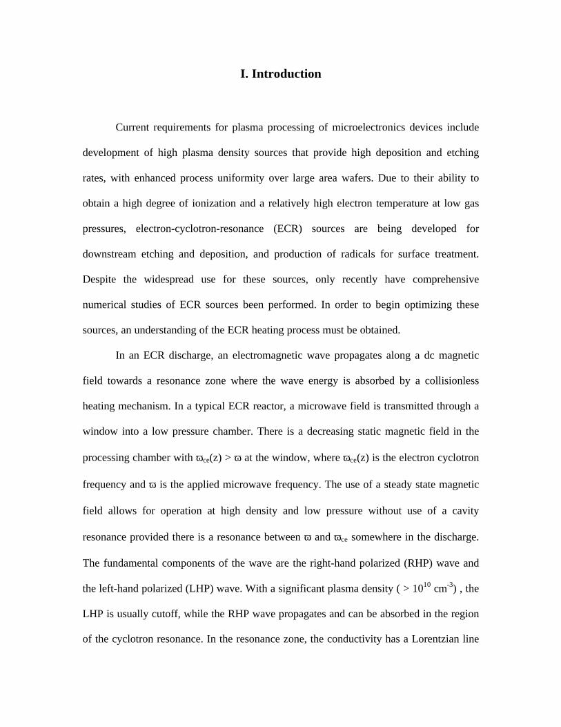
I. Introduction

Current requirements for plasma processing of microelectronics devices include

development of high plasma density sources that provide high deposition and etching

rates, with enhanced process uniformity over large area wafers. Due to their ability to

obtain a high degree of ionization and a relatively high electron temperature at low gas

pressures, electron-cyclotron-resonance (ECR) sources are being developed for

downstream etching and deposition, and production of radicals for surface treatment.

Despite the widespread use for these sources, only recently have comprehensive

numerical studies of ECR sources been performed. In order to begin optimizing these

sources, an understanding of the ECR heating process must be obtained.

In an ECR discharge, an electromagnetic wave propagates along a dc magnetic

field towards a resonance zone where the wave energy is absorbed by a collisionless

heating mechanism. In a typical ECR reactor, a microwave field is transmitted through a

window into a low pressure chamber. There is a decreasing static magnetic field in the

processing chamber with ωce(z) > ω at the window, where ωce(z) is the electron cyclotron

frequency and ω is the applied microwave frequency. The use of a steady state magnetic

field allows for operation at high density and low pressure without use of a cavity

resonance provided there is a resonance between ω and ωce somewhere in the discharge.

The fundamental components of the wave are the right-hand polarized (RHP) wave and

the left-hand polarized (LHP) wave. With a significant plasma density ( > 1010 cm-3) , the

LHP is usually cutoff, while the RHP wave propagates and can be absorbed in the region

of the cyclotron resonance. In the resonance zone, the conductivity has a Lorentzian line

shape with a full width at half maximum in the magnetic field corresponding to ∆ωce

equal to twice the electron collision frequency.1 This dependence on collision frequency

enables the efficient power transfer to the plasma at low pressures.

Efficient ECR coupling requires that the electron-neutral collision frequency be

much smaller than the electron cyclotron frequency. Under these operating conditions,

diffusion perpendicular to the magnetic field lines is reduced, thus reducing plasma losses

to the wall. However, due to enhanced confinement of electrons by the static magnetic

field lines, radial ionization profiles and charged particle densities tend to be strongly

nonuniform. Such non-uniformities in ionization profiles and charge particle distributions

will transfer to the ion fluxes reaching the substrate and eventually degrade flux

uniformity.

The spatial coupling of microwave radiation to the plasma in ECR systems is a

concern due to issues related to the uniformity of dissociation, electron heating, and

ultimately process uniformity. The uniformity of the ion flux at the substrate depends

strongly on the profile and location of the power deposition. Studies by Graves et al.2

suggest that uniform conditions at the substrate surface appear to require a power profile

peaked off-axis. Hidaka et al.3 obtained similar results. Their studies showed that ECR

plasma sources using a circular TE01 mode provide better uniformity over a larger area

than that produced by conventional TE11 mode microwaves.3 In the case of the TE11

mode, the electric field has a strong peak at the center of the waveguide. This may cause

the peaking of the plasma density at the central region, while the plasma density near the

sidewall decreases because of recombination of charged particles on the sidewall.4 On the

other hand, the TE01 mode has a peak off axis. This strong electric field near the wall may

compensate for recombination losses at the wall.

Considerable effort has been expended on numerical analysis and experimental

measurements of microwave propagation in ECR plasmas. Stevens and Checchi5

developed a predictive 1-D model by combining a simple plasma density model with a

ray tracing method to achieve a first approximation to the self-consistent ECR system.

Wu, Graves, and Kilgore6 studied the behavior of compact 2-D ECR plasma sources by

using a using a hybrid electron fluid particle ion and particle neutral model. In addition,

non-uniform depletion of neutral gas was examined by using a 2D Monte Carlo method.

Lieberman and Gottscho7 used a spatially averaged global model based on particle and

energy conservation to simulate ECR behavior.

In recent studies the finite-difference time-domain (FDTD) method has been used

to study the electromagnetic fields inside a compact ECR source. For example, Muta et

al.8 has investigated microwave propagation in ECR plasmas by using a FDTD method.

They performed one-dimensional simulations of the microwave propagation and

discussed the characteristics of wave propagation through comparisons with their

microwave ray tracing method measured by interferometry. Tan and Grotjohn9 solved for

electromagnetic fields inside an unmagnetized plasma-loaded microwave cavity reactor

using the FDTD method using three-dimensional cylindrical coordinates. The electrical

behavior of the discharge inside the reactor was modeled by solving the electron

momentum transport equation. More recently Gopinath and Grotjohn10 developed a

three-dimensional electromagnetic particle-in-cell (PIC) model to simulate a compact

ECR source. The FDTD technique was used to model the microwave fields. The PIC

technique was used to model the dynamics of both the electrons and the ions in the

plasma.

To investigate some of the previously discussed issues, a FDTD simulation for

microwave injection and propagation has been developed. The FDTD simulation was

incorporated as a module in the 2-dimensional Hybrid Plasma Equipment Model

(HPEM).11-13 Plasma dynamics are coupled to the electromagnetic fields through a tensor

form of Ohm’s law. The FDTD simulation uses a leap-frog scheme for time integration,

with time steps that are 30% of the Courant limit until reaching the steady state. Power

deposition calculated in the FDTD module is then used in solving the electron energy

equation.

1.2 References

1. M. A. Lieberman and A. J. Lichtenberg, Priciples of Plasma Discharges and Materials

Processing, John Wiley and Sons, Inc., New York, 1994.

2. D. B. Graves, H. Wu, and R. K. Porteous, Jpn. J. Appl. Phys., vol. 32, p. 2999, 1993.

3. R.Hidaka, T. Yamaguchi, N. Hirotsu, T. Ohshima, R. Koga, M. Tanaka, and Y.

Kawai, Jpn. J. Appl. Phys., vol. 32, p. 174, 1993.

4. H. Kim, Y. Tuchihashi, K. Matsuo, K. Muraoka, and M. Akazaki, T. IEEE Jpn., 109-

A, p. 149, 1989.

5. J. E. Stevens and J. L. Cecchi, Jpn. J. Appl. Phys., vol. 32, p. 3007, 1993.

6. H. Wu, D. B. Graves, M. Kilgore, Plasma Sources Sci. Technol., vol. 6, p. 231, 1997.

7. M. A. Lieberman and R. A. Gottscho, Physics of Thin Films, 1994.

8. H. Muta, T. Sakoda, Y. Ueda, and Y. Kawai, Jpn. J. Appl. Phys., vol. 36, p. 872,

1997.

9. W. Tan and T. A. Grotjohn, J. Vac. Sci. Technol. A, vol. 12, p. 1216, 1994.

10. V. P. Gopinath and T. A. Grothjohn, IEEE Transactions in Plasma Science, vol. 23,

p. 602, 1995.

11. P. L. G. Ventzek, M. Grapperhaus and M. J. Kushner, J. Vac. Sci. Technol. B, vol. 16,

p. 3118, 1994.

12. M. J. Grapperhaus and M. J. Kushner, J. Appl. Phys, vol. 81, p. 569, 1997.

13. S. Rauf and M. J. Kushner, J. Appl. Phys., vol. 81, p. 5966, 1997.

6

II. Model Description

2.1 Hybrid Plasma Equipment Model (HPEM)

The HPEM is a two-dimensional, plasma equipment model developed at the

University of Illinois.1-6 The HPEM has the capability of modeling complex reactor

geometries and wide variety of operating conditions. The HPEM allows for a variety of

plasma heating sources and gas chemistries. The base two-dimensional HPEM consists of

an electromagnetic module (EMM), an electron energy transport module (EETM) and a

fluid kinetics simulation (FKS). Electromagnetic fields and corresponding phases are

calculated in the EMM. Specifics on the EMM module will be discussed in Section 2.4

Electromagnetic fields calculated in the EMM are used in the EETM to generate electron

energy distribution functions as a function of position and phase. Methods on

determining the electron distribution function will be discussed in Section 2.2. The

electron distribution functions are used to generate sources for electron impact processes

and electron transport coefficients. Parameters determined in the EETM are transferred to

the FKS where momentum and continuity equations are solved for all heavy particles. A

drift diffusion formulation is used for electrons to enable an implicit solution of Poisson's

equation for the electric potential. The FKS solves for species densities and fluxes.

Details of the FKS module will be discussed in Section 2.3. The species densities and

electrostatic fields produced in the FKS are transferred to the EMCS and the EMM.

These modules are iterated until a converged solution is obtained. A flowchart of the

HPEM is shown in Figure 2.1. Note the HPEM has numerous other modules that are

described in greater detail elsewhere.1-6

7

2.2 The Electron-Energy Transport Module (EETM)

The EETM solves for electron impact sources and electron transport properties by

using electric and magnetic fields computed in the EMM and FKS. There are two

methods for determining these parameters. The first method determines the electron

temperature by solving the electron energy equation. The second method uses a Monte

Carlo simulation for electron transport to gather statistics used to generate the electron

energy distribution (eed) as a function of position.

The electron energy equation method first solves the zero order Boltzman

equation for a range of predetermined Townsend values to create a table that provides an

eed for each Townsend value. Once the eed isobtained, an average temperature, defined

as 3

2 <ε>, where <ε> is the average energy, is computed from the eed. Electron mobility,

thermal conductivity, energy loss rates due to collisions, and electron impact rate

coefficients are also determined from the eed’s.

With all these parameters known as a function of electron temperature, the

following steady state electron energy equation is solved,

( )∇ ∇ ∇ ⋅k T + T = P - Pe e heating lossΓ , (2.2.1)

where Te is the electron temperature, k is the thermal conductivity, Γ is the electron flux,

Pheating is the power deposition rate, and Ploss is the power loss to collisions. Equation

(2.2.1) is solved by successive over relaxation, with transport coefficients being updated

according to the local electron temperature.

8

The second method for determining electron transport properties is by the

Electron Monte Carlo Simulation (EMCS). The EMCS simulates electron trajectories

according to local electric and magnetic fields and collision processes. Initially the

electrons are given a Maxwellian distribution and randomly distributed in the reactor

weighted by the current electron density. Particle trajectories are computed using the

Lorentz equation,

( )Bx v + Em

q =

dt

vd

e

e , (2.2.2a)

anddr

dt = v , (2.2.2b)

where v, E, and B are the electron velocity, local electric field, and magnetic field

respectively. Equations (2.2.2) are updated using a second order predictor corrector

method. The electron energy range is divided into discrete energy bins. Within an energy

bin, the collision frequency, νi, is computed by summing all the possible collisions within

the energy range,

νε

σii

eijk j

j,k

2

m N=

∑

1

2

, (2.2.3)

where εi is the average energy within the bin, σijk is the cross section at energy i, for

species j and collision process k, and Nj is the number density of species j. The free-flight

time is randomly determined from the maximum collision frequency. After the free-

9

flight, the type of collision is determined by the energy of the pseudoparticle. The

corresponding energy bin in referenced and a collision is randomly selected from that

energy bin, with a null reaction making up the difference between the maximum and

actual collision frequency. At the end of the EMCS, the electron temperature, collision

frequency and electron impact rate coefficients are determined by convolving the electron

energy distribution function with the process cross section.

2.3 Fluid-Chemical Kinetics Simulation (FKS)

The FKS solves the fluid transport equations to provide species densities and

fluxes. The module also includes chemical reactions and a solution of Poisson’s equation

and/or an ambipolar field solution for the electric potential and time-dependent

electrostatic fields. Electron transport coefficients and electron impact rates needed to

solve the fluid and potential equations are obtained from the EETM. Ion and neutral

transport coefficients are obtained from a database or by using Lenard-Jones parameters.

The species densities are calculated from the continuity equation,

∂∂N

t = - + Si

i i∇ ⋅Γ , (2.3.1)

where Ni, Γi, and Si are the species density, flux, and source for species i. The flux for

each species can be determined by using a drift diffusion or a heavy body momentum

equation. Electron densities are determined using the drift diffusion formulation,

Γi i i i s i i = q N E - D Nµ ∇ , (2.3.2)

10

where µi is the mobility of species i, Di is the diffusion coefficient, qi is the species

charge in units of elementary charge, and Es is the electrostatic field. Heavy ion and

neutral fluxes can be determined by using the previous drift diffusion method or by using

the heavy body momentum equation,

( ) ( ) ( ) ijjijij ji

ji

i

iiiiii

i

i v - vNNm + m

m - EN

m

q + vv N - kTN

m

1- =

tν⋅∇∇

∂Γ∂

∑ , (2.3.3)

where Ti is the species temperature, vi is the species velocity given by Γi / Ni, and νij is

the collision frequency between species i and species j.

Solutions to Equations (2.3.2-2.3.3) requires knowledge of the local electrostatic

fields. Electrostatic fields can be determined in two ways. The first method solves

Poisson’s equation for the electric potential. Using the drift diffusion equation, (2.3.2), an

implicit form of Poisson’s is,

Γ∇⋅∇∆+ρ=

φ∇

µ∆+σ∆ε⋅∇ ∑ ∑∑ ∆+

i

tjj

tiii

tt t

i

2ii

2i q - NDqte - Nqte t - , (2.3.4)

where σ is the material conductivity and is nonzero only outside of the plasma region, e

is elemental charge, qi, µi, Ni, and Γi are the charge state, mobility, density, and the flux

of species i at time t, respectively; Γj is the flux for species j at time t, and φt + ∆t is the

electric potential at time t + ∆t. The summations over i are taken for those species using

the drift diffusion formulation and the summation over j is taken for those species using

11

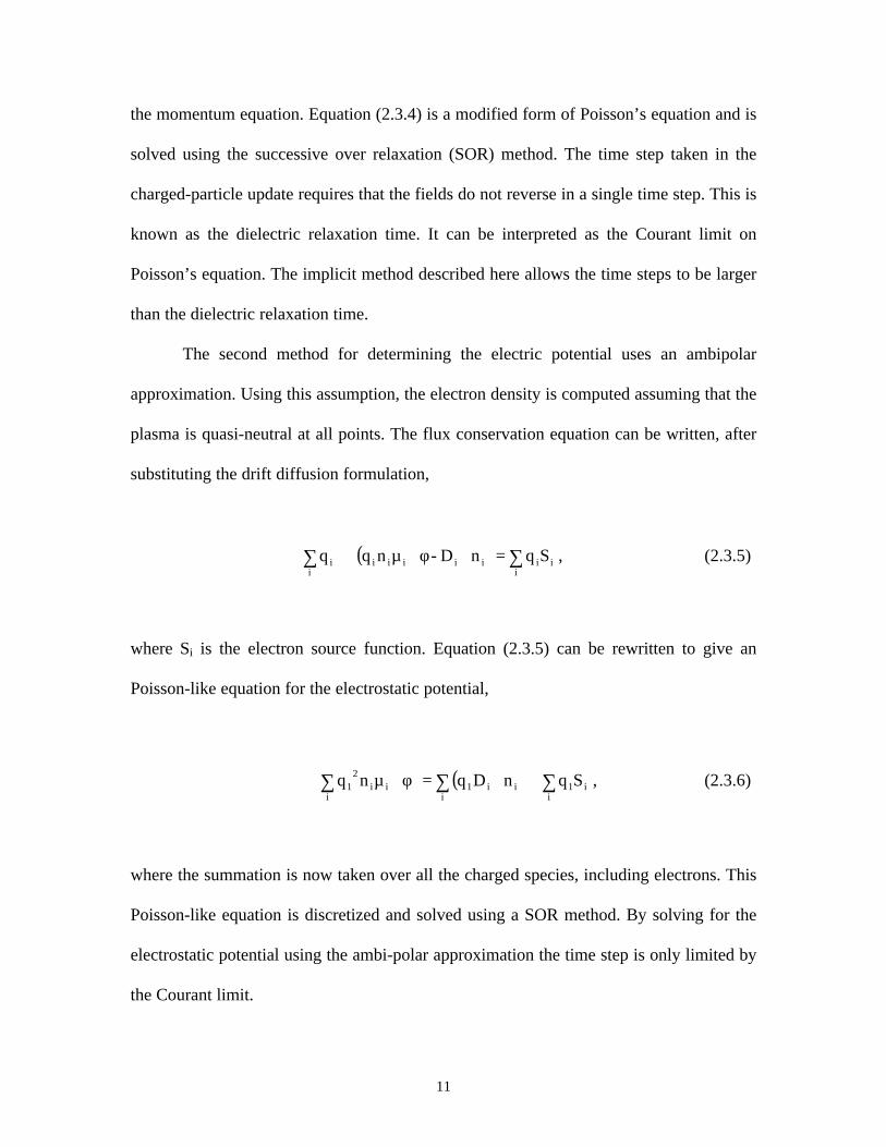
the momentum equation. Equation (2.3.4) is a modified form of Poisson’s equation and is

solved using the successive over relaxation (SOR) method. The time step taken in the

charged-particle update requires that the fields do not reverse in a single time step. This is

known as the dielectric relaxation time. It can be interpreted as the Courant limit on

Poisson’s equation. The implicit method described here allows the time steps to be larger

than the dielectric relaxation time.

The second method for determining the electric potential uses an ambipolar

approximation. Using this assumption, the electron density is computed assuming that the

plasma is quasi-neutral at all points. The flux conservation equation can be written, after

substituting the drift diffusion formulation,

( )∑ ∑=∇φ∇µ⋅∇i i

iiiiiiii Sq n D- nqq , (2.3.5)

where Si is the electron source function. Equation (2.3.5) can be rewritten to give an

Poisson-like equation for the electrostatic potential,

( ) ∑∑∑ +∇=

φ∇µ⋅∇

ii1

iii1

iii

21 Sq nDq nq , (2.3.6)

where the summation is now taken over all the charged species, including electrons. This

Poisson-like equation is discretized and solved using a SOR method. By solving for the

electrostatic potential using the ambi-polar approximation the time step is only limited by

the Courant limit.

12

2.4 The Electromagnetic Module (EMM)

In the current model developed here, the electromagnetic fields, E(r,z,φ) and

B(r,z,φ), are solved for in the entire volume of the reactor using a FDTD method starting

with the following forms of Maxwell’s equations,

∇ ×∂∂

E = - B

t, (2.4.1a)

∇ ×∂∂

H = J + D

t, (2.4.1b)

ρ⋅∇ = D . (2.4.1c)

Using the assumption of charge neutrality (ρ=0) and that the dielectric parameters

µ, σ, and ε are independent of time, we consider a 2-dimensional, cylindrical grid with

electromagnetic components of the following form,

E (r,z) = Eθ$θ , (2.4.2a)

B (r,z) = Br $r + Bz $z . (2.4.2b)

Substituting into Equations (2.4.1) the following system of equations are

obtained. These are equivalent to Maxwell’s equations in a cylindrical coordinate system

(r, θ, z),

∂∂

=∂∂

−∂∂

−E B Bθ

θµεσεt z r

r z1( )

| |E , (2.4.3a)

13

∂∂

=∂∂

B Er

t zθ

, (2.4.3b)

∂∂

= −∂

∂B Ez

t r

r

r

1 ( )θ. (2.4.3c)

In Equations (2.4.3), the following identities, ,E = J ⋅σ B = Hµ , and

D = Eε were used. The transverse electric fields (TE) used in the simulations have

0 Ek =⋅ , with components Eθ, Br, and Bz as previously shown. The spatial locations of

components of B and E may be chosen so as to provide centered spatial differencing.

The simulations performed here use an alternating direction implicit scheme with a 22

1

dimension alternating grid. Azimuthal electric fields are calculated at grid points, while

magnetic fields are calculated at locations shifted by half a grid cell, as shown in Figure

2.2.

The FDTD simulation uses a leap-frog scheme for time integration of Maxwell’s

equations. The electric fields are calculated at time t and the magnetic fields are

calculated at time t + ∆t/2. The finite differencing representation of Maxwell’s equations

is given by,

t t

2

t t

zzrr

tt t

j)(i,E -r

j),2

1-(i B- j),

2

1(iB

- z

)2

1-j(i, B- )

2

1j(i,B

1

t

j)(i, E- j)(i,E

∆+θ

∆+

θ∆+

θ

εσ

∆

+

∆

+

µε

=∆

, (2.4.4a)

14

z

j)(i, E- )1j(i,E

t

)2

1j(i, B- )

2

1j(i,B 2

t-t

r2

t t

r

∆+

=∆

++θθ

∆∆+

, (2.4.4b)

( )

r2

rj)r(i,

j)(i, Ej)r(i, - j)1,(i Ej)1,r(i

t

j),2

1(i B- j),

2

1(iB 2

t-t

z2

t t

z

∆

∆

+

++=

∆

++θθ

∆∆+

, (2.4.4c)

where r ,σ, µ, and ε are the radius, conductivity, permittivity and permeability of the

medium, respectively, at location (i, j) [Note: (i, j) corresponds to (r,z)]. ∆r and ∆z are the

grid sizes in the r- and z- directions and ∆t is the integration time step. The Courant

condition on the allowed time step for time integration is given by

t c

1

z

1

r

1 2

1-

22∆>

∆+

∆, (2.4.4)

where c is the speed of light in the medium.

The conduction current density, J , in the plasma is related to the electron drift

velocity, v , by,

J = q n ve , (2.4.5)

where ne is the plasma density. To obtain an expression for v , a first moment is formed

by multiplying the Boltzmann equation by v and integrating over velocity. Assuming a

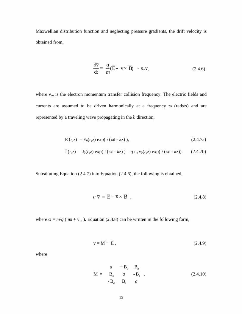
15

Maxwellian distribution function and neglecting pressure gradients, the drift velocity is

obtained from,

dv

dt E v B v = ×q

mm( + ) - ν , (2.4.6)

where νm is the electron momentum transfer collision frequency. The electric fields and

currents are assumed to be driven harmonically at a frequency ω (rads/s) and are

represented by a traveling wave propagating in the $z direction,

E (r,z) = E0(r,z) exp( i (ωt - kz) ), (2.4.7a)

J (r,z) = J0(r,z) exp( i (ωt - kz) ) = q ne v0(r,z) exp( i (ωt - kz)). (2.4.7b)

Substituting Equation (2.4.7) into Equation (2.4.6), the following is obtained,

α v E v B= ×+ , (2.4.8)

where α = m/q ( iω + νm ). Equation (2.4.8) can be written in the following form,

E M = v -1 ⋅ , (2.4.9)

where

M

B B

B - B

- B B

z

z r

r

=

αα

α

θ

θ

−

. (2.4.10)

16

Combining Equation (2.4.9) with Equation (2.4.5), a tensor form of Ohm’s law is

obtained,

E = E M n q = v n q = J -1ee ⋅σ⋅ . (2.4.11)

Since Bθ, Er, and Ez are zero, equation (2.4.11) can be expanded as,

( )( )

( )

+ααααα

α+α

++αα=

θθ

0

E

0

B B-BB

BB-

BBB B

B B

n q

J

J

J

2z

2rzr

r2

z

zrz2

r2

2z

2r

2

e

z

r

. (2.4.12)

The azimuthal conduction current density, Jθ, is,

θθ ααα

E ) B+ B+ (

n q = J 2

2z

2r

2

e . (2.4.13)

To incorporate Jθ into Maxwell’s equations, only the real component is

considered. This is justified by the fact that Maxwell’s equations represent real,

instantaneous fields. If an electric field is used to excite a gas discharge or to heat the

electrons, then the energy absorbed is proportional to the real part of the conductivity.

The real component of Equation (2.4.13) is,

17

[ ]Re J =

1 + +

1 + -

+ 2

q n

m E

2cyc

m

cyc2

m m

2e

e mθ θ

ω ω

ν

ω ω

νω

ν

ν

2

2

2

2

2 2

, (2.4.14)

where ωcyc = q |Btot| / me, is the magnitude of the cyclotron frequency. This equation is

identical to that presented by Cherrington.7 If the collision frequency is reasonably small

with respect to the frequency of the electromagnetic field (νm2 << ω2) and if the

electromagnetic frequency approaches the cyclotron frequency, then

[ ]Re q n

2 m

1

+ ( - )

2e m

e m cyc2σ

νν ω ω⊥ ≈

2 . (2.415)

If ω = ωcyc the conductivity peaks in a resonant manner and exhibits a Lorentzian

line shape with a full width at half maximum of 2νm. The peak in the conductivity can be

understood as the condition under which the motion of the electron in the magnetic field

is synchronous with the driving electromagnetic field, setting up a condition under which

the electron continuously gains energy from the electric field. This is analogous to the

conditions achieved in a steady state electric field where the velocity of the electrons (or

the current) is impeded by collisions (Re[σ] ~ 1/νm). Hence, collisions limit the amount

of energy absorbed by electrons, but transfer electron energy to the neutral gas. The

absorption of the microwave energy is by both ions and electrons. However, since work

the done on a charged particle by an electric field varies inversely as the particle mass,

the energy imparted to an electron is significantly greater than the energy imparted to an

18

ion. Therefore, direct energy transfer from the incident electric fields to the ions can be

neglected here. Transfer of the electromagnetic energy to the neutral gas takes place

through Joule (elastic and inelastic heating) following electron cyclotron heating of the

electron gas.

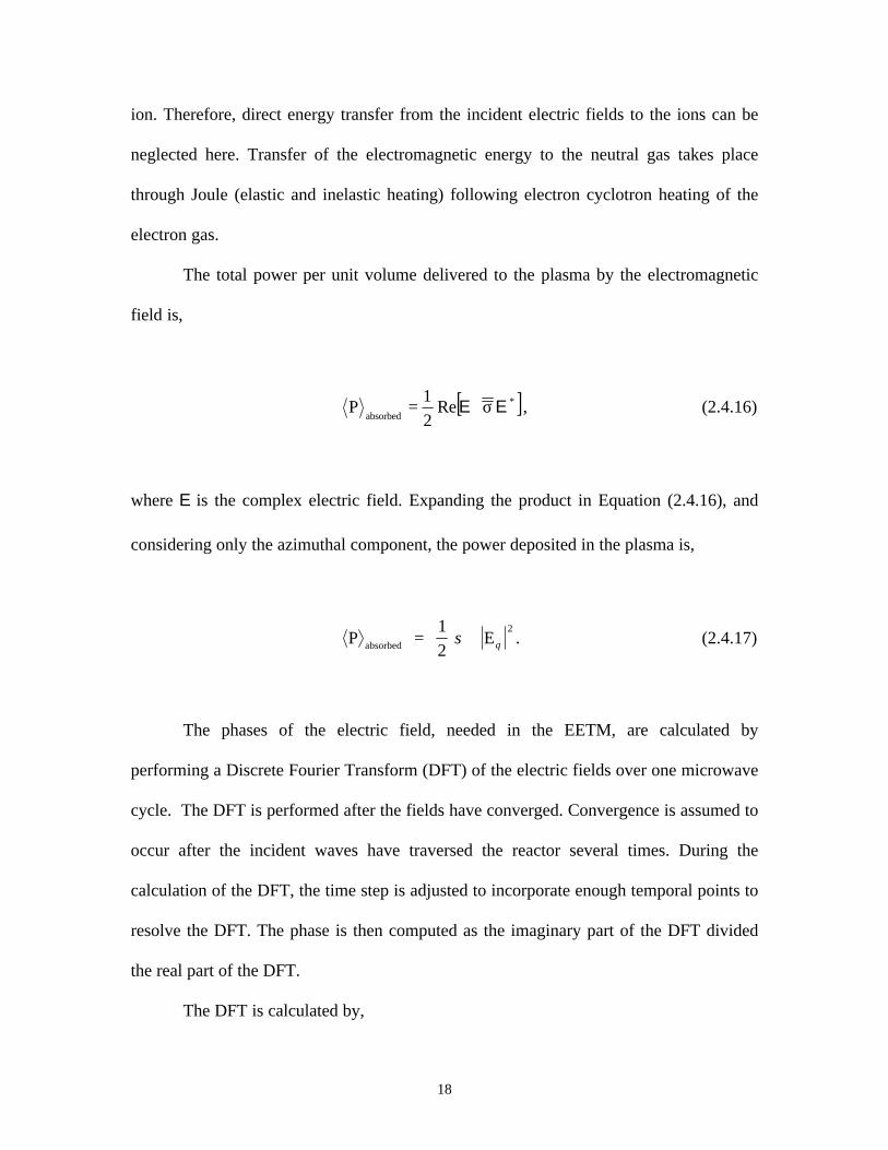
The total power per unit volume delivered to the plasma by the electromagnetic

field is,

[ ]*

absorbed Re

2

1 = P EE σ⋅ , (2.4.16)

where E is the complex electric field. Expanding the product in Equation (2.4.16), and

considering only the azimuthal component, the power deposited in the plasma is,

P = 1

2 Eabsorbed σ θ⊥

2. (2.4.17)

The phases of the electric field, needed in the EETM, are calculated by

performing a Discrete Fourier Transform (DFT) of the electric fields over one microwave

cycle. The DFT is performed after the fields have converged. Convergence is assumed to

occur after the incident waves have traversed the reactor several times. During the

calculation of the DFT, the time step is adjusted to incorporate enough temporal points to

resolve the DFT. The phase is then computed as the imaginary part of the DFT divided

the real part of the DFT.

The DFT is calculated by,

19

∑=

π

θ=1-N

0n

knN

2j-

e (n)E (k)E , (2.4.18)

where E(k) is the DFT of the electric field, k is the harmonic number, and N is an

appropriately large integer to achieve proper temporal resolution. For these simulations

the fundamental harmonic, k = 1, was used along with N = 100 temporal points. The

phase was then calculated as,

[ ][ ]1) k j,(i, Re

1)k j,(i,Im j)(i,

==

=φEE

, (2.4.19)

where Im[E(i,jk=1)] and Re[E(i,jk=1)] are the imaginary and real parts of the DFT,

respectively.

When time domain electromagnetic fields are obtained using finite difference

techniques in an unbounded space, there must ultimately be a method of limiting the

domain in which the field is computed. This is achieved here by truncating the mesh and

using absorbing boundary conditions at those artificial boundaries which simulates the

unbounded space. Due to the nature of the 22

1 dimension alternating direction implicit

scheme, boundary conditions which use constant gradients for electromagnetic fields

cause spurious reflections of the incident waves. To remove these unwanted reflections

back into the waveguide a linearized first order wave equation was imposed as a

boundary condition to simulate empty space,

20

∂

∂+

∂∂

=∂

∂+

∂∂ θθθ

+θ

t

1)-(jE

t

j)(i,E

c

1

z

E

z

E n1n

. (2.4.20)

In these simulations, the system of interest uses circular TE(0,n) microwave mode

fields injected along the axis of a cylindrically symmetric downstream reactor to excite

the plasma. The complex electric and magnetic field components for circular TE mode

waves as,

( ) ( ) ( )[ ] z)exp(-jm D mCrJ'A r22rmr

mn βφ+φβε

β=θ sincosE , (2.4.21a)

( ) ( ) ( )[ ] z)exp(-jm D mCrJ'A- r22rmrz

mn βφ+φβωµε

ββ=ρ sincosH

, (2.4.21b)

( ) ( ) ( )[ ] z)exp(-jm D mCrJA j - r22rm

2r

mnz βφ+φβωµεβ

= sincosH , (2.4.21c)

where Eθ, Hr, and Hz, are the complex azimuthal electric field, radial magnetic field

intensity, and axial magnetic field intensity, respectively, and J(βrr) and J’(βrr) are the

Bessel functions and their derivatives.8 Likewise βr is defined as,

a

'mnr

χ=β , (2.4.22)

where χ’mn is the zeroes of J’(βra) and a is the radius of the waveguide.

21

In this work, m = 0 and z = 0. The instantaneous field vectors are given by the real

part of the product of the complex field and the time harmonic variation e-jωt. Incident

waves having these amplitudes were introduced as a boundary condition on a dielectric

window. These fields produce electric field distributions which are zero on the axis of

symmetry and the metallic edges of the waveguide, and have a peak off axis. The number

of nodes between the axis of symmetry and the waveguide edge will vary accordingly to

the mode of excitation. Typical electric fields are shown in Figure 2.3 for modes n = 1

and n = 2.

The effects of absorbing boundary conditions are shown in Figure 2.4. A circular

transverse electric TE(0,1) field mode, operating at 3.0 GHz, was injectedat the top (z=50

cm) of a metallic waveguide and propagates towards the bottom (z=0 cm) of the open

ended waveguide. In case (a), a constant electric field gradient boundary condition was

imposed at the bottom of the waveguide. As the electromagnetic wave reached the lower

boundary, the imposed boundary condition pinned the electromagnetic field at zero

thereby causing a spurious reflection of the incident wave. The reflected wave combined

with the incident wave to create a standing wave pattern, as can be seen in Figure 2.4. In

case (b), a linearized first order wave equation was imposed as a boundary condition to

simulate unbounded surroundings. In this case, spurious reflections of the incident wave

were removed.

22

2.6 References

1. P. L. G. Ventzek, R. J. Hoekstra and M. J. Kushner, J. Vac. Sci. Technol. B, vol. 12,

p. 416, 1993.

2. P. L. G. Ventzek, M. Grapperhaus and M. J. Kushner, J. Vac. Sci. Technol. B, vol. 16,

p. 3118, 1994.

3. W. Z. Collison and M. J. Kushner, Appl. Phys. Lett., vol. 68, p. 903, 1996.

4. M. J. Kushner, W. Z. Collison, M. J. Grapperhaus, J. P. Holland and M. S. Barnes, J.

Appl. Phys., vol. 80, p. 1337, 1996.

5. M. J. Grapperhaus and M. J. Kushner, J. Appl. Phys, vol. 81, p. 569, 1997.

6. S. Rauf and M. J. Kushner, J. Appl. Phys., vol. 81, p. 5966, 1997.

7. B. E. Cherrington, Gaseous Electronics and Gas Lasers, Pergamon Press, New York,

1979.

8. C. A. Balanis, Advanced Engineering Electromagnetics, John Wiley & Sons, New

York, 1989.

23

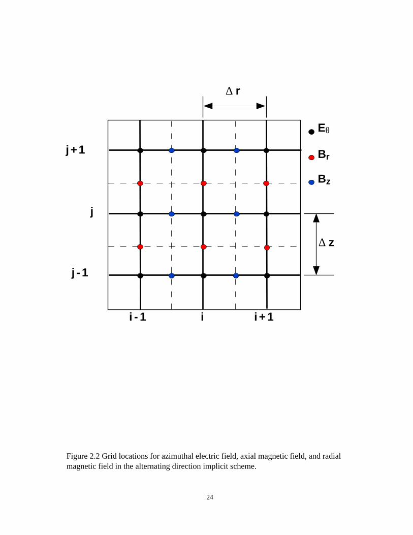
Figure 2.2 Grid locations for azimuthal electric field, axial magnetic field, and radial magnetic field in the alternating direction implicit scheme.

24

i - 1 i i + 1

j + 1

j

j - 1

Eθ

Br

Bz

∆ r

∆ z

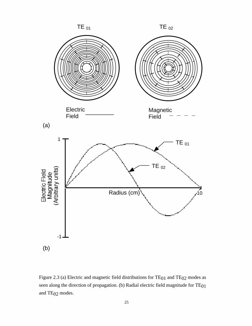
Figure 2.3 (a) Electric and magnetic field distributions for TE01 and TE02 modes as

seen along the direction of propagation. (b) Radial electric field magnitude for TE01

and TE02 modes.

25

TE 01 TE 02

ElectricField

MagneticField

Radius (cm) 10

1

-1

(a)

(b)

TE 01

TE 02

Figure 2.4 Azimuthal electric, radial magnetic, and axial magnetic fields for varying bottom boundary conditions. Results for (a) constant electric field gradient (b) a linearized first order wave equation boundary condition at the bottom of the waveguide are shown.

26

1 0

Arbitrary Units

a)

b)

Electric Field Radial Magnetic Field Axial Magnetic Field

Electric Field Radial Magnetic Field Axial Magnetic Field

Radius (cm)0

50

10

0

27

III. Consequences of Mode Structure, Magnetic Field

Configuration, and Operating Conditions on ECR Plasma Parameters

3.1 Simulated Reactor Geometry, Operating Conditions, and Base Case Analysis.

The ECR model simulates a cylindrical reactor shown in Figure 3.1. Gases are

injected into the reactor through a ring nozzle located near the microwave window and

are exhausted downstream through a pump port. Nitrogen is used as the feedstock gas.

Gas pressure was varied from 0.5 – 50 mTorr and flow rates were varied from 5 – 20

sccm resulting in residence times of a few milli-seconds. Typical operating power ranged

from 500 – 1500 W. The collisional processes for neutral particles and ions were, (1)

ionization, excitation, and momentum transfer collisions between electrons and neutral

particles, (2) Coulomb collisions between electrons and ions, (3) charge exchange

collisions between ions and neutral particles, and (4) momentum transfer collisions

among neutral particles. The full reaction scheme is listed in Table 3.1. Electron impact

reactions with molecular nitrogen include excitation up to the eighth vibrational state and

the third electronic state of N2. The vibrational and electronic states used in the model are

the sum of all the vibrational and electronic states created by electron impact collisions,

respectively.

Excitation of the electron gas occurs through ECR coupling of the incident

microwave field in the presence of the magnetic field produced by the coils surrounding

the throat region of the chamber. Transverse electric microwave fields, TE(0,n),

operating at 2.00 GHz, were used to sustain the plasma. Although in commercial reactors

a 2.45 GHz microwave is frequently used, a lower frequency was used in these

28

simulations to reduce the computation time. For proper computation of wave

propagation, a minimum number of grid points are needed. The grid resolution for in the

direction of propagation must be at least 80 grid points per wavelength. Resolution in the

direction perpendicular to propagation can be coarser, with about 40 grid points per

wavelength. The grid dimensions used here were 160 points in the axial direction and 55

points in the radial direction, for a total of 8,800. Applying the previous criterion, the

total number of points needed for the same geometry operating at 2.45 GHz is 12,740. By

using a frequency of 2.00 GHz, the cpu time is reduced by 33%, while the results

obtained at the lower frequency are comparable to those obtained at 2.45 GHz.

i) Plasma Parameters

The base case was N2 at 1 mTorr, 10 sccm and 750 W. The circularly transverse

electric fields are injected at the top of the reactor through a waveguide antenna. The

wave propagates through the dielectric window and into the processing chamber. A static

magnetic field is generated by a direct current solenoid, designed to produce a resonance

zone in the throat of the chamber. Magnetic field lines and contours are shown in Figure

3.2. The top set of magnetic coils are use to determine the location of resonance, while

the bottom coil is used to enhance confinement of charged species and allow tailoring of

the flux profile to the wafer surface. Base case simulations used only the upper most top

coil and the subcoil. For the given geometry and operating conditions, the primary

resonance occurs in the upper region of the reactor where B = 714 Gauss. There is also a

secondary resonance located downstream that occurs when the subcoil is used. When ωcyc

= ω, the conductivity peaks in a resonant manner and exhibits a Lorentzian line shape, as

29

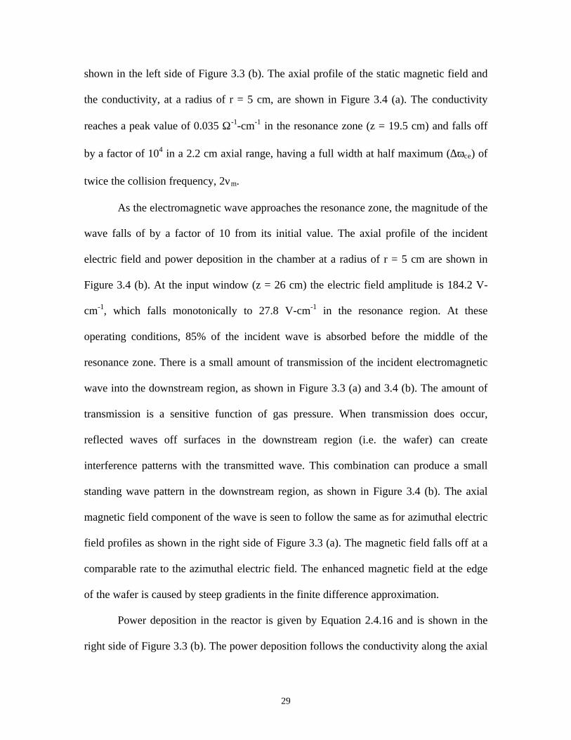
shown in the left side of Figure 3.3 (b). The axial profile of the static magnetic field and

the conductivity, at a radius of r = 5 cm, are shown in Figure 3.4 (a). The conductivity

reaches a peak value of 0.035 Ω-1-cm-1 in the resonance zone (z = 19.5 cm) and falls off

by a factor of 104 in a 2.2 cm axial range, having a full width at half maximum (∆ωce) of

twice the collision frequency, 2νm.

As the electromagnetic wave approaches the resonance zone, the magnitude of the

wave falls of by a factor of 10 from its initial value. The axial profile of the incident

electric field and power deposition in the chamber at a radius of r = 5 cm are shown in

Figure 3.4 (b). At the input window (z = 26 cm) the electric field amplitude is 184.2 V-

cm-1, which falls monotonically to 27.8 V-cm-1 in the resonance region. At these

operating conditions, 85% of the incident wave is absorbed before the middle of the

resonance zone. There is a small amount of transmission of the incident electromagnetic

wave into the downstream region, as shown in Figure 3.3 (a) and 3.4 (b). The amount of

transmission is a sensitive function of gas pressure. When transmission does occur,

reflected waves off surfaces in the downstream region (i.e. the wafer) can create

interference patterns with the transmitted wave. This combination can produce a small

standing wave pattern in the downstream region, as shown in Figure 3.4 (b). The axial

magnetic field component of the wave is seen to follow the same as for azimuthal electric

field profiles as shown in the right side of Figure 3.3 (a). The magnetic field falls off at a

comparable rate to the azimuthal electric field. The enhanced magnetic field at the edge

of the wafer is caused by steep gradients in the finite difference approximation.

Power deposition in the reactor is given by Equation 2.4.16 and is shown in the

right side of Figure 3.3 (b). The power deposition follows the conductivity along the axial

30

direction, exhibiting a Lorenztian line shape, while it reflects the profile of the azimuthal

electric field component along the radial direction. Power deposition occurs

predominantly within 3% of the resonance zone, although a small amount of power

deposition occurs near the bottom coil due to the second resonance region created by the

subcoil. Peak values of power deposition are 15.2 W-cm-3 in the resonance region and fall

off by a factor of 104 in a 2.6 cm axial distance downstream. In the upstream region, the

continual absorption of the incident electromagnetic wave produces a small amount of

power deposition that constitutes about 2% of the total.

Electron temperatures in ECR sources are typically higher than those obtained

using inductively coupled plasma (ICP) devices.1 Electron temperatures can exceed 8 eV

for pressures below 0.5 mTorr. Electron temperatures in the resonance region reflect

radial power deposition distributions, and have a peak value of 7.1 eV, as shown in the

left side of Figure 3.5 (a). In the steady state, the plasma generation by ionization of

neutrals is in balance with plasma losses due to diffusion. The solenoidal magnetic field

minimizes diffusion losses to the chamber walls. Diffusion therefore mainly occurs along

the magnetic field lines thereby allowing the radial electron temperature distribution to

maintain its profile far into the downstream region.

Due to a large electron mobility along the magnetic field lines, electrons initially

quickly transport out of the system, leaving ions behind and building a space charge

potential. This condition leads to ambi-polar diffusion of ions and the production of a

electropositive plasma. The high electron temperatures tend to produce a large electric

potential which has a uniform profile throughout the processing chamber, as shown in the

right side of Figure 3.5 (a).

31

ii) Gas dynamics

The ionization rates and electron densities are shown in Figure 3.6 (a). The

ionization rate has a maximum off axis near the peak in the electron temperature. The

peak value of the ionization rate in the resonance zone is 1.07 × 1016 cm-3-sec-1 and the

off axis distribution is maintained downstream. This distribution results from the

enhanced transport of hot electrons along the magnetic field lines which allows for

ionization to occur downstream. The electron density peaks in the resonance zone with a

value of 1.58 × 1011 cm-3. For these operating conditions, the radial distribution of

densities tend to reflect their radial sources, due to the strong radial confinement of

electrons by the magnetic field which enable the off axis distribution to be maintained

downstream. Due to the small amount of power deposition that occurs near the subcoil,

there is a local peak in the electron density. It will be shown in Section 3.5 that the

electron density is a sensitive function of pressure.

The distribution of N2(Χ 1Σg+) and its source are shown in Figure 3.6 (b). The

depletion of N2 occurs primarily by electron impact reactions. Therefore the gas density

has a minimum in the off axis region were the ion density peaks. However, production of

N2 is dominated by recombination at the walls and is strongest at the dielectric window,

were the density of excited species is the highest. The vector arrows shown in Figure 3.8

represent gas flow in the reactor chamber.

The N2(Χ 1Σg+, v=1) density and its source are shown in Figure 3.7 (a). Depletion

of the vibrational state occurs through electron impact reactions which produce the

electronic state N2(A 3Σu+). These reactions occur at high electron temperatures since the

threshold energy is ~ 6 eV. Therefore, the N2(Χ 1Σg+ v=1) production rate is negative and

32

follows the off axis peak in the ionization. In the volume beyond the radius of the

substrate the electron temperature decreases to the point where excitation to the first

electronic state is not important, thereby reducing losses enabling the production rate to

peak. The density of N2(Χ 1Σg+, v=1) reflects the off axis sink in the production rate.

The N2(A 3Σu+) density and source are shown in Figure 3.7 (b). The electronic

state is primarily produced through electron impact reactions with the ground state, N2(Χ

1Σg+) and the first vibrational state, N2(Χ 1Σg

+ v=1). Results suggest that excitation from

the ground state to the electronic state is in large part achieved through a vibrational

transition. The spatial distribution of excitation of N2(A 3Σu+) production follows that for

ionization and is peaked off axis. However, there is also a local peak in the production

rate near the dielectric window. This is due to a small peak in the density of the

vibrational state that occurs near the window. In this region, electron temperatures are

high enough to produce excitation from N2(Χ 1Σg+ v=1) to N2(A 3Σu

+). Steep gradients in

the radial direction suggest that the electronic state is short lived and its density depends

largely on local reaction kinetics.

The production of ground state atomic nitrogen, N(4S0), occurs dominantly

through the dissociation of ground state molecular nitrogen, N2(Χ 1Σg+). Density and

sources for N(4S0) are shown in Figure 3.8 (a). Production is peaked off axis and reflects

electron densities. Atomic nitrogen densities are uniform throughout the reactor, but

exhibit peaks at the walls surface from the quenching of N(2D0) and neutralization of

N+(3P). Density and sources for the N(2D0) state are shown in Figure 3.8 (b). The radial

gradients of N(2D0), suggest that it has a short lifetime and that densities largely depend

on local reaction kinetics, similar to N2(A 3Σu+).

33

Density and ionization rates for charged species N2+(Χ 2Σg

+) and N+(3P) are

shown in Figure 3.9. Production of N2+(Χ 2Σg

+) occurs predominately through an electron

impact collision with N2(Χ 1Σg+), while the production of N+(3P) occurs predominately

through a charge exchange collision with N2+(Χ 2Σg

+). Both charged species have

production and density peaks off axis. However, N2+(Χ 2Σg

+) retains its off axis peak

further downstream than N+(3P) because the diffusion perpendicular to the magnetic field

lines is smaller for the heavier N2+(Χ 2Σg

+) ion than the N+(3P) ion.

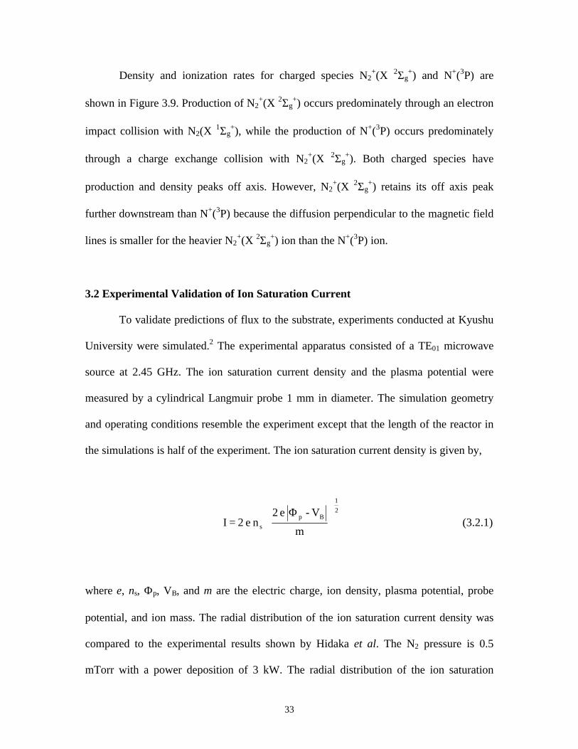
3.2 Experimental Validation of Ion Saturation Current

To validate predictions of flux to the substrate, experiments conducted at Kyushu

University were simulated.2 The experimental apparatus consisted of a TE01 microwave

source at 2.45 GHz. The ion saturation current density and the plasma potential were

measured by a cylindrical Langmuir probe 1 mm in diameter. The simulation geometry

and operating conditions resemble the experiment except that the length of the reactor in

the simulations is half of the experiment. The ion saturation current density is given by,

2

1

Bp

s m

V - e 2 n e 2 I

Φ= (3.2.1)

where e, ns, Φp, VB, and m are the electric charge, ion density, plasma potential, probe

potential, and ion mass. The radial distribution of the ion saturation current density was

compared to the experimental results shown by Hidaka et al. The N2 pressure is 0.5

mTorr with a power deposition of 3 kW. The radial distribution of the ion saturation

34

current density for both experiment and computation are in good agreement, as shown in

Figure 3.10. The radial ion saturation current density in the case of the TE01 mode is

uniform within 5% over an 8 inch diameter. Since the saturation current was obtained

from the plasma potential, such uniformity might have been expected from the uniformity

of the plasma potential distribution shown in the right side of Figure 3.5 (a). The

dependence of ion saturation current density on input microwave power is shown in

Figure 3.11. Theoretical predictions follow experimental trends with the saturation

current increasing linearly in proportion to microwave power.

3.3 Activation of Subcoil

Base case simulations were conducted with the magnetic subcoil activated.

Results based on parametric studies conducted with and without activation of subcoil are

discussed in this section. Magnetic field line configurations without and with activation

of the subcoil are shown in Figure 3.12. The bottom coil is used to enhance confinement

of charged species. By producing a solenoidal magnetic field configuration, diffusion

losses to the walls are significantly reduced. The average reactor electron density as a

function of power with and without activation of the subcoil is shown in Figure 3.13. The

electron density is higher with the subcoil than without. The electron density did increase

with increasing power without the subcoil but the slope is smaller than with the coil. At a

power of 500 W, the electron density is increased by 100% when operating with the

subcoil as compared to operating without the subcoil. At a power level of 1500 W, the

electron density is increased by more than 230%. This apparent saturation of the absorbed

power is qualitatively similar to measurements made in other systems using probes3 and

35

interferometry.4 This effect has been attributed to a failure of the microwaves to

propagate in an overdense plasma.5

The effects of activating the subcoil on electron temperature as a function of

power are shown in Figure 3.14. A larger electron temperature is obtained without

activation of the subcoil. The decrease in average electron temperature with the subcoil is

due to reduced diffusion losses. Ionization efficiency of the neutral gas is also enhanced

with the subcoil, as shown in Figure 3.15. The reactor average ion to neutral density ratio

follows the same dependence as the electron density. These results suggest that the

electron density may not be limited by the apparent saturation of absorbed power, as

previously mentioned, but instead may be limited by the diffusion losses.

Another benefit using the subcoil is to allow tailoring of the ion fluxes to the

wafer surface. The solenoidal magnetic field configuration causes the plasma density to

maintain the radial profile it had in the resonance zone near the substrate surface. The

effects of subcoil activation on the ion flux to the substrate are shown in Figure 3.16. The

increase in ion flux with increase in power reflects the overall increase in the reactor

average plasma density.

Flux uniformity is defined as,

Flux uniformity = Average

AveragePeak - - 1

Φ

ΦΦ, (3.3.1)

where ΦPeak and ΦAverage are the peak and average ion flux, respectively. The ion flux

profiles with and without activation of the subcoil are different at of 1 mTorr. Without

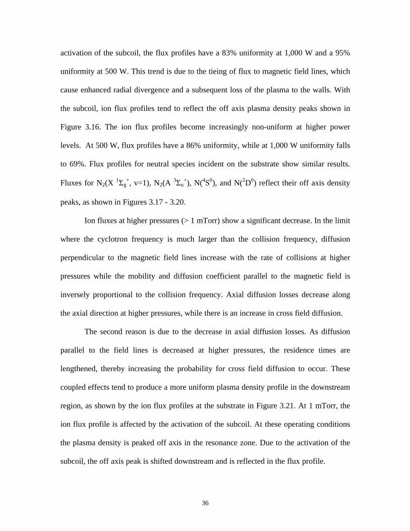
36

activation of the subcoil, the flux profiles have a 83% uniformity at 1,000 W and a 95%

uniformity at 500 W. This trend is due to the tieing of flux to magnetic field lines, which

cause enhanced radial divergence and a subsequent loss of the plasma to the walls. With

the subcoil, ion flux profiles tend to reflect the off axis plasma density peaks shown in

Figure 3.16. The ion flux profiles become increasingly non-uniform at higher power

levels. At 500 W, flux profiles have a 86% uniformity, while at 1,000 W uniformity falls

to 69%. Flux profiles for neutral species incident on the substrate show similar results.

Fluxes for N2(Χ 1Σg+, v=1), N2(A 3Σu

+), N(4S0), and N(2D0) reflect their off axis density

peaks, as shown in Figures 3.17 - 3.20.

Ion fluxes at higher pressures (> 1 mTorr) show a significant decrease. In the limit

where the cyclotron frequency is much larger than the collision frequency, diffusion

perpendicular to the magnetic field lines increase with the rate of collisions at higher

pressures while the mobility and diffusion coefficient parallel to the magnetic field is

inversely proportional to the collision frequency. Axial diffusion losses decrease along

the axial direction at higher pressures, while there is an increase in cross field diffusion.

The second reason is due to the decrease in axial diffusion losses. As diffusion

parallel to the field lines is decreased at higher pressures, the residence times are

lengthened, thereby increasing the probability for cross field diffusion to occur. These

coupled effects tend to produce a more uniform plasma density profile in the downstream

region, as shown by the ion flux profiles at the substrate in Figure 3.21. At 1 mTorr, the

ion flux profile is affected by the activation of the subcoil. At these operating conditions

the plasma density is peaked off axis in the resonance zone. Due to the activation of the

subcoil, the off axis peak is shifted downstream and is reflected in the flux profile.

37

As the pressure is increased, with the subcoil on, the magnitude of the flux

decreases. However, the uniformity of the flux profile is improved because the plasma

density profile has become more uniform in the downstream region. Flux magnitudes for

N2(Χ 1Σg+, v=1) and N(2D0) increase with increasing pressure, as shown in Figure 3.22

and 3.23. Subcoil activation tends to increase the fluxes because of an increased in the

rate of electron impact processes. The uniformity of the flux of these longed lived

neutrals do not have a strong dependence on subcoil activation, but instead are sensitive

to increased pressure gradients at the substrate surface that are at higher pressures.

However, the uniformity of the flux for N2(A 3Σu+), shown in Figure 3.24, is strongly

dependent on subcoil activation implying that the flux is sensitive to chemical kinetics

close to the substrate. The flux for ground state atomic nitrogen, shown in Figure 3.25

had little dependence on subcoil activation, at higher pressures, and had uniformity above

95%.

Overall, these results suggest that use of the subcoil causes the flux to the

substrate to more closely reflect the reactor density profiles. An increase in power leads

to the enhancement of any non-uniformities present in the flux profile. At higher

pressures the sensitivity on subcoil activation is decreased and the uniformity of the flux

is improved.

3.4 Results for Varying Modal Structures

Higher order circular TEon modes have several off axis peaks in the electric field

depending on the harmonic used. The use of higher order modes is believed to create

several off axis power deposition peaks and thereby provide greater uniformity at the

38

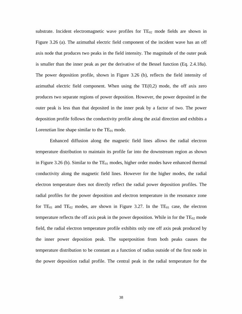
substrate. Incident electromagnetic wave profiles for TE02 mode fields are shown in

Figure 3.26 (a). The azimuthal electric field component of the incident wave has an off

axis node that produces two peaks in the field intensity. The magnitude of the outer peak

is smaller than the inner peak as per the derivative of the Bessel function (Eq. 2.4.18a).

The power deposition profile, shown in Figure 3.26 (b), reflects the field intensity of

azimuthal electric field component. When using the TE(0,2) mode, the off axis zero

produces two separate regions of power deposition. However, the power deposited in the

outer peak is less than that deposited in the inner peak by a factor of two. The power

deposition profile follows the conductivity profile along the axial direction and exhibits a

Lorenztian line shape similar to the TE01 mode.

Enhanced diffusion along the magnetic field lines allows the radial electron

temperature distribution to maintain its profile far into the downstream region as shown

in Figure 3.26 (b). Similar to the TE01 modes, higher order modes have enhanced thermal

conductivity along the magnetic field lines. However for the higher modes, the radial

electron temperature does not directly reflect the radial power deposition profiles. The

radial profiles for the power deposition and electron temperature in the resonance zone

for TE01 and TE02 modes, are shown in Figure 3.27. In the TE01 case, the electron

temperature reflects the off axis peak in the power deposition. While in for the TE02 mode

field, the radial electron temperature profile exhibits only one off axis peak produced by

the inner power deposition peak. The superposition from both peaks causes the

temperature distribution to be constant as a function of radius outside of the first node in

the power deposition radial profile. The central peak in the radial temperature for the

39

TE02 case produces ionization rate distributions that are peaked closer to the axis of

symmetry than those produced for the TE01 case, as shown in Figure 3.28.

The electron temperatures as a function of power for the TE01 and TE02 modes are

shown Figure 3.29. In the resonance zone, electron temperatures tend to be higher for

higher electric field modes. For the TE02 mode, the superposition of two power

deposition peaks produces higher temperature distributions than those produced by the

TE01 mode. Likewise in the resonance zone, electron densities tend to be higher for the

higher modes. Since the electron temperature is higher in this region, local ionization

rates will tend to be higher for the higher order modes, producing an increase in the local

value of the electron density. However, reactor averaged electron production rates are

higher for the lower modes because of lower diffusion losses that occur at the lower

temperature. This produces a higher reactor average plasma density for the TE01 mode

than the TE02 mode, as shown in Figure 3.30. In addition, the reactor average electron

temperature, shown in Figure 3.29 is lower for the TE01 mode. Such a decrease in the

reactor average electron temperature for the lower TE01 mode is due to reduced diffusion

losses and the cooling of the electron gas due to elastic collisions that occurs at the higher

densities. Subsequently, the ion to neutral density ratio is higher for the lower mode

structure. As shown in Figure 3.31, the TE01 mode structure is more efficient in the

overall ionization of the gas.

Ion flux profiles tend to reflect the off axis peaks in ionization rates and plasma

densities. The ion flux shows the effect of the inner peak in the power deposition for the

TE02 mode, as shown in Figure 3.32. The peak values for the higher order modes are

higher than those produced by the lower mode fields. However, since the position of the

40

higher TE02 peak is at a smaller radius (r = 1.8 cm) than the peak value of the lower TE01

peak (r = 3.9 cm), the overall average ion flux to the substrate is higher for the lower

mode, as shown in Figure 3.33. Fluxes profiles for all neutral species show similar trends

by reflecting the off axis peak in the power deposition. The peak flux values are not

significantly increased by the higher mode fields, as shown in Figures 3.34 - 3.37.

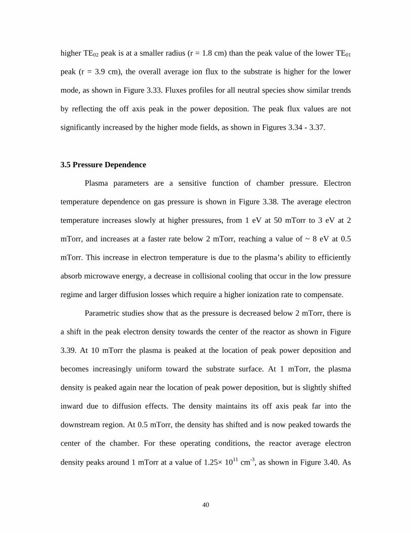
3.5 Pressure Dependence

Plasma parameters are a sensitive function of chamber pressure. Electron

temperature dependence on gas pressure is shown in Figure 3.38. The average electron

temperature increases slowly at higher pressures, from 1 eV at 50 mTorr to 3 eV at 2

mTorr, and increases at a faster rate below 2 mTorr, reaching a value of ~ 8 eV at 0.5

mTorr. This increase in electron temperature is due to the plasma’s ability to efficiently

absorb microwave energy, a decrease in collisional cooling that occur in the low pressure

regime and larger diffusion losses which require a higher ionization rate to compensate.

Parametric studies show that as the pressure is decreased below 2 mTorr, there is

a shift in the peak electron density towards the center of the reactor as shown in Figure

3.39. At 10 mTorr the plasma is peaked at the location of peak power deposition and

becomes increasingly uniform toward the substrate surface. At 1 mTorr, the plasma

density is peaked again near the location of peak power deposition, but is slightly shifted

inward due to diffusion effects. The density maintains its off axis peak far into the

downstream region. At 0.5 mTorr, the density has shifted and is now peaked towards the

center of the chamber. For these operating conditions, the reactor average electron

density peaks around 1 mTorr at a value of 1.25× 1011 cm-3, as shown in Figure 3.40. As

41

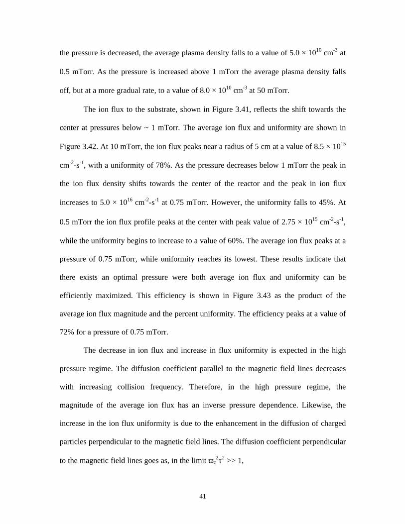
the pressure is decreased, the average plasma density falls to a value of 5.0 × 1010 cm-3 at

0.5 mTorr. As the pressure is increased above 1 mTorr the average plasma density falls

off, but at a more gradual rate, to a value of 8.0 × 1010 cm-3 at 50 mTorr.

The ion flux to the substrate, shown in Figure 3.41, reflects the shift towards the

center at pressures below ~ 1 mTorr. The average ion flux and uniformity are shown in

Figure 3.42. At 10 mTorr, the ion flux peaks near a radius of 5 cm at a value of 8.5 × 1015

cm-2-s-1, with a uniformity of 78%. As the pressure decreases below 1 mTorr the peak in

the ion flux density shifts towards the center of the reactor and the peak in ion flux

increases to 5.0 × 1016 cm-2-s-1 at 0.75 mTorr. However, the uniformity falls to 45%. At

0.5 mTorr the ion flux profile peaks at the center with peak value of 2.75 × 1015 cm-2-s-1,

while the uniformity begins to increase to a value of 60%. The average ion flux peaks at a

pressure of 0.75 mTorr, while uniformity reaches its lowest. These results indicate that

there exists an optimal pressure were both average ion flux and uniformity can be

efficiently maximized. This efficiency is shown in Figure 3.43 as the product of the

average ion flux magnitude and the percent uniformity. The efficiency peaks at a value of

72% for a pressure of 0.75 mTorr.

The decrease in ion flux and increase in flux uniformity is expected in the high

pressure regime. The diffusion coefficient parallel to the magnetic field lines decreases

with increasing collision frequency. Therefore, in the high pressure regime, the

magnitude of the average ion flux has an inverse pressure dependence. Likewise, the

increase in the ion flux uniformity is due to the enhancement in the diffusion of charged

particles perpendicular to the magnetic field lines. The diffusion coefficient perpendicular

to the magnetic field lines goes as, in the limit ωc2τ2 >> 1,

42

2c

m

m

KT D

ω

ν=⊥ . (3.5.1)

In the low pressure regime, the average ion flux magnitude decreases with

decreasing pressure, while the peak-average percent uniformity increases. More

significantly, the peak in the plasma density profile shifts toward the center of the reactor

suggesting enhanced diffusion perpendicular the magnetic field lines. Such a result is

counter-intuitive, since diffusion across the magnetic field lines decreases with

decreasing collision frequency. At lower pressures, the collision frequency is expected to

decrease accordingly. This increase in collision frequency at lower pressures can be

attributed to an increase in the electron temperature. The momentum transfer rate

coefficient increases with increasing electron temperature, as shown in Figure 3.44. The

momentum transfer rate coefficient and the neutral gas density versus chamber pressure

is shown in Figure 3.45. At low pressures, rate coefficient is exponentially increasing due

to the rise in the electron temperature. As the pressure increases, the temperature

decreases thereby decreasing the value of the rate coefficient. Likewise, as the pressure

increases so does the neutral gas density. The collision frequency, which is the product of

the momentum transfer rate coefficient and the neutral gas density, is sensitive to

temperature in the low pressure regime, while it becomes dependent to neutral gas

densities in the high pressure regime. This increase of the collision frequency in the low

pressure regime produces enhancement diffusion of charged particles across the magnetic

field lines. Overall, diffusion losses are enhanced in both the low and high pressure

regimes. There exists an optimal pressure for charged particle confinement, maximizing

ion flux to the substrate surface, and flux profile uniformity.

43

3.6 References

1. S. Rauf and M. J. Kushner, J. Appl. Phys., vol. 81, p. 5966, 1997.

2. R.Hidaka, T. Yamaguchi, N. Hirotsu, T. Ohshima, R. Koga, M. Tanaka, and Y.

Kawai, Jpn. J. Appl. Phys., vol. 32, p. 174, 1993.

3. C. A. Outten, J. C. Barbour, and W. R. Wampler, J. Vac. Sci. Technol. A, vol. 9, p.

717, 1991.

4. J. E. Stevens, J. L. Cecchi, Y. C. Huang, and R. L. Jarecki, Jr., J. Vac. Sci. Technol.

A, vol. 9, p. 696, 1991.

5. M. D. Bowden, T. Okamoto, F. Kimura, H.Muta, K. Uchino, and K. Muraoka, J.

Appl. Phys., vol. 73, p. 2732, 1993.

6. D. C. Cartwright, S. Trajmar, A. Chutjian, and W. Williams, Physc. Rev. A, vol. 16, p.

1041, 1977

7. R. T. Brinkman and S. Trajmar, Ann. Geophysc. vol. 26, p. 201, 1970

8. W. L. Borst, Physc.Rev. A, vol. 5, p. 648, 1972

9. S. Geltman, J. Quant. Spect. Rad. Transfer, vol. 13, p. 601, 1973

44

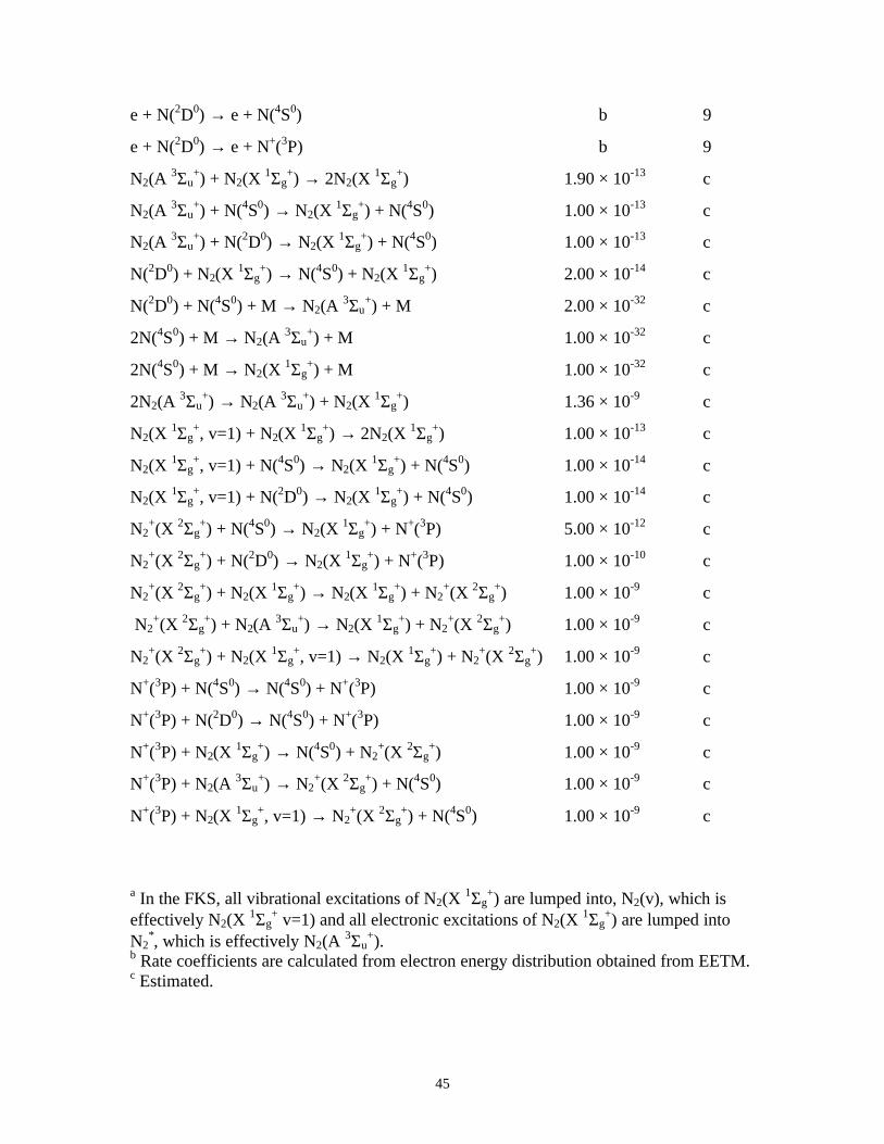
Table 3.1 Gas phase reactions for N2.

Reaction Rate Coefficient Ref.

e + N2(Χ 1Σg+) → e + N2(Χ 1Σg

+, v=1) b 6

e + N2(Χ 1Σg+) → e + N2(Χ 1Σg

+, v=2) b 6

e + N2(Χ 1Σg+) → e + N2(Χ 1Σg

+, v=3) b 6

e + N2(Χ 1Σg+) → e + N2(Χ 1Σg

+, v=4) b 6

e + N2(Χ 1Σg+) → e + N2(Χ 1Σg

+, v=5) b 6

e + N2(Χ 1Σg+) → e + N2(Χ 1Σg

+, v=6 b 6

e + N2(Χ 1Σg+) → e + N2(Χ 1Σg

+, v=7) b 6

e + N2(Χ 1Σg+) → e + N2(Χ 1Σg

+, v=8) b 6

e + N2(Χ 1Σg+) → e + N2(A 3Σu

+) b 7

e + N2(Χ 1Σg+) → e + N2(B 3Πg) b 7

e + N2(Χ 1Σg+) → e + N2(B

1 3Σu-) b 8

e + N2(Χ 1Σg+) → e + N2(a

1 3Σu-) b 8

e + N2(Χ 1Σg+) → e + N2(C 3Πu) b 8

e + N2(Χ 1Σg+) → e + N(4S0) + N(2D0) b 6

e + N2(Χ 1Σg+) → 2e + N2

+(Χ 2Σg+) b 6

e + N2(Χ 1Σg+, v=1) → e + N2(Χ 1Σg

+) b 6

e + N2(Χ 1Σg+, v=1) → e + N2(A 3Σu

+) b 6

e + N2(Χ 1Σg+, v=1) → 2e + N2

+(Χ 2Σg+) b 6

e + N2(A 3Σu+) → e + N2(Χ 1Σg

+, v=1) b 6

e + N2(A 3Σu+) → e + N2(Χ 1Σg

+) b 6

e + N2(A 3Σu+) → 2e + N2

+(Χ 2Σg+) b 6

e + N2+(Χ 2Σg

+) → N(2D0) + N(4S0) 1.00 × 10-7 c

e + N(4S0) → e + N(2D0) b 9

e + N(4S0) → e + N(2P0) b 9

e + N(4S0) → 2e + N+(3P) b 9

45

e + N(2D0) → e + N(4S0) b 9

e + N(2D0) → e + N+(3P) b 9

N2(A 3Σu+) + N2(Χ 1Σg

+) → 2N2(Χ 1Σg+) 1.90 × 10-13 c

N2(A 3Σu+) + N(4S0) → N2(Χ 1Σg

+) + N(4S0) 1.00 × 10-13 c

N2(A 3Σu+) + N(2D0) → N2(Χ 1Σg

+) + N(4S0) 1.00 × 10-13 c

N(2D0) + N2(Χ 1Σg+) → N(4S0) + N2(Χ 1Σg

+) 2.00 × 10-14 c

N(2D0) + N(4S0) + M → N2(A 3Σu+) + M 2.00 × 10-32 c

2N(4S0) + M → N2(A 3Σu+) + M 1.00 × 10-32 c

2N(4S0) + M → N2(Χ 1Σg+) + M 1.00 × 10-32 c

2N2(A 3Σu+) → N2(A 3Σu

+) + N2(Χ 1Σg+) 1.36 × 10-9 c

N2(Χ 1Σg+, v=1) + N2(Χ 1Σg

+) → 2N2(Χ 1Σg+) 1.00 × 10-13 c

N2(Χ 1Σg+, v=1) + N(4S0) → N2(Χ 1Σg

+) + N(4S0) 1.00 × 10-14 c

N2(Χ 1Σg+, v=1) + N(2D0) → N2(Χ 1Σg

+) + N(4S0) 1.00 × 10-14 c

N2+(Χ 2Σg

+) + N(4S0) → N2(Χ 1Σg+) + N+(3P) 5.00 × 10-12 c

N2+(Χ 2Σg

+) + N(2D0) → N2(Χ 1Σg+) + N+(3P) 1.00 × 10-10 c

N2+(Χ 2Σg

+) + N2(Χ 1Σg+) → N2(Χ 1Σg

+) + N2+(Χ 2Σg

+) 1.00 × 10-9 c

N2+(Χ 2Σg

+) + N2(A 3Σu+) → N2(Χ 1Σg

+) + N2+(Χ 2Σg

+) 1.00 × 10-9 c

N2+(Χ 2Σg

+) + N2(Χ 1Σg+, v=1) → N2(Χ 1Σg

+) + N2+(Χ 2Σg

+) 1.00 × 10-9 c

N+(3P) + N(4S0) → N(4S0) + N+(3P) 1.00 × 10-9 c

N+(3P) + N(2D0) → N(4S0) + N+(3P) 1.00 × 10-9 c

N+(3P) + N2(Χ 1Σg+) → N(4S0) + N2

+(Χ 2Σg+) 1.00 × 10-9 c

N+(3P) + N2(A 3Σu+) → N2

+(Χ 2Σg+) + N(4S0) 1.00 × 10-9 c

N+(3P) + N2(Χ 1Σg+, v=1) → N2

+(Χ 2Σg+) + N(4S0) 1.00 × 10-9 c

a In the FKS, all vibrational excitations of N2(Χ 1Σg+) are lumped into, N2(v), which is

effectively N2(Χ 1Σg+ v=1) and all electronic excitations of N2(Χ 1Σg

+) are lumped intoN2

*, which is effectively N2(A 3Σu+).

b Rate coefficients are calculated from electron energy distribution obtained from EETM.c Estimated.

Magnetic Coils

WaferPumpPort

Gas Ring

DielectricWindow

Figure 3.1 Typical electron cyclotron resonance (ECR) tool used for materials processing.

46

Figure 3.2 Magnetic field configuration inside the ECR reactor. Vector arrows (black) represent magnetic flux lines and contour lines (red) represent magnetic field intensities.

47

0

30

Radius (cm)20020

626 626

756 756

519519

847 847

911911

Figure 3.3 Azimuthal electric field component and axial magnetic field component of the incident electromagnetic field (b) plasma conductivity and power deposition inside the ECR processing tool for base case conditions.

48

0 2020

0

30

Radius (cm)

(Gauss)

5.0 x 101

5.0 x 10-2

(V / cm)

Azimuthal Electric Field Axial Magnetic Field

(W / cm3)

0 2020

0

30

Radius (cm)

(1 / Ω1 cm2)

Conductivity Power Deposition

(a)

(b)

1.5 x 101

1.0 x 10-35.0 x 10-6

5.0 x 10-2

2.0 x 102

0.0

Figure 3.4 Axial profiles of (a) plasma conductivity and static magnetic field (b) azimuthal electric field intensity and power deposition for base case conditions at a radius of 5 cm.

49

0

40

80

120

160

200 102

101

100

10-1

10-2

10-3

10-40 10 20

Reactor Height (cm)

Power E-Field

10-1

10-2

10-3

10-4

10-5

10-6 0

200

400

600

800

1000

10 200Reactor Height (cm)

Wafer

Resonance Zone

ConductivityB-Field

(a)

(b)

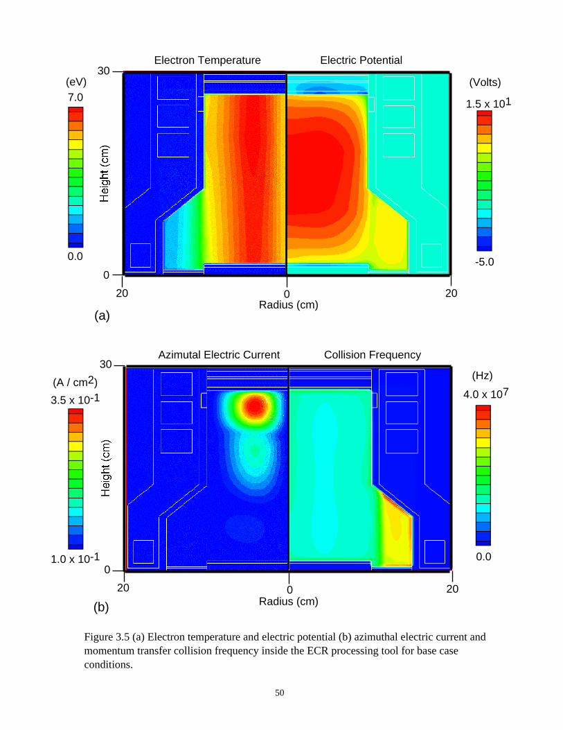
Figure 3.5 (a) Electron temperature and electric potential (b) azimuthal electric current and momentum transfer collision frequency inside the ECR processing tool for base case conditions.

50

0 2020

0

30

1.5 x 101

(eV)7.0

0.0

Electron Temperature Electric Potential

(Volts)

Radius (cm)(a)

20

0

30

(A / cm2)

0 20Radius (cm)

Azimutal Electric Current Collision Frequency

(Hz)

(b)

-5.0

3.5 x 10-1

1.0 x 10-1

4.0 x 107

0.0

Figure 3.6 (a) Electron density and electron source (ionization rate) (b) N2 gas density and

N2 source inside the ECR processing tool for base case conditions. Black vector lines in

(b) represent gas flow.

51

0.0

20

0

30

3.0 x 1011

1.0 x 1010

0 20Radius (cm)

Electron Electron Source

(cm-3 s-1) (cm-3)

0.0

20

0

30

1.5 x 1013

1.0 x 1012

0 20Radius (cm)

N2 N2 Source

(cm-3 s-1) (cm-3)

-6.0 x 1016

(a)

(b)

3.0 x 1016

Figure 3.7 (a) N2(v) density and N2(v) source (b) N2* density and N2* source inside the

ECR processing tool for base case conditions.

52

3.0 x 1015

-3.0 x 1015

20

0

30

(cm-3)

3.5 x 1012

0 20Radius (cm)

N2(V) N2(V) Source

(cm-3 s-1)

(a)

4.0 x 1016

0.0

20

0

30

3.5 x 1012

1.0 x 1011

0 20Radius (cm)

N2* N2* Source

(cm-3 s-1) (cm-3)

(b)

1.0 x 1011

Figure 3.8 (a) N density and N source (b) N* gas density and N* source inside the ECR processing tool for base case conditions.

53

-1.0 x 1015

20

0

30

8.0 x 1012

4.0 x 1012

0 20Radius (cm)

N N Source

(cm-3 s-1) (cm-3)

0.0

20

0

30

3.0 x 1012

1.0 x 1011

0 20Radius (cm)

N* N* Source

(cm-3 s-1) (cm-3)

4.0 x 1015

9.0 x 1015

(a)

(b)

Figure 3.9 (a) N2+ density and N2+ source rate (b) N+ density and N+ source inside the

ECR processing tool for base case conditions.

54

7.0 x 1015

0.0

20

0

30

7.0 x 1010

1.0 x 109

0 20Radius (cm)

N+ N+ Source

(cm-3 s-1) (cm-3)

1.0 x 1016

-1.0 x 1014

20

0

30

2.0 x 1011

1.0 x 1010

0 20Radius (cm)

N2+ N2+ Source

(cm-3 s-1) (cm-3)

(a)

(b)

Figure 3.10 Experimetal and computed radial profiles of the ion saturation current density in an ECR processign tool for a TE01 electric field mode.

55

Radius (cm)0 5 10510

0

10

20

30

40

Experimental(R. Hidaka et al.)

Theoretical

N2, 0.5 mTorr, 3 kW

Figure 3.11 Experimetal and computed values of the ion saturation current density for a TE01 electric field mode with varying power.

56

Microwave Power (kW)

1 20

10

20

Experimental(R. Hidaka et al.)

Theoretical

N2, 0.5 mTorr

0

Figure 3.12 Magnetic flux in the ECR processing tool (a) without activation of the magnetic subcoil (b) with activation of the magnetic subcoil.

57

0Radius (cm)

(a)

020

30

20 0Radius (cm)

(b)

30

0

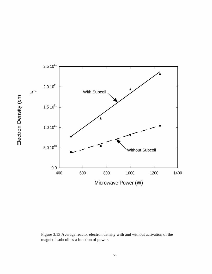
Figure 3.13 Average reactor electron density with and without activation of the magnetic subcoil as a function of power.

58

0.0

5.0 1010

1.0 1011

1.5 1011

2.0 1011

2.5 1011

400 600 800 1000 1200 1400

Ele

ctro

n D

en

sity

(cm

-3)

Microwave Power (W)

With Subcoil

Without Subcoil

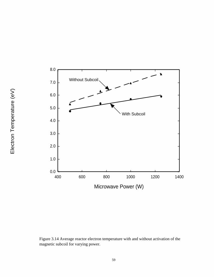
0.0

1.0

2.0

3.0

4.0

5.0

6.0

7.0

8.0

400 600 800 1000 1200 1400

Ele

ctro

n T

em

pe

ratu

re (

eV

)

Microwave Power (W)

Figure 3.14 Average reactor electron temperature with and without activation of the magnetic subcoil for varying power.

59

With Subcoil

Without Subcoil

Figure 3.15 Ion to neutral density with and without activation of the magnetic subcoil as a function of power.

60

0.0 100

5.0 10-3

1.0 10-2

1.5 10-2

400 600 800 1000 1200 1400

Ion/N

eutr

al D

ensi

ty

Microwave Power (W)

With Subcoil

Without Subcoil

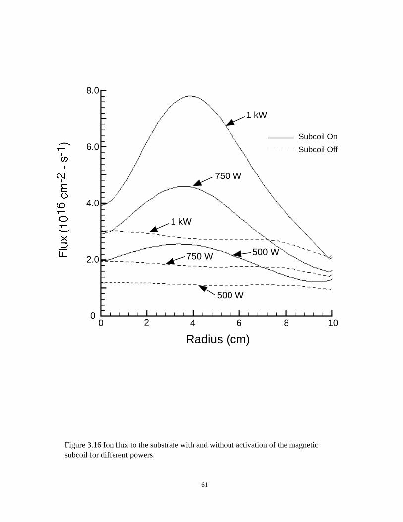
Figure 3.16 Ion flux to the substrate with and without activation of the magnetic subcoil for different powers.

61

Radius (cm)0 2 4 6 8 10

0

2.0

4.0

6.0

8.0

1 kW

1 kW

750 W

750 W 500 W

500 W

Subcoil On

Subcoil Off

Figure 3.17 N2(v) flux to the substrate with and without activation of the magnetic

subcoil for different powers.

62

Radius (cm)0 2 4 6 8 10

0

2.0

4.0

6.01 kW

1 kW

750 W

750 W500 W

500 W

Subcoil On

Subcoil Off

Radius (cm)0 2 4 6 8 10

0

2.0

4.0

6.0

1 kW

1 kW

750 W

750 W

500 W

500 W

Subcoil On

Subcoil Off

Figure 3.18 N2* flux to the substrate with and without activation of the magnetic

subcoil for different powers.

63

Radius (cm)0 2 4 6 8 10

0

2.0

1.5

2.5

1 kW

1 kW

750 W

750 W

500 W

500 W

Subcoil On

Subcoil Off

1.0

0.5

Figure 3.19 Atomic nitrogen, N, flux to the substrate with and without activation of the magnetic subcoil for different powers.

64

Radius (cm)0 2 4 6 8 10

0

4.0

3.0

5.0

1 kW

1 kW

750 W

750 W

500 W

500 W

Subcoil On

Subcoil Off

2.0

1.0

6.0

Figure 3.20 N* flux to the substrate with and without activation of the magnetic subcoil for different powers.

65

Figure 3.21 Ion flux to the substrate with and without activation of the magnetic subcoil for different pressures.

66

Radius (cm)

0 2 4 6 8 100

1

2

3

4

5

10 mTorr

10 mTorr

1 mTorr

1 mTorr

Subcoil On

Subcoil Off

Radius (cm)

0 2 4 6 8 100

1

2

3

4

510 mTorr

10 mTorr

1 mTorr1 mTorr

Subcoil On

Subcoil Off

6

7

Figure 3.22 N2(v) flux to the substrate with and without activation of the magnetic

subcoil for different pressures.

67

Radius (cm)

0 2 4 6 8 100

2

4

6

8

10

10 mTorr

10 mTorr

1 mTorr

1 mTorr

Subcoil On

Subcoil Off

Figure 3.23 N* flux to the substrate with and without activation of the magnetic subcoil for different pressures.

68

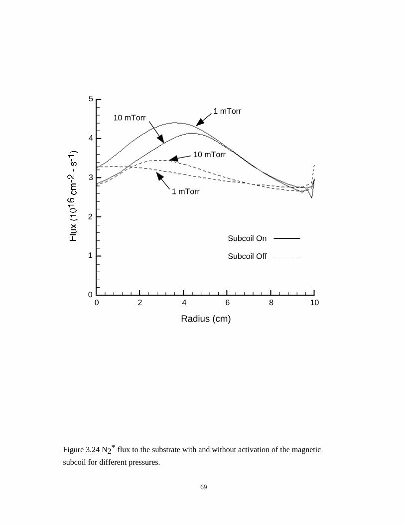
Radius (cm)

0 2 4 6 8 100

1

2

3

4

5

10 mTorr

10 mTorr1 mTorr

1 mTorr

Subcoil On

Subcoil Off

Figure 3.24 N2* flux to the substrate with and without activation of the magnetic

subcoil for different pressures.

69

Radius (cm)

0 2 4 6 8 100

1

2

3

4

5 10 mTorr

10 mTorr

1 mTorr

1 mTorr

Subcoil On

Subcoil Off

Figure 3.25 Flux of atomic nitrogen, N, to the substrate with and without activation of the magnetic subcoil for different pressures.

70

Figure 3.26 Azimuthal electric field component and axial magnetic field component of incident electromagnetic field (b) power deposition and electron temperature inside the ECR processing tool.

71

2.5 x 10-2

20

0

30

200

0

20Radius (cm)

Azimuthal Electric Field Axial Magnetic Field

(Gauss) (V / cm)

2.5 x 101

0(a)

0

20

0

30

2.0 x 101

2.0 x 10-2

20

Radius (cm)

Power Deposition Electron Temperature

(eV) (W / cm3)

7.5

0

(b)

Figure 3.27 Radial profiles of electron temperature and power deposition for the (a) TE01 (b) TE02 mode in the resonance zone (z=20 cm).

72

Power

Temperature

Temperature

Power

Radius (cm)

Radius (cm)80 2 4 6 10

80 2 4 6 10

TE01

TE02

0

2

4

6

10

8

0

4

8

12

20

16

0

2

4

6

10

8

0

4

8

12

20

16

a)

b)

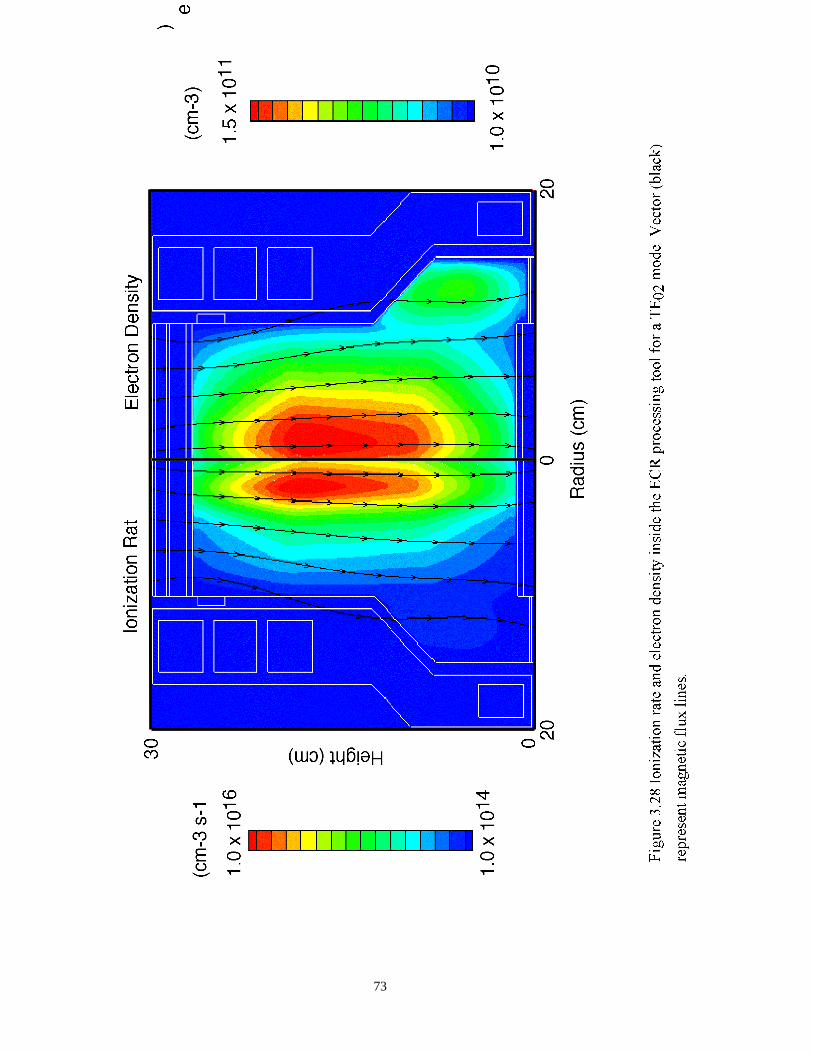
73

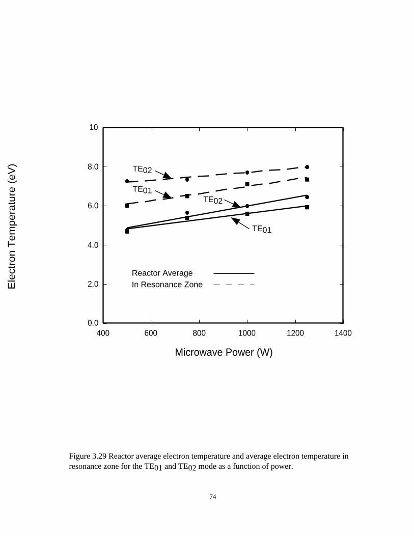
0.0

2.0

4.0

6.0

8.0

10

400 600 800 1000 1200 1400

Ele

ctro

n T

em

pe

ratu

re (

eV

)

Microwave Power (W)

Figure 3.29 Reactor average electron temperature and average electron temperature in resonance zone for the TE01 and TE02 mode as a function of power.

74

Reactor AverageIn Resonance Zone

TE01

TE02

TE01TE02

0.0

1.0 1011

2.0 1011

3.0 1011

4.0 1011

5.0 1011

6.0 1011

7.0 1011

8.0 1011

400 600 800 1000 1200 1400

Ele

ctro

n D

en

sity

(cm

-3)

Microwave Power (W)

Figure 3.30 Reactor average electron density and average electron density in resonance zone for the TE01 and TE02 mode as a function of power.

75

Reactor AverageIn Resonance Zone

TE01

TE02

TE01

TE02

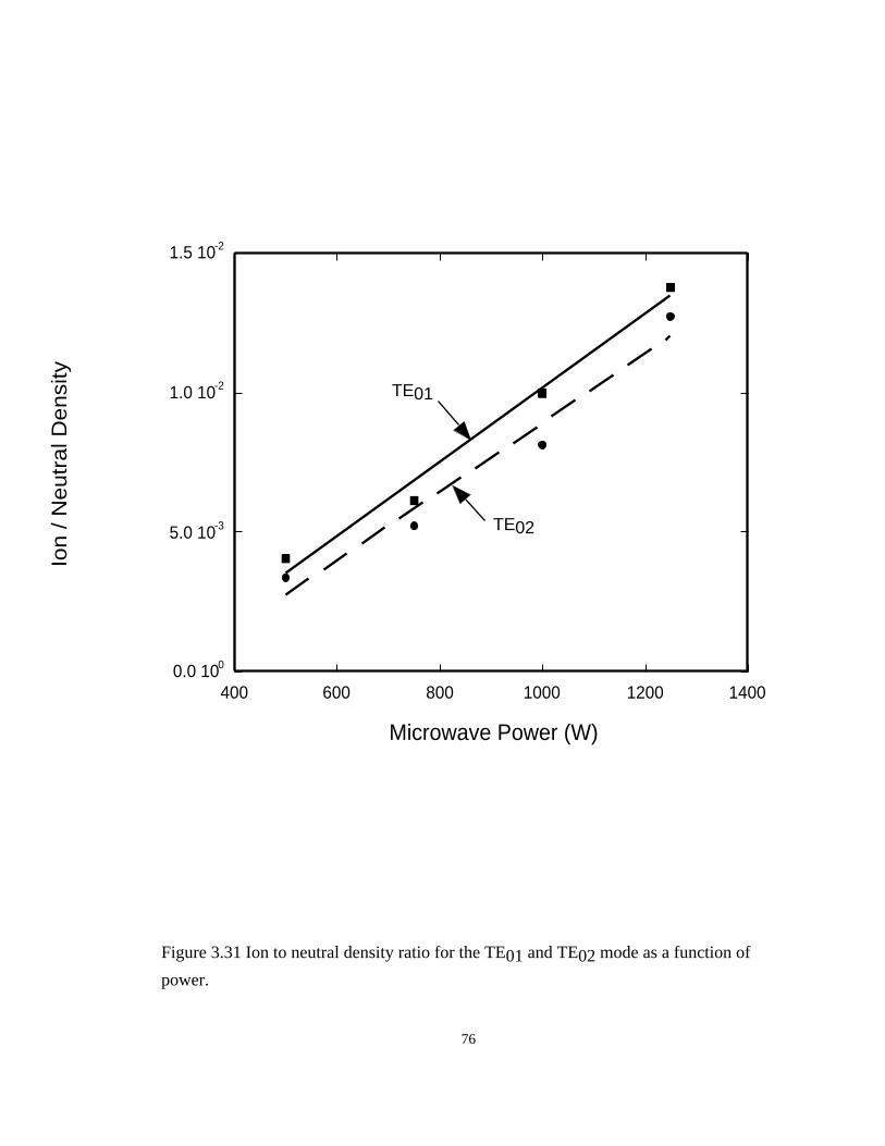
0.0 100

5.0 10-3

1.0 10-2

1.5 10-2

400 600 800 1000 1200 1400

Ion

/ N

eu

tra

l De

nsi

ty

Microwave Power (W)

Figure 3.31 Ion to neutral density ratio for the TE01 and TE02 mode as a function of

power.

76

TE02

TE01

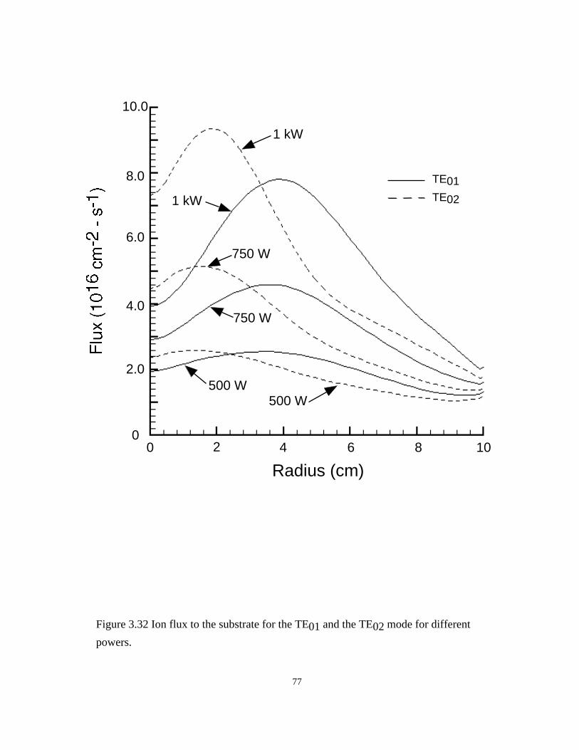
Radius (cm)0 2 4 6 8 10

0

2.0

4.0

6.0

1 kW

1 kW

750 W

750 W

500 W500 W

TE01TE02

8.0

10.0

Figure 3.32 Ion flux to the substrate for the TE01 and the TE02 mode for different

powers.

77

0.0 100

1.0 1016

2.0 1016

3.0 1016

4.0 1016

5.0 1016

6.0 1016

400 500 600 700 800 900 1000 1100

Flu

x (c

m-2

s-1

)

Microwave Power (W)

Figure 3.33 Average ion flux to the substrate for the TE01 and TE02 mode as a

function of power.

78

TE02

TE01

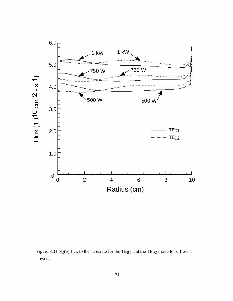
Radius (cm)0 2 4 6 8 10

0

2.0

4.0

6.0

1 kW 1 kW

750 W 750 W

500 W500 W

TE01TE02

1.0

3.0

5.0

Figure 3.34 N2(v) flux to the substrate for the TE01 and the TE02 mode for different

powers.

79

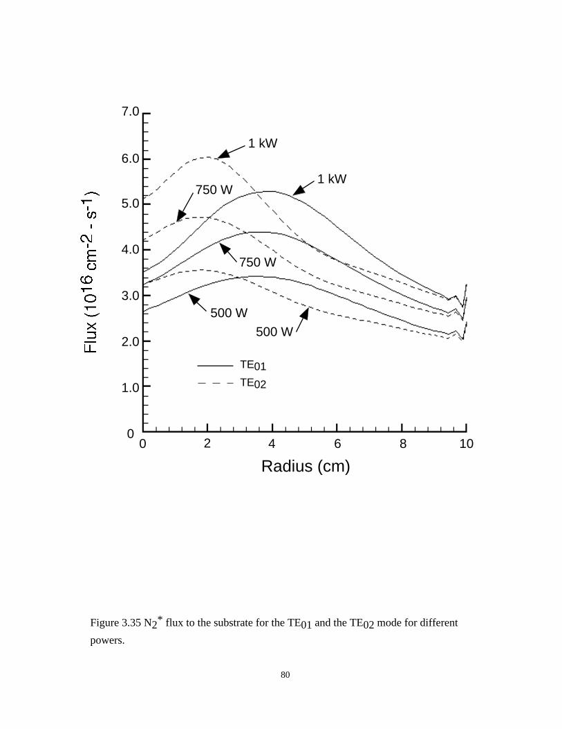
Radius (cm)0 2 4 6 8 10

0

2.0

4.0

7.0

1 kW

1 kW750 W

750 W

500 W

500 W

TE01TE021.0

3.0

5.0

6.0

Figure 3.35 N2* flux to the substrate for the TE01 and the TE02 mode for different

powers.

80

Radius (cm)0 2 4 6 8 10

0

1.0

2.5 1 kW

1 kW

750 W 750 W

500 W

500 W

TE01TE02

0.5

2.0

1.5

Figure 3.36 Flux of atomic nitrogen, N, to the substrate for the TE01 and the TE02

mode for different powers.

81

Radius (cm)0 2 4 6 8 10

0

2.0

6.0

1 kW1 kW

750 W 750 W

500 W

500 W

TE01TE021.0

4.0

3.0

5.0

Figure 3.37 N* flux to the substrate for the TE01 and the TE02 mode for different

powers.

82

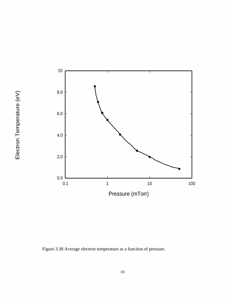
Figure 3.38 Average electron temperature as a funciton of pressure.

83

0.0

2.0

4.0

6.0

8.0

10

0.1 1 10 100

Ele

ctro

n T

em

pe

ratu

re (

eV

)

Pressure (mTorr)

84

Figure 3.40 Reactor average electron density as a function of pressure.

85

0.0

5.0 1010

1.0 1011

1.5 1011

2.0 1011

0.1 1 10 100

Ele

ctro

n D

en

sity

(cm

-3)

Pressure (mTorr)

Figure 3.41 Ion flux as a function of radius for varying chamber pressure.

86

Radius (cm)

10

1

0.5

100

• N2, 750 Watts, 10 sccm, TE(0,1) mode

5.0 x 1016

0.0

(cm-2 s-1)

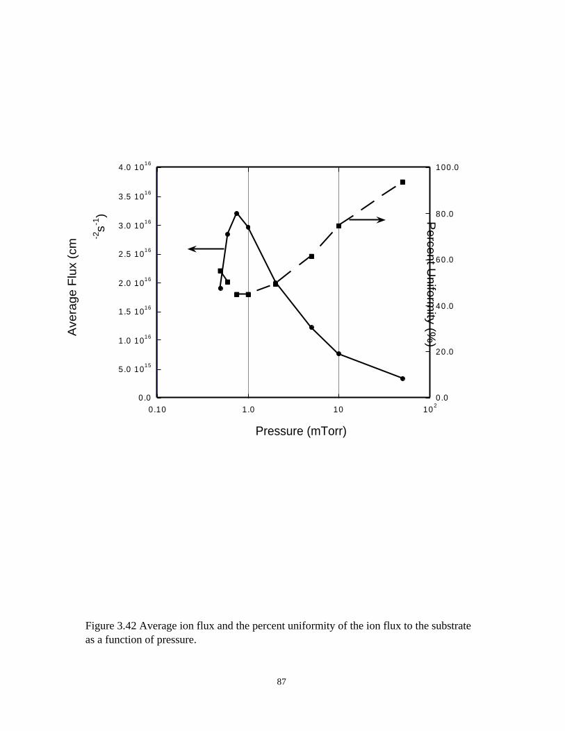
0.0

5.0 1015

1.0 1016

1.5 1016

2.0 1016

2.5 1016

3.0 1016

3.5 1016

4.0 1016

0.0

20.0

40.0

60.0

80.0

100.0

0.10 1.0 10 102

Ave

rag

e F

lux

(cm

-2s-1

) Perce

nt U

nifo

rmity (%

)

Pressure (mTorr)

Figure 3.42 Average ion flux and the percent uniformity of the ion flux to the substrate as a function of pressure.

87

Figure 3.43 Efficiency as a function of pressure. The “efficiency” is defined as the product of the average flux and the percent uniformity.

88

0.0

0.20

0.40

0.60

0.80

1.0

0.10 1.0 10 102

Effi

cien

cy

Pressure (mTorr)

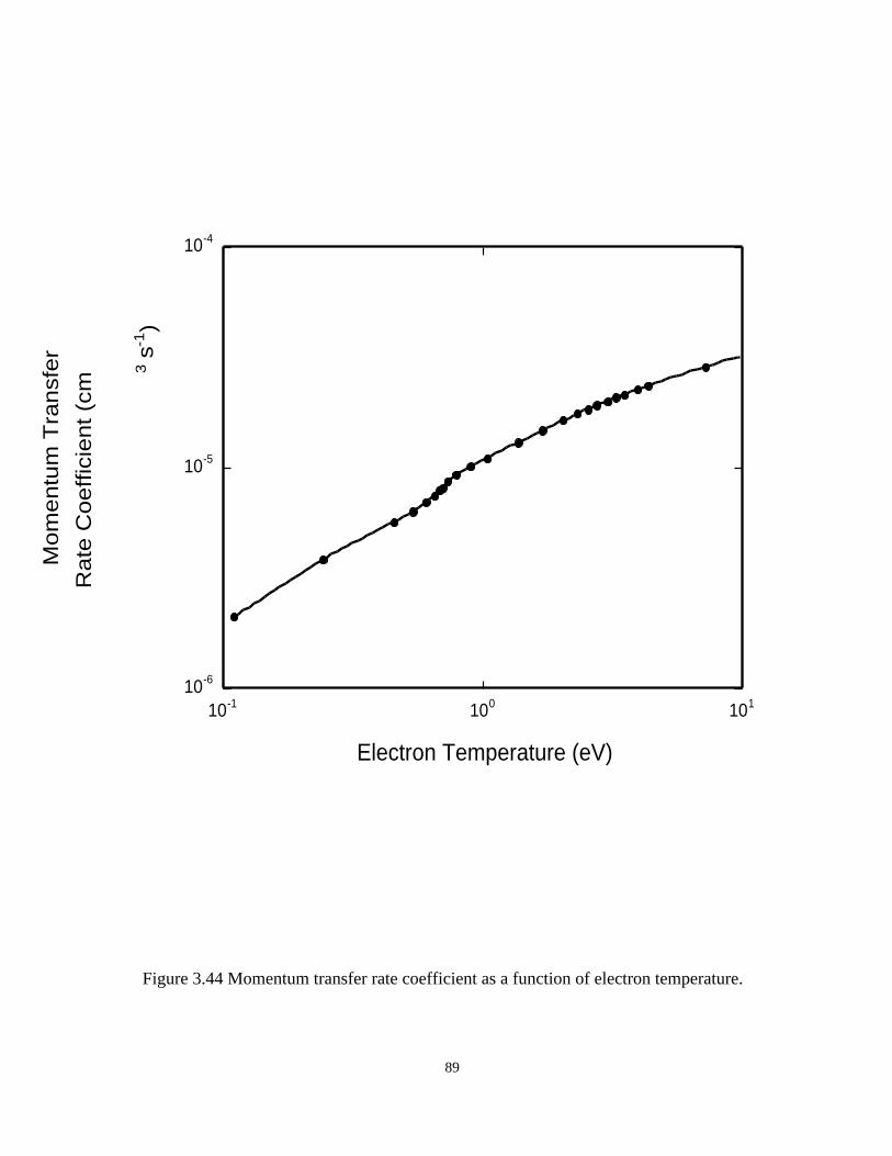
10-6

10-5

10-4

10-1 100 101

Mo

me

ntu

m T

ran

sfe

r

Ra

te C

oe

ffic

ien

t (c

m

3 s

-1)

Electron Temperature (eV)

Figure 3.44 Momentum transfer rate coefficient as a function of electron temperature.

89

Figure 3.45 Average mometum transfer rate coefficient and neutral gas density as a function of pressure.

90

0

1 10-5

2 10-5

3 10-5

4 10-5

0

2 1014

4 1014

6 1014

8 1014

1 1015

10-1 100 101 102

Neutra

l Gas D

ensity (cm

-3)

Pressure (mTorr)

Mom

entu

m T

ransf

er

Rate

Coeffic

ient (c

m

3 s

-1)

TemperatureDependence

Regime

PressureDependence

Regime

91

IV. Conclusions

A finite-difference-time-domain (FDTD) simulation for microwave injection and

propagation has been developed to examine the spatial coupling of microwave radiation

to the plasma in an electron cyclotron resonance (ECR) reactor. Microwave coupling is a

concern due to issues related to the uniformity of dissociation, electron heating, and

ultimately process uniformity. The FDTD simulation was incorporated as a module in the

2-dimensional Hybrid Plasma Equipment Model (HPEM). Plasma dynamics were

coupled to the electromagnetic fields through a tensor form of Ohm’s law. Power

deposition calculated in the FDTD module is then used in solving the electron energy

equation. Consequences of mode structure, magnetic field configuration, and operating

conditions on plasma parameters and fluxes to the substrate in ECR sources for materials

processing were examined with this model.

The computed radial distribution of the ion saturation current density showed

good agreement with experiment. The radial ion saturation current density in the case of

the TE01 mode was uniform within 5% over an 8 inch diameter. Parametric studies in

which microwave power was varied showed that theoretical predictions followed

experimental trends, with the saturation current increasing linearly in proportion to

microwave power.

Results with varying magnetic coil configurations showed that when operating

with the subcoil the ion flux to the substrate reflected the reactor ion density profiles. An

increase in power level leads to the enhancement of any non-uniformities present in the

92

flux profile. At higher pressures the sensitivity of the ion flux to activation of the subcoil

is decreased and the uniformity of the ion flux is increased.

It was shown that the higher order circular TEon modes have several off axis peaks

in the electric field depending on the harmonic mode, n, used. The power deposition

exhibits a semi-Lorentzian line shape in the axial direction and reflects the incident

electric field profile in the radial direction. However, production of several off axis peaks

in the power deposition does not necessarily enhance the uniformity of the flux incident

onto the substrate. The distance of the resonance zone to the substrate and the magnetic

field configuration determined the extent that higher order modes enhanced uniformity of

the flux to the substrate. Overall, diffusion losses are enhanced in both the low and high

pressure regimes. Results suggest that there is an optimal pressure for charged particle

confinement, maximizing ion flux to the substrate surface, and flux profile uniformity.