CONNECTIVITY ASSESSMENT OF CHANGES IN WETLAND ECOSYSTEMS FROM 1946 TO 2003 IN THE

RESORT MUNICIPALITY OF WHISTLER, BRITISH COLUMBIA.

Lindsay McBlane Bachelor of Arts (Geography), Simon Fraser University, 2004

RESEARCH PROJECT SUBMITTED IN PARTIAL FULFILLMENT OF THE REQUIREMENTS FOR THE DEGREE OF

MASTER O F RESOURCE MANAGEMENT

In the School of Resource and Environmental Management

of the Faculty of Applied Sciences

Report no. 423

0 Lindsay McBlane 2007

SIMON FRASER UNIVERSITY

Spring 2007

All rights reserved. This work may not be reproduced in whole or in part, by photocopy

or other means, without permission of the author.

APPROVAL

Name: Lindsay McBlane

Degree: Master of Resource Management

Title of Research Project: Connectivity Assessment of Changes in Wetland Ecosystems from 1946 to 2003 in the Resort Municipality of Whistler, British Columbia

Project No. 423

Supervisory Committee:

Chair: Ms. Shelley Marshall Department of Resource and Environmental Management

Date DefendedtApproved:

Dr. Kristina Rothley Senior Supervisor Associate Professor / Department of Resource and Environmental Management

Dr. Suzana Dragicevic Supervisor Associate Professor / Department of Geography

Dr. Arthur Roberts Supervisor Professor / Department of Geography

R'Zl SIMON FRASER p y 4.c U N ~ E R S ~ T V ~ ~ ~ ~ ~ Y

DECLARATION OF PARTIAL COPYRIGHT LICENCE

The author, whose copyright is declared on the title page of this work, has granted to Simon Fraser University the right to lend this thesis, project or extended essay to users of the Simon Fraser University Library, and to make partial or single copies only for such users or in response to a request from the library of any other university, or other educational institution, on its own behalf or for one of its users.

The author has further granted permission to Simon Fraser University to keep or make a digital copy for use in its circulating collection (currently available to the public at the "Institutional Repository" link of the SFU Library website ~www.lib.sfu.ca> at: ~http:llir.lib.sfu.calhandlell8921112>) and, without changing the content, to translate the thesislproject or extended essays, if technically possible, to any medium or format for the purpose of preservation of the digital work.

The author has further agreed that permission for multiple copying of this work for scholarly purposes may be granted by either the author or the Dean of Graduate Studies.

It is understood that copying or publication of this work for financial gain shall not be allowed without the author's written permission.

Permission for public performance, or limited permission for private scholarly use, of any multimedia materials forming part of this work, may have been granted by the author. This information may be found on the separately catalogued multimedia material and in the signed Partial Copyright Licence.

The original Partial Copyright Licence attesting to these terms, and signed by this author, may be found in the original bound copy of this work, retained in the Simon Fraser University Archive.

Simon Fraser University Library Burnaby, BC, Canada

Revised: Spring 2007

ABSTRACT

Wetlands throughout the Resort Municipality of Whistler (RMOW) are becoming

smaller and more fragmented due to development and introduction of linear features:

roads and railways. Landscape changes may result in negative consequences for wetland

ecosystems, including reducing genetic diversity and decreasing species populations.

Using aerial photographs, 1946-2003, this study focused on spatial and temporal changes

in extent, patch size, and connectivity to wetland ecosystems. Connectivity was assessed

with commonly used geometric measures (area, shape index, total edges) together with a

functional, graph-based metric (correlation length). Both geometric and functional

measures of connectivity gave similar results; however. functional measures provided

insight into the effect of changes to the matrix between the wetlands not shown with

solely geometric measures. Overall. total area of wetlands and connectivity throughout

the RMOW decreased significantly. Although wetland habitat patches and landscape

matrix contributed to decreased connectivity. changes to wetland patches themselves had

a stronger effect.

DEDICATION

To my family for everything. You supported me throughout this process, helped

me out when I needed someone to test ideas and my own understanding on, and made me

laugh right when I needed it. The long nights, the motivating thoughts, and the unyielding

pride I saw in your eyes kept me going even while living in a hotel trying to prepare for

my defense and submit my final paper. Thank you for all your guidance, support, and

love over the years.

To my friends, I want to thank you for knowing when to push me to go out and

have a social life as well as when to leave me alone and let me work till the wee hours of

the morning. You all know who you are and I appreciate you for your assistance on this

project, your understanding through some of the rougher times, and your love of the great

outdoors - we can never beat camping and Whistler. Thank you.

ACKNOWLEDGEMENTS

Thank you to Dr. Kristina Rothley who took a chance on me. Your patience in

guiding me through my questions, concerns, and frustrations was greatly appreciated.

Without your support and guidance, this project would not have achieved the results it

has. You are unparalleled as a mentor and always had me considering aspects of this

project that I had never imagined.

Thank you Dr. Suzana Dragicevic and Dr. Arthur Roberts for their open-

mindedness and theu willingness to become involved in this project, which took their

strengths and applied them to a resource management issue.

Thank you to Dan Griffin, Heather Beresford, and Veronica Woodruff for coming

up with the ideas behind the project and providing me with valuable datasets. Without

you, this project would never have gotten started.

TABLE OF CONTENTS

.. Approval ........................................................................................................................ ii ... Abstract ........................................................................................................................ iii

Dedication .................................................................................................................. iv

Acknowledgements .................................................................................................... v

Table of Contents ......................................................................................................... vi ... List of Figures ............................................................................................................. viii

List of Tables ................................................................................................................ x

Glossary ........................................................................................................................ xi

1 Introduction ............................................................................................................ 1 1.1 Overview ........................................................................................................... 1 1.2 Research Questions ......................................................................................... 3

2 Background ............................................................................................................ 4 ..................................................................................... 2.1 Landscape Connectivity 4

2.2 Wetland Ecosystems .......................................................................................... 8 2.3 Study Area ..................................................................................................... 10

3 Methods ................................................................................................................ 14 3.1 Data Collection ................................................................................................ 14

3.1.1 Existing Data ............................................................................................ 14 3.1.2 Aerial Photograph Selection ..................................................................... 15

3.2 Data Creation .................................................................................................. 17 3.2.1 Aerial Photograph Interpretation ............................................................. 17 3.2.2 Digitizing the Data .................................................................................... 20

3.3 SELES Connectivity Analysis ......................................................................... 21 3.3.1 Analysis Extent ......................................................................................... 23 3.3.2 Wetland (Habitat Patch) Surface ............................................................... 23 3.3.3 Calculating Resistance Surfaces ........................................................... 24 3.3.4 Running SELES ....................................................................................... 30

.................................................................................. 3.3.5 Sensitivity Analysis 34 .......................................................... 3.4 Common Connectivity Metrics Analysis 35

................................................................................................................... 4 Results 37 ............................................ 4.1 Correlation Length: Straightforward Comparison 37

................................................. 4.2 Correlation Length: Multifaceted Comparison 43 4.3 Sensitivity Analysis ......................................................................................... 46

........................................................................ 4.4 Common Connectivity Metrics 50

5 Discussion ............................................................................................................. 53 ............................................ 5.1 Correlation Length: Straightforward Comparison 53

................................................. 5.2 Correlation Length: Multifaceted Comparison 55 ......................................................................................... 5.3 Sensitivity Analysis 57

........................................................................ 5.4 Common Connectivity Metrics 58 5.5 Between Year Comparison ............................................................................. 59

......................... 5.6 Common and Graph-Based Connectivity Metrics Comparison 63

6 Conclusions ........................................................................................................... 67

Appendices ................................................................................................................... 71

vii

LIST OF FIGURES

Figure 1 :

Figure 2:

Figure 3:

Figure 4: Figure 5:

Figure 6:

Figure 7:

Figure 8:

Figure 9:

Figure 10:

Figure 1 1 :

Figure 12:

Figure 13:

Habitat A and B are represented using graph-theory as nodes where ................................................. each edge is joined together forming a path 6

Identification of number of habitat patches that can be reached at a given species dispersal distance indicating correlation length for graph-based studies. ................................................................................... .7 Study Site: The Resort Municipality of Whistler, British Columbia, Canada ................................................................................................... 11

........................................... Image interpretation using mirror stereoscope 18 Original aerial photograph and digitized aerial photograph interpretation of wetlands (orange) and development footprint (purple) for the RMOW in 2003 ........................................................... 20

Depiction of how SELES determines average cluster size. (A) Three clusters of habitat patches are connected at a threshold distance of 500m (B) Two clusters of habitat patches connected at a threshold distance of 1000m, note the line joining the two original clusters (C) One cluster of habitat patches connected at a threshold distance of 2000m. note the lines connecting all three original clusters. ............................................................................................. Conversion of railway from a vector file (brown) to a raster grid (blue) resulting in the creation of 'cracks'. ................................................ 24

Visual representation of final resistance surface used in SELES analysis (SELES uses ASCII files) for 1946 (teal), 1969 (Red), 1982 (Green), and 2003 (Blue) ................................................................. 30

Results for the year 1946 showing complete connectivity at a dispersal distance of 9100m and an average cluster size of 6.013m. .......... 39 Results for the year 1969 and 1946 where in 1969 complete connectivity is reached at a dispersal distance of 12700m and attains an average cluster size of 4.353m ............................................................ 40

Results for the year 1982 with those from 1946 and 1969 where in 1982 average cluster size reaches a maximum of 3.305m at a dispersal distance of 12300m. ................................................................... 41

Results for all years including 2003 as well as 1946, 1969, and 1982 where in 2003 average cluster size reached a maximum of 3.359m at a dispersal distance of 26400m. ............................................................. 4 2

Results comparing 1946 and 1969 when the highway construction bisected the RMOW valley. The matrix effect had minimal impact

while the patch effect showed a decrease in the maximum average cluster size and pushed species with lower dispersal capabilities into smaller, more fragmented habitats ............................................................. 44

Figure 14: Results comparing 1969 and 1982 when the ski developments (Whistler and Blackcomb Mountain) opened in the RMOW. The matrix effect had no impact while the patch effect showed a decrease in the maximum average cluster size ........................................... 45

Figure 15: Results comparing 1982 and 2003 when the majority of urban development occurred throughout the RMOW. The matrix effect had minimal impact while the patch effect showed a similar maximum average cluster size, but the substantial changes occurred to species with dispersal capabilities between 12300m and 26400m. ......... 46

Figure 16: Results comparing each study year 1946, 1969, 1982, and 2003 where the resistance surface matrix had a buffer size of 20 meters. ........... 47

Figure 17: Results comparing each study year 1946, 1969, 1982, and 2003 where the resistance surface matrix had a buffer size of 30 meters. ........... 48

Figure 18: Results comparing each study year 1946, 1969, 1982, and 2003 where the resistance surface matrix values were re-scaled to between 1 and 31 rather than the original values of 1 to 62. .................................... 49

Figure 19: Results comparing each study year 1946, 1969, 1982, and 2003 where the resistance surface matrix was re-scaled to values of 1 to 93 from the original of 1 to 62. ................................................................. 50

LIST OF TABLES

Table 1:

Table 2:

Table 3:

Table 4:

Table 5:

Table 6:

Table 7:

Table 8:

Aerial photograph specifics bought from the Ministry of Sustainable Resources for study years 1946. 1969. and 1982 of the Resort Municipality of Whistler. Please note that 2003 data was not purchased as it was made available by the RMOW. .................................. 16

Input layers associated with each resistance surface for each study year beginning in 1946 and ending in 2003. .............................................. 30 Comparative Analysis to determine whether changes in connectivity over time are a result of a wetland habitat patch effect or a resistance surface matrix effect (red = effect of highway, green = effect of ski developments, blue = effect of urban development) .................................. 33 Common Connectivity Metrics calculated for the study region for each of the research years including measures considering both the patches themselves (class area, mean patch size, and total edge) and measures considering the landscape mosaic (mean shape index, mean patch fractal dimension). ............................................................... 51 Comparison of maximum average cluster size and the species dispersal distance at which maximum average cluster size was

.................................................................... attained for all research years 54 Results of multifaceted comparison considering maximum average cluster size and species dispersal distance for both the resistance surface matrix and wetland habitat patch effects for each series of research years. ......................................................................................... 5 5 Comparison of common connectivity metrics (class area, total edges, total core area) with a graph-based connectivity metric (correlation length) and the associated percent change between time periods indicating similarities in predicted outcome. Arrows are provided to indicate the change in connectivity (decreasing or increasing) ................................................................................................ 64

Comparison of number of wetland habitat patches present on the landscape and the required species dispersal distance to view the landscape as completely connected. Including percent change between each year and the corresponding increasing or decreasing arrow to indicate the change to connectivity predicted by each measure. ................................................................................................. 65

GLOSSARY

DPI Dots Per Inch GIs Geographic Information Systems PAN Protected Areas Network RMOW Resort Municipality of Whistler SELES Spatially Explicit Landscape Event Simulator TEM Terrain Ecosystem Model TIFF Tagged Image File Format

Cluster - a group of the same or similar elements in close proximity

Comectivitv - the degree to which the landscape facilitates or impedes movement of an organism among resource patches

Correlation Length - the average cluster size for a given species dispersal distance on the landscape

Fragmentation - species habitat broken up into smaller patches resulting in reduction in total area, isolation of certain patches, and decreased average size of patches

Functional measures of connectivitv - considers the landscape structure by describing the landscape using correlation length as an example, and takes into account habitat as well as the matrix between it.

Geometric measures of comect iv i t~ - considers the landscape structure by describing features of individual patches and those expressing patterns of the landscape mosaic

Habitat - the area or environment where an organism or ecological community normally lives or occurs; where a plant or animal can get food, water, shelter, and space it needs to 1 ive.

Least Cost Path -The path between habitat patches considered to be of least resistance by species.

Matrix - the landscape divided into grid cells where each cells has a numerical value representing a specific landscape element in reality such as development footprint and water.

Patches - patches represent relatively discrete areas (spatial domain) or periods (temporal domain) of relatively homogeneous environmental conditions where the patch boundaries are distinguished by discontinuities in environmental character states from their surroundings of magnitudes that are perceived by or relevant to the organism or ecological phenomenon under consideration (Wiens 1976)

- areas of abnormality created through interpolation of data that can result in inaccurate results from misrepresentation of depressions occurring in narrow valleys, at all resolutions as well as areas of gentle relief

Wetlands - type of ecosystem falling between a terrestrial and an aquatic system which helps to improve water quality and recharge ground aquifers, provides habitat supporting rich biodiversity, and enables recreational opportunities and aesthetics to the local region

xii

INTRODUCTION

1.1 Overview

Wetland ecosystems bridge terrestrial and aquatic systems providing benefits to

both humans and wildlife. Throughout the Resort Municipality of Whistler (RMOW),

wetlands are becoming smaller and more fragmented due to development and the

introduction of linear features like roads and railways. These changes can reduce the

amount of genetic diversity and decrease populations of wetland species. Ensuring

connectivity helps to maintain a diverse gene pool and to allow species to disperse

efficiently and effectively. Connectivity is the degree to which a landscape impedes or

facilitates movement of an organism among resource patches (Tischendorf and Fahrig

2000). Wetland ecosystems improve water quality and recharge ground aquifers, provide

habitat supporting rich biodiversity, and enable recreational opportunities and aesthetics

for the local region (Ozemi and Bauer 2002).

The Resort Municipality of Whistler (RMOW) developed the Whistler

Environmental Strategy dictating the creation of the RMOW protected areas network

steering committee outlining the Protected Area Network (PAN), which guides the

RMOW "to protect key remaining natural and semi-natural areas in the Whistler valley

within municipal boundaries" (Whistler Environmental strategy1 1999). The PAN

focuses awareness on unique and sensitive habitats throughout the municipality including

wetlands, riparian areas, old growth forests, and the ecological corridors that connect

' Information on the Protected Area Network in Whistler is from the Whistler Environmental Strategy

these areas. The desire of the RMOW is to protect 100% of each unique and sensitive

ecosystem as they occur today. With this goal in mind, the question arises as to how the

current extent and configuration of these ecosystems today compares with that of the past

before significant development occurred.

Using aerial photographs of the region from 1946 to 2003. this study focused on

spatial and temporal changes to extent, patch size, and configuration of wetland

ecosystems within the RMOW. I looked to quantify the effects of the many changes,

including land conversion within the footprint of the wetlands and in the matrix between

the wetlands, occurring throughout the RMOW. Because this project used both a

temporal and a spatial framework, it provided a unique opportunity for study that, to my

knowledge, has not been seen throughout the literature. The focus was on determining the

extent of wetland ecosystems at different time steps and considering both geometric and

functional measures of connectivity. Geometric measures consider the landscape

structure by describing features of individual patches (patch size, shape, area) and those

expressing patterns of the landscape mosaic (number of patches, patch size, total edges)

as shown in Gutzwiller, 2002. Functional measures of connectivity, such as correlation

length (Keith et a1 1997) consider the effect of the landscape between patches.

Correlation length considers the distance at which an area becomes clustered (the

bunching a similar landscape patches together because of proximity) allowing analysis to

consider dispersal capabilities of numerous species throughout the region. This allows for

identification of how, at given dispersal distances, species view the landscape and how

they have been affected over time with the changes throughout the municipality to both

the landscape (because of increased development: roads, urban areas, ski areas) and to the

wetland ecosystem patches themselves.

The objectives of this study were to determine the change in wetland ecosystem

extent between the first available data in 1946 and the development in 2003, to calculate

a measure of wetland connectivity for each selected time step, and to compare the

variations between wetland connectivity at each selected time step.

1.2 Research Questions

Four key study questions that provide focus for this study are

1. How has the spatial extent and pattern of wetlands changed since 1946?

2. What has been the effect on wetland connectivity?

3. Has the change in connectivity resulted from changes in the wetland patches.

changes in the matrix, or both?

4. How does this assessment change when using the standard measures of

connectivity (area, patch size, total edges) as opposed to using graph-based

metrics (correlation length)?

2 BACKGROUND

2.1 Landscape Connectivity

Connectivity is the degree to which a landscape impedes or facilitates the

movement of an organism among resource patches (Taylor et al. 1993, Tischendorf and

Fahrig 2000, Rothley 2005). With increasing development, habitat patches are becoming

fragmented, reducing the amount of genetic diversity and decreasing species populations

(Calabrese and Fagan 2004). Ensuring connectivity helps to maintain a diverse gene pool

and allows species to disperse efficiently and effectively. Conservation scientists

generally agree that connectivity is an important characteristic of natural landscapes that

supports the persistence of populations, communities, and ecosystems (Tischendorf and

Fahrig 2000). A loss in connectivity forces species and ecosystems to exist in smaller,

more fragmented patches where the population is more susceptible to random extinction

events. Over time, the lack of connectivity makes species and ecosystems less able to

recover from, or adapt to, large-scale disturbances such as climate change and

development (Calabrese and Fagan 2004).

Search time, the number of movement steps that a species requires to find a new

habitat (Tischendorf and Fahrig 2000), is important to the survival of most species and

the basis for all connectivity analysis studies. If species cannot find suitable habitat

within a short time frame, they often fall victim to unnatural or natural mortality factors

such as vehicle collisions on roads, attacks by predator species, and forced human

interactions in urban areas where there is no shelter from the elements. With increasing

urbanization of natural landscapes being a more common trend today. diverse problems

occur to species reaching these urbanized and developed areas. Urban centres are not

only considered non-habitat to most species, but also there are social ramifications to the

human populations, such as increased human-animal interactions resulting in rising

human fear of the animals and possibly death for the animals (Merriam 1991). Together.

these factors cause the loss of species, loss of genetic diversity, and loss of mobility for

each species.

Throughout the literature, numerous measures of connectivity emerge. Three

methods to determine landscape connectivity are prominent: simulation, empirical, and

graphical (Tischendorf and Fahrig, 2000). Simulations, explored in a variety of studies,

focus on artificial landscapes and track the responses of virtual organisms to differing

degrees of fragmentation (With et al. 1997, Doak et al. 1992, Demers et al. 1995, and

Schumaker 1996). These reveal varying results on the effectiveness of the measure that is

calculated and subsequently applied to a real world landscape. Empirical studies,

measuring actual distribution patterns and animals' habitat use, provide some insight into

the key factors of connectivity and search time (Pither and Taylor 1998, Petit and Burel

1998a, b). However, long-term fieldwork on a small number of species within a

population is extremely time consuming and costly. Graph-based studies are a method of

scoring habitat patterns according to a variety of connectivity metrics such as average

patch size. Studies of this nature are the newest (brought over to landscape connectivity

from computer science) method used by numerous studies in recent years (Keitt et al.

1997, Urban and Keitt 2001, Bunn et al. 2000, Kot et al. 1996, Havel et al. 2002).

Throughout this study, I focused on graph-based measures of connectivity and

compared them to multiple commonly used indicators of connectivity in order to gain an

understanding of the results based on each method individually as well as the methods

used in conjunction with each other. Graph theory is essentially about the structure of

connections (Fortin and Dale 2005). It takes a habitat patch on the landscape and

represents it as a node, then joins the edges between patches together (Gross and Yellen

1999). The joining of edges creates a path between two nodes (Figure 1). Based on graph

theory, a landscape is connected if there is a sequence of nodes joined by edges uniting

the patches throughout the landscape (Fortin and Dale 2005).

Hab~tat Patch A

Habitat Patch B

Node A

'-.. /'\ Node B

Figure 1: Habitat A and B are represented using graph-theory as nodes where each edge is joined together forming a path.

Correlation length is one of the key graph-based indicators of connectivity.

Correlation length determines the average cluster size for a given threshold distance. For

example, at a species dispersal distance of 500m, graph-based measures determine how

many patches on the landscape can be reached by travelling across the least-cost paths

(Figure 2). Least-cost modelling measures the distance between habitat patches and

determines connectivity for the existing landscape, where distance is measured according

to the assumed cost for organisms to traverse different land cover types (Larkin et al.

2004, Meegan and Maehr 2002). Tischendorf et al. (2000) describe this as the functional

approach where spatial topology is considered and the landscapes as well as the patches

themselves have an effect on the outcome of the results. A geomelric approach, such as

average patch size or number of patches, considers only the patches themselves with

concern for spatial context. All measures of connectivity (including common connectivity

metrics such as area, edges, and patch size as well as graph-based metrics such as

correlation length) are considered indicators of connectivity. They do not measure

connectivity directly; however, they are widely used to provide a good understanding of

how connectivity changes on the landscape.

Number of Habitat Patches Reached at Species Dispersal Distance of:

500m = 2

750m = 4

I X O m = 5

_I

Figure 2: Identification of number of habitat patches that can be reached at a given species dispersal distance indicating correlation length for graph-based studies.

Increasing awareness of adverse effects of habitat fragmentation has resulted in

recent studies regarding plans to reduce current fragmentation and to find the necessary

tools to predict and evaluate the effects of various management projects and

infrastructural developments o n natural landscapes (Adriaensen et al. 2003). This study

investigates an aspect of connectivity that I have not seen throughout the literature by

considering the spatial and the temporal context upon which changes throughout the

landscape have occurred. In reconstructing the past and determining connectivity for one

study site at various time steps, I trust to contribute to the body of knowledge o n

connectivity by showing the effects over a period of more than 50 years, rather than just a

year followed by a projection into the future. The study considers the changes that have

already occurred. The RMOW itself must determine how they want to deal with the

realized information.

2.2 Wetland Ecosystems

Wetlands are a type of ecosystem falling between a terrestrial and an aquatic

system; although they cover only a small portion of British Columbia's landscape,

wetlands provide important ecological functions (Interior Wetlands Program 1998).

Wetland ecosystems help improve water quality and recharge ground aquifers, provide

habitat supporting rich biodiversity, and enable recreational opportunities and aesthetics

to the local region (Ozesmi and Bauer 2002). Current trends in general land use practices

found throughout the world are resulting in continued loss of wetland habitat and the

associated functions, goods, services, and values (Ozesmi and Bauer 2002).

While wetlands are often regarded as isolated patches, they are complex, dynamic

habitats that affect both biotic and abiotic connections (Amezaga et a1 2002). Using biotic

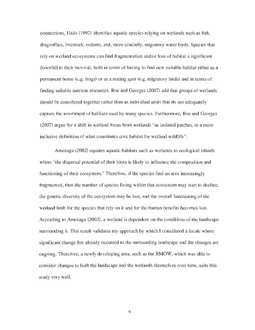
connections, Hails (1997) identifies aquatic species relying on wetlands such as fish,

dragonflies, livestock. rodents, and, more crucially, migratory water birds. Species that

rely on wetland ecosystems can find fragmentation and/or loss of habitat a significant

downfall to their survival, both in terms of having to find new suitable habitat either as a

permanent home (e.g. frogs) o r as a resting spot (e.g. migratory birds) and in terms of

finding suitable nutrient resources. Roe and Georges (2007) add that groups of wetlands

should be considered together rather than as individual units that do not adequately

capture the assortment of habitats used by many species. Furthermore, Roe and Georges

(2007) argue for a shift in wetland focus from wetlands "as isolated patches, to a more

inclusive definition of what constitutes core habitat for wetland wildlife".

Amezaga (2002) equates aquatic habitats such as wetlands to ecological islands

where "the dispersal potential of their biota is likely to influence the composition and

functioning of their ecosystem." Therefore, if the species find an area increasingly

fragmented, then the number of species living within that ecosystem may start to decline,

the genetic diversity of the ecosystem may be lost, and the overall functioning of the

wetland both for the species that rely on it and for the human benefits becomes lost.

According to Amezaga (2002). a wetland is dependent on the conditions of the landscape

surrounding it. This result validates my approach by which I considered a locale where

significant change has already occurred to the surrounding landscape and the changes are

ongoing. Therefore, a newly developing area, such as the RMOW, which was able to

consider changes to both the landscape and the wetlands themselves over time, suits this

study very well.

While most wetland ecosystem research has concentrated on hydrology,

composition, and species diversity, this study focused on fragmentation, connectivity, and

habitat loss. Throughout my literature review, I examined numerous papers, but only a

few dealt with fragmentation, connectivity, and habitat loss (Lehtinen et al 1999,

Amezaga et a1 2002, Leibowitz and Vining 2003, Yue et al2004, Roe and Georges

2007). In particular, the identification of wetland ecosystems from aerial photographs

was of interest because it related directly to data creation methods required for this study.

Papers identifying applicable techniques were difficult to find. Some, such as

Konstantinov 1997, Pavri and Aber 2004, Parmuchi et al2002, Ozemi and Bauer 2002,

Janssen et al 2005, Cox 1992, identified different ecosystems and the range of techniques

involved for identification of extent and pattern on the landscape. These subsequently

provided a basis from which suitable methods were designed.

2.3 Study Area

Located 120 kilometres north of Vancouver, British Columbia, the Resort

Municipality of Whistler (RMOW) is bordered by the Coast Mountains on the east and

west and is bisected by a highway travelling in a north-south direction along the valley

bottom (Figure 3). As the first municipality in the world to have been officially named a

resort municipality, the RMOW is co-host to the 2010 Olympics. Whistler, noted for its

outdoor recreation activity located on Blackcomb and Whistler Mountain, provides

opportunities for diverse activities in the winter and summer months.

r igure 5 : wuay aite: I ne Kesorr lwunicipality or w nistrer, rrrinsn corumbia, Canada.

The study was restricted to areas at an elevation of less than 1000 meters within

the municipal boundary of the Resort Municipality of Whistler. As most wetlands were

found along drainage channels and at lower elevations where water can pool and

stagnate, this was an acceptable limit to the study area that made the required data

analysis feasible within the time allowed. Another reason for bounding the study area by

elevation was to allow the focus to be on the changes found within the RMOW due to

urban development, which was concentrated at lower elevations throughout the valley

bottom with the exception of both Whistler and Blackcomb Mountains. In addition, the

amount of available data influenced this decision. Because most data focused on the

valley portion of the RMOW, where most of the development was located and where

most of the wetlands in 2003 occurred, this bounding was extremely useful.

Anthropogenic changes to the landscape in the RMOW began in 1914 during the

construction of the railway and continued with increasing intensity. Lodges began to

open throughout lower elevations in the 1950s primarily to facilitate access for the

abundant fish stocks found in the local area. In 1966, Whistler officially opened for

skiing after the completion of the first major road in 1965. Construction began on the new

town centre in 1978 and Blackcomb Mountain opened in 1980 making the Resort

Municipality of Whistler one of the largest ski complexes in North America. From then

on Whistler continued to develop, expand, and become an ever more important part of the

recreational side of life on the coast of British Columbia.

In 1999, the Resort Municipality of Whistler (RMOW) created the Whistler

Environmental Strategy, which set up the RMOW protected areas network steering

committee. The strategy outlined the formation of a Protected Area Network (PAN),

which guides the RMOW "to protect key remaining natural and semi-natural areas in the

Whistler valley within municipal boundaries" (Whistler Environmental strategy2 1999).

The PAN focuses awareness on unique and sensitive habitats throughout the municipality

including wetlands, riparian areas, old growth forests. and the ecological corridors that

connect these areas.

The RMOW PAN uses three levels of ecosystem protection: key protected areas,

special management zones, and reserve lands. Key protected areas are those areas

protected from any human development except low impact trails, boardwalks, or wildlife

viewing platforms. Special management zones are areas where only low impact human

development can occur such as nature trails. Reserve lands are large areas of relatively

Information pertaining to the Protected Area Network throughout Whistler come from Whistler's Environmental Strategy

natural land that allow for development o r recreational activities as long as an

environmental impact assessment is completed beforehand.

The PAN sets out goals and targets for the RMOW allowing for non-legislated

protection of the local ecosystems. The suggested target is to protect 100% of ecosystems

found within the municipal boundaries in 2006. However, this target yields various

considerations, in particular the question that led to this study: If 100% of the ecosystems

present in 2006 were protected, how much of a given ecosystem was lost in preceding

years.

3 METHODS

3.1 Data Collection

A substantial amount of data was required for this study including wetland

boundaries, water surfaces (major such as lakes and minor such as small streams),

railway, highway, elevation. slope, development footprint at each time step, and any

other data available associated with the RMOW terrain. As both wetland boundaries and

the development footprint are time sensitive, their extent depended on the changes that

occurred throughout Whistler at a given moment in time. Readily available data, provided

from within the RMOW, was combined with data created using aerial photographs of

different time steps.

3.1.1 Existing Data

The RMOW provided a substantial amount of digital data including aerial

photographs for 2003, elevation layers, and terrain ecosystem mapping (TEM) done by

Blackwell and Associates for the RMOW towards the end of 2003. Other data sets

provided include railway, highway, slope, water (both minor and major), and municipal

boundary. Together these data sources provided much of the base information necessary

to obtain a detailed idea of what the 2003 situation was in Whistler, not only for

wetlands, but also for a variety of ecosystems found throughout the region and within the

boundaries of the municipality.

3.1.2 Aerial Photograph Selection

Data showing the extent of wetland ecosystems and the changes to the

development footprint at various time steps were not available. Instead, these were

derived from an analysis of historical aerial photographs. Availability of data and

representativeness of development stages of the RMOW were the primary selection

criteria used to choose a useful, acceptable, and comprehensive set of aerial photographs

for the study. Selected historical aerial photographs were purchased from the Ministry of

Sustainable Resources: Base Mapping and Geomatics Services. Recent aerial

photographs were acquired through the RMOW as they are currently in use by the

municipality. Aerial photographs ordered through the Ministry of Sustainable Resources

were bought as diapositive images on 10x10 sheets allowing for a clearly visible image.

Diaposit ives are transparent positive images made on plastic-based emulsions. Lillisand

and Kiefer (2000) explain that a positive image refers to the regular processing and

exposure of film generating a negative of reversed scene geometry and brightness. The

film was then placed in emulsion-to-emulsion contact where light was passed through the

negative, exposing the paper creating a positive representation of the original image seen

on the ground. Each year selected had a range of photographs available and those

selected were all in black and white taken during the spring or summer months Lo avoid

snow covered images. This material is presented in detail in Table 1. The images selected

follow the valley bottom primarily and cover portions of two major stream channels

found within the RMOW, Fitzsimmons Creek and Callaghan Creek.

Table 1: Aerial photograph specifics bought from the Ministry of Sustainable Resources for study years 1946, 1969, and 1982 of the Resort Municipality of Whistler. Please note that 2003 data was not purchased as it was made available by the RMOW.

I Date Flown 1 Scale 1 # of Images I Roll Number I 1 1946 1 n/a 1 l:4O chains 1 16 / BC262 / 1 1969 1 June 4 1 1:16000 1 30 1 15BC5333 1

I I I I

1982 1 Sept. 18 1 1:20 000 / 24 1 30BC82062

The year 1946 was the starting point for the study since it was the first complete

available aerial photograph record. Prior to 1946, forest survey records and railway notes

exist; however, these are less reliable than aerial photographs because interpretations of

the area was based on surveyors recording what was seen at the time on the ground while

aerial photographs provided an image that allowed for individual interpretation with

today's knowledge with less subjectivity in site interpretation. Therefore, forest survey

records and railway notes were not used in this study. The year 1946 represents the

RMOW post railway development, post building of Rainbow Lodge primarily for fishing,

and was before highway construction began.

The year 1969 marks a couple of years following the opening of Whistler

Mountain in 1 9 6 6 ~ ouris ism Whistler) and the construction of the highway, completed

between 1965 and 1966. This moment in time was before the development of Whistler

Village and Blackcomb Mountain.

The late 70s and the early 80s saw the completion of the initial Whistler Village

development and the opening of Blackcomb Mountain. Both developments were critical

in forming the Whistler seen in 2003 because the combination of Blackcomb and

i Information on the specific history of the RMOW was collected from Tourism Whistler's Chronological History

Whistler Mountain provide one of the largest outdoor recreation resorts in North America

while Whistler Village provides the centre point for activities throughout the RMOW.

The next aerial photograph selection was from 1982, documenting the region before

development soared in the nineties.

Development throughout the nineties was rapid, both in terms of urban area

construction throughout the RMOW and with the types of activities commonly found

throughout Whistler. Prior to the mid-90s, Whistler was known for its ski hills and resort

village; however, throughout the 90s more emphasis was placed on expanding the

summer activities in the region, particularly mountain biking on the ski hills. The final

aerial photograph selection was from 2003, showing some of the major changes that

increased development had on the region.

3.2 Data Creation

3.2.1 Aerial Photograph Interpretation

Prior to interpretation, each diapositive aerial photograph was scanned at a

resolution of 1600 dpi and was saved as a t i ff (tagged image file format). The scanned

images were printed at high resolution on high quality paper and laminated. Various

methods for aerial photograph interpretation exist including manual interpretation using a

mirror stereoscope to unsupervised or supervised classification methods done on the

computer. After a thorough literature review of methods used to interpret aerial

photographs, a general theme was that aerial photograph interpretations capture the

landscape at one instant and result in high levels of site-specific information (Cox 1992)

while computer based methods either using satellite imagery or aerial photographs were

problematic and had limitations (Ozemi and Bauer 2002, Cox 1992). Although

supervised and unsupervised classifications are good options, they were unlikely to

provide the accuracy desired for the project. Therefore, manual interpretation methods

were used. For the purposes of this study, one person completed image interpretation

(using a mirror stereoscope) to maintain consistency in the interpretations (Figure 4). For

each set of images, the boundaries of the wetland ecosystems were delineated as well as

the major water bodies, the railway, the highway, and any development footprint visible

at each temporal interval.

r lgure 4: Image interpretation us111g 11111-1-01- SLCI-CUSCU~C

The wetland ecosystem boundaries were of most importance since they were the

basis for this study. In order to determine which areas were wetlands, a list of various

types of areas to search for was created including

Areas known in 2003 to have wetlands.

Areas along drainage lines.

Areas in low lying elevations,

Areas with extensive exposed soils.

Although not all wetland boundaries were immediately recognisable, with time and

repetition the wetlands become more apparent. Interpretation began with the 2003

images, where I already had delineated wetland polygons. Prior to evaluating existing

wetland polygons, I interpreted the 2003 images and then compared my interpretation

with those provided in the TEM by B.A. Blackwell and Associates (2004). The TEM

wetlands and those interpreted were very close. Using this comparison, I was able to

pseudo-field check my data because I was comparing with the known wetlands in the

TEM, which had been field checked, providing an accurate check for myself. Throughout

interpretations. I revisited earlier image interpretations to ensure that my analysis was

complete and that each image had the same basis for interpretation. In a few cases, I had

some questionable wetlands and in those instances because there was never more than

one for any time-period, they were omitted from the final analysis.

Delineating boundaries around areas of urban development created the

development footprint for each time step. Areas that appeared built up including houses

and buildings were considered part of the development footprint. Some areas appeared to

be under construction at the date of the aerial photograph and if they were only in the

beginning stages where there were no buildings on the property then they were not

considered part of the development footprint at that time step.

By delineating the highway, railway, and major water bodies, I was able not only

to determine the orientation of the overlays for continued interpretation, but in particular

for input into digital data and proper orientation to existing data. The railway and the

highway allowed me to determine where the interpretation fit among existing digital data,

therefore providing a key reference point. Conversely, since water bodies are likely to

change over time, particularly the water levels. they offered limited suitability for

determining the geographical location of the images.

3.2.2 Digitizing the Data

Upon completion of the aerial photograph interpretation. the delineated images

were digitized in order to run a variety of connectivity analyses on the data (Figure 5).

Each image was scanned at 70 dpi (dots per inch) in order to maintain a reasonable

resolution without creating extremely large file sizes. The images were cropped, rotated if

necessary, and brought into ER Mapper to save as raster datasets. The images were

warped individually according to an existing georeferenced dataset then tiled together to

create one large image for each year of data.

of wetlands (orange) and deve lph and digitized aerial photograph il ,nt footprint (purple) for the RMOW

nterpretation in 2003.

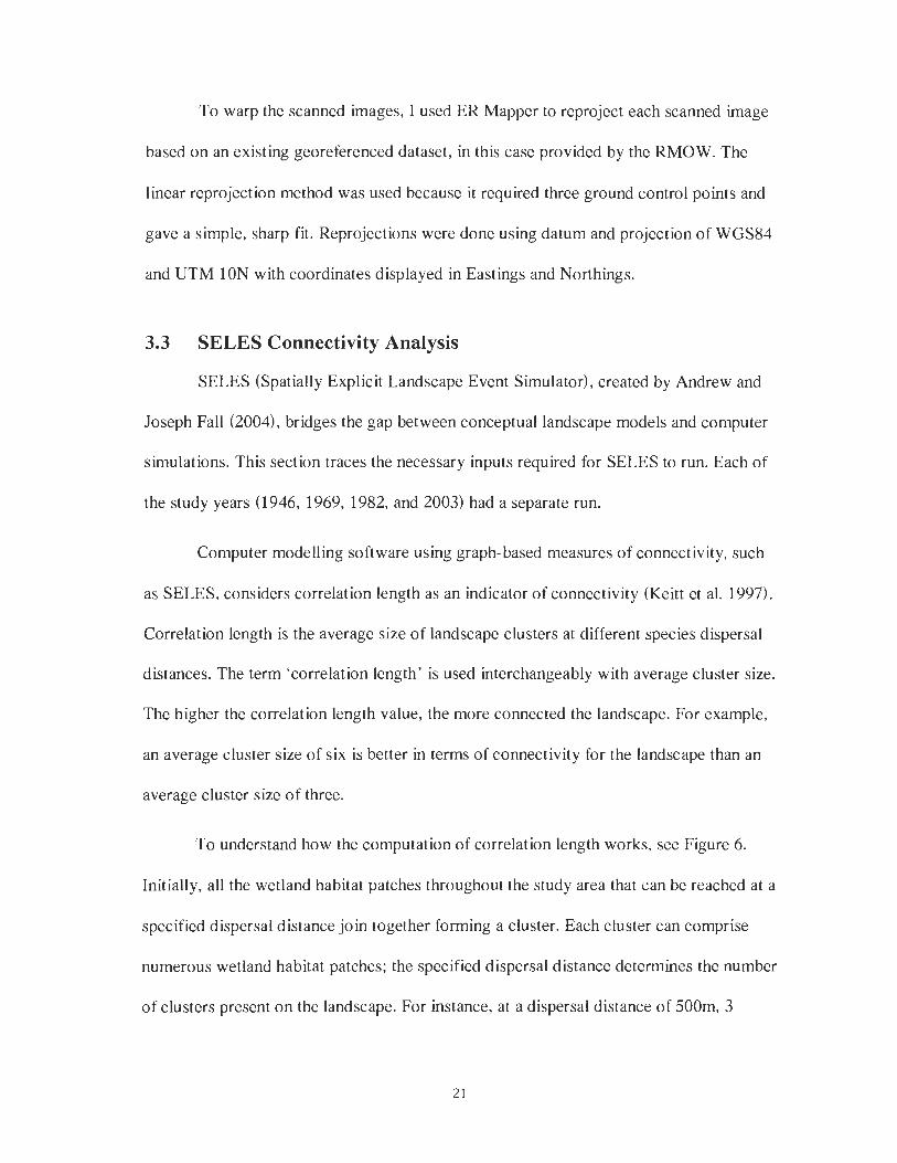
To warp the scanned images, I used ER Mapper to reproject each scanned image

based on an existing georeferenced dataset, in this case provided by the RMOW. The

linear reprojection method was used because it required three ground control points and

gave a simple, sharp fit. Reprojections were done using datum and projection of WGS84

and UTM 10N with coordinates displayed in East ings and Northings.

3.3 SELES Connectivity Analysis

SELES (Spatially Explicit Landscape Event Simulator), created by Andrew and

Joseph Fall (2004). bridges the gap between conceptual landscape models and computer

simulations. This section traces the necessary inputs required for SELES to run. Each of

the study years (1946, 1969, 1982, and 2003) had a separate run.

Computer modelling software using graph-based measures of connectivity, such

as SELES, considers correlation length as an indicator of connectivity (Keitt et al. 1997).

Correlation length is the average size of landscape clusters at different species dispersal

distances. The term 'correlation length' is used interchangeably with average cluster size.

The higher the correlation length value, the more connected the landscape. For example,

an average cluster size of six is better in terms of connectivity for the landscape than an

average cluster size of three.

To understand how the computation of correlation length works, see Figure 6.

Initially, all the wetland habitat patches throughout the study area that can be reached at a

specified dispersal distance join together forming a cluster. Each cluster can comprise

numerous wetland habitat patches; the specified dispersal distance determines the number

of clusters present on the landscape. For instance, at a dispersal distance of 500m, 3

separate clusters on the landscape comprising between 3 and 5 wetland habitat patches

are distinguished. This process is then repeated for different species dispersal distances at

specified intervals. For clarification, when SELES conducts an analysis. habitat patches

were considered from edge to edge, not from centre to centre. If the interval increases by

500m to a species dispersal distance of 1000m. there may only be 2 clusters on the

landscape, each of which comprises between 5 and 10 wetland habitat patches. These

changes become apparent since areas that were unreachable at a dispersal distance of

500m are now reachable at a dispersal distance of 1000m and therefore were considered

by SELES to be one patch. If the process continues and the interval was repeated again,

the next result might identify only one cluster at a species dispersal distance of 1500m

where the cluster is comprised of all wetland habitat patches on the landscape. SELES

correlation length statistics report the average cluster size at each specified species

dispersal distance and the intervals at which the calculations are computed depend on the

analysis design.

Figure 6: Depiction of how SELES determines average cluster size. (A) Three clusters of habitat patches are connected a t a threshold distance of 500111 (B) Two clusters of habitat patches connected a t a threshold distance of 1000m, note the line joining the two original clusters (C) One cluster of habitat patches connected a t a threshold distance of 2000m. note the lines connecting all three original clusters.

3.3.1 Analysis Extent

SELES requires a file that defines the analysis extent. Since I was working with

grid files, the easiest way to define the analysis extent was by using a rectangle that could

be common throughout all layers required by SELES. The analysis extent remained

standard throughout the study. Also of note, the study area grid had a spatial resolution of

25m x 25m cell size in order to achieve as much detail as possible for the circumstances

of the study.

3.3.2 Wetland (Habitat Patch) Surface

The wetland layers, digitized from aerial photograph interpretations, were

buffered by 25m to remove any cracks and to make sure no unnatural breaks were

created. Cracks result when narrow land features that are costly to species (such as a

railway) are represented in raster form and "lead to erroneous identification of non-

existent shortcuts across truly expensive barriers" (Rothley 2005). For example, as

presented in Figure 7, converting the railway to raster form without the use of a buffer

resulted in the presence of 'cracks'.

I I Figure 7: Conversion of railway from a vector file (brown) to a raster grid (blue) resulting in the creation of 'cracks'.

The wetland layers were defined in terms of zeros and ones where a zero was

considered non-habitat and one was considered habitat. Once the values were set, the

wetland layers were converted into raster grids based on the analysis extent and exported

as an ASCII Raster data format to be used in SELES and later with Patch Analyst in

ArcView (Environmental Systems Research Institute 2000). As wetland habitat surface

varied by year (1946, 1969, 1982, and 2003) and although the number of patches in a

given year may be the same as the patches in another year, they may not be the same

habitat patches.

Calculating Resistance Surfaces

SELES requires resistance surfaces (also known as cost surfaces) in order to

determine the travel cost associated with an organism moving across the landscape

between wetland patches. The analysis design identified overall trends throughout the

RMOW, without considering a focal species. As a result, general resistance surfaces that

applied to all species supported the identification of overall trends. Initially, the intent

was to create resistance surfaces based on land cover types found within the TEM

provided by the RMOW. However, reconstructing the landscape in terms of forest,

wetlands, and other land cover types in sites either harvested or developed between 1946

and 2003, was extremely difficult for a number of reasons. First, since no record of land

cover was present prior to 1946, there was no method to account accurately for previous

land cover in sites developed in 1946. Second, the amount of detail covered by the TEM

was substantial and in order to re-create the same level o f detail for all prior years, would

have required significant amounts of research and would still likely have yielded results

that were inaccurate. Last, in order to reconstruct an accurate landscape for each time-

period, the time required would have exceeded that which was possible for this project. In

order to reconstruct the landscape properly, a substantial amount of time, a significant

amount of research, and a good eye for detail would have been necessary. Due to these

reasons, it was unlikely that reconstruction of the landscape would yield accurate land

cover for each time step to an acceptable level of detail. Therefore. I assumed that travel

cost was a function of the percent slope, water, railway, highway, and development

footprint at each time. The inputs to the travel cost function were selected because they

represent the landscape in as much detail as was available for the years of the study.

The primary concern of this study was to determine changes to wetland

ecosystems and although some minimal changes may have occurred in other ecosystems

throughout the region. the primary and most noticeable changes occurred within the

development footprint. The focus of the travel cost was on development, which included

railway and highway as well as natural features such as percent slope and water. High

resistance values were given to areas considered difficult for species to travel through.

For example, railways, which intrude on the natural landscape, result in increased risk of

mortality. Low resistance values were given to areas considered relatively easy to pass

through from a species point of view. For example, wetland species are unlikely to find

water a daunting passage in terms of travel cost because they thrive in semi-aquatic

landscape. Each of the necessary portions of the overall resistance surface was created in

ArcView 3.3 using the Spatial Analyst Extension (the details of which are in the

following sect ions).

3.3.3.1 Slope

The slope layer was created from 20m contour TRIM data provided by the

RMOW. The pits in the data were filled and then in ArcView the slope function was used

to calculate the percent slope. Pits are areas of abnormality created through interpolation

of data that can result in inaccurate results from misrepresentation of depressions

occurring in narrow valleys, at all resolutions as well as areas of gentle relief (Burrough

and McDonnell, 1998). To account for this problem, identification of pits was necessary.

Once all pits were found, an evaluation of the neighbour cells was completed to

determine what value the cell would be assigned, essentially increasing the elevation until

it was equal to one or more of its neighbour cells and then examining the surrounding

grid cells to make sure the pit was not part of the true elevation.

The slope layer was the base layer for creating the resistance surfaces. The slope

layer ranged in values from 1 to 62 where areas of high slope were 62 and areas of low

slope were 1. The value of 62 was the percent slope value for areas considered extremely

difficult for species to travel through. For example, most species are likely to travel

through the paths of least resistance therefore making high slope areas unlikely targets for

travel corridors and, conversely, flat areas favoured travel corridors (Singleton et al.

2002)

3.3.3.2 Water

For the effects of water on travel between wetlands, I assumed that the 2003

watercourses were a reasonable surrogate for the general location of watercourses within

and between wetlands for all time-periods (1946-2003). In order to create this layer, I

took existing water data in shape files format, buffered the polygons by 25m, then

converted the dataset to a raster grid using analysis extent as a basis. Therefore, buffering

the water ensured that the watercourses were not divided by breaks created by rasterizing

the file and that the watercourses were not susceptible to any problems with "cracks". In

this case, the water received a value of 12 cost units, amounting to 20% of the highest

cost value in the slope layer. The reason for this was to make the water passable, but not

the first choice if a lower percent slope travel corridor was nearby.

3.3.3.3 Railway

Buffering the railway surface by 25m removed any cracks and ensured unnatural

breaks remained absent. The railway received a cost value of 62, the highest cost value

associated with the slope layer while all other areas had a value of 0. Once reclassified

and the values set, the railway was converted to a raster grid based on analysis extent.

3.3.3.4 Highway

A 25-meter buffer around the highway surface avoided the generation of any

cracks and ensured that unnatural breaks did not exist. A cost value of 62, the highest

value available in the study, was assigned to the highway layer because it was considered

as a barrier on the landscape, which species would avoid given natural alternatives. Once

reclassified and the values set, the highway was converted to a raster grid based on

analysis extent.

3.3.3.5 Development Footprint

Based on aerial photograph interpretations, the development footprint identified

the areas of urban development throughout the RMOW including roads, households,

industrial areas, golf courses, and construction sites. Each study year (1969, 1982, and

2003) required a development footprint. However, in the 1946 imagery there were no

visible signs of development; therefore, no development footprint was necessary in the

analysis of the 1946 wetland extent. Each development footprint created showed

substantial change to urban growth throughout the RMOW and was accounted for

accordingly in the study.

Each development footprint surface was buffered by 25m in order to remove any

cracks and to make sure unnatural breaks were not created. The development footprint

layers were given a cost value of 62, the highest cost value associated with the slope

layer. Once the values were set, the development footprint layers were converted to raster

grids based on analysis extent set.

3.3.3.6 RMOW and Elevation Mask

The mask bounds the study area by the municipal boundary of the Resort

Municipality of Whistler and by elevation less than 1000 meters. The mask was applied

at the end of the creation of the resistance surfaces in order to restrict movement within

the connectivity analysis to solely within the study region.

3.3.3.7 Burning In Layers to Create Final Resistance Surfaces

Burning in was a process of data integration where each of the layers was

combined. The layers formed a single resistance surface portraying the values from each

input layer. The slope layer was used as the base layer while water, railway, highway,

and development footprint were added by using the spatial analyst extension in ArcView

and calculating map statistics where the maximum value in each cell was selected. For

example, if a grid cell had a value of 6 in the slope layer, then in the water layer, the same

grid cell had a value of 12. Thus, 1 2 would be selected as the associated value with that

cell. The mask layer was added last to the resistance surface using ArcView where the

value of each grid cell in the mask was added to the layers already created. For example,

when the mask with a value of 6 2 was added to a grid cell having a value of 12, then the

grid cell was assigned an updated value of 74. The input layers associated with each

resistance surface are in Table 2 and the resistance layers are shown in Figure 8.

Table 2: Input layers associated with each resistance surface for each study year beginning in 1946 and ending in 2003.

Slope Water Railway Highway 1969 Develooment Footprint

I Boundary and Elevation Mask ( X X X X

X X X

1982 Development Footprint 2003 Develooment Footorint

(SELES uses ASCII files) for 1946 (teal), 1969 (Red), 1982 (Green), and 2003 (Blue).

X X

Running SELES

I ran two parts of SELES: graph extraction and graph analysis. Graph extraction

considers the input files, assigns unique identifications to the patches and calculates the

X X X

X

X

X

X X X

X

X X X

least cost path based on the resistance surfaces. Graph analysis calculates the correlation

length for the range and interval of dispersal distances provided by the user.

3.3.4.1 Graph Extraction

Graph extraction looks at the input files, creates unique IDS for the habitat

patches, considers the resistance surface, and then calculates the least cost path. Defining

various parameters occurred during the setup for graph extraction (Appendix A). Initially.

I could do the graph extraction using either the minimum planar graph or the complete

graph. The minimum planar graph connects all patches by at least one edge with no

crossover while the complete graph connects all pairs regardless of crossover. For the

purposes of this study, the complete graph showed all possible connections (Fall 2004)

giving a comprehensive result, thus showing a more complete, accurate depiction of the

landscape. Another important parameter to set was the patch size threshold, which

controls whether or not SELES disregarded patches that may have been too small. For the

study, all patches were important and therefore the patch size threshold was set at 0.0625

hectares (less than the smallest patch size so that all wetland patches would be included

as nodes in the analysis). A final parameter to establish prior to running this portion of

the model was to set the study area type. Three options were available: study area

defined, entire landscape, and computing a convex hull of original patches. Since, the

study area was already defined by analysis extent, study area defined was selected.

3.3.4.2 Graph Analysis

Graph analysis calculated the correlation length based on the files created in graph

extraction. A few parameters needed to be set during this process such as threshold

increment and number of thresholds (Appendix B). A threshold increment of 100 was

used to provide a clear range of dispersal distances and the number of thresholds was set

to a value slightly larger than the longest least cost path distance between the two farthest

patches to make sure that all possible connections among patches were found.

3.3.4.3 Run Variations

I conducted three sets of SELES runs. On the first run of the model, it was

important to let the model run to the defined specifications set above in sections 3.3.4.1

and 3.3.4.2 where all runs checked the wetland and the cost surface for a given year. In

this instance, the number of thresholds used in graph analysis was set to a value slightly

larger than the longest distance between patches, providing a complete result.

The second set of model runs considered the same wetland and cost surface for a

given year, but for comparative purposes restricted the threshold number to a value of

301 resulting in a calculation up to 30 000 meters to encompass the vast majority of

changes shown throughout the RMOW. A value of 301 was used because in comparison

between each set of results, the point at which each graph levels off and shows no more

change occurs at the latest by 30 000m. To ensure that the model runs to 30 OOOm, a

threshold number of 300 should be used; however, by adding one more to the total, the

model will run past 30 OOOm and will encompass as much of the data as necessary. The

reason for this was to exaggerate the detail in the model portion where the greatest

change was occurring. Thirty thousand meters was not decided arbitrarily; it was

approximately 95% of the total model output and was where most of the substantial

differences between years could be shown. Results for correlation length using a

straightforward approach were presented using this set of runs.

The third set of runs attempted to answer, 'Has the change in connectivity resulted

from changes in the wetland patches, changes in the matrix, or both?' from the research

questions. To do that, I held either the patches or the matrix for a given year constant

while varying the other. For example, for a comparison of the effect of changes between

1946 and 1969, I considered the original (1946 patches with 1946 matrix) then I

considered the 1946 patches with the 1969 matrix to determine if a matrix effect was

occurring and I looked at the 1946 matrix with the 1969 patches to determine if a patch

effect was occurring. I completed three comparisons looking at (1) the effect of the

highway between 1946 and 1969, (2) the effect of opening Blackcomb Mountain and

Whistler Village between 1969 and 1982. and (3) the effect of intense urban development

throughout the RMOW between 1982 and 2003. Table 3 provides the set up for each

comparison. The results for correlation length, a multifaceted approach, originated from

this set of model runs.

Table 3: Comparative Analysis to determine whether changes in connectivity over time are a result of a wetland habitat patch effect or a resistance surface matrix effect (red = effect of highway, green = effect of ski developments, blue = effect of urban development)

1946 patch

1969 matrix

1 2003 matrix I I I Matrix Effect I Original

1982 matrix

1969 patch

Matrix Effect

1946 matrix

Matrix Effect

0 _ tch Efl [

1982 patch

Original

2003 patch

Patch Effect

Original Patch Effect

3.3.5 Sensitivity Analysis

Adriaensen et a1 (2003) note, that regardless of the data source, sensitivity

analysis is worthwhile. Throughout the literature (Larkin et al. 2004, Verbeylen et al.

2003), the most controversial aspect of graph-based studies using resistance surfaces is

the values used for the surfaces. Therefore, testing the inputs was important to see if the

results and conclusions made from the data could be substantiated. Larkin et al. (2004)

along with Knaapen et al. (1992) suggested that by rescaling the resistance values used

for the resistance surface an understanding of the robustness of their model could be

shown. Verbeylen et al. (2003) presented another option where 36 different resistance

surfaces were generated and tested by changing the number of land-cover classes and

changing the resistance values. Sensitivity analysis allowed the quantification of the

effect of changing assumptions about the resistance scores (which were set largely

subjectively) and the buffer sizes. In the study, I used data sets from various sources;

however, the most important sensitivity analysis related directly to the resistance

surfaces. Sensitivity analysis on the buffers was used in the creation of the resistance

surfaces and on the resistance values used in the final surfaces following the methods of

Larkin et al. (2004) and Knaapen et al. (1992).

3.3.5.1 Buffers

The buffers used in the main analysis were set at 25m to represent accurately the

linear features once turned into a grid. Therefore, to determine how sensitive the analysis

was to the predefined buffer, I increased and decreased the buffer sizes by 20% and ran

the analysis using a 20m buffer and a 30m buffer to account for the extremes of

variability. Surfaces in the analysis that used a buffer included water, railway, highway,

and wetlands.

3.3.5.2 Resistance Values

A sensitivity analysis of the resistance values was completed in order to provide a

clear understanding of the effect of the resistance surface and the associated values. For

this study, I rescaled the values of the resistance values to minimize or maximize results,

then compared the proportion of overlap to the original to determine if, in fact, the initial

resistance surface provided a relatively accurate representation of the real world (Larkin

et al. 2004 and Knaapen et al. 1992). The other option for considering resistance surfaces

was to vary the resistance values and the land cover classes as shown by Verbeylen et a1

(2003) with 36 different resistance layers. However, due to scope, this was not feasible

because in order to create 36 different resistance layers for each time step and run the

variations would require a substantial amount of time. Because of the temporal scale used

throughout this study, an option such as that shown by Larkin et al. (2004) and Knaapen

et a1 (1992) was more suitable.

The resistance values were rescaled from 1 to 62 down to 1 to 31 and up to 1 to

93. Each shift was altered by a value of 31 up or down from the original analysis values

selected. This ensured that comparison of the changes could be undertaken.

3.4 Common Connectivity Metrics Analysis

Consideration of various common connectivity metrics was required to answer the

fourth question 'How does my assessment of connectivity change when using the

standard measures of connectivity (patch size, area, total edges) versus using graph-based

metrics?' Common connectivity metrics include, but are not limited to, patch measures

such as size, shape, perimeter, orientation, and perimeter: area ratio, and mosaic measures

including patch number, edge density, fractal dimension, and patch size frequency

distribution (Gutzwiller 2002). When connectivity studies first made their way into

academic literature, the methods used to describe the degree of fragmentation within a

given study region focused on the landscape structure using statistical measures that were

easily calculated. These measures, although they provide information on the landscape,

do not consider the idea of corridors and connected landscapes by considering paths used

by species. By considering solely the habitat and the measures of the habitat itself, some

of the direct impacts by the loss in connectivity to the species themselves likely were

missed.

To calculate various common connectivity metrics. I used the Patch Analyst for

grids extension in ArcView 3.3 where I calculated spatial statistics using the Fragstats

interface. I calculated a variety of metrics, but for those used for considering connectivity

I chose only the following: class area, mean patch size, total edge, mean shape index,

mean patch fractal dimension, total core area, and mean core area.

In order to run spatial statistics calculations, the wetland patches had to be in

raster format. To do this, I used the wetland habitat patches digitized from aerial

photograph interpretations, buffered them by 25m to remove any cracks and to ensure no

unnatural breaks were created. Next, the layer was defined in terms of 0s and I s where 0

was considered non-habitat and 1 was considered habitat (same surfaces as used in

SELES). Then the layer was converted to raster format and used as the input with the

patch analyst extension.

4 RESULTS

4.1 Correlation Length: Straightforward Comparison

As the focus of the study was on overall trends, initial analysis using SELES

considered correlation length as a function of numerous species dispersal distances.

Correlation length is the average size of landscape clusters at different species dispersal

capabilities (threshold distances). The higher the correlation length value, the more

connected the landscape.

All graphs portray average cluster size (also known as correlation length) on the

y-axis with species dispersal capability (also known as threshold distance) on the x-axis.

In this analysis, I considered habitat patches from each of the study years and ran SELES

according to the resistance surface associated with each year. The matrix refers to the

grid cells associated with the resistance surface and, in particular, the values associated

with those grid cells. Each value represents a particular detail of the landscape creating a

matrix to represent the overall landscape.

For ease of understanding and comparison, I consider two fictional example

species throughout the results. The first example is 'Species A' which has a maximum

dispersal distance of 10 OOOm and the second example is 'Species B' which has a

maximum dispersal distance of 15 000m. Throughout the results when considering the

graphs and the results, the landscape changes from the point of view of 'Species A' and

'Species B' provide the focus.

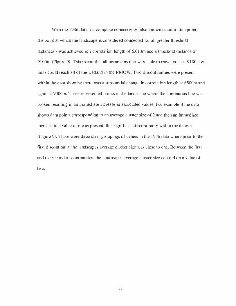
With the 1946 data set, complete connectivity (also known as saturation point) -

the point at which the landscape is considered connected for all greater threshold

distances - was achieved at a correlation length of 6.01 3m and a threshold distance of

9100m (Figure 9). This meant that all organisms that were able to travel at least 9100 cost

units could reach all of the wetland in the RMOW. Two discontinuities were present

within the data showing there was a substantial change in correlation length at 6500m and

again at 9000m. These represented points in the landscape where the continuous line was

broken resulting in an immediate increase in associated values. For example if the data

shows data points corresponding to an average cluster size of 2 and then an immediate

increase to a value of 6 was present, this signifies a discontinuity within the dataset

(Figure 9). There were three clear groupings of values in the 1946 data where prior to the

first discontinuity the landscapes average cluster size was close to one. Between the first

and the second discontinuities, the landscapes average cluster size centred on a value of

two.

Species Dispersal Distance (meters)

Figure 9: Results for the year 1946 showing complete connectivity at a dispersal distance of 9100m and an average cluster size of 6.013m.

To understand further the results from 1946, consider 'Species A' with a dispersal

distance of 10 OOOm and 'Species B' with a dispersal distance of 15 000m. In 1946, they

both found the landscape completely connected meaning that they could move between

all wetland patches within the RMOW with relative ease. They were not hindered,

restricted, nor limited to certain patches.

The 1969 data curve was added to the 1946 graph for comparison purposes

(Figure 10). In 1969, the point at which the landscape was considered completely

connected was found at an average cluster size of 4.353m and a threshold distance of

12700m. The discontinuities shown in the 1946 data were still present in the 1969 data;

however, they were markedly smaller. In particular, the first discontinuity occurred at

10100m and concentrated on an average cluster size value of 1.263m. The second

discontinuity occurred at 12600m and focused on average cluster size values close to

1.622m. Three groupings of data points were still present.

Species Dispersal Distance (meters)

Figure 10: Results for the year 1969 and 1946 where in 1969 complete connectivity is reached at a dispersal distance of 12700m and attains an average cluster size of 4.353m.

Consider 'Species A' which disperses at a distance of 10 000m. In 1969, it found

that the amount of suitable habitat it could reach had reduced substantially from 1946.

For this species, the landscape in 1969 was restricted as much as it would have been in

1946 for a 5000m disperser. 'Species B', whose maximum dispersal distance is 15 000m.

still found the landscape connected in 1969; however, 'Species B's ' overall connectivity

of the region decreased. In 1946 a level of 6.013m was reached; now only a level of

4.353m was achieved. It could still find all wetland habitat patches throughout the region

and was not restricted, as was the case with 'Species A' at the second time step.

For the 1982 data, complete connectivity was reached at an average cluster size of

3.305m and a threshold of 12300m (Figure 11). The 12300m was a shift from that of

1969 where the maximum average cluster size was reached at a threshold of 12700m.

However, the average cluster size between 1946 and 1982 decreased by 24.1%. The two

discontinuities were still present although the first discontinuity was becoming less

distinguished as it remained at a threshold value of 11 lOOm and an average cluster size

high of 1.362m. The second discontinuity was smaller again showing an average cluster

size of 1.633m at a threshold distance of 11800m.

7

- = s . - p - .- .- I

8 C

g 5 . -

r 0

T -

- - - - T T I I

0 5900 10000 15900 20000 25000 30000 35000

Species Dispersal Distance (meters)

Figure 11: Results for the year 1982 with those from 1946 and 1969 where in 1982 average cluster size reaches a maximum of 3.305m at a dispersal distance of 123UOm.

Returning to 'Species A', which has a dispersal distance of 10 000m. in 1982, it

found that there was no change in how much habitat it could reach from 1969. Therefore,

the same wetland habitats were still available to it. 'Species B' still found the RMOW

completely connected in 1982; however, it experienced continued decreases to the

average cluster sizes that it could find. It can now only find average cluster sizes of

3.305m throughout the municipality.

In 2003, complete connectivity occurred at a threshold distance of 26400m and an

average cluster size of 3.359m (see Figure 12). The maximum average cluster size seen in

2003 was close to that of 1982. The year 2003, still showed the two discontinuities. The

first occurred at a threshold distance of 20400m and an average cluster size of 1.235m

while the second discontinuity occurred at a threshold distance of 26300 m and had an

average cluster size of 1.726m. The three primary clusters seen in earlier years were not

present in 2003. The results from the year 2003 represent between 4 and 5 clusters of

data, which was a different pattern from that shown in previous years.

Species Dispersal Distance (meters)

Figure 12: Results for all years including 2003 as well as 1946, 1969. and 1982 where in 2003 average cluster size reached a maximum of 3.359m at a dispersal distance of 26400m.

From 'Species A's' point of view, the landscape had not changed again with a

dispersal distance of 10 000m. It was still seeing the landscape in the same manner in

1982 and in 1969, as it is able to reach the same suitable wetland habitats. For 'Species

B', which is restricted to a maximum dispersal distance of 15 OOOm, the 2003 landscape

revealed a complete change in its view of connectivity. The species no longer could reach

all the suitable habitat patches throughout the RMOW and its overall view of average

cluster size decreased to 1.168m.

4.2 Correlation Length: Multifaceted Comparison

The multifaceted comparison considered whether changes in connectivity

between time-periods were mainly the result of a matrix or a patch effect. In a matrix

effect, I was considering the possibility that the resistance surfaces had an effect on the

correlation length throughout the RMOW, while with a patch effect, I was looking to see

if the wetland habitat patches themselves resulted in changes in correlation length

throughout the study site. The primary points of comparison between a patch effect and a

matrix effect are the changes in species dispersal distances along the x-axis and the

average size of clusters shown along the y-axis

The first comparison considered the effect the implementation of the highway had

for connectivity in the RMOW. Figure 13 depicts the original data having an average

cluster size of 6.013m, which occurred at a dispersal distance of 9100m. This data set

also showed three clearly visible clusters and two discontinuities. The matrix effect,

which held the 1946 patches constant, but used the year 1969 matrix, showed an average

cluster size of 6.013m occurring at a dispersal distance of 11800m and clearly portrayed

three clusters of data and two discontinuities within the data. The patch effect that held

the 1946 matrix constant and used the 1969 patches displayed an average cluster size of

4.353m happening at a species dispersal distance of 12700m. The patch effect line

showed two clear clusters and one discontinuity.

0 5000 10000 15000 20000 25000 30000 35000

Species Dispersal Distance (meters)

Figure 13: Results comparing 1946 and 1969 when the highway construction bisected the RMOW valley. The matrix effect had minimal impact while the patch effect showed a decrease in the maximum average cluster size and pushed species with lower dispersal capabilities into smaller. more fragmented habitats.

The second comparison looked at the effect the ski development and the opening

of Whistler Village had for the connectivity of the RMOW. Figure 14 presented the

original data having an average cluster size of 4.353m, which occurred at a dispersal

distance of 12700m. This data set also showed two clusters and one large discontinuity.

The matrix effect, which held the 1969 patches constant, but used the 1982 matrix,

showed an average cluster size of 4.353m occurring at a dispersal distance of 12700m

and clearly portrayed two clusters and one large discontinuity. The patch effect that held

the 1969 matrix constant and used the 1982 patches displays an average cluster size of

3.272m happening at a species dispersal distance of 1 l9OOm. The patch effect line

showed two clusters and one discontinuity.

+Original

+Matrix Effect

0 5000 10000 15000 20000 25000 30000 35000 I Species Dispersal Distance (meters) I

1

Figure 14: Results comparing 1969 and 1982 when the ski developments (Whistler and Blackcomb Mountain) opened in the RMOW. The matrix effect had no impact while the patch effect showed a decrease in the maximum average cluster size.

The final comparison showed the effect intense urban development had

throughout Whistler Village on connectivity. Figure 15 shows the original data had an

average cluster size of 3.305m. which occurred at a dispersal distance of 12300m. This

data set also showed some clustering and one discontinuity. The matrix effect, which held

the 1982 patches constant, but used the 2003 matrix, showed an average cluster size of

3.271m occurring at a dispersal distance of 14800m and showed some clustering and one

discontinuity within the data. The patch effect that held the 1982 matrix constant and

used the 2003 patches displayed an average cluster size of 3.359m occurring for a species

dispersal distance of 24800m.

0 5000 10000 15000 20000 25000 30000 35000

Species Dispersal Distance (meters)

Figure 15: Results comparing 1982 and 2003 when the majority of urban development occurred throughout the RMOW. The matrix effect had minimal impact while the patch effect showed a similar maximum average cluster size, but the substantial changes occurred to species with dispersal capabilities between 12300m and 26400m.

4.3 Sensitivity Analysis

A large area of concern over the inputs applied to this analysis was in the

resistance surfaces used in the SELES runs for determining correlation length. Two

parameters were tested (1) the size of the buffer was varied by 20% to a buffer size of

20m and 30m and (2) the resistance values were re-scaled from an original scale of 1 to

62 to new values of 1 to 31 and 1 to 93. In this case. the values were varied by 31 both up

and down from the original because 31 was half of the original and could be used for

comparison of results later.

The first two sensitivity analyses considered variations occurring because of the

selection of a different buffer size. Figure 16 shows the curves generated using SELES

for 1946, 1969, 1982, and 2003 using a buffer of 20m, a 20% decrease from that used in

the original analyses. In this first graph, each year was evaluated individually using the

patches and matrix from the same year. For 1946, the maximum average cluster size was

5.896m occurring at a value of 8900m. In 1969, the highest average cluster size was

4.323m at a species dispersal capability of 11400m. For 1982, the largest average cluster

size was 3.30m happening at a dispersal value of 12000m. In 2003, the strongest average

cluster size was 3.359m experienced at a species dispersal capability of 25100m. Each

year showed a discontinuity leading up to the maximum average cluster size as well as

some clustering within the data similar to the original results shown in Figure 12.

5000 10000 15000 20000 25000 30000 35000

Species Dispersal Capability (meters) - -

Figure 16: Results comparing each study year 1946. 1969. 1982, and 2003 where the resistance surface matrix had a buffer size of 20 meters.

The second buffer sensitivity analysis increased the buffer size by 20% up to 30m

(Figure 17). For 1946, complete connectivity was reached at a species dispersal distance

of 8900m with a maximum average cluster size of 5.897m. In 1969. the maximum

average cluster size was 4.325m. which was reached at a dispersal distance of 1 1 doom.

For 1982. the maximum average cluster size was 3.305m occurring at a species dispersal

distance of 12600m. Last, in 2003, complete connectivity was reached at a maximum

average cluster size of 3.359m. which happened at a species dispersal distance of

24800m. There were discontinuities shown for each time-period occurring directly before

the maximum average cluster sizes were reached.

5000 10000 15000 20000 25000 30000 35000

Species Dispersal Capability (meters)

Figure 17: Results comparing each study year 1946. 1969. 1982. and 2003 where the resistance surface matrix had a buffer size of 30 meters.

The second set of sensitivity analyses conducted focused on the values found

within the resistance surfaces themselves. Each grid cell in the raster grid forming the

resistance surface was assigned a value. Originally. these values ranged from 1 to 62.

However, to ensure that the selection of values had minimal outcome on the results, I

varied the scale range by positive and negative 50%, which resulted in a scale of 1 to 31

and a scale of 1 to 93.

Re-scaling the resistance values to between 1 and 31 resulted in the following

(Figure 18): For 1946, the maximum average cluster size was 6.01 3m and was achieved

at a species dispersal capability of 5700m. In 1969, at a species dispersal capability of

7200m the maximum average cluster size attained a value of 4.353m. In 1982, the

maximum average cluster size was 3.305m, which occurred at a species dispersal

distance of 6300m. Finally, in 2003, a maximum average cluster size reached a value of

3.359m at a species dispersal capability of 13900m. In this comparison, for each year a

discontinuity occurred directly before reaching the point of maximum average cluster

size.

I Species Dispersal Capabilities (meters)

Figure 18: Results comparing each study year 1946, 1969, 1982, and 2003 where the resistance surface matrix values were re-scaled to between 1 and 31 rather than the original values of 1 to 62.

The final sensitivity analysis considered the outcome as i.f the resistance values

had been re-scaled with increased values between 1 and 93 (see Figure 19). In 1946, a

maximum average cluster size of 6.013m was reached at a species dispersal capability of

16500m. For 1969, maximum average cluster size topped out at a value of 4.353m. which

happened at a species dispersal capability of 18400m. In 1982, the maximum average

cluster size attained was 3.305m, which occurred at a species dispersal capability of

17700m. Last, for 2003, maximum average cluster size reached a value of 3.359m at a

species dispersal capability of 39200m. Each of the year data sets showed a discontinuity

occurring directly before the reaching maximum average cluster size.

Species Dispersal Capability (meters) I

Figure 19: Results comparing each study year 1946, 1969,1982, and 2003 where the resistance surface matrix was re-scaled to values of 1 to 93 from the original of 1 to 62.

4.4 Common Connectivity Metrics

Patch Analyst provided a variety of spatial statistics regarding the wetland habitat

patches throughout the Resort Municipality of Whistler. Table 4 presented the key

metrics, illustrating the most noteworthy results. The number of patches for each year

provided an indication of the wetland ecosystem extent. Note that although the number of

patches may not change between years. this does not mean that there has been no change.

For instance, two or three wetlands may have been removed during any given time period

and another 2 or 3 wetlands created due to factors such as development that splits

wetlands in two or redirected drainage routes that create new wetlands.

Table 4: Common Connectivity Metrics calculated for the study region for each of the research years including measures considering both the patches themselves (class area, mean patch size, and total edge) and measures considering the landscape mosaic (mean shape index, mean patch fractal dimension).

I 1 Number 1 Class I Mean 1 Total / Mean 1 Mean / Total / Mean ! 1 of 1 Area 1 Patch 1 Edge 1 Shape I Patch Core / Core 1 I Patches / (m2) I Size I (mj / 1ndex 1 Fractal I Area I Area

The changes to patch features themselves included class area, mean patch size,

and total edges together with number of patches. Class area provided the changes in

wetland area throughout the study years. The year 1946 saw a total area of 604.44m2

while by 2003 the total area was 169.94m2. Mean patch size began in 1946 at 7.56m,

varied very little in 1969 to 7.55m. and resulted in a value of 2.54m by 2003. Total edges.

the sum of all patch edge lengths, changed from a high value in 1946 of 114450m to a

low in 2003 of 60350m.

Some measures that consider the landscape mosaic include mean shape index,

mean patch fractal dimension, total core area, and mean core area. Mean shape index

determines perimeter-area ratios by dividing perimeter by 2 -\j 7c x area. Fractal

dimension measures how complicated the patches are in comparison to a self-similar

figure. For example, consider using a ruler as a straight-line distance and follow along the

edges of the patches; the deviation of the patches away from that straight-line distance

results in the fractal dimension. Core area calculates the area of patches that are

unaffected by the edges. For example, patches. which are relatively small with some

complexity in shape, have less core area than larger patches with less complexity in

shape.

Mean shape index had a value of 1.55m for 1946 and 1969 and decreased very

little to 1.54m in 1982 and 2003. Mean patch fractal dimension remained the same

throughout each year at a value of 1.08m. Total core area started at 419.31m2 in 1946 and

ended at 79.94m2 by 2003 while mean core area varied very little between 1946 and 1982

with values between 5.24m2 and 5.51m2 ending with a mean core area of 1.63m2 in 2003.

5 DISCUSSION

5.1 Correlation Length: Straightforward Comparison

In the straightforward comparison, considering each time step with its respective

wetland habitat patch and resistance surface matrix grids, the decrease in overall

connectivity was apparent (Table 5). In 1946, connectivity was at a high with an average

cluster size of 6.013m. This number decreased to 4.355m in the year 1969 and reduced

further to 3.305m by the year 1982, a total drop of 45% over a period of 36 years.

'Species A' and 'Species B', the fictional example species, were also impacted by the

changes found to both the wetland habitat patches and the landscape throughout the

RMOW. 'Species A', which had a maximum dispersal distance of 10 OOOm, found the

landscape completely connected in 1946. However, by 1969, 'Species A' was restricted

to habitat similar to that of a species with a dispersal distance of 5000m in 1946. The

greatest impact for 'Species A' occurred between 1946 and 1969; all following years

maintained roughly the same level of connectivity for a low disperser. On the other hand

'Species B', which had a maximum dispersal distance of 15 OOOm, found the landscape

completely connected up until 2003. Although the size of suitable habitat clusters

decreased in 1982, the ability of 'Species B' to reach suitable habitat was not hindered

until the year 2003 when available habitat decreased substantially.

During the time-periods, many different activities throughout the region were

occurring. Small changes occurred between 1946 and 1969 with the exception of the

inception of the highway, completed in 1965. The highway cut the valley in two resulting

in a significant drop in connectivity. Of interest, there was no development footprint in

1946 since the Resort Municipality of Whistler (RMOW) was not an area of high human

activity. The RMOW was used for the odd fishing cabin and was only accessible by

railway. By 1969, the highway was in place: Whistler Mountain had opened with

minimal ski runs and a small version of Whistler Village had begun. Between 1969 and

1982. connectivity shifted again from an average cluster size of 4.355m down to 3.305m.

This change followed the changes of increased use at Whistler Mountain and the opening

of Blackcomb Mountain, as well as the start of what is now known as Whistler Village.

One of the biggest changes occurred between 1982 and 2003. There was minimal

change to maximum connectivity; the maximum average cluster size was at 3.359m.

However, the changes that occurred pushed the species dispersal distances substantially.

For example, if a species in 1982 had a dispersal distance of 20000m, it could reach all

suitable habitats at an average cluster size of 3.5m. Yet, by 2003, the same species could

only reach habitat with an average cluster size of 1.2m. Therefore, although the overall

level of connectivity had not decreased, the way in which species living throughout the

area saw the landscape had changed completely. The majority of changes occurring

throughout this time-period were from the intense development of Whistler Village.

Table 5: Comparison of maximum average cluster size and the species dispersal distance at which maximum average cluster size was attained for all research years

Max. Avg. Cluster Size Dispersal Distance at Maximum Average Cluster Size

5.2 Correlation Length: Multifaceted Comparison

Holding the patches constant while varying the matrix and vice versa provided

insight into whether the changes in connectivity were a result of the effect of the patches

themselves or a result of the effect of the changes to the matrix. The first comparison

looked at the changes between 1946 and 1969 specifically with respect to the

implementation of the highway (Table 6). In this case, both the patches and the matrix

had an effect on connectivity. The matrix effect showed a shift right of the original curve

indicating that although no change occurred to the curve itself, the change pushed the

threshold distance at which certain species view the landscape as connected. The shift

right resulted in the same curve, but the average cluster size was reached at a species

dispersal capability of 11800m rather than 9100m. which was originally seen. Varying

the patches resulted in a different curve showing a maximum average cluster size of

4.353m. This means that although some variation occurred because of the changes to the

matrix, the majority of the changes shown here were the result of the changes to the

patches themselves.

Table 6: Results of multifaceted comparison considering maximum average cluster sizc and species dispersal distance for both the resistance surface matrix and wetland habitat patch effects for each series of research years.

I Matrix I Original

69-82 Average Cluster

Size 4.353

Effect Patch Effect

46-69 Average cluster

size 6.013

46-69 Species

Dispersal Capability

9100m

69-82 Species

Dispersal Capability

12700m

4.353

82-03 Average Cluster

Size 3.305

12700m

82-03 Species

Dispersal Capability

12300m

3.272 11900m 3.359 24800m

The second comparison considered the opening of Blackcomb Mountain and the

beginnings of Whistler Village between 1969 and 1982 (Table 6). In this comparison,

there was no difference in the curve between the original data and that created to consider

the effect of the matrix (Figure 14). Therefore, between 1969 and 1982, the changes to

connectivity were likely a result of the changes to the patches themselves. The patch

effect curve resulted in a decreased connectivity value from 4.353m with the original

curve between 1946 and 1969 to a value of 3.272m between 1969 and 1982.

The third and final comparison was between 1982 and 2003 considering the

changes that happened due to intense urban development throughout the region (Table 6).

In this case, changes occurred to both the patches and the matrix; they both had an effect

on the outcome of the connectivity analysis. The matrix effect followed a similar pattern

to that of the original; however, the matrix effect reached maximum average cluster size

at 14800m rather than at 12300m from the original. This change could have had an effect

on even the best dispersers throughout the area. The patch affect also followed a similar

pattern, but shifted further to the right and did not reach an average cluster size of 3.359m

until 24800m.

Overall, both the matrix and the patches had an effect on connectivity throughout

the region. However, the patch effect was much stronger than the matrix effect.

Essentially this means that although the changes to the landscape itself may not have had

as large of an effect on the outcome of connectivity throughout the region, if the changes

that occurred affected the wetlands directly they had a very strong influence over the

connectivity o f the region. For example, if buildings were built beside a wetland, but did

not affect the wetland ecosystem directly, then little effect was shown on the overall

connectivity of wetland ecosystems. However. if a wetland was removed completely or

partially used for development of a parking lot, a housing complex, or a golf course then

those changes directly affecting the size, shape, and nature of the wetlands caused

substantial disturbance to the connectivity of wetland ecosystems throughout the RMOW.

5.3 Sensitivity Analysis

A major concern with using resistance surfaces is whether the values used are

accurate or not because if the resistance values are incorrect then that leaves the

possibility for the entire study to be invalid. I varied two factors: first, the buffer size used

in the creation of the resistance surfaces and, second, the resistance values themselves.

Varying the buffer size kept all the general trends within the data constant. As a

result, the conclusions drawn from the results can be interpreted without the use of

specific species dispersal distances. This comes as no surprise, considering I would not

recommend any species-specific action related to these data. If there were interest in the

impact on a given species, then the creation of resistance surfaces based on the

characteristics of that focal species specifically would.

Rescaling the resistance values provided a slightly more interesting result;

however, it ended up yielding the same conclusion: the original conclusions were valid

because the overall trends in the data did not change even with rescaled resistance values.

The changes that occurred resulted in shifting along the x-axis, thereby varying the

species dispersal distances. Overall, no species-specific recommendations emerged from

this analysis and were better left to a study where a focal species was selected, not a study

focusing on the general trends found within the data. Rescaling the resistance values

produced expected results where if the values were scaled down from 1 to 31 the entire

graph shifted left resulting in lower threshold values associated with the maximum

average cluster size and the point at which discontinuities occur. Scaling the values up LO

between 1 and 9 3 shifted the graph right along the x-axis resulting in higher threshold

values associated with maximum average cluster size and the points at which

discontinuities occurred.

Overall, the sensitivity analyses confirmed the results. The general trends found

within the data did not change; however, any species dispersal capability distances should

be considered carefully as the study revealed only general trends; it did not provide

information for a given species. If a study were to focus on an individual species, I

recommend constructing resistance surfaces applicable to the focal species before

conducting the analysis.

5.4 Common Connectivity Metrics

The common connectivity metrics depicted decreasing trends to individual

patches such as class area, mean patch size, and total edges while maintaining stable

values within the landscape mosaic measures such as mean shape index and fractal

dimension. Class area started in 1946 with an area of 604.44m2 followed by an

increasingly downward spiral through 1969 and 1982 but finished off with an area of

169.94 m2. The changes to the area alone were indication enough that something

throughout the RMOW was happening that caused the removal or disappearance of the

wetlands. Although the number of patches changed very little, the changes to the extent

of the wetlands and the size of the patches was extensive.

Mean shape index showed those changes clearly. Between 1946 and 1982 the

mean shape index decreased a little, but not substantially ranging in values of 7.56m

down to 6.46m. However, the larger change to mean shape index occurred between the

years 1982 and 2003 where a drop of 60.7% occurred resulting in a value of 2.54m. The

major change occurring between 1982 and 2003 was increased intense development

throughout Whistler Village. Although the development played a role in the loss of extent

of the wetland ecosystems, when compared using SELES and the multifaceted approach,

it can be seen that both changes to the patches themselves and changes to the landscape

resulted in increased loss in connectivity for wetland ecosystems.

Total edges also marked a decrease overall. They started with 114450m in 1946

and dropped 21% by 1969. Between 1969 and 1982, total edges decreased only 9% and

between 1982 and 2003, total edges fell another 26.7%. The largest change occurred

when considering the difference between 1946 and 2003 where class area decreased

71.88%. mean patch size decreased 66.4%, and total edge decreased 47.27%. Calculating

some of the common connectivity metrics as well as performing the graph-based analysis

generated an interesting comparison. The common connectivity metrics used gave similar

results to those presented by graph-based metrics, particularly in regards to a comparison

between 1946 and 2003. However, some of the between year comparisons generated the

most interesting analytical information.

5.5 Between Year Comparison

Some of the key changes actually occurred between the data years, for example,

the introduction of the highway, the opening of Whistler Village, and increased urban

development. In order to present the results clearly. it is necessary to consider what has

happened in the between year comparison and to reflect about the impacts those changes

may have had. Because the interpretation of the aerial photographs only showed the

changes for a moment in time, the context in which the changes were happening was

important as well.

The year 1946 acted as the baseline year for data in the study as it was the first

year of available data. This date provided an interesting starting point for the results

presented throughout the analyses since only minor changes were occurring throughout

the RMOW. This was a time when Whistler saw mostly rail passengers who took the five

hour train ride to the region in order to go fishing. No urban development was visible on

any of the aerial photographs and records indicate that small amounts of change, if any,

were occurring throughout the region with the exception of some forestry.

The highest average cluster size was in 1946 at a value of 6.013m. The common

connectivity measures established the area of the wetland ecosystems at a high of

604.44m. Essentially the data collected both from the graph-based measures and from the

common connectivity metrics indicated higher levels of connectivity in 1946 than in the

following years. By 1969, the highway had opened as had Whistler Mountain. With ease

of travel, Whistler Mountain opened for skiing and the lakes in the valley saw more

fishing. Connectivity of the wetland habitat decreased to an average cluster size of

4.353m and the area of wetlands decreased to 505.88m2.

Between these two years, the major change was the creation of the highway that

added a second linear feature, split the valley in two, and revealed a decrease in average

cluster size of 27.6% and a decrease in wetland area of 16.3%. According to the

multifaceted analysis, the changes in connectivity seen between these two years were the

result of only a slight shift from the matrix, but a strong effect from the changes to the

patches themselves. Minimal variation to the resistance matrix and substantial change to

the wetland habitat patches during this time-period clearly exhibited the idea that

although both the wetland patches and the surrounding landscape were changing, it was

the changes that directly varied the configuration of the wetland habitat patches which

had the strongest effect overall on connectivity between 1946 and 1969.

Between 1969 and 1982, both Whistler Village and Blackcomb Mountain opened,

increasing the movement of people in the RMOW. Permanent homes and recreational

opportunities, particularly on the ski hills. began to have an effect. Common connectivity

metrics showed fairly small changes occurring throughout the region - a decrease in area

of 15.7%, a decrease in mean patch size of 14.4%, and a decrease in total edges of merely

9%. However, according to the graph-based metric, correlation length, this was a time

when average cluster size saw a decrease of 24.1%. This period showed an interesting

jump in the graph where connectivity became better for some species, which were worse

off in 1969. This occurred because in 1969 complete connectivity occurred at 12700m

while in 1982 complete connectivity occurred at 12300m. For species with a relative

dispersal distance between those values (e.g. 12500m), the landscape had lower

connectivity in 1969 than it did in 1982. In addition, during this time, most of the changes

to connectivity were a result of changes occurring directly to the patches themselves and

not as much to the landscape. In such a case, if only common connectivity metrics were

used, some of the aforementioned changes would have been missed or misinterpreted

resulting in further damage to the region. For example, if I had only considered values of

mean patch size, mean core area. and total edges, a conclusion such as minimal changes

occurred between 1969 and 1982 resulted in a minor loss in habitat overall. However,

because correlation length was calculated, I was able to determine the specific species

dispersal distance at which the loss in habitat occurred and to conclude that a decrease in

average cluster size of 25% occurred providing numerical evidence of the direct impacts

on the species using the ecosystem.

The year 2003 provided a view of the landscape after the intensive development

of the 90s. Common connectivity metrics showed an intense change to the wetland

ecosystems at this point. Changes including decreased class area, mean patch size, and

total edge, completely agreed with the major changes shown by the graph-based metrics.

Graph-based measures of connectivity showed that although the maximum average

cluster size varied very little, the species dispersal capability distances affected by the

change were large. Change in connectivity between 1982 and 2003 resulted in numerous

high dispersal species finding the landscape completely disconnected. Areas of suitable

habitat that they were able to reach with ease in 1982 were no longer easily accessible

and in some cases completely inaccessible. Common connectivity metrics used during the

same time-period showed a decrease in class area of 60.1%. a decrease in mean patch

size of 60.7%, and a decrease in total edge of 26.7%. Again this was a situation where

running both scenarios using functional and non-functional measures of connectivity was

very important as they provided insight not only into the loss of wetland habitat. but also

into which types of species the changes affected.

Overall, the graph-based metrics indicated an overall decrease in connectivity

between 1946 and 2003 based on maximum average cluster size of 44.1%. Common

connectivity metrics indicated an overall decrease in connectivity as well, based on

decreases in class area of 71.88%, mean patch size of 66.4%, and total edge of 47.27%.

Consequently, it is clear that changes in connectivity between 1946 and 2003 were

extremely large and confirmed by more than one connectivity metric.

5.6 Common and Graph-Based Connectivity Metrics Comparison

Most studies focus on either the common connectivity metrics or the graph-based

metrics, not both. This study calculated both types of metrics and together they provided

results that may not have been emerged if each set of metrics was considered in isolation.

Common connectivity measures (e.g. number of patches, class area, total edges. total core

area) provided information on the changes to the patches themselves; they did not take

into consideration changes occurring throughout the landscape or how the changes

affected the species using the habitat. Graph-based measures (e.g. correlation length)

provided information on how the changes throughout the region affected the species.

From graph-based measures of connectivity, I not only determined the maximum average

size of clusters on the landscape (correlation length) but also ascertained what dispersal

capabilities a species must have in order to reach all suitable habitat on the landscape.

Table 7, shows the changes between time periods in terms of three common connectivity

measures (class area, total edges, and total core area) as well as one graph-based measure

(correlation length). Further, I considered the percent change between each year for each

of the measures in order to provide evidence on the variability of each measure.

Table 7: Comparison of common connectivity metrics (class area, total edges. total core area) with a graph-based connectivity metric (correlation Icngth) and the associated percent change between time periods indicating similarities in predicted outcome. Arrows are provided to indicate the change in connectivity (decreasing or increasing)

Class Area

From the above table, it became apparent that when considering the connectivity

of a region, a variety of connectivity metrics should be used. For instance, if in this study

only one of the measures of connectivity was used, the conclusions drawn would have

omitted important information such as an accurate representation of the changes to the

wetland habitat patches and the effect of the changes on the species themselves. It is also

apparent that if correlation length was considered independently of the dispersal distance

capabilities, the conclusions may have varied as well. Table 8 compared a simple

common connectivity measure, number of patches, with the required species dispersal

distance to view the landscape as completely connected, drawn from the graph-based

measures of connectivity.

'40 Change

Total Edges

'40 Change

Total Core Area Correlation Length

'40 Change

'40 Change

Table 8: Comparison of number of wetland habitat patchcs prcsent on the landscape and the required species dispersal distancc to view thc landscape as completely connected. Including percent change between each year and the corresponding increasing or decreasing arrow to indicate the change to connectivity predicted by each measure.

Number of Patches

Following from the above table, consider the change between 1982 and 2003. If

only number of patches were used in the analysis, the conclusion between these two time-

periods would have indicated an increase in connectivity of 1.49% from the previous

years (1969 to 1982). However, if the required species dispersal distances were used

alone, the conclusion between the same two time-periods would have been that

connectivity had decreased by 53.41%. This is an example where very different results

could have occurred if only one measure was used. Thus, the importance of considering

more than one measure of connectivity became clear.

Required Species Dispersal Distance to View Landscape as Completely Connected

% Change

Consideration of each measure, both individually and as part of various other

measures, provided a clear understanding of what was occurring throughout the

landscape in terms of changes to the patches themselves and to the landscape. If

consideration was only given to common connectivity metrics, there would be a distinct

lack of understanding for how the species themselves were affected by the changes. For

% Change

instance, when evaluating common connectivity metrics, the results provided considered

changes to the patches and to the mosaic; however, by incorporating the correlation

length calculations using the graph-based approach. information on how the species

themselves were affected by the changes also was apparent.

6 CONCLUSIONS

The first research question was 'How has the extent and pattern of wetlands

changed since 1946'. Essentially, the extent of the wetlands has decreased substantially

and as such has resulted in changes to wetland patterns. The wetlands area has decreased

by 71.88% while mean patch size decreased 66.4% and total edges decreased by 47.27%.

This provided evidence that the extent of the RMOW, which wetlands now occupy, was

substantially less than it was in 2003. In terms of pattern, mean shape index showed little

variation, the value changing from 1.55m in 1946 and 1969 to a value of 1.54m in 1982

and 2003. Mean patch fractal dimension did not show any change, as a value of 1.08m

remained constant for all time-periods showing that changes, if any, were only minor

modifications and did not substantially affect the shape of the wetlands. Overall, the

major changes to the wetlands were found within the extent of wetlands themselves,

particularly regarding area, total edges, and mean patch size.

The second research question was 'What has been the effect on connectivity'.

Overall, connectivity is decreasing. The change in connectivity shown between 1946 with

a connectivity indicator value of average cluster size at 6m down to an average cluster

size of 3.5m by 1982. a decrease of 45.04%. Although connectivity did not decrease

between 1982 and 2003. the species dispersal distance at which the landscape becomes

connected shifted substantially resulting in many more species finding the landscape

increasingly fragmented. The majority of changes to connectivity throughout the RMOW

affect primarily high mobility species having greater dispersal capabilities and wider

home ranges.

The third research quest ion was 'Did the change in connectivity result from

changes in the wetland habitat patches, changes in the resistance surface matrix, or both'.

By holding one variable constant (e.g. wetland habitat patches for 1946) while varying

the other (e.g. resistance surface for 1969). I separated the effects of these two variables.

Between 1946 and 1969, the changes in connectivity were the result of both a patch and a

matrix effect. The same was true between 1982 and 2003. However, between 1969 and

1982. the results indicated that the patch effect was much stronger than the matrix effect.

Considering all years as a whole, both the matrix and the patches had an effect on the

change in connectivity.

The final research question was 'How does this assessment change when using

the standard measures of connectivity (patch size, area, total edges) versus using graph-

based metrics'. The standard measures of connectivity agreed with the assessment made

by the graph-based metrics, a general decreasing trend in connectivity and an increasing

trend for fragmentation. Standard measures saw an overall decrease in connectivity

considering total area decreased 71.88%, mean patch size decreased 66.4%, and total

edges decreased 47.27% between 1946 and 2003. Although mean shape index and mean

patch fractal dimension showed little variation between 1946 and 2003, the general

decreasing trend was shown through the use of area measures but not as much through

shape measures. Although changes occurred to the wetland habitat patches, the changes

did not alter the shape of the patches substantially.

Some differences may have been missed without doing a comparison of both

common connectivity metrics and graph-based measures. in particular, those differences

identified in 1982. According to common connectivity measures nothing of much

significance occurred; however, when looking at the graph-based metrics results, it

clearly shows a decrease in overall connectivity and an interesting shift in the data. I

hypothesize that the shift in 1982 may be the result of a splitting wetland, which could

have been supported by the number of patches data, which changed from 67 in 1969 to

68 in 1982.

Overall, using a combination of common connectivity metrics with graph-based

metrics offered insight into the problems of fragmentation and habitat loss. These

methods provided information not only on changes to wetland habitat patches themselves

(common connectivity metrics), but added a level of complexity and realism by detailing

how the changes to the ecosystems affected species with varying dispersal capabilities

(graph-based connectivity measures). Although each method on its own has positives and

negatives, the use of both collectively provided stronger evidence related to the effects of

increased habitat loss and continued urban development on species. By focusing on

general trends, the research demonstrated impacts of habitat loss on a range of species

dispersal capabilities; this would be useful to both the RMOW and those interested in

further ecosystem based connectivity research.

The comprehensive methods used throughout this study provided a starting point

for future studies dealing with spatial-temporal analysis and in particular studies dealing

with connectivity. Analyses considering aerial photograph interpretation, the use of

common and graph-based connectivity measures, and a specific ecosystem provided a

good starting point for the RMOW in answering the primary question that began this

research 'If 100% of the ecosystems present in 2006 were protected, how much of a

given ecosystem was lost in the preceding years?'. A preliminary answer to this question

is that 71.88% of wetland ecosystem connectivity has been lost, 28.22% remains. From

this research, numerous other studies could be conducted: using a focal species, changing

ecosystems, varying data and aerial photograph interpretation techniques, and

incorporating predictive analyses to deal with increased urban development andlor

climate change scenarios. The research also identified the need to focus connectivity

analyses and research on both standard measures of connectivity and graph-based

measures in order to incorporate changes to the habitat patches, to the surrounding

landscape. and to the species themselves.

APPENDICES

Appendix A: Graph Extraction Example

SELES programming for graph extraction using wetland habitat patches for 1946

and the resistance surface matrix for 1969. The following program only details the

changes made to user input. not the programming for the computer program itself.

//Scenario Information

$analysisName$ = RMOW1946w69 I/ Name of folder to create for analysis output

// General controls

$patchSizeThreshold$ = 0.0625 // filter patches smaller than this size (in hectares)

$ComputeCentroidStats$ = TRUE // Cor centroid to centroid stats

$ExtractCompleteGraph$ = TRUE // FALSE for MPG only and TRUE for MPG plus complete graph

$StudyAreaType$ = cEntireLandscape // One of cInput, cConvexHull, or cEnt ireLandscape

I/ For controlling "spread rate" for diffusion in MPG (multiplier and exponent on base patch size)

$MPGSpreadSizeExp$ = 0

$MPGSpreadSizeMult$ = 1

// Distance factor related parameters

$UseDistanceFactor$ = TRUE

$DistFactor-LoadMult$ = 1 // Multiply distance factor values by this when loading (to allow for inceased precision)

$DistFactor-UsageMult$ = 1 // Divides distance factor layer by this when using (either same as above value or factor used to pre-scale)

// Spatial inputs

$srcDir$ = "c:UindsayUindsay699" // path from folder of scenario to folder of input layers

$PatchLayer$ = $srcDir$\wet46.asc

$StudyArea$ = $srcDir$\wet46.asc // If study area type is not cInput, can load any layer here

$DistanceFactor$ = $srcDir$\costl969.asc

// Spatial graph model location

$SpatialGraphModels$ = "c:\seles\spatialGraph2004vll"

Appendix B: Graph Analysis Example

SELES programming for graph analysis using wetland habitat patches for 1946

and the resistance surface matrix for 1969. The following program only details the

changes made to user input, not the programming for the computer program itself.

//Scenario Information

$analysisName$ = RMOW1946w69 /I Name of folder for analysis output (must be same as used in graph extraction scenario)

// Parameters

$ThresholdInc$ = 100 /I Increment (in metres) for each lhreshold

$NumThresholds$ = 301 I / Number of thresholds (max thresols: ThresholdInc * (NumThresholds - 1)

$graphType$ = "CG" /I "MPG" for min. planar graph or "CG" for complete graph

$DistType$ = rPathWeight // Choose rPathLength for Euclidean straight-line path and rPathWeight for shortesl path

/I For graph rescaling

$NodeWeightExp$ = 0 N Default: 0. Exponent applied to mean node weight relative to min node weight

$NodeWeightMult$ = 0 I / Default: 0. Exponent applied to mean node weight relative to min node weigh1

/I Spatial graph model location

$SpatialGraphModels$ = "c:\seles\spatialGraph2004vI I "

REFERENCE LIST

Adriaensen, F., J. P. Chardon, G. DeBlust, E. Swinnen, S. Villalba, H. Gulinck, and E. Matthysen. 2003. The application of 'least-cost' modelling as a functional landscape model. Landscape and Urban Planning 64:233-247.

Amezaga, J. M., L. Santamaria. and A. J. Green. 2002. Biotic wetland connectivity - supporting a new approach for wetland policy. Acta Oecologica 23:213-222.

B.A. Blackwell and Associates. 2004. Terrestrial Ecosystem Mapping of the Resort Municipality of Whistler, British Columbia, Canada. Resort Municipality of Whistler Council, British Columbia, Canada.

Bunn, A. G., D. L. Urban, and T. H. Keitt. 2000. Landscape connectivity: a conservation application of graph theory. Journal of Environmental Management 59:265-278.

Burrough, P. A. and R. A. McDonnell. 1998. Principles of Geographic Information Systems. Oxford University Press, Oxford, UK.

Calabrese, J. and W. Fagan. 2004. A comparison-shopper 's guide to connectivity metrics. Frontiers in Ecology and Environment 2(10):529-536.

Cox, C. 1992. Satellite imagery, aerial photography and wetland archaeology: An interim report on an application of remote sensing to wetland archaeology: the pilot study in Cumbria, England. World Archaeology 24(2):249-26'7.

Demers, M. N., J. W. Simpson, R. E. J. Boerner, et al. 1995. Fencerows. edges, and implications of changing connectivity illustrated by two contiguous Ohio landscapes. Conservation Biology 9: 1 159-1 168.

Doak, D. F., P. C. Marino, and R. M. Karveiva. 1992. Spatial scale mediates the influence of habitat fragmentation on dispersal success: implications for conservation. Theoretical Population Biology 41 :3 15-336

Environmental Systems Research Institute. 2000. ArcView G I s 3.2a. ESRI, Redlands, California. USA.

Fall, J. and A. Fall 2004. SELES: A Spatially Explicit Landscape Event Simulator. htt~:Nwww.ncp,ia.ucsb.edu/conflSANTA FE CD- ROM/sf paperslfall andrew/fall.html (Last Accessed Dec. 22, 2006)

Fortin, M. and M. Dale. 2005. Spatial Analysis: A Guide for Ecologists. Cambridge University Press, Cambridge, UK.

Gross, J. and J. Yellen. 1999. Graph Theory and Its Applications. CRC Press, Boca Raton, Florida, USA.

Gutzwiller, K. J. 2002. Applying Landscape Ecology in Biological Conservation. Springer-Verlag, New York, New York, USA.

Hails, A. J. 1997. Wetlands, Biodiversity and the Ramsar Convention: The Role of the Convention on Wetlands in the Conservation and Wise Use of Biodiversity. Ramsar Convention Bureau, Gland, Switzerland.

Havel, J. E., J. B. Shurin, and J. R. Jones. 2002. Estimating dispersal from patterns of spread: spatial and local control of lake invasions. Ecology 83:3306-3318.

Interior Wetlands Program. 1998. Understanding Wetlands: A wetland handbook for British Columbia's Interior. Ducks Unlimited, Kamloops, Canada.

Janssen. R., H. Goosen. M. L. Verhoeven, J. T. A. Verhoeven, A. Q. A Omtzigt, and E. Maltby. 2005. Decision support for integrated wetland management. Environmental Modelling and Software 20:215-229.

Keitt. T. H., D. L. Urban, and B. T. Milne. 1997. Detecting critical scales in fragmented landscapes 1 :[online].

Knaapen, J. P., M. Scheffer, and B. Harms. 1992. Estimating habitat isolation in landscape planning. Landscape and Urban Planning 23:l-16.

Konstantinov, V. D. and S. M. Gorozhankina. 1997. Ecosystem monitoring and mapping in a nature preserve. Mapping Sciences and Remote Sensing 34(1):40-50.

Kot, M., M. A. Lewis, and P. van den Dreissche. 1996. Dispersal data and the spread of invading organisms. Ecology 77:2077-2042.

Larkin, J. L., D. S. Maehr, T. S. Hoctor, M. A. Orlando, and K. Whitney. 2004. Landscape linkages and conservation planning for the black bear in west-central Florida. Animal Conservation 7:23-34.

Lehtinen, R. M., S. M. Galatowitsch, and J. R. Tester. 1999. Consequences of habitat loss and fragmentation for wetland amphibian assemblages. Wetlands 19(1) : 1-1 2.

Leibowitz, S. G. and K. C. Vining. 2003. Temporal connectivity in a prairie pothole complex. Wetlands 23(1):13-25.

Lillisand, T. M. and R. W. Kieffer. 2000. Remote Sensing and Image Interpretation. John Wiley and Sons Inc., New York, New York. USA.

Merriam, G. 1991. Corridors and connectivity: animal populations in heterogeneous environments. Nature Conservation 2: the role of corridors: 133-142.

Meegan, R. P. and D. S. Maehr. 2002. Landscape conservation and regional planning for the Florida panther. Southeastern Naturalist 1 :217-232.

Ozemi, S. L. and M. E. Bauer. 2002. Satellite remote sensing of wetlands. Wetlands Ecology and Management 1 0:38l-402.

Parmuchi, M. G., H. Karszenbaum, and P. Kandus. 2002. Mapping wetlands using multi- temporal RADARSAT-I data and a decision-based classifier. Canadian Journal of Remote Sensing 28(2): 175-1 86.

Pavri, F. and J. S. Aber. 2004. Characterizing wetland landscapes: a spatiotemporal analysis of remotely sensed data at Cheyenne Bottoms, Kansas. Physical Geography 25(1):86-104.

Petit, S. and F. Burel. 1998a. Effects of landscape dynamics on the metapopulations of a ground beetle (Coleoptera, Catabidae) in a hedgerow network. Agricultural Ecosystem Enviroment 69(3):243-252.

Petit, S. and F. Burel. 1998b. Connectivity in fragmented landscapes - Abx parallelepipedus in a hedgerow network landscape. Comptes Rendus de 1'Academie des Sciences Serie I11 - Sciences de la vie - Life Sciences 321:55-61.

Pither, J. and P. D. Taylor. 1998. An experimental assessment of landscape connectivity. Oikos 83: 166-174.

Roe, J. H. and A. Georges. 2007. Heterogeneous wetland complexes, buffer zones, and travel corridors: Landscape management for freshwater reptiles. Biological Conservation 135:67-76.

Rothley, K. 2005. Finding and Filling the "Cracks" In Resistance Surfaces for Least-cost Modelling. Ecology and Society 10(1):4.

Schumaker, N. 1996. Using landscape indices to predict habitat connectivity. Ecology 77(4):12lO-l225.

Singleton, P. H., W. L. Gains, J. F. Lehmkuhl. 2002. Landscape permability for large carnivores: a geographic information system weighted-distance and least-cost corridor assessment. Research Paper PNW-RP-549, United States Department of Agriculture, Forest Service, Pacific Northwest Research Station.

Taylor, P. D., L. Fahrig, K. Henein, and G. Merriam. 1993. Connectivity is a vital element of landscape structure. Oikos 68:571-572.

Tischendorf, L. and L. Fahrig. 2000a. How should we measure landscape connectivity? Landscape Ecology 15:633-641.

Tischendorf, L. and L. Fahrig. 2000b.On the usage and measurement of landscape connectivity. Oikos 90:7-19.

Tourism Whistler. 2003. Chronological Order of Whistler's History. http://mediaroom.tourismwhistler.com/facts stats/history.asp (Last Accessed Dec. 22, 2006).

Urban, D. and T. Keitt. 2001. Landscape connectivity: a graph-theoretic perspective. Ecology 82:1205-1218.

Verbeylen, G., L. De Bruyn, F. Adriaesen, and E. Matthysen. 2003. Does matrix resistance influence red squirrel (Sciurus vulgaris L. 1758) distribution in an urban landscape? Landscape Ecology l8:791-80.

Wiens, J.A. 1976. Population responses to patchy environments. Annual Review of Ecology and Systematics. 7:81-120.

With, K. A., R. H. Gardner, and M. G, Turner. 1997. Landscape connectivity and population distributions in heterogeneous environments. Oikos 78:151-169.

Yue. T. X., B. Xu, and J. Y. Liu. 2004. A patch connectivity index and its change in relation to new wetland at the Yellow River Delta. International Journal of Remote Sensing 25(21) :4617-4628.

. 1999. Whistler Environmental Strategy.