Connectionist Learning Based Numerical Solution of...
189
Connectionist Learning Based Numerical Solution of Differential Equations Dissertation submitted to the National Institute of Technology Rourkela in partial fulfillment of the requirements of the degree of Doctor of Philosophy in Mathematics by Susmita Mall (Roll Number: 511MA303) Under the supervision of Prof. Snehashish Chakraverty December, 2015 Department of Mathematics National Institute of Technology Rourkela
Transcript of Connectionist Learning Based Numerical Solution of...

Connectionist Learning Based
Numerical Solution of Differential Equations
Dissertation submitted to the
National Institute of Technology Rourkela
in partial fulfillment of the requirements
of the degree of
Doctor of Philosophy
in
Mathematics
by
Susmita Mall
(Roll Number: 511MA303)
Under the supervision of
Prof. Snehashish Chakraverty
December, 2015
Department of Mathematics
National Institute of Technology Rourkela

Certificate of Examination
Roll Number: 511MA303
Name: Susmita Mall
Title of Dissertation: Connectionist Learning Based Numerical Solution of
Differential Equations
We the below signed, after checking the dissertation mentioned above and the official
record book (s) of the student, hereby state our approval of the dissertation submitted
in partial fulfillment of the requirements of the degree of Doctor of Philosophy in
Mathematics at National Institute of Technology Rourkela. We are satisfied with the
volume, quality, correctness, and originality of the work.
--------------------------- ---------------------------
Snehashish Chakraverty
Co-Supervisor Principal Supervisor
--------------------------- ---------------------------
D.P. Mohapatra K.C. Pati
Member (DSC) Member (DSC)
--------------------------- ---------------------------
B.K. Ojha D.K. Sinha
Member (DSC) Examiner
--------------------------
G.K. Panda
Chairman (DSC)
Mathematics
National Institute of Technology Rourkela

Prof. /Dr. Snehashish Chakraverty
Professor and Head, Department of Mathematics
December 15, 2015
Supervisor's Certificate
This is to certify that the work presented in this dissertation entitled “Connectionist
Learning Based Numerical Solution of Differential Equations‖ by ―Susmita Mall‖,
Roll Number 511MA303, is a record of original research carried out by him/her under
my supervision and guidance in partial fulfillment of the requirements of the degree of
Doctor of Philosophy in Mathematics. Neither this dissertation nor any part of it has
been submitted for any degree or diploma to any institute or university in India or
abroad.
Snehashish Chakraverty
Mathematics
National Institute of Technology Rourkela

Dedicated to My Beloved
Parents

Declaration of Originality
I, Susmita Mall, Roll Number 511MA303 hereby declare that this dissertation entitled
“Connectionist Learning Based Numerical Solution of Differential Equations‖
represents my original work carried out as a doctoral/postgraduate/undergraduate
studentof NIT Rourkela and, to the best of my knowledge, it contains no material
previously published or written by another person, nor any material presented for the
award of any other degree or diploma of NIT Rourkela or any other institution. Any
contribution made to this research by others, with whom I have worked at NIT
Rourkela or elsewhere, is explicitly acknowledged in the dissertation. Works of other
authors cited in this dissertation have been duly acknowledged under the section
''Bibliography''. I have also submitted my original research records to the scrutiny
committee for evaluation of my dissertation.
I am fully aware that in case of any non-compliance detected in future, the Senate
of NIT Rourkela may withdraw the degree awarded to me on the basis of the present
dissertation.
December 15, 2015
NIT Rourkela Susmita Mall

Acknowledgment
This thesis is a result of the research that has been carried out at National Institute of
Technology Rourkela. During this period, I came across with a great number of people, I
wish to express my sincere appreciation to those who have contributed to this thesis and
supported me.
First and foremost, I am extremely grateful to my enthusiastic supervisor Professor
Snehashish Chakraverty, for his encouragement and unconditional support. His deep
insights helped me at various stages of my research. Above all, he offered me so much
invaluable advice, patiently supervising and always guiding me in the right direction. I
have learnt a lot from him and without his help, I could not have completed my Ph. D.
successfully. I am also thankful to his family especially his wife Mrs. Shewli Chakraborty
and daughters Shreyati and Susprihaa for their love and encouragement.
I would like to thank Prof. S. K. Sarangi, Director, National Institute of Technology
Rourkela for providing facilities in the institute for carrying out this research. I would like
to thank the members of my doctoral scrutiny committee for being helpful and generous
during the entire course of this work and express my gratitude to all the faculty and staff
members of the Department of Mathematics, National Institute of Technology Rourkela
for their support.
I would like to acknowledge the Department of Science and Technology (DST),
Government of India for financial support under the project Women Scientist Scheme-A.
I will forever be thankful to my supervisor and his research family for their help,
encouragement and support during my stay in the laboratory and making it a memorable
experience in my life.
My sincere gratitude is reserved for my parents (Mr. Sunil Kanti Mall and Mrs. Snehalata
Mall) and my family members for their constant unconditional support and valuable
suggestions. I would also thank my father-in-law Mr. Gobinda Chandra Sahoo and
mother-in-law Mrs. Rama Mani Sahoo for their help and motivation.
Last but not the least, I am greatly indebted to my devoted husband Mr. Srinath Sahoo
and my beloved daughter Saswati. She is the origin of my happiness. My husband has
been a constant source of strength and inspiration. I owe my every achievement to both of
them.
December 15, 2015 Susmita Mall
NIT Rourkela Roll Number: 511MA303

Abstract
It is well known that the differential equations are back bone of different physical
systems. Many real world problems of science and engineering may be modeled by
various ordinary or partial differential equations. These differential equations may be
solved by different approximate methods such as Euler, Runge-Kutta, predictor-corrector,
finite difference, finite element, boundary element and other numerical techniques when
the problems cannot be solved by exact/analytical methods. Although these methods
provide good approximations to the solution, they require a discretization of the domain
via meshing, which may be challenging in two or higher dimension problems. These
procedures provide solutions at the pre-defined points and computational complexity
increases with the number of sampling points.
In recent decades, various machine intelligence methods in particular connectionist
learning or Artificial Neural Network (ANN) models are being used to solve a variety of
real-world problems because of its excellent learning capacity. Recently, a lot of attention
has been given to use ANN for solving differential equations. The approximate solution
of differential equations by ANN is found to be advantageous but it depends upon the
ANN model that one considers. Here our target is to solve ordinary as well as partial
differential equations using ANN. The approximate solution of differential equations by
ANN method has various inherent benefits in comparison with other numerical methods
such as (i) the approximate solution is differentiable in the given domain, (ii)
computational complexity does not increase considerably with the increase in number of
sampling points and dimension of the problem, (iii) it can be applied to solve linear as
well as non linear Ordinary Differential Equations (ODEs) and Partial Differential
Equations (PDEs). Moreover, the traditional numerical methods are usually iterative in
nature, where we fix the step size before the start of the computation. After the solution is
obtained, if we want to know the solution in between steps then again the procedure is to
be repeated from initial stage. ANN may be one of the ways where we may overcome this
repetition of iterations. Also, we may use it as a black box to get numerical results at any
arbitrary point in the domain after training of the model.
Few authors have solved ordinary and partial differential equations by combining
the feed forward neural network and optimization technique. As said above that the
objective of this thesis is to solve various types of ODEs and PDEs using efficient neural
network. Algorithms are developed where no desired values are known and the output of
the model can be generated by training only. The architectures of the existing neural
models are usually problem dependent and the number of nodes etc. are taken by trial

and error method. Also, the training depends upon the weights of the connecting nodes.
In general, these weights are taken as random number which dictates the training.
In this investigation, firstly a new method viz. Regression Based Neural Network
(RBNN) has been developed to handle differential equations. In RBNN model, the number
of nodes in hidden layer may be fixed by using the regression method. For this, the input
and output data are fitted first with various degree polynomials using regression analysis
and the coefficients involved are taken as initial weights to start with the neural training.
Fixing of the hidden nodes depends upon the degree of the polynomial.We have considered
RBNN model for solving different ODEs with initial/boundary conditions. Feed forward
neural model and unsupervised error back propagation algorithm have been used for
minimizing the error function and modification of the parameters (weights and biases)
without use of any optimization technique.
Next, single layer Functional Link Artificial Neural Network (FLANN)
architecture has been developed for solving differential equations for the first time. In
FLANN, the hidden layer is replaced by a functional expansion block for enhancement
of the input patterns using orthogonal polynomials such as Chebyshev, Legendre,
Hermite, etc. The computations become efficient because the procedure does not need to
have hidden layer. Thus, the numbers of network parameters are less than the traditional
ANN model.
Varieties of differential equations are solved here using the above mentioned
methods to show the reliability, powerfulness, and easy computer implementation of the
methods. As such singular nonlinear initial value problems such as Lane-Emden and
Emden-Fowler type equations have been solved using Chebyshev Neural Network
(ChNN) model. Single layer Legendre Neural Network (LeNN) model has also been
developed to handle Lane-Emden equation, Boundary Value Problem (BVP) and system
of coupled ordinary differential equations. Unforced Duffing oscillator and unforced Van
der Pol-Duffing oscillator equations are solved by developing Simple Orthogonal
Polynomial based Neural Network (SOPNN) model. Further, Hermite Neural Network
(HeNN) model is proposed to handle the Van der Pol-Duffing oscillator equation. Finally,
a single layer Chebyshev Neural Network (ChNN) model has also been implemented to
solve partial differential equations.
Keywords: Artificial neural network; Differential equation; Regression based neural
network; Lane-Emden equation; Functional link artificial neural network; Duffing
oscillator; Orthogonal polynomial.

Contents
Certificate of Examination iii
Supervisor's Certificate iv
Dedication v
Declaration of Originality vi
Acknowledgment vii
Abstract viii
1 Introduction ................................................................................................... 1
1.1 Literature Review ................................................................................................ 4
1.1.1 Artificial Neural Network (ANN) Models ...................................................... 4
1.1.2 Regression Based Neural Network (RBNN) Models ....................................... 4
1.1.3 Single Layer Functional Link Artificial Neural Network (FLANN) Models.... 5
1.1.4 Solution of ODEs and PDEs by Numerical Methods ...................................... 5
1.1.5 Lane-Emden and Emden-Fowler equations..................................................... 5
1.1.6 Duffing and the Van der Pol-Duffing Oscillator Equations ............................. 6
1.1.7 ANN Based Solution of ODEs ....................................................................... 8
1.1.8 ANN Based Solution of PDEs ........................................................................ 9
1.2 Gaps .................................................................................................................. 10
1.3 Aims and Objectives .......................................................................................... 10
1.4 Organization of the Thesis ................................................................................. 11
2 Preliminaries ................................................................................................. 14
2.1 Definitions ......................................................................................................... 14
2.1.1 ANN Architecture ........................................................................................ 14

2.1.2 Paradigms of Learning ................................................................................. 15
2.1.3 Activation Functions .................................................................................... 15
2.1.4 ANN Learning Rules .................................................................................... 16
2.2 Ordinary Differential Equations (ODEs) ............................................................ 20
2.2.1 General formulation for Ordinary Differential Equations (ODEs) Based on
ANN ............................................................................................................. 20
2.2.2 Formulation for thn Order Initial Value Problems (IVPs) ............................. 21
2.2.3 Formulation for Boundary Value Problems (BVPs) ...................................... 24
2.2.4 Formulation for System of First Order ODEs ............................................... 26
2.2.5 Computation of the Gradient of ODEs for multi layer ANN ......................... 27
2.3 Partial Differential Equations (PDEs) ................................................................ 29
2.3.1 General Formulation for PDEs Based on multi layer ANN ........................... 29
2.3.2 Formulation for Two Dimensional PDE Problems ........................................ 30
2.3.3 Computation of the Gradient of PDEs for multi layer ANN .......................... 31
3 Traditional Multi Layer Artificial Neural Network Model for Solving
Ordinary Differential Equations (ODEs) ...................................................... 33
3.1 Multi Layer Artificial Neural Network (ANN) Model ........................................ 33
3.1.1 Structure of Multi Layer ANN ...................................................................... 34
3.1.2 Formulation and Learning Algorithm of Multi Layer ANN ........................... 34
3.1.3 Gradient Computation .................................................................................. 34
3.2 Case Studies ..................................................................................................... 35
3.2.1 First order initial value problems ................................................................. 35
3.2.2 Singular nonlinear second order initial value problems ................................ 39
3.3 Conclusion ........................................................................................................ 46
4 Regression Based Neural Network (RBNN) Model for Solving Ordinary
Differential Equations (ODEs) ...................................................................... 47
4.1 Regression Based Neural Network (RBNN) Model ........................................... 48
4.1.1 Structure of RBNN Model ............................................................................ 48

4.1.2 RBNN Training Algorithm .......................................................................... 49
4.1.3 Formulation and Learning Algorithm of RBNN .......................................... 50
4.1.4 Computation of Gradient for RBNN Model ................................................. 51
4.2 Numerical Examples and Discussions ................................................................ 51
4.3 Conclusion ........................................................................................................ 75
5 Chebyshev Functional Link Neural Network (FLNN) Model for Solving
ODEs ............................................................................................................... 76
5.1 Chebyshev Neural Network (ChNN) Model ...................................................... 76
5.1.1 Structure of Chebyshev Neural Network....................................................... 76
5.1.2 Formulation and Learning Algorithm of Proposed ChNN Model .................. 78
5.1.3 Computation of Gradient for ChNN Model................................................... 79
5.2 Lane- Emden Equations ..................................................................................... 81
5.2.1 Numerical Results and Discussions .............................................................. 83
5.2.2 Homogeneous Lane-Emden equations .......................................................... 83
5.2.3 Non homogeneous Lane-Emden equation ..................................................... 90
5.3 Emden-Fowler Equations................................................................................... 92
5.3.1 Case Studies ................................................................................................. 92
5.4 Conclusion ......................................................................................................... 99
6 Legendre Functional Link Neural Network for Solving ODEs ................. 100
6.1 Legendre Neural Network (LeNN) Model ....................................................... 100
6.1.1 Structure of LeNN Model ........................................................................... 101
6.1.2 Formulation and Learning Algorithm of Proposed LeNN Model ................ 101
6.1.3 Computation of Gradient for LeNN Model ................................................. 103
6.2 Learning Algorithm and Gradient Computation for Multi layer ANN…………104
6.3 Numerical Examples........................................................................................ 105
6.4 Conclusion ...................................................................................................... 115

7 Simple Orthogonal Polynomial Based Functional Link Neural Network
Model for Solving ODEs .............................................................................. 116
7.1 Simple Orthogonal Polynomial based Neural Network (SOPNN) Model ......... 116
7.1.1 Architecture of Simple Orthogonal Polynomial based Neural Network
(SOPNN) Model ......................................................................................... 117
7.1.2 Formulation and Learning Algorithm of Proposed SOPNN Model ............. 118
7.1.3 Gradient Computation for SOPNN ............................................................. 119
7.2 Duffing Oscillator Equations ........................................................................... 120
7.3 Case Studies .................................................................................................... 121
7.4 Conclusion ...................................................................................................... 130
8 Hermite Functional Link Neural Network Model for Solving ODEs ....... 131
8.1 Hermite Neural Network (HeNN) model ......................................................... 131
8.1.1 Structure of Hermite Neural Network (HeNN) Model ................................ 132
8.1.2 Formulation and Learning Algorithm of Proposed HeNN Model ................ 133
8.1.3 Gradient Computation for HeNN ................................................................ 133
8.2 The Van der Pol-Duffing Oscillator Equation .................................................. 134
8.3 Numerical Examples and Discussion .............................................................. 135
8.4 Conclusion ...................................................................................................... 145
9 Chebyshev Functional Link Neural Network Model for Solving Partial
Differential Equations (PDEs) ..................................................................... 146
9.1 Chebyshev Neural Network (ChNN) Model for PDEs ..................................... 146
9.1.1 Architecture of Chebyshev Neural Network ............................................... 146
9.1.2 Learning Algorithm of Proposed Chebyshev Neural Network (ChNN) for
PDEs .......................................................................................................... 147
9.1.3 ChNN Formulation for PDEs ..................................................................... 148
9.1.4 Computation of gradient for ChNN ............................................................ 149

9.2 Algorithm of ChNN Model .............................................................................. 150
9.3 Numerical Examples........................................................................................ 151
9.4 Conclusion ...................................................................................................... 159
10 Conclusion ................................................................................................ 160
Bibliography ............................................................................................................... 163
Dissemination ............................................................................................................. 174

1
Chapter 1
Introduction
Differential equations play a vital role in various fields of science and technology. Many
real world problems of engineering, mathematics, physics, chemistry, economics,
psychology, defense etc. may be modeled by ordinary or partial differential equations [1--
10]. In most of the cases, an analytical/exact solution of differential equations may not be
obtained easily. So various type of numerical techniques such as Euler, Runge-Kutta,
predictor-corrector, finite difference, finite element and finite volume etc. [11--19] have
been employed to solve these equations. Although these methods provide good
approximations to the solution, they require the discretization of the domain into the
number of finite points/elements. These methods provide solution values at the pre-
defined points and computational complexity increases with the number of sampling
points [20].
In recent decades, various machine intelligence procedures in particular
connectionist learning or Artificial Neural Network (ANN) methods have been
established as a powerful technique to solve a variety of real-world problems because of
its excellent learning capacity [21--24]. ANN is a computational model or an information
processing paradigm inspired by biological nervous system. Artificial neural network is
one of the popular areas of artificial intelligence research and also an abstract
computational model based on organizational structure of human brain [25]. It is a data
modeling tool which depends on upon various parameters and learning methods [26--31].
It processes information through neuron/node in parallel manner to solve specific
problems. ANN acquires knowledge through learning and this knowledge is stored with
inter neuron connections strength which is expressed by numerical values called weights.
These weights are used to compute output signal values for new testing input signal value.
This method is successfully applied in various fields [32--42] such as function
approximation, clustering, prediction, identification, pattern recognition, solving ordinary
and partial differential equations etc.

Chapter 1 Introduction
2
Recently, a lot of attention has been devoted to the study of ANN for solving
differential equations. The approximate solution of differential equations by ANN is
found to be advantageous but it depends upon the ANN model that one considers. Here,
our target is to solve Ordinary Differential Equations (ODEs) as well as Partial
Differential Equations (PDEs) using ANN. The approximate solution of ODEs and PDEs
by ANN has many benifits compared to traditional numerical methods such as [43, 44]
(a) differentiable in the given domain, (b) computational complexity does not increase
considerably with the increase in number of sampling points and the dimension, (c) it can
be applied to solve linear as well as non linear ODEs and PDEs. Moreover, the
traditional numerical methods are usually iterative in nature, where we fix the step size
before the start of the computation. After the solution is obtained, if we want to know the
solution in between steps then again the procedure is to be repeated from the initial stage.
ANN may be one of the ways where we may overcome this repetition of iterations. Also,
we may use it as a black box to get numerical results at any arbitrary point in the domain
after the training of the model.
As said above, the objective of this thesis is to solve various types of ODEs and
PDEs using a neural network. Algorithms are developed where no desired values are
known and the output of the model can be generated by training only. As per the existing
training algorithm, the architecture of neural model is problem dependent and the
number of nodes etc. is taken by trial and error method where the training depends upon
the weights of the connecting nodes. In general, these weights are taken as random
numbers which dictate the training.
In this thesis, firstly a new method viz. Regression Based Neural Network (RBNN)
[45, 46] has been developed to handle differential equations. In RBNN model, the number
of nodes in hidden layer has been fixed according to the degree of polynomial in the
regression. The input and output data are fitted first with various degree polynomials using
regression analysis and the coefficients involved are taken as initial weights to start with the
neural training. Fixing of the hidden nodes depends on upon the degree of the polynomial.
We have considered RBNN model for solving different ODEs with initial/boundary
conditions. Here, unsupervised error back propagation algorithm has been used for
minimizing the error function and modification of the parameters is done without use of
any optimization technique.
Next, single layer Functional Link Artificial Neural Network (FLANN) architecture
has been developed for solving differential equations for the first time. In FLANN, the
hidden layer is replaced by a functional expansion block for enhancement of the input
patterns using orthogonal polynomials such as Chebyshev, Legendre, Hermite, etc. It may
however be noted here that FLANN has been used for problems of function
approximation, system identification, digital communication etc. by other researchers [51-

Chapter 1 Introduction
3
-62]. In FLANN, the computations become efficient because the procedure does not need
to have hidden layer. Thus, the number of network parameters are less than the traditional
ANN model. Some of the advantages of the new single layer FLANN based model for
solving differential equations may be mentioned as below:
It is a single layer neural network, so number of network parameters are
less than traditional multi layer ANN;
Fast learning and computationally efficient;
Simple implementation;
The hidden layers are not required;
The back propagation algorithm is unsupervised;
No optimization technique is to be used.
Varieties of differential equations are solved here using the above mentioned methods to
show the reliability, powerfulness, and easy computer implementation of the methods.
As such, singular nonlinear initial value problems such as Lane-Emden and Emden-
Fowler type equations have been solved using Chebyshev Neural Network (ChNN)
model. Single layer Legendre Neural Network (LeNN) model has been developed to
solve Lane-Emden equation, Boundary Value Problem (BVP) of ODEs and system of
coupled first order ordinary differential equations. Unforced Duffing oscillator problems
and Van der Pol-Duffing oscillator equation have been solved by developing Simple
Orthogonal Polynomial based Neural Network (SOPNN) and Hermite Neural Network
(HeNN) models respectively. Finally, a single layer Chebyshev Neural Network (ChNN)
model has also been proposed to solve elliptic partial differential equations.
In view of the above, we now discuss few related works in the subsequent
paragraphs. Acccordingly, we will start with ANN. In general, ANN has been used by
many researchers for the variety of problems. So, it is a gigantic task to include all
papers related to ANN. As such we include only the basic, important and related works
of ANN. Next, various types of ANN models are reviewed. Further, we include the
important works done by various authors to solve the targeted special type of differential
equations by other numerical methods. Finally, very few works that have been done by
others related to ODEs and PDEs using ANN are included. As such the literature review
has been categorized as below:
ANN models;
RBNN models;
FLANN models;
Solution of ODEs and PDEs by Numerical Methods;

Chapter 1 Introduction
4
Lane-Emden and Emden-Fowler equations;
Duffing and the Van der Pol-Duffing Oscillator Equations;
ANN Based Solution of ODEs;
ANN Based Solution of PDEs.
1.1 Literature Review
1.1.1 Artificial Neural Network (ANN) Models
In recent years, Artificial Neural Network (ANN) has been established as a powerful
technique to solve the variety of real-world applications because of its excellent learning
capacity. An enormous amount of literature has been written on ANN. As mentioned
above, few important and fundamental papers are reviewed and cited here.
The first ANN model has been developed by McCulloch and Pitts in 1943 [25]. [21-
-24] introduced the computation of multi layered feed forward neural network. Error back
propagation algorithm for feed forward neural network has been proposed by [27, 29 and
32]. Hinton [31] developed fast learning algorithm for multi layer ANN model. [30--34]
presented artificial neural network with various types of learning algorithm in an excellent
way. Neural networks and their applications have been studied by Rojas [33]. [35--37]
implemented various types of ANN models, principles and learning algorithms of ANN.
[39] used neural networks for the identification the structural parameters of multi storey
shear building. Also, ANN technique has been applied for wide variety of real world
applications [38--42].
1.1.2 Regression Based Neural Network (RBNN) Models
It is already pointed out earlier that RBNN model may be used to fix number of nodes in
the hidden layer using regression analysis.
As such Chakraverty and his co-authors [45, 46] have developed and investigated
various application problems using RBNN. Prediction of response of structural systems
subject to earthquake motions has been investigated by Chakraverty et al. [45] using
RBNN model. Chakraverty et al. [46] studied vibration frequencies of annular plates
using RBNN. Recently, Mall and Chakraverty [47--50] proposed regression based neural
network model for solving initial/boundary value problems of ODEs.

Chapter 1 Introduction
5
1.1.3 Single Layer Functional Link Artificial Neural Network (FLANN)
Models
The single layer Functional Link Artificial Neural Network (FLANN) model has been
introduced by Pao and Philips [51]. In FLANN, the hidden layer is replaced by a
functional expansion block for enhancement of the input patterns using orthogonal
polynomials such as Chebyshev, Legendre, Hermite etc. The single layer FLANN model
has some advantages such as simple structure and lower computational complexity due to
less number of parameters than the traditional neural network model. The Chebyshev
Neural Network (ChNN) has been applied to various problems viz. system identification
[52--54], digital communication [55], channel equalization [56], function approximation
[57], etc. Very recently, Mall and Chakraverty [63, 64] havedeveloped ChNN model for
solving second order singular initial value problems viz. Lane-Emden and Emden-Fowler
type equations.
Similarly, single layer Legendre Neural Network (LeNN) has been introduced by
Yang and Tseng [58] for function approximation. Also LeNN model has been used for
channel equalization problems [59, 60], system identification [61] and for prediction of
machinery noise [62].
1.1.4 Solution of ODEs and PDEs by Numerical Methods
Various problems in engineering and science may be modeled by ordinary or partial
differential equations [3--10]. In particular, Norberg [1] used Ordinary differential
equations as conditional moments of present values of payments in respect of a life
insurance policy. Budd and Iserles [2] developed geometric interpretations and numerical
solution of differential equations. The exact solution of differential equations may not be
always possible. So various types of well known numerical methods such as Runge-Kutta,
predictor-corrector, finite difference, finite element and finite volume etc. have been
developed by various researchers [11--19] to solve these equations.
It is again a gigantic task to include varieties of methods and differential equations
here. As such we include few differential equations models which are solved by the
proposed ANN method.
1.1.5 Lane-Emden and Emden-Fowler equations
Many problems in astrophysics and Quantum mechanics may be modeled by second order
ordinary differential equations. The thermal behavior of a spherical cloud of gas acting

Chapter 1 Introduction
6
under the mutual attraction of its molecules and subject to the classical laws of
thermodynamics had been proposed by Lane [65] and described by Emden [66]. The
governing differential equation then was known as Lane-Emden type equations. Further,
Fowler [67, 68] studied Lane-Emden type equations in greater detail. The Lane-Emden
type equations are singular at x=0. The solution of Lane-Emden equation and other
nonlinear IVPs in astrophysics are challenging because of the singular point at the origin
[69--73]. Different analytical approaches based on either series solutions or perturbation
techniques have been used by few authors [74--92] to handle the Lane-Emden equations.
Shawagfeh [74] presented an Adomian Decomposition Method (ADM) for solving
Lane-Emden equations. ADM and modified decomposition method have been used by
Wazwaz [75--77] for solving Lane-Emden and Emden-Fowler type equations
respectively. Chowdhury and Hashim [78, 79] employed homotopy-perturbation method
to solve singular initial value problems of time independent equations and Emden- Fowler
type equations. Ramos [80] solved singular initial value problems of ordinary differential
equations using Linearization techniques. Liao [81] presented an algorithm based on
ADM for solving Lane-Emden type equations. Approximate solution of a differential
equation arising in astrophysics using the variational iteration method has been done by
Dehghan and Shakeri [82]. The Emden-Fowler equation has also been solved by
Govinder and Leach [83] utilizing the techniques of Lie and Painleve analysis. An
efficient analytic algorithm based on modified homotopy analysis method has been
implemented by Singh et al. [84]. Muatjetjeja and Khalique [85] provided exact solution
of the generalized Lane-Emden equations of the first and second kind. Mellin et al. [86]
solved numerically, general Emden-Fowler equations with two symmetries. In [87],
Vanani and Aminataei have implemented the Pade series solution of Lane-Emden
equations. Demir and Sungu [88] gave numerical solutions of nonlinear singular initial
value problems of Emden-Fowler type using Differential Transformation Method
(DTM).Kusanoa and Manojlovic [89] presented asymptotic behavior of positive solutions
of the second-order non linear ordinary differential equations of Emden–Fowler type.
Bhrawy and Alofi [90] used a shifted Jacobi–Gauss collocation spectral method for
solving the nonlinear Lane–Emden type equations. Homotopy analysis method for
singular initial value problems of Emden–Fowler type has been studied by Bataineh et al.
[91]. In another approach, Muatjetjeja and Khalique [92] presented conservation laws for
a generalized coupled bi-dimensional Lane–Emden system.
1.1.6 Duffing and the Van der Pol-Duffing Oscillator Equations
The nonlinear Duffing oscillator equations have various engineering applications viz.
nonlinear vibration of beams and plates [93], magneto-elastic mechanical systems [94],

Chapter 1 Introduction
7
model a one-dimensional cross-flow vortex-induced vibration [95] etc. Also, the Van der
Pol-Duffing oscillator equation is a classical nonlinear oscillator which is very useful
mathematical model for understanding different engineering problems and is now
considered as very important model to describe variety of physical systems. Solution of
the above problems has been a recent research topic because most of them do not have
analytical solutions. So various numerical techniques and perturbation methods have been
used to handle Duffing oscillator and the Van der Pol-Duffing oscillator equations. In this
regard, Kimiaeifar et al. [96] used homotopy analysis method for solving single-well,
double-well and double-hump Van der pol-Duffing oscillator equations. Nourazar and
Mirzabeigy [97] employed modified differential transform method to solve Duffing
oscillator with damping effect. Approximate solution of force-free Duffing Van der pol
oscillator equations using homotopy perturbation method has been done by Khan et al.
[98]. Panayotounakos et al. [99] provided analytic solution for damped Duffing oscillators
using Abel’s equation of second kind. Duffing–van der Pol equation has been solved by
Chen and Liu [100] using Liao’s homotopy analysis method. Akbarzade and Ganji [101]
have implemented homotopy perturbation and variational method for solution of
nonlinear cubic-quintic Duffing oscillators. Mukherjee et al. [102] evaluated solution of
Duffing Van der pol equation by differential transform method. Njah and Vincent [103]
presented chaos synchronization between single and double wells Duffing–van der Pol
oscillators using active control technique. Ganji et al. [104] used He’s energy balance
method to solve strongly nonlinear Duffing oscillators with cubic–quintic. Linearization
method has been employed by Motsa and Sibanda [105] for solving Duffing and Van der
Pol equations. Akbari et al. [106] solved Van der pol, Rayleigh and Duffing equations
using algebraic method. Approximate solution of the classical Van der Pol equation using
He’s parameter expansion method has been developed by Molaei and Kheybari [107].
Zhang and Zeng [108] have used a segmenting recursion method to solve Van der Pol-
Duffing oscillator. Stability analysis of a pair of van der Pol oscillators with delayed self-
connection, position and velocity couplings have been investigated by Hu and Chung
[109]. Qaisi [110] used the power series method for determining the periodic solutions of
the forced undamped Duffing oscillator equation. Marinca and Herisanu [111] gave
variational iteration method to find approximate periodic solutions of Duffing equation
with strong non- linearity.
The Van der Pol Duffing oscillator equation has been used in various real life
problems. Few of them may be mentioned as [112--116]. Hu and Wen [112] applied the
Duffing oscillator for extracting the features of early mechanical failure signal. Also in
[113], Zhihong and Shaopu used Van der Pol Duffing oscillator equation for weak signal
detection. Amplitude and phase of weak signal have been determined by Wang et al.
[114] using Duffing oscillator equation. Tamaseviciute et al. [115] investigated an

Chapter 1 Introduction
8
extremely simple analogue electrical circuit simulating the two-well Duffing-Holmes
oscillator equation. The weak periodic signals and machinery faults have been explained
by Li and Qu [116].
Review of above literatures reveals that most of the numerical methods require the
discretization of domain into the number of finite elements/points. Recently, few authors
have solved the ordinary and partial differential equations using ANN. Accordingly,
literature related to the solution of ODEs and PDEs using ANN are included below to
have the knowledge about the present investigation. As such, various papers related to the
above subject are cited in the subsequent sections.
1.1.7 ANN Based Solution of ODEs
Lee and kang [117] introduced a Hopfield neural network model to solve first order
ordinary differential equation. Solution of linear and nonlinear ordinary differential
equations using linear 1B splines as basis function in feed forward neural network model
has been approached by Meade and Fernandez [118, 119]. Lagaris et al. [43] proposed
neural networks and Broyden–Fletcher–Goldfarb–Shanno (BFGS) optimization technique
to solve both ordinary and partial differential equations. Liu and Jammes [120] used a
numerical method based on both neural network and optimization techniques to solve
higher order ordinary differential equations. The nonlinear ordinary differential equations
have been solved by Aarts and Van der Veer [121] using Neural Network Method. Malek
and Beidokhti [122] solved lower as well as higher order ordinary differential equations
using artificial neural networks with optimization technique. Tsoulos et al. [123] utilized
feed-forward neural networks, grammatical evolution and a local optimization procedure
to solve ordinary, partial and system of ordinary differential equations. Choi and Lee
[124] have compred the results of differential equations using radial basis and back
propagation ANN algorithms. Selvaraju and Samant [125] proposed new algorithms
based on neural network for solving matrix Riccati differential equations. In another
work, Yazdi et al. [126] implemented unsupervised version of kernel least mean square
algorithm and ANN for solving first and second order ordinary differential equations
value problems. Kumar and Yadav [127] surveyed multilayer perceptrons and radial basis
function neural network methods for the solution of differential equations. Ibraheem and
Khalaf [128] solved boundary value problems using neural network method. Tawfiq and
Hussein [129] have designed a feed forward neural network for solving second-order
ordinary singular boundary value problems. Numerical solution of Blasius equation using
neural networks algorithm has been implimented by Ahmad and Bilal [130].

Chapter 1 Introduction
9
1.1.8 ANN Based Solution of PDEs
Mcfall and Mahan [131] used an artificial neural network method for solution of mixed
boundary value problems with irregular domain. Also, Lagaris et al. [132] have solved
boundary value problems with irregular boundaries using multilayer perceptron in
network architecture. He et al. [133] investigated a class of partial differential equations
using multilayer neural network. Aarts and Van der veer [134] analyzed partial differential
equation and initial value problems using feed forward ANN with evolutionary algorithm.
Franke and Schaback [135] gave the solution of partial differential equations by
collocation using radial basis function. A multi-quadric radial basis function neural
network has been used by Mai-Duy and Tran-Cong [136] to solve linear ordinary and
elliptic partial differential equations. A nonlinear Schrodinger equation with optical axis
position z and time t as inputs has been solved by Monterola and Saloma [137] used an
unsupervised neural network. Jianye et al. [138] solved an elliptical partial differential
equation using radial basis neural network. In another work, a steady-state heat transfer
problem has been solved by Parisi et al. [44] using unsupervised artificial neural network.
Smaouia and Al-Enezi [139] applied multilayer neural network model for solving
nonlinear PDEs. Also Manevitz et al. [140] gave the solution of time-dependent partial
differential equations using multilayer neural network model with finite-element method.
Hayati and Karami [141] developed feed forward neural network to solve the Burger’s
equation viz. one dimensional quasilinear PDE. Numerical solution of Poisson’s equation
has been implemented by Aminataei and Mazarei [142] using direct and indirect radial
basis function networks (DRBFNs and IRBFNs). Multilayer perceptron with radial basis
function (RBF) neural network method has been presented by Shirvany et al. [143] for
solving nonlinear Schrodinger equation. Beidokhti and Malek [144] proposed neural
networks and optimization techniques for solving systems of partial differential equations.
Tsoulos et al. [145] used artificial neural network and grammatical evolution for solving
ordinary and partial differential equations. Numerical solution of mixed boundary value
problems has been studied by Hoda and Nagla [146] using multi layer perceptron neural
network. Raja and Ahmad [147] implemented neural network for the solution of boundary
value problems of one dimensional Bratu type equations. Sajavicius [148] solved
multidimensional linear elliptic equation with nonlocal boundary conditions using radial
basis function method.

Chapter 1 Introduction
10
1.2 Gaps
In view of the above literature review, one may find many gaps in the titled problems. It
is already mentioned earlier that there exist various numerical methods to solve
differential equations, when those cannot be solved analytically. Although these methods
provide good approximations to the solution, they require the discretization of the domain
into the number of finite points/elements. These methods provide solution values at the
pre-defined points and computational complexity increases with the number of sampling
points. Moreover, the traditional numerical methods are usually iterative in nature, where
we fix the step size before the start of the computation. After the solution is obtained, if
we want to know the solution in between steps then again the procedure is to be repeated
from the initial stage. ANN may be one of the ways where we may overcome this
repetition of iterations.
It may be noted that few authors have used ANN for solving ODEs and PDEs. But
most of the researchers have used optimization technique along with feed forward neural
network in their methods. Moreover, in ANN itself we do not have any straight forward
method to estimate how many nodes are required in the hidden layer for acceptable
accuracy. Similarly, it is also a challenge to decide about the number of hidden layers.
Review of the literature reveals that the previous authors have taken the parameters
(weights and biases) as random (arbitrary) for their investigation and these parameters are
adjusted by minimizing the appropriate error function. The ANN architecture viz. the
number of nodes in the hidden layer had been taken by trial and error. It depends on upon
the simulation study and so it is problem dependent.
As such, ANN training becomes time consuming to converge if the weights, number
of nodes, etc. are not intelligently chosen. Sometimes they may not generalize the
problem and also do not give good result. Having the above in mind, our aim here is to
develop efficient artificial neural network learning methods to handle the said problems.
Another challenge is how to fix or reduce the number of hidden layers in ANN model. As
such, single layer Functional Link Artificial Neural Network (FLANN) models should be
developed to solve differential equations.
1.3 Aims and Objectives
In reference to the above gaps, the aim of the present investigation is to develop efficient
ANN models to solve differential equations. As such, this research is focused to develop
Regression Based Neural Network (RBNN) model and various types of single layer
FLANN models to handle differential equations. The efficiency and powerfulness of the

Chapter 1 Introduction
11
proposed methods are also to be studied by investigating different type of ODEs and
PDEs viz. initial value problems, boundary value problems, system of ODEs, singular
nonlinear ODEs viz. Lane-Emden and Emden-Fowler type equations, Duffing oscillator
and Van der- Pol-Duffing oscillator equations etc. In this respect, the main objectives of
the present research have been as follows:
Use of traditional artificial neural network method to obtain solution of various
type of differential equations;
New ANN algorithms by the use of various numerical techniques, their learning
methods and training methodologies;
New and efficient algorithm to fix number of nodes in the hidden layer;
Solution of various types of linear and nonlinear ODEs using the developed
algorithms. Comparison of the results obtained by the new method(s) with that of
the traditional methods. Investigation about their accuracy, training time, training
architecture etc.;
Single Layer Functional Link Artificial Neural Networks (FLANN) such as
Chebyshev Neural Network (ChNN), Legendre Neural Network (LeNN), Simple
Orthogonal Polynomial based Neural Network (SOPNN) and Hermite Neural
Network (HeNN) to solve linear and nonlinear ODEs.
Efficient ANN algorithm for solution of partial differential equations.
1.4 Organization of the Thesis
Present work is based on the development of new ANN models for solving various types
of ODEs and PDEs. This thesis consists of ten chapters which deal with investigation of
Regression Based Neural Network (RBNN), Chebyshev Neural Network (ChNN),
Legendre Neural Network (LeNN), Simple Orthogonal Polynomial based Neural Network
(SOPNN) and Hermite Neural Network (HeNN) models to solve ODEs and PDEs.
Accordingly, the developed methods have also been applied to mathematical
examples such as initial value problems, boundary value problems in ODEs, system of
first order ODEs, nonlinear second order ODEs viz. Duffing oscillator and the Van der-
Pol Duffing oscillator equations, singular nonlinear second order ODEs arising in
astrophysics viz. Lane-Emden and Emden-Fowler type equations and elliptic PDEs. Real

Chapter 1 Introduction
12
life application problems viz. (i) a Duffing oscillator equation used for extracting the
features of early mechanical failure signal as well as fault detection and (ii) the Van der
Pol Duffing oscilator equation applied for weak signal detection are also investigated.
We now describe below the brief outlines of each chapter.
Overview of this thesis has been presented in Chapter 1. Related literatures of various
ANN models, ODEs and PDEs are reviewed here. This chapter also contains gaps as well
as aims and objectives of the present study.
In chapter 2, we recall the methods which are relevant to the present investigation
such as definitions of Artificial Neural Network (ANN) architecture, learning methods,
activation functions, leaning rules etc. General formulation of Ordinary Differential
Equations (ODEs) using multi layer ANN, formulation of nth
order initial value as well as
boundary value problems, system of ODEs and computation of gradient are addressed
next. Also, general formulation for Partial Differential Equations (PDEs) using ANN,
formulation for two dimensional PDEs and their gradient computations are described.
Chapter 3 presents traditional multi layer ANN model to solve first order ODEs and
Lane- Emden type equations. In the training algorithm, the number of nodes in the hidden
layer is taken by trial and error method. The initial weights are taken as random number
as per the desired number of nodes. We have considered simple feed forward neural
network and unsupervised error back propagation algorithm. The ANN trial solution of
differential equations is written as sum of two terms, first part satisfies initial/boundary
conditions and contains no adjustable parameters. The second term contains the output of
feed forward neural network model.
In Chapter 4, Regression Based Neural Network (RBNN) model is developed to
handle ODEs. In RBNN model, the number of nodes in hidden layer has been fixed
according to the degree of polynomial in the regression and the coefficients involved are
taken as initial weights to start with the neural training. Fixing of the hidden nodes depends
upon the degree of the polynomial. Here, unsupervised error back propagation method has
been used for minimizing the error function. Modifications of the parameters are done
without use of any optimization technique. Initial weights are taken as combination of
random as well as by proposed regression based method. In this chapter, a variety of
initial and boundary value problems have been solved and the results with arbitrary and
regression based initial weights are compared.
Single layer Chebyshev polynomial based Functional Link Artificial Neural
Network named as Chebyshev Neural Network (ChNN) model has been investigated in
Chapter 5. We have developed single layer functional link artificial neural network
(FLANN) architecture for solving differential equations for the first time. Accordingly,

Chapter 1 Introduction
13
the developed ChNN model has been used to solve singular initial value problems arising
in astrophysics and Quantum mechanics such as Lane-Emden and Emden-Fowler type
equations. ChNN model has been used to overcome the difficulty of the singularity at
x=0. In single layer ChNN model, the hidden layer is eliminated by expanding the input
pattern by Chebyshev polynomials. A feed forward neural network model with
unsupervised error back propagation algorithm is used for modifying the network
parameters and to minimize the error function.
In Chapter 6, Single layer Legendre Neural Network (LeNN) model has been
developed to solve the nonlinear singular Initial Value Problems (IVP) viz. Lane-Emden
type equations, Boundary Value Problem (BVP) and system of coupled first order
ordinary differential equations. Here, the dimension of input data is expanded using set of
Legendre orthogonal polynomials. Computational complexity of LeNN model is found to
be less than that of the traditional multilayer ANN.
Simple Orthogonal Polynomial based Neural Network (SOPNN) for solving
unforced Duffing oscillator problems with damping and unforced Van der Pol-Duffing
oscillator equations have been considered in Chapter 7. It is worth mentioning that the
nonlinear Duffing oscillator equations have various engineering applications. SOPNN
model has been used to handle these equations.
Chapter 8 proposes Hermite polynomial based Functional Link Artificial Neural
Network (FLANN) model which is named as Hermite Neural Network (HeNN). Here,
HeNN has been used to solve the Van der Pol-Duffing oscillator equation. Three Van der
Pol-Duffing oscillator problems and two application problems viz. extracting the features
of early mechanical failure signal and weak signal detection are also solved using HeNN
method.
Chebyshev Neural Network (ChNN) model based solution of Partial Differential
Equations (PDEs) has been described in Chapter 9. In this chapter, ChNN has been used
for the first time to obtain the numerical solution of PDEs viz. that of elliptic type.
Validation of the present ChNN model is done by three test problems of elliptic partial
differential equations. The results obtained by this method are compared with analytical
results and are found to be in good agreement. The same idea may also be used for
solving other type of PDEs.
Chapter 10 incorporates concluding remarks of the present work. Finally, future
works are also included here.

14
Chapter 2
Preliminaries
This chapter addresses basics of Artificial Neural Network (ANN) architecture,
paradigms of learning, activation functions, leaning rules etc. General formulation of
Ordinary Differential Equations (ODEs) using multi layer ANN, formulation of nth
order
initial value as well as boundary value problems and system of ODEs [43, 122] have been
discussed here. Also, the general formulation for Partial Differential Equations (PDEs)
using ANN, the formulation for two dimensional PDEs and their gradient computations
are described [43].
2.1 Definitions
In this section, some important definitions [22, 24, 32, 34] related to ANN are included.
It is a technique that seeks to build an intelligent program using models that simulate the
working of the neurons in the human brain. The key element of the network is structure of
the information processing system. ANN process information in a similar way the human
brain does. The network is composed of a large number of highly interconnected
processing elements (neurons) working in parallel to solve a specific problem.
2.1.1 ANN Architecture
Neural computing is a mathematical model inspired by the biological model. This
computing system is made up of a number of artificial neurons and huge number of inter
connections among them. According to the structure of connections, different classes of
neural network architecture can be identified as below.

Chapter 2 Priliminaries
15
Feed Forward Neural Network
In feed forward neural network, the neurons are organized in the form of layers. The
neurons in a layer receive input from the previous layer and feed their output to the next
layer. Network connections to the same or previous layers are not allowed. Here, the data
goes from input to output nodes in strictly feed forward way. There is no feedback (back
loops) that is the output of any layer does not affect the same layer.
Feedback Neural Network
These networks can have signals traveling in both directions by introduction of loops in
the network. These are very powerful and at times get extremely complicated. They are
dynamic and their state changes continuously until they reach an equilibrium point.
2.1.2 Paradigms of Learning
Ability to learn and generalize from a set of training data is one of the most powerful
features of ANN. The learning situations in neural networks may be classified into two
types. These are supervised and unsupervised learning.
Supervised Learning or Associative Learning
In supervised or associative learning, the network is trained by providing input and output
patterns. These input-output pairs can be provided by an external teacher or by the system
which contains the network. A comparison is made between the network’s computed
output and the corrected expected output, to determine the error. The error can then be
used to change network parameters, which results in the improvement of performance.
Unsupervised or Self organization Learning
Here the target output is not presented to the network. There is no teacher to present the
desired patterns and therefore the system learns on its own by discovering and adapting to
structural features in the input patterns.
2.1.3 Activation Functions
An activation function is a function which acts upon the net (input) to get the output of
the network.

Chapter 2 Priliminaries
16
The activation function acts as a squashing function, such that the output of the neural
network lies between certain values (usually 0 and 1, or -1 and 1).
In this investigation, we have used unipolar sigmoid and tangent hyperbolic activation
functions only, which are continuously differentiable. The output of uniploar sigmoid
function lies in [0, 1]. The output of bipolar and tangent hyperbolic activation function lies
between -1 to 1.
For example, )1(
1)(
xex
is the unipolar sigmoid activation function and by taking
1 we derive the derivatives of the above sigmoid function below. This will be used in
the subsequent chapters.
,7126
,32
,
234
23
2
(2.1)
The tangent hyperbolic activation function is defined as
xx
xx
ee
eexT
)(
The derivatives of the above tangent hyperbolic activation function may be formed as
TTTT
TTT
TT
123624
22
1
35
3
2
(2.2)
2.1.4 ANN Learning Rules
Learning is the most important characteristic of the ANN model. Every neural network
possesses knowledge which is contained in the values of the connection weights.

Chapter 2 Priliminaries
17
Modifying the knowledge stored in the network as a function of experience implies a
learning rule for changing the values of the weights.
There are various types of learning rules for ANN [32, 34] such as
Hebbian learning rule
Perceptron learning rule
Error back propagation or Delta learning rule
Widrow- Hoff learning rule
Winner- Take learning rule etc.
We have used error back propagation learning algorithm to train the neural network in
this thesis.
Error Back Propagation Learning Algorithm or Delta Learning Rule
Error propagation learning algorithm has been introduced by Rumelhart et al. [27]. It is
also known as Delta learning rule [32] and is one of the most commonly used learning
rule. It is valid for continuous activation function and is used in supervised/unsupervised
training method.
The simple perceptron can handle linearly separable or linearly independent
problems. Taking the partial derivative of error of the network with respect to each of its
weights, we can know the flow of error direction in the network. If we take the negative
derivative and then proceed to add it to the weights, the error will decrease until it
approaches local minima. Then we have to add a negative value to the weight or the
reverse if the derivative is negative. Because of these partial derivatives and then applying
them to each of the weights, starting from the output layer to hidden layer weights, then
the hidden layer to input layer weights, this algorithm is called the back propagation
algorithm.
The training of the network involves feeding samples as input vectors, calculation of
the error of the output layer, and then adjusting the weights of the network to minimize
the error. The average of all the squared errors E for the outputs is computed to make the
derivative simpler. After the error is computed, the weights can be updated one by one. In
the batched mode the descent depends on the gradient ∇E for the training of the network.

Chapter 2 Priliminaries
18
11w 11v
21w 12v
31w 13v
Input layer Output layer
Hidden layer
Figure 2.1: Architecture of multi layer feed forward neural network
Let us consider a multi layer neural architecture containing one input node x, three nodes
in the hidden layer jy , 3,2,1j and one output node o. Now by applying feed forward
recall with error back propagation learning for above model (Figure 2.1) we have the
following algorithm [32]
Step1: Initialize the weights W from input to hidden layer and V form hidden to output
layer. Choose the learning parameter (lies between 0, 1) and error Emax.
Next, initially error is taken as E=0.
Step 2: Training steps start here
Outputs of the hidden layer and output layer are computed as below
),( xwfy jj
3,2,1j
),( yvfo kk
1k
where jw is j
th row of W for j=1,2,3
kv is k
th row of V for k=1 and f is the activation function.
Step 3: Error value is computed as
EodE kk 2)(
2
1
Here, dk is the desired output, ok is output of ANN.
x 2y
3y
O
1y

Chapter 2 Priliminaries
19
Step 4: The error signal terms of the output and hidden layer are computed as
)]()[( yvfod kkkok
(Error signal of output layer)
kjokjjyj vxwfy )]()1[( (Error signal of hidden layer)
where ),( yvfo kk 3,2,1j and 1k .
Step 5: Compute components of error gradient vectors as
iyj
ji
xw
E
for j=1,2,3 and i=1. (For the particular ANN model Figure 2.1)
jok
kj
yv
E
for j=1,2,3 and k=1. (For Figure 2.1)
Step 6: Weights are modified using gradient descent method from input to hidden and
from hidden to output layer as
n
ji
n
ji
n
ji
n
ji
n
jiw
Ewwww 1
n
kj
n
kj
n
kj
n
kj
n
kjv
Evvvv 1
where is learning parameter, n is iteration step and E is the error function.
Step 7: If maxEE terminate the training session otherwise go to step 2 with 0E and
initiate the new training.
The generalized delta learning rule propagates the error back by one layer, allowing the
same process to be repeated for every layer.
Next, we describe general formulation of Ordinary Differential Equations (ODEs) using
multilayer Neural Network. In particular the formulations of nth
order initial value
problems, second and fourth order boundary value problems, system of first order ODEs
and computation of the gradient of the network parameters are incorporated.

Chapter 2 Priliminaries
20
2.2 Ordinary Differential Equations (ODEs)
2.2.1 General Formulation for Ordinary Differential Equations (ODEs)
Based on ANN
In recent years, several methods have been proposed to solve ordinary as well as partial
differential equations. First, we consider a general form of differential equation which
represents ODEs [43]
,0))(),...,(),(),(,( 2 xyxyxyxyxG n
RDx (2.3)
Where G is the function which defines the structure of differential equation, )(xy
denotes the solution, is differential operator and D is the discretized domain over
finite set of points. One may note that RDx for ordinary differential equations. Let
),( pxy t denote the ANN trial solution for ODEs with adjustable parameters p (weights
and biases) and then the above general differential equation changes to the form
0)),(),...,(),,(),,(,( 2 pxypxypxypxyxG t
n
ttt (2.4)
In the following paragraph we now discuss the ordinary differential equation
formulation. The trial solution (for ODEs) ),( pxy t of feed forward neural network with
input x and parameters p may be written in the form [43]
)),(,()(),( pxNxFxApxy t (2.5)
where )(xA satisfies initial or boundary condition and contains no adjustable
parameters, where as ),( pxN is the output of feed forward neural network with the
parameters p and input data .x The second term )),(,( pxNxF makes no contribution to
initial or boundary conditions but this is output of the neural network model whose
weights and biases are adjusted to minimize the error function to obtain the final ANN
solution ),( pxy t . It may be noted that in the training method, we start with given weights
and biases and train the model to modify the weights in the given domain of the problem.
In this procedure our aim is to minimize the error function. Accordingly, we include the
formulation of error function for initial value problems below.

Chapter 2 Priliminaries
21
2.2.2 Formulation for thn Order Initial Value Problems (IVPs)
Let us consider a general thn order initial value problem [122]
1
1
2
2
,...,,,,n
n
n
n
dx
yd
dx
yd
dx
dyyxf
dx
yd
],[ bax (2.6)
with initial conditions ,)()(
i
i Aay
1,...,1,0 ni
Corresponding ANN trial solution may be constructed as
),()(),(1
0
pxNaxxupxy nin
i
it
(2.7)
Where 1
0}{
n
iiu are the solutions to the upper triangle system of n linear equations in the
form [122]
1,...,2,1,0 nj
The general formula of error function for ODEs may be written as follows
2
1
1
1 ),(,...,
),(),,(,
),(
2
1),(
h
i
n
it
n
ititin
it
n
dx
pxyd
dx
pxdypxyxf
dx
pxydpxE
(2.8)
It may be noted that the multi layer ANN is considered with one input node x (having h
number of data) and single output node ),( pxN for the ODEs.
Here, an unsupervised error back propagation algorithm is used for minimizing the
error function. In order to update the network parameters (weights and biases) from input
layer to hidden and from hidden to output layerswe use the following expressions [44]
k
j
kk
j
k
j
k
j
k
jw
pxEwwww
),(1 (2.9)
,!1
ji
jin
ji
Auaji
j

Chapter 2 Priliminaries
22
k
j
kk
j
k
j
k
j
k
jv
pxEvvvv
),(1 (2.10)
As regard, the derivatives of error function with respect to jw and jv may be obtained as
2
1
1
1 ),(,...,
),(),(,
),(
2
1),(h
i
n
it
n
it
itin
it
n
jj dx
pxyd
dx
pxdyxyxf
dx
pxyd
ww
pxE
(2.11)
2
1
1
1 ),(,...,
),(),(,
),(
2
1),(h
i
n
it
n
it
itin
it
n
jj dx
pxyd
dx
pxdyxyxf
dx
pxyd
vv
pxE
(2.12)
For clear understanding, we include below the formulations for first and second order
Initial Value Problems (IVPs).
Formulation of First Order Initial Value Problems (IVPs)
Let us consider first order ordinary differential equation as below
),( yxf
dx
dy
],[ bax (2.13)
with initial condition Aay )(
In this case, the ANN trial solution is written as
),()(),( pxNaxApxyt (2.14)
where ),( pxN is the neural output of the feed forward network with input data
T
hxxxx ),...,,( 21 and parameters p .
Differentiating Eq. 2.14 with respect to x we have
dx
dNpxNax
dx
pxdyt ),()(),(
(2.15)
The error function for this case may be formulated as

Chapter 2 Priliminaries
23
2
1
)),(,(),(
2
1),(
h
i
itiit pxyxf
dx
pxdypxE
(2.16)
Formulation of Second Order IVPs
The second order ordinary differential equation may be written in general as
dx
dyyxf
dx
yd,,
2
2
],[ bax (2.17)
subject to Aay )( , Aay )(
The ANN trial solution is written as
),()()(),( 2 pxNaxaxAApxyt (2.18)
where ),( pxN is the neural output of the feed forward network with input data x and
parameters p . The trial solution ),( pxyt satisfies the initial conditions.
From (Eq. 2.18) we have (by differentiating)
dx
dNaxpxNaxA
dx
pxdyt 2)(),()(2),(
(2.19)
and 2
22
2
2
)()(4),(2),(
dx
Ndax
dx
dNaxpxN
dx
pxyd t
(2.20)
The error function to be minimized for second order ordinary differential equation is
found to be
2
12
2 ),(),,(,
),(
2
1),(
h
i
ititi
it
dx
pxdypxyxf
dx
pxydpxE (2.21)
As discussed above, the weights from input to hidden and hidden to output layer are
modified according to the back propagation learning algorithm.
The derivatives of the error function with respect to jw and jv are written as

Chapter 2 Priliminaries
24
2
2
2
1
),(),,(,
),(
2
1),(
dx
pxdypxyxf
dx
pxyd
ww
pxE it
iti
it
h
ijj
(2.22)
2
2
2
1
),(),,(,
),(
2
1),(
dx
pxdypxyxf
dx
pxyd
vv
pxE ititi
it
h
ijj
(2.23)
2.2.3 Formulation for Boundary Value Problems (BVPs)
Next, we include the formulation for second and fourth order BVPs.
Formulation for Second Order BVPs
Let us consider a second order boundary value problem [122]
dx
dyyxf
dx
yd,,
2
2
],[ bax (2.24)
subject to the boundary conditions BbyAay )(,)(
Corresponding ANN trial solution for the above boundary value problem is formulated as
),())((),( pxNbxaxxab
AB
ab
aBbApxyt
(2.25)
Differentiating Eq. 2.25 we have
dx
dNbxaxpxNaxpxNbx
ab
AB
dx
pxdyt ))((),()(),()(),(
(2.26)
As such the error function may be obtained as
h
i
ititi
it
dx
pxdypxyxf
dx
pxydpxE
1
2
2
2 ),(),,(.
),(
2
1),( (2.27)

Chapter 2 Priliminaries
25
Formulations for fourth-order BVPs
A general fourth-order differential equation is considered as [122]
3
3
2
2
4
4
,,,,dx
yd
dx
yd
dx
dyyxf
dx
yd (2.28)
with boundary conditions
.)(,)(,)(,)( BbyAayBbyAay
ANN trial solution for the above fourth order differential equation satisfing the boundary
conditions is constructed as
),()()(),( pxNxMxZpxy t (2.29)
The trial solution satisfies following relations
.)(
,)(
,)(
,)(
BbZ
AaZ
BbZ
AaZ
(2.30)
.0),()(),()(
,0),()(),()(
,0),()(
,0),()(
pbNbMpbNbM
paNaMpaNaM
pbNbM
paNaM
(2.31)
The function )(xM is chosen as, 22 )()()( bxaxxM which satisfies the set of
equations in (2.31). Here, xdxcxbxaxZ 234)( is the general polynomial of degree
four, where dcba ,,, are constants. From the set of equations (2.30) we have
Bdbcbbba
Adacabaa
Bbdbcbbba
Aadacabaa
234
234
23
23
234
234
(2.32)

Chapter 2 Priliminaries
26
Solvingthe above system of four equations with four unknowns, we obtain the general
form of the polynomial )(xZ .
Here the error function is expressed as
h
i
itit
iti
it
dx
pxyd
dx
pxydpxyxf
dx
pxydpxE
1
2
3
3
2
2
4
4 ),(,
),(),,(,
),(
2
1),(
(2.33)
2.2.4 Formulation for System of First Order ODEs
We consider now the following system of first order ODEs [122]
),...,,( 1 yyxfdx
dyr
r
,...,2,1r and ],[ bax (2.34)
subject to rr Aay )( , ,...,2,1r
Corresponding ANN trial solution has the following form
),()(),( rrrrt pxNaxApxyr
,...,2,1r (2.35)
For each r, ),( rr pxN is the output of the multi layer ANN with input x and parameterrp .
From (Eq. 2.35) we have
dx
dNpxNax
dx
pxdyr
rr
rt r ),()(),(
,...,2,1r (2.36)
Then the corresponding error function with adjustable network parameters may be written
as
2
1 1
1 ),(),...,,(,),(
2
1),(
1
h
i r
ititir
ritpxypxyxf
dx
pxdypxE r
(2.37)
For system of first order ODEs (Eq. 2.37) we have the derivatives of error function with
respect to jw and jv as below

Chapter 2 Priliminaries
27
2
1
1
12
2
11
1
),(),...,,(,),(
...
),(),...,,(,),(
),(),...,,(,),(
2
1),(
1
1
2
1
1
h
i
ititil
it
ititi
it
ititi
it
jj
pxypxyxfdx
pxdy
pxypxyxfdx
pxdy
pxypxyxfdx
pxdy
ww
pxE
(2.38)
2
1
1
12
2
11
1
),(),...,,(,),(
...
),(),...,,(,),(
),(),...,,(,),(
2
1),(
1
1
2
1
1
h
i
ititil
it
ititi
it
ititi
it
jj
pxypxyxfdx
pxdy
pxypxyxfdx
pxdy
pxypxyxfdx
pxdy
vv
pxE
(2.39)
It may be noted detail procedure of handling IVPs and BVPs using single layer ANN are
discussed in the subsequent chapters.
Next we address computation of gradient of ODEs using traditional multilayer ANN.
2.2.5 Computation of the Gradient of ODEs for multi layer ANN
The error computation not only involves the output but also the derivative of the network
output with respect to its input [43]. So it requires finding the gradient of the network
derivative with respect to its input. Let us now consider a multi layer ANN with one input
node, a hidden layer with m nodes and one output unit. For the given input data denoted
as T
hxxxx ),..,,( 21 that is the single input node x has h number of data. The network
output ),( pxN is formulated as
)(),(
1
j
m
j
j zsvpxN
(2.40)

Chapter 2 Priliminaries
28
where jjjj wuxwz , denotes the weight from input to the hidden unit j, jv denotes
weight from the hidden unit j to the output unit, ju are the biases and )( jzs is the
activation function (sigmoid, tangent hyperbolic etc.).
The derivatives of ),( pxN with respect to input x is
)(
1
k
j
k
j
m
j
jk
k
swvdx
Nd
(2.41)
where )( jzss and )(ks denotes the thk order derivative of an activation function.
The gradient of output with respect to the network parameters of the ANN may be
formulated as
)( j
j
zsv
N
(2.42)
)( jj
j
zsvu
N
(2.43)
xzsvw
Njj
j
)(
(2.44)
N is the derivative of the network output to any of its input and
)(
1
j
m
j
jj
n sPvNDN (2.45)
we have the relation
nk
k
jj wP
,...,2,1
(2.46)
Derivatives of N with respect to other parameters is given as
)(
jj
j
sPv
N
(2.47)

Chapter 2 Priliminaries
29
)1(
jjj
j
Pvu
N
(2.48)
,1)1(
i
jjjjjj
j
wvsPxvw
Nni ,...,2,1 (2.49)
where denotes the order of derivative.
After getting all the derivatives we can find the gradient of error. Using error
propagation learning method for unsupervised training, we may minimize the error
function as per the desired accuracy.
Next section includes handling of PDEs using multi layer ANN.
2.3 Partial Differential Equations (PDEs)
2.3.1 General Formulation for PDEs Based on multi layer ANN
In this section, the formulation of Partial Differential Equations (PDEs) is described with
computation of the gradient of the network parameters.
Let us consider the general form of partial differential equation
,0))(),...,(),(),(,( 2 XuXuXuXuXG n
nRDX (2.50)
Where G is the function which defines the structure of differential equation, )(Xu and
denote the solution and differential operator respectively. n
n RDxxxX ),...,( 21 and
D is the discretized domain over finite set of points of .nR Let ),( pXu t denote the ANN
trial solution for PDEs with adjustable parameters p and then the above general
differential equation changes to the form
0)),(),...,,(),,(),,(,( 2 pXupXupXupXuXG t
n
ttt (2.51)
The trial solution ),( pXu t of feed forward neural network with input ),...,,,( 321 nxxxxX
and parameters p may be written in the form
)),(,()(),( pXNXFXApXu t . (2.52)

Chapter 2 Priliminaries
30
First part of right hand side of Eq. 2.52 (viz. ))(XA satisfies initial/boundary conditions.
The second part )),(,( pXNXF contains the single output ),( pXN of feed forward
neural network with parameters p and input X .
Here, we have included below the two dimensional PDEs.
2.3.2 Formulation for Two Dimensional PDE Problems
First we consider two dimensional problems with Dirichlet boundary conditions as
below [43]
),(),(),(
212
2
21
2
2
1
21
2
xxfx
xxu
x
xxu
]1,0[1x , ]1,0[2x (2.53)
subject to Dirichlet boundary conditions
)(),0( 202 xfxu , )(),1( 212 xfxu (2.54)
)()0,( 101 xgxu , )()1,( 111 xgxu .
The ANN trial solution may be formulated as (here ),( 21 xxX )
).,()1()1()(),( 2211 pXNxxxxXApXu t (2.55)
which satisfies the boundary conditions.
Here )(XA is expressed as
)1()0()1()(
)1()0()1()()1(
)()()1()(
1111112
0101102
211201
gxgxxgx
gxgxxgx
xfxxfxXA
(2.56)
Next we consider two dimensional problems with mixed (Dirichlet on part of the
boundary and Neumannelsewhere) boundary conditions
Let us take a two dimensional PDE with mixed boundary conditions [43]

Chapter 2 Priliminaries
31
),(),(),(
212
2
21
2
2
1
21
2
xxfx
xxu
x
xxu
]1,0[1x , ]1,0[2x (2.57)
subject to mixed boundary conditions
),(),0( 202 xfxu )(),1( 212 xfxu
)()0,( 101 xgxu , )()1,(
11
2
1 xgx
xu
. (2.58)
The ANN trial solution is written in this case [43] as
2
11211
),1,(),1,(),()1()(),(
x
pxNpxNpXNxxxXBpXu t (2.59)
The first term )(XB may be chosen as (here ),( 21 xxX )
)1()0()1()(
)1()0()1(
)()()()1()(
1111112
0101
10211201
gxgxxgx
gxgx
xgxfxxfxXB
(2.60)
Corresponding error function for the above PDE may be formulated as
2
1
212
2
2
2
1
2
,),(),(
2
1),(
h
k
kk
ktkt xxfx
pXu
x
pXupXE (2.61)
For minimizing the error function ),( pXE that is to update the network parameters
(weights, biases), we need to differentiate ),( pXE with respect to the parameters. Thus
the gradient of network output with respect to their inputs is addressed below.
2.3.3 Computation of the Gradient of PDEs for multi layer ANN
The error computation involves both output and derivatives of the output with respect to
the inputs. So it is required to find the gradient of the network derivatives with respect to
the inputs. For the given input node (denoted as )),..,,( 21 nxxxX the output is given by

Chapter 2 Priliminaries
32
)(),(
1
j
m
j
j zsvpXN
(2.62)
where ji
n
i
jijij wuxwz ,
1
denotes the weight from input data i to the hidden unit j ,
jv denotes weight from the hidden unit j to the output unit, ju denotes the biases and )( jzs
is the activation function.
The derivatives of ),( pXN with respect to input X is
)(
1
))(( k
j
k
ji
m
j
jk
k
zswvX
N
(2.63)
where )())(( k
jzs denotes thethk order derivative of activation function.
Let N denotes the derivative of the network output with respect to the input and then we
have the relations
)(
1
n
ii
h
i
i
n vNDN
(2.64)
where
h
k
jkj w
1
(2.65)
The derivative of N with respect to other parameters may be obtained as
,)(jj
j
sv
N
(2.66)
,)1(
jjj
j
svu
N (2.67)
)(
,1
1)1( j
ikk
jijiijjjji
ji
swwvsvxw
Nki
(2.68)
where is the order of derivative.
After getting all the derivatives we can find the gradient of the error. Using
unsupervised error propagation learning method, we may minimize the error function as
per the desired accuracy.

33
Chapter 3
Traditional Multi Layer Artificial Neural
Network Model for Solving Ordinary
Differential Equations (ODEs)
In this chapter, we have used traditional multi layer Artificial Neural Network (ANN)
method for solving Ordinary Differential Equations (ODEs). First order and nonlinear
singular second order ODEs have been considered here. The trial solution of the
differential equation is a sum of two terms. The first term satisfies the initial or boundary
conditions while the second term contains output of the ANN with adjustable parameters.
Feed forward neural network model and unsupervised error back propagation algorithm
have been used. Modification of network parameters has been done without use of any
optimization technique.*
3.1 Multi Layer Artificial Neural Network (ANN) Model
This section describes structure of traditional multi layer ANN model, ANN formulation
of ODEs, learning algorithm and computation of gradient of multilayer ANN
respectively.
*Contents of this chapter have been communicated/published in the following Journals/
Conference: 1. International Journal of Dynamical Systems and Differential Equations, (under review), (2013);
2. International Journal of Machine Learning and Cybernetics, (Revised version has been
submitted), (2016);
3. 39th
Annual conference and National Seminar of Odisha Mathematical Society, VIVTECH,
Bhubaneswar, 2012.

Traditional Multi Layer Artificial Neural Network Model for
Chapter 3 Solving Ordinary Differential Equations (ODEs)
34
3.1.1 Structure of Multi Layer ANN
We have considered a three layer ANN model for the present problem. Figure 3.1 shows
the structure of ANN that consists of single input node along with bias, a hidden layer and
a single output layer consisting of one output node. Initial weights from input to hidden
and hidden to output layer are taken as arbitrary (random) and the number of nodes in
hidden layer are considered by trial and error method.
1w 1v
2w 2v ),( pxN
3w 3v
4w 4v
5w 5v
Figure 3.1: Structure of multi layer ANN
3.1.2 Formulation and Learning Algorithm of Multi Layer ANN
ANN formulation of ODEs has been discussed in Sec. 2.2.1. In particular, the formulation
for first order IVP (Eq. 2.14), second order IVP (Eq. 2.18) and derivation of error
functions are given in Sec. 2.2.2 (Eq. 2.16 and Eq. 2.21).
Training the neural network means updating the parameters (weights and biases) for
acceptable accuracy. For differential equation we have used an unsupervised version of
back propagation method which is described in Sec. 2.2.2 (Eqs. 2.9 to 2.12).
3.1.3 Gradient Computation
For minimizing the error function ),( pxE that is to update the network parameters we
have to differentiate ),( pxE with respect to the parameters (Sec. 2.2.5). Thus the gradient
of network output with respect to its input is to be computed.
Input layer
ju
Bias
Output layer
x
Hidden layer

Traditional Multi Layer Artificial Neural Network Model for
Chapter 3 Solving Ordinary Differential Equations (ODEs)
35
After getting all the derivatives, we can find the gradient of the error. Using error back
propagation for unsupervised training we may minimize the error function as per the
desired accuracy.
3.2 Case Studies
Next, we have considered various linear and nonlinear ODEs to show the reliability of the
proposed method.
3.2.1 First Order Initial Value Problems
Two first order initial value problems are taken in Examples 3.2.1 and 3.2.2.
Example 3.2.1: A first order ordinary differential equation is
12
)( x
dx
xdy ]1,0[x
subject to 0)0( y
According to Sec 2.2.2 (Eq. 2.14) the trial solution may be written as
),(),( pxxNpxyt
The network is trained using six equidistant points in [0, 1] and with five sigmoid hidden
nodes. Table 3.1 shows the neural results at different error values and the convergence of
the neural output up to the given accuracy. The weights are selected randomly. Analytical
and the neural results with the accuracy of 0.0001 are cited in Figure 3.2. The error
(between analytical and ANN solutions) is plotted in Figure 3.3. Neural results for some
testing points with the accuracy of 0.0001 are shown in Tables 3.2 (inside the domain)
and 3.3 (outside the domain) respectively.
Table 3.1: Comparison among analytical and neural results for different error (Example 3.2.1)
Input
data
Analytical
Error
0.5 0.1 0.05 0.01 0.005 0.001 0.0005 0.0001
Neural Results
0 0 0 0 0 0 0 0 0 0
0.2 0.2400 0.2098 0.2250 0.2283 0.2312 0.2381 0.2401 0.2407 0.2418
0.4 0.5600 0.4856 0.4778 0.4836 0.4971 0.5395 0.5410 0.5487 0.5503
0.6 0.9600 0.9818 0.7889 0.7952 0.8102 0.8672 0.9135 0.9418 0.9562
0.8 1.4400 1.7915 1.1390 1.1846 1.2308 1.2700 1.3341 1.3722 1.4092
1.0 2.0000 2.8339 1.4397 1.5401 1.6700 1.7431 1.8019 1.8157 1.9601

Traditional Multi Layer Artificial Neural Network Model for
Chapter 3 Solving Ordinary Differential Equations (ODEs)
36
Figure 3.2: Plot of analytical and ANN results (Example 3.2.1)
Figure 3.3: Error plot between analytical and ANN results (Example 3.2.1)
Table 3.2: Analytical and neural results for testing points (Example 3.2.1)
Testing
points
0.8235 0.6787 0.1712 0.3922 0.0318 0.9502
Exact 1.5017 1.1393 0.2005 0.5460 0.0328 1.8531
ANN 1.6035 1.3385 0.2388 0.5701 0.0336 1.9526
0 0.1 0.2 0.3 0.4 0.5 0.6 0.7 0.8 0.9 10
0.2
0.4
0.6
0.8
1
1.2
1.4
1.6
1.8
2
x
Resu
lts
Analytical
ANN
0 0.1 0.2 0.3 0.4 0.5 0.6 0.7 0.8 0.9 1-0.05
-0.04
-0.03
-0.02
-0.01
0
0.01
0.02
0.03
0.04
0.05
x
Err
or

Traditional Multi Layer Artificial Neural Network Model for
Chapter 3 Solving Ordinary Differential Equations (ODEs)
37
Table 3.3: Analytical and neural results for testing points (Example 3.2.1)
Testing
points
1.2769 1.1576 1.0357 1.3922 1.4218 1.2147
Exact 2.9074 2.4976 2.1084 3.3304 3.4433 2.6902
ANN 2.8431 2.4507 2.0735 3.4130 3.5163 2.6473
Example 3.2.2:
Let us take a first order ordinary differential equation
xeydx
dy x cos2.0 2.0
]1,0[x
subject to 0)0( y
The trial solution is formulated as
),(),( pxxNpxyt
We have trained the network for ten equidistant points in [0, 1] and with four and five
sigmoid hidden nodes. Table 3.4 shows the ANN results at different error values for four
hidden nodes. ANN results with five hidden nodes at different error values have been given
in Table 3.5. Comparison between analytical and ANN results for four and five hidden
nodes (at error 0.001) are cited in Figures 3.4 and 3.5 respectively.
Figure 3.4: Plot of analytical and ANN results at the error 0.001 for four hidden nodes
(Example 3.2.2)
0 0.1 0.2 0.3 0.4 0.5 0.6 0.7 0.8 0.9 10
0.1
0.2
0.3
0.4
0.5
0.6
0.7
x
Res
ults
Analytical
ANN

Traditional Multi Layer Artificial Neural Network Model for
Chapter 3 Solving Ordinary Differential Equations (ODEs)
38
Table 3.4: Comparison among analytical and ANN results at different error values for four
hidden nodes (Example 3.2.2)
Table 3.5: Comparison among analytical and ANN results at different error values forbfive
hidden nodes (Example 3.2.2)
Input data
Analytical
ANN results
at Error=0.1
ANN results
at Error =0.01
ANN results
at Error =0.001
0 0 0 0 0
0.1 0.0979 0.0879 0.0938 0.0967
0.2 0.1909 0.1755 0.1869 0.1897
0.3 0.2783 0.2646 0.2795 0.2796
0.4 0.3595 0.3545 0.3580 0.3608
0.5 0.4338 0.4445 0.4410 0.4398
0.6 0.5008 0.5325 0.5204 0.5208
0.7 0.5601 0.6200 0.6085 0.5913
0.8 0.6113 0.7023 0.6905 0.6695
0.9 0.6543 0.7590 0.7251 0.6567
1 0.6889 0.8235 0.7936 0.6825
Input data
Analytical
ANN results
at
Error =0.1
ANN results
at
Error= 0.01
ANN results
at
Error =0.001
0 0 0 0 0
0.1 0.0979 0.0900 0.0949 0.0978
0.2 0.1909 0.1805 0.1874 0.1901
0.3 0.2783 0.2714 0.2754 0.2788
0.4 0.3595 0.3723 0.3605 0.3600
0.5 0.4338 0.4522 0.4469 0.4389
0.6 0.5008 0.5395 0.5213 0.5166
0.7 0.5601 0.6198 0.6077 0.5647
0.8 0.6113 0.6995 0.6628 0.6111
0.9 0.6543 0.7487 0.7021 0.6765
1 0.6889 0.8291 0.7790 0.7210

Traditional Multi Layer Artificial Neural Network Model for
Chapter 3 Solving Ordinary Differential Equations (ODEs)
39
Figure 3.5: Plot of analytical and ANN results at error 0.001for five hidden nodes
(Example 3.2.2)
3.2.2 Singular Nonlinear Second Order Initial Value Problems
Many problems in astrophysics and mathematical physics may be modeled by singular
nonlinear second order initial value problems. In astrophysics, the equation which
describes the thermal behavior of a spherical cloud of gas acting under the mutual
attraction of its molecules and subject to the classical laws of thermodynamics has been
proposed by Lane [65]. It has furtherbeen studied by Emden [66] which is then known as
Lane-Emden equations. The general form of Lane-Emden equation is
)(),(2
2
2
xgyxfdx
dy
xdx
yd
0x
with initial conditions )0(y , 0)0( y .
Where ),( yxf is a nonlinear function of x and y and )(xg is the function of x respectively.
Nonlinear singular initial value problems viz. homogeneous Lane-Emden equation
is considered in Example 3.2.3, equation of isothermal gas spheres where temperature
remains constant is taken in Example 3.2.4 and an equation which describes Richardson’s
theory of thermodynamic current is taken in Example 3.2.5.
0 0.1 0.2 0.3 0.4 0.5 0.6 0.7 0.8 0.9 10
0.1
0.2
0.3
0.4
0.5
0.6
0.7
0.8
x
Res
ults
Analytical
ANN

Traditional Multi Layer Artificial Neural Network Model for
Chapter 3 Solving Ordinary Differential Equations (ODEs)
40
Example 3.2.3:
In this example, we take a homogeneous Lane-Emden equation with 5),( yyxf
02 5
2
2
ydx
dy
xdx
yd
with initial conditions 1)0( y , 0)0( y
The exact solution of the above equation is given in [81] as
212
31)(
xxy
0x .
The ANN trial solution for this problem as given in Sec 2.2.2 (Eq. 2.18) may be expressed
as
),(1),( 2 pxNxpxyt
Here we have trained the network for twenty equidistant points in [0, 1] and five nodes in
the hidden layer. Comparison between analytical and ANN results are shown in Table 3.6.
Figure 3.6 depicts the comparison of results between analytical and ANN. The error plot
is shown in Figure 3.7.
Figure 3.6: Plot of analytical and ANN results (Example 3.2.3)
0 0.1 0.2 0.3 0.4 0.5 0.6 0.7 0.8 0.9 10.86
0.88
0.9
0.92
0.94
0.96
0.98
1
x
Resu
lts
Analytical
ANN

Traditional Multi Layer Artificial Neural Network Model for
Chapter 3 Solving Ordinary Differential Equations (ODEs)
41
Table 3.6: Comparison between analytical and ANN results (Example 3.2.3)
Figure 3.7: Error plot between analytical and ANN results (Example 3.2.3)
0 0.1 0.2 0.3 0.4 0.5 0.6 0.7 0.8 0.9 1-0.03
-0.02
-0.01
0
0.01
0.02
0.03
x
Erro
r
Input data Analytical
[81] ANN Absolute
Error
0 1.0000 1.0001 0.0001
0.1 0.9983 0.9983 0
0.15 0.9963 0.9965 0.0002
0.2 0.9934 0.9936 0.0002
0.25 0.9897 0.9891 0.0006
0.3 0.9853 0.9890 0.0037
0.35 0.9802 0.9816 0.0014
0.4 0.9744 0.9742 0.0002
0.45 0.9679 0.9658 0.0021
0.5 0.9608 0.9572 0.0036
0.55 0.9531 0.9539 0.0008
0.6 0.9449 0.9467 0.0018
0.65 0.9362 0.9355 0.0007
0.7 0.9271 0.9288 0.0017
0.75 0.9177 0.9173 0.0004
0.8 0.9078 0.9061 0.0017
0.85 0.8977 0.8933 0.0044
0.9 0.8874 0.8836 0.0038
0.95 0.8768 0.8768 0
1.0 0.8660 0.8680 0.0020

Traditional Multi Layer Artificial Neural Network Model for
Chapter 3 Solving Ordinary Differential Equations (ODEs)
42
Example 3.2.4:
Now let us consider a nonlinear Lane- Emden equation with ymexyxf ),(
02
2
2
ymexdx
dy
xdx
yd
subject to ,0)0( y 0)0( y .
For m=0, the above differential equation models an isothermal gas spheres problem. In
the special case, the above equation describes the isothermal gas sphere where the
temperature remains constant.
We can write the related ANN trial solution as given in (Eq. 2.16)
),(),( 2 pxNxpxyt
The network is trained for ten equidistant points in [0, 1] with five hidden nodes.
Comparison between particular solution by using Adomian Decomposition Method
(ADM) and ANN solutions has been given in Table 3.7. Figure 3.8 shows comparison
between given results. Finally, Figure 3.9 depicts the plot of error between ADM and
ANN results. ANN results at the testing points are shown in Table 3.8. This testing is
done to check whether the converged ANN can give results directly by inputting the
points which were not taken during training.
Table 3.7: Comparison between ADM and ANN results (Example 3.2.4)
Input
data
ADM
[76]
ANN Absolute
Error
0 0.0000 0.0000 0
0.1 5.2983 5.3009 0.0026
0.2 3.9120 3.9085 0.0035
0.3 3.1011 3.1019 0.0008
0.4 2.5257 2.5241 0.0016
0.5 2.0794 2.0790 0.0004
0.6 1.7148 1.7200 0.0052
0.7 1.4065 1.4046 0.0019
0.8 1.1394 1.1406 0.0012
0.9 0.9039 0.9031 0.0008
1.0 0.6931 0.6928 0.0003

Traditional Multi Layer Artificial Neural Network Model for
Chapter 3 Solving Ordinary Differential Equations (ODEs)
43
Table 3.8: ADM and ANN results for testing points (Example 3.2.4)
Figure 3.8: Plot of ADM and ANN results (Example 3.2.4)
Figure 3.9: Error plot between ADM and ANN results (Example 3.2.4)
0 0.1 0.2 0.3 0.4 0.5 0.6 0.7 0.8 0.9 10
1
2
3
4
5
6
x
Res
ults
ADM
ANN
0 0.1 0.2 0.3 0.4 0.5 0.6 0.7 0.8 0.9 1-0.02
-0.015
-0.01
-0.005
0
0.005
0.01
0.015
0.02
x
Err
or
Testing points 0.189 0.251 0.407 0.766 0.949
ADM 4.0252 3.4578 2.4910 1.2263 0.7978
ANN 4.0261 3.4501 2.4897 1.2261 0.7942

Traditional Multi Layer Artificial Neural Network Model for
Chapter 3 Solving Ordinary Differential Equations (ODEs)
44
Example 3.2.5:
Finally, we consider an example of Lane-Emden equation withymexyxf ),( .
02
2
2
ymexdx
dy
xdx
yd
with initial conditions 0)0( y , 0)0( y
For m=0, the above equation models Richardson’s theory of thermionic current when the
density and electric force of an electron gas is in the neighborhood of a hot body in
thermal equilibrium.
Particular solution by ADM of the above equation is given in [76]
2ln)(
2xxy
The ANN trial solution is written as
),(),( 2 pxNxpxyt
In this case, ten equidistant points in [0, 1] are considered. Table 3.9 shows ADM and
ANN results. ADM (Particular) and ANN results are compared in Figure 3.10. Lastly,
Figure 3.11 depicts the plot of error function. ANN results at some testing points are
given in Table 3.10.
Table 3.9: Comparison between ADM and ANN results (Example 3.2.5)
Input
data
ADM
[76]
ANN
0 0.0000 0.0000
0.1 -5.2983 -5.2916
0.2 -3.9120 -3.9126
0.3 -3.1011 -3.1014
0.4 -2.5257 -2.5248
0.5 -2.0794 -2.0793
0.6 -1.7148 -1.7159
0.7 -1.4065 -1.4078
0.8 -1.1394 -1.1469
0.9 -0.9039 -0.9048
1.0 -0.6931 -0.7001

Traditional Multi Layer Artificial Neural Network Model for
Chapter 3 Solving Ordinary Differential Equations (ODEs)
45
Table 3.10: ADM and ANN results for testing points (Example 3.2.5)
Testing points 0.209 0.399 0.513 0.684 0.934
Particular -3.8239 -2.5307 -2.0281 -1.4527 -0.8297
ANN -3.8236 -2.5305 -2.0302 -1.4531 -0.8300
Figure 3.10: Plot of ADM and ANN results (Example 3.2.5)
Figure 3.11: Error plot between ADM and ANN results (Example 3.2.5)
0 0.1 0.2 0.3 0.4 0.5 0.6 0.7 0.8 0.9 1-6
-5
-4
-3
-2
-1
0
x
Res
ults
ADM
ANN
0 0.1 0.2 0.3 0.4 0.5 0.6 0.7 0.8 0.9 1-0.03
-0.02
-0.01
0
0.01
0.02
0.03
x
Err
or

Traditional Multi Layer Artificial Neural Network Model for
Chapter 3 Solving Ordinary Differential Equations (ODEs)
46
3.3 Conclusion
Traditional multi layer Artificial Neural Network (ANN) model has been used in this
chapter to solve first order ODEs and singular nonlinear initial value problems viz. Lane-
Emden equations. Corresponding initial weights from input to hidden and hidden to
output are taken as random. Computed results by the proposed method have been shown
in tables and graphs. ANN results are compared with analytical and other numerical
methods. As such, the proposed ANN model is found to be efficient and straight forward
for solving ODEs.

47
Chapter 4
Regression Based Neural Network
(RBNN) Model for Solving
Ordinary Differential Equations (ODEs)
In this chapter, Regression Based Neural Network (RBNN) model has been introduced for
solving Ordinary Differential Equations (ODEs) with initial/boundary conditions. In our
proposed method the trial solution of the differential equation has been obtained by using
RBNN model for single input and single output (SISO) system. Initial weights are taken as
combination of random as well as by the proposed regression based model. Number of
nodes in hidden layer has been fixed according to the degree of polynomial in the
regression fitting and the coefficients involved are taken as initial weights to start with the
neural training. For the example problems, present neural results have been compared with
the analytical results (wherever possible) by taking arbitrary and regression based weights
with four, five and six nodes in hidden layer and are found to be in good agreement.*
*Contents of this chapter have been published in the following Journals/Conferences:
1. Neural Computing and Applications, 25, 2014;
2. Advances in Artificial Neural Systems, 2013;
3. International Journal of Mathematical Modelling and Numerical Optimization, 4(2), 2013;
4. National Conference on Computational and Applied Mathematics in Science and Engineering
(CAMSE-2012), VNIT, Nagpur, 2012;
5. 40th
Annual Conference and National conference on Fourier Analysis and Differential
Equations of Odisha Mathematical Society, Sambalpur University, Sambalpur, 2012.

Regression Based Neural Network (RBNN) Model
Chapter 4 for Solving ODEs
48
4.1 Regression Based Neural Network (RBNN) Model
This section incorporates the structure of RBNN model, its training algorithm,
formulation and computation of gradient respectively.
4.1.1 Structure of RBNN Model
Three layer RBNN model has been considered for the present problem. Figure 4.1 shows
the neural network architecture, in which input layer consists of single input unit along
with bias and output layer include one output node. Number of nodes in hidden layer
depends upon the degree of regression fitting that is proposed here. If nth
degree
polynomial is considered, then the number of nodes in the hidden layer will be 1n and
coefficients (constants say, ii ca , ) of the polynomial may be considered as initial weights
from input to hidden as well as hidden to output layers or any combination of random and
regression based weight. The architecture of the network with fourth degree polynomial
is shown in Figure 4.1. As discussed, it will have five nodes for the five constants in the
hidden layer.
4a
5a
Hidden layer
Figure 4.1: RBNN architecture with single input and single output node
1z 1c
)( 1zs
∑
2c 2z
3c
)( 2zs
∑
x ),( pxN
)( 3zs
∑
∑
3z
Output layer 4c 4z Input layer
)( 4zs
∑
5z 5c
ju
Bias
∑
∑
)( 5zs
2a
1a
3a

Regression Based Neural Network (RBNN) Model
Chapter 4 for Solving ODEs
49
4.1.2 RBNN Training Algorithm
Regression Based Neural Network (RBNN) has been developed and investigated by
Chakraverty et al. [45, 46] for various application problems. Let us consider training
patterns as ),(),...,,(),,( 2211 nn yxyxyx . For every value of ix we may find iy crudely by
other traditional numerical methods. But these methods (traditional) are usually iterative in
nature, where we fix the step size before the start of the computation. After the solution is
obtained if we want to know the solution in between steps then again we have to iterate the
procedure from the initial stage. ANN may be one of the reliefs where we may overcome
this repetition of iterations. Also, neural network has an inherent advantage over numerical
methods [43, 44].
As mentioned earlier, the initial weights from input to hidden layer are generated by
coefficients of regression analysis. Let x and y are be the input and output patterns, then a
polynomial of degree four is written as
4
4
3
3
2
210)( xaxaxaxaaxp
(4.1)
Where 43210 ,,,, aaaaa are coefficients of the above polynomial which may be obtained by
using least square fit. These constants may be taken now as the initial weights from input to
hidden layer. Then we calculate output of the nodes of hidden layer by using the activation
functions
01
10 a
i
eh
ni ,...3,2,1 (4.2)
ixa
i
eh
11
11
ni ,...3,2,1 (4.3)
221
12
ixa
i
eh
ni ,...3,2,1 (4.4)
331
13
ixa
i
eh
ni ,...3,2,1 (4.5)
441
14
ixa
i
eh
ni ,...3,2,1 (4.6)

Regression Based Neural Network (RBNN) Model
Chapter 4 for Solving ODEs
50
The regression analysis is applied again to find the output of the network by the relation
,4433221100
iiiii hchchchchc
ni ,...3,2,1 . (4.7)
Where 43210 ,,,, ccccc are the coefficients of the above multivariate linear regression
polynomial and those may again be obtained by the least square fit. Subsequently these
constants are then considered as initial weights from hidden to output layer.
4.1.3 Formulation and Learning Algorithm of RBNN
The RBNN trial solution ),( pxy t for ODEs with network parameters p (weights, biases)
may be written in the form
)),(,()(),( pxNxFxApxy t
(4.8)
The first term )(xA in right hand side does not contain adjustable parameters and satisfies
only initial/boundary conditions, where as the second term )),(,( pxNxF contains the
single output ),( pxN of RBNN with input x and adjustable parameters p.
Here, we consider a three layered network with one input node, one hidden layer
consisting of m number of nodes and one output unit ),( pxN . For every input data x and
parameters p the output is defined as
)(),(
1
j
m
j
j zsvpxN
(4.9)
where jjjj wuxwz , denotes the weight from input unit to the hidden unit j, jv
denotes weight from the hidden unit j to the output unit, ju are the biases and )( jzs is the
activation function (sigmoid, tangent hyperbolic).
In this regard, the formulation for first and second order initial value problems has
been discussed in Sec. 2.2.2 (Eq. 2.14 and Eq. 2.18). Similarly, ANN formulation for
boundary value problems in ODEs (second, fourth order) has also been described in Sec.
2.2.3 (Eq. 2.25, Eq. 2.29).
Training the neural network means updating the parameters (weights and biases) so
that the error values converge to required accuracy. Unsupervised error back propagation
learning algorithm (Eqs. 2.9 to 2.12) has been used to update the network parameters
(weights and biases) from input to hidden and from hidden to output layer and for
minimizing error function of the RBNN model.

Regression Based Neural Network (RBNN) Model
Chapter 4 for Solving ODEs
51
4.1.4 Computation of Gradient for RBNN Model
The error computation not only involves the output but also the derivatives of the network
output with respect to its input and parameters. So it requires finding out the gradient of
the network derivatives with respect to its inputs. For Minimizing the error function
),( pxE that is to update the network parameters (weights and biases), we differentiate
),( pxE with respect to the parameters. The gradient of network output with respect to their
inputs is computed in Sec. 2.2.5.
4.2 Numerical Examples and Discussions
In this section, we have presented solution of various example problems viz. first order
IVP (Example 4.2.1) and second order IVP (Example 4.2.2), boundary value problem in
ODE (Example 4.2.3) and fourth order ODE(Example 4.2.4) to show the reliability of the
proposed RBNN procedure. Also the accuracy of results of the proposed RBNN method
has been shown in the tables and figures.
Example 4.2.1: Let us consider a first order ordinary differential equation
yxdx
dy
]1,0[x
with initial condition 1)0( y .
The RBNN trial solution in this case may be written as
We have trained the network for twenty equidistant points in [0, 1] and four hidden nodes
are fixed according to regression analysis with third degree polynomial for RBNN model.
Six hidden nodes have been considered for traditional ANN model. Here, the activation
function is a sigmoid function. We have compared analytical results with neural
approximate results with random and regression based weights in Table 4.1. One may very
well see the better results are got by using the proposed method which is tabulated in third
column. Figure 4.2 shows comparison between analytical and neural results when initial
weights are random. Analytical and neural results for regression based initial weights
(RBNN) have been compared in Figure 4.3. The plot of the error functions between
analytical and RBNN results is cited in Figure 4.4.
),(1),( pxxNpxy t

Regression Based Neural Network (RBNN) Model
Chapter 4 for Solving ODEs
52
Table 4.1: Analytical and neural results with arbitrary and regression based weights
(Example 4.2.1)
Input data Analytical ANN results with
random weights
RBNN
0 1.0000 1.0000 1.0000
0.0500 1.0525 1.0533 1.0522
0.1000 1.1103 1.1092 1.1160
0.1500 1.1737 1.1852 1.1732
0.2000 1.2428 1.2652 1.2486
0.2500 1.3181 1.3320 1.3120
0.3000 1.3997 1.4020 1.3975
0.3500 1.4881 1.5007 1.4907
0.4000 1.5836 1.5771 1.5779
0.4500 1.6866 1.6603 1.6631
0.5000 1.7974 1.8324 1.8006
0.5500 1.9165 1.8933 1.9132
0.6000 2.0442 2.0119 2.0615
0.6500 2.1811 2.1380 2.1940
0.7000 2.3275 2.3835 2.3195
0.7500 2.4840 2.4781 2.4825
0.8000 2.6511 2.6670 2.6535
0.8500 2.8293 2.8504 2.8305
0.9000 3.0192 3.006 3.0219
0.9500 3.2214 3.2482 3.2240
1.0000 3.4366 3.4281 3.4402
0 0.1 0.2 0.3 0.4 0.5 0.6 0.7 0.8 0.9 11
1.5
2
2.5
3
3.5
x
Res
ults
Analytical
ANN reslts for
random weights
0 0.1 0.2 0.3 0.4 0.5 0.6 0.7 0.8 0.9 11
1.5
2
2.5
3
3.5
x
Res
ults
Analytical
RBNN
Figure 4.3: Plot of analytical and neural results
with regression based weights (Example 4.2.1)
Figure 4.2: Plot of analytical and neural
results with arbitrary weights (Example 4.2.1)

Regression Based Neural Network (RBNN) Model
Chapter 4 for Solving ODEs
53
Figure 4.4: Error plot between analytical and RBNN results (Example 4.2.1)
Example 4.2.2: The second order differential equation with initial conditions which may describe a model
of an undamped free vibration spring mass system problem.
02
2
ydx
yd
]1,0[x
with initial conditions 0)0( y and 1)0( y .
As discussed in Sec. 2.2.2 (Eq. 2.18) the RBNN trial solution is written as
),(),( 2 pxNxxpxy t
The network has been trained here with ten equidistant points in [0, 1] and five hidden
nodes are fixed according to regression analysis with four degree polynomial for RBNN.
We have considered the sigmoid function as activation function and seven hidden nodes
for traditional ANN. Comparison between the analytical and neural approximate results
with random and regression based weights have been given in Table 4.2. Analytical and
neural results which are obtained for random initial weights are depicted in Figure 4.5.
Figure 4.6 shows comparison between analytical and neural results for regression based
initial weights. Finally, the error plot between analytical and RBNN results is cited in
Figure 4.7.
0 0.1 0.2 0.3 0.4 0.5 0.6 0.7 0.8 0.9 1-1
-0.8
-0.6
-0.4
-0.2
0
0.2
0.4
0.6
0.8
1
x
err
or

Regression Based Neural Network (RBNN) Model
Chapter 4 for Solving ODEs
54
Table 4.2: Analytical and neural approximate results with arbitrary and
regression based weights (Example 4.2.2)
Input data
Analytical
Traditional ANN (with random weights)
RBNN
0 0 0 0
0.1 0.0998 0.0996 0.0999
0.2 0.1987 0.1968 0.1990
0.3 0.2955 0.2905 0.2963
0.4 0.3894 0.3808 0.3904
0.5 0.4794 0.4714 0.4792
0.6 0.5646 0.5587 0.5618
0.7 0.6442 0.6373 0.6427
0.8 0.7174 0.7250 0.7161
0.9 0.7833 0.8043 0.7792
1 0.8415 0.8700 0.8293
0 0.1 0.2 0.3 0.4 0.5 0.6 0.7 0.8 0.9 10
0.1
0.2
0.3
0.4
0.5
0.6
0.7
0.8
0.9
x
Resu
lts
Analytical
ANN
0 0.1 0.2 0.3 0.4 0.5 0.6 0.7 0.8 0.9 10
0.1
0.2
0.3
0.4
0.5
0.6
0.7
0.8
0.9
x
Resu
lts
Analytical
RBNN
Figure 4.5: Plot of analytical and neural
results with arbitrary weights (Traditional
ANN) (Example 4.2.2)
Figure 4.6: Plot of analytical and neural results
with regression based weights (RBNN)
(Example 4.2.2)

Regression Based Neural Network (RBNN) Model
Chapter 4 for Solving ODEs
55
Figure 4.7: Error plot between analytical and RBNN results (Example 4.2.2)
Example 4.2.3: A second order boundary value problem is taken as
22
2
ydx
yd
]1,0[x
with boundary conditions 0)1(,1)0( yy
Corresponding RBNN trial solution is expressed as (Sec. 2.2.3, Eq. 2.25)
),()1(1),( pxNxxxpxy t
Twenty equidistant points in [0, 1] and five hidden nodes (fixed) have been considered for
RBNN model. Seven nodes in the hidden layer have been taken for traditional ANN.
Analytical results are given in Figure 4.8. Figures 4.9 and 4.10 show analytical and neural
results with the initial weights as random (Traditional ANN) and regression based (RBNN).
Finally, the graph of error between analytical and RBNN results is cited in Figure 4.11.
Figure 4.8: Plot of analytical results (Example 4.2.3)
0 0.1 0.2 0.3 0.4 0.5 0.6 0.7 0.8 0.9 1-0.05
-0.04
-0.03
-0.02
-0.01
0
0.01
0.02
0.03
0.04
0.05
x
Err
or
0 0.1 0.2 0.3 0.4 0.5 0.6 0.7 0.8 0.9 10
0.1
0.2
0.3
0.4
0.5
0.6
0.7
0.8
0.9
1
x
An
aly
tical

Regression Based Neural Network (RBNN) Model
Chapter 4 for Solving ODEs
56
Figure 4.11: Error plot between analytical and RBNN results (Example 4.2.3)
Example 4.2.4: Now, we solve a fourth order ordinary differential equation
xdx
yd120
4
4
]1,1[x
with boundary conditions ,1)1( y ,3)1( y ,5)1( y .5)1( y
The ANN trial solution, in this case, is represented as (Sec. 2.2.3, Eq. 2.29)
0 0.1 0.2 0.3 0.4 0.5 0.6 0.7 0.8 0.9 10
0.1
0.2
0.3
0.4
0.5
0.6
0.7
0.8
0.9
1
x
Resu
lts
Analytical
ANN
0 0.1 0.2 0.3 0.4 0.5 0.6 0.7 0.8 0.9 10
0.1
0.2
0.3
0.4
0.5
0.6
0.7
0.8
0.9
1
x
Resu
lts
Analytical
RBNN
0 0.1 0.2 0.3 0.4 0.5 0.6 0.7 0.8 0.9 1-1
-0.8
-0.6
-0.4
-0.2
0
0.2
0.4
0.6
0.8
1
x
Err
or
Figure 4.9: Plot of analytical and ANN results with arbitrary weights (Example 4.2. 3)
Figure 4.10: Plot of analytical and RBNN results (Example 4.2.3)

Regression Based Neural Network (RBNN) Model
Chapter 4 for Solving ODEs
57
),()1()1(422),( 22234 pxNxxxxxxpxy t
The network has been trained for eight equidistant points in [-1, 1] and four hidden nodes
(fixed) according to regression analysis. We have taken six nodes in hidden layer for
traditional ANN. Here, tangent hyperbolic function is considered as the activation function.
As in previous case analytical and obtained neural results with random initial weights are
shown in Figure 4.12. Comparisons between analytical and neural results for regression
based initial weights are depicted in Figure 4.13. Lastly, the error (between analytical and
RBNN results) is plotted in Figure 4.14.
Figure 4.14: Error plot between analytical and RBNN results (Example 4.2.4)
-1 -0.8 -0.6 -0.4 -0.2 0 0.2 0.4 0.6 0.8 1
-3
-2
-1
0
1
2
3
4
5
6
7
8
x
Resu
lts
Analytical
ANN
-1 -0.8 -0.6 -0.4 -0.2 0 0.2 0.4 0.6 0.8 1
-3
-2
-1
0
1
2
3
4
5
6
7
8
x
Resu
lts
Analytical
RBNN
-1 -0.8 -0.6 -0.4 -0.2 0 0.2 0.4 0.6 0.8 1-1
-0.8
-0.6
-0.4
-0.2
0
0.2
0.4
0.6
0.8
1
x
Err
or
Figure 4.12: Plot of analytical and neural results with arbitrary weights (Example 4.2.4)
Figure 4.13: Plot ofanalytical and RBNN results (Example 4.2.4)

Regression Based Neural Network (RBNN) Model
Chapter 4 for Solving ODEs
58
Next, the initial weights are taken as a different combination of arbitrary and regression
based. We have considered combinations of arbitrary weights )(Aw (from input to hidden
layer), )(Av (from hidden to output layer) and regression based weights )(Rw (from input
to hidden layer) and )(Rv (from hidden to output layer) respectively for the following
problems. The sigmoid function viz. )1(
1)(
xex
is considered as an activation
function for each hidden unit. We have taken three first order ODEs in Examples 4.2.5,
4.2.6 and 4.2.7 respectively.
Now example problems have been considered with arbitrary and regression based
weights with four, five and six nodes in the hidden layer. First order linear initial value
problems are given in Examples 4.2.8 and 4.2.10. Further, nonlinear initial value problem
is solved in Example 4.2.11. A second order damped free vibration equation is taken in
Example 4.2.9.
Example 4.2.5: Let us consider the following first order ordinary differential equation
234 23 xxdx
dy
bax ,
subject to 0)0( y
As discussed in Sec. 2.2.2 we can write the trial solution as
),(),( pxxNpxyt
The network is trained for ten equidistant points in [0, 1] and with five sigmoid hidden
nodes according to regression based algorithm. In Table 4.3 we have compared the
analytical with neural solutions for all combinations of arbitrary (five nodes in hidden
layer) and regression based weights. Figure 4.15 shows comparison between analytical
and the solution which is obtained by using regression based weights. The converged
network parameters of RBNN are used then to have the results for some testing points
inside and outside of the domain. As such Tables, 4.4 and 4.5 incorporates corresponding
results directly by using the converged weights.

Regression Based Neural Network (RBNN) Model
Chapter 4 for Solving ODEs
59
Table 4.3: Analytical and neural solution for all combination of arbitrary and regression based
weights (Example 4.2.5)
Figure 4.15: Plot of analytical and RBNN ),(4 pxyt (Example 4.2.5)
Table 4.4: Analytical and RBNN for testing points (Example 4.2.5)
Testing points 0.1354 0.3600 0.5231 0.4560 0.9870
Analytical 0.2687 0.6901 0.9779 0.8604 1.9615
RBNN )(),( RvRw 0.2682 0.7073 1.0288 0.8958 2.0111
0 0.1 0.2 0.3 0.4 0.5 0.6 0.7 0.8 0.9 10
0.5
1
1.5
2
2.5
x
Resu
lts
Analytical
RBNN
Input
data
Analytical Neural
)(),(
),(1
AvAw
pxyt
Neural
)(),(
),(2
AvRw
pxyt
Neural
)(),(
),(3
RvAw
pxyt
RBNN
)(),(
),(4
RvRw
pxyt
0 0 0 0 0 0
0.1 0.1991 0.1985 0.1987 0.1986 0.1988
0.2 0.3936 0.3947 0.3949 0.3949 0.3948
0.3 0.5811 0.5897 0.5910 0.5901 0.5899
0.4 0.7616 0.7849 0.7871 0.7855 0.7801
0.5 0.9375 0.9818 0.9848 0.9829 0.9805
0.6 1.1136 1.1826 1.1855 1.1842 1.1804
0.7 1.2971 1.3901 1.3914 1.3921 1.3897
0.8 1.4976 1.6078 1.6054 1.6100 1.6038
0.9 1.7271 1.8400 1.8316 1.8420 1.8296
1 2.0000 2.0910 2.0758 2.0927 2.0720

Regression Based Neural Network (RBNN) Model
Chapter 4 for Solving ODEs
60
Table 4.5: Analytical and RBNN for testing points (Example 4.2.5)
Example 4.2.6: Let us consider next the first order nonlinear ordinary differential equation
22 xydx
dy
subject to 1)0( y
This problem has no analytical solution [9]. We have solved the problem for 3.0,0x
and its trial solution can be written as discussed in Sec. 2.2.2 (Eq. 2.14)
),(1),( pxxNpxyt
We have trained the network for sixteen equidistant points in [0, 0.3] and six number of
nodes in hidden layer. Table 4.6 shows the comparison between numerical (Euler) and
neural results for combinations of arbitrary and regression based weights with an accuracy
of 0.005. Euler and RBNN results are compared in Figure 4.16 and the error plot is
shown in Figure 4.17. Finally, results for some testing points inside the domain are shown
in Table 4.7.
Figure 4.16: Plot of Euler and neural results for )(),( RvRw (Example 4.2.6)
0 0.05 0.1 0.15 0.2 0.25 0.3 0.351
1.05
1.1
1.15
1.2
1.25
1.3
1.35
1.4
1.45
x
Resu
lts
Euler
RBNN
Testing points 1.021 1.0303 1.0450 1.100
Analytical results 2.0664 2.0937 2.1250 2.3331
RBNN )(),( RvRw 2.1069 2.1508 2.1759 2.2978

Regression Based Neural Network (RBNN) Model
Chapter 4 for Solving ODEs
61
Table 4.6: Euler and neural results for all combinations of arbitrary and regression based weights
(Example 4.2.6)
Input data
Euler
Neural
)(),(
),(1
AvAw
pxyt
Neural
)(),(
),(2
RvAw
pxyt
Neural
)(),(
),(3
AvRw
pxyt
RBNN
)(),(
),(4
RvRw
pxyt
0 1.0 1.0 1.0 1.0000 1.0000
0.02 1.02 1.0222 1.0222 1.0219 1.0223
0.04 1.0408 1.0445 1.0445 1.0440 1.0429
0.06 1.0624 1.0669 1.0669 1.0661 1.0648
0.08 1.0849 1.0894 1.0894 1.0883 1.0879
0.1 1.1084 1.1119 1.1120 1.1107 1.1114
0.12 1.1327 1.1346 1.1347 1.1332 1.1331
0.14 1.1581 1.1574 1.1575 1.1558 1.1565
0.16 1.1845 1.1784 1.1804 1.1785 1.1795
0.18 1.2121 1.2035 1.2036 1.2014 1.2040
0.2 1.2408 1.2268 1.2269 1.2245 1.2371
0.22 1.2708 1.2503 1.2503 1.2477 1.2619
0.24 1.3021 1.2740 1.2738 1.2710 1.2876
0.26 1.3349 1.2978 1.2989 1.2944 1.3141
0.28 1.3692 1.3218 1.3215 1.3179 1.3517
0.3 1.4051 1.3458 1.3457 1.3414 1.3802
It may be seen that the results found are to be good. Increasing the number of points
beyond 16 did not improve the reuslts.
Figure 4.17: Error plot between Euler and RBNN ),(4 pxyt results (Example 4.2.6)
0 0.05 0.1 0.15 0.2 0.25 0.3-0.05
-0.04
-0.03
-0.02
-0.01
0
0.01
0.02
0.03
0.04
0.05
x
Err
or

Regression Based Neural Network (RBNN) Model
Chapter 4 for Solving ODEs
62
Table 4.7: Analytical and RBNN for testing points (Example 4.2.6)
Testing points 0.03 0.08 0.18 0.22 0.28
Euler results 1.0300 1.0849 1.2108 1.2708 1.3692
ANN results 1.0358 1.0960 1.2210 1.2720 1.3499
Example 4.2.7:
We have taken a first order nonlinear initial value problem in the domain [0, 0.5]
22 xydx
dy
]5.0,0[x
with initial condition 1)0( y
The RBNN trial solution is same as the above example.
We have trained the network for ten points in the given domain and five hidden nodes.
Table 4.8 shows the comparison between numerical (Euler) and neural results for four
combinations of arbitrary and regression based weights with an accuracy of 0.001. Euler
and RBNN results are compared in Figure 4.18.
Table 4.8: Euler and ANN results of arbitrary weights and regression based weights for
five hidden nods (Example 4.2.7)
Input
data
Euler
)(),(
),(1
AvAw
pxyt
)(),(
),(2
RvAw
pxyt
)(),(
),(3
AvRw
pxyt
)(),(
),(4
RvRw
pxyt
0 1.0000 1.0000 1.000 1.000 1.0000
0.05 1.0500 1.0666 1.0642 1.0651 1.0600
0.1 1.1053 1.1338 1.1257 1.1227 1.1151
0.15 1.1668 1.2018 1.1996 1.1935 1.1837
0.2 1.2360 1.2710 1.2505 1.2598 1.2456
0.25 1.3144 1.3418 1.3318 1.3401 1.3205
0.3 1.4039 1.4149 1.4237 1.4289 1.4115
0.35 1.5070 1.4909 1.4803 1.4900 1.4998
0.4 1.6267 1.5707 1.5895 1.5836 1.5973
0.45 1.7670 1.6549 1.6839 1.6799 1.7580
0.5 1.9332 1.8039 1.8404 1.8427 1.9044

Regression Based Neural Network (RBNN) Model
Chapter 4 for Solving ODEs
63
Figure 4.18: Plot of Euler and neural results for )(),( RvRw (Example 4.2.7)
Example 4.2.8: Let us consider the first order ordinary differential equation
3
223
3
2
1
312
1
31
xx
xxxxy
xx
xx
dx
dy
]1,0[x
with initial condition 1)0( y
The trial solution is same as Example 4.2.6
We have trained the network for 20 equidistant points in [0, 1] and compare results
between analytical and neural with arbitrary and regression based weights with four, five
and six nodes fixed in hidden layer. Comparison between analytical and neural results
with arbitrary and regression based weights is given in Table 4.9. Analytical results are
incorporated in second column. Neural results for arbitrary weights )(Aw (from input to
hidden layer) and )(Av (from hidden to output layer) with four, five and six nodes are
cited in third, fifth and seventh column respectively. Similarly, neural results with
regression weights )(Rw (from input to hidden layer) and )(Rv (from hidden to output
layer) with four, five and six nodes are given in fourth, sixth and ninth column
respectively.
0 0.05 0.1 0.15 0.2 0.25 0.3 0.35 0.4 0.45 0.51
1.1
1.2
1.3
1.4
1.5
1.6
1.7
1.8
1.9
2
x
Resu
lts
Euler
RBNN

Regression Based Neural Network (RBNN) Model
Chapter 4 for Solving ODEs
64
Analytical and neural results with arbitrary and regression based weights for six nodes in
hidden layer are compared in Figures 4.19 and 4.20. The error plot is shown in Figure
4.21. Absolute deviations in % values have been calculated in Table 4.9 and the
maximum deviation for arbitrary weights neural results (six hidden nodes) is 3.67 (eighth
column) and for regression based weights it is 1.47 (tenth column). From Figures 4.19
and 4.20 one may see that results from the regression based weights exactly agree at all
points with analytical results but for results with arbitrary weights these are not so. Thus
one may see that the neural results with regression based weights are more accurate.
It may be seen that by increasing the number of nodes in hidden layer from four to
six, the results are found to be better. Although the number of nodes in hidden layer had
been increased beyond six, the results were not improving further.
This problem has also been solved by well-known numerical methods viz. Euler and
Runge-kutta for the sake of comparison. Table 4.10 shows validation of the neural results
(with six hidden nodes) by comparing with other numerical results (Euler and Runge-
Kutta results).
Table 4.9: Analytical and neural solution for all combination of arbitrary and
regression based weights (Example 4.2.8)
Input
data
Analyti
cal
Neural Results
)(
),(
Av
Aw
(Four
nodes)
)(
),(
Rv
Rw
RBNN
(Four nodes)
)(
),(
Av
Aw
(Five
nodes)
)(
),(
Rv
Rw
RBNN (Five
nodes)
)(
),(
Av
Aw
(Six Nodes)
Deviation%
)(
),(
Rv
Rw
RBNN
(Six nodes)
Deviation%
0 1.0000 1.0000 1.0000 1.0000 1.0000 1.0000 0.00 1.0000 0.00
0.05 0.9536 1.0015 0.9998 1.0002 0.9768 0.9886 3.67 0.9677 1.47
0.10 0.9137 0.9867 0.9593 0.9498 0.9203 0.9084 0.58 0.9159 0.24
0.15 0.8798 0.9248 0.8986 0.8906 0.8802 0.8906 1.22 0.8815 0.19
0.20 0.8514 0.9088 0.8869 0.8564 0.8666 0.8587 0.85 0.8531 0.19
0.25 0.8283 0.8749 0.8630 0.8509 0.8494 0.8309 0.31 0.8264 0.22
0.30 0.8104 0.8516 0.8481 0.8213 0.9289 0.8013 1.12 0.8114 0.12
0.35 0.7978 0.8264 0.8030 0.8186 0.8051 0.7999 0.26 0.7953 0.31
0.40 0.7905 0.8137 0.7910 0.8108 0.8083 0.7918 0.16 0.7894 0.13
0.45 0.7889 0.7951 0.7908 0.8028 0.7948 0.7828 0.77 0.7845 0.55
0.50 0.7931 0.8074 0.8063 0.8007 0.7960 0.8047 1.46 0.7957 0.32
0.55 0.8033 0.8177 0.8137 0.8276 0.8102 0.8076 0.53 0.8041 0.09
0.60 0.8200 0. 8211 0.8190 0.8362 0.8246 0.8152 0.58 0.8204 0.04

Regression Based Neural Network (RBNN) Model
Chapter 4 for Solving ODEs
65
Table 4.10: Comparison of the results (Example 4.2.8)
0.65 0.8431 0.8617 0.8578 0.8519 0.8501 0.8319 1.32 0.8399 0.37
0.70 0.8731 0.8896 0.8755 0.8685 0.8794 0.8592 1.59 0.8711 0.22
0.75 0.9101 0.9281 0.9231 0.9229 0.9139 0.9129 0.31 0.9151 0.54
0.80 0.9541 0.9777 0.9613 0.9897 0.9603 0.9755 2.24 0.9555 0.14
0.85 1.0053 1.0819 0.9930 0.9956 1. 0058 1.0056 0.03 0.9948 1.04
0.90 1.0637 1.0849 1.1020 1.0714 1.0663 1.0714 0.72 1.0662 0.23
0.95 1.1293 1.2011 1.1300 1.1588 1.1307 1.1281 0.11 1.1306 0.11
1.00 1.2022 1.2690 1.2195 1.2806 1.2139 1.2108 0.71 1.2058 0.29
Input data Analytical Euler Runge-Kutta )(),( RvRw RBNN
(Six nodes)
0 1.0000 1.0000 1.0000 1.0000
0.0500 0.9536 0.9500 0.9536 0.9677
0.1000 0.9137 0.9072 0.9138 0.9159
0.1500 0.8798 0.8707 0.8799 0.8815
0.2000 0.8514 0.8401 0.8515 0.8531
0.2500 0.8283 0.8150 0.8283 0.8264
0.3000 0.8104 0.7953 0.8105 0.8114
0.3500 0.7978 0.7810 0.7979 0.7953
0.4000 0.7905 0.7721 0.7907 0.7894
0.4500 0.7889 0.7689 0.7890 0.7845
0.5000 0.7931 0.7717 0.7932 0.7957
0.5500 0.8033 0.7805 0.8035 0.8041
0.6000 0.8200 0.7958 0.8201 0.8204
0.6500 0.8431 0.8178 0.8433 0.8399
0.7000 0.8731 0.8467 0.8733 0.8711
0.7500 0.9101 0.8826 0.9102 0.9151
0.8000 0.9541 0.9258 0.9542 0.9555
0.8500 1.0053 0.9763 1.0054 0.9948
0.9000 1.0637 1.0342 1.0638 1.0662
0.9500 1.1293 1.0995 1.1294 1.1306
1.000 1.2022 1.1721 1.2022 1.2058

Regression Based Neural Network (RBNN) Model
Chapter 4 for Solving ODEs
66
0 0.1 0.2 0.3 0.4 0.5 0.6 0.7 0.8 0.9 10.75
0.8
0.85
0.9
0.95
1
1.05
1.1
1.15
1.2
1.25
x
Resu
lts
Analytical
ANN results with random weights
0 0.1 0.2 0.3 0.4 0.5 0.6 0.7 0.8 0.9 10.75
0.8
0.85
0.9
0.95
1
1.05
1.1
1.15
1.2
1.25
x
Resu
lts
Analytical
RBNN
Figure 4.19: Plot of analytical and neural results with arbitrary weights
(Example 4.2.8)
Figure 4.20: Plot of analytical and RBNN results for six nodes
(Example 4.2.8)
90

Regression Based Neural Network (RBNN) Model
Chapter 4 for Solving ODEs
67
Figure 4.21: Error plot between analytical and RBNN results for six nodes
(Example 4.2.8)
Example 4.2.9: In this Example, a second order damped free vibration equation is taken as
0442
2
ydx
dy
dx
yd
4,0x
with initial conditions 1)0( y , 1)0( y
As discussed in Sec.2.2.2 (Eq. 2.18) we can write the trial solution as
),(1),( 2 pxNxxpxyt
Here the network is trained for 40 equidistant points in [0, 4] and with four, five and six
hidden nodes according to the arbitrary and regression based algorithm. In Table 4.11 we
compare the analytical solutions with neural solutions taking arbitrary and regression
based weights for four, five and six nodes in the hidden layer. Here, analytical results are
given in the second column of Table 4.11. Neural results for arbitrary weights )(Aw
(from input to hidden layer) and )(Av (from hidden to output layer) with four, five and six
nodes are shown in third, fifth and seventh column respectively. Neural results with
regression based weights )(Rw (from input to hidden layer) and )(Rv (from hidden to
output layer) with four, five and six nodes are cited in fourth, sixth and eighth column
respectively.
Analytical and neural results which are obtained for random initial weights are
depicted in Figure 4.22. Figure 4.23 shows comparison between analytical and neural
0 0.2 0.4 0.6 0.8 1
-0.3
-0.2
-0.1
0
0.1
0.2
0.3
x
Err
or

Regression Based Neural Network (RBNN) Model
Chapter 4 for Solving ODEs
68
results for regression based initial weights for six hidden nodes. Finally, the error plot
between analytical and RBNN results are shown in Figure 4.24.
Table 4.11: Analytical and neural solution for all combination of arbitrary and
regression based weights (Example 4.2.9)
Input
data
Analyti
cal
Neural Results
)(
),(
Av
Aw
(Four
nodes)
)(
),(
Rv
Rw
RBNN
(Four nodes)
)(
),(
Av
Aw
(Five
nodes)
)(
),(
Rv
Rw
RBNN
(Five
nodes)
)(
),(
Av
Aw
(Six nodes)
)(
),(
Rv
Rw
RBNN
(Six nodes)
0 1.0000 1.0000 1.0000 1.0000 1.0000 1.0000 1.0000
0.1 1.0643 1.0900 1.0802 1.0910 1.0878 1.0923 1.0687
0.2 1.0725 1.1000 1.0918 1.0858 1.0715 1.0922 1.0812
0.3 1.0427 1.0993 1.0691 1.0997 1.0518 1.0542 1.0420
0.4 0.9885 0.9953 0.9732 0.9780 0.9741 0.8879 0.9851
0.5 0.9197 0.9208 0.9072 0.9650 0.9114 0.9790 0.9122
0.6 0.8433 0.8506 0.8207 0.8591 0.8497 0.8340 0.8082
0.7 0.7645 0.7840 0.7790 0.7819 0.7782 0.7723 0.7626
0.8 0.6864 0.7286 0.6991 0.7262 0.6545 0.6940 0.6844
0.9 0.6116 0.6552 0.5987 0.6412 0.6215 0.6527 0.6119
1.0 0.5413 0.5599 0.5467 0.5604 0.5341 0.5547 0.5445
1.1 0.4765 0.4724 0.4847 0.4900 0.4755 0.4555 0.4634
1.2 0.4173 0.4081 0.4035 0.4298 0.4202 0.4282 0.4172
1.3 0.3639 0.3849 0.3467 0.3907 0.3761 0.3619 0.3622
1.4 0.3162 0.3501 0.3315 0.3318 0.3274 0.3252 0.3100
1.5 0.2738 0.2980 0.2413 0.2942 0.2663 0.2773 0.2759
1.6 0.2364 0.2636 0.2507 0.2620 0.2439 0.2375 0.2320
1.7 0.2036 0.2183 0.2140 0.2161 0.2107 0.2177 0.1921
1.8 0.1749 0.2018 0.2007 0.1993 0.1916 0.1622 0.1705
1.9 0.1499 0.1740 0.1695 0.1665 0.1625 0.1512 0.1501
2.0 0.1282 0.1209 0.1204 0.1371 0.1299 0.1368 0.1245
2.1 0.1095 0.1236 0.1203 0.1368 0.1162 0.1029 0.1094
2.2 0.0933 0.0961 0.0942 0.0972 0.0949 0.0855 0.09207
2.3 0.0794 0.0818 0.0696 0.0860 0.0763 0.0721 0.0761
2.4 0.0675 0.0742 0.0715 0.0849 0.0706 0.0526 0.0640
2.5 0.0573 0.0584 0.0419 0.0609 0.0543 0.0582 0.0492
2.6 0.0485 0.0702 0.0335 0.0533 0.0458 0.0569 0.0477
2.7 0.0411 0.0674 0.0602 0.0581 0.0468 0.0462 0.0409
2.8 0.0348 0.0367 0.0337 0.0387 0.0328 0.0357 0.03460
2.9 0.0294 0.0380 0.0360 0.0346 0.0318 0.0316 0.0270
3.0 0.0248 0.0261 0.0207 0.0252 0.0250 0.0302 0.0247
3.1 0.0209 0.0429 0.0333 0.0324 0.0249 0.0241 0.0214
3.2 0.0176 0.0162 0.0179 0.0154 0.0169 0.0166 0.0174
3.3 0.0148 0.0159 0.0137 0.0158 0.0140 0.0153 0.0148

Regression Based Neural Network (RBNN) Model
Chapter 4 for Solving ODEs
69
3.4 0.0125 0.0138 0.0135 0.0133 0.0130 0.0133 0.0129
3.5 0.0105 0.0179 0.0167 0.0121 0.0132 0.0100 0.0101
3.6 0.0088 0.0097 0.0096 0.0085 0.0923 0.0095 0.0090
3.7 0.0074 0.0094 0.0092 0.0091 0.0093 0.0064 0.0071
3.8 0.0062 0.0081 0.0078 0.0083 0.0070 0.0061 0.0060
3.9 0.0052 0.0063 0.0060 0.0068 0.0058 0.0058 0.0055
4.0 0.0044 0.0054 0.0052 0.0049 0.0049 0.0075 0.0046
0 0.5 1 1.5 2 2.5 3 3.5 40
0.2
0.4
0.6
0.8
1
1.2
1.4
x
Resu
lts
Analytical
ANN results with random weights
Figure 4.22: Plot of analytical and neural results with arbitrary weights (for six nodes) (Example 4.2.9)

Regression Based Neural Network (RBNN) Model
Chapter 4 for Solving ODEs
70
Figure 4.24: Error plot between analytical and RBNN solutions
for six nodes (Example 4.2.9)
Table 4.12 shows the CPU time of computation for Examples 4.2.8 and 4.2.9 with four,
five and six hidden nodes respectively. One may note that the time of computation of
RBNN models are less than traditional artificial neural architecture.
0 0.5 1 1.5 2 2.5 3 3.5 40
0.2
0.4
0.6
0.8
1
1.2
1.4
x
Resu
lts
Analytical
RBNN
0 0.5 1 1.5 2 2.5 3 3.5 4
-1.5
-1
-0.5
0
0.5
1
1.5
x
Err
or
Figure 4.23: Plot of analytical and RBNN results for six nodes
(Example 4. 2.9)

Regression Based Neural Network (RBNN) Model
Chapter 4 for Solving ODEs
71
Table 4.12: Time of computation
Problems
CPU time of computation in sec.
Traditional ANN RBNN
(four nodes)
RBNN
(five nodes)
RBNN
(six nodes)
Four nodes
Five nodes
Six nodes
Example
4.2.8
5652.19 5436.15 5364.12 4716.17 4572.11 3924.13
Example
4.2.9
10016.25 98020.09 8784.20 8028.14 5580.23 4968.10
Example 4.2.10: Now we consider an initial value problem
xeydx
dy 35
subject to 0)0( y
The RBNN trial solution is written as
),(),( pxxNpxyt
Ten equidistant points in the given domain are taken with four, five and six hidden nodes
according to arbitrary and regression based algorithm have been considered. Comparison
of analytical and neural results with arbitrary and regression based weights have been
shown in Table 4.13. Also other numerical results viz. Euler and Runge-Kutta are
compared with RBNN in this Table.
Analytical and traditional neural results obtained using random initial weights and
six nodes are depicted in Figure 4.25. Similarly, Figure 4.26 shows comparison between
analytical and neural results with regression based initial weights for six hidden nodes.
Finally, the error plot between analytical and RBNN results are cited in Figure 4.27.

Regression Based Neural Network (RBNN) Model
Chapter 4 for Solving ODEs
72
Table 4.13: Analytical, numerical and neural solutions with arbitrary and regression based weights
(Example 4.2.10)
Input
data
Analyti
cal
Euler
Runge
–Kutta
Neural Results
)(
),(
Av
Aw
(Four
nodes)
)(
),(
Rv
Rw
RBNN
(Four
nodes)
)(
),(
Av
Aw
(Five
nodes)
)(
),(
Rv
Rw
RBNN
(Five
nodes)
)(
),(
Av
Aw
(Six
nodes)
)(
),(
Rv
Rw
RBNN
(Six
nodes)
0 0 0 0 0 0 0 0 0 0
0.1 0.0671 0.1000 0.0671 0.0440 0.0539 0.0701 0.0602 0.0565 0.0670
0.2 0.0905 0.1241 0.0904 0.0867 0.0938 0.0877 0.0927 0.0921 0.0907
0.3 0.0917 0.1169 0.0917 0.0849 0.0926 0.0889 0.0932 0.0931 0.0918
0.4 0.0829 0.0991 0.0829 0.0830 0.0876 0.0806 0.0811 0.0846 0.0824
0.5 0.0705 0.0797 0.0705 0.0760 0.0748 0.0728 0.0714 0.0717 0.0706
0.6 0.0578 0.0622 0.0577 0.0492 0.0599 0.0529 0.0593 0.0536 0.0597
0.7 0.0461 0.0476 0.0461 0.0433 0.0479 0.0410 0.0453 0.0450 0.0468
0.8 0.0362 0.0360 0.0362 0.0337 0.0319 0.0372 0.0370 0.0343 0.0355
0.9 0.0280 0.0271 0.0280 0.0324 0.0308 0.0309 0.0264 0.0249 0.0284
1.0 0.0215 0.0203 0.0215 0.0304 0.0282 0.0255 0.0247 0.0232 0.0217
0 0.1 0.2 0.3 0.4 0.5 0.6 0.7 0.8 0.9 10
0.01
0.02
0.03
0.04
0.05
0.06
0.07
0.08
0.09
0.1
x
Resu
lts
Analytical
ANN results with
random weights
0 0.1 0.2 0.3 0.4 0.5 0.6 0.7 0.8 0.9 10
0.01
0.02
0.03
0.04
0.05
0.06
0.07
0.08
0.09
0.1
x
Resu
lts
comparision of solutions
Analytical
RBNN
Figure 4.25: Plot of analytical and neural results with arbitrary weights (for six nodes)
(Example 4.2.10)
Figure 4.26: Plot of analytical and RBNN
results for six nodes (Example 4.2.10)

Regression Based Neural Network (RBNN) Model
Chapter 4 for Solving ODEs
73
Figure 4.27: Error plot between analytical and regression based weights results
(Example 4.2.10)
Example 4.2.11: In this example, afirst order IVP has been considered
ydx
dy
with initial condition 1)0( y
The above equation represents exponential growth,where
1represents time constant or
characteristic time.
Considering ,1 we have the analytical solution as xey
The RBNN trial solution in this case is
),(1),( pxxNpxyt
Now the network is trained for ten equidistant points in the domain [0, 1] with four, five
and six hidden nodes according to arbitrary and regression based algorithm. Comparison
of analytical and neural results with arbitrary ( )(Aw , )(Av ) and regression based weights
( )(Rw , ))(Rv have been given in Table 4.14. Analytical and traditional neural results
obtained using random initial weights with six nodes are shown in Figure 4.28. Figure
4.29 depicts comparison between analytical and neural results with regression based
initial weights for six hidden nodes.
0 0.1 0.2 0.3 0.4 0.5 0.6 0.7 0.8 0.9 1-1
-0.8
-0.6
-0.4
-0.2
0
0.2
0.4
0.6
0.8
1
x
Err
or

Regression Based Neural Network (RBNN) Model
Chapter 4 for Solving ODEs
74
Table 4.14: Analytical and neural solution for all combination of arbitrary and
regression based weights (Example 4.2.11)
0 0.1 0.2 0.3 0.4 0.5 0.6 0.7 0.8 0.9 11
1.2
1.4
1.6
1.8
2
2.2
2.4
2.6
2.8
x
Resu
lts
Analytical
ANN results with random weights
0 0.1 0.2 0.3 0.4 0.5 0.6 0.7 0.8 0.9 11
1.2
1.4
1.6
1.8
2
2.2
2.4
2.6
2.8
xR
esu
lts
Analytical
RBNN
Input
data
Analytical
Neural Results
)(
),(
Av
Aw
(Four nodes)
)(
),(
Rv
Rw
RBNN (Four
nodes)
)(
),(
Av
Aw
(Five nodes)
)(
),(
Rv
Rw
RBNN (Five
nodes)
)(
),(
Av
Aw
(Six nodes)
)(
),(
Rv
Rw
RBNN (Six
nodes)
0 1.0000 1.0000 1.0000 1.0000 1.0000 1.0000 1.0000
0.1000 1.1052 1.1069 1.1061 1.1093 1.1060 1.1075 1.1051
0.2000 1.2214 1.2337 1.2300 1.2250 1.2235 1.2219 1.2217
0.3000 1.3499 1.3543 1.3512 1.3600 1.3502 1.3527 1.3498
0.4000 1.4918 1.4866 1.4921 1.4930 1.4928 1.4906 1.4915
0.5000 1.6487 1.6227 1.6310 1.6412 1.6456 1.6438 1.6493
0.6000 1.8221 1.8303 1.8257 1.8205 1.8245 1.8234 1.8220
0.7000 2.0138 2.0183 2.0155 2.0171 2.0153 2.0154 2.0140
0.8000 2.2255 2.2320 2.2302 2.2218 2.2288 2.2240 2.2266
0.9000 2.4596 2.4641 2.4625 2.4664 2.4621 2.4568 2.4597
1.0000 2.7183 2.7373 2.7293 2.7232 2.7177 2.7111 2.7186
Figure 4.28: Plot of analytical and neural results with arbitrary weights
for six nodes (Example 4.2.11)
Figure 4.29: Plot of analytical and RBNN for six nodes (Example 4.2.11)

Regression Based Neural Network (RBNN) Model
Chapter 4 for Solving ODEs
75
4.3 Conclusion
In this chapter, a regression based artificial neural network has been proposed. The initial
weights from input to hidden and hidden to output layer are taken from regression based
weight generation. The main value of the chapter is that the numbers of nodes in the
hidden layer are fixed according to the degree of polynomial in the regression.
Accordingly, comparisons of different neural architecture corresponding to different
regression models are investigated. One may see from the Tables 4.10 and 4.13 that
Runge-Kutta method although gives better result but the above repetitive nature is
required for each step size. Here, after getting the converged ANN, we may use it as a
black box to get numerical results of any arbitrary point in the domain.

76
Chapter 5
Chebyshev Functional Link Neural
Network (FLNN) Model for Solving ODEs
Single layer Chebyshev Functional Link Neural Network called Chebyshev Neural
Network (ChNN) model has been developed in this chapter. Second order non-linear
ordinary differential equations of Lane-Emden and Emden-Fowler type have been solved
using ChNN model. The hidden layer is eliminated by expanding the input pattern by
Chebyshev polynomials. These equations are categorized as singular nonlinear initial
value problems. Single layer ChNN model is used here to overcome the difficulty of the
singularity. We have used an unsupervised version of error back propagation for
minimizing error function and update the network parameters without using optimization
techniques. The initial weights from input to output layer are considered as random.*
5.1 Chebyshev Neural Network (ChNN) Model In this section, we have described structure of single layer ChNN model, ChNN
formulation, its learning algorithm and gradient computation.
5.1.1 Structure of Chebyshev Neural Network Single layer Chebyshev Neural Network (ChNN) model has been considered for the
present problem. Figure 5.1 shows the structure of ChNN consisting of the single input
node, a functional expansion block based on Chebyshev polynomials and a single output
node.
*Contents of this chapter have been published in the following Journals:
1. Applied Mathematics and Computation, 247, 2014;
2. Neurocomputing, 149, 2015.

Chebyshev Functional Link Neural Network (FLNN) Model
Chapter 5 for Solving ODEs
77
The architecture of the neural model consists of two parts first one is numerical
transformation part and second part is learning part. In numerical transformation part,
each input data is expanded to several terms using Chebyshev polynomial. So the
Chebyshev polynomial can be viewed as a new input vector. Let us consider input data
denoted as T
hxxxx ),..,,( 21 that is the single input node x has h number of data and the
Chebyshev polynomials are a set of orthogonal polynomials obtained by a solution of the
Chebyshev differential equations [15]. The first two Chebyshev polynomials are known
as
xxT
xT
)(
1)(
1
0 (5.1)
The higher order Chebyshev polynomials may be generated by the well known recursive
formula
)()(2)( 11 xTxxTxT rrr (5.2)
where )(xT r
denotes rth order Chebyshev polynomial. Here h dimensional input
pattern is expanded to m dimensional enhanced Chebyshev polynomials. The advantage
of the ChNN is to get the result by using single layer network. Although this is done by
increasing the dimension of the input through Chebyshev polynomial.The architecture of
the ChNN model with first five Chebyshev polynomials and single input and output layer
(with the single node) is shown in Figure 5. 1.
)(0 xT
1w
)(1 xT 2w
)(2 xT 3w
4w
)(3 xT
5w
6w
)(4 xT
)(5 xT
Figure 5.1: Structure of single layer Chebyshev Neural Network (ChNN)
x N(x,p)
Input layer ChNN output
Output layer
)tanh(
Ch
eby
shev
Exp
an
sion
E
xpan
s i
on
ion

Chebyshev Functional Link Neural Network (FLNN) Model
Chapter 5 for Solving ODEs
78
5.1.2 Formulation and Learning Algorithm of Proposed ChNN Model
The ChNN trial solution ),( pxy t for ODEs with parameters (weights) p may be written in
the form
)),(,()(),( pxNxFxApxy t
(5.3)
The first term )(xA does not contain adjustable parameters and satisfies only
initial/boundary conditions, where as the second term )),(,( pxNxF contains the single
output ),( pxN of ChNN with input x and adjustable parameters p. The tangent hyperbolic
(tanh) function viz. xx
xx
ee
ee
is considered here as the activation function.
The network output with input x and parameters (weights) p may be computed as
zz
zz
ee
eezpxN
)tanh(),( (5.4)
where z is a weighted sum of expanded input data. It is written as
)(11
xTwz j
m
j
j
(5.5)
where x is the input data, )(1 xT j and
jw with },...3,2,1{ mj denoting the expanded input
data and the weight vector respectively of the Chebyshev Neural Network.
Our aim is to solve the Lane- Emden and Emden-Fowler type differential equations.
As such we now discuss below the ChNN formulation for the following type (second
order initial value problem) of ODE
dx
dyyxf
dx
yd,,
2
2
bax , (5.6)
with initial conditions Aay )( , Aay )(
The ChNN trial solution is constructed as
),()()(),( 2 pxNaxaxAApxyt (5.7)
where ),( pxN is the output of the Chebyshev Neural Network with one input x and
parameters p .
The error function ),( pxE is written as

Chebyshev Functional Link Neural Network (FLNN) Model
Chapter 5 for Solving ODEs
79
2
2
2
1
),(),,(,
),(
2
1),(
dx
pxdypxyxf
dx
pxydpxE it
itiit
h
i . (5.8)
As discussed above, for ChNN ix s’ i=1,2,…h are the input data and the weights jw
from input to output layer are modified according to the unsupervised error back
propagation learning algorithm (Sec. 2.2.2, Eq. 2.9) as follows
k
j
kk
j
k
j
k
j
k
jw
pxEwwww
),(1 (5.9)
Where is learning parameter, k is iteration step and ),( pxE is the error function. One
may note that the parameter k is used for updating the weights as usual in ANN.
Here
2
2
2
1
),(),,(,
),(
2
1),(
dx
pxdypxyxf
dx
pxyd
ww
pxE it
iti
it
h
ijj
. (5.10)
5.1.3 Computation of Gradient for ChNN Model
The error computation involves both output and derivative of the network output with
respect to the corresponding input. So it is required to find the gradient of the network
derivatives with respect to the inputs.
As such, the derivative of pxN ,( ) with respect to input x is written as
)()(
)()(1
12))(())((
2))(())((2))(())((
11
1111
xTwee
eeee
dx
dNjj
m
jxTwxTw
xTwxTwxTwxTw
jjjj
jjjjjjjj
(5.11)
Simplifying, the above we have
)(1 1
1
2
))(())((
))(())((
11
11
xTwee
ee
dx
dNjj
m
j
xTwxTw
xTwxTw
jjjj
jjjj
.
(5.12)
It may be noted that the above differentiation is done for all x, where x has h number of
data.

Chebyshev Functional Link Neural Network (FLNN) Model
Chapter 5 for Solving ODEs
80
where
zz
zz
ee
eezpxN
)tanh(),(
(5.13)
m
j
jj xTwz
1
1 )(
Similarly, we can compute the second derivative of N(x,p) as
m
j
xTwxTw
xTwxTw
jj
jjxTwxTw
xTwxTwxTwxTw
xTwxTw
xTwxTw
jjjj
jjjj
jjjj
jjjjjjjj
jjjj
jjjj
ee
eexTw
xTwee
eeee
ee
ee
dx
Nd
1
.
2
))(())((
))(())((
1
2
12))(())((
2))(())((2))(())((
))(())((
))(())((
2
2
11
11
11
1111
11
11
1)(
)()(
)()(2
(5.14)
After simplifying the above we get
m
j
jjxTwxTw
xTwxTw
jjxTwxTw
xTwxTw
xTwxTw
xTwxTw
xTwee
ee
xTwee
ee
ee
ee
dx
Nd
jjjj
jjjj
jjjj
jjjj
jjjj
jjjj
1
1
2
))(())((
))(())((
2
1))(())((
))(())((3
))(())((
))(())((
2
2
)(1
)(22
11
11
11
11
11
11
(5.15)
Where jw denote parameters of network and )(),( 11 xTxT jj denote first and second
derivatives of Chebyshev polynomials.
Let dx
dNN denote the derivative of the network output with respect to the input x.
The derivative of ),( pxN and N with respect to other parameters (weights) may be
formulated as

Chebyshev Functional Link Neural Network (FLNN) Model
Chapter 5 for Solving ODEs
81
)(1 1
1
2
))(())((
))(())((
11
11
xTee
ee
w
Nj
m
j
xTwxTw
xTwxTw
jjjjj
jjjj
(5.16)
))(())(tanh())())((())(tanh( 111 xTzxTwxTzw
Njjjj
j
(5.17)
After getting all the derivatives we can find out the gradient of error. Using error back
propagation learning algorithm we may minimize the error function as per the desired
accuracy.
Next, singular initial value problems viz. Lane-Emden type equations are considered.
5.2 Lane- Emden Equations
In astrophysics, the equation which describes the equilibrium density distribution in self
gravitating sphere of polytropic isothermal gas was proposed by Lane [65] and further
described by Emden [66] which are known as Lane-Emden equations. The general form
of Lane-Emden equation is
)(),(2
2
2
xgyxfdx
dy
xdx
yd
0x (5.18)
with initial conditions ,)0( y 0)0( y
where ),( yxf is a nonlinear function of x and y and )(xg is the function of x
respectively. The above Lane-Emden type equations are singular at x=0. So analytical
solution of this type of equation is possible in the neighborhood of the singular point [69].
In Eq. (5.18), ),( yxf describes several phenomena in astrophysics such as theory of
stellar structure, the thermal behavior of a spherical cloud of gas, isothermal gas spheres
etc. The most popular form of ),( yxf is
,),( myyxf ,1)0( y 0)0( y and 0)( xg (5.19)
So the standard form of the Lane-Emden equation may be written as
02
2
2
mydx
dy
xdx
yd (5.20)

Chebyshev Functional Link Neural Network (FLNN) Model
Chapter 5 for Solving ODEs
82
0)(1 2
2 my
dx
dyx
dx
d
x
with initial conditions 1)0( y , 0)0( y
The Lane-Emden equation is dimensionless form of Poisson’s equation for the
gravitational potential of Newtonian self gravitating, spherically symmetric, polytrophic
fluid. Here m is a constant, which is called the polytrophic index. Eq. (5.20) describes the
thermal behavior of a spherical cloud of gas acting under the mutual attraction of its
molecules and subject to the classical laws of thermodynamics. Another nonlinear form of
),( yxf is the exponential function that is yeyxf ),( (5.21)
Substituting (5.21) into Eq. (5.20) we have
02
2
2
yedx
dy
xdx
yd
(5.22)
This describes isothermal gas spheres where the temperature remains constant.
Eq. (5.20) with yeyxf ),( is
02
2
2
yedx
dy
xdx
yd (5.23)
which gives a model that appears in the theory of thermionic current and has thoroughly
been investigated by [72].
Exact solutions of Eq. (5.20) for m=0, 1 and 5 have been obtained by [70, 71]. For
m=5, only one parameter family of solution is obtained in [73]. For other values of m, the
standard Lane-Emden equations can only be solved numerically. Solution of differential
equations with singularity behavior in various linear and nonlinear initial value problems
of astrophysics is a challenge. In particular, present problem of Lane-Emden and Emden-
Fowler equations which has singularity at x=0 is also important in practical applications
in astrophysics and Quantum mechanics. These equations are difficult to solve
analytically, so various techniques based on either series solutions or perturbation
techniques have been used to handle the Lane-Emden equations [74--89]. But our aim is
to solve these equations using single layer ChNN method.

Chebyshev Functional Link Neural Network (FLNN) Model
Chapter 5 for Solving ODEs
83
5.2.1 Numerical Results and Discussions
In this section, homogeneous and non homogeneous Lane-Emden equations have been
considered to show the reliability of the proposed procedure. Here, we have trained the
proposed model for a different number of training points such as 10, 15, 20 etc. because
various problems converge with different number of training points. In each problem, the
number of points taken is mentioned which give good result with acceptable accuracy.
5.2.2 Homogeneous Lane-Emden equations
As mentioned before, the above Lane-Emden equation with index m is a basic equation in
the theory of stellar structure [74--76]. Also, this equation describes the temperature
variation of a spherical cloud of gas acting under the mutual attraction of its molecules
and subject to the classical laws of thermodynamics [69, 72]. It was physically shown [70,
71] that m can have the values in the interval [0, 5] and exact solutions exists only for
m=0, 1 and 5. So we have computed the ChNN solution with the above particular values
of m and those will be compared with the known exact solutions to have a confidence in
our present methodology.
Here standard Lane-Emden equations are discussed in Examples 5.2.1 to 5.2.5 for
index values m =0, 1, 5, 0.5 and 2.5 respectively.
Example 5.2.1: For m=0, the equation becomes linear ordinary differential equation
012
2
2
dx
dy
xdx
yd
with initial conditions 1)0( y , .0)0( y
As discussed above we can write the ChNN trial solution as
),(1),( 2 pxNxpxyt
The network is trained for ten equidistant points in [0, 1] with first five Chebyshev
polynomials and five weights from input to output layer. In Table 5.1 we compare the
analytical solutions with Chebyshev neural solutions with arbitrary weights. Figure 5.2
shows the comparison between analytical and chebyshev neural results. Finally, the error
plot between analytical and ChNN results are shown in Figure 5.3.

Chebyshev Functional Link Neural Network (FLNN) Model
Chapter 5 for Solving ODEs
84
Table 5.1: Comparison between analytical and ChNN results (Example 5.2.1)
Input data Analytical
[69]
ChNN Relative
errors
0 1.0000 1.0000 0
0.1 0.9983 0.9993 0.0010
0.2 0.9933 0.9901 0.0032
0.3 0.9850 0.9822 0.0028
0.4 0.9733 0.9766 0.0033
0.5 0.9583 0.9602 0.0019
0.6 0.9400 0.9454 0.0054
0.7 0.9183 0.9139 0.0044
0.8 0.8933 0.8892 0.0041
0.9 0.8650 0.8633 0.0017
1.0 0.8333 0.8322 0.0011
Figure 5.2: Plot of analytical
and ChNN results (Example 5.2.1)
Example 5.2.2: Let us consider Lane-Emden equation for m=1 with same initial conditions
02
2
2
ydx
dy
xdx
yd
The ChNN trial solution, in this case, is same as Example 5.2.1.
Twenty equidistant points in [0, 1] and five weights with respect to first five Chebyshev
polynomials are considered. Comparison of analytical and ChNN results has been shown
0 0.1 0.2 0.3 0.4 0.5 0.6 0.7 0.8 0.9 10.82
0.84
0.86
0.88
0.9
0.92
0.94
0.96
0.98
1
x
Resu
lts
Analytical
ChNN
0 0.1 0.2 0.3 0.4 0.5 0.6 0.7 0.8 0.9 1-0.01
-0.008
-0.006
-0.004
-0.002
0
0.002
0.004
0.006
0.008
0.01
x
Erro
r
Figure 5.3: Error plot between analytical and ChNN results (Example 5.2.1)

Chebyshev Functional Link Neural Network (FLNN) Model
Chapter 5 for Solving ODEs
85
in Table 5.2. Figure 5.4 depicts analytical and Chebyshev neural results. Finally, Figure
5.5 shows the plot of error between analytical and ChNN results.
Table 5.2: Comparison between analytical and ChNN results (Example 5.2.2)
Input data
Analytical
[69]
ChNN Relative
errors
0 1.0000 1.0000 0
0.1000 0.9983 1.0018 0.0035
0.1500 0.9963 0.9975 0.0012
0.2000 0.9933 0.9905 0.0028
0.2500 0.9896 0.9884 0.0012
0.3000 0.9851 0.9839 0.0012
0.3500 0.9797 0.9766 0.0031
0.4000 0.9735 0.9734 0.0001
0.4500 0.9666 0.9631 0.0035
0.5000 0.9589 0.9598 0.0009
0.5500 0.9503 0.9512 0.0009
0.6000 0.9411 0.9417 0.0006
0.6500 0.9311 0.9320 0.0009
0.7000 0.9203 0.9210 0.0007
0.7500 0.9089 0.9025 0.0064
0.8000 0.8967 0.8925 0.0042
0.8500 0.8839 0.8782 0.0057
0.9000 0.8704 0.8700 0.0004
0.9500 0.8562 0.8588 0.0026
1.0000 0.8415 0.8431 0.0016
0 0.1 0.2 0.3 0.4 0.5 0.6 0.7 0.8 0.9 10.84
0.86
0.88
0.9
0.92
0.94
0.96
0.98
1
1.02
1.04
x
Resu
lts
Analytical
ChNN
0 0.1 0.2 0.3 0.4 0.5 0.6 0.7 0.8 0.9 1-0.01
-0.008
-0.006
-0.004
-0.002
0
0.002
0.004
0.006
0.008
0.01
x
Erro
r
Figure 5.5: Error plot between analytical
and ChNN results (Example 5.2.2)
Figure 5.4: Plot of analytical and ChNN results (Example 5.2.2)

Chebyshev Functional Link Neural Network (FLNN) Model
Chapter 5 for Solving ODEs
86
Example 5.2.3: Next, we will take the Lane-Emden equation with m=5
02 5
2
2
ydx
dy
xdx
yd
with initial conditions 1)0( y , 0)0( y
The exact solution of the above equation is given in [73] as
212
31)(
xxy
0x
The ChNN trial solution may be expressed as
),(1),( 2 pxNxpxyt
Here we have trained the network for ten equidistant points in [0, 1] and five weights for
computing the results. Comparison between analytical and Chebyshev neural results are
cited in Table 5.3. Analytical and Chebyshev neural results are compared in Figure 5.6.
The error plot is depicted in Figure 5.7. The results for some testing points are shown in
Table 5.4. This testing is done to check whether the converged ChNN can give results
directly by inputting the points which were not taken during training.
Table 5.3: Comparison between analytical and
Chebyshev neural results (Example 5.2.3)
Input data
Analytical [73]
ChNN Relative errors
0 1.000 1.0000 0
0.1 0.9983 0.9981 0.0002
0.2 0.9934 0.9935 0.0001
0.3 0.9853 0.9899 0.0046
0.4 0.9744 0.9712 0.0032
0.5 0.9608 0.9684 0.0076
0.6 0.9449 0.9411 0.0038
0.7 0.9271 0.9303 0.0032
0.8 0.9078 0.9080 0.0002
0.9 0.8874 0.8830 0.0044
1.0 0.8660 0.8651 0.0009

Chebyshev Functional Link Neural Network (FLNN) Model
Chapter 5 for Solving ODEs
87
Figure 5.6: Plot of analytical and ChNN results
(Example 5.2.3)
Table 5.4: ChNN solutions for testing points (Example 5.2.3)
Testing points 0.1600 0.3801 0.5620 0.7300 0.9600
Analytical results 0.9958 0.9768 0.9512 0.9215 0.8746
ChNN results 0.9993 0.9750 0.9540 1.0201 0.8718
In view of the above one may see that the exact (analytical) results compared very well
with ChNN results. As such next we take some example with values of m = 0.5, 2.5 to get
new approximate results of the said differential equation.
Example 5.2.4: Let us consider Lane-Emden equation for m=0.5
02 5.0
2
2
ydx
dy
xdx
yd
with initial conditions 1)0( y , 0)0( y
The ChNN trial solution is written as
),(1),( 2 pxNxpxyt
Ten equidistant points and five weights with respect to first five Chebyshev polynomials
considered here to train the model. Table 5.5 incorporates Chebyshev neural and
Homotopy Perturbation Method (HPM) [79] results along with the relative errors at the
given points. Plot of error (between ChNN and HPM) are also cited in Figure 5.8.
0 0.1 0.2 0.3 0.4 0.5 0.6 0.7 0.8 0.9 10.86
0.88
0.9
0.92
0.94
0.96
0.98
1
x
Resu
lts
Analytical
ChNN
0 0.1 0.2 0.3 0.4 0.5 0.6 0.7 0.8 0.9 1-0.01
-0.008
-0.006
-0.004
-0.002
0
0.002
0.004
0.006
0.008
0.01
x
Erro
r
Figure 5.7: Error plot between analytical
and ChNN results (Example 5.2.3)

Chebyshev Functional Link Neural Network (FLNN) Model
Chapter 5 for Solving ODEs
88
Table 5.5: Comparison between ChNN and
HPM results (Example 5.2.4)
Figure 5.8: Error plot between ChNN
and HPM results (Example 5.2.4)
Example 5.2.5: Here we take Lane-Emden equation for m=2.5 with same initial conditions as
02 5.2
2
2
ydx
dy
xdx
yd
ChNN trial solution is same as Example 5.2.4. Again ten points in the given domain and five weights are considered to train the ChNN.
Table 5.6 shows ChNN and Homotopy Perturbation Method (HPM) [79] results along
with the relative errors respectively.
Table 5.6: Comparison between ChNN and HPM results (Example 5.2.5)
0 0.1 0.2 0.3 0.4 0.5 0.6 0.7 0.8 0.9 1-0.03
-0.02
-0.01
0
0.01
0.02
0.03
xE
rro
r
Input
data
ChNN HPM
[79]
Relative
errors
0 1.0000 1.0000 0
0.1 0.9968 0.9983 0.0015
0.2 0.9903 0.9933 0.0030
0.3 0.9855 0.9850 0.0005
0.4 0.9745 0.9734 0.0011
0.5 0.9598 0.9586 0.0012
0.6 0.9505 0.9405 0.0100
0.7 0.8940 0.9193 0.0253
0.8 0.8813 0.8950 0.0137
0.9 0.8597 0.8677 0.0080
1.0 0.8406 0.8375 0.0031
Input data ChNN HPM [79] Relative errors
0 1.0000 1.0000 0
0.1 0.9964 0.9983 0.0019
0.2 0.9930 0.9934 0.0004
0.3 0.9828 0.9852 0.0024
0.4 0.9727 0.9739 0.0012
0.5 0.9506 0.9596 0.0090
0.6 0.9318 0.9427 0.0109
0.7 0.9064 0.9233 0.0169
0.8 0.8823 0.9019 0.0196
0.9 0.8697 0.8787 0.0090
1.0 0.8342 0.8542 0.0200

Chebyshev Functional Link Neural Network (FLNN) Model
Chapter 5 for Solving ODEs
89
Example 5.2.6:
Below we now consider an example of Lane-Emden equation with yxyxf )32(2),( 2
As such second order homogeneous Lane-Emden equation will be
0)32(22 2
2
2
yxdx
dy
xdx
yd
0x
with initial conditions 1)0( y , 0)0( y
As discussed above we can write the ChNN trial solution as
),(1),( 2 pxNxpxyt
We have trained the network for ten equidistant points in [0, 1]. As in previous case
analytical and obtained ChNN results are shown in Table 5.7. Comparisons between
analytical and ChNN results are depicted in Figure 5.9. ChNN results at the testing points
are given in Table 5.8. Lastly, the error (between analytical and ChNN results) is plotted
in Figure 5.10.
Table 5.7: Comparison between analytical and ChNN results (Example 5.2.6)
Table 5.8: ChNN solutions for testing points (Example 5.2.6)
Testing points 0.232 0.385 0.571 0.728 0.943
Analytical results 1.0553 1.1598 1.3855 1.6989 2.4333
ChNN results 1.0597 1.1572 1.3859 1.6950 2.4332
Input
data
Analytical
[84]
ChNN Relative
errors
0 1.0000 1.0000 0
0.1 1.0101 1.0094 0.0007
0.2 1.0408 1.0421 0.0013
0.3 1.0942 1.0945 0.0003
0.4 1.1732 1.1598 0.0134
0.5 1.2840 1.2866 0.0026
0.6 1.4333 1.4312 0.0021
0.7 1.6323 1.6238 0.0085
0.8 1.8965 1.8924 0.0041
0.9 2.2479 2.2392 0.0087
1.0 2.7148 2.7148 0

Chebyshev Functional Link Neural Network (FLNN) Model
Chapter 5 for Solving ODEs
90
Figure 5.9: Plot of analytical and ChNN results (Example 5.2.6)
5.2.3 Nonhomogeneous Lane-Emden equation
Following nonhomogeneous Lane-Emden equations have been solved by [75, 84] using
Adomian decomposition and modified homotopy analysis method. Here the same
problem is solved using Chebyshev Neural Network.
Example 5.2.7: The nonhomogeneous Lane-Emden equation is written as
32
2
2
21262
xxxydx
dy
xdx
yd
10 x
subject to 0)0( y , 0)0( y
This equation has the exact solution for 0x [84] as 32)( xxxy
Here, the related ChNN trial solution is written as
),(),( 2 pxNxpxyt
In this case, twenty equidistant points in [0, 1] and five weights with respect to first five
Chebyshev polynomials are considered. Table 5.9 shows analytical and Chebyshev neural
0 0.1 0.2 0.3 0.4 0.5 0.6 0.7 0.8 0.9 11
1.2
1.4
1.6
1.8
2
2.2
2.4
2.6
2.8
x
Resu
lts
Analytical
ChNN
0 0.1 0.2 0.3 0.4 0.5 0.6 0.7 0.8 0.9 1-0.015
-0.01
-0.005
0
0.005
0.01
0.015
x
Err
or
Figure 5.10: Error plot between analytical
and ChNN results (Example 5.2.6)

Chebyshev Functional Link Neural Network (FLNN) Model
Chapter 5 for Solving ODEs
91
results. Analytical and ChNN results are compared in Figure 5.11. Finally, Figure 5.12
depicts the plot of error between analytical and ChNN results.
Table 5.9: Comparison between analytical and ChNN results (Example 5.2.7)
Figure 5.11: Plot of analytical and ChNN results (Example 5.2.7)
0 0.1 0.2 0.3 0.4 0.5 0.6 0.7 0.8 0.9 10
0.5
1
1.5
2
2.5
x
Resu
lts
Analytical
ChNN
0 0.1 0.2 0.3 0.4 0.5 0.6 0.7 0.8 0.9 1-0.01
-0.008
-0.006
-0.004
-0.002
0
0.002
0.004
0.006
0.008
0.01
x
Erro
r
Input data Analytical [84] ChNN Relative
errors
0 0 0 0
0.10 0.0110 0.0103 0.0007
0.15 0.0259 0.0219 0.0040
0.20 0.0480 0.0470 0.0010
0.25 0.0781 0.0780 0.0001
0.30 0.1170 0.1164 0.0006
0.35 0.1654 0.1598 0.0056
0.40 0.2240 0. 2214 0.0026
0.45 0.2936 0.2947 0.0011
0.50 0.3750 0.3676 0.0074
0.55 0.4689 0.4696 0.0007
0.60 0.5760 0.5712 0.0048
0.65 0.6971 0.6947 0.0024
0.70 0.8330 0.8363 0.0033
0.75 0.9844 0.9850 0.0006
0.80 1.1520 1.1607 0.0087
0.85 1.3366 1.3392 0.0026
0.90 1.5390 1.5389 0.0001
0.95 1.7599 1.7606 0.0007
1.00 2.0000 2.0036 0.0036
Figure 5.12: Error plot betweenanalytical and ChNN results (Example 5.2.7)

Chebyshev Functional Link Neural Network (FLNN) Model
Chapter 5 for Solving ODEs
92
Next, various types of Emden-Fowler equations have been included.
5.3 Emden-Fowler Equations
Singular second order nonlinear initial value problems describe several phenomenain
mathematical physics and astrophysics.The Emden-Fowler equation is studied in detail
by [66--68]. The general form of the Emden-Fowler equation may be written as
),()()(2
2
xhygxafdx
dy
x
r
dx
yd
0r (5.24)
with initial conditions ,)0( y 0)0( y
The Emden-Fowler type equations are applicable for the theory of stellar structure,
thermal behavior of a spherical cloud of gas, isothermal gas spheres, and theory of
thermionic currents [69, 70]. A solution of differential equations with singularity
behavior in various linear and nonlinear initial value problems of astrophysics is a
challenge. In particular, present problem of Emden-Fowler equations which has the
singularity at x =0 is also important in practical applications. These equations are
difficult to solve analytically. We have proposed single layer ChNN method to handle
these equations.
5.3.1 Case Studies
In this section, we have considered non homogeneous Emden-Fowler equations in
Examples 5.3.1 and 5.3.2 and homogeneous Emden-Fowler equations in Examples 5.3.3
and 5.3.4 respectively to show the powerfulness of the proposed method.
Example 5.3.1: A nonlinear singular initial value problem of Emden-Fowler is written as
5428xxxyy
xy
0x
with initial conditions 1)0( y , 0)0( y
We have the ChNN trial solution
),(1),( 2 pxNxpxyt

Chebyshev Functional Link Neural Network (FLNN) Model
Chapter 5 for Solving ODEs
93
We have trained the network for ten equidistant points in the domain [0, 1] with first six
Chebyshev polynomials. Six weights for ChNN and eight weights for traditional ANN
have been considered. Table 5.10 shows comparison among numerical solutions obtained
by Maple 11, Differential Transformation Method (DTM) for n=10 [88], Chebyshev
neural (ChNN) and traditional (MLP) ANN. Comparison between numerical solutions by
Maple 11 and Chebyshev neural are depicted in Figure 5.13. Figure 5.14 shows semi
logarithmic plot of the error (between Maple 11 and ChNN). From Table 5.10, one may
see that ChNN solutions agreed well at all points with the solutions of Maple 11 and
DTM numerical solutions. The converged ChNN is used then to have the results for some
testing points. As such Table 5.11 incorporates corresponding results directly by using the
converged weights.
Table 5.10: Comparison among numerical solutions using Maple 11, DTM, ChNN and traditional ANN (Example 5.3.1)
Table 5.11: ChNN solutions for testing points (Example 5.3.1)
It is worth mentioning that the CPU time of computation for the proposed ChNN model is
10,429.97 sec. whereas CPU time for traditional neural network (MLP) is 15,647.58 sec.
As such we may see that ChNN takes less time of computation than traditional MLP.
Input data
Maple 11 [88] DTM
[88]
ChNN Traditional ANN
0 1.0000000 1.00000000 1.00000000 1.00000000
0.1 0.99996668 0.99996668 0.99986667 0.99897927
0.2 0.99973433 0.99973433 1.00001550 1.00020585
0.3 0.99911219 0.99911219 0.99924179 0.99976618
0.4 0.99793933 0.99793933 0.99792438 0.99773922
0.5 0.99612622 0.99612622 0.99608398 0.99652763
0.6 0.99372097 0.99372096 0.99372989 0.99527655
0.7 0.99100463 0.99100452 0.99103146 0.99205860
0.8 0.98861928 0.98861874 0.98861829 0.98867279
0.9 0.98773192 0.98772971 0.98773142 0.98753290
1.0 0.99023588 0.99022826 0.99030418 0.99088174
Testing points 0.130 0.265 0.481 0.536 0.815
ChNN o.99992036 0.99854752 0.99729365 0.99525350 0.98866955

Chebyshev Functional Link Neural Network (FLNN) Model
Chapter 5 for Solving ODEs
94
Figure 5.13: Plot of numerical solutions using Maple 11 and ChNN (Example 5.3.1)
Example 5.3.2: Now let us consider a nonhomogeneous Emden-Fowler equation
xxxxxyyx
y 30448 245
0x
with initial conditions 0)0( y , 0)0( y
The analytical solution for above equation is [79]
34)( xxxy
We can write the related ChNN trial solution as
),(),( 2 pxNxpxyt
Ten equidistant points in [0, 1] and six weights with respect to first six Chebyshev
polynomials are considered. Comparison of analytical and Chebyshev neural (ChNN)
solutions has been cited in Table 5.12. These comparisons are also depicted in Figure
5.15. Semi logarithmic plot of the error function between analytical and ChNN solutions
is cited in Figure 5.16. Finally results for some testing points are again shown in Table
5.13. This testing is done to check whether the converged ChNN can give results directly
by inputting the points which were not taken during training.
0 0.1 0.2 0.3 0.4 0.5 0.6 0.7 0.8 0.9 10.985
0.99
0.995
1
1.005
x
Resu
lts
Maple 11 solutions
Chebyshev neural solutions
0 0.1 0.2 0.3 0.4 0.5 0.6 0.7 0.8 0.9 110
-6
10-5
10-4
10-3
xE
rro
r
Figure 5.14: Semi logarithmic plot of error
between Maple 11 and ChNN solutions
(Example 5.3.1)

Chebyshev Functional Link Neural Network (FLNN) Model
Chapter 5 for Solving ODEs
95
Table 5.12: Comparison between analytical and ChNN solutions (Example 5.3.2)
Input data
Analytical [79] ChNN
0 0 0
0.1 -0.00090000 -0.00058976
0.2 -0.00640000 -0.00699845
0.3 -0.01890000 -0.01856358
0.4 -0.03840000 -0.03838897
0.5 -0.06250000 -0.06318680
0.6 -0.08640000 -0.08637497
0.7 -0.10290000 -0.10321710
0.8 -0.10240000 -0.10219490
0.9 -0.07290000 -0.07302518
1.0 0.00000000 0.00001103
Table 5.13: ChNN solutions for testing points (Example 5.3.2)
Figure 5.15: Plot of analytical and
ChNN solutions (Example 5.3.2)
0 0.1 0.2 0.3 0.4 0.5 0.6 0.7 0.8 0.9 1-0.12
-0.1
-0.08
-0.06
-0.04
-0.02
0
0.02
x
Resu
lts
Analytical
ChNN
0 0.1 0.2 0.3 0.4 0.5 0.6 0.7 0.8 0.9 110
-5
10-4
10-3
x
Erro
r
Testing points
0.154 0.328 0.561 0.732 0.940
Analytical -0.00308981 -0.02371323 -0.07750917 -0.10511580 -0.04983504
ChNN -0.00299387 -0.02348556 -0.07760552 -0.10620839 -0.04883402
Figure 5.16: Semi logarithmic plot of
error between analytical and ChNN solutions (Example 5.3.2)

Chebyshev Functional Link Neural Network (FLNN) Model
Chapter 5 for Solving ODEs
96
Example 5.3.3: In this example we take a non linear, homogeneous Emden-Fowler equation
yyyyx
y ln4146
0x
subject to 1)0( y , 0)0( y
The analytical solution is [80]
2
)( xexy
Again we may write the ChNN trial solution as
),(1),( 2 pxNxpxyt
The network is trained for ten equidistant points in the given domain. We have taken six
weights for ChNN and eight weights for traditional MLP. As in previous cases, the
analytical and Chebyshev neural solutions are cited in Table 5.14. Comparisons among
analytical, Chebyshev neural and traditional (MLP) ANN solutions are depicted in Figure
5.17. Figure 5.18 shows semi logarithmic plot of the error function (between analytical
and ChNN solutions). ChNN solutions for some testing points are given in Table 5.15.
Table 5.14: Comparison among Analytical, ChNN and traditional ANN solutions (Example 5.3.3)
Table 5.15: ChNN solutions for testing points (Example 5.3.3)
Input data
Analytical
[80]
ChNN Traditional ANN
0 1.00000000 1.00000000 1.00000000
0.1 0.99004983 0.99004883 0.99014274
0.2 0.96078943 0.96077941 0.96021042
0.3 0.91393118 0.91393017 0.91302963
0.4 0.85214378 0.85224279 0.85376495
0.5 0.77880078 0.77870077 0.77644671
0.6 0.69767632 0.69767719 0.69755681
0.7 0.61262639 0.61272838 0.61264315
0.8 0.52729242 0.52729340 0.52752822
0.9 0.44485806 0.44490806 0.44502071
1.0 0.36787944 0.36782729 0.36747724
Testing points 0.173 0.281 0.467 0.650 0.872
Analytical 0.97051443 0.92407596 0.80405387 0.65540625 0.46748687
ChNN 0.97049714 0.92427695 0.80379876 0.65580726 0.46729674

Chebyshev Functional Link Neural Network (FLNN) Model
Chapter 5 for Solving ODEs
97
The CPU time of computation for the proposed ChNN model is 7,551.490 sec. and for
traditional ANN (MLP) is 9,102.269 sec.
Example 5.3.4: Finally we consider a nonlinear Emden-Fowler equation
023 22 yxyx
y
with initial conditions 1)0( y , 0)0( y
The ChNN trial solution, in this case, is represented as
),(1),( 2 pxNxpxyt
Again the network is trained with ten equidistant points. Table 5.16 incorporates the
comparison among solutions obtained by Maple 11, Differential Transformation Method
(DTM) for n=10 [88], and present ChNN. Figure 5.19 shows comparison between
numerical solutions by Maple 11 and ChNN. Finally, the semi logarithmic plot of the
error (between Maple 11 and ChNN solutions) is cited in Figure 5.20.
0 0.1 0.2 0.3 0.4 0.5 0.6 0.7 0.8 0.9 1
0.4
0.5
0.6
0.7
0.8
0.9
1
x
Resu
lts
Analytical
ChNN
0 0.1 0.2 0.3 0.4 0.5 0.6 0.7 0.8 0.9 110
-7
10-6
10-5
10-4
10-3
xE
rro
rFigure 5.18: Semi logarithmic plot of error
between analytical and ChNN solutions
(Example 5.3.3)
Figure 5.17: Plot of analytical and ChNN solutions (Example 5.3. 3)

Chebyshev Functional Link Neural Network (FLNN) Model
Chapter 5 for Solving ODEs
98
Table 5.16: Comparison among numerical solutions by Maple 11, DTM for n=10 and ChNN
(Example 5.3.4)
Figure 5.19: Plot of Maple 11 and ChNN solutions (Example 5.3.4)
0 0.1 0.2 0.3 0.4 0.5 0.6 0.7 0.8 0.9 10.92
0.93
0.94
0.95
0.96
0.97
0.98
0.99
1
x
Resu
lts
Maple 11 solutions
Chebyshev neural solutions
0 0.1 0.2 0.3 0.4 0.5 0.6 0.7 0.8 0.9 110
-5
10-4
10-3
x
Erro
r
Input data
Maple 11
[88]
DTM
[88]
ChNN
0 1.00000000 1.00000000 1.00000000
0.1 0.99999166 0.99999166 0.99989166
0.2 0.99986667 0.99986667 0.99896442
0.3 0.99932527 0.99932527 0.99982523
0.4 0.99786939 0.99786939 0.99785569
0.5 0.99480789 0.99480794 0.99422605
0.6 0.98926958 0.98926998 0.98931189
0.7 0.98022937 0.98023186 0.98078051
0.8 0.96655340 0.96656571 0.96611140
0.9 0.94706857 0.94711861 0.94708231
1.0 0.92065853 0.92083333 0.92071830
Figure 5.20: Semi logarithmic plot of error between Maple 11 and ChNN solutions
(Example 5.3. 4)

Chebyshev Functional Link Neural Network (FLNN) Model
Chapter 5 for Solving ODEs
99
5.4 Conclusion
Chebyshev Neural Network (ChNN) based model has been developed for solving singular
initial value problems of second order ordinary differential equations. Variety of Lane-
Emden and Emden-Fowler equations are considered for validation of the developed
model. Here, the singularity at x=0 is handled by ChNN model. Time of computation
(CPU time) for our proposed ChNN model is found to be less than the traditional (MLP)
ANN model. ChNN results are compared with analytical and other numerical methods. It
may be seen that the proposed ChNN model is computationally efficient and straight
forward.

100
Chapter 6
Legendre Functional Link Neural
Network for Solving ODEs
This chapter implemented a single layer Legendre polynomial based Functional Link
Artificial Neural Network called Legendre Neural Network (LeNN) to solve ODEs. The
Legendre Neural Network (LeNN) has been introduced by Yang and Tseng [56] for
function approximation. Nonlinear singular Initial Value Problems (IVPs), Boundary
Value Problem (BVP) and system of coupled first order ordinary differential equations
are solved by the proposed approach to show the reliability of the method. Initial weights
of the single layer LeNN model are taken as random. Some of the advantages of the new
single layer LeNN based model for solving differential equations are as follows:*
It is a single layer neural network, so number of parameters is less than MLP;
Simple implementation and easy computation;
The hidden layers are removed;
The back propagation algorithm is unsupervised;
No optimization technique is used.
6.1 Legendre Neural Network (LeNN) Model
This section introduces structure of single layer LeNN model. LeNN formulations for
ODEs, learning algorithm and computation of gradient have been explained.
*Contents of this chapter have been published in the following Journal/conference:
1. Applied Soft Computing, 43, 2016;
2. Third International Symposium on Women computing and Informatics (WCI-2015), Published
in Association for Computing (ACM) Machinery Proceedings, 678-683, 2015.

Legendre Functional Link Neural Network
Chapter 6 for Solving ODEs
101
6.1.1 Structure of LeNN Model
Figure 6.1 depicts the structure of single layer LeNN, which consists of single input node,
one output layer (having one node) and a functional expansion block based on Legendre
polynomials. The hidden layer is eliminated by transforming the input pattern to a higher
dimensional space using these polynomials. Legendre polynomials are denoted by )(uLn ,
here n is the order and -1 < u< 1 is the argument of the polynomial. Which constitute a set
of orthogonal polynomials obtained as a solution of Legendre differential equation.
The first few Legendre polynomials are [59]
)13(2
1)(
)(
1)(
2
2
1
0
uuL
uuL
uL
(6.1)
The higher order Legendre polynomials may be generated by the following well known
recursive formula
)()()12(1
1)( 11 unLuuLn
nuL nnn
. (6.2)
We have considered input vector ),...,,( 21 hxxxx of dimension h.The enhanced pattern
is obtained by using the Legendre polynomials
)](),...,(),(),(),(
);(),...,(),(),(),();(),...,(),(),(),([
3210
223222120113121110
hnhhhh
nn
xLxLxLxLxL
xLxLxLxLxLxLxLxLxLxL
(6.3)
Here h input data is expanded to n dimensional enhanced Legendre polynomials.
6.1.2 Formulation and Learning Algorithm of Proposed LeNN Model
General formulation of ordinary differential equation using ANN is discussed in Sec.
2.2.1.
The LeNN trial solution for ODEs may be expressed as
)),(,()(),( pxNxFxApxyt (6.4)

Legendre Functional Link Neural Network
Chapter 6 for Solving ODEs
102
Leg
end
re
Exp
an
sion
Input Layer
Figure 6.1: Structure of single layer LeNN model
where the first term )(xA satisfies initial/boundary conditions. The second term viz.
)),(,( pxNxF contains single output ),( pxN of LeNN model with one input node x
(having h number of data) and adjustable parameters p.
Here
zz
zz
ee
eezpxN
)tanh(),( (6.5)
and
)(1
1
xLwz j
m
j
j
mj ,...,2,1 (6.6)
where x is the input data, )(1 xL j and jw for },...3,2,1{ mj denote the expanded input
data and the weight vectors respectively of the LeNN. The nonlinear tangent hyperbolic
tanh (.) function is considered as activation function.
Unsupervised error back propagation learning algorithm is used for updating the
network parameters (weights) of LeNN. As such, the gradient of an error function with
respect to the parameters (weights) p is determined. The weights are initialized randomly
and then the weights are updated as follows
)(0 xL
)(2 xL
)(3 xL
)(4 xL
x
x
2w
3w
Unsupervised
BP algorithm
Error
5w
LeNN output
Output layer ),( pxN
1w
4w
tanh (.)
)(1 xL

Legendre Functional Link Neural Network
Chapter 6 for Solving ODEs
103
k
j
k
j
k
j
k
j
k
jw
pxEwwww
),(1
(6.7)
where is the learning parameter between 0 and 1, k is iteration step which is used to
update the weights as usual in ANN and ),( pxE is the error function.
In this investigation, our purpose is to solve nonlinear second order initial as well as
boundary value problems and system of ODEs. In particular, formulation of second order
IVP is given in Sec 2.2.2 (Eq. 2.18 and error function in Eq. 2.21), second order BVP in
Sec. 2.2.3 (Eq. 2.25) and for the system of first order ODEs in Sec. 2.2.4 (Eq. 2.35). One
may note that computation of gradient of LeNN is different from multi layer ANN.
Gradient computation for LeNN is incorporated below.
6.1.3 Computation of Gradient for LeNN Model
The error computation involves both output and derivative of the network output with
respect to the corresponding input. For minimizing the error function ),( pxE we
differentiate ),( pxE with respect to the network parameters. Thus the gradient of
network output with respect to input is computed as below.
The derivatives of pxN ,( ) with respect to input x is expressed as
)()(
)()(1
1
2))(())((
2))(())((2))(())((
11
1111
xLwee
eeee
dx
dNjj
m
j
xLwxLw
xLwxLwxLwxLw
jjjj
jjjjjjjj
(6.8)
Simplifying, Eq. (6.8) we have
)(1 1
1
2
))(())((
))(())((
11
11
xLwee
ee
dx
dNjj
m
j
xLwxLw
xLwxLw
jjjj
jjjj
(6.9)
Similarly, we can compute the second derivative of N(x,p) as

Legendre Functional Link Neural Network
Chapter 6 for Solving ODEs
104
m
j
xLwxLw
xLwxLw
jj
jjxLwxLw
xLwxLw
jjjj
jjjj
jjjj
jjjj
ee
eexLw
dx
d
xLwee
ee
dx
d
dx
Nd
1
2
))(())((
))(())((
1
1
2
))(())((
))(())((
2
2
11
11
11
11
1)(
)(1
(6.10)
After simplifying the above we get
m
j
jjxLwxLw
xLwxLw
jjxLwxLw
xLwxLw
xLwxLw
xLwxLw
xLwee
ee
xLwee
ee
ee
ee
dx
Nd
jjjj
jjjj
jjjj
jjjj
jjjj
jjjj
1
1
2
))(())((
))(())((
2
1))(())((
))(())((3
))(())((
))(())((
2
2
)(1
)(22
11
11
11
11
11
11
(6.11)
where ,jw )(1 xL j and )(1 xL j
denote weights of network, first and second derivatives
of Legendre polynomials respectively.
Above derivatives may now be substituted in Eq. 6.7 to modify the weights.
Next, we have included learning algorithm and gradient computation of traditional Multi
Layer Perceptron (MLP) for the sake of completeness.
6.2 Learning Algorithm and Gradient Computation for
Multi Layer ANN
In this chapter, we have considered seven nodes for the hidden layer (in MLP), one input
node x having h number of data and one output node.
Formulations and learning algorithm of the above problems using multi layer ANN
are discussed in Secs. 2.2.2, 2.2.3 and 2.2.4.
In the similar way as discussed in Sec. 2.2.2 we may use unsupervised error back
propagation algorithm for updating the network parameters (weights and biases) from
input layer to hidden and from hidden to output layer (Eqs. 2.9 to 2.12 ). Gradient
computation for multi layer ANN is described in Sec. 2.2.5 (Eqs 2.40 to 2.49).

Legendre Functional Link Neural Network
Chapter 6 for Solving ODEs
105
6.3 Numerical Examples
In this section, various example problems have been considered viz. nonlinear singular
initial value problem (Example 6.3.1), a boundary value problem (Example 6.3.2) and
two systems of coupled first order ordinary differential equations (Examples 6.3.3 and
6.3.4). It is worth mentioning that MATLAB code has been written for the present LeNN
model and results are computed for various example problems.
Example 6.3.1: Let us take a nonlinear singular initial value problem of Lane-Emden equation [80]
0)2(42
22
2
y
y eedx
dy
xdx
yd
with initial conditions 0)0( y , 0)0( y
The LeNN trial solution is
),(),( 2 pxNxpxyt
Ten equidistant points in [0, 1] and five weights with respect to first five Legendre
polynomials are considered. Comparison among analytical, Legendre neural (LeNN) and
multi layer ANN (MLP) results have been shown in Table 6.1. These comparisons are
also depicted in Figure 6.2. Plot of the error function between analytical and LeNN results
is cited in Figure 6.3. Finally, results for some testing points are shown in Table 6.2.
Table 6.1: Comparison among analytical, LeNN and MLP results (Example 6.3.1)
Input data Analytical [80] LeNN MLP
0.0000 0.0000 0.0000 0.0000
0.1000 -0.0199 -0.0195 -0.0191
0.2000 -0.0784 -0.0785 -0.0778
0.3000 -0.1724 -0.1725 -0.1782
0.4000 -0.2968 -0.2965 -0.3000
0.5000 -0.4463 -0.4468 -0.4421
0.6000 -0.6150 -0.6135 -0.6145
0.7000 -0.7976 -0.7975 -0.7990
0.8000 -0.9894 -0.9896 -0.9905
0.9000 -1.1867 -1.1869 -1.1839
1.0000 -1.3863 -1.3861 -1.3857

Legendre Functional Link Neural Network
Chapter 6 for Solving ODEs
106
Figure 6.2: Plot of analytical and LeNN results
(Example 6.3.1)
Table 6.2: Analytical and LeNN results for testing points (Example 6.3.1)
Example 6.3. 2: We consider now a nonlinear boundary value problem [128]
)2(2
1 23
22
2
yyxdx
yd
with boundary conditions 1)1( y , 3
4)2( y
The related LeNN trial solution is written as
),()2)(1(3
1
3
2),( pxNxxxpxyt
The network has been trained for ten equidistant points in the domain [1, 2] with first five
Legendre polynomials. Table 6.3 shows comparison among analytical, LeNN and MLP
results. Comparison between analytical and LeNN results are also depicted in Figure 6.4.
Figure 6.5 shows the error (between analytical and LeNN). Similar to the previous
0 0.1 0.2 0.3 0.4 0.5 0.6 0.7 0.8 0.9 1-1.4
-1.2
-1
-0.8
-0.6
-0.4
-0.2
0
x
Resu
lts
Analytical
LeNN
0 0.1 0.2 0.3 0.4 0.5 0.6 0.7 0.8 0.9 1-0.01
-0.008
-0.006
-0.004
-0.002
0
0.002
0.004
0.006
0.008
0.01
xE
rro
r
Testing points 0.2040 0.4863 0.5191 0.7066 0.9837
Analytical [80] -0.0815 -0.4245 -0.4772 -0.8100 -1.3537
LeNN -0.0820 -0.4244 -0.4774 -0.8104 -1.3562
Figure 6.3: Error plot between analytical and
LeNN results (Example 6.3.1)

Legendre Functional Link Neural Network
Chapter 6 for Solving ODEs
107
example, the converged LeNN is used then to have the results for some testing points. As
such Table 6.4 incorporates corresponding results directly by using the converged
weights.
Table 6.3: Comparison among analytical, LeNN and MLP results (Example 6.3.2)
Figure 6.4: Plot of analytical and
LeNN results (Example 6.3. 2)
Table 6.4: Analytical, LeNN and MLP results for testing points (Example 6.3.2)
1 1.1 1.2 1.3 1.4 1.5 1.6 1.7 1.8 1.9 21
1.05
1.1
1.15
1.2
1.25
1.3
1.35
1.4
Resu
lts
x
Analytical
LeNN
1 1.1 1.2 1.3 1.4 1.5 1.6 1.7 1.8 1.9 2-0.01
-0.008
-0.006
-0.004
-0.002
0
0.002
0.004
0.006
0.008
0.01
x
Erro
r
Input data Analytical LeNN MLP
1.0000 1.0000 1.0000 1.0000
1.1000 1.0476 1.0475 1.0471
1.2000 1.0909 1.0919 1.0900
1.3000 1.1304 1.1291 1.1310
1.4000 1.1667 1.1663 1.1676
1.5000 1.2000 1.2001 1.1943
1.6000 1.2308 1.2302 1.2315
1.7000 1.2593 1.2590 1.2602
1.8000 1.2857 1.2858 1.2874
1.9000 1.3103 1.3100 1.3119
2.0000 1.3333 1.3333 1.3340
Testing points 1.1320 1.3671 1.5980 1.8021 1.9540
Analytical 1.0619 1.1551 1.2302 1.2862 1.3230
LeNN 1.0620 1.1554 1.2300 1.2859 1.3231
MLP 1.0625 1.1568 1.2289 1.2831 1.3216
Figure 6.5: Error plot between analytical and LeNN results (Example 6.3.2)
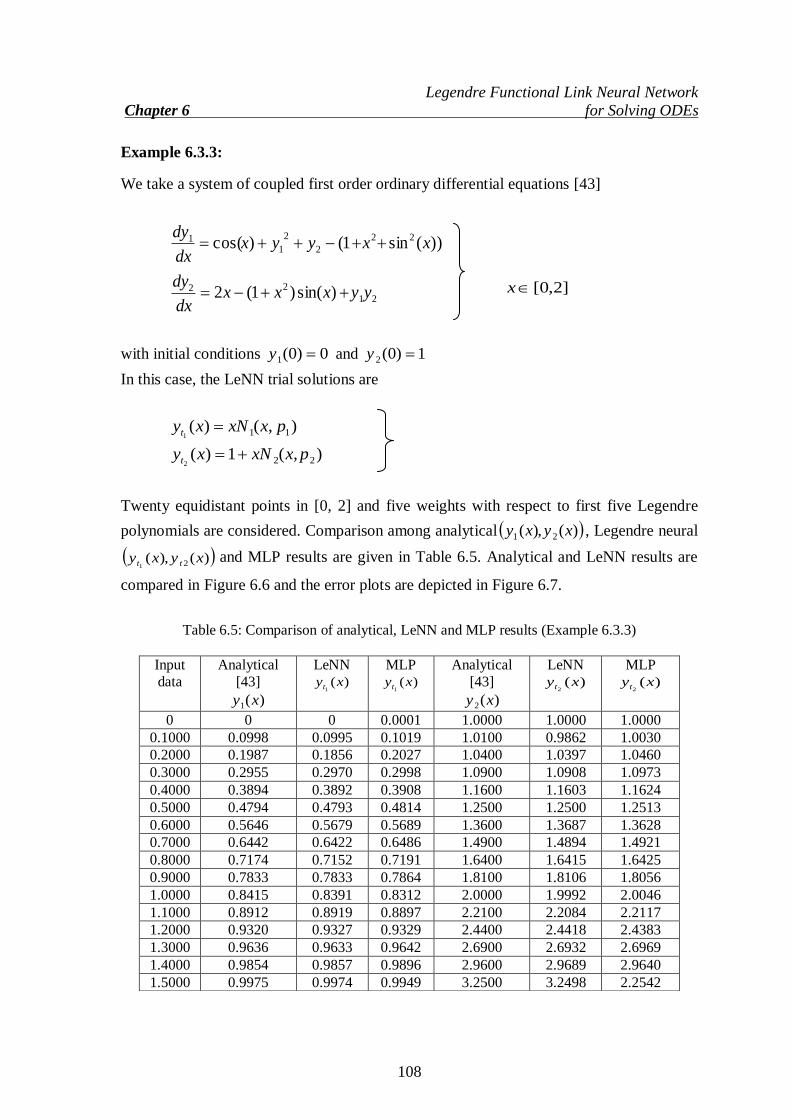
Legendre Functional Link Neural Network
Chapter 6 for Solving ODEs
108
Example 6.3.3: We take a system of coupled first order ordinary differential equations [43]
))(sin1()cos( 22
2
2
11 xxyyx
dx
dy
21
22 )sin()1(2 yyxxxdx
dy
]2,0[x
with initial conditions 0)0(1 y and 1)0(2 y
In this case, the LeNN trial solutions are
),(1)(
),()(
22
11
2
1
pxxNxy
pxxNxy
t
t
Twenty equidistant points in [0, 2] and five weights with respect to first five Legendre
polynomials are considered. Comparison among analytical )(),( 21 xyxy , Legendre neural
)(),( 21xyxy tt
and MLP results are given in Table 6.5. Analytical and LeNN results are
compared in Figure 6.6 and the error plots are depicted in Figure 6.7.
Table 6.5: Comparison of analytical, LeNN and MLP results (Example 6.3.3)
Input
data
Analytical
[43] )(1 xy
LeNN )(
1xyt
MLP
)(1
xyt
Analytical
[43]
)(2 xy
LeNN )(
2xyt
MLP
)(2
xyt
0 0 0 0.0001 1.0000 1.0000 1.0000
0.1000 0.0998 0.0995 0.1019 1.0100 0.9862 1.0030
0.2000 0.1987 0.1856 0.2027 1.0400 1.0397 1.0460
0.3000 0.2955 0.2970 0.2998 1.0900 1.0908 1.0973
0.4000 0.3894 0.3892 0.3908 1.1600 1.1603 1.1624
0.5000 0.4794 0.4793 0.4814 1.2500 1.2500 1.2513
0.6000 0.5646 0.5679 0.5689 1.3600 1.3687 1.3628
0.7000 0.6442 0.6422 0.6486 1.4900 1.4894 1.4921
0.8000 0.7174 0.7152 0.7191 1.6400 1.6415 1.6425
0.9000 0.7833 0.7833 0.7864 1.8100 1.8106 1.8056
1.0000 0.8415 0.8391 0.8312 2.0000 1.9992 2.0046
1.1000 0.8912 0.8919 0.8897 2.2100 2.2084 2.2117
1.2000 0.9320 0.9327 0.9329 2.4400 2.4418 2.4383
1.3000 0.9636 0.9633 0.9642 2.6900 2.6932 2.6969
1.4000 0.9854 0.9857 0.9896 2.9600 2.9689 2.9640
1.5000 0.9975 0.9974 0.9949 3.2500 3.2498 2.2542

Legendre Functional Link Neural Network
Chapter 6 for Solving ODEs
109
Figure 6.6: Plot of analytical and LeNN results (Example 6.3.3)
Figure 6.7: Error plots between analytical and LeNN results (Example 6.3.3)
0 0.2 0.4 0.6 0.8 1 1.2 1.4 1.6 1.8 20
0.5
1
1.5
2
2.5
3
3.5
4
4.5
5
x
Resu
lts
Analytical y1
LeNN yt1
Analytical y2
LeNN yt2
0 0.2 0.4 0.6 0.8 1 1.2 1.4 1.6 1.8 2-0.015
-0.01
-0.005
0
0.005
0.01
0.015
x
Erro
r
Accuracy of the first LeNN yt1
results
0 0.2 0.4 0.6 0.8 1 1.2 1.4 1.6 1.8 2-0.03
-0.02
-0.01
0
0.01
0.02
0.03
x
Erro
r
Accuracy of the second LeNN yt2
results
1.6000 0.9996 0.9962 0.9960 3.5600 3.5705 3.5679
1.7000 0.9917 0.9911 0.9907 3.8900 3.8911 3.8970
1.8000 0.9738 0.9800 0.9810 4.2400 4.2402 4.2468
1.9000 0.9463 0.9464 0.9470 4.6100 4.6129 4.6209
2.0000 0.9093 0.9096 0.9110 5.0000 4.9995 5.0012

Legendre Functional Link Neural Network
Chapter 6 for Solving ODEs
110
Example 6.3.4: In this Example, system of coupled first order ordinary differential equations is taken
)sin(
)sin()cos(
212
2
1
xeyydx
dy
y
xx
dx
dy
x
]2,0[x
subject to 0)0(1 y and 1)0(2 y
Analytical solutions for the above may be obtained as
x
x
exy
e
xxy
)(
)sin()(
2
1
Corresponding LeNN trial solutions are
),(1)(
),()(
22
11
2
1
pxxNxy
pxxNxy
t
t
The network is trained here for twenty equidistant points in the given domain. As in
previous cases, the analytical, LeNN and MLP results are shown in Table 6.6.
Comparisons between analytical )(),( 21 xyxy and LeNN )(),( 21xyxy tt
results are
depicted in Figure 6.8 and are found to be in excellent agreement. Plot of the error
function is cited in Figure 6.9. Lastly, LeNN solutions for some testing points are given in
Table 6.7.
Table 6.6: Comparison of analytical, LeNN and MLP results (Example 6.3.4)
Input data Analytical
)(1 xy
LeNN )(
1xyt
MLP
)(1
xyt
Analytical
)(2 xy
LeNN )(
2xyt
MLP
)(2
xyt
0 0 0 0 1.0000 1.0000 1.0000
0.1000 0.0903 0.0907 0.0899 1.1052 1.1063 1.1045
0.2000 0.1627 0.1624 0.1667 1.2214 1.2219 1.2209
0.3000 0.2189 0.2199 0.2163 1.3499 1.3505 1.3482
0.4000 0.2610 0.2609 0.2625 1.4918 1.5002 1.4999
0.5000 0.2908 0.2893 0.2900 1.6487 1.6477 1.6454
0.6000 0.3099 0.3088 0.3111 1.8221 1.8224 1.8209

Legendre Functional Link Neural Network
Chapter 6 for Solving ODEs
111
Table 6.7: Analytical, LeNN results for testing points (Example 6.3.4)
Figure 6.8: Plot of analytical and LeNN results (Example 6.3.4)
0 0.2 0.4 0.6 0.8 1 1.2 1.4 1.6 1.8 20
1
2
3
4
5
6
7
8
x
Resu
lts
Analytical y1
LeNN yt1
Analytical y2
LeNN yt2
0.7000 0.3199 0.3197 0.3205 2.0138 2.0158 2.0183
0.8000 0.3223 0.3225 0.3234 2.2255 2.2246 2.2217
0.9000 0.3185 0.3185 0.3165 2.4596 2.4594 2.4610
1.0000 0.3096 0.3093 0.3077 2.7183 2.7149 2.7205
1.1000 0.2967 0.2960 0.2969 3.0042 3.0043 3.0031
1.2000 0.2807 0.2802 0.2816 3.3201 3.3197 3.3211
1.3000 0.2626 0.2632 0.2644 3.6693 3.6693 3.6704
1.4000 0.2430 0.2431 0.2458 4.0552 4.0549 4.0535
1.5000 0.2226 0.2229 0.2213 4.4817 4.4819 4.4822
1.6000 0.2018 0.2017 0.2022 4.9530 4.9561 4.9557
1.7000 0.1812 0.1818 0.1789 5.4739 5.4740 5.4781
1.8000 0.1610 0.1619 0.1605 6.0496 6.0500 6.0510
1.9000 0.1415 0.1416 0.1421 6.6859 6.6900 6.6823
2.0000 0.1231 0.1230 0.1226 7.3891 7.3889 7.3857
Testing points 0.3894 0.7120 0.9030 1.2682 1.5870 1.8971
Analytical y1 0.2572 0.3206 0.3183 0.2686 0.2045 0.1421
LeNN yt1 0.2569 0.3210 0.3180 0.2689 0.2045 0.1420
Analytical y2 1.4761 2.0381 2.4670 3.5544 4.8891 6.6665
LeNN yt2 1.4760 2.0401 2.4672 3.5542 4.8894 6.6661

Legendre Functional Link Neural Network
Chapter 6 for Solving ODEs
112
Figure 6.9: Error plots between analytical and LeNN results (Example 6.3.4)
The CPU time of computation for the proposed LeNN model and traditional neural
network (MLP) are incorporated in Table 6.8. As such we may see that LeNN takes less
time of computation than traditional MLP.
Table 6.8: CPU time of computation
CPU time of
computation (in Sec.)
Example
6.3.1
Example
6.3. 2
Example
6.3.3
Example
6.3.4
MLP 11,849.45 8,108,71 11,987.25 12,368.15
LeNN 9,170.89 7,212,38 10,723.09 10,288.26
Next, we have compared different ANN techniques viz. traditional MLP, single layer
ChNN and LeNN for solving Lane-Emden and Emden-Fowler equations. Homogeneous
Lane-Emden and Emden-Fowler equation are discussed in Examples 6.3.5 and 6.3.6
respectively.
Example 6.3.5: Let us consider second order homogeneous Lane-Emden equation
0)32(22 2
2
2
yxdx
dy
xdx
yd
10 x
with initial conditions 1)0( y , 0)0( y
0 0.2 0.4 0.6 0.8 1 1.2 1.4 1.6 1.8 2-0.01
-0.008
-0.006
-0.004
-0.002
0
0.002
0.004
0.006
0.008
0.01
x
Erro
r
Accuracy of the first LeNN yt1
results
0 0.2 0.4 0.6 0.8 1 1.2 1.4 1.6 1.8 2-0.01
-0.008
-0.006
-0.004
-0.002
0
0.002
0.004
0.006
0.008
0.01
xE
rro
r
Accuracy of the second LeNN yt2
results

Legendre Functional Link Neural Network
Chapter 6 for Solving ODEs
113
The analytical solution of the above equation is given in [84] as
2
)( xexy
As mentioned in Sec. 2.2.2 (Eq. 2.18), we have the trial solution as
),(1),( 2 pxNxpxyt
The network is trained for ten equidistant points in the given domain [0, 1]. We have
considered six hidden nodes for MLP and six polynomials (Chebyshev, Legendre) for
single layer neural network. Table 6.9 shows comparison among analytical [84]
traditional MLP, ChebyshevNeural Network (ChNN) and Legendre Neural Network
(LeNN) solutions. Also, comparison among analytical, traditional MLP, ChNN and LeNN
results are also depicted in Figure 6.10.
Table 6.9: Comparison among analytical, MLP, ChNN and LeNN solutions (Example 6.3.5)
Figure 6.10: Plot of analytical, MLP, ChNN and LeNN solutions (Example 6.3.5)
0 0.1 0.2 0.3 0.4 0.5 0.6 0.7 0.8 0.9 10.8
1
1.2
1.4
1.6
1.8
2
2.2
2.4
2.6
2.8
x
Res
ult
s
Analytical
MLP
ChNN
LeNN
Input data Analytical [84] MLP ChNN LeNN
0 1.0000 1.0008 1.0001 0.9999
0.1 1.0101 1.0201 1.0094 1.0178
0.2 1.0408 1.0614 1.0421 1.0442
0.3 1.0942 1.1257 1.0945 1.0936
0.4 1.1732 1.1363 1.1598 1.1879
0.5 1.2840 1.2747 1.2866 1.2856
0.6 1.4333 1.5468 1.4312 1.4481
0.7 1.6323 1.6197 1.6238 1.6380
0.8 1.8965 1.9176 1.8924 1.8645
0.9 2.2479 2.2242 2.2392 2.2435
1.0 2.7148 2. 7320 2.7148 2.7201

Legendre Functional Link Neural Network
Chapter 6 for Solving ODEs
114
In view of the above one may see that the analytical results compared very well with
ChNN and LeNN results.
Example 6.3.6: In this example we take a non linear Emden- Fowler equation.
yyyyx
y ln4146
0x
subject to 1)0( y , 0)0( y
We can write the trial solution as
),(1),( 2 pxNxpxyt
Here we have trained the network for ten equidistant points in [0, 1]. Comparison among
analytical [80], traditional MLP, single layer ChNN and LeNN results are given in Table
6.10. Analytical, MLP, ChNN and LeNN results are compared in Figure 6.11.
Table 6.10: Comparison among analytical, MLP, ChNN and LeNN solutions (Example 6.3.6)
The CPU time of computation for Examples 6.3.5 and 6.3.6 are incorporated in Table
6.11. It may be seen that ChNN and LeNN require less time than MLP. Moreover,
between ChNN and LeNN, the ChNN requires less CPU time of computation for the
present problems (Examples 6.3.5 and 6.3.6).
Input data Analytical
[80]
MLP
ChNN LeNN
0 1.0000 1.0000 1.0002 1.0002
0.1 0.9900 0.9914 0.9901 0.9907
0.2 0.9608 0.9542 0.9606 0.9602
0.3 0.9139 0.9196 0.9132 0.9140
0.4 0.8521 0.8645 0.8523 0.8503
0.5 0.7788 0.7710 0.7783 0.7754
0.6 0.6977 0.6955 0.6974 0.6775
0.7 0.6126 0.6064 0.6116 0.6125
0.8 0.5273 0.5222 0.5250 0.5304
0.9 0.4449 0.4471 0.4439 0.4490
1.0 0.3679 0.3704 0.3649 0.3696

Legendre Functional Link Neural Network
Chapter 6 for Solving ODEs
115
Figure 6.11: Plot of analytical, MLP, ChNN and LeNN solutions (Example 6.3.6)
Table 6.11: CPU time of computation
CPU time of computation
(in Sec.)
MLP ChNN LeNN
Example 6.3.5 10,168.41 8,552.15 8,869.19
Example 6.3.6 9,588.26 7,716.49 8,142.33
6.4 Conclusion
In this chapter, we have proposed a single layer Legendre Neural Network (LeNN) model
to solve ordinary differential equations viz. nonlinear singular initial value problem of
Lane-Emden type, second order boundary value problem and system of coupled first
order ODEs. Here we have considered single layer Functional Link Artificial Neural
Network (FLANN) architecture. The dimension of input data is expanded using the set of
Legendre orthogonal polynomials. Excellent agreement of the results between analytical
and LeNN show the powerfulness and reliability of the proposed method.
0 0.1 0.2 0.3 0.4 0.5 0.6 0.7 0.8 0.9 1
0.4
0.5
0.6
0.7
0.8
0.9
1
1.1
x
Resu
lts
Analytical
MLP
ChNN
LeNN

116
Chapter 7
Simple Orthogonal Polynomial Based
Functional Link Neural Network Model
for Solving ODEs
Single layer Simple Orthogonal Polynomial based Functional Link Artificial Neural
Network (FLANN) model has been proposed in this chapter. We have considered Gram-
Schmidt orthogonal polynomial based FLANN model to obtain the numerical solution of
force-free Duffing equations with various initial conditions for the first time. The present
method eliminates the hidden layer by expanding the input patterns using Gram-Schmidt
orthogonal polynomials. Feed forward neural model for single input, single output and
back propagation algorithm have been used here. Results obtained by Simple Orthogonal
Polynomial based Neural Network (SOPNN) are compared with the results obtained by
other numerical methods. Accuracy of SOPNN, errors and phase diagrams are also shown
graphically.*
7.1 Simple Orthogonal Polynomial based Neural Network
(SOPNN) Model
In this head, we have described the architecture of single layer SOPNN model, SOPNN
formulation for ODEs, learning algorithm and computation of gradient.
*Content of this chapter has been communicated in the following Journal:
1. Applied Mathematical Modeling, (under review), (2014).

Simple Orthogonal Polynomial Based
Chapter 7 FLNN Model for Solving ODEs
117
7.1.1 Architecture of Simple Orthogonal Polynomial based Neural
Network (SOPNN) Model
A single layer Simple Orthogonal polynomial based Neural Network model has been
considered here. Figure 7.1 gives the structure of Simple Orthogonal Polynomial based
Neural Network (SOPNN) which consists of single input node, single output node and a
functional expansion block based on Gram-Schmidt orthogonal polynomials. The SOPNN
model consists of two parts, the first one is numerical transformation part and the second
part is learning part. In numerical transformation part, each input data of SOPNN model is
expanded to several terms using Gram-Schmidt orthogonal polynomials. We have
considered only one input node. For the linearly independent sequence ,...},,,1{ 32 uuu
first six orthogonal polynomials obtained by Gram-Schmidt process are well known and
may be written as
252
1
42
5
6
5
9
20
2
5)(
70
1
7
2
7
92)(
20
1
5
3
2
93)(
6
1)(
2
1)(
1)(
2345
5
234
4
23
3
2
2
1
0
uuuuuu
uuuuu
uuuu
uuu
uu
u
(7.1)
We have considered input data (time) as T
htttt ),...,,( 21 that is the single node t has h
number of data.

Simple Orthogonal Polynomial Based
Chapter 7 FLNN Model for Solving ODEs
118
)(0 t 1v
)(1 t 2v
)(4 t
Figure 7.1: Architecture of single layer SOPNN
7.1.2 Formulation and Learning Algorithm of Proposed SOPNN Model
General formulation for ODEs using ANN has been discussed in Sec. 2.2.1.
The SOPNN trial solution ),( ptx for ODEs with input t and parameters p may be
expressed as
)),(,()(),( ptNtFtAptx (7.2)
The first term )(tA satisfies only initial/boundary conditions, where as the second term
)),(,( ptNtF contains the single output ),( ptN of SOPNN with input t and adjustable
parameters (weights) p. The tangent hyperbolic function is considered here as the
activation function.
As mentioned above, a single layer SOPNN is considered with one input node and
single output node ),( ptN is formulated as
zz
zz
ee
eezptN
)tanh(),( (7.3)
where z a linear combination of expanded input data. It is written as
t
),( ptN
Input layer SOPNN Output
Output layer
)tanh(
)(3 t
)(5 t
4v
5v
6v
)(2 t
3v
Sim
ple
Ort
hogon
al
E
xp
an
sion

Simple Orthogonal Polynomial Based
Chapter 7 FLNN Model for Solving ODEs
119
)(1
1
tvz j
m
j
j
(7.4)
where t (time) is the input data, )(1 tj and jv with },...3,2,1{ mj denote the expanded
input data and weight vector respectively of the SOPNN model.
Let us consider now the formulation for the second order ordinary differential
equation in particular because our aim is here to solve the Duffing and Van der Pol-
Duffing oscillator equations.
The targeted differential equation may be written as
),,(2
2
dt
dxxtf
dt
xd
bat ,
(7.5)
with initial conditions Aax )( , Aax )(
In this regard, SOPNN formulation for second initial value problems may be written as
),()()(),( 2 ptNatatAAptx (7.6)
The error function is written as
2
2
2
1
),(),,(,
),(
2
1),(
dt
ptdxptxtf
dt
ptxdptE
i
ii
i
h
i
(7.7)
Error back propagation learning principle (unsupervised) has been used for minimizing
error function and to update the network parameters (weights) of the SOPNN model. The
weights from input to output layer are updated by taking negative gradient at each
iteration
k
j
kk
j
k
j
k
j
k
jv
ptEvvvv
),(1 (7.8)
7.1.3 Gradient Computation for SOPNN
The error computation not only involves the output but also the derivative of the network
output with respect to its input. So it requires finding out the gradient of the network
derivatives with respect to its input.
As such, the derivatives of ptN ,( ) with respect to input t is written as

Simple Orthogonal Polynomial Based
Chapter 7 FLNN Model for Solving ODEs
120
)()(
)()(1
1
2))(())((
2))(())((2))(())((
11
1111
tvee
eeee
dt
dNjj
m
j
tvtv
tvtvtvtv
jjjj
jjjjjjjj
(7.9)
Similarly, we can find other derivatives as (in Sec. 2.2.5, Eq. 2.44 and Eq. 2.49). Using
unsupervised training as given in Sec. 2.2.2 (Eq. 2.9) we may minimize the error function
as per the desired accuracy.
7.2 Duffing Oscillator Equations
Duffing oscillators play a crucial role in applied mathematics, physics and engineering
problems. The nonlinear Duffing oscillator equations have various engineering
applications viz. nonlinear vibration of beams and plates [93], magneto-elastic mechanical
systems [94] and fluid flow induced vibration [95] etc.
A solution of the above problems has been a recent research topic because most of
them do not have analytical solutions. So various numerical techniques and perturbation
methods have been used to handle Duffing oscillator equations [96--101] etc. But our aim
is to solve these equations using single layer SOPNN method.
Governing equation The general form of damped Duffing oscillator equation is expressed as
tFxxdt
dx
dt
xd cos3
2
2
0 (7.10)
with initial conditions ax )0( , bx )0(
Here represents the damping coefficient, F and denote the magnitude of periodic
force and frequency of the force respectively and t is the periodic time.
Eq. (7.10) reduces to unforced damped Duffing oscillator equation when F=0.
The unforced Van der Pol Duffing oscillator equation may be written as
0)( 3
2
2
xxdt
dxx
dt
xd (7.11)
subject to ax )0( , bx )0(
where ,, and are arbitrary constants.

Simple Orthogonal Polynomial Based
Chapter 7 FLNN Model for Solving ODEs
121
7.3 Case Studies
This section includes unforced damped Duffing oscillator and Van der Pol-Duffing
oscillator equations to show the powerfulness of the proposed method. We have taken
unforced Duffing oscillator equations in Examples 7.3.1 and 7.3.2 respectively. Then an
unforced Van der Pol-Duffing oscillator is given in Example 7.3.3.
Example 7.3.1: Let us take a force-free damped Duffing oscillator problem [97]
with ,5.0 ,25 1.0a and .0b
Accordingly we have
025255.0 3
2
2
xxdt
dx
dt
xd
subject to initial conditions 1.0)0( x , .0)0( x
As discussed above we may write the SOPNN trial solution as
),(1.0),( 2 ptNtptx The network has been trained for 50 points in the domain [0, 5] with six weights with
respect to first six simple orthogonal polynomials. Table 7.1 shows comparison among
numerical solutions obtained by Modified Differential Transformation Method (MDTM)
[97] by the Pade approximate of [3/3], real part of MDTM by the Pade approximate of
[4/4] and SOPNN. Comparison between results by real part of MDTM [97] and present
SOPNN are depicted in Figure 7. 2. The plot of the error function (MDTM and SOPNN)
has also been shown in Figure 7.3. The phase plane diagram is cited in Figure 7.4.
Table 7.1: Comparison between MDTM and SOPNN results (Example 7.3.1)
Input data
t (Time)
MDTM by the Pade approximate of [3/3]
[97]
real part of MDTM by the Pade
approximate of
[4/4] [97]
SOPNN
0 0.0998 0.1000 0.1000
0.1000 0.0876 0.0853 0.0842
0.2000 0.0550 0.0511 0.0512
0.3000 0.0110 0.0064 0.0063
0.4000 -0.0331 -0.0380 -0.0377
0.5000 -0.0665 -0.0712 -0.0691
0.6000 -0.0814 -0.0854 -0.0856
0.7000 -0.0751 -0.0782 -0.0764

Simple Orthogonal Polynomial Based
Chapter 7 FLNN Model for Solving ODEs
122
0.8000 -0.0502 -0.0528 -0.0530
0.9000 -0.0136 -0.0161 -0.0173
1.0000 0.0249 0.0229 0.0224
1.1000 0.0560 0.0547 0.0539
1.2000 0.0722 0.0716 0.0713
1.3000 0.0704 0.0703 0.0704
1.4000 0.0518 0.0523 0.0519
1.5000 0.0219 0.0227 0.0215
1.6000 -0.0115 -0.0110 -0.0109
1.7000 -0.0399 -0.0406 -0.0394
1.8000 -0.0567 -0.0589 -0.0574
1.9000 -0.0582 -0.0620 -0.0624
2.0000 -0.0449 -0.0501 -0.0489
2.1000 -0.0207 -0.0268 -0.0262
2.2000 0.0078 0.0018 -0.0018
2.3000 0.0336 0.0287 0.0279
2.4000 0.0503 0.0473 0.0477
2.5000 0.0543 0.0536 0.0534
2.6000 0.0452 0.0467 0.0461
2.7000 0.0260 0.0290 0.0289
2.8000 0.0017 0.0051 0.0052
2.9000 -0.0212 -0.0189 -0.0191
3.0000 -0.0374 -0.0372 -0.0375
3.1000 -0.0431 -0.0456 -0.0487
3.2000 -0.0375 -0.0426 -0.0404
3.3000 -0.0224 -0.0295 -0.0310
3.4000 -0.0021 -0.0101 -0.0135
3.5000 0.0182 0.0109 0.0147
3.6000 0.0335 0.0283 0.0308
3.7000 0.0404 0.0380 0.0400
3.8000 0.0374 0.0380 0.0388
3.9000 0.0259 0.0290 0.0279
4.0000 0.0090 0.0134 0.0113
4.1000 -0.0088 -0.0047 -0.0076
4.2000 -0.0230 -0.0208 -0.0221
4.3000 -0.0305 -0.0311 -0.0309
4.4000 -0.0296 -0.0334 -0.0325
4.5000 -0.0210 -0.0275 -0.0258
4.6000 -0.0072 -0.0154 -0.0124
4.7000 0.0082 -0.0001 0.0032
4.8000 0.0213 0.0145 0.0193
4.9000 0.0290 0.0248 0.0250
5.0000 0.0297 0.0287 0.0288

Simple Orthogonal Polynomial Based
Chapter 7 FLNN Model for Solving ODEs
123
Figure 7.2: Plot of MDTM and SOPNN results (Example 7.3.1)
Figure 7.3: Error plot between MDTM and SOPNN results (Example 7.3.1)
0 0.5 1 1.5 2 2.5 3 3.5 4 4.5 5-0.1
-0.08
-0.06
-0.04
-0.02
0
0.02
0.04
0.06
0.08
0.1
t
Resu
lts
MDTM by Pade 4/4
SOPNN
0 0.5 1 1.5 2 2.5 3 3.5 4 4.5 5-0.02
-0.015
-0.01
-0.005
0
0.005
0.01
0.015
0.02
t
Err
or

Simple Orthogonal Polynomial Based
Chapter 7 FLNN Model for Solving ODEs
124
Figure 7.4: Phase plane plot by SOPNN (Example 7.3.1)
Example 7.3.2: Next, we have taken the damped Duffing oscillator problem with ,1 ,20 ,2 2.0a and .2b
The differential equation may be written as
0220 3
2
2
xxdt
dx
dt
xd
subject to 2.0)0( x , .2)0( x
The SOPNN trial solution, in this case, is represented as
),(22.0),( 2 ptNttptx
Again the network is trained with 50 equidistant points in the interval [0, 5] with first six
simple orthogonal polynomials. Table 7.2 incorporates the comparison between solutions
of the real part of Modified Differential Transformation Method (MDTM) [97] by the
Pade approximate of [4/4] and SOPNN. Figure 7.5 shows comparison of results between
[97] and SOPNN. The plot of the error is cited in Figure 7.6. Again Figure 7.7 depicts the
phase plane diagram.
-0.1 -0.05 0 0.05 0.1 0.15-0.5
-0.4
-0.3
-0.2
-0.1
0
0.1
0.2
0.3
0.4
x(t)
x'(t
)
SOPNN

Simple Orthogonal Polynomial Based
Chapter 7 FLNN Model for Solving ODEs
125
Figure 7.5: Plot of MDTM and SOPNN results (Example 7.3.2)
Table 7.2: Comparison between MDTM and SOPNN results (Example 7.3.2)
0 0.5 1 1.5 2 2.5 3 3.5 4 4.5 5-0.3
-0.2
-0.1
0
0.1
0.2
0.3
0.4
t
Resu
lts
Real part of MDTM by Pade [4/4]
SOPNN
Input data t (Time)
MDTM [97]
SOPNN
0 -0.2000 -0.2000
0.1000 0.0031 0.0034
0.2000 0.1863 0.1890
0.3000 0.3170 0.3172
0.4000 0.3753 0.3745
0.5000 0.3565 0.3587
0.6000 0.2714 0.2711
0.7000 0.1427 0.1400
0.8000 -0.0010 -0.0014
0.9000 -0.1307 -0.1299
1.0000 -0.2234 -0.2250
1.1000 -0.2648 -0.2639
1.2000 -0.2519 -0.2510
1.3000 -0.1923 -0.1930

Simple Orthogonal Polynomial Based
Chapter 7 FLNN Model for Solving ODEs
126
1.4000 -0.1016 -0.1013
1.5000 -0.0002 -0.0005
1.6000 0.0916 0.0919
1.7000 0.1574 0.1570
1.8000 0.1869 0.1872
1.9000 0.1781 0.1800
2.0000 0.1362 0.1360
2.1000 0.0724 0.0726
2.2000 0.0007 0.0006
2.3000 -0.0642 -0.0661
2.4000 -0.1108 -0.1095
2.5000 -0.1319 -0.1309
2.6000 -0.1259 -0.1262
2.7000 -0.0965 -0.0969
2.8000 -0.0515 -0.0519
2.9000 -0.0009 -0.0003
3.0000 0.0450 0.0456
3.1000 0.0781 0.0791
3.2000 0.0931 0.0978
3.3000 0.0890 0.0894
3.4000 0.0684 0.0671
3.5000 0.0367 0.0382
3.6000 0.0010 0.0021
3.7000 -0.0315 -0.0338
3.8000 -0.0550 -0.0579
3.9000 -0.0657 -0.0666
4.0000 -0.0629 -0.0610
4.1000 -0.0484 -0.0501
4.2000 -0.0261 -0.0285
4.3000 -0.0009 -0.0005
4.4000 0.0221 0.0210
4.5000 0.0387 0.0400
4.6000 0.0464 0.0472
4.7000 0.0445 0.0439
4.8000 0.0343 0.0358
4.9000 0.0186 0.0190
5.0000 0.0008 0.0006

Simple Orthogonal Polynomial Based
Chapter 7 FLNN Model for Solving ODEs
127
Figure 7.6: Error plot between MDTM and SOPNN results (Example 7.3.2)
Figure 7.7: Phase plane plot by SOPNN (Example 7.3.2)
Example 7.3.3: In this example an unforcedVan Der Pol-Duffing oscillator equation has been considered
as [98]
with 1,3
1,3,
3
4 and F=0
0 0.5 1 1.5 2 2.5 3 3.5 4 4.5 5-0.02
-0.015
-0.01
-0.005
0
0.005
0.01
0.015
0.02
t
Erro
r
-0.4 -0.3 -0.2 -0.1 0 0.1 0.2 0.3 0.4 0.5-2
-1.5
-1
-0.5
0
0.5
1
1.5
2
2.5
x(t)
x'(
t)
SOPNN

Simple Orthogonal Polynomial Based
Chapter 7 FLNN Model for Solving ODEs
128
Here the differential equation is
03
1)3
3
4( 3
2
2
xxdt
dxx
dt
xd
with initial conditions 2887.0)0( x , .12.0)0( x
The related SOPNN trial solution is
),(12.02887.0),( 2 ptNttptx
In this case, we have considered twenty five points in the interval [0, 10] with first six
simple orthogonal polynomials. We have compared SOPNN results with New Homotopy
Perturbation Method (NHPM) results [98] in Table 7.3. NHPM and SOPNN results are
also compared graphically in Figure 7.8. Finally, Figure 7.9 depicts the plot of error
between NHPM and SOPNN results.
Figure 7.8: Plot of MHPM [98] and SOPNN results (Example 7.3.3)
0 1 2 3 4 5 6 7 8 9 10-0.35
-0.3
-0.25
-0.2
-0.15
-0.1
-0.05
0
t
Res
ult
s
NHPM
SOPNN

Simple Orthogonal Polynomial Based
Chapter 7 FLNN Model for Solving ODEs
129
Table 7.3: Comparison between NHPM and SOPNN results (Example 7.3.3)
Input data
t (Time)
NHPM
[98]
SOPNN
0 -0.2887 -0.2887 0.4000 -0.2456 -0.2450
0.8000 -0.2106 -0.2099
1.2000 -0.1816 -0.1831
1.6000 -0.1571 -0.1512
2.0000 -0.1363 -0.1400
2.4000 -0.1186 -0.1206
2.8000 -0.1033 -0.1056
3.2000 -0.0900 -0.0912
3.6000 -0.0786 -0.0745
4.0000 -0.0686 -0.0678
4.4000 -0.0599 -0.0592
4.8000 -0.0524 -0.0529
5.2000 -0.0458 -0.0436
5.6000 -0.0400 -0.0405
6.0000 -0.0350 -0.0351
6.4000 -0.0306 -0.0297
6.8000 -0.0268 -0.0262
7.2000 -0.0234 -0.0237
7.6000 -0.0205 -0.0208
8.0000 -0.0179 -0.0180
8.4000 -0.0157 -0.0160
8.8000 -0.0137 -0.0139
9.2000 -0.0120 -0.0115
9.6000 -0.0105 -0.0113
10.0000 -0.0092 -0.0094

Simple Orthogonal Polynomial Based
Chapter 7 FLNN Model for Solving ODEs
130
Figure 7.9: Error plot between MHPM and SOPNN results (Example 7.3.3)
7.4 Conclusion
A single layer Simple Orthogonal Polynomial based Neural Network (SOPNN) has been
proposed and applied to solve unforced damped Duffing oscillator and Van der Pol-
Duffing oscillator equations. The hidden layer is eliminated by functional expansion
block for enhancement of the input patterns using simple orthogonal polynomials.
Comparison of the proposed SOPNN results with other numerical results shows that the
present method is convenient and effective for solving nonlinear Duffing oscillator
problems.
0 0.5 1 1.5 2 2.5 3 3.5 4 4.5 5-0.02
-0.015
-0.01
-0.005
0
0.005
0.01
0.015
0.02
t
Err
or

131
Chapter 8
Hermite Functional Link Neural Network
Model for Solving ODEs
In this chapter, Hermite polynomial based Functional Link Artificial Neural Network
(FLANN) named Hermite Neural Network (HeNN) has been proposed for solving the
Van der Pol-Duffing oscillator equation. The Van der Pol-Duffing oscillator equation is a
classical nonlinear oscillator which is very useful mathematical model for understanding
different engineering problems. This equation is widely used to model various physical
problems viz. electrical circuit, electronics, mechanics etc. [94]. Three mathematical
example problems and two real life application problems viz. extracting the features of
early mechanical failure signal and weak signal detection problems are solved using the
proposed HeNN method. The hidden layer is replaced by expansion block of input pattern
using Hermit orthogonal polynomials. The single layer HeNN model has some
advantages such as simpler structure and lower computational complexity due to less
number of parameters than the traditional neural network model. HeNN approximate
solutions have been compared with results obtained by other numerical methods.
Computed results are depicted in term of plots to show the validation of the
methodology.*
8.1 Hermite Neural Network (HeNN) model
In this section, architecture of single layer HeNN model, its formulation, learning
algorithm and gradient computation of network output have been introduced.
*Content of this chapter has been accepted in following Journal:
1. Neural Computation (Accepted), 2016.

Hermite Functional Link Neural Network Model
Chapter 8 for Solving ODEs
132
8.1.1 Structure of Hermite Neural Network (HeNN) Model
Figure 8.1 depicts the structure of HeNN model which consists of the single input node,
the single output node and Hermite orthogonal polynomial based functional expansion
block. HeNN model is a single layer neural model where each input data is expanded to
several terms using Hermite polynomials. The first three Hemite polynomials may be
written as
1)(
)(
1)(
2
2
1
0
xxHe
xxHe
xHe
(8.1)
Higher order Hermite polynomials may then be generated by the recursive formula
)()()(1 xeHxxHexHe nnn
(8.2)
We consider input data (time) as T
htttt ),...,,( 21 that is the single node t is assumed to
have h number of data. The architecture of the network with first seven Hermite
polynomials, single input and output nodes are shown in Figure 8.1.
Figure 8.1: Architecture of single layer Hermite Neural Network
t
),( ptN
Input layer HeNN Output
Output layer
)tanh(
)(0 tHe
)(1 tHe
)(2 tHe
)(2 tHe
)(3 tHe
)(5 tHe
)(6 tHe
3w
7w
)(4 tHe
6w
5w
4w
2w
1w
Her
mit
E
xp
an
sion

Hermite Functional Link Neural Network Model
Chapter 8 for Solving ODEs
133
8.1.2 Formulation and Learning Algorithm of Proposed HeNN Model
The HeNN trial solution ),( ptxHe for the ODEs with parameters (weights) p may be
expressed as
)),(,()(),( ptNtGtAptxHe (8.3)
The first term )(tA does not contain adjustable parameters and satisfies only
initial/boundary conditions, where as the second term )),(,( ptNtG contains the single
output ),( ptN of HeNN model with input t and adjustable parameters p.
As such, network output with input t and parameters (weights) p may be computed as
zz
zz
ee
eezptN
)tanh(),( (8.4)
where z is a linear combination of expanded input data and is written as
)(1
1
tHewz j
m
j
j
(8.5)
here t (time) is the input data, )(1 tHe j and jw with },...3,2,1{ mj denote the expanded
input data and the weight vector respectively of the HeNN.
Our aim is to solve the Van der Pol-Duffing oscillator equation. As such we have
discussed the formulation of the second order initial value problem of in Eq. 7.5 and 7.6
and error function in Eq. 7.7 (Chapter 7).
Unsupervised error back propagation learning principle (in Eqs. 2.9 to 2.12) has
been used here to update the network parameters (weights) of the Hermite Neural
Network (HeNN) model and the tangent hyperbolic function tanh(.) is considered as the
activation function.
8.1.3 Gradient Computation for HeNN
The error computation involves both output and derivative of the output with respect to
the corresponding input. So it is required to find the gradient of the network derivatives
with respect to the input.
As such, the derivatives of ptN ,( ) with respect to input t is written as

Hermite Functional Link Neural Network Model
Chapter 8 for Solving ODEs
134
m
j
jjtHewtHew
tHewtHewtHewtHew
teHwee
eeee
dt
dNjjjj
jjjjjjjj
1
12))(())((
2))(())((2))(())((
)()(
)()(11
1111
(8.6)
Similarly, the second derivative of N(t,p) is computed as
m
j
jjxHewxHew
xHewxHew
jjxHewxHew
xHewxHew
xHewxHew
xHewxHew
xeHwee
ee
xeHwee
ee
ee
ee
dt
Nd
jjjj
jjjj
jjjj
jjjj
jjjj
jjjj
1
1
2
))(())((
))(())((
2
1))(())((
))(())((3
))(())((
))(())((
2
2
)(1
)(22
11
11
11
11
11
11
(8.7)
where jw denote weights and )(),( 11 xeHxeH jj denote first and second derivatives of
Hermite polynomials.
8.2 The Van der Pol-Duffing Oscillator Equation
The Van der Pol-Duffing oscillator equation is a classical nonlinear oscillator which is a
very useful mathematical model for understanding different engineering problems. This
equation is widely used to model various physical problems viz. electrical circuit,
electronics, mechanics etc. [94]. The Van der Pol oscillator equation was proposed by a
Dutch scientist Balthazar Van der Pol, which describes triode oscillations in electrical
circuits. The Van der Pol- Duffing oscillator is a classical example of the self oscillatory
system and is now considered as the very important model to describe variety of physical
systems. Also, this equation describes self-sustaining oscillations in which energy is fed
into small oscillations and removed from large oscillations. The Van der Pol-Duffing
oscillator equation has been used in various real life problems. Few of them may be
mentioned here. Hu and Wen [112] applied the Duffing oscillator for extracting the
features of early mechanical failure signal. Zhihong and Shaopu [113] used Van der Pol
Duffing oscillator equation for weak signal detection. Amplitude and phase of the weak
signal have been determined by [114] using Duffing oscillator equation. Tamaseviciute et
al. [115] investigated an extremely simple analogue electrical circuit simulating the two-
well Duffing-Holmes oscillator equation. The weak periodic signals and machinery faults
have been explained by Li and Qu [116]. The nonlinear Duffing oscillator and Van der
Pol-Duffing oscillator equations are difficult to solve analytically. In recent years, various

Hermite Functional Link Neural Network Model
Chapter 8 for Solving ODEs
135
types of numerical and perturbation techniques such as Runge-Kutta, homotopy
perturbation, linearization, variational iteration methods have been used to solve the
nonlinear equation [103--110] etc. The objective of the present chapter is to propose
Hemite Neural Network (HeNN) to solve the Van der Pol-Duffing oscillator equations.
Model Equation
The Van der Pol-Duffing oscillator equation is governed by a second order nonlinear
differential equation
tFxxdt
dxx
dt
xd cos)1( 32
2
2
(8.8)
with initial conditions ,)0( ax bx )0(
where x stands for displacement, is the damping parameter, F and denote the
excitation amplitude and frequency of the periodic force respectively and t is the periodic
time. is known as phase nonlinearity parameter.
8.3 Numerical Examples and Discussion
In this section, the Van der Pol-Duffing oscillator equation and two application problems
have been investigated to show the efficiency of the proposed method. Two Van der Pol-
Duffing oscillator equations with force are considered in Examples 8.3.1 and 8.3.2. A
Duffing oscillator equation with force is taken in Examples 8.3.3. We have discussed two
real life application problems viz. (i) a Duffing oscillator equation used for extracting the
features of early mechanical failure signal and detect the early fault in Example 8.3.4 and
(ii) the Van der Pol-Duffing oscilator equation applied for weak signal detection in
Example 8.3.5.
Example 8.3.1: First, we take the Van der Pol-Duffing oscillator equation [108] as
txxdt
dxx
dt
xdcos53.0)1(2.0 32
2
2
subject to initial conditions 1.0)0( x , 2.0)0( x
The HeNN trial solution, in this case, is represented as

Hermite Functional Link Neural Network Model
Chapter 8 for Solving ODEs
136
),(2.01.0),( 2 ptNttptxHe
The network has been trained with 250 equidistant points in the domain that is from 0t
to 50t sec. for computing the results. We have considered seven weights with respect to
first seven Hermite polynomials for the present problem. Here t denotes the periodic time
and x(t) is the displacement at time t. Comparison between numerical results obtained by
fourth-order Runge Kutta Method (RKM) and HeNN are depicted in Figure 8.2. The
phase plane diagram that is plots between )(tx (displacement) and )(tx (velocity) for
HeNN and RKM are shown in Figures 8.3 and 8.4. Then results for some testing points
are shown in Table 8.1. This testing is done to check whether the converged HeNN can
give results directly by inputting the points which were not taken during training.
Figure 8.2: Plot of RKM and HeNN results (Example 8.3.1)
0 5 10 15 20 25 30 35 40 45 50-2.5
-2
-1.5
-1
-0.5
0
0.5
1
1.5
2
2.5
Time t
Dis
plac
emen
t
x(t)
RKM
HeNN
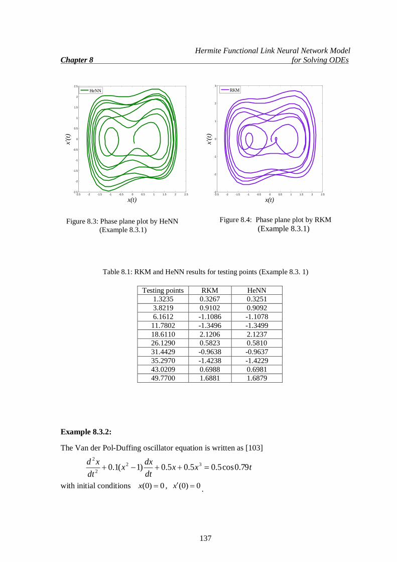
Hermite Functional Link Neural Network Model
Chapter 8 for Solving ODEs
137
Figure 8.3: Phase plane plot by HeNN
(Example 8.3.1)
Table 8.1: RKM and HeNN results for testing points (Example 8.3. 1)
Example 8.3.2: The Van der Pol-Duffing oscillator equation is written as [103]
txxdt
dxx
dt
xd79.0cos5.05.05.0)1(1.0 32
2
2
with initial conditions 0)0( x , 0)0( x .
-2.5 -2 -1.5 -1 -0.5 0 0.5 1 1.5 2 2.5-2.5
-2
-1.5
-1
-0.5
0
0.5
1
1.5
2
2.5
x(t)
x'(t
)
HeNN
-2.5 -2 -1.5 -1 -0.5 0 0.5 1 1.5 2 2.5-3
-2
-1
0
1
2
3
x(t)
x'(
t)
RKM
Testing points RKM HeNN
1.3235 0.3267 0.3251
3.8219 0.9102 0.9092
6.1612 -1.1086 -1.1078
11.7802 -1.3496 -1.3499
18.6110 2.1206 2.1237
26.1290 0.5823 0.5810
31.4429 -0.9638 -0.9637
35.2970 -1.4238 -1.4229
43.0209 0.6988 0.6981
49.7700 1.6881 1.6879
Figure 8.4: Phase plane plot by RKM
(Example 8.3.1)

Hermite Functional Link Neural Network Model
Chapter 8 for Solving ODEs
138
HeNN trial solution may be written as
),(),( 2 ptNtptxHe
In this case, 250 equidistant points from t=0 to t=50sec. and seven weights with respect
to first seven Hermite polynomials have been considered for present problem. RKM and
HeNN results are compared in Figure 8.5. Finally, Figures 8.6 and 8.7 show the phase
plane plots obtained by the methods of HeNN and RKM respectively.
Figure 8.5: Plot of RKM and HeNN results (Example 8.3.2)
0 5 10 15 20 25 30 35 40 45 50-2
-1.5
-1
-0.5
0
0.5
1
1.5
2
Time t
Dis
pla
cem
ent
x(t)
RKM
HeNN

Hermite Functional Link Neural Network Model
Chapter 8 for Solving ODEs
139
Figure 8.6: Phase plane plot by HeNN (Example 8.3.2)
Example 8.3.3: In this Example a Duffing oscillator equation with force is taken as [106]
txxdt
xd2sin2.0)2.0(3.0 322
2
2
with initial conditions 15.0)0( x , 0)0( x
As discussed in Eq. 7.6, the HeNN trial solution is constructed as
),(15.0),( 2 ptNtptxHe
Again the network is trained with 225 equidistant points in the time interval [0, 45] with
seven first Hermite polynomials. Figure 8.8 shows comparison of numerical results )(tx
among RKM, HeNN and Algebraic method (AGM) [106]. Again Figures 8.9 and 8.10
depict the phase plane diagram between displacement and velocity using HeNN and RKM
respectively. From Figure 8.8 one may see that results obtained by RKM and AGM
exactly agree at all points with HeNN results.
-2.5 -2 -1.5 -1 -0.5 0 0.5 1 1.5 2 2.5-3
-2
-1
0
1
2
3
x(t)
x'(
t)
HeNN
-2.5 -2 -1.5 -1 -0.5 0 0.5 1 1.5 2 2.5-3
-2
-1
0
1
2
3
x(t)x'(
t)
RKM
Figure 8.7: Phase plane plot by RKM
(Example 8.3.2)

Hermite Functional Link Neural Network Model
Chapter 8 for Solving ODEs
140
Figure 8.8: Plot of RKM, HeNN and AGM [106] results (Example 8.3.3)
0 5 10 15 20 25 30 35 40 45-0.5
-0.4
-0.3
-0.2
-0.1
0
0.1
0.2
0.3
0.4
0.5
Time t
Dis
pla
cem
ent
x(t
)
RKM
HeNN
AGM
-0.5 -0.4 -0.3 -0.2 -0.1 0 0.1 0.2 0.3 0.4 0.5-0.25
-0.2
-0.15
-0.1
-0.05
0
0.05
0.1
0.15
0.2
0.25
x(t)
x'(
t)
HeNN
-0.5 -0.4 -0.3 -0.2 -0.1 0 0.1 0.2 0.3 0.4 0.5-0.25
-0.2
-0.15
-0.1
-0.05
0
0.05
0.1
0.15
0.2
0.25
x(t)
x'(
t)
RKM
Figure 8.9: Phase plane plot by HeNN (Example 8.3.3)
Figure 8.10: Phase plane plot by RKM (Example 8.3.3)

Hermite Functional Link Neural Network Model
Chapter 8 for Solving ODEs
141
Example 8.3.4: A Duffing oscillator equation used for extracting the features of early mechanical failure
signal and detects the early fault has been taken [112]
)(cos3
2
2
tstxxdt
dx
td
dx
subject to 0.1)0( x , 0.1)0( x
where ,5.0 8275.0 (Amplitude of external exciting periodic force) and
tts cos0005.0)( (frequency of external weak signal). The first term of the right side of
the above equation is the reference signal and the second term is the signal to be detected.
varies from small to big the system varies from small periodic motion to chaotic motion
and at last, to great periodic motion.
For the above problem, we may write the HeNN trial solution as
),(0.10.1),( 2 ptNttptxHe
We have considered time t from 0 to 500 sec., step length h=1.0 and seven weights with
respect to first seven Hermite polynomials. The authors [112] solved the problem by
Runge Kutta method (RKM) and we used the same method to obtain their solution. The
time series plots by RKM [112] and HeNN have been shown in Figures 8.11 and 8.12.
The phase plane plots obtained by HeNN and RKM [112] method for 8275.0 have
been depicted in Figures 8.13 and 8.14. Similarly, phase plane plots for 828.0 by
HeNN and RKM [112] are given in Figures 8.15 and 8.16.
Figure 8.11: Time series diagram of RKM [112] (Example 8.3.4)
0 50 100 150 200 250 300 350 400 450 500-2
-1.5
-1
-0.5
0
0.5
1
1.5
2
Time t
Dis
plac
emen
t x
(t)
RKM

Hermite Functional Link Neural Network Model
Chapter 8 for Solving ODEs
142
Figure 8.12: Time series diagram of HeNN (Example 8.3.4)
0 50 100 150 200 250 300 350 400 450 500-2
-1.5
-1
-0.5
0
0.5
1
1.5
2
Time t
Dis
pla
cem
ent
x(t
)
HeNN
-2 -1.5 -1 -0.5 0 0.5 1 1.5 2-1.5
-1
-0.5
0
0.5
1
1.5
x(t)
x'(
t)
HeNN
-2 -1.5 -1 -0.5 0 0.5 1 1.5 2-1.5
-1
-0.5
0
0.5
1
1.5
x(t)
x'(
t)
RKM
Figure 8.13: Phase plane plot by HeNN (Example 8.3.4)
Figure 8.14: Phase plane plot by RKM [112] (Example 8.3. 4)

Hermite Functional Link Neural Network Model
Chapter 8 for Solving ODEs
143
Example 8.3.5: Finally, the Van der Pol-Duffing oscillator equation applied for weak signal detection has
been written as [113]
tFxxdt
dxx
dt
xd cos)1( 32
2
2
subject to the initial conditions 1.0)0( x , 1.0)0( x
with the parameters as 5 , 01.0 , 463.2w and 9.4F
The HeNN trial solution in this case is
),(1.01.0),( 2 ptNttptxHe
Again the network is trained for total time t=300 Sec. and h=0.5. It may be noted that
[113] have solved the problem by fourth order Runge Kutta method (RKM). The time
series plots by RKM [113] and HeNN methods are depicted in Figures 8.17 and 8.18.
Lastly, the phase plane plots by using the methods of RKM [113] and HeNN have been
given in Figures 8.19 and 8.20.
It may be noted that the amplitude of force F varies from small to large, the Van der
Pol-Duffing system varies from the chaos to the periodic state. The results show that the
orbits maintain the chaotic state. The detected signal can be viewed as a perturbation of
the main sinusoidal deriving force tF cos . The noise can only affect the local trajectory
on phase plane diagram without causing any phase transition.
-2 -1.5 -1 -0.5 0 0.5 1 1.5 2-1.5
-1
-0.5
0
0.5
1
1.5
x(t)
x'(t
)
HeNN
-2 -1.5 -1 -0.5 0 0.5 1 1.5 2-1.5
-1
-0.5
0
0.5
1
1.5
x(t)
x'(t
)
RKM
Figure 8.16: Phase plane plot by RKM [112] (Example 8.3. 4)
Figure 8.15: Phase plane plot by HeNN (Example 8.3. 4)

Hermite Functional Link Neural Network Model
Chapter 8 for Solving ODEs
144
Figure 8.17: Time series diagram of RKM [113] (Example 8.3.5)
Figure 8.18: Time series diagram of HeNN (Example 8.3.5)
0 50 100 150 200 250 300-3
-2
-1
0
1
2
3
Time t
Dis
pla
cem
en
t x
(t)
RKM
0 50 100 150 200 250 300-3
-2
-1
0
1
2
3
Time t
Dis
pla
cem
nt
x(t
)
HeNN

Hermite Functional Link Neural Network Model
Chapter 8 for Solving ODEs
145
It may be noted that the amplitude F varies from small to large, the Van der Pol Duffing
system varies from the chaos to the periodic state. Again one may see the excellent
agreement of results between RKM [113] and present (HeNN) methods for time series
results (viz. Figures 8.17 and 8.18) and phase plane plots (Figures 8.19 and 8.20).
8.4 Conclusion
Single layer Hermite Neural Network (HeNN) architecture has been considered in this
chapter to handle the Van der Pol- Duffing oscillator equation. The dimension of input
data is expanded using set of Hermite orthogonal polynomials. Thus, the numbers of
network parameters of HeNN are less than the traditional ANN model. Obtained results
have been compared with numerical results by the other methods. Excellent agreement of
the results between HeNN and other numerical methods shows the effectiveness and
reliability of the proposed method.
-2.5 -2 -1.5 -1 -0.5 0 0.5 1 1.5 2 2.5-10
-8
-6
-4
-2
0
2
4
6
8
10
x(t)
x'(
t)
RKM
-2.5 -2 -1.5 -1 -0.5 0 0.5 1 1.5 2 2.5-10
-8
-6
-4
-2
0
2
4
6
8
10
x'(
t)
x(t)
HeNN
Figure 8.19: Phase plane plot by RKM [113]
(Example 8.3.5)
Figure 8.20: Phase plane plot by HeNN
(Example 8.3.5)

146
Chapter 9
Chebyshev Functional Link Neural
Network Model for Solving
Partial Differential Equations (PDEs)
In this chapter, we mainly focus on the development of a single layer Functional Link
Artificial Neural Network (FLANN) model for solving partial differential equations
(PDEs). Numerical solution of elliptic PDEs has been obtained here by applying
Chebyshev Neural Network (ChNN) model for the first time. Computations become
efficient because the hidden layer is eliminated by expanding the input pattern by
Chebyshev polynomials. The results obtained by this method are compared with the
analytical results and are found to be in good agreement.*
9.1 Chebyshev Neural Network (ChNN) Model for PDEs
In this section, the architecture of single layer ChNN model, its learning algorithm, ChNN
of formulation for PDEs and computation of gradient have been described.
9.1.1 Architecture of Chebyshev Neural Network
A single layer Chebyshev Neural Network (ChNN) model for PDEs has been considered
for the present problem.
*Content of this chapter has been communicated in following Journal:
1. Neural Processing Letters, (under review), (2015).

Chebyshev Functional Link Neural Network Model for Solving
Chapter 9 Partial Differential Equations (PDEs)
147
Figure 9.1 shows the structure of ChNN consisting of an input layer with two input nodes
(because of two independent variables), a functional expansion block based on Chebyshev
polynomials and a single output node. The ChNN model consists of two parts, the first
one is numerical transformation part and the second part is learning algorithm of ChNN.
In numerical transformation part, each input data is expanded to several terms using
Chebyshev polynomials. Thus, the Chebyshev polynomials can be viewed as new input
vectors. The Chebyshev polynomials are a set of orthogonal polynomials obtained by a
solution of the Chebyshev differential equation. First, two Chebyshev polynomials are
known as
uuT
uT
)(
1)(
1
0 (9.1)
The higher order Chebyshev polynomials may be generated by the well known recursive
formula
)()(2)( 11 uTuuTuT nnn (9.2)
where )(xT n denotes nth order Chebyshev polynomial and -1<u<1 is the argument of the
polynomials. Here n dimensional input pattern is expanded to m dimensional enhanced
Chebyshev polynomials. We consider input pattern as 2
21 ),( RxxX T and the nodes
1x and 2x have h number of data. Then the enhanced pattern is obtained by using
Chebyshev polynomials as
),...](),(),(),...;(),(),([ 222120121110 kkkkkkxTxTxTxTxTxT
, hk ,...,2,1 (9.3)
The architecture of the network with first four Chebyshev polynomials, single input layer
(having two nodes) and an output layer (having single node) are shown in Figure 9.1.
9.1.2 Learning Algorithm of Proposed Chebyshev Neural Network
(ChNN) for PDEs
In this head, learning algorithm and procedure of applying ChNN in the solution of PDE
are discussed.

Chebyshev Functional Link Neural Network Model for Solving
Chapter 9 Partial Differential Equations (PDEs)
148
)( 10 xT
)( 11 xT
21w
31w
)( 13 xT 41w
12w
)( 20 xT 22w
)( 21 xT 32w
)( 22 xT 42w
Input layer
)( 23 xT
Figure 9.1: Structure of single layer Chebyshev Neural Network for PDEs
Unsupervised error back propagation algorithm is used for learning and the weights are
updated by taking negative gradient at each iteration. As such, the gradient of an error
function with respect to the network parameters (weights) is determined. The nonlinear
tangent hyperbolic function viz. is considered as the activation function. Weights
are initialized randomly.
9.1.3 ChNN Formulation for PDEs
We write the trial solution for PDE of Chebyshev neural network (ChNN) with
parameters p and input vector as
(9.4)
xx
xx
ee
ee
),( pXu t
),( 21 xxX
)),(,()(),( pXNXFXApXu t
Output layer
ChNN output
),( pXN
1x
Unsupervised
BP algorithm
Error
2x
)tanh(
11w
)( 12 xT
Ch
ebysh
ev E
xp
an
sion

Chebyshev Functional Link Neural Network Model for Solving
Chapter 9 Partial Differential Equations (PDEs)
149
As mentioned (Sec. 2.3.1), the first term does not contain adjustable parameters
and satisfies only boundary conditions (Dirichlet, mixed, etc.), where as the second term
contains which is the single output of ChNN having input nodes
with h number of data and adjustable parameters p.
Here the single layer ChNN is considered with two input nodes and single output
node and it may be written as
)tanh(),( zpXN (9.5) where z is a weighted sum of expanded input data and this is expressed as
(9.6)
where is the input vector, and with denoting the
expanded input data and the weight vector respectively of the Chebyshev Neural
Network.
Formulation of two dimensional problems with Dirichlet boundary conditions and
two dimensional problems with mixed (Dirichlet on part of the boundary and Neumann
elsewhere) boundary conditions have discussed in Sec. 2.3.2 (in particular Eq. 2.55 and
2.59). Formulation for error function is given in Eq. 2.61 of Sec. 2.3.2. It may be noted
that computation of gradient of ChNN model is different from traditional multi layer
ANN.
For minimizing the error function that is to update the network parameters
(weights), we differentiate with respect to the parameters. Thus the gradient of
network output with respect to their inputs is computed below.
9.1.4 Computation of Gradient for ChNN
The error computation involves both output and derivatives of the network output with
respect to the corresponding inputs. So it is required to find the gradient of the network
derivatives with respect to the inputs.
As such, the derivatives of ) with respect to input is written as
)(XA
)),(,( pXNXF ),( pXN
),( 21 xxX
),( pXN
2
1
1
1
)(i
ij
m
j
ji XTwz
),( 21 xxX i )(1 XT j jiw },...3,2,1{ mj
),( pXE
),( pXE
pXN ,(TxxX ),( 21

Chebyshev Functional Link Neural Network Model for Solving
Chapter 9 Partial Differential Equations (PDEs)
150
(9.7)
Similarly we may compute the second derivative of N(x,p) as
(9.8)
Let X
pXNN
),( denote the derivative of the network output with respect to the input
X. The derivative of ),( pXN and N with respect to other parameters (weights) may be
formulated as
)(1),(
1
1
2
))(())((
))(())((
11
11
XTee
ee
w
pXNj
m
jXTwXTw
XTwXTw
jjjjj
jjjj
(9.9)
))(())(tanh())())((())(tanh( 111 XTzXTwXTzw
Njjjj
j
(9.10)
After getting all the derivatives, we can find out the gradient of error. Using unsupervised
error back propagation learning algorithm, we may minimize the error function as per the
desired accuracy.
9.2 Algorithm of ChNN Model
Following are the steps to train the ChNN network
Step 1: Initialize the input vectors where
)()(
)()(),(1
12))(())((
2))(())((2))(())((
11
1111
XTwee
eeee
X
pXNjji
m
jXTwXTw
XTwXTwXTwXTw
jjijji
jjijjijjijji
m
j
jjiXTwXTw
XTwXTw
jjiXTwXTw
XTwXTw
XTwXTw
XTwXTw
XTwee
ee
XTwee
ee
ee
ee
X
pXN
jjijji
jjijji
jjijji
jjijji
jjijji
jjijji
1
1
2
))(())((
))(())((
2
1))(())((
))(())((3
))(())((
))(())((
2
2
)(1
)(22
),(
11
11
11
11
11
11
kk xx 21 , hk ,...,2,1

Chebyshev Functional Link Neural Network Model for Solving
Chapter 9 Partial Differential Equations (PDEs)
151
and consider an error function e>0.
Step 2: Generate randomly selected weight vectors
where j is the number of functional elements of ChNN model.
Step 3: Make ChNN functional block of input data as
, .
Step 4: Compute .
Step 5: Calculate the output of the ChNN model as )tanh(),( zpXN
and calculate the error function.
Step 6: Update the weight vectors using unsupervised back propagation algorithm
Step 7: If the error function , (or any desired value required by the user) then go
to step 8 otherwise go to step 2.
Step 8: Print the output of the ChNN model. After completing the training with an
acceptable accuracy, the final weights are stored and then the converged
network may be used for testing or new solution.
9.3 Numerical Exmples
In this section, we have considered various types of elliptic partial differential equations
in Examples 9.3.1, 9.3.2 and 9.3.3 to show the powerfulness of the proposed method.
Example 9.3.1: In this example, a two dimensional elliptic PDE is taken [136]
jw mj ,...,2,1
),...](),(),(),...;(),(),([ 222120121110 kkkkkkxTxTxTxTxTxT hk ,...,2,1
);(1
1
XTwz j
m
j
j
),( 2,1 kk xxX hk ,...,2,1
k
ji
k
ji
k
ji
k
ji
k
jiw
PXEwwww
),(1 2,1i
01.0e
)sin()sin( 212
2
2
2
1
2
xxx
u
x
u

Chebyshev Functional Link Neural Network Model for Solving
Chapter 9 Partial Differential Equations (PDEs)
152
on the rectangle ,
subject to the Dirichlet boundary conditions
, ,
, .
The ChNN trial solution, in this case is represented as
This problem is solved using single layer ChNN model on the domain [0,1]×[0,1]. We
have considered mesh of 100 points obtained by ten equidistant points (along x1, x2) in the
given domain [0,1]×[0,1] with first four chebyshev polynomials. Figures 9.2 and 9.3 show
the analytical and ChNN results. The error plot between analytical and ChNN results is
cited in Figure 9.4. Table 9.1 incorporates corresponding results for some testing points.
This testing is done to check the converged weights of ChNN model can give results
directly by inputting the points which were not taken during training.
Figure 9.2: Plot of analytical results (Example 9.3.1)
10 1 x 10 2 x
0),0( 2 xu 0),1( 2 xu
0)0,( 1 xu 0)1,( 1 xu
0
0.2
0.4
0.6
0.8
1
0
0.2
0.4
0.6
0.8
1
-5
-4.5
-4
-3.5
-3
-2.5
-2
-1.5
-1
-0.5
0
x1
x2
Resu
lts
Analytical results
),()1()1(),( 2211 pXNxxxxpXut

Chebyshev Functional Link Neural Network Model for Solving
Chapter 9 Partial Differential Equations (PDEs)
153
Figure 9.3: Plot of ChNN results (Example 9.3.1)
Figure 9.4: Plot of error between analytical and ChNN results (Example 9.3.1)
0
0.2
0.4
0.6
0.8
1
0
0.2
0.4
0.6
0.8
1
-5
-4.5
-4
-3.5
-3
-2.5
-2
-1.5
-1
-0.5
0
x1
x2
Resu
lts
ChNN results
0
0.2
0.4
0.6
0.8
1
0
0.2
0.4
0.6
0.8
1
-8
-6
-4
-2
0
2
4
6
x 10-3
x1
x2
Err
or
-6
-4
-2
0
2
4
x 10-3

Chebyshev Functional Link Neural Network Model for Solving
Chapter 9 Partial Differential Equations (PDEs)
154
Table 9.1: Analytical and ChNN results for testing points (Example 9.3.1)
Example 9.3.2: Next a two dimensional elliptic PDE with mixed boundary conditions is considered [43]
,
with mixed boundary conditions
, ,
,
As mentioned above, the ChNN trial solution is formulated as
where )(XB may be obtained from Eq. (2.60)
)1()0()1()(
)1()0()1(
)()()()1()(
1111112
0101
10211201
gxgxxgx
gxgx
xgxfxxfxXB
)sin()2( 1
2
2
2
2
2
2
2
1
2
xxx
u
x
u
10 1 x 10 2 x
0),0( 2 xu 0),1( 2 xu
0)0,( 1 xu ).sin(2)1,(
1
2
1 xx
xu
2
11211
),1,(),1,(),()1()(),(
x
pxNpxNpXNxxxXBpXut
Analytical ChNN
0 0.8910 0 0
0.1710 0.0770 -0.6049 -0.6050
0.3900 0.1940 -2.6578 -2.6578
0.4700 0.2840 -3.8245 -3.8247
0.8250 0.5390 -2.5591 -2.5598
0.3400 0.68200 -3.6366 -3.6365
0.7410 0.5680 -3.5052 -3.5054
0.9500 0.3940 -0.7296 -0.7300
0.1530 0.88200 -0.8266 -0.8265
0.9730 0.4720 -0.4165 -0.4164
1x 2x

Chebyshev Functional Link Neural Network Model for Solving
Chapter 9 Partial Differential Equations (PDEs)
155
The network is trained for ten equidistant points (in both variables 1x and
2x ) in the given
domain ]1,0[]1,0[ with first four chebyshev polynomials. As in the previous case, the
analytical and ChNN results are cited in Figures 9.5 and 9.6. Figure 9.7 shows the plot of
the error function (between analytical and ChNN results). Finally, Table 9.2 incorporates
corresponding results directly by using the converged weights.
Figure 9.5: Plot of analytical results (Example 9.3.2)
Figure 9.6: Plot of ChNN results (Example 9.3.2)
0
0.2
0.4
0.6
0.8
1
0
0.2
0.4
0.6
0.8
10
0.2
0.4
0.6
0.8
1
1.2
x1x
2
Res
ult
s
Analytical results
0
0.2
0.4
0.6
0.8
1
0
0.2
0.4
0.6
0.8
1
0
0.2
0.4
0.6
0.8
1
1.2
x1x
2
Res
ult
s
ChNN results

Chebyshev Functional Link Neural Network Model for Solving
Chapter 9 Partial Differential Equations (PDEs)
156
Figure 9.7: Plot of error between analytical and ChNN results (Example 9.3.2)
Table 9.2: Analytical and ChNN results for testing points (Example 9.3.2)
One may see that in both the example problems analytical results excellently agree with
ChNN results.
0
0.2
0.4
0.6
0.8
1
0
0.2
0.4
0.6
0.8
1
-3
-2
-1
0
1
2
3
x 10-3
x1x
2
Err
or
-4
-3.5
-3
-2.5
-2
-1.5
-1
-0.5
0
0.5
x 10-3
1x 2x Analytical ChNN
0 0.2318 0 0
0.2174 0.7490 0.3541 0.3542
0.5870 0.3285 0.1039 0.1041
0.3971 0.6481 0.3983 0.3983
0.7193 0.2871 0.0636 0.0638
0.8752 0.5380 0.1106 0.1103
0.9471 0.4691 0.0364 0.0361
0.4521 0.8241 0.6715 0.6714
0.2980 0.9153 0.6747 0.6747
0.6320 0.1834 0.0308 0.0309

Chebyshev Functional Link Neural Network Model for Solving
Chapter 9 Partial Differential Equations (PDEs)
157
Example 9.3.3: Finally, we will consider an elliptic PDE with Dirichlet boundary conditions
)62( 2
3
212
2
2
2
1
2
1 xxxex
u
x
u x
10 1 x , 10 2 x
subject to the boundary conditions
3
22 ),0( xxu , 13
22 )1(),1( exxu ,
1
11 )0,(x
exxu
, 1)1()1,( 11
xexxu
.
Here, the ChNN trial solution is
where )4()2()1()1()( 113
21
3
21 yxxyexyyxeexxxxXA x
Again, we have trained the network for a mesh of 100 points obtained by considering ten
points (1x and
2x ) in the given domain ]1,0[]1,0[ for computing the results. The analytical
and ChNN results are shown in Figures 9.8 and 9.9 respectively. Lastly, Figure 9.10
depicts the error plot between analytical and ChNN results.
Figure 9.8: Plot of analytical results (Example 9.3.3)
0
0.2
0.4
0.6
0.8
1
0
0.2
0.4
0.6
0.8
1
0
0.2
0.4
0.6
0.8
1
x1
x2
Res
ult
s
Analytical results
),()1()1()(),( 2211 pXNxxxxXApXut

Chebyshev Functional Link Neural Network Model for Solving
Chapter 9 Partial Differential Equations (PDEs)
158
Figure 9.9: Plot of ChNN results (Example 9.3.3)
Figure 9.10: Plot of error between analytical and ChNN results (Example 9.3.3)
0
0.2
0.4
0.6
0.8
1
0
0.2
0.4
0.6
0.8
1
0
0.2
0.4
0.6
0.8
1
1.2
1.4
x1
x2
Res
ult
s
ChNN results
0
0.2
0.4
0.6
0.8
1
0
0.2
0.4
0.6
0.8
1
-2
-1.5
-1
-0.5
0
0.5
1
x 10-3
x1
x2
Errro
r
-15
-10
-5
0
5
x 10-4

Chebyshev Functional Link Neural Network Model for Solving
Chapter 9 Partial Differential Equations (PDEs)
159
One may see that in all the example problems analytical results excellently agree with
ChNN results.
9.4 Conclusion
Finally, Chebyshev Neural Network (ChNN) based model has been developed to solve
partial differential equations. Here elliptic PDEs are considered for validation of the
model. The dimension of input data is expanded using Chebyshev polynomials. Thus the
numbers of parameters of ChNN are less than the traditional multi layer neural network.
Feed forward neural model with unsupervised error back propagation algorithm is used to
minimize the error function. Example problems show that the proposed ChNN method
may easily be implemented to solve various PDEs.

160
Chapter 10
Conclusion
This chapter includes overall conclusions of the present study and suggestions for future
work. It is already mentioned that new multilayer ANN models viz. RBNN and single
layer FLANN viz. ChNN, LeNN, SOPNN and HeNN have been developed to handle
various ODEs. Finally, single layer ChNN model has been extended for solving PDEs viz.
elliptic type.
As such, conclusions are drawn below with respect to various proposed methods and
application problems.
In this thesis, initially traditional multi layer ANN model has been used to handle
various linear and nonlinear ODEs (Chapter 3). Here, simple feed forward neural
network using a single input and single output neuron with a single hidden layer of
processing elements to approximate the solution of ODEs has been considered.
Unsupervised training method is useful for formulating the differential equations
when the target is unknown. It has been observed that neural output depends on the
number of inputs that are to be trained as well as on the number of hidden nodes. In
traditional artificial neural network the parameters (weights/biases) are usually taken
as arbitrary (random) and the number of nodes in hidden layer are considered by trial
and error method.
Next, Regression Based Neural Network (RBNN) model has been developed for
solving ordinary differential equations (Chapter 4). Validation of the proposed method
has been examined by solving a first order, a second order undamped free vibration
spring mass system problem, a second order boundary value problem and a fourth order
ordinary differential equations. Here, the numbers of nodes in hidden layer are fixed
according to the considered degree of polynomial in regression fitting. The coefficients

161
involved are taken as initial weights to start with the neural training. Combination of
arbitrary and regression based weights have been considered here for different
simulation studies.
Further, we have developed a single layer Chebyshev Functional Link Artificial
Neural Network (FLANN) where no hidden layer is required for the solution. The
dimension of the input pattern is enhanced by using Chebyshev polynomials. Lane-
Emden and Emden-Fowler equations are solved in Chapter 5. The computations
become efficient because the procedure only requires input and output layer. Feed
forward neural model and unsupervised version of error back propagation are used
for minimizing error function and to update the network parameters without using
optimization techniques. The initial weights from input to output layer are considered
as random. We have compared existing results with the approximate results obtained
by proposed ChNN method. Their good agreements and less CPU time in
computations (than the traditional Artificial Neural Network (ANN)) show the
efficiency of the present methodology.
A new method based on single layer Legendre Neural Network (LeNN) model has
been developed then to solve initial and boundary value problems and system of first
order ODEs (Chapter 6). In LeNN, the hidden layer is replaced by a functional
expansion block for enhancement of the input patterns using Legendre polynomials.
In view of the success of the ChNN and LeNN (where we use Chebyshev and
Legendre polynomials) models, next we use simple orthogonal polynomials generated
by Gram-Schmidt procedure. As such, simple orthogonal polynomial based single
layer FLANN model named as Simple Orthogonal Polynomial based Neural Network
(SOPNN) has been proposed. The newly developed model is used to solve unforced
Duffing oscillator problems with damping (Chapter 7). Further, single layer Hermite
Neural Network (HeNN) model is developed to solve the Van der Pol-Duffing
oscillator equation (Chapter 8).
Finally, Chebyshev Neural Network (ChNN) based model has been developed and
the same has been applied to solve partial differential equations. Again the
computations become efficient because the hidden layer is eliminated by expanding
the input pattern by Chebyshev polynomials.

162
Although we have developed different ANN models in a systematic way, but we do not
claim that the proposed methods are most efficient. As such, there are few limitations on
the proposed models and we may identify various scopes of improvement. Accordingly,
these limitations and scopes may open new vistas for future research which are discussed
next.
Scope for Further Research
Higher dimension PDEs may be solved using the developed ANN models.
New Single layer FLANN using another type of orthogonal polynomials may be
targeted to handle linear/nonlinear ODEs and PDEs.
The procedure may be extended to develop methods such as ANN finite element,
ANN finite difference, ANN boundary element method etc.
In RBNN what should be the maximum degree of polynomial in regression fitting
that may give the best result.
Another problem was about choosing the number of polynomials to be used in the
FLNN.
Combining RBNN and FLNN models and to see whether the methods become more
powerful and efficient.
Other functional link neural networks may be targeted to enhance the training.
ANN methods may also be developed to handle stochastic, fuzzy and another type
of differential equations.
It may also be interesting to investigate the theoretical error analysis of the proposed
methods.

163
Bibliography
[1] Ragnar Norberg. Differential equations for moments of present values in life insurance.
Insurance: Mathematics and Economics, 17(2): 171 -- 180, October 1995.
[2] C.J. Budd and A. Iserles. Geometric integration: numerical solution of differential equations on manifolds. Philosophical Transactions: Royal. Society, 357: 945 -- 956,
November 1999.
[3] William E. Boyce and Richard C. Diprima . Elementary differential equations and
boundary value problems. John Wiley & Sons, Inc., 2001.
[4] Mark A. Pinsky. Partial differential equations and boundary-value problems with
applications. Waveland Press, 2003.
[5] Y. Pinchover and J. Rubinsteinan. Introduction to partial differential equations.Cambridge University Press, 2005.
[6] D.W. Jordan and Peter Smith. Nonlinear ordinary differential equations: problems and solutions. Oxford University press, 2007.
[7] Ravi P. Agrawal and Donal O’Regan. An introduction to ordinary differential equations.
Springer, 2008.
[8] Dennis G. Zill and Michael R. Cullen. Differential equations with boundary value
problems. Brooks/Cole, Cengage Learning, 2008.
[9] Henry J. Ricardo. A modern introduction to differential equations. Second edition,
Elsevier, 2009.
[10] Abdul-Majid Wazwaz. Partial Differential Equations Methods and Applications, CRC
Press, 2002.
[11] J. Douglas and B.F. Jones. Predictor-Corrector methods for nonlinear parabolic
differential equations. Journal for Industrial and Applied Mathematics, 11(1): 195 -- 204,
March 1963.
[12] G. Smith. Numerical solution of partial differential equations: Finite Difference
Methods. Oxford University Press, 1978.
[13] A. Wambecq. Rational Runge–Kutta methods for solving systems of ordinary differential
equations. Computing, 20 (4): 333 -- 342, December 1978.

164
[14] S.V. Patankar. Numerical heat transfer and fluid flow. McGraw-Hill, 1980.
[15] S.D. Conte and C. Boor. Elementary numerical analysis: An Algorithmic Approach.McGraw-Hill press, 1980.
[16] J. N. Reddy. An introduction to the finite element method. McGraw-Hill, 1993.
[17] E. Suli and D.F. Mayers. An introduction to numerical analysis.Cambridge University
Press, 2003.
[18] S.T. Karris. Numerical analysis: Using MATLAB and Spreadsheets. Orchard publication,
2004.
[19] R.B. Bhat and S. Chakravety. Numerical analysis in engineering.Alpha Science Int, Ltd.,
2004.
[20] Caesar Saloma. Computation complexity and observations of physical signals, Journal of
Applied Physics, 74: 5314--5319, May 1993.
[21] Kurt Hornik. Maxwell Stinchcombe and Halbert White. Multilayer feed forward networks
are universal approximators. Neural Networks, 2(5): 359 -- 366, January 1989.
[22] Tarun Khanna. Foundations of neural networks. Addison-Wesley press, 1990.
[23] R.J. Schalkoff. Artificial neural networks. McGraw-Hill, 1997.
[24] P.D. Picton. Neural networks, second edition, Palgrave Macmillan, 2000.
[25] Warren S. McCulloch and Walter Pitts. A logical calculus of the ideas immanent in
nervous activity. Bulletin of Mathematical Biophysics, 5(4): 115 -- 133, December 1943.
[26] M. Minsky and S. Papert. Perceptrons. MIT Press, 1969.
[27] D. E. Rumelhart, G.E. Hinton and J.L.McClelland. Parallel distributed processing. MIT
Press, 1986.
[28] R.P. Lippmann. An introduction to computing with neural nets. IEEE ASSP Magazine, 4
-- 22, 1987.
[29] J. A. Freeman and D.M. Skapura. Neural networks: algorithms, applications, and programming techniques. Addison-Wesley Publishing Company, 1991.
[30] James A. Anderson. An introduction to neural networks. MIT press, 1995.
[31] Geoffrey E. Hinton, Simon Osindero and Yee-Whye Teh. A fast learning algorithm for
deep belief nets. Neural Computation, 18: 1527 -- 1554, 2006.
[32] Jacek M. Zurada. Introduction to artificial neural systems. West Publ. Co., 1994.
[33] Raul Rojas. Neural networks: a systematic introduction. Springer, 1996.

165
[34] Simon S. Haykin. Neural networks a comprehensive foundation. Prentice Hall Inc. 1999.
[35] B. Yegnanarayana. Artificial neural networks. Eastern Economy Edition, 1999.
[36] M. Hajek. Neural network.University of KwaZulu-Natal press, 2005.
[37] D. Graupe. Principles of artificial neural networks. World scientific publishing Co. Ltd.,
2007.
[38] Nikos D. Lagaros and Manolis Papadrakakis. Learning improvement of neural networks
used in structural optimization. Advances in Engineering Software, 35(1): 9 -- 25,
January 2004.
[39] S. Chakraverty. Identification of structural parameters of two-storey shear building by the
iterative training of neural networks. Architectural Science Review Australia, 50 (4): 380 -
- 384, July 2007.
[40] Tshilidzi Marwala and S. Chakraverty. Fault classification in structures with incomplete
measured data using auto associative neural networks and genetic algorithm. Current Science, 90(4): 542 -- 548, February 2006.
[41] Tshilidzi Marwala. Damage Identification Using Committee of Neural Networks. Journal
of Engineering Mechanics, 126(1): 43 -- 50, January 2000.
[42] Nikos D. Lagaros and Manolis Papadrakakis. Reliability-based structural optimization
using neural networks and Monte Carlo simulation, Computer Methods in Applied Mechanics and Engineering, 191(32):3491 -- 3507, June 2002.
[43] Isaac Elias Lagaris, Aristidis Likas and Dimitrios I. Fotiadis. Artificial neural networks
for solving ordinary and partial differential equations. IEEE Transactions on Neural Networks, 9(5): 987 -- 1000, September 1998.
[44] Daniel R. Parisi, Maria C. Mariani and Miguel A. Laborde. Solving differential equations with unsupervised neural networks. Chemical Engineering and Processing: 42: 715 --
721, September 2003.
[45] S. Chakraverty, V.P. Singh and R.K. Sharma. Regression based weight generation
algorithm in neural network for estimation of frequencies of vibrating plates. Journal of
Computer Methods in Applied Mechanics and Engineering, 195: 4194 -- 4202. July 2006.
[46] S. Chakraverty, V.P. Singh, R.K. Sharma and G.K. Sharma. Modelling vibration
frequencies of annular plates by regression based neural Network, Applied Soft
Computing, 9(1): 439 -- 447, January 2009.
[47] Susmita Mall and S. Chakraverty.Comparison of Artificial Neural Network Architecture
in Solving Ordinary Differential Equations. Advances in Artificial Neural Systems, 2013:
1 -- 24, October 2013.
[48] Susmita Mall and S. Chakraverty. Regression-based neural network training for the
solution of ordinary differential equations. International Journal of Mathematical
Modelling and Numerical Optimization, 4(2): 136 --149, 2013.

166
[49] S. Chakraverty and Susmita Mall. Regression based weight generation algorithm in neural network for solution of initial and boundary value problems. Neural Computing
and Applications, 25(3): 585 -- 594, September 2014.
[50] Susmita Mall and S. Chakraverty. Regression based neural network model for the
solution of initial value problem.National conference on Computational and Applied
Mathematics in Science and Engineering (CAMSE-2012), December 2012.
[51] Yoh-Han Pao and Stephen M. Philips. The functional link net and learning optimal
control. Neurocomputing,9(2):149 -- 164, October 1995.
[52] S. Purwar, I.N. Kar and A.N. Jha. Online system identification of complex systems using
Chebyshev neural network. Applied Soft Computing, 7(1): 364 -- 372, January 2007.
[53] Jagdish C. Patra, Ranendra N. Pal, B.N. Chatterji, and Ganapati Panda. Identification of
nonlinear dynamic systems using functional link artificial neural networks. IEEE
Transactions On Systems, Man, And Cybernetics—Part B: Cybernetics, 29(2): 254 -- 262,
April 1999.
[54] Jagdish C. Patra and A.C. Kot. Nonlinear dynamic system identification using Chebyshev
functional link artificial neural network. IEEE Transactions Systems, Man and Cybernetics, Part B-Cybernetics, 32 (4): 505 -- 511, August 2002.
[55] Jagdish C. Patra, M. Juhola and P.K. Meher. Intelligent sensors using computationally
efficient Chebyshev neural networks. IET Science, Measurement and Technology, 2(2): 68 -- 75, March 2008.
[56] Wan-De Weng, Che-shih Yang and Rui-Chang Lin. A channel equalizer using reduced decision feedback Chebyshev functional link artificial neural networks, Information
Sciences, 177(13): 2642 -- 2654, July 2007.
[57] Tsu-Tian Lee and Jin-Tsong Jeng. The Chebyshev-polynomials-based unified model
neural networks for function approximation. IEEE Transactions on Systems, Man and
Cybernetics –part B: Cybernetics, 28(6): 925 -- 935, December 1998.
[58] Shiow-Shung Yang and Ching-Shiow Tseng. An orthogonal neural network for function
approximation. IEEE Transactions on Systems, Man, and Cybernetics-Part B:
Cybernetics, 26(5): 779 -- 784, October 1996.
[59] Jagdish C. Patra, W. C. Chin, P. K. Meher and G. Chakraborty. Legendre-FLANN-based
nonlinear channel equalization in wireless. IEEE International Conference on Systems, Man and Cybernetics, pages 1826 -- 1831, October 2008.
[60] Jagdish C. Patra, Pramod K. Meher and Goutam Chakraborty. Nonlinear channel
equalization for wireless communication systems using Legendre neural networks. Signal Processing, 89 (11): 2251 -- 2262, November 2009.
[61] Jagdish C. Patra and C. Bornand. Nonlinear Dynamic System Identification Using Legendre Neural Network. IEEE, International joint conference on Neural Networks, 1--
7, July 2010.

167
[62] Santosh K. Nanda and Debi P. Tripathy. Application of functional link artificial neural
network forprediction of machinery noise in opencast mines.Advances in Fuzzy Systems, 2011: 1 -- 11, April 2011.
[63] Susmita Mall and S. Chakraverty. Chebyshev neural network based model for solving Lane–Emden type equations. Applied Mathematics and Computation, 247:100 -- 114,
November 2014.
[64] Sumita Mall and S. Chakraverty. Numerical solution of nonlinear singular initial value problems of Emden–Fowler type using Chebyshev neural network method.
Neurocomputing, 149: 975 -- 982, February 2015.
[65] Homer J. Lane. On the theoretical temperature of the sun under the hypothesis of a gaseous mass maintaining its volume by its internal heat and depending on the laws of
gases known to terrestrial experiment. American Journal of Science and Arts, 50: 57 --74,
July 1870.
[66] Robert Emden. Gaskugeln Anwendungen der mechanischen Warmen-theorie auf
Kosmologie and meteorologische Probleme. Leipzig, Teubner, 1907.
[67] R.H. Fowler. The form near infinity of real, continuous solutions of a certain differential
equation of the second order. Quarterly Journal of Mathematics, 45: 341 -- 371, 1914.
[68] R.H. Fowler. Further studies of Emden’s and similar differential equations, Quarterly
Journal of Mathematics, 2(1): 259 -- 288, 1931.
[69] Harold T. Davis. Introduction to nonlinear differential and integral equations. Dover
publications Inc., 1962.
[70] S. Chandrasekhar. Introduction to study of stellar structure. Dover publications Inc., 1967.
[71] B.K. Datta. Analytic solution to the Lane-Emden equation. II Nuovo Cimento B, 111(11): 1385--1388, November 1996.
[72] O.W. Richardson. The Emission of Electricity from Hot Bodies.Longman, Green and Co., 1921.
[73] L. Dresner. Similarity solutions of nonlinear partial differential equations. Pitman
advanced Publishing Program, 1983.
[74] N.T. Shawagfeh. Non perturbative approximate solution for Lane–Emden equation,
Journal of Mathematical Physics, 34 (9): 4364 -- 4369, September 1993.
[75] Abdul-Majid Wazwaz. A new algorithm for solving differential equation Lane–Emden
type. Applied Mathematics and Computation, 118 (3): 287 -- 310, March 2001.
[76] Abdul-Majid Wazwaz. Adomian decomposition method for a reliable treatment of the
Emden–Fowler equation. Applied Mathematics and Computation, 161(2): 543 -- 560,
February 2005.

168
[77] Abdul-Majid Wazwaz. The modified decomposition method for analytical treatment of
differential equations. Applied Mathematics and Computation, 173(1): 165 -- 176, February 2006.
[78] M.S.H. Chowdhury and I. Hashim. Solutions of a class of singular second order initial value problems by homotopy- perturbation Method. Physics Letters A, 365(5-6): 439 --
447, June 2007.
[79] M.S.H. Chowdhury and I. Hashim. Solutions of Emden-Fowler Equations by homotopy-perturbation Method. Nonlinear Analysis: Real Word Applications, 10(1):104 -- 115,
February 2009.
[80] J.I. Ramos. Linearization techniques for singular initial-value problems of ordinary
differential equations. Applied Mathematics and Computation, 161(2): 525 -- 542,
February 2005.
[81] Shijun Liao. A new analytic algorithm of Lane–Emden type equations. Applied
Mathematics and Computation, 142(1): 1 -- 16, September 2003.
[82] Mehdi Dehghan and Fatemeh Shakeri. Approximate solution of a differential equation
arising in astrophysics using the variational iteration method. New Astronomy, 13(1):53 --
59, January 2008.
[83] K.S. Govinder and P.G.L. Leach. Integrability analysis of the Emden-Fowler equation.
Journal of NonlinearMathematical Physics, 14(3): 435 -- 453, April 2007.
[84] Om P. Singh, Rajesh K. Pandey and Vineet K. Singh. Analytical algorithm of Lane-
Emden type equation arising in astrophysics using modified homotopy analysis method.
Computer Physics Communications, 180(7): 1116 -- 1124, July 2009.
[85] Ben Muatjetjeja and Chaudry M. Khalique. Exact solutions of the generalized Lane-
Emden equations of the first and second kind. Pramana, 77(3): 545 -- 554, August 2011.
[86] Conrad M. Mellin, F.M. Mahomed and P.G.L. Leach. Solution of generalized Emden-
Fowler equations with two symmetries. International Journal of Nonlinear Mechanics,
29(4): 529 -- 538, July 1994.
[87] S. Karimi Vanani and A. Aminataei. On the numerical solution of differential equations
of Lane-Emden type. Computers and Mathematics with applications, 59(8): 2815 -- 2820, April 2010.
[88] Huseyin Demir and Inci C. Sungu. Numerical solution of a class of nonlinear Emden-Fowler equations by using differential transformation method. Journal of Arts and
Science, 12:75 -- 81, 2009.
[89] Takasi Kusano and Jelena Manojlovic. Asymptotic behavior of positive solutions of sub linear differential equations of Emden–Fowler type. Computers and Mathematics with
Applications, 62(2): 551 -- 565, July 2011.
[90] A.H. Bhrawy and A.S. Alofi. A Jacobi- Gauss collocation method for solving nonlinear
Lane-Emden type equations. Communication in Nonlinear Science Numerical Simulation,
17(1): 62 -- 70, January 2012.

169
[91] A. Sami Bataineh, M.S.M. Noorani and I. Hashim. Homotopy analysis method for singular initial value problems of Emden-Fowler type. Communications in Nonlinear
Science and Numerical Simulation, 14(4): 1121 -- 1131, April 2009.
[92] Ben Muatjetjeja and Chaudry M. Khalique. Conservation laws for a generalized coupled
bi dimensional Lane–Emden system. Communications in Nonlinear Science and
Numerical Simulation, 18(4): 851 -- 857, April 2013.
[93] M.T. Ahmadian, M. Mojahedi and H. Moeenfard. Free vibration analysis of a nonlinear
beam using homotopy and modified Lindstedt–Poincare methods. Journal of Solid
Mechanics, 1(1): 29 -- 36, 2009.
[94] John Guckenheimer and Philip Holmes. Nonlinear Oscillations, Dynamical Systems and
Bifurcations of Vector Fields. Springer-Verlag, 1983.
[95] Narakorn Srinil and Hossein Zanganeh. Modelling of coupled cross-flow/in-line vortex-
induced vibrations using double Duffing and Van der Pol oscillators. Ocean Engineering,
53: 83 -- 97, October 2012.
[96] A. Kimiaeifar, A.R. Saidi, G.H. Bagheri, M. Rahimpour and D.G. Domairr. Analytical
solution for Van der Pol–Duffing oscillators. Chaos, Solutions and Fractals, 42(5): 2660 -- 2666, December 2009.
[97] S. Nourazar and A. Mirzabeigy Approximate solution for nonlinear Duffing oscillator
with damping effect using the modified differential transform method, Scientia Iranica, 20(2): 364 -- 368, April2013.
[98] Najeeb A. Khan, Muhammad Jamil, Syed A. Ali, and Nadeem A. Khan.Solutions of the force-free Duffing-van der pol oscillatorequation. International Journal of Differential
Equations, 2011: 1 -- 9, August 2011.
[99] Dimitrios E. Panayotounakos, Efstathios E. Theotokoglou and Michalis P. Markakis.
Exact analytic solutions for the damped Duffing nonlinear oscillator. Computer Rendus
Mecanique, 334(5): 311 -- 316, May 2006.
[100] Y.M. Chen and J.K. Liu. Uniformly valid solution of limit cycle of the Duffing–Van der
Pol equation. Mechanics Research Communications, 36(7): 845 -- 850, October 2009.
[101] Mehdi Akbarzade and D.D. Ganji. Coupled method of homotopy perturbation method
and variational approach for solution to Nonlinear Cubic-Quintic Duffing oscillator.
Advances in Theoretical and Applied Mechchanics, 3(7): 329 -- 337, 2010.
[102] Supriya Mukherjee, Banamali Roy and Sourav Dutta.Solutions of the Duffing–van der
Pol oscillator equation by a differential transform method. Physica Scripta, 83: 1--12,
December 2010.
[103] A.N. Njah and U.E. Vincent. Chaos synchronization between single and double wells
Duffing Van der Pol oscillators using active control. Chaos, Solitons and Fractals, 37(5): 1356 -- 1361, September 2008.

170
[104] D.D. Ganji, M. Gorji, S. Soleimani and M. Esmaeilpour. Solution of nonlinear cubic-
quintic Duffing oscillators using He’s Energy Balance Method. Journal of Zhejiang University Science A, 10(9): 1263 -- 1268, September 2009.
[105] Sandile S. Motsa and Precious Sibanda. A note on the solutions of the Van der Pol and Duffing equations using a linearization method. Mathematical Problems in Engineering,
2012: 1 -- 10, July 2012.
[106] M.R. Akbari, D.D. Ganji, A. Majidian and A.R. Ahmadi. Solving nonlinear differential equations of Vander Pol, Rayleigh and Duffing by AGM. Frontiers of Mechanical
Engineering, 9(2): 177 -- 190, June 2014.
[107] H. Molaei and S. Kheybari. A numerical solution of classical Van der Pol-Duffing
oscillator by He’s parameter-expansion method. International Journal of Contemporary
Mathematical Sciences, 8(15): 709 -- 714, 2013.
[108] Chengli Zhang and Yun Zeng. A simple numerical method For Van der Pol-Duffing
Oscillator Equation. International Conference on Mechatronics, Control and Electronic
Engineering, Atlantis Press,Pages 476 -- 480,September 2014.
[109] Ku Hu and Kwok W.Chung. On the stability analysis of a pair of Van der Pol oscillators
with delayed self-connection position and velocity couplings. AIP Advances, 3:112 --118. (2013),
[110] M.I. Qaisi. Analytical solution of the forced Duffing oscillator, Journal of Sound and
Vibration, 194 (4): 513 -- 520, July 1996.
[111] Vasile Marinca and Nicolae Herisanu. Periodic solutions of Duffing equation with strong
non-linearity. Chaos, Solitons and Fractals, 37(1): 144 -- 149, July 2008.
[112] N.Q. Hu and X.S. Wen. The application of Duffing oscillator in characteristic signal
detection of early fault. Journal of Sound and Vibration, 268(5): 917 -- 931, December 2003.
[113] Zhao Zhihong and Yang Shaopu. Application of van der Pol–Duffing oscillator in weak
signal detection. Computers and Electrical Engineering, 41: 1 -- 8, January 2015.
[114] Guanyu Wang, Wei Zheng and Sailing He. Estimation of amplitude and phase of a weak
signal by using the property of sensitive dependence on initial conditions of a nonlinear oscillator. Signal Processing, 82(1): 103 -- 115, January 2002.
[115] E. Tamaseviciute, A. Tamasevicius, G. Mykolaitis and E. Lindberg. Analogue Electrical Circuit for Simulation of the Duffing-Holmes Equation.Nonlinear Analysis: Modelling
and Control, 13(2): 241--252, June 2008.
[116] Chongsheng Li and Liangsheng Qu. Applications of chaotic oscillator in machinery fault diagnosis. Mechanical Systems and Signal Processing, 21(1):257 -- 269, January 2007.
[117] Hyuk Lee and In S. Kang. Neural algorithm for solving differential equations. Journal of Computational Physics, 91(1): 110 -- 131, November 1990.

171
[118] A.J. Meade and A.A. Fernandez. The numerical solution of linear ordinary differential
equations by feed forward neural networks. Mathematical and Computer Modelling, 19(2): 1 -- 25, June 1994.
[119] A.J. Meade and A.A Fernandez. Solution of nonlinear ordinary differential equations by feed forward neural networks. Mathematical and Computer Modelling, 20(9): 19 -- 44,
November 1994.
[120] Bo-An Liu and B. Jammes. Solving ordinary differential equations by neural networks. Proceeding of 13th European Simulation Multi-Conference Modelling and Simulation: A
Tool for the Next Millennium, Warsaw, Poland, June 1999.
[121] Lucie P. Aarts and Peter Van der Veer. Solving nonlinear differential equations by a
neural network method. Lecture Notes in Computer Science, 2074:181 -- 189, July 2001.
[122] A. Malek and R.S. Beidokhti. Numerical solution for high order deferential equations,
using a hybrid neural network-Optimization method. Applied Mathematics and
Computation, 183(1): 260 -- 271, December 2006.
[123] Ioannis G. Tsoulos and I.E. Lagaris. Solving differential equations with genetic
programming. Genetic Programming and Evolvable Machines, 7(1):33 -- 54, March
2006.
[124] Burnghi Choi and Ju-Hong Lee. Compression of generalization ability on solving
differential equations using back propagation and reformulated radial basis function
networks. Nerocomputing, 73: 115 -- 118, August 2009.
[125] N. Selvaraju and Jabar A. Samant. Solution of matrix Riccati differential equation
fornonlinear singular system using neural networks. International Journal of Computer Applications, 29: 48 -- 54, 2010.
[126] Hadi S. Yazdi, Morteza Pakdaman and Hamed Modaghegh. Unsupervised kernel least mean square algorithm for solving ordinary differential equations. Nerocomputing, 74(12-
13): 2062 -- 2071, June 2011.
[127] Manoj Kumar and Neha Yadav. Multilayer perceptrons and radial basis function neural network methods for the solution of differential equations: a survey. Computers and
Mathematics with Applications, 62(10): 3796 -- 3811, November 2011.
[128] Kais I. braheem and Bashir M. Khalaf. Shooting neural networks algorithm for solving
boundary value problems in ODEs. Applications and Applied Mathematics, 6(11): 1927 -
- 1941, June 2011.
[129] Luma N.M. Tawfiq and Ashraf A.T. Hussein. Design feed forward neural network to
solve singular boundary value problems, ISRN Applied Mathematics, 2013: 1 -- 7, June
2013.
[130] Iftikhar Ahmad and Muhammad Bilal. Numerical Solution of Blasius Equation through
Neural Networks Algorithm. American Journal of Computational Mathematics, 4(3): 223 -- 232, June 2014.

172
[131] Kevin S. McFall and James Robert Mahan. Artificial neural network for solution of
boundary value problems with exact satisfaction of arbitrary boundary conditions. IEEE Transactions on Neural Networks, 20(8): 1221 -- 1233, August 2009.
[132] Isaac E. Lagaris, Aristidis C. Likasand Dimitrios G. Papageorgiou. Neural network methods for boundary value problems with irregular boundaries. IEEE Transactions On
Neural Networks, 11(5): 1041 -- 1049, September 2000.
[133] S. He, K. Reif and R. Unbehauen. Multilayer neural networks for solving a class of partial differential equations. Neural Networks, 13(3): 385 -- 396, April 2000.
[134] Lucie P. Aarts and Peter Van der veer. Neural network method for solving partial differential equations. Neural Processing Letters, 14(3): 261 -- 271, December 2001.
[135] C. Franke and R. Schaback. Solving partial differential equations by collocation using radial basis functions. Applied Mathematics and Computation, 93(1): 73 -- 82, July1998.
[136] Nam Mai-Duy and Thanh Tran-Cong. Numerical solution of differential equations using
multi quadric radial basis function networks. Neural Networks, 14(2):185 -- 199, Mrach 2001.
[137] C. Monterola and C. Saloma. Solving the nonlinear Schrodinger equation with an unsupervised neural network. Optics Express, 9(2): 72 -- 84, July 2001.
[138] Li Jianyu, Luo Siwei, Qi Yingjian and Huang Yaping. Numerical solution of elliptic partial
differential equation using radial basis function neural networks. Neural Networks, 16(5-6): 729 -- 734, July 2003.
[139] Nejib Smaoui and Suad Al-Enezi. Modelling the dynamics of nonlinear partial differential equations using neural networks. Journal of Computational and Applied Mathematics,
170(1): 27 -- 58, September 2004.
[140] Larry Manevitz, Akram Bitar and Dan Givoli. Neural network time series forecasting of
finite-element mesh adaptation. Neurocomputing, 63: 447 -- 463, January 2005.
[141] Mohsen Hayati and Behnam Karami. Feed forward neural network for solving partial differential equations. Journal of Applied Science, 7(19): 2812 -- 2817, 2007.
[142] A. Aminataei and M.M. Mazarei. Numerical solution of Poisson’s equationusing radial basis function networks on the polar coordinate. Computers and Mathematics with
Applications, 56(11): 2887 -- 2895, December 2008.
[143] Yazdan Shirvany, Mohsen Hayati and Rostam Moradian. Multilayer perceptron neural
networks with novel unsupervised training method for numerical solution of the partial
differential equations. Applied Soft Computing, 9(1): 20 -- 29, January 2009.
[144] R.S. Beidokhti and A. Malek. Solving initial-boundary value problems for systems of
partial differential equations using neural networks and optimization techniques. Journal
of the Franklin Institute, 346(9): 898 -- 913, November 2009.

173
[145] Ioannis G. Tsoulos, Dimitris Gavrilis and Euripidis Glavas. Solving differential equations
with constructed neural network. Neurocmputing, 72(10-12): 2385 -- 2391, June 2009.
[146] S.A. Hoda and H.A. Nagla. Neural network methods for mixed boundary value problems.
International Journal of Nonlinear Science, 11(3): 312 -- 316, March 2011.
[147] Muhammad A. Z. Raja and Siraj-ul-Islam Ahmad. Numerical treatment for solving one-
dimensional Bratu problem using neural network. Neural Computing and Application,
24(3): 549 -- 561, March 2014.
[148] Svajunas Sajavicius. Radial basis function method for a multidimensional linear elliptic
equation with nonlocal boundary conditions. Computers and Mathematics with Applications, 67(7): 1407 -- 1420, April 2014.

174
Dissemination
Journal Articles
(Published/Accepted)
1. Susmita Mall and S. Chakraverty, Application of Legendre neural network for solving
ordinary differential equations, Applied Soft Computing, 43: 347-356, (2016);
2. Susmita Mall and S. Chakraverty, Hermite functional link neural network for solving
the Van der Pol-Duffing oscillator equation, Neural Computation, (Accepted),
(2016);
3. Susmita Mall and S. Chakraverty, Numerical solution of nonlinear singular initial
value problems of Emden–Fowler type using Chebyshev neural network method,
Neurocomputing, 149: 975 – 982, (2015);
4. Susmita Mall and S. Chakraverty, Chebyshev neural network based model for solving
Lane–Emden type equations, Applied Mathematics and Computation, 247: 100 –
114, (2014);
5. S. Chakraverty and Susmita Mall, Regression based weight generation algorithm in
neural network for solution of initial and boundary value problems, Neural
Computing and Applications, 25: 585 -- 594, (2014);
6. Susmita Mall and S. Chakraverty, Comparison of artificial neural network architecture
in solving ordinary differential equations, Advances in Artificial Neural Systems,
2013: 1 – 24, (2013);
7. Susmita Mall and S. Chakraverty, Regression-based neural network training for the
solution of ordinary differential equations, International Journal of Mathematical
Modelling and Numerical Optimization, 4(2): 136 – 149, (2013).

175
(Communicated)
1. Susmita Mall and S. Chakraverty, Artificial neural network based numerical solution
of ordinary differential equations, International Journal of Dynamical Systems and
Differential Equations, (under review), (2013);
2. Susmita Mall and S. Chakraverty, Artificial neural network based numerical solution
of nonlinear Lane-Emden type equations, International Journal of Machine Learning
and Cybernetics, (Revised version has been submitted), (2016);
3. Susmita Mall and S. Chakraverty, Numerical solution for force-free damped Duffing
oscillator using simple orthogonal polynomial based functional link neural network,
Applied Mathematical Modeling, (under review), (2014);
4. Susmita Mall and S. Chakraverty, Single layer Chebyshev neural network model for
solving elliptic partial differential equations, Neural Processing Letters, (under
review), (2015).
Conference Presentations
1. Susmita Mall and S. Chakraverty, Comparison of traditional and regression based
neural network model for temperature data, 39th
Annual conference and National
Seminar of Odisha Mathematical Society, VIVTECH, Bhubaneswar, February, 4-
5, (2012);
2. Susmita Mall and S. Chakraverty, Regression based neural network model for the
solution of initial value problem, National conference on Computational and
Applied Mathematics in Science and Engineering (CAMSE-2012), VNIT,
Nagpur, December, 21-22, (2012);
3. Susmita Mall and S. Chakraverty, Connectionist learning based numerical solution of
ordinary differential equations, 40th
Annual conference and National conference
on Fourier Analysis and Differential Equations of Odisha Mathematical Society,
Sambalpur University, Sambalpur, December, 29-30, (2012);

176
4. Susmita Mall and S. Chakraverty, Multi layer versus functional link single layer
neural network for solving nonlinear singular initial value problems, Third
International Symposium on Women computing and Informatics (WCI-2015),
SCMS college, Kochi, Kerala, August,10-13, published in Association for
Computing Machinery (ACM) Proceedings, 678 – 683, (2015);
5. Susmita Mall and S. Chakraverty, Solving partial differential equations using
artificial neural network, 103rd Indian Science Congress, University of Mysore,
Mysore, January, 3-7, (2016).