Connecting Supply and Demand Vertices with Fault Tolerance

7/29/2019 Connecting Supply and Demand Vertices with Fault Tolerance

http://slidepdf.com/reader/full/connecting-supply-and-demand-vertices-with-fault-tolerance 1/15

International Journal of Computer Science, Engineering and Applications (IJCSEA) Vol.3, No.1, February 2013

DOI : 10.5121/ijcsea.2013.3101 1

CONNECTING SUPPLY AND DEMAND V ERTICES

WITH F AULT TOLERANCE

Wen-Li Wang1, Chris Coulston2, and Robert Weissbach3, Mei-Huei Tang4

123School of Engineering, Penn State Erie, The Behrend College, Erie PA, [email protected], [email protected], [email protected]

4Computer and Information Science Dept., Gannon University, Erie PA, [email protected]

A BSTRACT

Fault tolerance can improve reliability and robustness when providing connectivity among entities. Many

studies had accounted for entities that were uniform and similar in nature. However, applications todayoften require the entities to have distinguished roles. For instance, a power system has two types of entities:

sources and loads. A source mainly concerns no disconnection from the network, while a load further

favors connections to multiple sources to gain dependable services. Such non-uniformity in the

requirements calls for a new fault tolerance modeling approach. This paper introduces a 2-edge

supply/demand (2-ESD) connected problem. It is NP-hard like many connectivity problems. Algorithms are

developed to satisfy different fault tolerance requirements of the entities. Edge reduction and refactoring

are further employed to identify a better cost effective solution. Experiments were conducted to compare

the cost of the derived 2-ESD network with that of the minimum spanning tree (MST) solution.

K EYWORDS

Fault tolerance, Algorithms, Graph Algorithms, NP-Hardness

1. INTRODUCTION

Fault tolerance should be an option when providing connectivity for entities with a high reliabilitydemand. For example, in the electrical power grid, most substations (power loads) are connectedby two or more transmission lines, ensuring that loss of one line does not result in loss of powerto a substation [1,2]. The new renewable energy sources at remote locations, such as windturbine farms, are expected to be integrated into the transmission system in the coming decades.Because the cost of installing transmission lines is estimated at $1.5M/mile [3], there is a strongmotivation to minimize the extent of this new infrastructure without compromising the network robustness.

The area of fault tolerant routing had been extensively studied. In [4], the authors provide a

routine for routing of bi-connected graphs that is optimal for both vertex faults and edge faults.In [5], an optimal routing algorithm is presented for double loop communication networks with atmost one faulty edge. The authors in [6] investigate fault tolerance of wireless networks whileensuring minimum power consumption for critical military and disaster relief applications.Similarly, the problem of connecting new power sources and loads to the electrical power gridcan be depicted by a graph with vertices (e.g., wind farms and substations) and edges (e.g.,transmission lines).

mailto:[email protected]














2

Nevertheless, the prior work in fault tolerant routing only had to model uniform vertices withsame connectivity demands. This is not applicable to the power grid problem in which thevertices can have different connectivity requirements. In reality, fault tolerance is more vital tothe substations than the wind farms, because a power source going offline carries fewerconsequences than a power load would do. A nonfunctional wind farm may likely becompensated by the other connected power sources, but a disconnected substation will result inpower loss to a community. This real-world problem motivates our study to meet this newconnectivity requirement for distinguished entities.

For the two types of entities, the vertices in the graph can be partitioned into two classes:supply/producer vertices, and demand/consumer vertices. This classification terminology hasbeen used in other areas such as the supply chain [7] or transportation network [8]. The objectiveof this work is to ensure that fault tolerance is provided to all demand vertices without accountingfor the supply vertices, because loss of a supply vertex is not deemed critical. Consequently, anedge disconnection to a demand vertex must not result in its loss of services from any othersupply vertices. From the power point of view, one single edge failure will not cause a substationto disconnect with to all power sources. This problem is referred to as a 2-edge supply/demand(2-ESD) connected problem and its solution, a 2-ESD redundant graph. In our proposed

algorithms, optimization is also employed to the solution to reduce the connection cost.

The rest of this paper is organized as follows. First, the 2-ESD problem is presented and someelementary properties are discussed to illustrate the problem’s NP-hardness. Next a series of heuristic algorithms are presented to solve the 2-ESD problem. Finally, the experimental resultscompare the developed 2-ESD redundant graph with the MST network on the Euclidean distanceand computational time.

2. PROPERTIES

The minimal cost 2-ESD connected problem is defined as follows. Given a complete graph G =

(V , E ), a partition of V into two sets S (for supply vertices) and D (for demand vertices), and a

cost function C: E →+, determine a least cost collection of edges E ⊆ E connecting vertices in

S and D into a single connected component with the property that the removal of any single edgein E leaves at least one path from any vertex in D to some vertex in S .

Menger’s Theorem, a special case of the Max-flow Min-cut Theorem [9], can be used to providea different perspective on 2-ESD connectivity. It states that the smallest size of an edge-cutwhich disconnects a graph is equal to the largest number of edge disjoint paths between any pairof vertices in the two components. In a 2-ESD connected graph, it would take the removal of atleast two edges (an edge-cut of size 2) to disconnect a demand vertex from a supply vertex.Hence, a 2-ESD connected graph has, by Menger’s Theorem, two edge-disjoint paths between ademand vertex and one or more supply vertices.

A closely related problem to the 2-ESD connectivity problem is the minimal cost 2-edgeconnected graph problem [10], defined as follows. Given a complete graph G = (V , E ) and a costfunction C: E →

+, determine a least cost collection of edges connecting the graph in a singleconnected component with the property that the removal of any single edge leaves the graphconnected. This problem has long been known to be NP-complete [11].

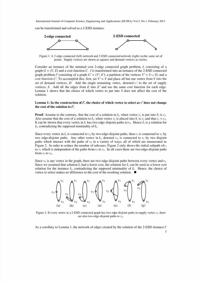
The difference between the two problems is the differentiation of the vertices into supply anddemand vertices which can lead to different solutions as shown in Figure 1. Although the twoproblems are not identical, the 2-edge connected problem can be used to explain that the 2-ESDconnected problem is NP-hard by showing that an instance of the 2-edge connectivity problem




3

can be transformed and solved as a 2-ESD instance.

Figure 1. A 2-edge connected (left) network and 2-ESD connected network (right) on the same set of points. Supply vertices are shown as squares and demand vertices as circles.

Consider an instance of the minimal cost 2-edge connected graph problem, I , consisting of agraph G = (V , E ) and a cost function C . I is transformed into an instance of the 2-ESD connected

graph problem I consisting of a graph G = (V , E ), a partition of the vertices V = S ∪ D, and a

cost function C . To accomplish this, first, set V = V and place all but one vertex from V into the

set of demand vertices, D. Add the single remaining vertex, denoted v , to the set of supply

vertices, S . Add all the edges from E into E and use the same cost function for each edge.Lemma 1 shows that the choice of which vertex to put into S does not affect the cost of thesolution.

Lemma 1: In the construction of I , the choice of which vertex to select as v does not change

the cost of the solution to I .

Proof : Assume to the contrary, that the cost of a solution to I 1, when vertex v1 is put into S , is c1.Also assume that the cost of a solution to I 2, when vertex v2 is placed into S , is c2 and that c1 < c2.It can be shown that every vertex in I 1 has two edge-disjoint paths to v2. Hence I 1 is a solution for I 2, contradicting the supposed minimality of I 2.

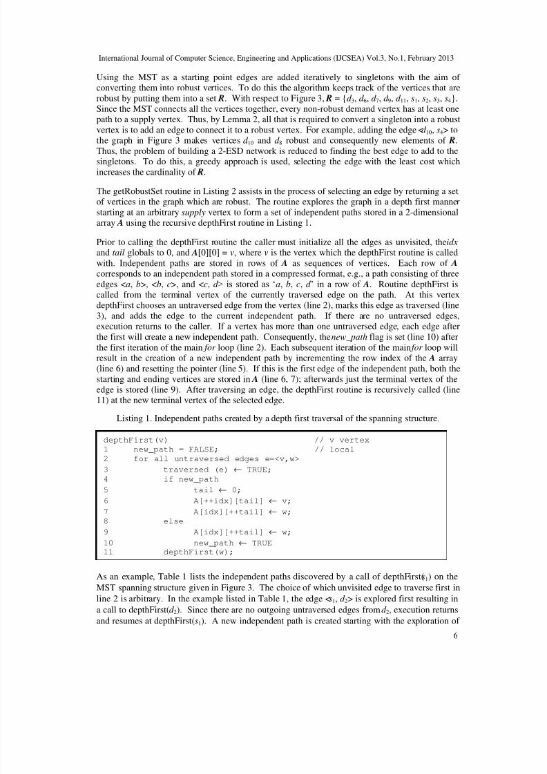
Since every vertex in I 1 is connected to v1 by two edge-disjoint paths, then v2 is connected to v1 bytwo edge-disjoint paths. Any other vertex in I 1, denoted v3, is connected to v1 by two disjointpaths which interact with the paths of v2 in a variety of ways, all of which are enumerated inFigure 2. In order to reduce the number of subcases, Figure 2 only shows the initial subpath of v3

to v1 which is independent of the paths from v2 to v1. In all cases there are two edge-disjoint pathsfrom v3 to v2.

Since v3 is any vertex in the graph, there are two edge-disjoint paths between every vertex and v2.Since we assumed that solution I 1 had a lower cost, the solution for I 1 can be used as a lower costsolution for the instance I 2, contradicting the supposed minimality of I 2. Hence, the choice of vertex to select makes no difference to the cost of the resulting solution.

Figure 2. If every vertex in a 2-ESD connected graph has two edge-disjoint paths to supply vertex v1, thereare also two edge-disjoint paths to v2.

As a corollary to Lemma 1, the network of edges created by the solution of the 2-ESD instance I

(a) (b) (d) (e)

v1

v2

v3

v1

v2

v3 v3

v1

v2

v3

v1

v2

v1

v2

v3

v1

v2

v3v3

v1

v2

(c) (f) (g)

2-ESD connected2-edge connected




4

is 2-edge connected because every vertex has two edge-disjoint paths to v2, an arbitrary vertex inthe graph.

Theorem 1: Given a 2-edge connected instance I , create a 2-ESD instance I by placing all but

one vertex in the demand set and the remaining vertex in the supply set. An optimal solution to I

is an optimal solution to I .

Proof: Select an arbitrary vertex as v to be the supply vertex in the 2-ESD instance I anddetermine the optimal solution. Lemma 1 implies that there are two edge-disjoint paths between

any pair of vertices in I , hence is 2-edge connected. Thus, the optimal solution to I cannot cost

more than the optimal solution I , otherwise I could be used as a lower cost solution.

Since the solution I is 2-edge connected it could be used as a solution for I . Thus, the cost for the

solution I cannot be higher than the cost of the solution for I.

Since the solutions I and I cannot cost more than one another, they must have the same cost.

Furthermore, since I has a feasible structure for a solution to I , an optimal solution to the 2-ESD

instance I , is an optimal solution to the 2-edge instance I.

With the solutions of I and I having the same cost, the problem of finding a 2-ESD connectednetwork is at least as difficult as finding the 2-edge connected network. Consequently, the 2-ESDconnected network problem is NP-Hard.

3. ALGORITHM

The heuristic algorithms employed to generate a solution to the 2-ESD problem can be separatedinto two main components, edge generation and edge reduction/refactoring. The routinesdeveloped to assist the edge-generation phase are explained in greater detail, because anyheuristic algorithm which constructs a 2-ESD network incrementally will require similar routines.First, some definitions and properties are presented.

3.1. Definitions and Properties

A path is a sequence of vertices such that there is an edge between consecutive vertices in thesequence. A simple cycle is a path with no repeated edges and vertices other than the starting andending vertices. A vertex is robust if it is a demand vertex that has two or more edge-disjointpaths to a supply vertex, or is a supply vertex. The degree of a vertex v, denoted as deg(v), is thenumber of incident edges of v. A demand vertex with degree one is called a singleton. When thedegree of a vertex is greater than or equal to a value, it is described with a number followed by a“+”. The cost of an edge is the Euclidean distance between the end points. The cost of a network is the sum of the cost of all of its edges.

Lemma 2: A demand vertex v on a path P which begins and ends on robust vertices v r1 and

v r2 is also robust.

Proof : If vr 1 and vr 2 are the same vertex, denoted vr , then v lies on a simple cycle. The vertex v

has two edge-disjoint paths to vr , one traversing the cycle clock-wise and the other counter-clock-wise. The robust vertex vr has two edge disjoint paths to supply vertices s1 and s2 (s1 may be thesame vertex as s2). It is a simple matter to construct two edge-disjoint paths from v to s1 and s2,via vr , using these four edge-disjoint paths.




5

Otherwise, vr 1 and vr 2 are distinct terminals of a path. In this case, the vertex v has at least onepath to a supply vertex formed by traversing the path from v to vr 1 and then onwards to one of vr 1

supply vertices. Assume that v is not robust then v has only one path to a supply vertex through,without loss of generality, vr 1. Since there are no edge disjoint paths from v to a source throughvr 2, then both of the paths from the robust vertex vr 2 to its associated supply vertices must share acommon edge with the path from vr 1 to its supply vertices. This implies that vr 2 is not robust, acontradiction, consequently v is robust.

The 2-ESD network is formed on the set of vertices in the Euclidian plane along with thecorresponding edges between the vertices. The cost of an edge is the Euclidean distance betweenits associated vertices. Since the algorithm spends a significant amount of time processing edges,there is a strong motivation to reduce the size of the pool of O(|V |2) candidate edges.

Call an edge, both of whose terminals are demand vertices, a demand-edge. It can be shown thatin an optimal 2-ESD connected network, demand-edges do not cross. Hence, when connectingdemand vertices, the algorithm only selects non-intersecting edges. To facilitate this selection,the algorithm draws edges from those in the Delaunay triangulation [12,13].

A triangulation of a graph G = (V , E ) is a partitioning of the plane into triangles whose verticesare the vertices of the graph. A Delaunay triangulation consists of the vertices of V along with a

subset of edges E ⊆ E which meet the empty-circle condition [12]. An edge e is said to meet theempty-circle condition if there exists a circle circumscribing the end vertices that does not containany other vertices of the graph. Since the edges of the Delaunay triangulation do not intersect oneanother, they form a convenient set from which to draw candidate edges of the 2-ESD network. Itremains an open question whether an optimal 2-ESD connected network is constructed solelyfrom edges in the Delaunay triangulation. Consequently, restricting an algorithm to this set of edges, while convenient for the formation of a redundant network, may result in a suboptimalsolution.

3.2. Generation of Redundant Edges

The algorithm developed to solve the 2-ESD redundant problem starts by forming a minimumspanning tree (MST) over all the points in the graph making no distinction between the supplyand demand vertices. Figure 3 shows the MST (in bold lines) over an instance with 4 supplyvertices (squares) and 11 demand vertices (circles). The supply and demand vertices are labeledwith an “s” and “d ”, respectively, and subscripted with an index. The edges of the Delaunay

triangulation are the union of the dotted lines and the MST edges. There are five singletons d 1,d 2, d 4, d 5 and d 10.

Figure 3. The MST, built from Delaunay triangulation, for the set of 11 demand vertices and 4 supplyvertices.




6

Using the MST as a starting point edges are added iteratively to singletons with the aim of converting them into robust vertices. To do this the algorithm keeps track of the vertices that arerobust by putting them into a set R. With respect to Figure 3, R = {d 3, d 6, d 7, d 9, d 11, s1, s2, s3, s4}.Since the MST connects all the vertices together, every non-robust demand vertex has at least onepath to a supply vertex. Thus, by Lemma 2, all that is required to convert a singleton into a robustvertex is to add an edge to connect it to a robust vertex. For example, adding the edge <d 10, s4> tothe graph in Figure 3 makes vertices d 10 and d 8 robust and consequently new elements of R.Thus, the problem of building a 2-ESD network is reduced to finding the best edge to add to thesingletons. To do this, a greedy approach is used, selecting the edge with the least cost whichincreases the cardinality of R.

The getRobustSet routine in Listing 2 assists in the process of selecting an edge by returning a setof vertices in the graph which are robust. The routine explores the graph in a depth first mannerstarting at an arbitrary supply vertex to form a set of independent paths stored in a 2-dimensionalarray A using the recursive depthFirst routine in Listing 1.

Prior to calling the depthFirst routine the caller must initialize all the edges as unvisited, the idx

and tail globals to 0, and A[0][0] = v, where v is the vertex which the depthFirst routine is calledwith. Independent paths are stored in rows of A as sequences of vertices. Each row of A

corresponds to an independent path stored in a compressed format, e.g., a path consisting of threeedges <a, b>, <b, c>, and <c, d > is stored as ‘a, b, c, d ’ in a row of A. Routine depthFirst iscalled from the terminal vertex of the currently traversed edge on the path. At this vertexdepthFirst chooses an untraversed edge from the vertex (line 2), marks this edge as traversed (line3), and adds the edge to the current independent path. If there are no untraversed edges,execution returns to the caller. If a vertex has more than one untraversed edge, each edge afterthe first will create a new independent path. Consequently, the new_path flag is set (line 10) afterthe first iteration of the main for loop (line 2). Each subsequent iteration of the main for loop willresult in the creation of a new independent path by incrementing the row index of the A array(line 6) and resetting the pointer (line 5). If this is the first edge of the independent path, both thestarting and ending vertices are stored in A (line 6, 7); afterwards just the terminal vertex of theedge is stored (line 9). After traversing an edge, the depthFirst routine is recursively called (line11) at the new terminal vertex of the selected edge.

Listing 1. Independent paths created by a depth first traversal of the spanning structure.

As an example, Table 1 lists the independent paths discovered by a call of depthFirst(s1) on the

MST spanning structure given in Figure 3. The choice of which unvisited edge to traverse first in

line 2 is arbitrary. In the example listed in Table 1, the edge <s1, d 2> is explored first resulting in

a call to depthFirst(d 2). Since there are no outgoing untraversed edges from d 2, execution returns

and resumes at depthFirst(s1). A new independent path is created starting with the exploration of

depthFirst(v) // v vertex

1 new_path = FALSE; // local

2 for all untraversed edges e=<v,w>

3 traversed (e) ← TRUE;

4 if new_path

5 tail ← 0;

6 A[++idx][tail] ← v;

7 A[idx][++tail] ← w;

8 else

9 A[idx][++tail] ← w;

10 new_path ← TRUE11 depthFirst(w);




7

edge <s1, d 3> and a commensurate call to depthFirst(d 3). Notice that the last vertex in eachindependent path has degree one and consequently is a singleton if it is a demand vertex.

Table 1. Six independent paths for the MST inFigure 3 derived by depthFirst called with the supply vertex s1.

Independent Paths in A1 s1, d 22 s1, d 3, d 13 d 3, s2, d 44 s2, d 6, d 9, s4, d 11, d 7, s3

5 d 7, d 56 d 9, d 8, d 10

The time complexity of the depthFirst routine is simple to compute. The routine visits each of theO(|V |) edges in the spanning structure once and does a constant amount of work at each. Hencethe running time of the depthFirst routine is O(|V |).

To understand the behavior of getRobustSet it is necessary to understand the context in which it iscalled. As previously described the MST is augmented with edges until all the vertices arerobust. After each edge is added to a singleton, getRobustSet is called and returns the new set of robust vertices.

Listing 2. The get RobustSet routine is called after every single edge insertion.

getRobustSet(s) // s ∈ S, the set of supply vertices

1. A ← depthFirst(s);

2. tail ← length(A[0])-1;

3. for i ←0 to length(A)-1

4. Q[i] ← A[0][i];

5. for i ← 1 to length(A)-1

6. robust ← false;7. while Q[tail] != A[i][0]

8. if Q[tail] ∈ S || Q[tail] ∈ R

9. robust ← true;

10. if robust = true && Q[tail] ∉ R

11. R ← R ∪ Q[tail];

12. tail ← tail - 1;


14. R ← R ∪ Q[tail];

15. for j ← 0 to length(A[i])-1

16. tail ← tail + 1;

17. Q[tail] ← A[i][j];

18. robust ← false;

19. while tail >= 0

20. if Q[tail] ∈ S || Q[tail] ∈ R

21. robust ← true;


23. R ← R ∪ Q[tail];

24. tail ← tail - 1;

25. return R;




8

As seen in Listing 2, getRobustSet calls depthFirst, with an arbitrary supply vertex s. After thedepthFirst determines the set of independent paths in the spanning structure, the getRobustroutine will utilize these independent paths to construct paths, all rooted at s, through thespanning structure.

The current path through the spanning structure is maintained in an array Q. The first element of Q will always be s, a supply vertex used in the call to depthFirst. The getRobustSet routineinitializes the path of vertices, Q, to the first independent path discovered by the depthFirstroutine (lines 3-4). Next, getRobustSet backward scans the Q array from the last element towardsthe first element, and looks for a robust vertex, stopping only when it finds the first element of thenext independent path in A (line 7). Since the path implied by Q is always rooted at a supplyvertex, any robust vertex encountered will, by Lemma 2, result in all of the vertices between therobust vertex and s being classified as robust. However, this conversion will not happen all atonce in the getRobustSet routine. When a robust vertex is encountered (lines 8) the robust flag isset (line 9) and the vertices in Q, up to the first vertex of the next independent path in A, are thenmoved into R (lines 10, 11 and 13, 14). The next independent path is then appended to Q (lines15-17). After the last independent path in A has been appended, the backward scan of Q iscontinued all the way back to s, the argument of getRobustSet (lines 19-24).

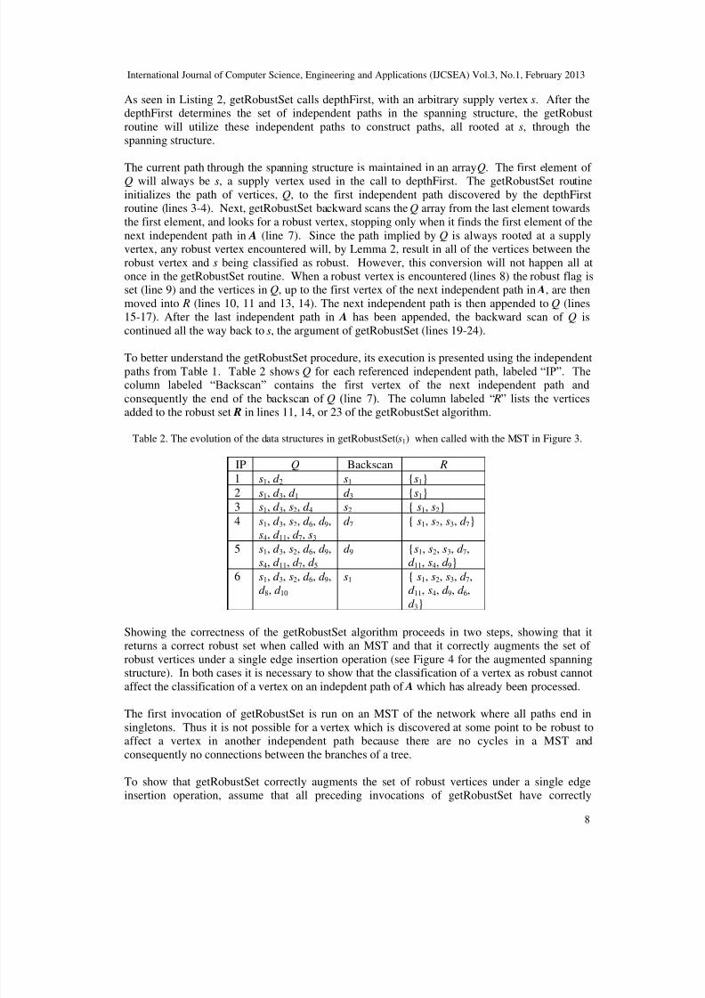
To better understand the getRobustSet procedure, its execution is presented using the independentpaths from Table 1. Table 2 shows Q for each referenced independent path, labeled “IP”. Thecolumn labeled “Backscan” contains the first vertex of the next independent path and

consequently the end of the backscan of Q (line 7). The column labeled “ R” lists the vertices

added to the robust set R in lines 11, 14, or 23 of the getRobustSet algorithm.

Table 2. The evolution of the data structures in getRobustSet(s1) when called with the MST in Figure 3.

IP Q Backscan R

1 s1, d 2 s1 {s1}2 s1, d 3, d 1 d 3 {s1}3 s1, d 3, s2, d 4 s2 { s1, s2}

4 s1, d 3, s2, d 6, d 9,s4, d 11, d 7, s3d 7 { s1, s2, s3, d 7}

5 s1, d 3, s2, d 6, d 9,s4, d 11, d 7, d 5

d 9 {s1, s2, s3, d 7,d 11, s4, d 9}

6 s1, d 3, s2, d 6, d 9,d 8, d 10

s1 { s1, s2, s3, d 7,d 11, s4, d 9, d 6,d 3}

Showing the correctness of the getRobustSet algorithm proceeds in two steps, showing that itreturns a correct robust set when called with an MST and that it correctly augments the set of robust vertices under a single edge insertion operation (see Figure 4 for the augmented spanningstructure). In both cases it is necessary to show that the classification of a vertex as robust cannotaffect the classification of a vertex on an indepdent path of A which has already been processed.

The first invocation of getRobustSet is run on an MST of the network where all paths end insingletons. Thus it is not possible for a vertex which is discovered at some point to be robust toaffect a vertex in another independent path because there are no cycles in a MST andconsequently no connections between the branches of a tree.

To show that getRobustSet correctly augments the set of robust vertices under a single edgeinsertion operation, assume that all preceding invocations of getRobustSet have correctly




9

identified the set of robust vertices. An edge is added to the spanning structure from a singletonvertex, v, to a redundant vertex, w. After the edge, e = < v, w>, is added to the spanning structure,getRedundentSet is called to augment the robust set. The edge <v, w> will cause the vertices onthe path from s to v to become robust. No other vertices in the spanning structure are affectedbecause w is already robust and there is at most one path from v to s (that’s why v is a singleton).

Figure 4. The spanning structure resulting from the edge augmentation of the MST in Figure 3.

There are times when the set of edges provided by the Delaunay triangulation proves to beinsufficient for the augmentation process to find an edge which increases the size of the robustvertices as shown in Figure 5. In such cases the augmentation algorithm looks for the shortestedge which connects the singleton to a supply vertex.

Figure 5. Example of a 2-ESD connectivity which uses an edge outside of the Delaunay triangulation.

The augmentation process ends when the set of robust vertices is equal to the set of supply anddemand vertices. At this point the graph is 2-ESD connected. The second phase of the algorithmsthen takes over, reducing the cost of the 2-ESD connected network while maintaining theredundancy of the network.

3.3. Edge Reduction/Refactoring

The graph resulting from the augmentation of the MST is 2-ESD connected, but may not beoptimal in terms of cost. The cost of the spanning structure can be reduced by eliminating

unnecessary edges using reduction heuristics. The removal of an edge may have two negativeconsequences, eliminating the robustness of a vertex or breaking the graph into two components.In order to ensure that the application of a reduction heuristic does not create an illegalconfiguration, the edge replacement is applied only if getRobustSet returns a complete set of vertices under a tentative application of the edge reduction. The three reduction heuristicsutilized are greedy-based and often yield a solution that is close to optimal.




10

3.3.1. Triangle Inequality

The first reduction heuristic looks to replace a pair of edges with a single edge based on thetriangle inequality. A 2-ESD redundant network containing a supply vertex with degree 3+ or ademand vertex with degree 4+ can have its cost reduced by replacing the two most expensiveedges <v, v1> and <v, v2> with the edge <v1, v2> where v is the high degree vertex. Thisreplacement always reduces the cost of the network because the triangle inequality states that thesum of any two edges of a triangle is always greater than the length of the third edge [12].

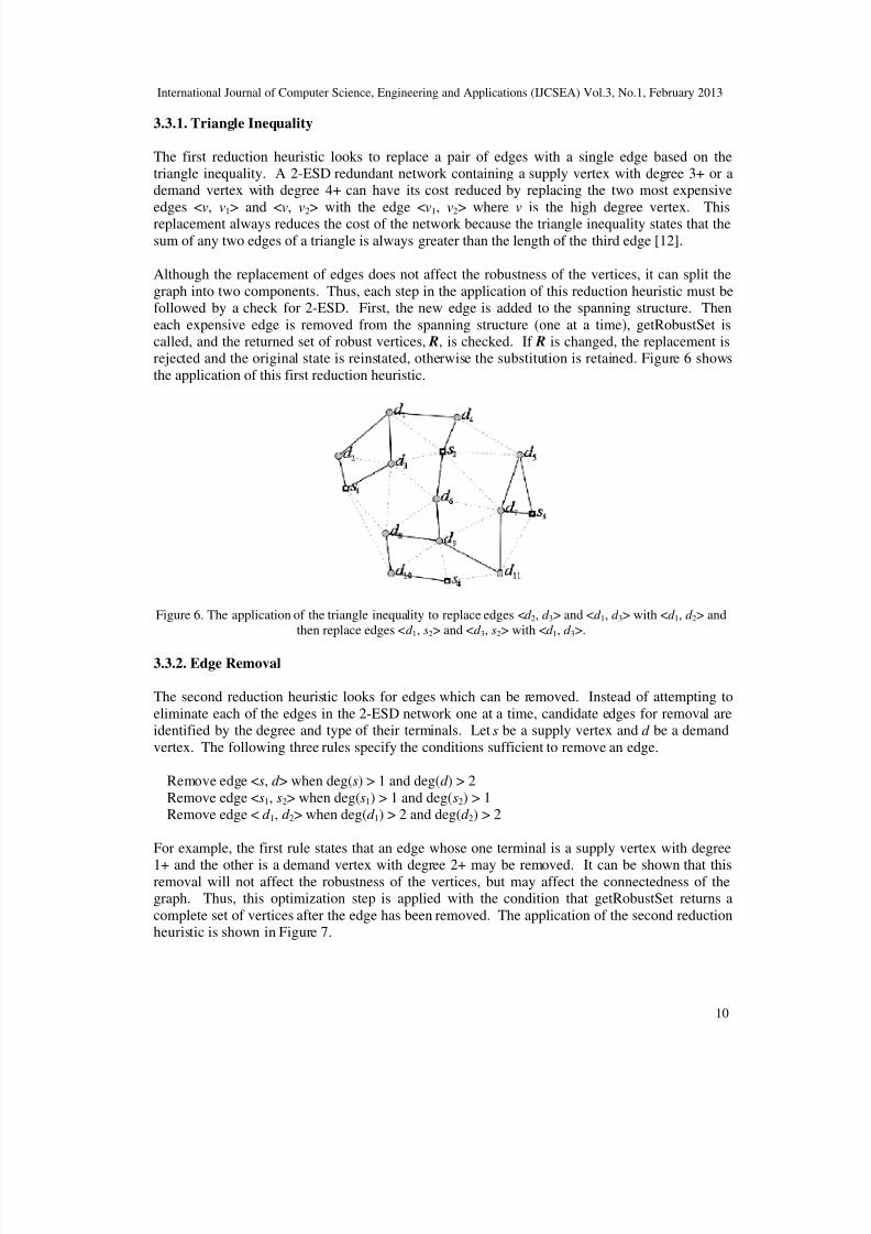
Although the replacement of edges does not affect the robustness of the vertices, it can split thegraph into two components. Thus, each step in the application of this reduction heuristic must befollowed by a check for 2-ESD. First, the new edge is added to the spanning structure. Theneach expensive edge is removed from the spanning structure (one at a time), getRobustSet iscalled, and the returned set of robust vertices, R, is checked. If R is changed, the replacement isrejected and the original state is reinstated, otherwise the substitution is retained. Figure 6 showsthe application of this first reduction heuristic.

Figure 6. The application of the triangle inequality to replace edges <d 2, d 3> and <d 1, d 3> with <d 1, d 2> andthen replace edges <d 1, s2> and <d 3, s2> with <d 1, d 3>.

3.3.2. Edge Removal

The second reduction heuristic looks for edges which can be removed. Instead of attempting toeliminate each of the edges in the 2-ESD network one at a time, candidate edges for removal areidentified by the degree and type of their terminals. Let s be a supply vertex and d be a demandvertex. The following three rules specify the conditions sufficient to remove an edge.

Remove edge <s, d > when deg(s) > 1 and deg(d ) > 2Remove edge <s1, s2> when deg(s1) > 1 and deg(s2) > 1Remove edge < d 1, d 2> when deg(d 1) > 2 and deg(d 2) > 2

For example, the first rule states that an edge whose one terminal is a supply vertex with degree

1+ and the other is a demand vertex with degree 2+ may be removed. It can be shown that thisremoval will not affect the robustness of the vertices, but may affect the connectedness of thegraph. Thus, this optimization step is applied with the condition that getRobustSet returns acomplete set of vertices after the edge has been removed. The application of the second reductionheuristic is shown in Figure 7.




11

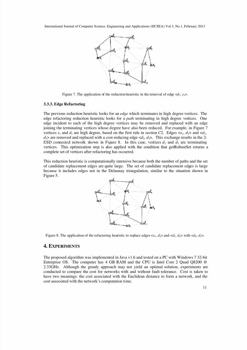
Figure 7. The application of the reduction heuristic in the removal of edge <d 7, s3>.

3.3.3. Edge Refactoring

The previous reduction heuristic looks for an edge which terminates in high degree vertices. Theedge refactoring reduction heuristic looks for a path terminating in high degree vertices. One

edge incident to each of the high degree vertices may be removed and replaced with an edge joining the terminating vertices whose degree have also been reduced. For example, in Figure 7vertices s1 and d 1 are high degree, based on the first rule in section C 2. Edges <s1, d 3> and <d 1,d 2> are removed and replaced with a cost-reducing edge <d 2, d 3>. This exchange results in the 2-ESD connected network shown in Figure 8. In this case, vertices d 2 and d 3 are terminatingvertices. This optimization step is also applied with the condition that getRobustSet returns acomplete set of vertices after refactoring has occurred.

This reduction heuristic is computationally intensive because both the number of paths and the setof candidate replacement edges are quite large. The set of candidate replacement edges is largebecause it includes edges not in the Delaunay triangulation, similar to the situation shown inFigure 5.

Figure 8. The application of the refactoring heuristic to replace edges <s1, d 3> and <d 1, d 2> with <d 2, d 3>.

4. EXPERIMENTS

The proposed algorithm was implemented in Java v1.6 and tested on a PC with Windows 7 32-bitEnterprise OS. The computer has 4 GB RAM and the CPU is Intel Core 2 Quad Q8200 @2.33GHz. Although the greedy approach may not yield an optimal solution, experiments areconducted to compare the cost for networks with and without fault tolerance. Cost is taken tohave two meanings: the cost associated with the Euclidean distance to form a network, and thecost associated with the network’s computation time.




12

To address different network complexities, the number of vertices in the network covers 10, 50,100 and then increments by 100 up to 800 vertices. Coordinates are randomly generated within a600 × 1000 rectangle. The density of demand vertices, with respect to the number of vertices, isvaried between 10% and 90%. Note that a density of 0% implies that all the vertices are supplyvertices. Consequently the connection requirements of the supply vertices imply that the 2-ESDnetwork is simply an MST.

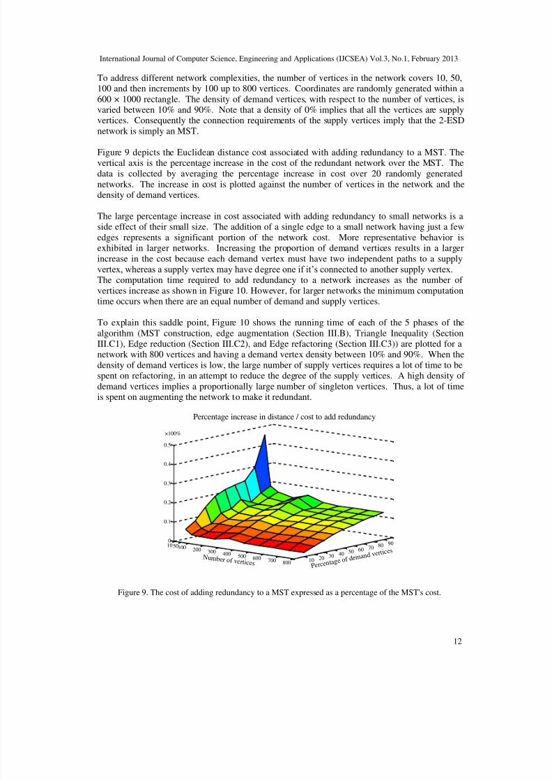
Figure 9 depicts the Euclidean distance cost associated with adding redundancy to a MST. Thevertical axis is the percentage increase in the cost of the redundant network over the MST. Thedata is collected by averaging the percentage increase in cost over 20 randomly generatednetworks. The increase in cost is plotted against the number of vertices in the network and thedensity of demand vertices.

The large percentage increase in cost associated with adding redundancy to small networks is aside effect of their small size. The addition of a single edge to a small network having just a fewedges represents a significant portion of the network cost. More representative behavior isexhibited in larger networks. Increasing the proportion of demand vertices results in a largerincrease in the cost because each demand vertex must have two independent paths to a supply

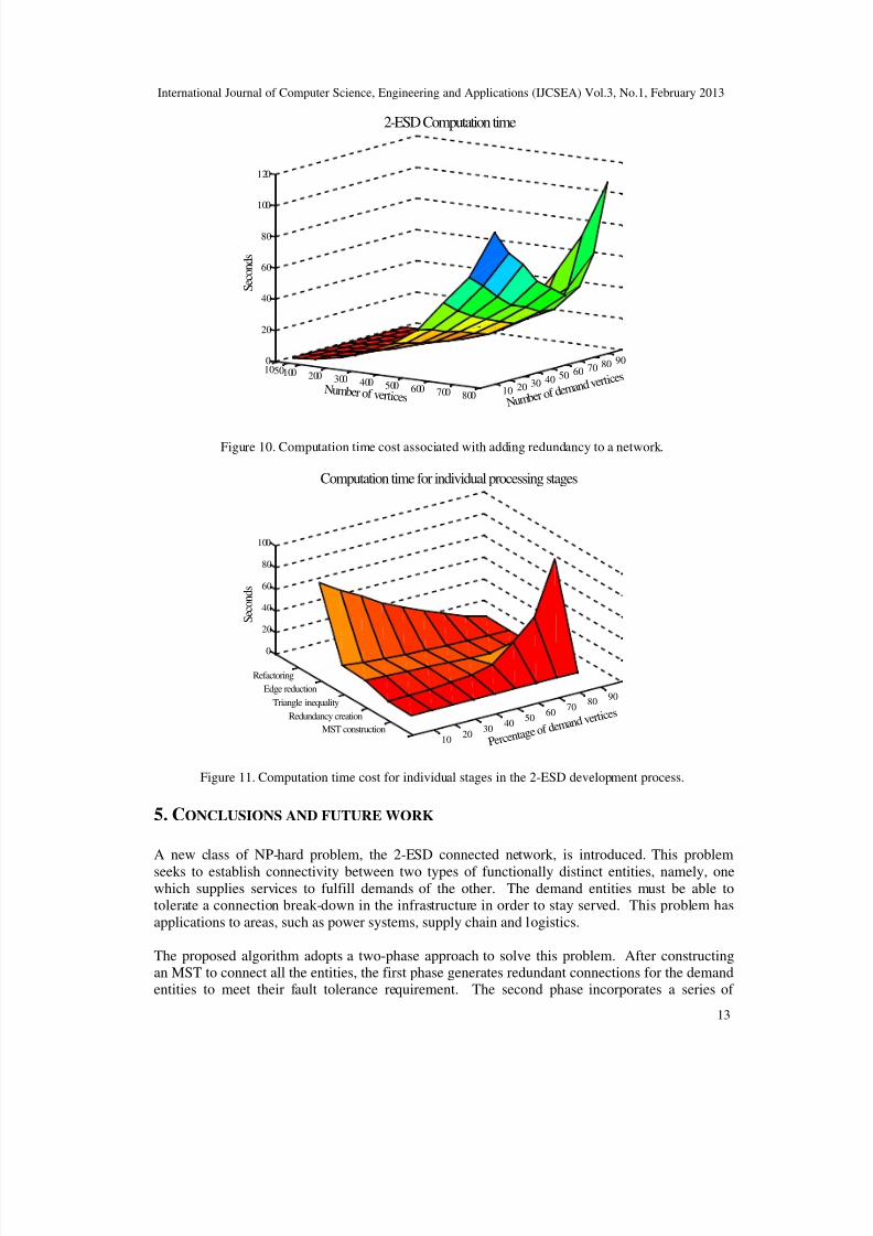
vertex, whereas a supply vertex may have degree one if it’s connected to another supply vertex.The computation time required to add redundancy to a network increases as the number of vertices increase as shown in Figure 10. However, for larger networks the minimum computationtime occurs when there are an equal number of demand and supply vertices.

To explain this saddle point, Figure 10 shows the running time of each of the 5 phases of thealgorithm (MST construction, edge augmentation (Section III.B), Triangle Inequality (SectionIII.C1), Edge reduction (Section III.C2), and Edge refactoring (Section III.C3)) are plotted for anetwork with 800 vertices and having a demand vertex density between 10% and 90%. When thedensity of demand vertices is low, the large number of supply vertices requires a lot of time to bespent on refactoring, in an attempt to reduce the degree of the supply vertices. A high density of demand vertices implies a proportionally large number of singleton vertices. Thus, a lot of timeis spent on augmenting the network to make it redundant.

1050100 200 300 400 500 600 700 800 10 20 30 40 50 60 70 8090

0

0.1

0.2

0.3

0.4

0.5

P e r c e n t ag e o f

d e m a n d v e r t i

c e s

Percentage increase in distance / cost to add redundancy

N umb er o f v er t ices

×100%

Figure 9. The cost of adding redundancy to a MST expressed as a percentage of the MST's cost.




13

1050100 200 300 400 500 600 700 800 10 20 30 40 50 60 70 80 900

20

40

60

80

100

120

N u m b e r o f d e

m a n d v e r t i c e s

2-ESD Computation time

N umber o f v er t ices

S e c o n

d s

Figure 10. Computation time cost associated with adding redundancy to a network.

1020

3040

5060

7080

90

MST construction

Redundancy creation

Triangle inequality

Edge reduction

Refactoring

0

20

40

60

80

100

P e r c e n t ag e o f

d e m a n d v e r t i

c e s

Computation time for individual processing stages

S e c o n

d s

Figure 11. Computation time cost for individual stages in the 2-ESD development process.

5. CONCLUSIONS AND FUTURE WORK

A new class of NP-hard problem, the 2-ESD connected network, is introduced. This problem

seeks to establish connectivity between two types of functionally distinct entities, namely, onewhich supplies services to fulfill demands of the other. The demand entities must be able totolerate a connection break-down in the infrastructure in order to stay served. This problem hasapplications to areas, such as power systems, supply chain and logistics.

The proposed algorithm adopts a two-phase approach to solve this problem. After constructingan MST to connect all the entities, the first phase generates redundant connections for the demandentities to meet their fault tolerance requirement. The second phase incorporates a series of




14

greedy procedures to refactor and eliminate unnecessary connections to decrease the cost of theentire infrastructure. Experimental results show that adding redundancy may increase the cost of the infrastructure by up to 20% for large network.

Future work in this area includes looking at more effective optimization heuristics whiledecreasing the running time of the algorithm. Since the luxury of designing a new network topology from scratch is rare, there is a need to examine how to augment an existing non-redundant network to make it redundant. A related problem is how to add supply and demandvertices and edges to an existing network so that the connection requirements of a 2-ESD network are satisfied.

This work considers space to have a uniform cost. In some applications this may not be the case,for example when installing transmission lines the cost to traverse an open plain may be greaterthan when traversing a mountainous regions. Further work needs to be directed at this practicalvariation.

REFERENCES

[1] Brown, R., Electric Power Distribution Reliability, 2nd Ed., CRC Press, 2009.[2] Pourbeik, P.; Kundur, P.S.; and Taylor, C.W.; , “The anatomy of a power grid blackout - Root causes

and dynamics of recent major blackouts,” Power and Energy Magazine, IEEE , vol.4, no.5, pp.22-29,Sept.-Oct. 2006.

[3] ERCOT System Planning Study, “Competitive Renewable Energy Zones (CR EZ) TransmissionOptimization Study,” April 2, 2008.

[4] Wada, K.; Luo, Y.; and Kawaguchi, K., “Optimal Fault-Tolerant Routings for Connected Graphs,”

Information Processing Letters, Vol. 41, Iss. 3, Mar. 1992, pp. 169 – 174.[5] Liu, Y. L.; and Wang, Y-L.; Guan, D.J.; "An optimal fault-tolerant routing algorithm for double-loop

networks," Computers, IEEE Transactions on, vol.50, no.5, pp.500-505, May 2001.[6] Moraes, R.E.N.; Ribeiro, C.C.; Duhamel, C.; , "Optimal solutions for fault-tolerant topology control

in wireless ad hoc networks," Wireless Communications, IEEE Transactions on , vol.8, no.12,pp.5970-5981, December 2009.

[7] Cheng, L.; Carter, J.; and Dai, D., “An Adaptive Cache Coherence Protocol Optimized for Producer -

Consumer Sharing”, IEEE 13th International Symposium on High Performance ComputerArchitecture, Scottsdale, AZ, pp. 328 – 339, February 2007.

[8] Hou, P.; and Hsu, Y., “Finding Dominant Links of Emergency Network with Respect to Earthquake

Disaster,” Journal of the Eastern Asia Society for Transportation Studies, Vol. 6, pp. 77 - 90, 2005.[9] Papadimitriou C.; and Steiglitz K., Combinatorial Optimization Algorithms and Complexity. Mineola,

New York: Dover Publications, 1998.[10] A Computational Investigation of Heuristic Algorithms for 2-edge-Connectivity Augmentation,

Jørgen Bang-Jensen, Marco Chiarandini *, Peter Morling, Networks, Volume 55 Issue 4, Pages 299 –

325.[11] Garey, M.R.; and Johnson D.S. (1979). Computers and Intractability: A Guide to the Theory of NP-

Completeness. W.H. Freeman.[12] O’Rourke, J., Computational Geometry in C, Cambridge University Press, 2000.

[13] Berg, M.D.; Cheong, O.; Kreveld, M.V., Overmars M., Computational Geometry: Algorithms andApplications, Springer, Nov. 19, 2010.




15

AUTHORS

Dr. Wang received his Ph.D. in Computer Science from State University of New York atAlbany in 2002. He is currently an Associate Professor in Computer Science andSoftware Engineering department at Penn State Erie, The Behrend College. His researchinterests are in software design, software architecture, software reliability, pattern

recognition, machine learning, adaptive systems, and game AIs.

Dr. Chris Coulston received his B.A. in Physics in 1989 from Slippery Rock University,his B.S. 1991, the M.S. 1994 and the Ph.D. 1999 in Computer Engineering, all from thePennsylvania State University. Dr. Coulston taught at the University Park campus from1993-1998. He is chair of the Computer Science and Software Engineering Departmentbeginning January 2012. He was the former chair of Electrical, Computer, and SoftwareEngineering programs. He received the best paper award for Constructing ExactOoctagonal Steiner Minimal Trees, at the Great Lakes Symposium on Circuits andSystems, April 2003 and co-authored Design for Electrical and Computer Engineers: Theory, Concepts andPractice. New York: McGraw-Hill Higher Education, 2005, 300 pp., ISBN 0-07-319599-5 with Dr. RalphFord, director of the School of Engineering.

Dr. Robert Weissbach is currently an associate professor of engineering at Penn State

Erie, The Behrend College. From October 2007 through June 2008, he was a visitingresearcher at Aalborg University in Aalborg, Denmark. His research interests are inrenewable energy, energy storage, power electronics and power systems.

Dr. Tang received her Ph.D. in Computer Science from SUNY Albany in 2003. She iscurrently an Associate Professor in Computer and Information Science department atGannon University. Her research interests are in software design, software metrics,software architecture, software reliability, software testing, and swarm intellige

Connecting Supply and Demand Vertices with Fault Tolerance

Documents

Transcript of Connecting Supply and Demand Vertices with Fault Tolerance