Conjugate Gradient Method - Stanford University• incomplete/approximate Cholesky factorization:...

Conjugate Gradient Method

• direct and indirect methods

• positive definite linear systems

• Krylov sequence

• spectral analysis of Krylov sequence

• preconditioning

EE364b, Stanford University

Three classes of methods for linear equations

methods to solve linear system Ax = b, A ∈ Rn×n

• dense direct (factor-solve methods)

– runtime depends only on size; independent of data, structure, orsparsity

– work well for n up to a few thousand

• sparse direct (factor-solve methods)

– runtime depends on size, sparsity pattern; (almost) independent ofdata

– can work well for n up to 104 or 105 (or more)– requires good heuristic for ordering

EE364b, Stanford University 1

• indirect (iterative methods)

– runtime depends on data, size, sparsity, required accuracy– requires tuning, preconditioning, . . .– good choice in many cases; only choice for n = 106 or larger


Symmetric positive definite linear systems

SPD system of equations

Ax = b, A ∈ Rn×n, A = AT ≻ 0

examples

• Newton/interior-point search direction: ∇2φ(x)∆x = −∇φ(x)

• least-squares normal equations: (ATA)x = AT b

• regularized least-squares: (ATA+ µI)x = AT b

• minimization of convex quadratic function (1/2)xTAx− bTx

• solving (discretized) elliptic PDE (e.g., Poisson equation)


• analysis of resistor circuit: Gv = i

– v is node voltage (vector), i is (given) source current– G is circuit conductance matrix

Gij =

{

total conductance incident on node i i = j−(conductance between nodes i and j) i 6= j


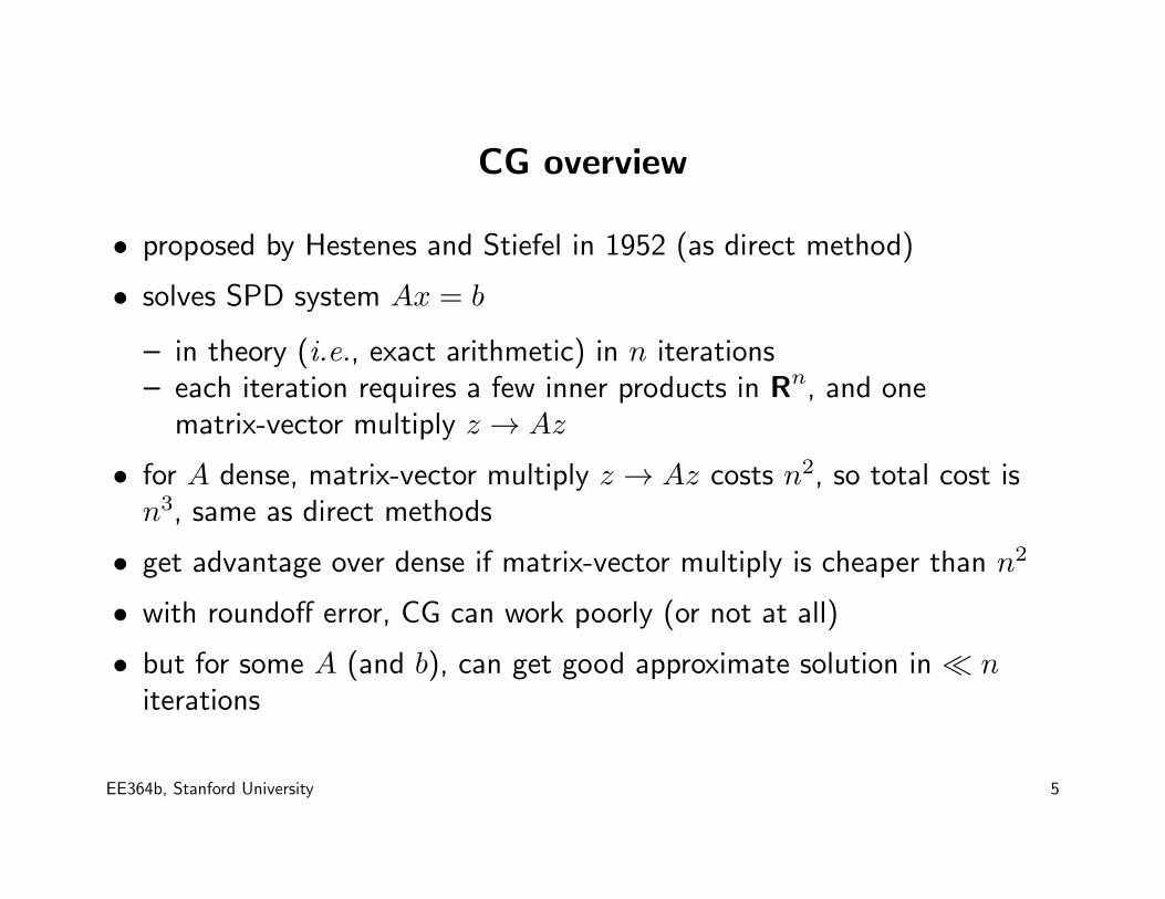
CG overview

• proposed by Hestenes and Stiefel in 1952 (as direct method)

• solves SPD system Ax = b

– in theory (i.e., exact arithmetic) in n iterations– each iteration requires a few inner products in Rn, and one

matrix-vector multiply z → Az

• for A dense, matrix-vector multiply z → Az costs n2, so total cost isn3, same as direct methods

• get advantage over dense if matrix-vector multiply is cheaper than n2

• with roundoff error, CG can work poorly (or not at all)

• but for some A (and b), can get good approximate solution in ≪ niterations


Solution and error

• x⋆ = A−1b is solution

• x⋆ minimizes (convex function) f(x) = (1/2)xTAx− bTx

• ∇f(x) = Ax− b is gradient of f

• with f⋆ = f(x⋆), we have

f(x)− f⋆ = (1/2)xTAx− bTx− (1/2)x⋆TAx⋆ + bTx⋆

= (1/2)(x− x⋆)TA(x− x⋆)

= (1/2)‖x− x⋆‖2A

i.e., f(x)− f⋆ is half of squared A-norm of error x− x⋆


• a relative measure (comparing x to 0):

τ =f(x)− f⋆

f(0)− f⋆=

‖x− x⋆‖2A‖x⋆‖2A

(fraction of maximum possible reduction in f , compared to x = 0)


Residual

• r = b−Ax is called the residual at x

• r = −∇f(x) = A(x⋆ − x)

• in terms of r, we have

f(x)− f⋆ = (1/2)(x− x⋆)TA(x− x⋆)

= (1/2)rTA−1r

= (1/2)‖r‖2A−1

• a commonly used measure of relative accuracy: η = ‖r‖/‖b‖

• τ ≤ κ(A)η2 (η is easily computable from x; τ is not)


Krylov subspace

(a.k.a. controllability subspace)

Kk = span{b, Ab, . . . , Ak−1b}= {p(A)b | p polynomial, deg p < k}

we define the Krylov sequence x(1), x(2), . . . as

x(k) = argminx∈Kk

f(x) = argminx∈Kk

‖x− x⋆‖2A

the CG algorithm (among others) generates the Krylov sequence


Properties of Krylov sequence

• f(x(k+1)) ≤ f(x(k)) (but ‖r‖ can increase)

• x(n) = x⋆ (i.e., x⋆ ∈ Kn even when Kn 6= Rn)

• x(k) = pk(A)b, where pk is a polynomial with deg pk < k

• less obvious: there is a two-term recurrence

x(k+1) = x(k) + αkr(k) + βk(x

(k) − x(k−1))

for some αk, βk (basis of CG algorithm)


Cayley-Hamilton theorem

characteristic polynomial of A:

χ(s) = det(sI −A) = sn + α1sn−1 + · · ·+ αn

by Caley-Hamilton theorem

χ(A) = An + α1An−1 + · · ·+ αnI = 0

and so

A−1 = −(1/αn)An−1 − (α1/αn)A

n−2 − · · · − (αn−1/αn)I

in particular, we see that x⋆ = A−1b ∈ Kn


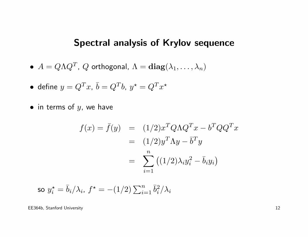
Spectral analysis of Krylov sequence

• A = QΛQT , Q orthogonal, Λ = diag(λ1, . . . , λn)

• define y = QTx, b = QT b, y⋆ = QTx⋆

• in terms of y, we have

f(x) = f(y) = (1/2)xTQΛQTx− bTQQTx

= (1/2)yTΛy − bTy

=

n∑

i=1

(

(1/2)λiy2i − biyi

)

so y⋆i = bi/λi, f⋆ = −(1/2)

∑ni=1 b

2i/λi


Krylov sequence in terms of y

y(k) = argminy∈Kk

f(y), Kk = span{b,Λb, . . . ,Λk−1b}

y(k)i = pk(λi)bi, deg pk < k

pk = argmindeg p<k

n∑

i=1

b2i(

(1/2)λip(λi)2 − p(λi)

)


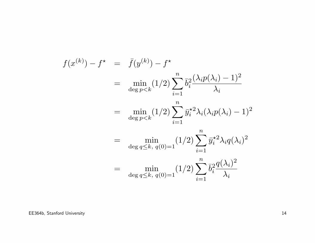
f(x(k))− f⋆ = f(y(k))− f⋆

= mindeg p<k

(1/2)

n∑

i=1

b2i(λip(λi)− 1)2

λi

= mindeg p<k

(1/2)n∑

i=1

y⋆2i λi(λip(λi)− 1)2

= mindeg q≤k, q(0)=1

(1/2)

n∑

i=1

y⋆2i λiq(λi)2

= mindeg q≤k, q(0)=1

(1/2)

n∑

i=1

b2iq(λi)

2

λi


τk =mindeg q≤k, q(0)=1

∑ni=1 y

⋆2i λiq(λi)

2

∑ni=1 y

⋆2i λi

≤ mindeg q≤k, q(0)=1

(

maxi=1,...,n

q(λi)2

)

• if there is a polynomial q of degree k, with q(0) = 1, that is small onthe spectrum of A, then f(x(k))− f⋆ is small

• if eigenvalues are clustered in k groups, then y(k) is a good approximatesolution

• if solution x⋆ is approximately a linear combination of k eigenvectors ofA, then y(k) is a good approximate solution


A bound on convergence rate

• taking q as Chebyshev polynomial of degree k, that is small on interval[λmin, λmax], we get

τk ≤(√

κ− 1√κ+ 1

)k

, κ = λmax/λmin

• convergence can be much faster than this, if spectrum of A is spreadbut clustered


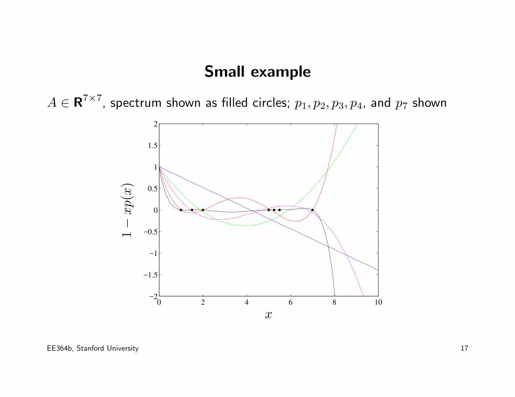
Small example

A ∈ R7×7, spectrum shown as filled circles; p1, p2, p3, p4, and p7 shown

0 2 4 6 8 10−2

−1.5

−1

−0.5

0

0.5

1

1.5

2

x

1−

xp(x)


Convergence

0 1 2 3 4 5 6 70

0.1

0.2

0.3

0.4

0.5

0.6

0.7

0.8

0.9

1

k

τ k


Residual convergence

0 1 2 3 4 5 6 70

0.1

0.2

0.3

0.4

0.5

0.6

0.7

0.8

0.9

1

k

η k


Larger example

• solve Gv = i, resistor network with 105 nodes

• average node degree 10; around 106 nonzeros in G

• random topology with one grounded node

• nonzero branch conductances uniform on [0, 1]

• external current i uniform on [0, 1]

• sparse Cholesky factorization of G requires too much memory


Residual convergence

0 10 20 30 40 50 6010

−8

10−6

10−4

10−2

100

102

104

k

η k


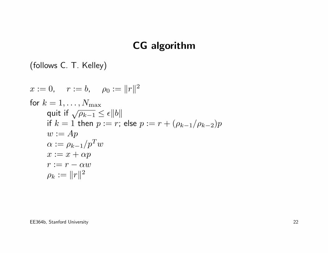
CG algorithm

(follows C. T. Kelley)

x := 0, r := b, ρ0 := ‖r‖2

for k = 1, . . . , Nmax

quit if√ρk−1 ≤ ǫ‖b‖

if k = 1 then p := r; else p := r + (ρk−1/ρk−2)pw := Apα := ρk−1/p

Twx := x+ αpr := r − αwρk := ‖r‖2


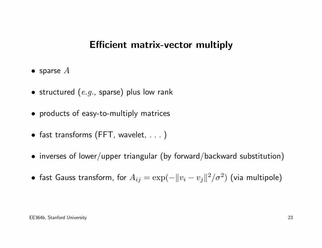
Efficient matrix-vector multiply

• sparse A

• structured (e.g., sparse) plus low rank

• products of easy-to-multiply matrices

• fast transforms (FFT, wavelet, . . . )

• inverses of lower/upper triangular (by forward/backward substitution)

• fast Gauss transform, for Aij = exp(−‖vi − vj‖2/σ2) (via multipole)


Shifting

• suppose we have guess x of solution x⋆

• we can solve Az = b−Ax using CG, then get x⋆ = x+ z

• in this case x(k) = x+ z(k) = argminx∈x+Kk

f(x)

(x+Kk is called shifted Krylov subspace)

• same as initializing CG alg with x := x, r := b−Ax

• good for ‘warm start’, i.e., solving Ax = b starting from a good initialguess (e.g., the solution of another system Ax = b, with A ≈ A, b ≈ b)


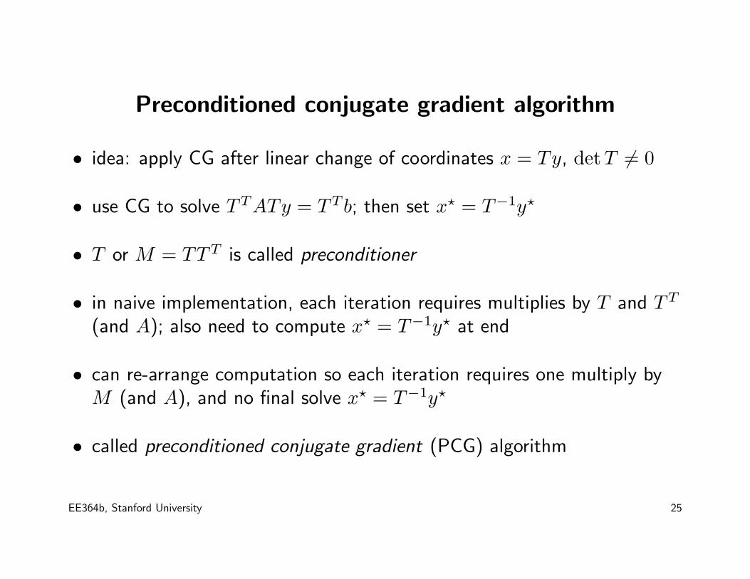
Preconditioned conjugate gradient algorithm

• idea: apply CG after linear change of coordinates x = Ty, detT 6= 0

• use CG to solve TTATy = TT b; then set x⋆ = T−1y⋆

• T or M = TTT is called preconditioner

• in naive implementation, each iteration requires multiplies by T and TT

(and A); also need to compute x⋆ = T−1y⋆ at end

• can re-arrange computation so each iteration requires one multiply byM (and A), and no final solve x⋆ = T−1y⋆

• called preconditioned conjugate gradient (PCG) algorithm


Choice of preconditioner

• if spectrum of TTAT (which is the same as the spectrum of MA) isclustered, PCG converges fast

• extreme case: M = A−1

• trade-off between enhanced convergence, and extra cost ofmultiplication by M at each step

• goal is to find M that is cheap to multiply, and approximate inverse ofA (or at least has a more clustered spectrum than A)


Some generic preconditioners

• diagonal: M = diag(1/A11, . . . , 1/Ann)

• incomplete/approximate Cholesky factorization: use M = A−1, whereA = LLT is an approximation of A with cheap Cholesky factorization

– compute Cholesky factorization of A, A = LLT

– at each iteration, compute Mz = L−T L−1z via forward/backwardsubstitution

• examples

– A is central k-wide band of A– L obtained by sparse Cholesky factorization of A, ignoring small

elements in A, or refusing to create excessive fill-in


Preconditioned conjugate gradient

(with preconditioner M ≈ A−1 (hopefully))

x := 0, r := b−Ax0, p := r z := Mr, ρ1 := rTz

for k = 1, . . . , Nmax

quit if√ρk ≤ ǫ‖b‖2 or ‖r‖ ≤ ǫ‖b‖2

w := Apα := ρk

wTp

x := x+ αpr := r − αwz := Mrρk+1 := zTrp := z +

ρk+1ρk

p


Larger example

residual convergence with and without diagonal preconditioning

0 10 20 30 40 50 6010

−8

10−6

10−4

10−2

100

102

104

k

η k


CG summary

• in theory (with exact arithmetic) converges to solution in n steps

– the bad news: due to numerical round-off errors, can take more thann steps (or fail to converge)

– the good news: with luck (i.e., good spectrum of A), can get goodapproximate solution in ≪ n steps

• each step requires z → Az multiplication

– can exploit a variety of structure in A– in many cases, never form or store the matrix A

• compared to direct (factor-solve) methods, CG is less reliable, datadependent; often requires good (problem-dependent) preconditioner

• but, when it works, can solve extremely large systems


Conjugate Gradient Method - Stanford University• incomplete/approximate Cholesky factorization:...

Documents

Transcript of Conjugate Gradient Method - Stanford University• incomplete/approximate Cholesky factorization:...