Confounding and Interaction: Part III Methods to reduce confounding –during study design:...

Confounding and Interaction: Part III• Methods to reduce confounding

– during study design:• Randomization• Restriction• Matching• Instrumental variables

– during study analysis:• Stratified analysis

– Forming “Adjusted” Summary Estimates– Concept of weighted average

» Woolf’s Method» Mantel-Haenszel Method

• Handling more than one confounder– Minimal sufficient adjustment set (MSAS)

• Managing uncertainty in your DAGs– Role of an analysis plan

• If time:– Residual confounding; importance of overlap; quantitative

bias analysis

• Limitations of stratification– Motivation for multivariable regression

• Limitations of conventional conditioning approaches– Motivation for other “non-conditioning” techniques

Effect-Measure Modification

DelayedNot

DelayedSmoking 15 61No Smoking 47 528

Stratified

Delayed Not DelayedSmoking 26 133No Smoking 64 601

Crude

No Caffeine Use

Heavy Caffeine Use

RR crude = 1.7

RRno caffeine use = 2.4

DelayedNot

DelayedSmoking 11 72No Smoking 17 73

RRcaffeine use = 0.7

. cs delayed smoking, by(caffeine) caffeine | RR [95% Conf. Interval] M-H Weight-----------------+------------------------------------------------- no caffeine | 2.414614 1.42165 4.10112 5.486943 heavy caffeine | .70163 .3493615 1.409099 8.156069 -----------------+------------------------------------------------- Crude | 1.699096 1.114485 2.590369 M-H combined | 1.390557 .9246598 2.091201-----------------+-------------------------------------------------Test of homogeneity (M-H) chi2(1) = 7.866 Pr>chi2 = 0.0050

Report interaction; managing confounding by summarizing the 2 stratum-specific estimates into 1 number not relevant (but confounding is managed)

Association Between Smoking and Delayed Conception by Amount of Caffeine Use

Caffeine Use Risk Ratio* 95% CI None 2.4** 1.4 to 4.1 Heavy 0.7** 0.35 to 1.4

* compares smokers to non-smokers (reference) ** test of homogeneity, p = 0.005

Report vs Ignore Effect-Measure Modification?Some Guidelines

Risk Ratios for a Given Exposure and Disease

Potential Effect Modifier Present Absent

P value for heterogeneity

Report or Ignore

Interaction

2.3 2.6 0.45 Ignore

2.3 2.6 0.001 Ignore

2.0 20.0 0.001 Report

2.0 20.0 0.10 Report

2.0 20.0 0.40 Ignore

3.0 4.5 0.30 Ignore

3.0 4.5 0.001 +/-

0.5 3.0 0.001 Report

0.5 3.0 0.15 +/-

Is an art form: requires consideration of clinical, statistical and practical considerations

P value threshold for reporting might be higher than other contexts, but interpretation is no different

Does AZT after needlesticks prevent HIV?

HIVNo

HIVAZT 8 40No AZT 16 28

24 68 92

Minor Severity

Major Severity

Crude

Stratified

HIV No HIVAZT 8 131No AZT 19 189

27 320 347

HIVNo


3 252 255

ORcrude = 0.61

OR = 0.0 OR = 0.35

. cc HIV AZTuse,by(severity)

severity | OR [95% Conf. Interval] M-H Weight-----------------+------------------------------------------------- minor | 0 0 2.302373 1.070588 major | .35 .1344565 .9144599 6.956522-----------------+-------------------------------------------------

Test of homogeneity (B-D) chi2(1) = 0.60 Pr>chi2 = 0.4400

Does AZT after needlesticks prevent HIV?

Report or ignore interaction?

. cc HIV AZTuse,by(severity)

severity | OR [95% Conf. Interval] M-H Weight-----------------+------------------------------------------------- minor | 0 0 2.302373 1.070588 major | .35 .1344565 .9144599 6.956522-----------------+-------------------------------------------------

Test of homogeneity (B-D) chi2(1) = 0.60 Pr>chi2 = 0.4400

Repor

t Int

erac

tion

- A

Need

mor

e inf

orm

ation

- C

Igno

re In

tera

ction

- B

What Next?

Minor Severity

Major Severity

Crude

Stratified


27 320 347

HIVNo


3 252 255

ORcrude = 0.61

OR = 0.0

HIVNo


24 68 92

OR = 0.35

How would you summarize these strata into one number?

Assuming Interaction is not Present, Form a Summary of the Unconfounded

Stratum-Specific Estimates

• Construct a weighted average– Assign weights to the individual strata– Summary Adjusted Estimate = Weighted

Average of the stratum-specific estimates

– a simple mean is a weighted average where the weights are equal to 1

– which weights to use depends on type of effect estimate desired (OR, RR, RD), characteristics of the data, and goal of research

– e.g., • Woolf’s method• Mantel-Haenszel method• Standardization (see text)

– Discussed earlier for age adjustment

ii

ii

w

istratuminestimateeffectw )] ([

5)1)(4(

)8(1)6(1)4(1)2(1mean simple

Forming a Summary Adjusted Estimate for Stratified Data

Minor Severity

Major Severity

Crude

Stratified


27 320 347

HIVNo


3 252 255

ORcrude = 0.61

OR = 0.0

HIVNo


24 68 92

OR = 0.35How would you weight these strata?

By sam

ple si

ze -

A

By inv

erse

of v

arian

ce -

E

By deg

ree

of b

alanc

e am

ong

case

s/

cont

rols

- C

By num

ber o

f cas

es -

B

Evenly

- D

Summary Estimators: Woolf’s Method

• aka Directly pooled or precision estimator

• Woolf’s estimate for adjusted odds ratio

– where wi

– wi is the inverse of the variance of the stratum-specific log(odds ratio)

idicibia1111

1

i

i

i

ii

Woolfw

w )]OR (log[

OR log

)(OR logOR WoolfWoolf e

Disease No DiseaseExposed ai bi

Unexposed ci di

Calculating a Summary Effect Using the Woolf Estimator

• e.g., AZT use, severity of needlestick, and HIV

Minor Severity

Major Severity

Crude

Stratified


27 320

HIVNo


3 252 255

ORcrude =0.61

OR = 0.0

HIVNo


24 68 92

OR = 0.35

281

161

401

81

1

1611

31

911

01

1

)]0.35 log(

281

161

401

81

1[)]0 log(

1611

31

911

01

1[

WoolfOR log

Problem: cannot take log of 0; cannot divide by zero

Summary Adjusted Estimator: Woolf’s Method

• Conceptually straightforward

• Best when:– number of strata is small– sample size within each stratum is large

• Cannot be calculated when any cell in any stratum is zero because log(0) is undefined– “1/2” cell corrections have been suggested but are

subject to bias

• Formulae for Woolf’s summary estimates for other measures (e.g., risk ratio, RD) available in texts and software documentation

• Rarely used in practice but most clearly illustrates weighting

Summary Adjusted Estimators: Mantel-Haenszel

• Mantel-Haenszel estimate for odds ratios

– ORMH =

– wi =

– wi is inverse of the variance of the stratum-specific odds ratio under the null hypothesis (OR =1)

i

ii

N

cb

i

ii

i

ii

Ncb

Nda

i

ii

i

i

i

i

i

ii

Ncb

dbca

Ncb

*

Disease No DiseaseExposed ai bi

Unexposed ci di

ai+ bi + ci + di = Ni

Summary Adjusted Estimator: Mantel-Haenszel

• Relatively resistant to the effects of large numbers of strata with few observations

• Resistant to cells with a value of “0”

• Computationally easy

• Bottomline:– Most commonly available technique in

commercial software

Calculating a Summary Adjusted Effect Using the Mantel-Haenszel Estimator

• ORMH =

• ORMH =

Minor Severity

Major Severity

Crude

Stratified


27 320

HIVNo


3 252 255

ORcrude =0.61

OR = 0.0

HIVNo


24 68 92

OR = 0.35

i

ii

ii

ii

i

ii

N

cbcb

da

N

cb*

i

ii

i

ii

Ncb

Nda

30.0

921640

255391

92288

2551610

Calculating a Summary Effect in Stata

• To stratify by a third variable:

– cs varcase varexposed, by(varthird variable)

– cc varcase varexposed, by(varthird variable)

• Default summary estimator is Mantel-Haenszel

– “ , pool” will also produce Woolf’s method

• To stratify by several variables:– mhodds varcase varexposed varsadjust, by(var_liststratify)

– Problem set this week

epitab command - Tables for epidemiologists

A good place to learn epidemiology

Calculating a Summary Effect Using the Mantel-Haenszel Estimator

• e.g., AZT use, severity of needlestick, and HIV

• . cc HIV AZTuse,by(severity) pool• severity | OR [95% Conf. Interval] M-H Weight• -----------------+-------------------------------------------------• minor | 0 0 2.302373 1.070588 • major | .35 .1344565 .9144599 6.956522 • -----------------+-------------------------------------------------• Crude | .6074729 .2638181 1.401432 • Pooled (direct) | . . .• M-H combined | .30332 .1158571 .7941072 • -----------------+-------------------------------------------------• Test of homogeneity (B-D) chi2(1) = 0.60 Pr>chi2 = 0.4400• Test that combined OR = 1:• Mantel-Haenszel chi2(1) = 6.06• Pr>chi2 = 0.0138

Minor Severity

Major Severity

Crude

Stratified


27 320

HIVNo


3 252 255

ORcrude =0.61

OR = 0.0

HIVNo


24 68 92

OR = 0.35

After the Point Estimate: Confidence Interval Estimation and

Hypothesis Testing for the Mantel-Haenszel Estimator

• e.g. AZT use, severity of needlestick, and HIV

• . cc HIV AZTuse,by(severity) pool• severity | OR [95% Conf. Interval] M-H Weight• -----------------+-------------------------------------------------• minor | 0 0 2.302373 1.070588 • major | .35 .1344565 .9144599 6.956522 • -----------------+-------------------------------------------------• Crude | .6074729 .2638181 1.401432 • Pooled (direct) | . . .

M-H combined | .30332 .1158571 .7941072

• -----------------+-------------------------------------------------• Test of homogeneity (B-D) chi2(1) = 0.60 Pr>chi2 = 0.4400

• Test that combined OR = 1:• Mantel-Haenszel chi2(1) = 6.06• Pr>chi2 = 0.0138

• ?

After Confounding is Managed: Confidence Interval Estimation and Hypothesis Testing

for the Mantel-Haenszel Estimator

• e.g. AZT use, severity of needlestick, and HIV

• . cc HIV AZTuse,by(severity) pool• severity | OR [95% Conf. Interval] M-H Weight• -----------------+-------------------------------------------------• minor | 0 0 2.302373 1.070588 • major | .35 .1344565 .9144599 6.956522 • -----------------+-------------------------------------------------• Crude | .6074729 .2638181 1.401432 • Pooled (direct) | . . .

M-H combined | .30332 .1158571 .7941072

• -----------------+-------------------------------------------------• Test of homogeneity (B-D) chi2(1) = 0.60 Pr>chi2 = 0.4400

• Test that combined OR = 1:• Mantel-Haenszel chi2(1) = 6.06• Pr>chi2 = 0.0138

• What does the p value = 0.0138 mean?

1.38

% p

roba

bility

that

the

adjus

ted

OR = 0

.30

is du

e to

chan

ce -

A

If th

ere

truly

is no

ass

ociat

ion b

etwee

n

azt a

nd H

IV a

cquis

ition

afte

r adju

stmen

t

for s

ever

ity o

f exp

osur

e, th

ere

is a

1.38

%

prob

abilit

y of o

btain

ing a

n OR o

f 0.3

0 or

mor

e ex

trem

e by

chan

ce a

lone.

- C

1.38

% p

roba

bility

that

the

diffe

renc

e

betw

een

crud

e an

d ad

juste

d OR is

due

to ch

ance

- B

Some

bette

r ans

wer -

D

Terminology

• “Use of AZT is associated with decreased odds of HIV acquisition, independent of needlestick severity”

• “Use of AZT is associated with decreased odds of HIV acquisition, adjusted for needlestick severity”

• “Use of AZT is associated with decreased odds of HIV acquisition, controlling for needlestick severity”

• “Use of AZT is associated with decreased odds of HIV acquisition, conditioned on needlestick severity”

“Independent of”

• “Use of AZT is associated with decreased odds of HIV acquisition, independent of needlestick severity”

• “independent of” simply refers to adjustment/control for specific factors– Does not refer to whether or not adjusted

estimate is different from crude

– Just means that adjustment has been performed (e.g., via stratification)

How about this?

• “Use of AZT is causally related to reduced HIV acquisition.”

• Formally, our analyses produce statistical associations, which could result from:– Causal relationship (Truth)

Or bias due to:– Selection bias– Measurement bias– Confounding bias

Or– Reverse causality (but not here since

we know AZT use came first)

Or– Chance

• Single observational study rarely proves causality

• Data themselves do not establish causality

- Scientists do, by consensus, by excluding the other 5 explanations

Mantel-Haenszel Confidence Interval and Hypothesis Testing

stratumeach in cell a

for the valueexpected theis E

)1(

5.0

eCI %95

;;;

)(2

)(

))((2

)(

)(2

)(

OR) (logSE

i

12

2121

2

1 121

)MH

OR SE(log x (1.96 MH

OR log

1

2

1

1 1

1

1

2

1

where

NN

mmnn

Ea

N

cbw

N

daR

N

cbQ

N

daP

where

w

wQ

wR

RQwP

R

RP

k

i ii

iiii

k

i

k

iii

i

iii

i

iii

i

iii

i

iii

k

ii

k

iii

k

i

k

iii

k

iiiii

k

ii

k

iii

Disease No DiseaseExposed ai bi m1i

Unexposed ci di m2i

n1i n2i Ni

Mantel-Haenszel Techniques

• Mantel-Haenszel estimators

• Mantel-Haenszel chi-square statistic

• Mantel’s test for trend (dose-response)

More than One ConfounderMore than One Confounder

RQ: Does Chlamydia pneumoniae infection cause coronary artery disease (CAD)?

RQ: Does Chlamydia pneumoniae infection cause coronary artery disease (CAD)?

AgeAge

??

Chlamydia pneumoniae

infection

Chlamydia pneumoniae

infection

CADCAD

SmokingSmoking

Stratifying by Multiple Confounders

Confounders: Age and Smoking

• To control for multiple confounders simultaneously, must construct mutually exclusive and exhaustive strata:

<40 yo 40-60 yo >60 yo

Smokers Non-smokers

Because Confounders Operate Together in Nature, Joint Stratification is Needed

Crude

Stratified

<40 smokers

>60 non-smokers40-60 non-smokers

CAD NoCAD

Chlamydia

NoChlamydia

<40 non-smokers

40-60 smokers >60 smokers

CAD No CADChlamydiaNo chlamydia

CAD NoCAD

Chlamydia

NoChlamydia

CAD NoCAD

Chlamydia

NoChlamydia

CAD NoCAD

Chlamydia

NoChlamydia

CAD NoCAD

Chlamydia

NoChlamydia

CAD NoCAD

Chlamydia

NoChlamydia

Next steps: Assess for interaction… summarize….

Murray et al. Population Health Metrics 2003

WHO Causal Model of Coronary Heart Disease

Minimal Sufficient Adjustment Sets(MSAS)

• Minimal set of variables, which if controlled for, will allow for estimation of causal effect of E on D

• i.e., the minimal set of factors you need to control for that will:– keep all causal paths open– and– close all non-causal paths

• Remember, the general statistical term for “controlled for” is “condition”– means to hold constant– techniques include: restriction, matching,

stratification, or mathematical regression

• For any DAG, there may be several minimal sufficient adjustment sets (MSAS’s).

• Real life DAGs make it very difficult for the human eye to manually determine the MSAS’s

• DAGitty.net makes it simple

This is the major innovation of this software

Why might we decide to adjust for one MSAS over another?

• Not all variables are created equal– i.e., not all variables are equally easy to control for

• Some variables:– Have lots of missing data

– Are poorly measured • Either reproducibility or validiity

– Difficult to quantity• e.g., injection drug use, or hypertension

– Difficult to specify• e.g., continuous variables

– Expensive to measure

– Involve ethical issues if measured• e.g., illegal behavior (drug use; commercial sex)

• Advice– Choose MSAS which has variables that are most

feasible, reproducible, accurate, and manageable

Need h in all scenarios

If k is a problem to measure, go for {a, h, i}

The IdealYou are confident about the DAG

• Find all the MSASs

• Choose the most practical MSAS

• Adjust for the chosen MSAS– Via restriction, matching, stratification, or

regression

• Report the final adjusted measure of association

• Why not just take the most conservative route and adjust for everything that is conceivable?

The Reality

AA

??EE DD

BB

??

??

You are often NOT confident about the DAG

Lung CaNo

Lung CASmoking 810 270No Smoking 10 70

Lung CaNo

Lung CASmoking 90 30No Smoking 90 630

OR crude = 21.0

(95% CI: 16.4 - 26.9)

OR no matches = 21.0

Lung Ca No Lung CaSmoking 900 300No Smoking 100 700

Stratified

Crude

Matches Absent

Matches Present

ORmatches = 21.0

OR adj MH = 21.0 (95% CI: 14.2 - 31.1)

Which will you report as your final answer?

Crude

- A

Need

mor

e inf

orm

ation

- C

Adjuste

d - B

No indication from the DAG that Matches must be controlled for

??SmokingSmoking

Lung CancerLung

Cancer

MatchesMatches

Effect of Adjustment on Precision (Variance)

• Adjustment (e.g., stratification) is not all good

• Adjustment can increase or decrease standard errors (and CI’s) depending upon:– Nature of outcome (interval scale vs. binary)– Measure of association desired– Method of adjustment (Woolf vs M-H vs MLE)– Strength of association between potential

confounding factor and exposure/disease

• Difficult to predict effect on precision

• Good news: adjustment for strong confounders removes bias and often improves precision

• Bad news: adjustment for less-than-strong confounders can often (but not always) worsen precision

Spermicides, maternal age & Down Syndrome

Down No Down

Spermici use 3 104 No spermic. 9 1059 1175

Down No Down

Spermic. use 1 5 No spermic. 3 86 95

Down No Down Spermicide use 4 109 No spermicide use 12 1145

Age < 35 Age > 35

Crude

Stratified

OR = 3.4 OR = 5.7

OR = 3.5

. cc downs spermici , by(matage) pool matage | OR [95% Conf. Interval] M-H Weight -----------------+------------------------------------------------- < 35 | 3.394231 .9800358 11.80389 .7965957 >= 35 | 5.733333 0 50.8076 .1578947 -----------------+------------------------------------------------- Crude | 3.501529 1.171223 10.49699 Pooled (direct) | 3.824166 1.196437 12.22316 M-H combined | 3.781172 1.18734 12.04142 -----------------+------------------------------------------------- Test for heterogeneity (direct) chi2(1) = 0.137 Pr>chi2 = 0.7109 Test for heterogeneity (M-H) chi2(1) = 0.138 Pr>chi2 = 0.7105 Test that combined OR = 1: Mantel-Haenszel chi2(1) = 5.81 Pr>chi2 = 0.0159

Which answer should you report as “final”?

Crude

- A

Need

mor

e inf

orm

ation

- C

Adjuste

d - B

What if you don’t know if the red edge exists? (i.e., existing literature is inconclusive)

??

Spermicide use

Spermicide use

Down Syndrome

Down Syndrome

AgeAge

??

Whether or not to accept the “adjusted” summary estimate instead

of the crude?• No one correct answer

– “Bias-variance tradeoff”

• Scientifically rigorous approach is to:– Create the DAG and identify potential confounders– Prior to adjustment, classify the potential

confounders as either being:• “A” List: Those factors for which you will accept

the adjusted result no matter how small the difference from the crude.

– Factors strongly believed to be confounders

• “B” List: Those factors for which you will accept the adjusted result only if it meaningfully differs from the crude (with some pre-specified difference, e.g., 5 to 10%).

– Factors you are less sure about– “Change-in-estimate” approach

• For some analyses, may have no factors on B list. For other analyses, some factors on B list.

• Always putting all factors on A list may seem “conservative”, but not necessarily the right thing to do in light of penalty of statistical imprecision

Bias control paramount

Need for tradeoffs

Spermicide use

Spermicide use

AgeAge

??

Down Syndrome

Down Syndrome??

Adjusting for Age?Adjusting for Age?

Age is on “A” List

Adjust for Age; Accept OR = 3.8 as

final estimate

Age is on “A” List

Adjust for Age; Accept OR = 3.8 as

final estimate

Age is on “B” List

Adjust for Age only if

exceeds pre-

specified change-in- estimate threshold (e.g., 10%)

Age is on “B” List

Adjust for Age only if

exceeds pre-

specified change-in- estimate threshold (e.g., 10%)

AgeAge

??Down

Syndrome

Down Syndrome

Spermicide use

Spermicide use

Whether age is on “A” or “B” list should be pre-specified in your analysis plan

Choosing the crude or adjusted estimate?

• Assume no interaction• Factors on B list have 10% change-in-estimate

rule in place

Risk Ratios

List

Crude Third Factor Present

Third Factor Absent

Adjusted Choose?

B 4.1 1.9 2.1 2.0 Adjusted

A 4.0 1.2 1.0 1.1 Adjusted

B 0.2 0.7 0.9 0.8 Adjusted

A 4.0 3.8 4.2 4.1 Adjusted

B 4.0 4.1 4.7 4.3 Crude

“Change in Estimate” Approach– A Historical Perspective

• Historically, confounding was defined by whether the adjusted estimate differed from the crude– “if there is a change after adjustment, there has to

be confounding present”

• i.e., in the past, the data defined confounding– “data-based definition of confounding”

• Today, philosophy is very different– We primarily don’t use data from the current

study to define presence or absence confounding or what to control for

• e.g., if we adjust for something and it changes the estimate, we don’t accept this as confounding unless there was some a priori belief (e.g., gum chewing in melonoma)

– Exception: if the prior literature is uncertain about a part of a DAG, it is reasonable to use data from current study to weigh in on the decision to adjust

• This is the “change in estimate” approach

No Role for Statistical Testing for Confounding

• Testing for statistically significant differences between crude and adjusted measures is inappropriate

• e.g., examining an association for which a factor is a known confounder (say age in the association between hypertension and CAD)

– if the study has a small sample size, even large differences between crude and adjusted measures may not be statistically different

• yet, we know confounding is present• therefore, the difference between crude and

adjusted measures cannot be ignored as merely chance.

• bias must be prevented and hence adjusted estimate is preferred

• we must live with whatever effects we see after adjustment for a factor for which there is a strong a priori belief about confounding

• If study has large sample size, even small differences between crude and adjusted will be significant. Would you accept all of these adjustments to be necessary even if no a priori evidence of confounding?

The IdealYou are confident about the DAG

• Find all the MSASs

• Choose the most practical MSAS

• Adjust for the chosen MSAS– Via restriction, matching, stratification, or

regression

• Report the final adjusted measure of association

• Why not just take the most conservative route and adjust for everything that is conceivable?

The RealityYou are often NOT confident about the DAG

• Bias (if inadvertent adjustment on a collider)

• Problems with this approach:• Precision (increase variance)

Controlling for M gives a desirable resultControlling for M gives a desirable result

Direction of an Edge Can Make a Big Difference

U1U1 U2

U2

??DDEE

MM

Controlling for M induces collider biasControlling for M induces collider bias

EE??

DD

U1U1 U2

U2

MM

Solution: If crude & adjusted estimates differ by > 5% to 10%, report both analyses and discuss the influence of this unknown direction

• Pre-specify % in your analysis plan

What About Multiple Areas of Uncertainty?

??

?

How to handle multiple areas of uncertainty in complex DAGs?

• No one best approach – Frontier of methodologic research

Common MSAS’s present across the DAGs

Adjust for the common MSAS

Our advice features transparency

Does any uncertainty involve colliders?

No Yes

Draw the different possible DAGs & find the MSAS’s

No common MSAS’s across the DAGs

Determine adjusted estimate that includes all of the uncertain relationships (all of the B list variables). Consider this “maximally adjusted”.

One by one, recalculate adjusted estimate without one of the B list variables. Drop the B list variable if its exclusion results in an estimate no more than some threshold (e.g., 5% to 10%) away from maximally adjusted estimate. Stop when no more B list variables can be dropped.

Next slide Done

How to handle multiple areas of uncertainty in complex DAGs?

Common MSAS’s present across the DAGs

Adjust for the common MSAS

Does any uncertainty involve colliders?

No Yes

Additional approaches in BIOSTAT 208 and 209

Draw the different possible DAGs & find the MSAS’s

No common MSASs across the DAGs

Must reduce potential DAGs to some reasonable number

Done

Determine adjusted estimate for the different DAGs

Report adjusted estimates for the different DAGs

Prior slide

Discuss which uncertain relationships are most influential & highlight them for future research

They are all close (within 5% to 10%)

They are NOT close

Done

An Analysis Plan• How to select variables to control for (“final model”) is

one of the least standardized processes

• Available methods often arbitrary and can give different answers for the “final estimate”– Invites fishing for desired answers

• Solution: Analysis plan

• Written before the data are analyzed

• Content– Detailed description of the techniques to be used to

analyze data, step by step

– Forms the basis of “Statistical Analysis” section in manuscripts

– Parameters/rules/logic to guide key decisions:

• which variables will be assessed for interaction and for adjustment?

• what p value and magnitude of heterogeneity will be used to guide reporting of interaction?

• what is a meaningful change-in-estimate threshold between two estimates (e.g., 5% or 10%) to determine variable selection and model reporting?

• Utility: A plan helps to keep the analysis:– Focused

– Transparent

– Reproducible

– Honest (avoids p value shopping)

Transparency of Analytic Plans

• Poor Quality of Reporting Confounding Bias in Observational Studies: A Systematic Review. Groenwold et al. Ann Epid 2008

• Review of 174 observational studies, 2004 - 2007

Characteristic No. (%) Articles in Compliance

Reporting of why potential confounding factors are selected for analysis

18 (10.3%)

Reporting of reasons why factors were included in final adjusted analysis

88 (50.6%)

Stratification to Manage Confounding

• Advantages– straightforward to implement and comprehend– many reviewers phobic of regression– easy way to evaluate interaction

• Limitations– Requires continuous variables to be discretized

• loses information; possibly results in “residual confounding”

• discretizing often brings less precision

– Deteriorates with multiple confounders• e.g., suppose 4 confounders with 3 levels

– 3x3x3x3=81 strata needed– unless huge sample, many cells have “0”’s and

strata have undefined effect measures

– Conventional Conditioning Solution:• Mathematical modeling (aka, multivariable

regression)– e.g.,

» linear regression» logistic regression» proportional hazards regression

See BIOSTAT 208 & 209

Limitation of Conventional Regression (as well as Stratification)

• Scenario: Time-varying exposures in the presence of time-varying confounders which are also mediators of relevant causal paths– e.g., Cohort study of effect of antiretroviral therapy (ART) on AIDS incidence

Simultaneous desire to control for CD4 to manage confounding and but NOT to control because it is a mediator of one of the relevant direct causal paths

AIDSAIDSART time1 ART time1

CD4 time1CD4 time1

??ART time 2 ART time 2

CD4 time2CD4 time2

??

Time-varying exposures in the presence of time-varying confounders

which are also mediators of relevant causal paths

“Weighted” refers to inverse probability weighting (marginal structural models)

Cole et al, AJE 2003

Limitation of Conventional Regression (as well as Stratification)

• Scenario: Determining a direct effect

– e.g., Estimating direct effect of E on D apart from effect on I (“mediation analysis”)

Simultaneous desire to control for I to get direct effect of E and but NOT to control because I is a collider

Other non-conditioning methods needed

DDE E

Unmeasured Confounder

Unmeasured Confounder

??

II

Non-Conditioning Approaches to Manage Confounding

• Conditioning approaches:– e.g., restriction, matching, stratification, regression– Compare exposed to unexposed at fixed levels of

the confounders

• In contrast, non-conditioning approaches:– first balance exposed and unexposed groups for

the confounder • then compare exposed to unexposed• This is what randomization does, but non-

conditioning techniques for observational analysis are much more complicated!

– Several different techniques:• G-estimation • Structural nested models• Marginal structural models (e.g., inverse

probability weighting)– currently, most popular

• (and others)• See BIOSTAT 215

• Goal for you• Recognize when the techniques are needed

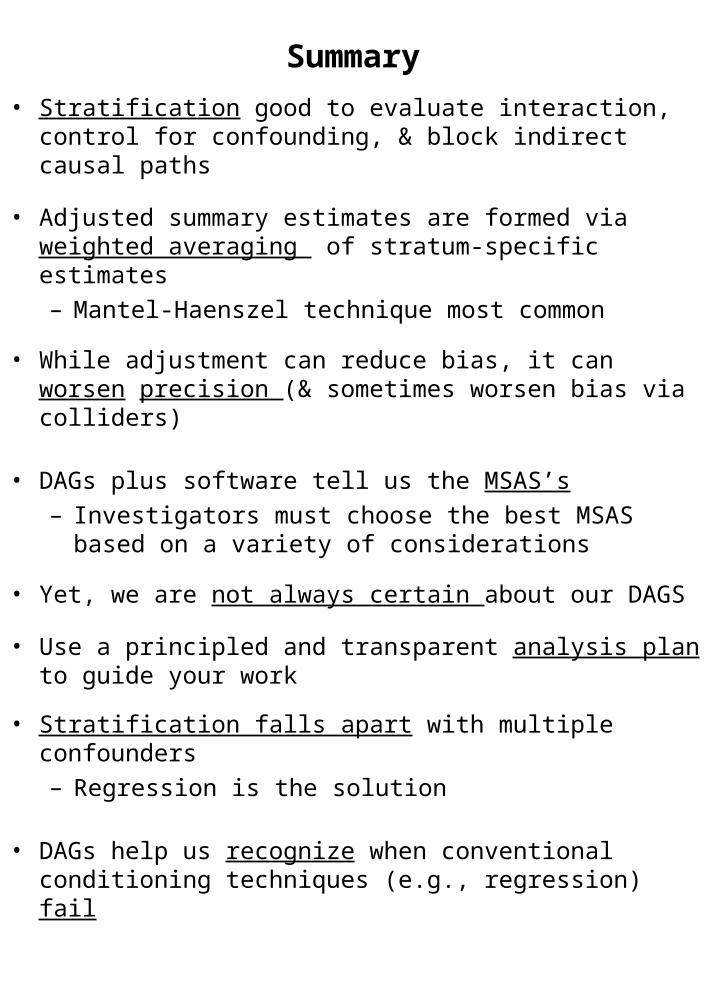
Summary

• Stratification good to evaluate interaction, control for confounding, & block indirect causal paths

• Adjusted summary estimates are formed via weighted averaging of stratum-specific estimates

– Mantel-Haenszel technique most common

• While adjustment can reduce bias, it can worsen precision (& sometimes worsen bias via colliders)

• DAGs plus software tell us the MSAS’s

– Investigators must choose the best MSAS based on a variety of considerations

• Yet, we are not always certain about our DAGS

• Use a principled and transparent analysis plan to guide your work

• Stratification falls apart with multiple confounders

– Regression is the solution

• DAGs help us recognize when conventional conditioning techniques (e.g., regression) fail

• Next Tuesday (Dec. 4, 2012) – 8:45 to 10:15: Journal Club

– 1:30 to 3:00 pm: Last Section• Web-based course evaluation• Bring laptop

– Distribute Final Exam (on website)• Exam due Dec. 11 in hands of Olivia

by 4 pm by email ([email protected]) or China Basin 5700

Extra Slides

Remember the Research Purpose When Performing Adjustment

• We have focused on adjustment for causal hypothesis testing of a single exposure variable

• However, there are other purposes why we adjust

– Evaluating multiple exposure variables

– Prediction of outcome by variables (even if non-causal)

• These other research purposes require different approaches to what variables to adjust for

Importance of Overlap of the Confounder

2. Matching provides a way to ensure overlap between comparator groups (e.g., cases/controls) in the distribution of confounders other than complex nominal variables

e.g., Case-control study of prostate cancer -- confounding by age– Cases will have many old individuals– Random sampling of controls, especially in

smaller studies, apt not to contain oldest individuals

– Matching age distribution of controls to age distribution of cases ensures complete overlap in age between cases and controls

casescontrols

Age

Age

From Last Week

Importance of Overlap of the Confounder

• Overlap is guaranteed in randomization, restriction, and matching

• But not guaranteed in stratification or regression

• In stratification, lack of overlap will result in unused strata and wasted data

• In regression, certain assumptions are made about the non-overlap zones (based on behavior of the data in overlap zones)– Typically without the investigator being aware– Can lead to bias

• Advice– Look for presence of overlap of confounder

distributions between comparator groups – Propensity scores are easiest approach

• Lack of overlap also called:– Positivity violation– Experimental treatment allocation (ETA)

violation

Residual Confounding (i.e. confounding still present after adjustment)

Four Mechanisms

1. Categorization of confounder too broad– e.g., Association between natural

menopause and prevalent CHD

Szklo and Nieto, 2007

Method of age adjustment OR 95% CI Crude 4.54 2.67-7.85 2 categories: 45-54, 55-64 3.35 1.60-6.01 4 categories: 45-49, 50-54, 55-59, and 60-64

3.04 1.37-6.11

Continuous variable 2.47 1.31-4.63

2. Misclassification of confounders – Can be differential or non-differential

with respect to exposure and disease

– If non-differential, will lead to adjusted estimates somewhere in between crude and true adjusted

– If differential, can lead to a variety of unpredictable directions of bias

Residual ConfoundingMechanisms – cont’d

3. Variable used for adjustment is imperfect proxy for true confounder

CRP levelCRP level

??

Periodontal disease

Periodontal disease

Inflammatory PredispositionInflammatory Predisposition

CADCAD

4. Unmeasured confounders

AgeAge

??E E DD

Unmeasured CUnmeasured C

Quantitative Analysis of Unmeasured Confounding

• Can back calculate to determine how a confounder would need to act in order to spuriously cause any apparent odds ratio. Example: observed OR= 2.0

Prevalence of “high” level of unmeasured confounder

Association between unmeasured confounder and disease (risk ratio)

Ass

ocia

tion

betw

een

unm

easu

red

conf

ound

er a

nd

expo

sure

(pr

eval

ence

rat

io)

A (low prevalence scenario) = 7 B (high prevalence scenario) = 3.4

Winkelstein et al., AJE 1984

Quantitative assessment of unmeasured confounders

• Exposure was deferral of anti-HIV therapy and outcome was death. Observed risk ratio was 1.94.

• “The contour plot shows that a confounding factor with a relative risk for death of 4.0 and an odds ratio for deferral of therapy of 4.0 after adjustment for all included variables would reduce the estimated relative risk for deferred therapy to approximately 1.30.”

Kitahata et al. NEJM 2009

Quantitative Bias Analysis

• Our discussion of selection, measurement, and confounding bias has been qualitative

• Frontier of epidemiologic methods is quantitative bias analysis– Selection bias: use estimates of selection

probabilities to back-calculate to truth

– Measurement bias: use estimates of misclassification to back-calculate to truth

– Confounding: How would results change in presence of certain confounding factors of a given strength of association with exposure and outcome?

Regression is ahead but don’t forget about the simple

techniques …..• “Because of the increased ease and availability of

computer software, the last few years have seen a flourishing of the use of multivariate analysis in the biomedical literature. These highly sophisticated mathematic models, however, rarely eliminate the need to examine carefully the raw data by means of scatter diagrams, simple n x k table, and stratified analyses.” Szklo and Nieto 2007

• “The widespread availability and user-friendly nature of computer software make the method accessible to some data analysts who may not have had adequate instruction in its appropriate applications. When they are misapplied, multivariate techniques have the potential to contribute to incorrect model development, misleading results, and inappropriate interpretation of the effect of hypothesized confounders.”

Friis and Sellers, 2009

Two Reasons to Adjust

1. Close a backdoor path generated by a non-collider which is a “common cause” (a confounder)

2. Close an indirect path which is a nuisance/ – estimating “direct effect” of E, apart from its effect

on X (e.g., poor diet)

Nightlights Nightlights

Child’s myopia

Child’s myopia

Parental myopia

Parental myopia

??

PovertyPoverty

MortalityMortality

Poor DietPoor Diet ??

Same 4 residual mechanisms also pertain to this reason for adjustment -- results in “incomplete adjustment for indirect causal pathways”

Confounding and Interaction: Part III Methods to reduce confounding –during study design:...

Documents

Transcript of Confounding and Interaction: Part III Methods to reduce confounding –during study design:...