Confounding and Interaction: Part II Methods to reduce confounding –during study design:...
47
Confounding and Interaction: Part II Methods to reduce confounding – during study design : » Randomization » Restriction » Matching – during study analysis: » Stratified analysis Interaction – What is it? How to detect it? – Additive vs. multiplicative interaction – Comparison with confounding – Statistical testing for interaction – Implementation in Stata
-
Upload
anthony-hunter -
Category
Documents
-
view
225 -
download
0
Transcript of Confounding and Interaction: Part II Methods to reduce confounding –during study design:...

Confounding and Interaction: Part II
Methods to reduce confounding
– during study design:
» Randomization
» Restriction
» Matching
– during study analysis:
» Stratified analysis
Interaction
– What is it? How to detect it?
– Additive vs. multiplicative interaction
– Comparison with confounding
– Statistical testing for interaction
– Implementation in Stata

Confounding
ConfounderConfounder
DD
ANOTHER PATHWAY TO
GET TO THE DISEASE
(a mixing of effects)
ANOTHER PATHWAY TO
GET TO THE DISEASE
(a mixing of effects)
RQ: Is E associated with D independent of C?
RQ: Is E associated with D independent of C?

Methods to Prevent or Manage Confounding
DD
DD
oror
By prohibiting at least one “arm” of the exposure- confounder - disease structure, confounding is precluded

Randomization to Reduce Confounding
Definition: random assignment of subjects to exposure (e.g., treatment) categories
All subjects Randomize
Distribution of any variable is theoretically the same in the exposed group as the unexposed
– Theoretically, can be no association between exposure and any other variable
One of the most important inventions of the 20th Century!
Exposed
(treatment)
Unexposed

Randomization to Reduce Confounding
DD
Explains the exulted role of randomization in clinical research
Randomization prevents confounding

Randomization to Reduce Confounding
All subjects Randomize
Of course, applicable only for intervention (experimental) studies
Special strength of randomization is its ability to control the effect of confounding variables about which the investigator is unaware
– Because distribution of any variable theoretically same across randomization groups
Does not, however, always eliminate confounding!
– By chance alone, there can be imbalance– Less of a problem in large studies– Techniques exist to ensure balance of certain
variables
Exposed
Unexposed
Restriction to Reduce Confounding
AKA Specification
Definition: Restrict enrollment to only those subjects who have a specific value/range of the confounding variable
– e.g., when age is confounder: include only subjects of same narrow age range
But what if we cannot randomize?
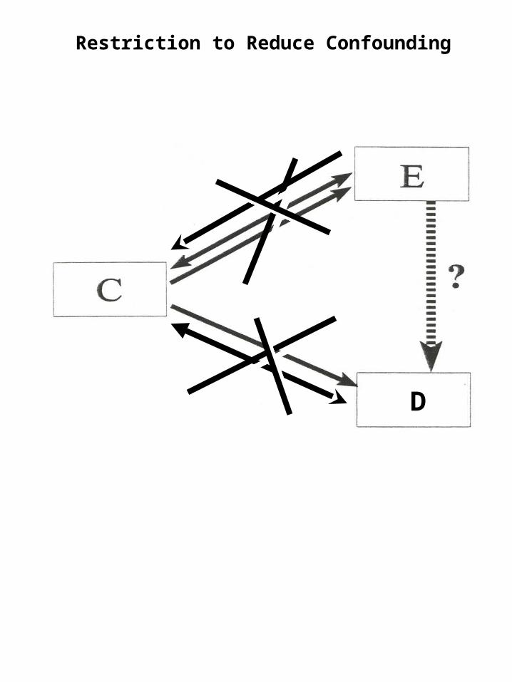
Restriction to Reduce Confounding
DD

Restriction to Prevent Confounding
Particularly useful when confounder is quantitative in scale but difficult to measure
e.g.
– Research question: Is there an association between sexual behavior and acquisition of HHV-8 infection?
– Issue: Is association confounded by injection drug use?
– Problem: degree of injection drug use is difficult to measure
– Solution: restrict to subjects with no injection drug use, thereby precluding the need to measure degree of injection use
– Cannon et. al NEJM 2001
» Restricted to persons denying injection drug use
Commercial sex No. % HHV-8-positive Odds Ratio
No 311 9.6 1.0 Yes 160 18.8 2.2 (1.3 to 3.7)

Restriction to Reduce Confounding
Advantages:
– conceptually straightforward
– handles difficult to quantitate variables
– can also be used in analysis phase
Disadvantages:
– may limit number of eligible subjects
– inefficient to screen subjects, then not enroll
– “residual confounding” may persist if restriction categories not sufficiently narrow (e.g. “20 to 30 years old” might be too broad)
– limits generalizability (but don’t worry too much about this)
– not possible to evaluate the relationship of interest at different levels of the restricted variable (i.e. cannot assess interaction)
Bottom Line
– not used as much as it should be

Matching to Reduce Confounding
A complex topic
Definition: only unexposed/non-case subjects are chosen who match those of the comparison group (either exposed or cases) in terms of the confounder in question
Mechanics depends upon study design:
– e.g. cohort study: unexposed subjects are “matched” to exposed subjects according to their values for the potential confounder.
» e.g. matching on race
One unexposedblack enrolled for each exposedblack
One unexposedasian enrolled for each exposedasian
– e.g. case-control study: non-diseased controls are “matched” to diseased cases
» e.g. matching on age
One controlage 50 enrolled for each caseage 50
One controlage 70 enrolled for each caseage 70

Matching to Reduce Confounding
DD
DD
oror
Cohort design
Case-control design
Also illustrates a disadvantage

Advantages of Matching
1. Useful in preventing confounding by factors which would be impossible to manage in design phase
– e.g. “neighborhood” is a nominal variable with multiple values (complex nominal variable)
– e.g. Case-control study of the effect of a second BCG vaccine in preventing TB (Int J Tub Lung Dis. 2006)
» Cases: newly diagnosed TB in Brazil
» Controls: persons without TB
» Exposure: receipt of a second BCG vaccine
» Potential confounder: neighborhood of residence; related to ambient TB incidence and practices regarding second BCG vaccine
» Relying upon random sampling of controls without attention to neighborhood may result in (especially in a small study) choosing no controls from some of the neighborhoods seen in the case group (i.e., cases and controls lack overlap)
Matching on neighborhood ensures overlap
» Even if all neighborhoods seen in the case group were represented in the control group, adjusting for neighborhood with “analysis phase” strategies is problematic

If you chose to stratify to manage confounding, the number of strata may be unwieldy
Crude
StratifiedMission
CastroPacific Heights
TB No TB
BCB
No BCG
Marina
Sunset Richmond
TB No TB
BCG No BCG
Matching avoids this
TB No TB
BCB
No BCG
TB No TB
BCB
No BCG
TB No TB
BCB
No BCG
TB No TB
BCB
No BCG
TB No TB
BCB
No BCG

Advantages of Matching
2. By ensuring a balanced number of cases and controls (in a case-control study) or exposed/unexposed (in a cohort study) within the various strata of the confounding variable, statistical precision is increased

Smoking, Matches, and Lung Cancer
Lung Ca No Lung CaMatches 820 340No Matches 180 660
Lung CaNo
Lung CAMatches 810 270No Matches 90 30
900 300
B. Controls matched on smoking
A. Random sample of controls
Crude
Non-SmokersSmokers
OR crude = 8.8
OR CF+ = ORsmokers = 1.0 OR CF- = ORnon-smokers = 1.0
ORadj= 1.0 (0.75 to 1.34)
Lung CaNo
Lung CAMatches 10 70No Matches 90 630
100 700
Stratified
Smokers Non-Smokers
OR CF+ = ORsmokers = 1.0 OR CF- = ORnon-smokers = 1.0
ORadj= 1.0 (0.69 to 1.45)
Lung CaNo
Lung CAMatches 810 810No Matches 90 90
900 900
Lung CaNo
Lung CAMatches 10 10No Matches 90 90
100 100
Little known benefit of matching: Improved precision
Disadvantages of Matching
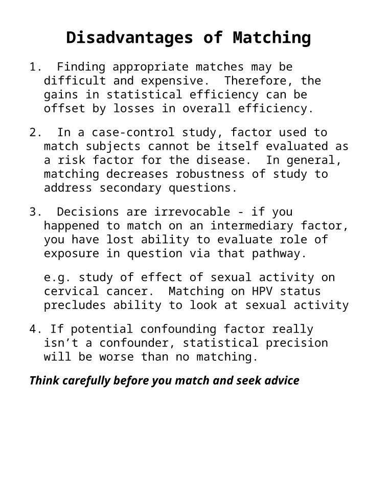
1. Finding appropriate matches may be difficult and expensive. Therefore, the gains in statistical efficiency can be offset by losses in overall efficiency.
2. In a case-control study, factor used to match subjects cannot be itself evaluated as a risk factor for the disease. In general, matching decreases robustness of study to address secondary questions.
3. Decisions are irrevocable - if you happened to match on an intermediary factor, you have lost ability to evaluate role of exposure in question via that pathway.
e.g. study of effect of sexual activity on cervical cancer. Matching on HPV status precludes ability to look at sexual activity
4. If potential confounding factor really isn’t a confounder, statistical precision will be worse than no matching.
Think carefully before you match and seek advice
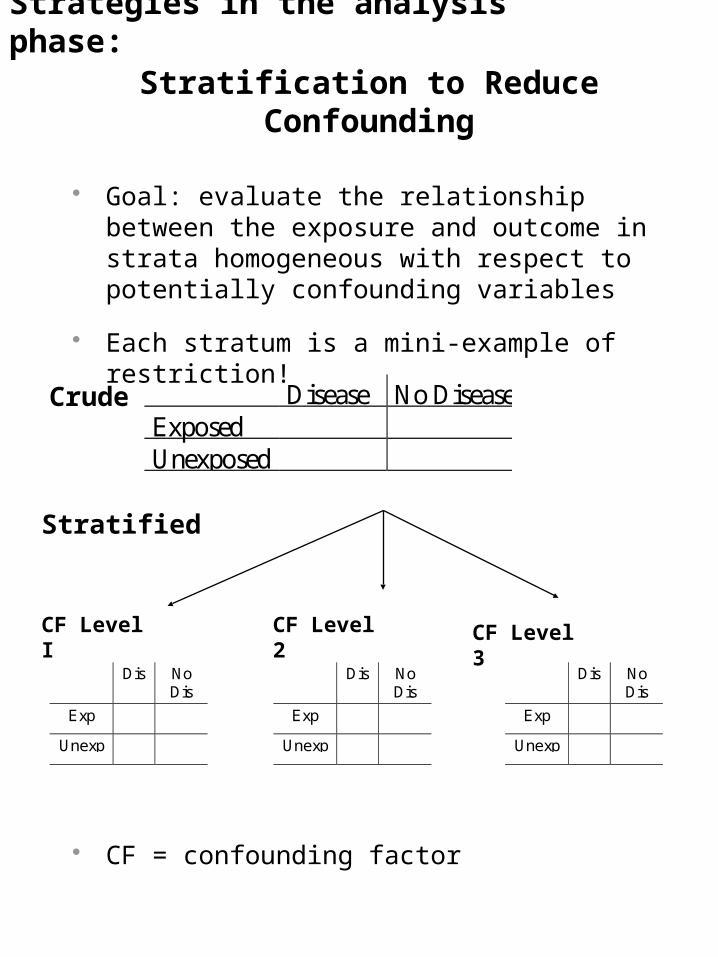
Stratification to Reduce Confounding
Goal: evaluate the relationship between the exposure and outcome in strata homogeneous with respect to potentially confounding variables
Each stratum is a mini-example of restriction!
CF = confounding factor
Disease No DiseaseExposedUnexposed
Crude
Dis NoDis
Exp
Unexp
Dis NoDis
Exp
Unexp
Dis NoDis
Exp
Unexp
Stratified
CF Level I CF Level 3CF Level 2
Strategies in the analysis phase:

Smoking, Matches, and Lung Cancer
Lung Ca No Lung CaMatches 820 340No Matches 180 660
Lung CaNo
Lung CAMatches 810 270No Matches 90 30
Stratified
Crude
Non-SmokersSmokersOR crude
OR CF+ = ORsmokers OR CF- = ORnon-smokers
ORcrude = 8.8
Each stratum in unconfounded with respect to smoking
ORsmokers = 1.0
ORnon-smoker = 1.0
Lung CaNo
Lung CAMatches 10 70No Matches 90 630
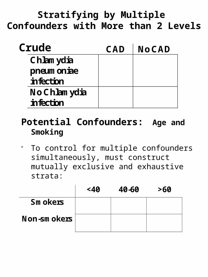
Stratifying by Multiple Confounders with More than 2 Levels
Potential Confounders: Age and Smoking
To control for multiple confounders simultaneously, must construct mutually exclusive and exhaustive strata:
<40 40-60 >60
Smokers Non-smokers
Crude CAD No CAD Chlamydia pneumoniae infection
No Chlamydia infection
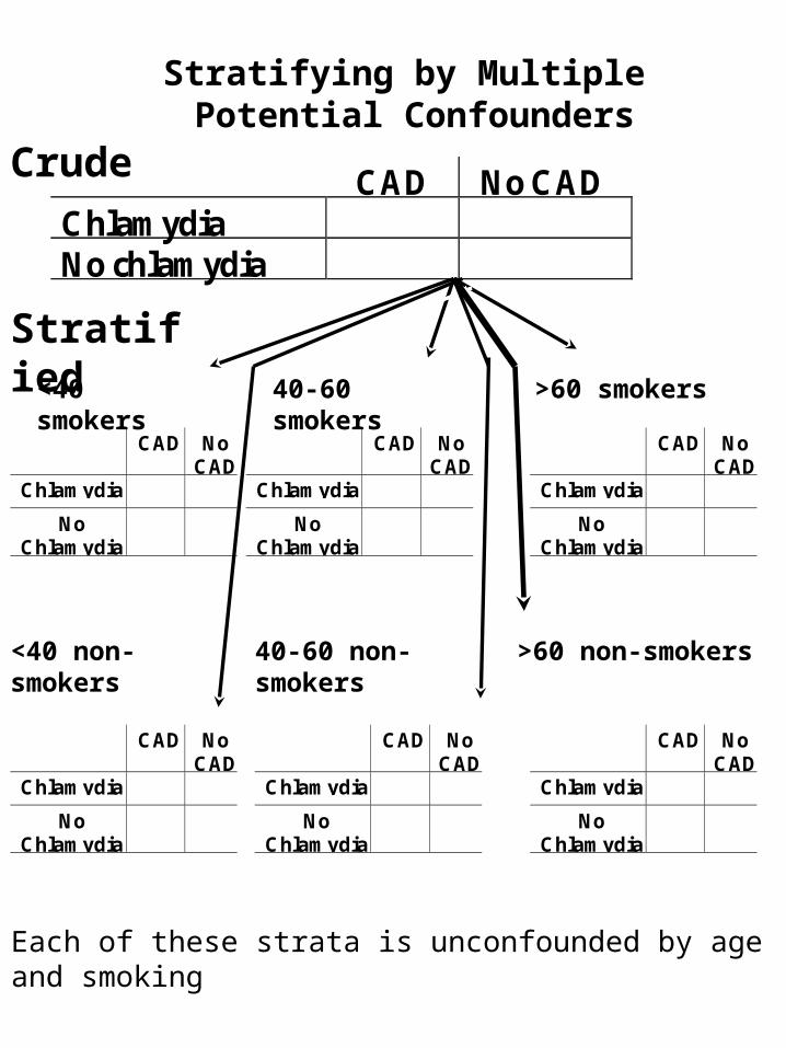
Stratifying by Multiple Potential Confounders
Crude
Stratified<40 smokers
>60 non-smokers40-60 non-smokers
CAD NoCAD
Chlamydia
NoChlamydia
<40 non-smokers
40-60 smokers >60 smokers
CAD No CADChlamydiaNo chlamydia
CAD NoCAD
Chlamydia
NoChlamydia
CAD NoCAD
Chlamydia
NoChlamydia
CAD NoCAD
Chlamydia
NoChlamydia
CAD NoCAD
Chlamydia
NoChlamydia
CAD NoCAD
Chlamydia
NoChlamydia
Each of these strata is unconfounded by age and smoking

Summary Estimate from the Stratified Analyses
After the stratum have been formed, what to do next?
Goal: Create a single unconfounded (“adjusted”) estimate for the relationship in question
– e.g., relationship between matches and lung cancer after adjustment (controlling) for smoking
Process: Summarize the unconfounded estimates from the two (or more) strata to form a single overall unconfounded “summary estimate”
– e.g., summarize the odds ratios from the smoking stratum and non-smoking stratum into one odds ratio

Smoking, Matches, and Lung Cancer
Lung Ca No Lung CaMatches 820 340No Matches 180 660
Lung CaNo
Lung CAMatches 810 270No Matches 90 30
Stratified
Crude
Non-SmokersSmokersOR crude
OR CF+ = ORsmokers OR CF- = ORnon-smokers
ORcrude = 8.8 (7.2, 10.9)
ORsmokers = 1.0 (0.6, 1.5)
ORnon-smoker = 1.0 (0.5, 2.0)
ORadjusted = 1.0 (0.69 to 1.45)
Lung CaNo
Lung CAMatches 10 70No Matches 90 630

Smoking, Caffeine Use and Delayed Conception
Delayed Not DelayedSmoking 26 133No Smoking 64 601
DelayedNot
DelayedSmoking 15 61No Smoking 47 528
Stratified
Crude
No Caffeine Use
Heavy Caffeine Use
RR crude = 1.7
RRno caffeine use = 2.4
DelayedNot
DelayedSmoking 11 72No Smoking 17 73
RRcaffeine use = 0.7
Is it appropriate to summarize these two stratum-specific estimates?
Stanton and Gray. AJE 1995

Underlying Assumption When Forming a Summary of the Unconfounded
Stratum-Specific Estimates
If the relationship between the exposure and the outcome varies meaningfully in a clinical/biologic sense across strata of a third variable:
– it is not appropriate to create a single summary estimate of all of the strata
i.e. When you summarize across strata, the assumption is that no “interaction” is present
Interaction
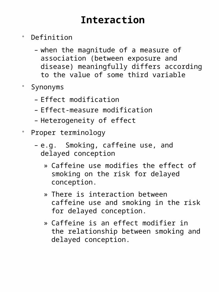
Definition
– when the magnitude of a measure of association (between exposure and disease) meaningfully differs according to the value of some third variable
Synonyms
– Effect modification
– Effect-measure modification
– Heterogeneity of effect
Proper terminology
– e.g. Smoking, caffeine use, and delayed conception
» Caffeine use modifies the effect of smoking on the risk for delayed conception.
» There is interaction between caffeine use and smoking in the risk for delayed conception.
» Caffeine is an effect modifier in the relationship between smoking and delayed conception.
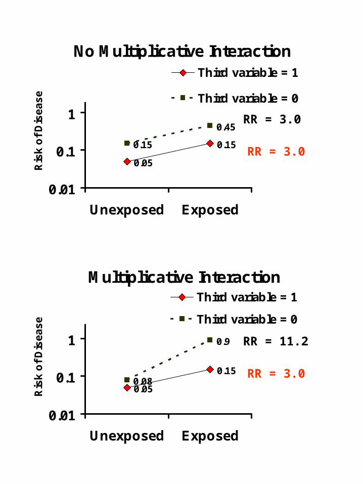
No Multiplicative Interaction
0.05
0.150.15
0.45
0.01
0.1
1
10
Unexposed Exposed
Ris
k o
f D
ise
as
e
Third variable = 1
Third variable = 0
Multiplicative Interaction
0.05
0.150.08
0.9
0.01
0.1
1
10
Unexposed Exposed
Ris
k o
f D
ise
as
e
Third variable = 1
Third variable = 0
RR = 3.0
RR = 3.0
RR = 3.0
RR = 11.2
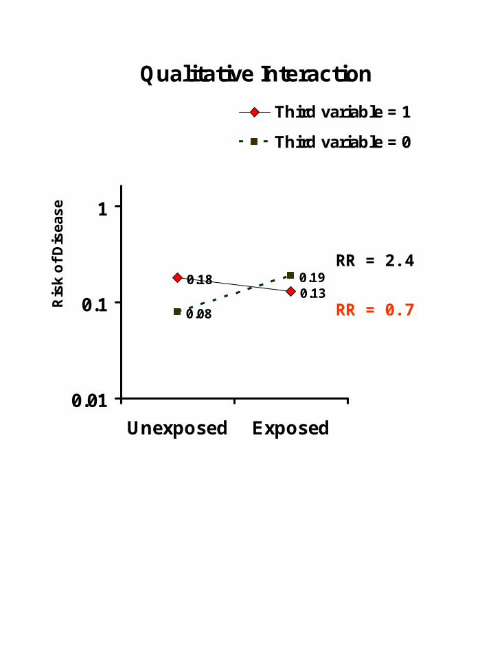
Qualitative Interaction
0.180.13
0.08
0.19
0.01
0.1
1
10
Unexposed Exposed
Ris
k o
f D
ise
as
e
Third variable = 1
Third variable = 0
RR = 0.7
RR = 2.4

Interaction is likely everywhere
Susceptibility to infectious diseases
– e.g.,
» exposure: sexual activity
» disease: HIV infection
» effect modifier: chemokine receptor phenotype
Susceptibility to non-infectious diseases
– e.g.,
» exposure: smoking
» disease: lung cancer
» effect modifier: genetic susceptibility to smoke
Susceptibility to drugs (efficacy and side effects)
» effect modifier: genetic susceptibility to drug
But in practice to date, difficult to document
– Genomics may change this

Smoking, Caffeine Use and Delayed Conception:
Additive vs Multiplicative Interaction
Delayed Not DelayedSmoking 26 133No Smoking 64 601
DelayedNot
DelayedSmoking 15 61No Smoking 47 528
Stratified
Crude
No Caffeine Use
Heavy Caffeine Use
RR crude = 1.7
RD crude = 0.07
RRno caffeine use = 2.4
RDno caffeine use = 0.12
DelayedNot
DelayedSmoking 11 72No Smoking 17 73
RRcaffeine use = 0.7
RDcaffeine use = -0.06
RD =
Risk Difference = Risk exposed - Risk Unexposed
(Text unfortunately calls this attributable risk)
Additive interaction
Multiplicative interaction
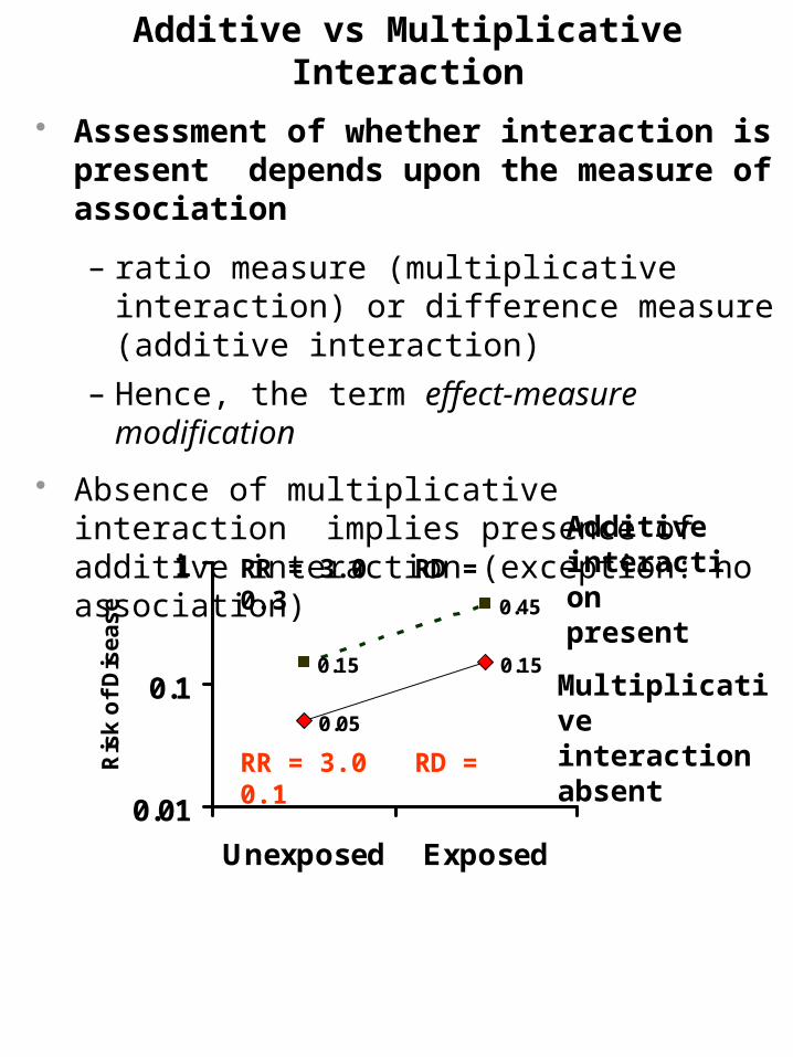
Additive vs Multiplicative Interaction
Assessment of whether interaction is present depends upon the measure of association
– ratio measure (multiplicative interaction) or difference measure (additive interaction)
– Hence, the term effect-measure modification
Absence of multiplicative interaction implies presence of additive interaction (exception: no association)
0.05
0.150.15
0.45
0.01
0.1
1
Unexposed Exposed
Ris
k o
f D
ise
as
e
Additive interaction present
Multiplicative interaction absent
RR = 3.0 RD = 0.3
RR = 3.0 RD = 0.1
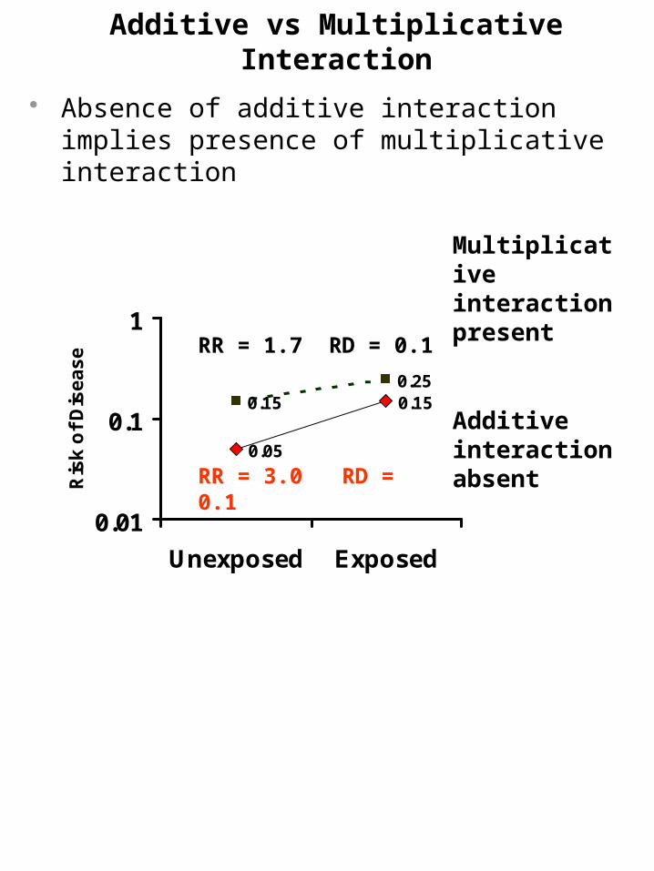
Additive vs Multiplicative Interaction
Absence of additive interaction implies presence of multiplicative interaction
0.05
0.150.150.25
0.01
0.1
1
Unexposed Exposed
Ris
k o
f D
ise
as
e
Multiplicative interaction present
Additive interaction absent
RR = 3.0 RD = 0.1
RR = 1.7 RD = 0.1

Additive vs Multiplicative Interaction
Presence of multiplicative interaction may or may not be accompanied by additive interaction
0.1
0.20.2
0.6
0.01
0.1
1
Unexposed Exposed
Ris
k o
f D
ise
as
e
0.1
0.2
0.05
0.15
0.01
0.1
1
Unexposed Exposed
Ris
k o
f D
ise
as
e
Additive interaction present
No additive interaction
RR = 2.0 RD = 0.1
RR = 2.0 RD = 0.1
RR = 3.0 RD = 0.4
RR = 3.0 RD = 0.1

Additive vs Multiplicative Interaction
Presence of additive interaction may or may not be accompanied by multiplicative interaction
0.1
0.20.2
0.6
0.01
0.1
1
Unexposed Exposed
Ris
k o
f D
ise
as
e
0.1
0.3
0.05
0.15
0.01
0.1
1
Unexposed Exposed
Ris
k o
f D
ise
as
e Multiplicative interaction absent
Multiplicative interaction present
RR = 3.0 RD = 0.1
RR = 3.0 RD = 0.4
RR = 2.0 RD = 0.1
RR = 3.0 RD = 0.2
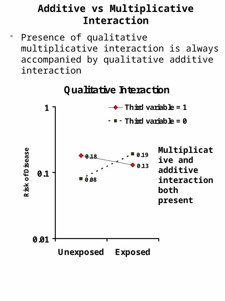
Additive vs Multiplicative Interaction
Presence of qualitative multiplicative interaction is always accompanied by qualitative additive interaction
Qualitative Interaction
0.18
0.13
0.08
0.19
0.01
0.1
1
Unexposed Exposed
Ris
k o
f D
ise
as
e
Third variable = 1
Third variable = 0
Multiplicative and additive interaction both present

Additive vs Multiplicative Scales
Which do you want to use?
Multiplicative measures (e.g., risk ratio)
– favored measure when looking for causal association (etiologic research)
– not dependent upon background incidence of disease
Additive measures (e.g., risk difference):
– readily translated into impact of an exposure (or intervention) in terms of absolute number of outcomes prevented
» e.g. 1/risk difference = no. needed to treat to prevent (or avert) one case of disease
or no. of exposed persons one needs to take the exposure away from to avert one case of disease
– very dependent upon background incidence of disease
– gives “public health impact” of the exposure
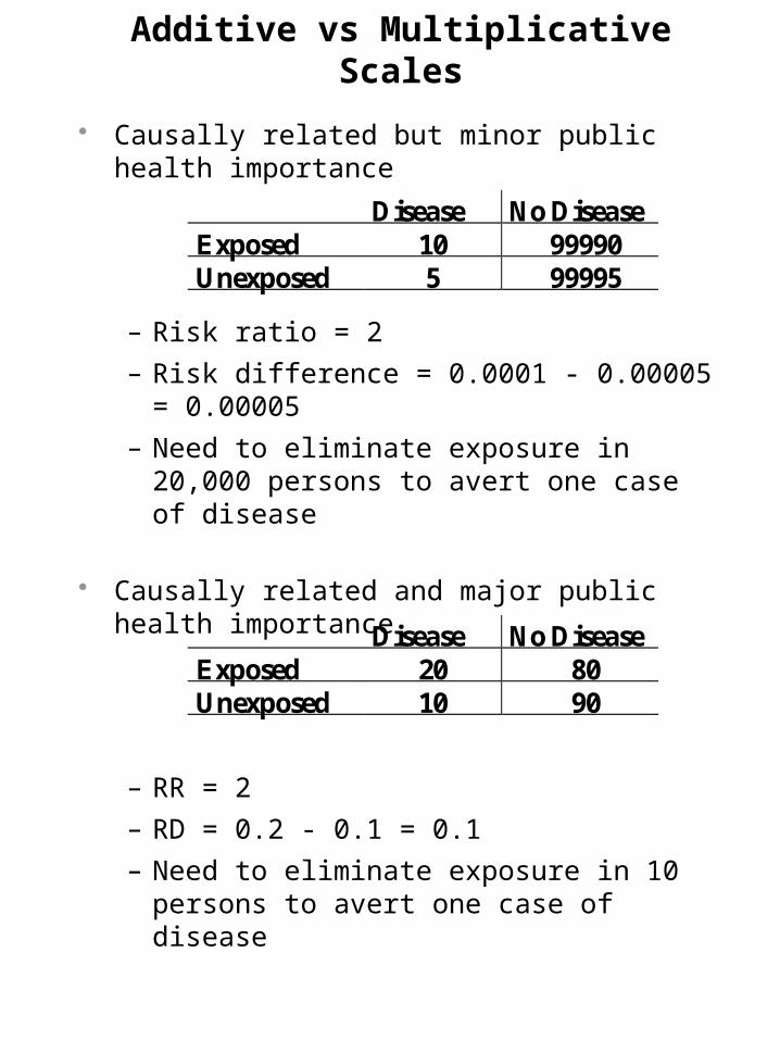
Additive vs Multiplicative Scales
Causally related but minor public health importance
– Risk ratio = 2
– Risk difference = 0.0001 - 0.00005 = 0.00005
– Need to eliminate exposure in 20,000 persons to avert one case of disease
Causally related and major public health importance
– RR = 2
– RD = 0.2 - 0.1 = 0.1
– Need to eliminate exposure in 10 persons to avert one case of disease
Disease No DiseaseExposed 10 99990Unexposed 5 99995
Disease No DiseaseExposed 20 80Unexposed 10 90

Smoking, Family History and Cancer:
Additive vs Multiplicative Interaction
Cancer No CancerSmoking 50 150No Smoking 25 175
CancerNo
CancerSmoking 10 90No Smoking 5 95
Stratified
Crude
Family History Absent
Family History Present
Risk rationo family history = 2.0
RDno family history = 0.05
CancerNo
CancerSmoking 40 60No Smoking 20 80
Risk ratiofamily history = 2.0
RDfamily history = 0.20
• No multiplicative interaction but presence of additive interaction
• If etiology is goal, risk ratio is sufficient
• If goal is to define sub-groups of persons to target:
- Rather than ignoring, it is worth reporting that only 5 persons with a family history have to be prevented from smoking to avert one case of cancer

Confounding vs Interaction
We discovered interaction by performing stratification as a means to get rid of confounding
– This is where the similarities between confounding and interaction end!
Confounding
– An extraneous or nuisance pathway that an investigator hopes to prevent or rule out
Interaction
– A more detailed description of the relationship between the exposure and disease
– A richer description of the biologic or behavioral system under study
– A finding to be reported, not a bias to be eliminated

Smoking, Caffeine Use and Delayed Conception
Delayed Not DelayedSmoking 26 133No Smoking 64 601
DelayedNot
DelayedSmoking 15 61No Smoking 47 528
Stratified
Crude
No Caffeine Use
Heavy Caffeine Use
RR crude = 1.7
RRno caffeine use = 2.4
DelayedNot
DelayedSmoking 11 72No Smoking 17 73
RRcaffeine use = 0.7
RR adjusted = 1.4 (95% CI= 0.9 to 2.1)
Is this the best “final” answer?
Here, adjustment is contraindicated
When interaction is present, confoundng becomes irrelevant!
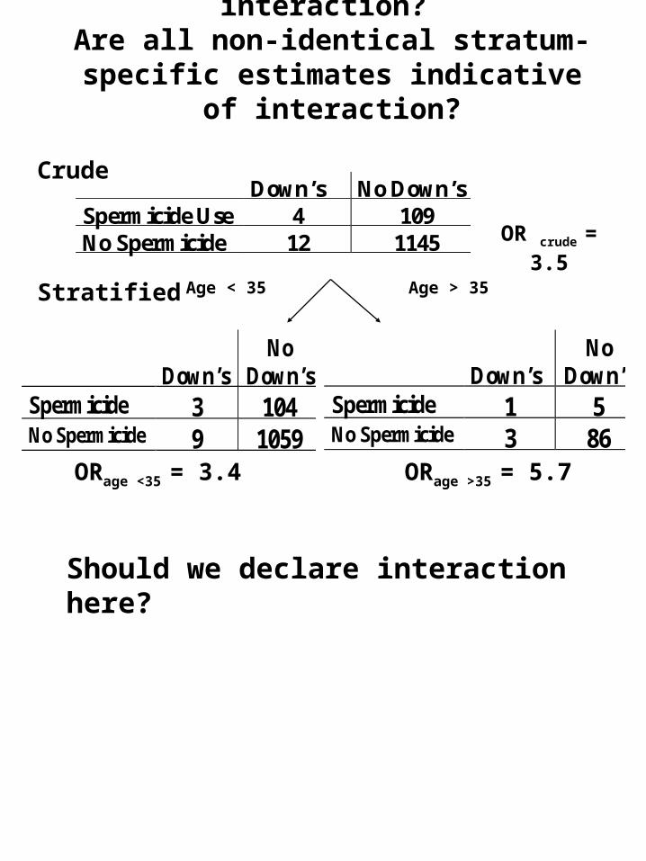
Chance as a cause of interaction? Are all non-identical stratum-specific estimates indicative of interaction?
Down’s No Down’sSpermicide Use 4 109No Spermicide 12 1145
Down’sNo
Down’sSpermicide 3 104No Spermicide 9 1059
Stratified
Crude
Age > 35Age < 35
OR crude = 3.5
ORage >35 = 5.7
Down’sNo
Down’sSpermicide 1 5No Spermicide 3 86
ORage <35 = 3.4
Should we declare interaction here?

Statistical Tests of Interaction: Test of Homogeneity (heterogeneity)
Null hypothesis: The individual stratum-specific estimates of the measure of association differ only by random variation (chance or sampling error)
– i.e., the strength of association is homogeneous across all strata
– i.e., there is no interaction
A variety of formal tests are available with the same general format, following a chi-square distribution:
where:
– effecti = stratum-specific measure of assoc.
– var(effecti) = variance of stratum-specifc m.o.a.
– summary effect = summary adjusted effect
– N = no. of strata of third variable
For ratio measures of effect, e.g., OR, log transformations are used:
The test statistic will have a chi-square distribution with degrees of freedom of one less than the number of strata
i i
iN effect
effectsummaryeffectsquarechi
)var(
) ( 2
1
Interpreting Tests of Homogeneity
If the test of homogeneity is “significant”, we reject the null in favor of the alternative hypothesis
– this is evidence that there is heterogeneity (i.e. no homogeneity)
– i.e., interaction may be present
The choice of a significance level (e.g. p < 0.05) for reporting interaction is not clear cut.
– There are inherent limitations in the power of the test of homogeneity
» p < 0.05 may be too conservative
– One approach is to report interaction for p < 0.10 to 0.20 if the magnitude of differences is high enough
» i.e., if it is not too complicated to report stratum-specific estimates, it is often more revealing to report potential interaction than to ignore it.
» However, meaning of p value is not different than other contexts
» Not a purely statistical decision

Tests of Homogeneity with Stata
1. Determine crude measure of association
e.g. for a cohort study
command: cs outcome-variable exposure-variable
for smoking, caffeine, delayed conception:
-exposure variable = “smoking”
-outcome variable = “delayed”
-third variable = “caffeine”
command is: cs delayed smoking
2. Determine stratum-specific estimates by levels of third variable
command:
cs outcome-var exposure-var, by(third-variable)
e.g. cs delayed smoking, by(caffeine)

. cs delayed smoking
| smoking | | Exposed Unexposed | Total
-----------------+------------------------+----------
Cases | 26 64 | 90
Noncases | 133 601 | 734
-----------------+------------------------+----------
Total | 159 665 | 824
| |
Risk | .163522 .0962406 | .1092233
| Point estimate | [95% Conf. Interval]
|------------------------+----------------------
Risk difference | .0672814 | .0055795 .1289833
Risk ratio | 1.699096 | 1.114485 2.590369
– +----------------------------------------------- chi2(1) = 5.97 Pr>chi2 = 0.0145
. cs delayed smoking, by(caffeine)
caffeine | RR [95% Conf. Interval] M-H Weight
-----------------+-------------------------------------------------
no caffeine | 2.414614 1.42165 4.10112 5.486943
heavy caffeine | .70163 .3493615 1.409099 8.156069
-----------------+-------------------------------------------------
Crude | 1.699096 1.114485 2.590369
M-H combined | 1.390557 .9246598 2.091201
-----------------+-------------------------------------------------
Test of homogeneity (M-H) chi2(1) = 7.866 Pr>chi2 = 0.0050
What does the p value mean?

Report vs Ignore Interaction?Some Guidelines
Risk Ratios for a Given Exposure and Disease
Potential Effect Modifier Present Absent
P value for heterogeneity
Report or Ignore
Interaction
2.3 2.6 0.45 Ignore
2.3 2.6 0.001 Ignore
2.0 20.0 0.001 Report
2.0 20.0 0.20 Report
2.0 20.0 0.40 Ignore
3.0 4.5 0.30 Ignore
3.0 4.5 0.001 +/-
0.5 3.0 0.001 Report
0.5 3.0 0.20 Report
0.5 3.0 0.30 +/-
Is an art form: requires consideration of both clinical and statistical significance

When Assessing the Association Between an Exposure and a Disease,
What are the Possible Effects of a Third Variable?
EM+
_Confounding:
ANOTHER PATHWAY TO
GET TO THE DISEASE
Confounding:
ANOTHER PATHWAY TO
GET TO THE DISEASE
Effect Modifier (Interaction):
MODIFIES THE EFFECT OF THE EXPOSURE
D
I C
Intermediary
Variable:
No Effect
ON CAUSAL PATHWAY


![How Algorithmic Confounding in Recommendation Systems ... · Bias, confounding, and estimands. Schnabel, et al. [52] note that users introduce selection bias; this occurs during the](https://static.fdocuments.net/doc/165x107/5edf75ccad6a402d666aceb0/how-algorithmic-confounding-in-recommendation-systems-bias-confounding-and.jpg)