The Conflict Trap∗

Havard Hegre1,2, Havard Mokleiv Nygard1,2, Havard Strand1, Scott Gates1,3, and RanveigD. Flaten2

1Centre for the Study of Civil War, PRIO2Department of Political Science, University of Oslo

3Norwegian University of Science and Technologies, NTNU

October 11, 2011

Abstract

Several studies indicate that internal armed conflict breeds conflict. Armed conflict creates conditionsthat increase the chances of war breaking out again. This ‘conflict trap’ works through several channels:Conflicts (1) polarize populations and create deep resentments and build up the organizational capacityfor future warfare, (2) undermine democratic political institutions, and (3) exacerbate the conditionsthat favor insurgency by increasing poverty, causing capital flight, destabilizing neighboring countries etc.This study quantifies the total effect of the conflict trap more precisely than in earlier studies by meansof a transition model and extensive use of simulations to estimate the total effect over long time periodsand across countries.

∗Prepared for the 2011 Annual Meeting of the American Political Science Association in Seattle, WA. The paper builds onthe simulation framework developed in Hegre et al. (forthcoming) and the simulation program developed by Joakim Karlsen.

1

1 Introduction

In any year over the last decade, 25–30 countries in the world had an internal armed conflict – an armed

confrontation between the government and an organized opposition group. These conflicts are not distributed

randomly across the globe. They disproportionally occur in a group of about 50 countries, or in ‘the bottom

billion’ population of the world (Collier, 2007). A partial reason for this clustering is that the structural

factors that tend to facilitate conflict – poverty, poor governance, and non-participation in the modern,

global economy – are clustered. This clustering, however, is intensified by the ‘conflict trap’ (Collier et al.,

2003). Conflicts tend to aggravate these structural forces, polarize societies, and erode societies’ ability to

handle conflict without violence, thereby increasing the risk of future conflict in the country as well as in its

neighborhood.

In this paper we seek to assess how intense this conflict trap is. Our point of departure is a statistical

model of what determines the risk of armed conflict along the lines of studies such as Fearon and Laitin (2003),

Collier, Hoeffler and Soderbom (2004), or Cederman, Hug and Krebs (2010). These studies typically record

available information for countries once every year, and report how variables of interest such as democracy

or ethnic fragmentation increase or decrease the risk of onset or termination of conflict in a given year.

Assessing the conflict trap is more demanding, however, since the ‘trapping effects’ extend far beyond

the country year for which we have direct statistical estimates – they involve a set of factors active over a

significant period of time, and working through several channels. Here lies a dilemma – in order to obtain

precise estimates, we need to analyze relatively disaggregated units of analysis, but this poses a challenge

when the aim is to conclude at a more aggregated level.

Here, we use the simulation tools developed in Hegre et al. (forthcoming) to assess how the outbreak of

conflicts tend to affect the risk of future conflict in the same countries, its neighborhood, and even globally.

Since the conflict trap is related to both onset, termination, and recurrence of conflict, we study the incidence

of conflict, simultaneously assessing the determinants of onset and duration of conflict (Bleaney and Dimico,

2011). In our specification, we carefully model how the risk of conflict depends on former conflict in the

country itself as well as its neighborhood. The simulation takes the estimated model of the risk of conflict

incidence as its point of departure, calculates the probabilities of onset, termination, and recurrence of conflict,

and simulates a set of possible future trajectories of conflict based on these probabilities. These simulations

are accurate representations of the view of the world reflected in our statistical model, and close to the views

of the world presented in similar studies of armed conflict.

To assess the intensity of the conflict trap, we conduct a set of ‘experiments’ within our simulations. For

instance, we investigate the model’s implications for the future risk of conflict if a conflict was to break out

in 2009 in a previously peaceful country. For poor countries – one of the bottom billion ones – such an onset

would increase the risk of conflict considerably for several decades. The implications are obvious – if anything

can be done to prevent the onset of conflict in such a country, it will have positive effects far beyond the

immediate situation. Conversely, we demonstrate that a successful cessation of hostilities for a year in an

2

ongoing conflict reduces the future incidence of conflict over the next 2–3 decades.

In the next phase of this project, we will use the methodology to assess how important the economic

impact of conflict is for the conflict trap. We do this by entering a model for how GDP per capita reacts to

conflict into the simulation procedure [not yet implemented at the time of writing].

In the next section, we look at some simple statistics related to the conflict trap. In section 3, we review

the literature. In section 4 we account for the statistical model, and in section 5 we present the simulation

technique and the simulation results. In section 6 we look into how the various sources of the conflict trap

can be identified.

2 The conflict trap

What do we mean by the ‘conflict trap’, and how important is it?

We speak of a ‘conflict trap’ if the long-term risk of conflict in a country or region increases considerably

after the first conflict onset. Within a country, the conflict trap may manifest itself as a tendency for

conflicts to be very long even in countries with no previous conflict, a high risk of recurrence after conflicts

are terminated, or as spill-over from conflicts in neighboring countries, or a combination of all of these.

A more precise definition requires a definition of conflict. We use that of the Uppsala Conflict Data Project

(UCDP), and our data are from the 2010 update of the UCDP/PRIO Armed Conflict Dataset (Harbom and

Wallensteen, 2010; Gleditsch et al., 2002). This dataset records conflicts at two levels. Minor conflicts are

those that pass the 25 battle-related deaths threshold but have less than 1000 deaths in a year. Major

conflicts are those conflicts that pass the 1000 annual deaths threshold. We only look at internal armed

conflicts, and only include the countries whose governments are included in the primary conflict dyad (i.e.,

we exclude other countries that intervene in the internal conflict). The conflict countries in 2009 are shown

in Figure 1.

2.1 Descriptive conflict statistics

Figure 2 shows Kaplan-Meier survival estimates of ‘conflict spell’ duration. Here, we define a conflict spell

as a set of consecutive years with at least 25 battle-related deaths per year, within a given country. There

were a total of 245 conflict spell onsets in the world between 1945 and 2009, taking place in 102 different

countries. 76 of the countries included in our study did not have any conflicts at all during this period, and

39 countries had only one conflict spell. The left panel shows the survival statistics of all conflict countries,

and the right panel those of three selected regions: South and Central America and the Caribbean (‘the

Americas’), West-Africa and Eastern, and South-East Asia.1 The average duration of a conflict was 5.2 years

and the median was 2 years, but a large fraction of the conflict spells last for 10–20 years or longer. Eastern

1The Kaplan-Meier estimator is a non-parametric estimate of the survivor function, which in this case represents how longa country remains in conflict, before it manages to break out of it. More precisely, it gives an estimate of the probability ofremaining in conflict after a certain time, t, measured in years after the last conflict outbreak.

3

Figure 1: Map of conflicts ongoing in 2009

LegendNo ConflictMinor ConflictMajor Conflict

Source: Harbom and Wallensteen (2010)

and South East Asia, as figure 2 shows, has a higher probability of protracted conflict periods than do West

Africa and the Americas.

Figure 2: Kaplan Meier Survival Estimates: Conflict duration

Many conflicts are restricted to a single ‘spell’. The group of ‘one-spell countries’ is quite diverse; some

have had long and protracted wars lasting for decades, like Colombia (1964–) and Afghanistan (1978–),

whereas many others only experienced one or a few years of conflict, like for example the Dominican Republic

in 1965 or Gambia in 1981.

The conflict trap also manifests itself as the experience of several conflict spells, lasting for one or several

years. In between these conflict-periods we find shorter or longer spells of peace. Columns 4 and 5 of Table

There were 143 ‘post-conflict spells’ (i.e. a new conflict outbreak after a period of minimum one year of

4

Table 1: Overview of countries with multiple conflicts

Region (countries in total) Conflict Minor Major Average durationcountries conflict conflict duration

South and Central America and the Caribbean (27) 11 26 4 3.5Western Europe, N. America and Oceania (27) 3 7 - 4.86Eastern Europe (20) 3 4 4 3.5Western Asia and North Africa (22) 10 23 8 5.32West Africa (17) 7 24 - 1.88East, Central and Southern Africa (38) 14 47 6 4.45South and Central Asia (12) 6 19 6 5.12Eastern and South-East Asia (19) 9 15 13 8.60Total 63 165 41 5.03

Figure 3: Kaplan Meier Survival Estimates: Post-conflict peace

post-conflict peace) between 1945 and 2009, taking place in 63 different countries. 123 of these were minor

conflicts and 20 were major conflicts. Table 1 gives an overview of countries with multiple conflict spells.

We find the longest repeated spells in East and South-East Asia with an average duration of 8.6 years.

West-Africa, on the other hand, only had an average of 1.88 years throughout the period.

The average post-conflict time at peace was 10.6 years and the median time was 6 years.2 There are a

total of 215 country-conflict observations, or subjects at risk, defined from the year after the first conflict in

a country ended.3

Figure 3 shows Kaplan-Meier survival estimates of post-conflict peace, one for all post-conflict countries,

and one which highlights the difference in post-conflict peace-time in the same three regions. In this case the

survivor function represents how long a country emerging from a conflict remains at peace before entering

into a new conflict. South and Central Asia and the African countries clearly have steeper curves than do

the South and Central American and Caribbean countries – they are more prone to falling back into conflict

at an earlier point in time.

2We find countries that have experienced everything from a minimum of 1 year to a maximum of 60 years.3Countries such as Colombia that remain in their first conflict to the end of the dataset will never enter the risk post-conflict

peace risk set.

5

Figure 4: Scalar Index of Polities (SIP), GDP per capita and Conflict, 1969-2009

3 Why there is a conflict trap

Collier et al. (2003, ch. 4) argues that this ‘conflict trap’ comes about through several channels: Conflicts (1)

polarize populations and create deep resentments and build up the organizational capacity for future warfare,

(2) undermine democratic political institutions, and (3) exacerbate the conditions that favor insurgency by

increasing poverty, causing capital flight, destabilizing neighboring countries etc.

3.1 Growth of ‘conflict capital’

Experiencing civil war drastically increases the risk of renewed occurrences of civil war within the same

country and in neighboring countries (Hegre et al., 2001; Collier, Hoeffler and Soderbom, 2008; Quinn,

Mason and Gurses, 2007; Walter, 2004). Civil war is also regularly associated with large-scale violence

against civilians (Eck and Hultman, 2007). Collier, Hoeffler and Soderbom (2008) estimate the risk of

conflict reversal to be around 40% during the first post-conflict decade, and Elbadawi, Hegre and Milante

(2008) find an even higher rate using a more inclusive definition of conflict.4

4See Suhrke and Samset (2007) for a critical discussion of this figure.

6

Collier et al. (2003, ch. 4) points to several sources of a conflict trap. The most important is the fact that

war destroys economic development, reviewed in detail below. Moreover, diaspora communities have in several

cases contributed to the continuation of conflict through financing of extremist groups in their homelands.

Conflict, moreover, strengthens a military lobby, contributing to excessive and counter-productive military

spending. The military organization built by rebel groups increases the incentives for the opposition to use

military force in the future.

Another part of the mechanism is the human factor. A post-conflict society is often marked by anger and

hate among victims of the conflict on the one hand, and a comptance in war-waging among veterans on the

other hand. The motive and opportunity for future conflict is very much present in the mind of the public,

in a way that cannot be captured by a stuctural variable like GDP/capita or democracy. There is little

systematic research on this factor, but an interesting fact highlights one of these factors: When a conflict

ends in a clear defeat for one of the parties, the likelihood of recurrence is significantly lower than for all

other forms of termination Kreutz (2010). In these scenarios, the supply of capable veterans are probably

lower.

These studies, however, often fail to acknowledge that conflicts have strong adverse effects on major

conflict risk factors. In particular, conflicts may have a strongly adverse impact on average income, which

is a key factor associated with conflict onset. Collier et al. (2003, ch. 4) show that there is a ‘conflict trap’

tendency. They estimate that about half of all post-conflict countries return to conflict. A third of the

post-conflict countries succeed in keeping the peace beyond the first 10 years, but these enter a category

classified as ‘marginalized countries at peace’ (roughly the same as the ‘bottom billion’ countries without

conflict; cf. Collier, 2007). This group of countries is characterized by low incomes and sluggish growth, and

has a markedly higher risk of conflict than other countries. Only one sixth of post-conflict countries end up

in the group of ‘successful developers’, drastically reducing conflict risk (Collier et al., 2003, 109).

3.2 The effect of armed conflict on economic growth

The conflict trap channel that has received most attention in the literature is conflict’s impact on economic

growth and diversification. Figure 4 shows some examples of the economic effects of conflict. For each of nine

countries in East Africa, we show average GDP per capita (dashed line) and democracy (dot-dashed line) in

the main, upper panel. In the lower panel, conflicts (dark grey bars) and conflicts in the neighborhood (light

grey bars) are shown. Uganda, Burundi, Rwanda, the Democratic Republic of Congo, and Mozambique all

saw substantial economic decline during the first years of their conflicts.

War affects the economy of a country in a number of ways. Financing the war itself is costly. How the war is

paid for in the short run can lead to inflation. Trade and finance are also disrupted. But most fundamentally,

war destroys. Buildings and infrastructure are demolished. Valuable human capital is destroyed in death

and injury or lost in the form of refugees fleeing from the carnage. Such luminaries of economics as Pigou

(1916; 1921) and Keynes (1919) studied the interactions between war, peace and economics. These early

7

works focused almost exclusively on the economic consequences of interstate wars.

Recent work has focused more on armed civil conflict, which occurs with considerably greater frequency

than interstate conflict. Collier (1999) distinguishes the differences between interstate and intrastate conflict,

arguing that civil wars are ‘liable to be more damaging than international wars’. As might be expected,

economic costs of civil war are found to be associated with the geographical extent of the conflict and the

destruction of the human and capital stock; the general disruption of commerce; and the disruption of

the government’s capacity to collect revenues and provide essential services. Moreover, following Collier’s

analysis, ‘a broad consensus has emerged that civil conflict reduces annual real GDP growth by about 2

percentage points’ (Staines, 2004).5

Indeed, Gates et al. (2010) in their systematic analysis of the economic consequences of civil conflict,

like Collier, find a 2% reduction in economic growth, but only from major armed conflicts, or civil wars.

For minor conflicts Gates et al. (2010) find no significant effect. This probably reflects several concurrent

tendencies. In very unstable countries, a high likelihood of minor instances of political violence, such as coups

or short armed conflicts, are probably included into the calculation of key economic actors before they occur.

Moreover, minor conflicts in large countries such as India are unlikely to affect the Indian economy at large.

Koubi (2005) studies the effect of both inter- and intranational wars on average growth in per capita

real output. She finds that a war’s severity, measured in battle deaths, has a significant negative impact

on growth. When she conducts the analysis for interstate wars only, the statistical significance disappears,

indicating that the ‘association between war and economic growth is due to civil wars’ (Koubi, 2005, 76–77).

Collier (1999) also examined the differential effects of war duration. He finds that while short wars ‘cause

continued post-war [GDP] decline, [...] sufficiently long wars give rise to a phase of rapid growth’ (Collier,

1999, p. 175–176), reflecting a ‘Phoenix effect’ (Organski and Kugler, 1980). The continued decline in GDP

after short wars Collier attributes to post-war environments being less capital-friendly than that country’s the

pre-war capital environment. Indeed, capital flight is a big problem in post-conflict environments (Davies,

2008). Koubi (2005, 78) also finds that ‘the more severe or longer the war, the higher the subsequent,

medium-term economic growth’. Similarly, Chen, Loayza and Reynal-Querol (2008, p. 71) find that the

‘average level of per capita GDP is significantly lower after the war than before it’, and this they argue is

‘undoubtedly a direct reflection of the cost of war’. They, too, find that after ‘the destruction from war,

recovery is achieved through above average growth’ but this growth follows the pattern of ‘an inverted U,

with the strongest results achieved in the fourth or fifth year after the onset of peace’ (Chen, Loayza and

Reynal-Querol, 2008, p. 72, 79). Likewise, Blomberg, Hess and Thacker (2000) find a strong negative effect

of both external and internal conflict on growth. Flores and Nooruddin (2009) examine the special problems

democracies face when trying to implement economic policy reforms in a post-conflict environment.

The economic effects of civil war also tend to spill over into neighboring countries (Buhaug and Gleditsch,

2008; Gleditsch and Ward, 2000; Salehyan and Gleditsch, 2006). Murdoch and Sandler (2002) and Murdoch

5Collier (1999, p. 175–176) claims more precisely, that after ‘civil war the annual (GDP) growth rate is reduced by 2.2%’.

8

and Sandler (2004) focus on the spillover effects from conflicts in neighboring countries and the magnified

costs of being located near a more widespread set of wars that constitute a regional conflict. Murdoch and

Sandler (2002, p. 96) contend that a neighboring civil war affects GDP directly and indirectly. The direct

effect is from the collateral damage whereby battles close to the border destroy infrastructure and capital.

the indirect effect occurs by increasing the ‘perceived risk to would-be investors and divert foreign direct

investment away from neighbors at peace’. They further find that a civil war creates ‘significant negative

influence on short-run growth within the country and its neighbors’ (Murdoch and Sandler, 2002, p. 106–07).

In Murdoch and Sandler (2004) they argue ‘owing to regional economic integration and regional multiplier

effects’, the spillover effects may go beyond a country’s immediate neighbors. For neighbors within a radius

of 800 km they find that ‘a civil war at home is associated with a decline in economic growth of 0.1648, while

and additional civil war in a neighbor is associated with a decline of approximately 0.05 or about 30 % of the

home-country effect’ (Murdoch and Sandler, 2004, 145). This implies that ‘a country in a region with three

or more civil wars may be equally impacted as a country experiencing a civil war” (Murdoch and Sandler,

2004, 150).

Poverty is among the most important structural conditions that facilitate internal armed conflict (Collier

and Hoeffler, 2004; Fearon and Laitin, 2003; Hegre and Sambanis, 2006). The detrimental effect of conflict

on the economy, then, increases the risk of continued or renewed conflict. Adding to this, armed conflict

also adversely affects the structure of the economy. Since land-specific capital such as agriculture and other

primary commodity extraction is less mobile, conflict transforms societies into more primary-commodity

dependent economies (Collier et al., 2003, 84). Such economies are arguably more vulnerable to conflict and

authoritarian politics (Collier and Hoeffler, 2004; Boix, 2003).

3.3 The effect of armed conflict on democracy

Surprisingly little systematic comparative research has examined the political consequences of civil war. The

most common work focuses on human rights violations as they relate to civil war. Indeed, a common finding

in empirical studies of human rights violations is that personal integrity abuse is highly associated with civil

war (Poe, Tate and Keith, 1999; Davenport, 2007). Others have found that a surge in human rights abuses

and restrictions on civil liberties tend to occur after civil wars (Zanger, 2000; Colaresi and Carey, 2008).

The role that armed civil conflict plays in state development has been subjected to considerable theoretical

speculation (Tilly, 1975; Holsti, 1996; Bates, 2001). Indeed, warfare and preparations for war have served

‘to promote territorial consolidation, centralization, differentiation in the instruments of government, and

monopolization of the means of coercion, all the fundamental state-making processes. War made the state

and the state made war’ (Tilly, 1975, p. 42). While the theoretical work on state development is rich, there

is almost no extensive empirical analysis. Nevertheless, some empirical work has begun to shed light on the

relationship between war and aspects of the state. For example Collier et al. (2003) and Hegre, Elbadawi and

Milante (2007) offer evidence that war results in the centralization of authority. A related body of research

9

examines the endogeneity of democratization and interstate war (Mitchell, Gates and Hegre, 1999; Bueno de

Mesquita, Siverson and Woller, 1992; Thompson, 1996; Rasler and Thompson, 2004). Another set of studies

focus on the effect of interstate war on leadership tenure (Goemans, 2000; Bueno de Mesquita and Siverson,

1995), but few if any studies have looked at these issues with regard to civil war.

Figure 4 indicates a more ambiguous effect of conflict on a country’s political system. In several of

these East/Central African cases, conflict was associated with the demise of an authoritarian system (e.g.,

in Uganda, Burundi, and Rwanda). In Mozambique, a substantial democratization followed the termination

of the conflict.

4 Estimating the conflict trap

4.1 Statistical model

We include information on three different conflict states from the UCDP/PRIO dataset – no conflict, minor,

or major conflict. To assess the conflict trap statistically, it is necessary to have a model that is able to

estimate all the transition probabilities between the states of no conflict, minor conflict, and major conflict.

One may estimate this matrix of transition probabilities using a multinomial logit model with the conflict

level at t as the outcome variable, and the level at t−1 as a set of dummy variables. This type of model may

be referred to as a ‘dynamic multinomial model’ or a ‘Markov Model’ (Amemiya, 1985).6 In the multinomial

model (see Greene, 1997, 914–917) for the three outcomes (j = 0 : ‘no conflict’, j = 1 : ‘minor conflict’,

j = 2 : ‘major conflict’), the probabilities of the three outcomes are given by:

p(Yi = j) =exβj∑2k=0 e

xβk

(1)

To identify the model, we set ‘no conflict’ as the base outcome. The estimates β1 reported below, then, are

interpreted as the impact of the explanatory variable on the probability of being in ‘minor conflict’ relative

to ‘no conflict’. The β2 estimates approximate the probability of ‘major conflict’ relative to ‘no conflict’.

In addition to variables denoting the state at t − 1 as explanatory variable(s) (i.e., lagged dependent

variables), the model accounts for a set of explanatory variables, discussed in section 4.3. The estimates for

the lagged dependent variables and the constant terms then estimate the transition probability matrix for

the case where all explanatory variables are zero. The model allows capturing variables that may increase

the risk of conflict onset, but not its duration, by adding interaction terms between the state at t − 1 and

predictor variables.

6Przeworski et al. (2000), for instance, refer to their related model as a dynamic probit model.

10

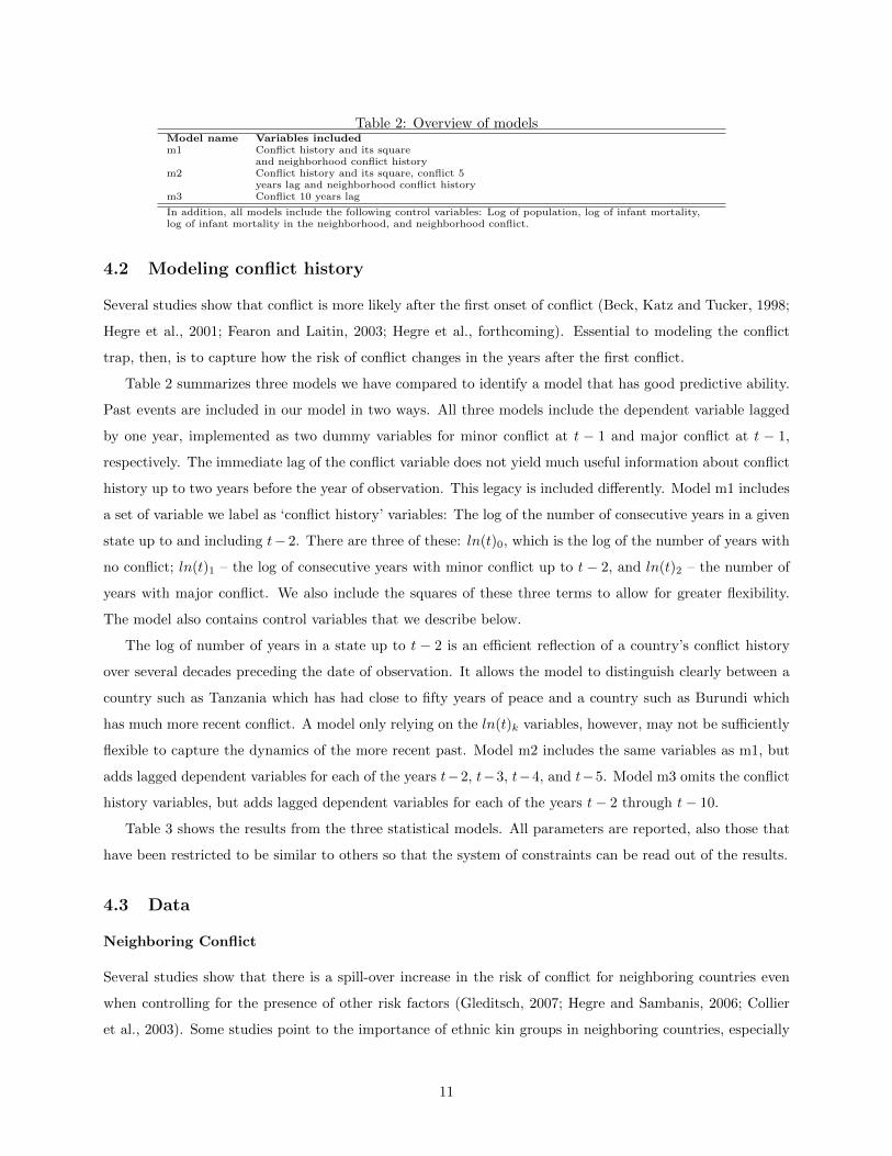
Table 2: Overview of modelsModel name Variables includedm1 Conflict history and its square

and neighborhood conflict historym2 Conflict history and its square, conflict 5

years lag and neighborhood conflict historym3 Conflict 10 years lag

In addition, all models include the following control variables: Log of population, log of infant mortality,log of infant mortality in the neighborhood, and neighborhood conflict.

4.2 Modeling conflict history

Several studies show that conflict is more likely after the first onset of conflict (Beck, Katz and Tucker, 1998;

Hegre et al., 2001; Fearon and Laitin, 2003; Hegre et al., forthcoming). Essential to modeling the conflict

trap, then, is to capture how the risk of conflict changes in the years after the first conflict.

Table 2 summarizes three models we have compared to identify a model that has good predictive ability.

Past events are included in our model in two ways. All three models include the dependent variable lagged

by one year, implemented as two dummy variables for minor conflict at t − 1 and major conflict at t − 1,

respectively. The immediate lag of the conflict variable does not yield much useful information about conflict

history up to two years before the year of observation. This legacy is included differently. Model m1 includes

a set of variable we label as ‘conflict history’ variables: The log of the number of consecutive years in a given

state up to and including t− 2. There are three of these: ln(t)0, which is the log of the number of years with

no conflict; ln(t)1 – the log of consecutive years with minor conflict up to t− 2, and ln(t)2 – the number of

years with major conflict. We also include the squares of these three terms to allow for greater flexibility.

The model also contains control variables that we describe below.

The log of number of years in a state up to t − 2 is an efficient reflection of a country’s conflict history

over several decades preceding the date of observation. It allows the model to distinguish clearly between a

country such as Tanzania which has had close to fifty years of peace and a country such as Burundi which

has much more recent conflict. A model only relying on the ln(t)k variables, however, may not be sufficiently

flexible to capture the dynamics of the more recent past. Model m2 includes the same variables as m1, but

adds lagged dependent variables for each of the years t−2, t−3, t−4, and t−5. Model m3 omits the conflict

history variables, but adds lagged dependent variables for each of the years t− 2 through t− 10.

Table 3 shows the results from the three statistical models. All parameters are reported, also those that

have been restricted to be similar to others so that the system of constraints can be read out of the results.

4.3 Data

Neighboring Conflict

Several studies show that there is a spill-over increase in the risk of conflict for neighboring countries even

when controlling for the presence of other risk factors (Gleditsch, 2007; Hegre and Sambanis, 2006; Collier

et al., 2003). Some studies point to the importance of ethnic kin groups in neighboring countries, especially

11

in conjunction with significant refugee flows (Salehyan and Gleditsch, 2006). Others argue that detrimental

economic effects of conflict contaminate neighbors (Murdoch and Sandler, 2004).

We define the neighborhood of a country A as all N countries [B1...Bn] that share a border with A, as

defined by Gleditsch and Ward (2000). More specifically, we define ‘sharing a border’ as having less than 100

km between any points of their territories. The spatial lag of conflict is a dummy variable measuring whether

there is conflict in the neighborhood or not. Since the dependent variable is nominal, we construct two spatial

lags: one for minor conflicts and one for major conflicts. Islands with no borders are considered as their own

neighborhood when coding the exogenous predictor variables, but have by definition no neighboring conflicts.

Since our aim is to predict, we are best served by a spatial lag of conflict as our measure of neighborhood

effects. In our estimated models, we rely on observed levels of conflict in the direct neighborhood of each

country. In our simulation models, we update these variables based on the simulated results – if a conflict is

simulated to erupt, the values for the neighboring countries change.

Infant Mortality Rates

Infant mortality rates (IMR) has been promoted as an alternative measure of level of development (Goldstone,

2001), capturing a broader set of developmental factors than the standard measure of income levels (GDP

per capita). Esty et al. (1998) report very strong effects of infant mortality on state failure and conflict.

Urdal (2005) and Abouharb and Kimball (2007) find high infant mortality rates to be strongly associated

with an increased risk of armed conflict onset. Generally, infant mortality appears to perform very similar

to other measures of general development.7

IMR is defined as the probability of dying between birth and exact age 1 year, expressed as the number

of infant deaths per 1000 live births. Our data are taken from the UN Population Division (United Nations,

2007), who also provides a projection up to 2050 that we use as forecast for the predictor. Given the con-

siderable fluctuations in infant mortality associated with different economic, social, and political conditions,

it is plausible to expect significant uncertainty associated with future trends. We assume that the marginal

effect of infant mortality rates on conflict is decreasing, so in the estimation we include the log of the variable.

Population

Greater populations are associated with increased conflict risks. A country with the population size of

Nigeria has an estimated risk that is about 3 times higher than a country the size of Liberia.8 The increase

in the risk of conflict does not increase proportionally with population, however. The per-capita risk of civil

7Per-capita income is among the most robust predictors of internal armed conflict. Almost all scholars find it to be associatedwith a high risk of the onset of conflict (Hegre and Sambanis, 2006), and GDP per capita is included in virtually all studies of therisk of armed conflict onset. In the models estimated below, we do not include income as a variable. This is partly because wedo not have access to good projections for this variable, partly because education levels, infant mortality rates, and per-capitaincome are so highly correlated.

8This is based on an log-odds estimate of 0.3, typical for cross-national logistic regression models with a log populationvariable. See Raleigh and Hegre (2009) for references and a discussion.

12

war decreases with population size – if Nigeria with 155 million inhabitants is divided into 50 Liberia-size

countries, we would expect more conflict than with a unified Nigeria.9

This variable originates from the World Population Prospects 2006 (United Nations, 2007) produced by

the United Nations Population Division. This is the most authoritative global population dataset, providing

estimates of demographic indicators for all states in the international system between 1950 and 2005 and

providing projections for key variables for the 2005–2050 period. Total population is defined as the de facto

population in thousands in a country as of 1 July of the year indicated. The measure has been log-transformed

following an expectation of a declining marginal effect on conflict risk of increasing population size. As with

infant mortality rates we assume that the marginal effect is decreasing so we use a logged measure of the

variable. United Nations (2007) also provides a forecast for this variable up to 2050.

Ethnic dominance

The effect of a country’s ethnic composition on the risk of conflict onset is contested. Fearon and Laitin

(2003) find no significant effect of ethnicity on risk of civil conflict, while Collier and Hoeffler (2004) find that

only a variable measuring whether a country has a dominant ethnic group increases the risk of conflict onset.

Recently this finding has been brought into question, and Cederman, Girardin and Gleditsch (2009) find that

border-crossing ethnic affiliations have a considerable impact on the likelihood of ethnonational civil wars.

Hegre and Sambanis (2006) find that ethnic differences only impacts the risk of lower levels of conflict.

The ethnic dominance variable utilized here is from Collier and Hoeffler (2004). It is a dummy, coded 1 if

one ethnic group in the country comprises a majority of the population, and 0 otherwise. For the predictions

we assume that a country will have the same ethnic configuration through out the period through 2050 as it

had in 2003.

GDP per capita

Low levels of gross domestic product has consistently been found to be associated with higher risk of civil war

onset (Hegre and Sambanis, 2006). In general, GDP and Infant Mortality are very highly correlated (> .90).

For this project the benefit of IMR over GDP is that there exists authoritative projections for IMR for most

countries in the world through 2050. Forecasts for GDP do exist, but they tend to cover a shorter time

span are less reliable than the IMR forecasts. We utilize GDP from the World Bank’s World Development

Indicators (World Bank, 2010). For the predictions we construct a measure of GDP which is a function of

a country’s lagged GDP level, regime type, population, primary commodities exports, neighboring conflict,

and minor or major internal armed conflict with two year time lags. This model is used in the simulation

procedure to get forecasted GDP values for the period 2011 to 2050.

9This is also noted by Collier and Hoeffler (2004).

13

Regime Type

Regime type is associated with the risk of conflict. Hegre et al. (2001) find that democracies and autocracies

have about the same baseline risk of conflict, while semi-democracies, or hybrid regimes, are much more

susceptible to conflict. To measure regime type we employ the continuous Scalar Index of Polity (SIP)

(Gates et al., 2006), which again is based on Polity (Marshall, n.d.) and Vanhanen (2000). The SIP measure

varies between 0 and 1, with 1 denoting fully consistent democracies and 0 fully consistent autocracies.

The measure is an average of scores along three dimensions: the degree of constraints on the executive, the

degree to which there is open competition for the executive office, and the degree of popular participation

in choosing the executive. For this paper we transform the SIP variable to facilitate prediction using an

OLS-based model. We create a roughly normally distributed, (−∞,∞) measure of SIP with a ‘logistic’

transformation: SIP∞ = ln( sip+0.011−(sip+0.01) ) – adding 0.01 is to avoid problems with countries with SIP=0.

Oil

The effect of primary commodities on the risk of armed conflict has attracted significant attention (see e.g.

Ross, 2004; 2006, for recent reviews). Fearon and Laitin (2003) argue that countries that rely on primary

commodities tend to be under-bureaucratized for their GDP level and thus have weaker state institutions

and higher risk of conflict. Collier and Hoeffler (2004) in contrast argue that the heightened risk of conflict

associated with primary commodities is due to an increase in the opportunities for financing rebelion presented

by such commodities. Most recently Lujala (2010) finds that onshore oil production increases the risk of civil

war onset, but that offshore production does not. She also finds that the location of the resources is crucial

for its impact on the duration of the conflict; if the resources are located inside the zones of combat the

duration of the conflict is doubled.

Our oil measure comes from Fearon and Laitin (2003). It is a dummy variable coded 1 if the country gets

more than one third of its export revenues from oil or gas. For the simulations we assume that countries

that were oil exporters according to this definition in 2005, continue to be this for the entire period through

2050.

4.4 Results from statistical estimation

In Table 3, we report the results from three selected models. The estimates for infant mortality rate (IMR),

population, and IMR in neighborhood are in line with previous research (Hegre and Sambanis, 2006) – conflict

is more likely in poor and populous countries. This relationship is stronger for major conflict than for minor

conflicts. We do not find any effect of poverty (IMR) in the neighborhood over and beyond IMR in the

country itself.

The three models all show that the risk of conflict in a year is substantially higher if a country has previous

conflict. In model m1, the conflict trap is reflected in a sharp increase in the log odds of minor and major

14

Table 3: Results from statistical estimation; models m1, m2, m3.(1) (2) (3)m1 m2 m3

1Ln(IMR) t–1 0.562∗∗∗ (4.25) 0.523∗∗∗ (3.86) 0.464∗∗∗ (3.69)Ln(population) t–1 0.269∗∗∗ (5.21) 0.235∗∗∗ (4.48) 0.203∗∗∗ (3.93)Ln(IMR) in neighborhood t–1 -0.135 (-0.90) -0.0942 (-0.61) 0.0455 (0.30)Conflict in neigborhood t–1 0.140 (1.44) 0.137 (1.39) 0.150 (1.52)Ln(time in peace) -0.861∗∗∗ (-3.32) -0.0422 (-0.11) 0 (.)Ln(time in peace) squared 0.0439 (0.65) -0.0883 (-1.01) 0 (.)Ln(time in minor conflict) 0.384 (1.30) -0.330 (-0.69) 0 (.)Ln(time in minor conflict) squared 0.156 (1.40) 0.283 (1.96) 0 (.)Ln(time in major conflict) 0 (.) 0 (.) 0 (.)Ln(time in major conflict) squared 0 (.) 0 (.) 0 (.)Minor conflict at t–1 1.751∗∗∗ (6.97) 2.330∗∗∗ (6.65) 2.880∗∗∗ (16.02)Major conflict at t–1 2.754∗∗∗ (7.50) 2.705∗∗∗ (6.67) 3.137∗∗∗ (8.07)Minor conflict at t–2 0 (.) 0.631 (1.90) 0.769∗∗∗ (3.47)Minor conflict at t–3 0 (.) 0.450 (1.87) 0.635∗∗ (2.58)Minor conflict at t–4 0 (.) 0.102 (0.42) 0.210 (0.79)Minor conflict at t–5 0 (.) 0.575∗∗ (2.60) 0.792∗∗ (3.02)Minor conflict at t–6 0 (.) 0 (.) -0.331 (-1.16)Minor conflict at t–7 0 (.) 0 (.) 0.0419 (0.14)Minor conflict at t–8 0 (.) 0 (.) 0.651∗ (2.26)Minor conflict at t–9 0 (.) 0 (.) -0.308 (-1.00)Minor conflict at t–10 0 (.) 0 (.) 0.637∗ (2.38)Major conflict at t–2 0 (.) 0.678 (1.76) 0.651 (1.62)Major conflict at t–3 0 (.) 0.290 (0.75) 0.287 (0.67)Major conflict at t–4 0 (.) 0.139 (0.35) 0.156 (0.35)Major conflict at t–5 0 (.) 0.469 (1.39) 0.572 (1.36)Major conflict at t–6 0 (.) 0 (.) -0.585 (-1.33)Major conflict at t–7 0 (.) 0 (.) 0.233 (0.54)Major conflict at t–8 0 (.) 0 (.) 0.650 (1.53)Major conflict at t–9 0 (.) 0 (.) -0.586 (-1.33)Major conflict at t–10 0 (.) 0 (.) 0.554 (1.46)cons -5.826∗∗∗ (-7.76) -6.734∗∗∗ (-8.23) -7.661∗∗∗ (-10.99)

2Ln(IMR) t–1 0.561∗∗ (2.85) 0.514∗∗ (2.58) 0.516∗∗ (2.66)Ln(population) t–1 0.300∗∗∗ (3.52) 0.244∗∗ (2.80) 0.251∗∗ (2.89)Ln(IMR) in neighborhood t–1 -0.0273 (-0.12) 0.0252 (0.11) 0.132 (0.55)Conflict in neigborhood t–1 0.413∗ (2.56) 0.426∗∗ (2.59) 0.397∗ (2.40)Ln(time in peace) 0.693 (0.63) 1.441 (1.23) 0 (.)Ln(time in peace) squared -0.275 (-1.04) -0.395 (-1.41) 0 (.)Ln(time in minor conflict) 0 (.) 0 (.) 0 (.)Ln(time in minor conflict) squared 0 (.) 0 (.) 0 (.)Ln(time in major conflict) 1.342∗∗ (2.93) 0.510 (0.78) 0 (.)Ln(time in major conflict) squared -0.342 (-1.90) -0.137 (-0.61) 0 (.)Minor conflict at t–1 4.409∗∗∗ (4.14) 4.628∗∗∗ (4.21) 3.891∗∗∗ (9.56)Major conflict at t–1 6.988∗∗∗ (6.31) 7.108∗∗∗ (6.18) 6.603∗∗∗ (12.92)Minor conflict at t–2 0 (.) 0.228 (0.60) 0.240 (0.63)Minor conflict at t–3 0 (.) 0.518 (1.33) 0.563 (1.39)Minor conflict at t–4 0 (.) 0.207 (0.53) 0.254 (0.61)Minor conflict at t–5 0 (.) 0.482 (1.42) 0.562 (1.37)Minor conflict at t–6 0 (.) 0 (.) -0.306 (-0.71)Minor conflict at t–7 0 (.) 0 (.) 0.104 (0.24)Minor conflict at t–8 0 (.) 0 (.) 0.804 (1.86)Minor conflict at t–9 0 (.) 0 (.) -0.465 (-1.02)Minor conflict at t–10 0 (.) 0 (.) 0.0892 (0.22)Major conflict at t–2 0 (.) 0.881 (1.66) 0.935 (1.82)Major conflict at t–3 0 (.) 0.603 (1.14) 0.661 (1.18)Major conflict at t–4 0 (.) 0.105 (0.19) 0.0956 (0.16)Major conflict at t–5 0 (.) 0.474 (1.04) 0.395 (0.70)Major conflict at t–6 0 (.) 0 (.) -0.0132 (-0.02)Major conflict at t–7 0 (.) 0 (.) -0.248 (-0.41)Major conflict at t–8 0 (.) 0 (.) 1.541∗∗ (2.69)Major conflict at t–9 0 (.) 0 (.) -1.162 (-1.88)Major conflict at t–10 0 (.) 0 (.) 0.115 (0.22)cons -10.78∗∗∗ (-6.49) -11.43∗∗∗ (-6.73) -11.31∗∗∗ (-8.75)

N 4673 4673 4673ll -1137.0 -1118.3 -1120.1aic 2317.9 2312.7 2340.2df m 20 36 48

t statistics in parentheses∗ p < 0.05, ∗∗ p < 0.01, ∗∗∗ p < 0.001

conflict if there is conflict at t−1, and the estimates for ‘ln(time in peace)’ variable show a strong decrease in

the risk of conflict the more years have passed up to t−2. In the equation for major conflict, the estimate for

the ‘ln(time in major conflict)’ shows that several years of major conflict increase the probability of another

year of major conflict.

In model m2, the estimates for the conflict history variables are not statistically significant, but point in

the expected direction. The positive estimates for the dependent variables lagged by 2–5 years represent the

conflict trap in this model. The various lagged variables are only borderline significant, but according to the

log likelihood statistic, this model performs better than m1.

In model m3, the conflict history variables have been dropped and the conflict trap is reflected only by

15

Figure 5: Predicted probability of conflict onset in country with minor conflict in 2009 given that no conflictbreaks out, 2010–2050, Model 3

lagged dependent variables. Several of them are clearly larger than 0, although the log likelihood is lower

than that for model m2.

Conflicts in the neighborhood also increase the risk of conflict in a country. The main term indicates

that the presence of a conflict in the neighborhood at t − 1 increases log odds of onset of minor conflict by

about 0.15 and log odds of major conflict by about 0.4. These estimates roughly translate to a 15% and 50%

increase in probability of conflict, respectively.

The various lags for conflict state at t − 1, t − 2, ..., t − 10 are most conveniently interpreted by means

of a figure. Figure 5 shows how the probabilities of minor and and major conflict change as a function of

a single-year outbreak of minor conflict in a hypothetical country, based on the estimates of model m3 in

Table 3. We have set the IMR and population variables to values typical for East or Central Africa, but

assume that the country has no neighboring conflicts.10 In 2005–2008, the hypothetical country has never

had a conflict. The estimated annual probability of minor conflict for such a country is about 0.04, and that

of major conflict less than 0.01. We then assume a one-year minor conflict breaks out in 2009 (marked with

a gray vertical shape). The estimates for the lagged variables then implicate that the probability of minor

conflict increases to about 0.35 in 2010 and that of major conflict to about 0.08.

In 2011, still assuming that the conflict ended in 2009, the risk of minor conflict is still twice as high as

before the conflict, but considerably lower than the year immediately after the conflict. As the years pass after

the conflict, the risk is gradually decreased. After 10 years of peace, there seems to be little risk-increasing

10More precisely, we have used the values for Tanzania in 2009: Log IMR = 4.3, log population = 10.7, log IMR in neighborhood= 4.7.

16

effect of the one-year conflict.

The interpretation depicted in Figure 5 is very restrictive, however, since it assumes that the conflict ends

after one year, never recurs, and does not spread to neighboring countries. If any of these assumptions are

relaxed, the subsequent risk will be considerably higher. In section 2.1, however, we clearly saw that a large

fraction of conflict spells last more than one year, and a large fraction of conflict spells are followed by new

spells. The simulation procedure sketched below allows us to obtain a more realistic and general assessment

of the conflict trap, since it accounts for the ‘secondary’ sources of conflict risk increase. In Section 5.3, we

conduct a set of counter-factual experiments based on the estimates in Table 3. We assume for instance

that a minor conflict breaks out in Tanzania in 2009, and run the subsequent 40 years a multitude of times.

The estimated conflict trap presented below takes into account the various subsequent possible developments

of the conflict such as immediate termination, minor conflict in five years, escalation to major conflict, or

oscillation between various conflict levels over the next decade. With a sufficient number of repetitions, the

simulation procedure ensures that all the various conflict trajectories are weighted according to the prevalence

implied by the estimates of the models reported in Table 3.

Before we turn to the simulation results, we introduce the simulation procedure as well as report the

method used to select the best model among the several candidates.

5 Simulation

5.1 Simulation procedure

To estimate the effect of the conflict trap, we generate predicted probabilities of conflict for each country for

every year from 2010 through 2050 based on a statistical model of the relationship between conflict and a set of

predictors in conjunction with authoritative forecasts for these predictors. In short the simulation procedure

involves the following steps: (1) Specify and estimate the underlying statistical model; (2) Make assumptions

about the distribution of values for all exogenous predictor variables for the first year of simulation and about

future changes to these. (3) Start simulation in first year. We start in 2001 for out-of-sample validation of

our candidate models and in 2009 for the actual simulations; (4) Draw a realization of the coefficients of

the multinomial logit model based on the estimated coefficients and the variance-covariance matrix for the

estimates; (5) Calculate the 9 probabilities of transition between levels for all countries for this year, based on

the realized coefficients from the multinomial logit model and the projected values for the predictor variables;

(6) Randomly draw whether a country experiences conflict, based on the estimated probabilities; (7) Update

the values for the explanatory variables. A number of these variables, most notably those measuring historical

experience of conflict and the neighborhood conflict variables, are contingent upon the outcome of step 6; (8)

Repeat (4)–(7) for each year in the forecast period, e.g. for 2010–2050, and record the simulated outcome;

(9) Repeat (3)–(8) a number of times to even out the impact of individual realizations of the multinomial

logit coefficients and individual realizations of the probability distributions. The estimation is done using

17

Table 4: AUCs for models m1–m3 estimated on data for 1970–2000. Predictions compared to observedconflicts 2001–2009 and 2007–09

AIC 2001–09 2007–2009(no. of Incidence Onset Termination Incidence Incidence (p > 0.50) (p > 0.30)

Model parameters) AUC AUC AUC AUC C.I TPR FPR TPR FPR1 2317.9 (20) 0.929 0.808 0.830 0.922 (0.887, 0.957) 0.544 0.037 0.770 0.0612 2312.7 (36) 0.926 0.806 0.814 0.931 (0.898, 0.964) 0.633 0.043 0.742 0.0653 2340.2 (48) 0.922 0.764 0.789 0.920 (0.885, 0.954) 0.633 0.052 0.756 0.082

STATA 11, while the simulation is done through a C# class library and a C++ Stata plug-in developed for

an earlier paper. The simulation procedure is described in more detail in Hegre et al. (forthcoming).11

5.2 Choosing the best model

To choose the best of the three candidate models and to assess their predictive ability, we re-estimated the

model for the 1970–2000 period, simulated as described above for the years 2001–2009, and compared the

simulation results with the conflicts observed over the period.

We report results from the split-sample evaluation of the three models in Table 4. We want to identify the

model that yields the predictions from 1970–2000 data that most closely reflect what we actually observed in

2001–2009. Evaluations of predictions are more straightforward for dichotomous variables than for variables

with three categories, so we group the cases where we predict either minor or major conflict into one category

and compare with a similarly dichotomous observed variable. Column 2 in the table reports the Akaike

Information Criterion (AIC) and the number of parameters for the models. The model with the lowest AIC

gives the best balance between goodness of fit and complexity (Claeskens and Hjort, 2008, 22–64). We then

summarize all simulated outcomes for each country-year as the share of simulations where we predict conflict

and the share where we predict no conflict. These predicted shares are in turn paired with the observed

outcomes. We look into predictions of incidence of conflict, of onsets of conflict, and terminations of conflict.

As a goodness-of-fit measure we use the area under the Receiver Operator Curve (AUC – ‘Area Under the

Curve’).12 The AUC is equal to the probability that the simulation predicts a randomly chosen positive

observed instance as more probable than a randomly chosen negative one. The ROC curves for the models

are presented in Figure 6. The black line is the ROC curve for the combined model.

The AUCs for incidence of conflict over the 2001–09 period are reported in column 3. In columns 4–6

we report the AUC for onset, termination, and incidence of conflict for the 2007–09 period, still based on

estimates for 1970–2000. Column 7 reports 95% confidence intervals for the incidence AUC.

The three models all predict conflict well. We choose to report results from Model m2 below, since this

is the model that predicts best overall incidence for 2007–09. It is also the best model according to the

AIC. This model gives the best picture of the likely incidence of conflict 7–9 years into the future, a time

lag we found to be close to the average durations of conflict spells and post-conflict peace spells. The ROC

11The simulation program and interface was written by Joakim Karlsen based on a draft programmed by Hegre.12See Hosmer and Lemeshow (2000, p. 156–164) for an introduction to Receiver Operator Curves, AUC, and the related

concepts of sensitivity (or True Positive Rate) and specificity (1–False Positive Rate) in the context of logistic regression.

18

Figure 6: ROC graphs, Model 2. Upper left: Incidence, 2001–09. Upper right: Incidence, 2007–09. Lowerleft: Onset, 2007–09. Lower right: Termination, 2007–09.

graphs for this model are reported in Figure 6. ROC graphs are shown independently for incidence 2001–09,

incidence 2007–09, onset of conflict 2007–09, and termination of conflict 2007–09.

5.3 ‘Experiments’

Below, we report the simulated probability of conflict in a selection of countries based on the observed conflicts

in the UCDP dataset up to 2009 and the projections for 2010 and onwards for our predictor variables from

the UN. We refer to these predicted probabilities of minor and major conflicts as our baseline scenario (S1).

To assess the conflict-trapping effect of a conflict onset, we have specified 8 other scenarios. In S2, we

assume that a minor conflict breaks out in Tanzania in 2009 and simulate what would then happen to

countries’ risk of conflict from 2010 and onwards. In S3, we assume that a major conflict breaks out in

Tanzania in 2009. In S4 and S5, we assume that minor or major conflict breaks out in Costa Rica in 2009.

We then assume that the minor conflict observed in Sudan in 2009 was terminated in 2009 (S6) or escalated

to major conflict (S7). In scenarios S8 and S9, we assume minor or major conflicts break out in Liberia in

2009. The scenarios are summarized in Table 5.

5.4 Results

Figure 7 summarizes the effects of a hypothetical conflict outbreak in Tanzania on the risk of subsequent

conflict in Tanzania and its neighborhood. The potential impact of conflict in Tanzania is an interesting

19

Table 5: Overview of ScenariosScenario Nr. Country Description

1 Baseline No alterations2 Tanzania Minor conflict in 20093 Tanzania Major conflict in 20094 Costa Rica Minor Conflict in 20095 Costa Rica Major conflict in 20096 Sudan No conflict in 20097 Sudan Major conflict in 20098 Liberia Minor conflict in 20099 Liberia Major Conflict in 2009

example, since it is one of the few very poor countries that has avoided armed conflict altogether since its

independence in 1964. The upper left figure shows the simulated probability of conflict (of either intensity

level) for each of scenarios S1, S2, or S3. The solid line represents the baseline scenario S1, where the

simulations take the observed history as its point of departure. The baseline scenario shows that our model

implies that the risk of conflict in Tanzania in 2010 is about 0.05, fairly low for a large, poor country in

Africa. The simulated incidence of conflict under the baseline scenario increases gradually up to the late

2020s as an increasing proportion of the simulations accumulate the conflict history that Tanzania has been

spared up to today. From 2030 onwards, the simulated risk is stable.

The dashed line in the upper-left panel of Figure 7 shows the proportion of simulations with conflict

(minor or major) under scenario S2 – outbreak of minor conflict in 2009. In 2009, there is conflict in all

simulations by scenario definition. The simulated incidence of conflict in 2010 is just under 0.4. In this case,

the simple estimate shown in Figure 5 covers all eventualities.13 After 2011, the average simulated incidence

of conflict increases up to about 0.50 in 2015, as the secondary impacts of occasional conflicts in 2010, 11, etc

take place. From 2025, the simulated proportion in conflict decreases slowly. By 2050, however, the simulated

incidence of conflict is still almost twice as high as in the baseline scenario. For a large, poor country as

Tanzania, the conflict trap can be enormously intense.

The leftmost panel in the second row shows the difference between the proportions under scenarios S1

and S2 and the estimated 95% confidence interval for the difference.14 We refer to this difference as ‘excess

conflict’ due to the hypothetical change in conflict status in 2009. With 1000 simulations per scenario, the

estimated excess conflict in the Tanzanian experiment is significantly larger than 0 for all years up to 2050.

The dotted line in the upper-left panel shows how the simulated incidence of conflict – both levels –

changes if a major conflict with more than 1,000 annual battle-related deaths was to break out in 2009 in

Tanzania. A major conflict has a much higher probability of lasting beyond the first year than a minor one,

and the simulated probability of conflict is only slowly reduced from 0.8 in 2010 to about 0.5 in 2020. The

13Figure 5 is not directly comparable to these results, since it is based on model m3.14The confidence interval was calculated using a standard formula for the difference between the means of two samples:

CI1−α = x1 − x2 ± tα/2spooled

√1n1

+ 1n2

, where s2pooled =(n1−1)s21+(n2−1)s22

n1+n2−2(Bhattacharyya and Johnson, 1977, 292). This

formula assumes that the proportions have a normal distribution, an assumption that is likely to be too strict. In a futurerevision we will use bootstrapping to obtain better estimates for the variance of the distribution.

20

Figure 7: Simulated within-country effects of a conflict onset in Tanzania in 2009, Model 2

0.2

.4.6

.81

2010 2020 2030 2040 2050year

S1: NC in Tanzania 2009 S2: MinC in Tanzania 2009S3: MajC in Tanzania 2009

Simulated conflict in Tanzania, scenarios 1−3

0.2

.4.6

.81

2010 2020 2030 2040 2050year

S1: NC in Tanzania 2009 S2: MinC in Tanzania 2009S3: MajC in Tanzania 2009

Simulated major conflict in Tanzania, scenarios 1−30

.2.4

.6.8

1

2010 2020 2030 2040 2050year

Excess conflict in Tanzania, scenario 2, with 95% CI

0.2

.4.6

.81

2010 2020 2030 2040 2050year

Excess conflict in Tanzania, scenario 3, with 95% CI

right-most panel in the second row shows the predicted difference between the scenarios S1 and S3 in terms

of incidence of conflict. As for S2, the excess conflict remains positive up to 2050.

In the upper-right panel we show how the two scenarios affect the incidence of major conflict under the

three scenarios. The predicted incidence of major conflict increases to about 4% in the late 2020s in the

baseline scenario and remains roughly constant over the next couple of decades. If a minor conflict breaks

out in 2009 (S2; dashed line), the risk of major conflict sharply increases the predicted risk of major conflict

in 2010, up to about 18%, and then stabilizes at about 10% of the simulations. The proportion of simulations

with major conflict remains higher than the baseline scenario for more than 30 years. A major conflict in

2009 (S3; dotted line) strongly increases the risk of (continued) major conflict for a few years, but converges

with the minor conflict scenario after about 10–15 years.

In Figure 8, we assess the neighborhood effect by showing the simulated proportion of simulations in

conflict for Mozambique. The upper-left panel shows the simulated incidence of conflict, minor or major,

in Mozambique given the three scenarios. The results indicate a considerable conflict spill-over effect to

this neighbor of Tanzania. The upper-right panel shows the difference between the simulated incidences

of scenarios S1 and S2 with 95% confidence intervals. The difference is about 5% of the simulations and

significantly larger than 0 for most of the first 10 years and even some of the later years. In the bottom row,

we look at the simulated proportions of simulations in conflict in the East, Central, and Southern Africa

21

Figure 8: Simulated regional effects of a conflict onset in Tanzania in 2009, Model 2

0.2

.4.6

.81

2010 2020 2030 2040 2050year

S1: NC in Tanzania 2009 S2: MinC in Tanzania 2009S3: MajC in Tanzania 2009

Simulated conflict in Mozambique, scenarios 1−3

−.0

50

.05

.1.1

5.2

.25

2010 2020 2030 2040 2050year

Excess conflict in Mozambique, scenario 2, with 95% CI

region as well as the global incidence. The upper three lines represent the incidence of minor or major

conflict; the lower three lines the incidence of major conflict only.

The regional spillover is substantial. In 2010, the simulated incidence is approximately 3% higher in S2

than in the baseline scenario, and the excess incidence is larger than zero for 20 years after the initial onset.

The lower right panel shows simulated global incidences of conflict for scenarios S1, S2, and S3.

Figure 9 shows the simulated effect of a hypothetical conflict in Costa Rica. Costa Rica is a middle-income

country in a region that has been stable for the last 15–20 years, and the underlying probability of conflict is

much lower than is the case for Tanzania. The conflict trap is therefore weaker. The simulated incidence of

conflict quickly drops to less than 10% after a minor conflict, and after 5–7 years after a major one. Still, the

excess conflict caused by the initial onset is recognizable even after 30 years. In the bottom row of Figure 9,

the excess conflict is plotted with 95% confidence intervals.

Figure 10 demonstrates the neighborhood effects of a hypothetical conflict in Costa Rica by comparing

the simulated incidence of conflict in Nicaragua under the three scenarios. In contrast to East Africa, the

spillover effect is negligible and tiny compared to the uncertainty of the simulated incidence of conflict.

The conflict trap is evidently strongest in poor countries and regions that have a high latent probability

of conflict. Although the onset of conflict in Costa Rica would have serious effects within the country, the

Central American region seems rather robust to spillover according to the estimates of our model.

22

Figure 9: Simulated effects of conflict onset in Costa Rica, 2009, Model 2

0.2

.4.6

.81

2010 2020 2030 2040 2050year

S1: NC in Costa Rica 2009 S4: MinC in Costa Rica 2009S5: MajC in Costa Rica 2009

Simulated conflict in Costa_Rica, scenarios 1, 4 and 5

0.2

.4.6

.81

2010 2020 2030 2040 2050year

S1: NC in Costa Rica 2009 S4: MinC in Costa Rica 2009S5: MajC in Costa Rica 2009

Simulated major conflict in Costa_Rica, scenarios 1, 4 and 50

.2.4

.6.8

1

2010 2020 2030 2040 2050year

Excess conflict in Costa_Rica, scenario 4, with 95% CI

0.2

.4.6

.81

2010 2020 2030 2040 2050year

Excess conflict in Costa_Rica, scenario 5, with 95% CI

The preceding experiments estimate the impact of conflict onset in a country that is not at conflict. An-

other angle to estimating the magnitude of the conflict trap is to ask what happens if a conflict is terminated,

or if it escalates to a higher intensity level. Sudan provides a useful example.15 The conflict in Darfur was

coded as minor conflict in 2009, and Sudan has been continuously in conflict since 1983. In scenario S6, we

assume that the conflict ended in 2008 with no conflict in 2009. In scenario S7, we assume that the conflict

escalated to major conflict in 2010.

Figure 11 shows the impact of these hypothetical alterations to the Sudanese conflict. The solid line in the

upper-left panel represents the baseline scenario based on the observed data up to 2009. In the simulations,

the probability of minor or major conflict slowly decreases over the coming decades, remaining higher than

50% up to 2025. The dashed line shows the simulated incidence of conflict if the fighting was reduced to

less than 25 battle-related deaths in 2009. Since Sudan has such an intense conflict history, the probability

of future conflict is very high – about 40% of simulation for most of the next decade. The incidence is

considerably lower than the baseline, scenario, however. According to the estimates of our model, a one-year

cessation of hostilities is associated with a strong reduction in the future risk of conflict. The lower-left

panel shows the ‘excess conflict’ under this scenario. The metric is negative, since the experiment leads to a

reduction of conflict. Over the first decade, the reduction in incidence drops from about 0.8 in 2010 to 0.2 in

15We abstract from the fact that South Sudan became independent in 2011, treating Sudan as a single country in thesimulations.

23

Figure 10: Simulated effects of conflict onset in Costa Rica, 2009, Model 2

0.2

.4.6

.81

2010 2020 2030 2040 2050year

S1: NC in Costa Rica 2009 S4: MinC in Costa Rica 2009S5: MajC in Costa Rica 2009

Simulated conflict in Nicaragua, scenarios 1, 4 and 5

−.0

50

.05

.1.1

5.2

2010 2020 2030 2040 2050year

Excess conflict in Nicaragua, scenario 4, with 95% CI

2020. The simulated incidence of conflict is clearly lower in scenario S6 for more than 40 years, however.

In scenario S7, we assume that the conflict escalates (or, rather, reescalates) to major conflict in 2009.

Such an escalation would also have serious long-term consequences, according to our model. The simulated

incidence given this scenario is plotted as a dotted line in the upper-right panel of Figure 11, and the excess

conflict incidence in the lower-left panel. The excess conflict is 0.10 for about five years, and then gradually

diminishes. The confidence intervals indicate that the scenarios are clearly different for at least 15 years.

6 Growth collapse as a conflict trap channel

As noted in Section 3, poverty is one of the factors most robustly associated with civil war. At the same time,

conflict is costly, as the economy (as measured by Gross Domestic Product per capita) is hurt in the short

run and often also in the long run. In the simulations reported so far, we have assumed that our poverty

indicator – infant mortality rate – is independent of conflict. This assumption is clearly not tenable (Gates

et al., 2010).

To take the reciprocal effects between conflict and growth into account, we enter a model for how economic

growth responds to conflict into the simulation procedure. Rather than using the fixed UN forecasts as in

the previous sections, we predict GDP per capita for each country year as a function of predicted conflict.

24

Figure 11: Simulated effects of conflict termination or escalation in Sudan, 2009, Model 2

0.2

.4.6

.81

2010 2020 2030 2040 2050year

S1: MinC in Sudan 2009 S6: NC in Sudan 2009S7: MajC in Sudan 2009

Simulated conflict in Sudan, scenarios 1, 6 and 7

0.2

.4.6

.81

2010 2020 2030 2040 2050year

S1: MinC in Sudan 2009 S6: NC in Sudan 2009S7: MajC in Sudan 2009

Simulated major conflict in Sudan, scenarios 1, 6 and 7−

1−

.8−

.6−

.4−

.20

2010 2020 2030 2040 2050year

Excess conflict in Sudan, scenario 6, with 95% CI

−.0

50

.05

.1.1

5.2

2010 2020 2030 2040 2050year

Excess conflict in Sudan, scenario 7, with 95% CI

The functional form is specified in the statistical model described below. We estimate the effect of conflict

on economic growth, and calculate log GDP per capita as a function of the previous observation plus the

estimated growth rate in log terms.

Table 6: Results from statistical estimation; models 100–105.(1) (2) (3) (4)diff diff diff diff

L.lngdpcap -0.0337∗∗∗ (-9.28) -0.0340∗∗∗ (-9.41) -0.0372∗∗∗ (-10.82) -0.0372∗∗∗ (-10.83)L.logitsip 0.000729 (1.03) -0.0000878 (-0.13)L.lnpop -0.00249 (-0.33) -0.00276 (-0.37) -0.0116 (-1.66) -0.0116 (-1.66)L.oil -0.00278 (-0.45) -0.00285 (-0.46) -0.0119∗ (-1.98) -0.0119∗ (-1.98)L.neiconflict -0.00150 (-0.95) -0.00145 (-0.92) -0.00264 (-1.67) -0.00264 (-1.67)L.conflict1 -0.00900∗ (-2.07) -0.00895∗ (-2.06) -0.0113∗∗ (-2.59) -0.0113∗∗ (-2.59)L.conflict2 -0.0153∗ (-2.36) -0.0153∗ (-2.36) -0.0228∗∗∗ (-3.56) -0.0229∗∗∗ (-3.56)L2.conflict1 -0.00514 (-1.08) -0.00506 (-1.06) -0.00473 (-1.08) -0.00474 (-1.08)L2.conflict2 -0.00781 (-1.06) -0.00775 (-1.05) -0.00513 (-0.80) -0.00514 (-0.80)L3.conflict1 -0.000428 (-0.09) -0.000417 (-0.09)L3.conflict2 -0.0107 (-1.47) -0.0107 (-1.46)L4.conflict1 -0.00297 (-0.62) -0.00295 (-0.62)L4.conflict2 0.0148∗ (2.04) 0.0148∗ (2.03)L5.conflict1 0.00545 (1.25) 0.00541 (1.24)L5.conflict2 0.00461 (0.72) 0.00450 (0.71)N 5188 5188 5668 5668

t statistics in parentheses∗ p < 0.05, ∗∗ p < 0.01, ∗∗∗ p < 0.001

Table 6 reports the results from a fixed-effects model estimating the effect of conflict on economic growth.

We included both spatial and temporal fixed effects to account for unobserved heterogeneity between coun-

tries that affect their growth rates as well as some variation over the 1970–2009 period in global growth. In

25

Figure 12: Year-specific intercepts in growth regression model

.3.3

2.3

4.3

6

1970 1980 1990 2000 2010year

addition, we include four other factors: Log population size, which in a fixed-effects model is a proxy for pop-

ulation growth; last year’s log GDP per capita, a dummy for oil-rich countries and conflict in the immediate

neighborhood. The effect of conflict is measured through two sets of dummy variables representing minor

and major conflict, defined above. Both of these variables were observed for each of the five preceding years.

Unsurprisingly, the current level of development (L.lngdpcap) has a clear negative effect on growth, in

line with the literature on convergence. Since the model includes country fixed effects, these estimates are

largely driven by the growth trajectories of countries like Japan and South Korea. Beyond convergence and

the country fixed effects, population, oil and neighborhood effects have little explanatory power.

Table 6 reports four models. Models (1) and (2) include lagged conflict for each of the years back to

t− 5. Models (3) and (4) only include two years of lag. In models (1) and (3), we control for our democracy

variable.

Armed conflict has a clear detrimental effect in the short term. The coefficients for having had conflict one

year prior to the year of observation are quite strong. A minor conflict (the L.conflict1 estimate) decreases

log GDP growth by about -0.009 in the five-year lag model, i.e. by 0.9% annually. A major conflict is almost

twice as harmful as a minor one. The coefficients for the second and third years are both negative and imply

another 0.5% annual growth loss in the case of minor conflict and about 0.9% for major conflicts. 4–5 years

after the conflict, part of the detrimental effect is reversed, but our estimates imply that one year of conflict

leads to several percents of growth loss over the five years after the onset. If the conflict lasts for more than

one year, these losses are compounded. These results are roughly in line with earlier studies of the growth

impact of conflict.

To capture the long-term effect of conflict on growth, we use model (2) in our simulation. The predicted

26

growth of each country is the country-specific intercept estimate plus the model reported in Table 6 plus a

term reflecting time-varying global growth rates. The variation in time-specific intercepts is shown in Figure

12. The difference between the worst and the best years is not very large – about 0.05 in log terms, or

0.5% growth in non-logged metric. The 1980–1994 period saw relatively low global growth (controlling for

conflict and other factors), and most of the years 2004–2009 had relatively high growth. In our simulations,

we assume a global ‘growth intercept’ of 0.335 – the value observed for 2003.

7 Conclusion

In this paper, we have used the simulation tools developed in Hegre et al. (forthcoming) to assess how the

outbreak of conflicts tends to affect the risk of future conflict. The simulation takes the estimated model of

the risk of conflict incidence as its point of departure, calculates the probabilities of onset, termination, and

recurrence of conflict, and simulates a set of possible future trajectories of conflict based on these probabilities.

Such simulation, we argue, is necessary to assess the total effect of an initial outbreak conflict, including both

the immediate and long-term future incidence of conflict within the country as well as its neighborhood.

To present our results, we conducted a set of ‘experiments’ based on our simulation analysis. We have

shown that a hypothetical outbreak of conflict in 2009 means that the risk of conflict is more than doubled for

forty years after the conflict compared to avoiding that conflict. The conflict would also have a detrimental

effect on Tanzania’s neighborhood. The risk of conflict in Mozambique, for instance, would increase by about

3–5 percentage points if Tanzania’s peace is broken.

The conflict trap is most serious for low-income countries. In middle-income countries, a conflict onset

alongs increases the risk of conflict 3–4 decades into the future, but with smaller consequences since the

underlying risk is lower. In middle-income regions, the spill-over to neighboring countries is also much

smaller.

The analysis demonstrates the gain from successful conflict prevention. A third experiment presented in

this paper indicates the positive impact of effective conflict resolution. If the conflict in Sudan had ended by

2009, our results indicate that the risk of future conflict would have been about 20 percentage points lower

for more than a decade, and our results indicate a significant gain up to 25 years after the exogenous ‘peace

shock’.

In future work on this project, we will include conflict’s impact on economic growth and political institu-

tions into the simulation model in order to investigate in greater detail how the conflict trap works.

References

Abouharb, M. Rodwan and Anessa L Kimball. 2007. “A New Dataset on Infant Mortality Rates, 1816-2002.”Journal of Peace Research 44(6):743–754.

Amemiya, Takeshi. 1985. Advanced Econometrics. Oxford: Basil Blackwell Ltd.

27

Bates, Robert. 2001. Prosperity and Violence. The Political Economy of Development. New York: W. W.Norton & Company.

Beck, Nathaniel, Jonathan N. Katz and Richard Tucker. 1998. “Taking Time Seriously: Time-Series-Cross-Section Analysis with a Binary Dependent Variable.” American Journal of Political Science 42(4):1260–1288.

Bhattacharyya, Gouri K. and Richard A. Johnson. 1977. Statistical Concepts and Methods. New York: Wiley.

Bleaney, Michael and Arcangelo Dimico. 2011. “How different are the correlates of onset and continuationof civil wars?” Journal of Peace Research 48(2):145–155.

Blomberg, S. Brock, Gregory D. Hess and Sidharth Thacker. 2000. Is There Evidence of a Poverty-ConflictTrap? In World Bank (DECRG) - Center of International Studies Workshop on ’The Economics of CivilWars’. Princeton, NJ: .

Boix, Carles. 2003. Democracy and Redistribution. Cambridge: Cambridge University Press.

Bueno de Mesquita, Bruce and Randolph M. Siverson. 1995. “War and the Survival of Political Leaders:A Comparative Study of Regime Types and Political Accountability.” American Political Science Review89(4):841–855.

Bueno de Mesquita, Bruce, Randolph M. Siverson and Gary Woller. 1992. “War and the Fate of Regimes:A Comparative Analysis.” American Political Science Review 86(3):638–646.

Buhaug, Halvard and Kristian Skrede Gleditsch. 2008. “Contagion or Confusion? Why Conflicts Cluster inSpace.” International Studies Quarterly 52:215–233.

Cederman, Lars-Erik, Luc Girardin and Kristian Skrede Gleditsch. 2009. “Ethnonationalist Triads: Assessingthe Influence of Kin Groups on Civil Wars.” World Politics 61:403–437.

Cederman, Lars-Erik, Simon Hug and Lutz F. Krebs. 2010. “Democratization and civil war: Empiricalevidence.” Journal of Peace Research 47(4):377–394.

Chen, Siyan, Norman V. Loayza and Marta Reynal-Querol. 2008. “The Aftermath of Civil War.” The WorldBank Economic Review 22(1):63–85.

Claeskens, Gerda and Nils Lid Hjort. 2008. Model Selection and Model Averaging. Cambridge: CambridgeUniversity Press.

Colaresi, Michael and Sabine Carey. 2008. “To Kill or to Protect. Security Forces, Domestic Institutions,and Genocide.” Journal of Conflict Resolution 52(1):39–67.

Collier, Paul. 1999. “On the Economic Consequences of Civil War.” Oxford Economic Papers – New Series51(1):168–183.

Collier, Paul. 2007. The Bottom Billion. Why the Poorest Countries are Failing and What Can Be DoneAbout It. Oxford: Oxford University Press.

Collier, Paul and Anke Hoeffler. 2004. “Greed and Grievance in Civil War.” Oxford Economic Papers56(4):563–595.

Collier, Paul, Anke Hoeffler and Mans Soderbom. 2004. “On the Duration of Civil War.” Journal of PeaceResearch 41(3):253–273.

Collier, Paul, Anke Hoeffler and Mans Soderbom. 2008. “Post-conflict risks.” Journal of Peace Research45(4):461–478.

Collier, Paul, Lani Elliot, Havard Hegre, Anke Hoeffler, Marta Reynal-Querol and Nicholas Sambanis. 2003.Breaking the Conflict Trap. Civil War and Development Policy. Oxford: Oxford University Press.

28

Davenport, Christian. 2007. State Repression and the Domestic Democratic Peace. Cambridge: CambridgeUniversity Press.

Davies, Victor A. B. 2008. “Postwar capital flight and inflation.” Journal of Peace Research 45(4):519–537.

Eck, Kristine and Lisa Hultman. 2007. “One-Sided Violence against Civilians in War: Insights from NewFatality Data.” Journal of Peace Research 44(2):233–246.

Elbadawi, Ibrahim A., Havard Hegre and Gary Milante. 2008. “Introduction: The Aftermath of Civil War.”Journal of Peace Research 45(4):451–459.

Esty, Daniel C., Jack A. Goldstone, Ted R. Gurr, Barbara Harff, Marc Levy, Geoffrey Dabelko, Pamela T.Surko and Alan N. Unger. 1998. State Failure Task Force Report: Phase II Findings. McLean, VA: ScienceApplications International, for State Failure Task Force.

Fearon, James D. and David D. Laitin. 2003. “Ethnicity, Insurgency, and Civil War.” American PoliticalScience Review 97(1):75–90.

Flores, Thomas Edward and Irfan Nooruddin. 2009. “Democracy Under the Gun. Understanding PostconflictEconomic Recovery.” Journal of Conflict Resolution 53(1):3–29.

Gates, Scott, Havard Hegre, Havard Mokleiv Nygard and Havard Strand. 2010. “Consequences of ArmedConflict.” Background Paper for the 2011 World Development Report.URL: http://wdr2011.worldbank.org/PRIO

Gates, Scott, Havard Hegre, Mark P. Jones and Havard Strand. 2006. “Institutional Inconsistency andPolitical Instability: Polity Duration, 1800–2000.” American Journal of Political Science 50(4):893–908.

Gleditsch, Kristian S. and Michael D. Ward. 2000. “War and Peace in Space and Time: The Role ofDemocratization.” International Studies Quarterly 44(1):1–29.

Gleditsch, Kristian Skrede. 2007. “Transnational Dimensions of Civil War.” Journal of Peace Research44(3):293–309.

Gleditsch, Nils Petter, Peter Wallensteen, Mikael Eriksson, Margareta Sollenberg and Havard Strand. 2002.“Armed Conflict 1946–2001: A New Dataset.” Journal of Peace Research 39(5):615–637.

Goemans, Hein E. 2000. War and Punishment. Princeton: Princeton University Press.

Goldstone, Jack A. 2001. Demography, Environment, and Security. In Environmental Conflict, ed. Paul F.Diehl and Nils Petter Gleditsch. Boulder, CO: Westview pp. 84–108.

Greene, William H. 1997. Econometric Analysis. 3rd. ed. Upper Saddle River, NJ: Prentice-Hall.

Harbom, Lotta and Peter Wallensteen. 2010. “Armed Conflicts, 1946–2009.” Journal of Peace Research47(4):501–509.

Hegre, Havard, Ibrahim Elbadawi and Gary Milante. 2007. “How Civil War Alters the Chances of De-mocratization and Democratic Stability.” Paper presented to Conference on Management of Post-ConflictTransition: The Challenges of Institutional Reform in Sudan’, Khartoum, January 22–24.

Hegre, Havard, Joakim Karlsen, Havard Mokleiv Nygard, Havard Strand and Henrik Urdal. forthcoming.“Predicting Armed Conflict 2010–2050.” International Studies Quarterly forthcoming, 2013.

Hegre, Havard and Nicholas Sambanis. 2006. “Sensitivity Analysis of Empirical Results on Civil War Onset.”Journal of Conflict Resolution 50(4):508–535.

Hegre, Havard, Tanja Ellingsen, Scott Gates and Nils Petter Gleditsch. 2001. “Toward a Democratic CivilPeace? Democracy, Political Change, and Civil War, 1816–1992.” American Political Science Review95(1):33–48.

29

Holsti, Kalevi J. 1996. The State, War, and the State of War. Cambridge: Cambridge University Press.

Hosmer, David W and Stanley Lemeshow. 2000. Applied Logistic Regression. Second Edititon. New York,NY: Wiley.

Keynes, John Maynard. 1919. The Economic Consequences of Peace. London: Macmillan.

Koubi, Vally. 2005. “War and Economic Performance.” Journal of Peace Research 42:67–82.

Kreutz, Joakim. 2010. “How and When Armed Conflicts End: Introducing the UCDP Conflict TerminationDataset.” Journal of Peace Research 47(2):243–250.

Lujala, Paivi. 2010. “The Spoils of Nature: Armed Conflict and Rebel Access to Natural Resources.” Journalof Peace Research 47:15–29.

Marshall, Monty G. n.d. “Polity IV Project: Political Regime Characteristics and Transitions, 1800–2009.”.URL: http://www.systemicpeace.org/polity/polity4.htm

Mitchell, Sara McLaughlin, Scott Gates and Havard Hegre. 1999. “Evolution in Democracy-War Dynamics.”Journal of Conflict Resolution 43(6):771–792.

Murdoch, James C. and Todd Sandler. 2002. “Economic Growth, Civil Wars and Spatial Spillovers.” Journalof Conflict Resolution 46:91–110.

Murdoch, James C. and Todd Sandler. 2004. “Civil Wars and Economic Growth: Spatial Dispersion.”American Journal of Political Science 48(1):138–151.

Organski, A.F.K. and Jacek Kugler. 1980. The War Ledger. Chicago: University of Chicago Press.

Pigou, Arthur Cecil. 1916. The Economy and Finance of the War. Being a Discussion of the Real Costs ofthe War and the Way in Which They Should Be Met. London: J.M. Dent.

Pigou, Arthur Cecil. 1921. The Political Economy of War. London: Macmillan.

Poe, S. C., C.N. Tate and L.C. Keith. 1999. “Repression of the Human Right to Personal Integrity Revisited.”International Studies Quarterly 43(2):291–313.

Przeworski, Adam, Michael E. Alvarez, Jose Antonio Cheibub and Fernando Limongi. 2000. Democracyand Development. Political Institutions and Well-Being in the World, 1950–1990. Cambridge: CambridgeUniversity Press.

Quinn, J. Michael, T. David Mason and Mehmet Gurses. 2007. “Sustaining the Peace: Determinants of CivilWar Recurrence.” International Interactions 33(2):167–193.

Raleigh, Clionadh and Havard Hegre. 2009. “Population, Size, and Civil War. A Geographically DisaggregatedAnalysis.” Political Geography 28(4):224–238.

Rasler, Karen and William R. Thompson. 2004. “The democratic peace and a sequential, reciprocal, causalarrow hypothesis.” Comparative Political Science 37(8):879–908.

Ross, Michael. 2004. “What Do We Know About Natural Resources and Civil War.” Journal of PeaceResearch 41(3).

Ross, Michael. 2006. “A Closer Look at Oil, Diamonds and Civil War.” Annual Review of Political Science(9):265–300.

Salehyan, Idean and Kristian S. Gleditsch. 2006. “Refugees and the Spread of Civil War.” InternationalOrganization 60(2):335–366.

Staines, Nicholas. 2004. “Economic Performance Over the Conflict Cycle’.” International Monetary FundWP/04/95 Working Paper.

30

Suhrke, Astri and Ingrid Samset. 2007. “What’s in a Figure? Estimating Recurrence of Civil War.” Inter-national Peacekeeping 14:195–203.

Thompson, William R. 1996. “Democracy and Peace: Putting the Cart before the Horse?” InternationalOrganization 50(1):141–174.

Tilly, Charles. 1975. Reflections on the History of European State-Making. Vol. The Formation of NationalStates in Western Europe Princeton University Press.

United Nations. 2007. World Population Prospects. The 2006 Revision. New York: UN.

Urdal, Henrik. 2005. “People vs. Malthus: Population Pressure, Environmental Degradation and ArmedConflict Revisited.” Journal of Peace Research 42(4):417–434.

Vanhanen, Tatu. 2000. “A New Dataset for Measuring Democracy, 1810-1998.” Journal of Peace Research37(2):251–265.

Walter, Barbara. 2004. “Does Conflict Beget Conflict? Explaining Recurring Civil War.” Journal of PeaceResearch 41(3):371–388.

World Bank. 2010. “World Development Indicators.” Washington, DC: The World Bank.

Zanger, Sabine C. 2000. “A Global Analysis of the Effect of Political Regime Changes on Life IntegrityViolations, 1977–93.” Journal of Peace Research 37(2):213–233.

31