Configuration Optimization of Underground Cables inside a Large
115
Configuration Optimization of Underground Cables inside a Large Magnetic Steel Casing for Best Ampacity by Wael Moutassem A thesis submitted in conformity with the requirements for the degree of Doctor of Philosophy Graduate Department of Electrical and Computer Engineering University of Toronto © Copyright by Wael Moutassem 2010
Transcript of Configuration Optimization of Underground Cables inside a Large

Configuration Optimization of Underground Cables inside a Large Magnetic Steel Casing for Best Ampacity
by
Wael Moutassem
A thesis submitted in conformity with the requirements for the degree of Doctor of Philosophy
Graduate Department of Electrical and Computer Engineering University of Toronto
© Copyright by Wael Moutassem 2010

ii
Configuration Optimization of Underground Cables inside a Large
Magnetic Steel Casing for Best Ampacity
Wael Moutassem
Doctor of Philosophy
Graduate Department of Electrical and Computer Engineering
University of Toronto
2010
Abstract
This thesis presents a method for optimizing cable configuration inside a large magnetic
cylindrical steel casing, from the total ampacity point of view. The method is comprised of two
main parts, namely: 1) analytically calculating the electromagnetic losses in the steel casing and
sheathed cables, for an arbitrary cables configuration, and 2) implementing an algorithm for
determining the optimal cables configuration to obtain the best total ampacity. The first part
involves approximating the eddy current and hysteresis losses in the casing and cables. The
calculation is based on the theory of images, which this thesis expands to apply to casings having
both high magnetic permeability and high electric conductivity at the same time. The method of
images, in combination with approximating the cable conductors and sheaths as multiple
physical filaments, is used to compute the final current distributions in the cables and pipe and
thus the associated losses. The accuracy of this computation is assessed against numerical
solutions obtained using the Maxwell finite element program by Ansoft. Next, the optimal cable
configuration is determined by applying a proposed two-level optimization algorithm. At the
outer level, a combinatorial optimization based on a genetic algorithm explores the different
possible configurations. The performance of every configuration is evaluated according to its

iii
total ampacity, which is calculated using a convex optimization algorithm. The convex
optimization algorithm, which forms the inner level of the overall optimization procedure, is
based on the barrier method. This proposed optimization procedure is tested for a duct bank
installation containing twelve cables and fifteen ducts, comprising two circuits and two cables
per phase, and compared with a brute force method of considering all possible configurations.
The optimization process is also applied to an installation consisting of a single circuit inside a
large magnetic steel casing.

iv
Acknowledgments
I would like to thank my co-supervisor, Dr. George Anders, for his tremendous support and
patience throughout my studies. His outstanding expertise in the subject and continuous
guidance and supervision were a crucial part in the completion of this thesis.
I would also like to express my appreciation to my co-supervisor, Dr. Reza Iravani. His valuable
advice in various issues throughout my studies has been very beneficial.
Last, but not least, I would like to thank my parents for their constant support throughout my
education.
v
Table of Contents
Acknowledgments.......................................................................................................................... iv
Table of Contents .............................................................................................................................v
List of Figures ............................................................................................................................... vii
List of Tables ...................................................................................................................................x
Chapter 1 Introduction .............................................................................................................1
1.1 Motivation ............................................................................................................................1
1.2 Thesis Objective...................................................................................................................4
1.3 Literature Review.................................................................................................................4
1.4 Methodology ........................................................................................................................7
1.5 Original Contributions .........................................................................................................9
1.6 Organization of the Thesis ...................................................................................................9
Chapter 2 Calculation of the eddy current and hysteresis losses in sheathed cables inside
a steel casing .............................................................................................................................11
2.1 Introduction ........................................................................................................................12
2.2 Method of images ..............................................................................................................12
2.2.1 Mathematical analysis of the original system with casing .....................................12
2.2.2 Mathematical analysis of the equivalent system ....................................................14
2.3 Method of Filaments ..........................................................................................................16
2.4 Calculating Losses in a System of Sheathed Cables inside a Steel Casing .......................19
2.4.1 Eddy current losses ................................................................................................19
2.4.2 Hysteresis loss ........................................................................................................21
2.4.3 Effective magnetic permeability of a steel casing .................................................23
2.5 Results ................................................................................................................................25
2.5.1 Eddy current loss....................................................................................................25

vi
2.5.2 Eddy Current and Hysteresis Losses......................................................................29
2.6 Summary ............................................................................................................................37
Chapter 3 Configuration Optimization of Underground Cables for Best Ampacity ..............38
3.1 Introduction ........................................................................................................................38
3.2 Ampacity Calculation ........................................................................................................41
3.2.1 Convex Optimization Problem ..............................................................................44
3.3 Cable Configuration Optimization .....................................................................................45
3.4 Numerical Examples ..........................................................................................................47
3.4.1 Duct bank installation ............................................................................................47
3.4.2 Cables in steel casing .............................................................................................53
3.5 Summary ............................................................................................................................59
Chapter 4 Conclusions ............................................................................................................60
4.1 Contributions and Remarks................................................................................................60
4.2 Suggested Future Work......................................................................................................61
References ......................................................................................................................................63
Appendix A Calculations of constants , , and C in equations (2.4)-(2.7) ................66
Appendix B Derivation of the image current value ...............................................................68
Appendix C Derivation of the general power loss with the geometry factor Yn ....................73
Appendix D Calculation of „g‟ and „h‟ in equation (2.25) for hysteresis loss .......................76
Appendix E Calculation of parameters for cable ampacity computation ..............................79
Appendix F The Barrier method algorithm for solving convex optimization problems .......92
Appendix G VIS customization for best-ampacity-configuration optimization ....................94
Appendix H Comparison of the VIS algorithm approach with the brute-force method for
a duct bank installation..............................................................................................................98

vii
List of Figures
Figure 1.1: Magnetic steel casing installation containing multiple cables in multiple available
ducts, as designed by Power Stream. .............................................................................................. 2
Figure 1.2: Example of cables located in a duct bank buried underground ................................... 3
Figure 2.1: Equivalent system consisting of original filament and image filament, with the steel
casing removed (given by dotted circles). .................................................................................... 15
Figure 2.2: Partial illustration of the resulting system of physical and image filaments for a cable
and casing installation. .................................................................................................................. 20
Figure 2.3: B-H curve for a magnetic material [39]. ................................................................... 22
Figure 2.4: Illustration of the effective permeability calculation ................................................ 25
Figure 2.5: Cable system 1........................................................................................................... 26
Figure 2.6: Cable systems 2 and 3 ............................................................................................... 26
Figure 2.7: Cable system 4........................................................................................................... 26
Figure 2.8: symmetrical arrangement of cables ........................................................................... 30
Figure 2.9: asymmetrical arrangement of cables ......................................................................... 30
Figure 2.10: Cable 1 conductor filament currents ....................................................................... 31
Figure 2.11: Cable 1 sheath filament currents ............................................................................. 31
Figure 2.12: Total conductor loss computed using proposed and numerical methods ................ 36
Figure 2.13: Sheath loss computed using proposed and numerical methods .............................. 36
Figure 2.14: Casing eddy current loss computed using proposed and numerical methods ......... 36
Figure 2.15: Casing hysteresis loss computed using proposed and numerical methods ............. 36

viii
Figure 2.16: Total installation loss computed using proposed and numerical methods .............. 37
Figure 3.1: Example of cables located in a duct bank buried underground ................................. 39
Figure 3.2: Cables inside a large casing....................................................................................... 40
Figure 3.3: Underground cable construction ............................................................................... 43
Figure 3.4: Flowchart illustrating the VIS algorithm [19]. .......................................................... 46
Figure 3.5: Duct bank installation showing twelve cables in fifteen ducts and the corresponding
sequence representation ................................................................................................................ 48
Figure 3.6: Configuration of cables for largest total ampacities per phase of 907A and 994A for
circuits 1 and 2, respectively ......................................................................................................... 48
Figure 3.7: Configuration of cables for smallest total ampacity per phase of 607A and 539A for
circuits 1 and 2, respectively ......................................................................................................... 49
Figure 3.8: Total ampacity and simulation time for different number of iterations .................... 52
Figure 3.9: Cables inside a steel casing, with a largest ampacity of 950A per phase .................. 54
Figure 3.10: Cables inside a steel casing, with a smallest ampacity of 922A per phase ............. 54
Figure B.1: Three filaments inside a steel casing ........................................................................ 70
Figure B.2: Magnetic vector potential at casing inner radius using different methods ............... 71
Figure B.3: Angular magnetic field at casing inner radius using different methods ................... 71
Figure B.4: Radial magnetic field at casing inner radius using different methods ...................... 72
Figure D.1: A plot of the experimental data given in Table D.1, and a plot of a mathematical
model obtained by curve-fitting of the experimental data ............................................................ 77
Figure E.1: Illustration of the distances between cables and their images for the calculation of
the geometric factor in (E.10) ....................................................................................................... 83

ix
Figure E.2: A circuit containing two cables per phase. ............................................................... 90
Figure G.1: Duct bank installation showing twelve cables in fifteen ducts and the corresponding
sequence representation ................................................................................................................ 95
Figure G.2: Exchange mutation operation ................................................................................... 96
Figure G.3: Inversion mutation operation .................................................................................... 96
Figure H.1: Duct bank installation for comparing VIS results with brute-force solutions .......... 98
Figure H.2: Global optimum configuration for largest ampacity, obtained using both the VIS and
the brute-force approaches ............................................................................................................ 99

x
List of Tables
Table 2.1: Parameters Common For All Tests ............................................................................. 27
Table 2.2: Eddy current losses computed with two different approaches ................................... 28
Table 2.3: Parameters Common For All Tests ............................................................................. 29
Table 2.4: Polar coordinates of cables in Figure 2.6.................................................................... 30
Table 2.5: Polar coordinates of cables in Figure 2.7.................................................................... 30
Table 2.6: Losses for the system given in Figure 2.6 .................................................................. 32
Table 2.7: Losses for the system given in Figure 2.7 .................................................................. 33
Table 3.1: Cable dimensions and current-independent parameters ............................................. 47
Table 3.2: Cable ampacities, temperatures, sheath loss factors, ac resistances and thermal
resistances for the configuration in Figure 3.6 .............................................................................. 49
Table 3.3: Cable ampacities, temperatures, sheath loss factors, ac resistances and thermal
resistances for the configuration in Figure 3.7 .............................................................................. 50
Table 3.4: Casing parameters and duct locations ......................................................................... 54
Table 3.5: Cable ampacities, temperatures, ac resistances, thermal resistances and total casing
loss ratio for the configuration in Figure 3.9 ................................................................................ 55
Table 3.6: Cable ampacities, temperatures, ac resistances, thermal resistances and total casing
loss ratio for the configuration in Figure 3.10 .............................................................................. 55
Table B.1 : Polar coordinates of filaments in Figure B.1 ............................................................ 70
Table D.1: Hysteresis loss of steel in [28] at different values of magnetic flux density ............. 76
Table D.2: “Experimental” and “Model” values based on (D.2) and (2.19) ............................... 78

xi
Table E.1: Phase currents and cable parameters for Figure E.2. ................................................. 90
Table E.2: Sheath loss factors for cables in Figure E.1, computed using the approach in this
section and a numerical method program Ansoft Mawell. ........................................................... 91

xii
Nomenclature
Listed for each chapter.
Chapter 2:
0 magnetic permeability of free space = 7 14 10 ( )H m
r relative magnetic permeability of steel
angular frequency = 12 (60) ( )rad s
( , )A r θ magnetic vector potential ( )T m
( , )IA r Magnetic vector potential in region I, which is in the interior space of the casing ( )T m
( , )IIA r Magnetic vector potential in region II, which is within the casing material ( )T m
electrical conductivity of steel casing or free space 1( )S m
r Radial cylindrical coordinate for Bessel equation ( )m
θ Angular cylindrical coordinate for Bessel equation ( )rad
p Steel casing skin depth ( )m
p Steel casing electrical conductivity 1( )S m
nK
Modified Bessel function of the second kind of order n
nK
the first derivate of nK with respect to its argument kb
b
Inner radius of casing ( )m
d
Radial cylindrical coordinate of image filament ( )m
Angular cylindrical coordinate of image filament ( )rad
I
Current assigned to image filament ( )A
ciI
Current of the ith “composite” , such as a cable conductor or sheath ( )A
ciE
voltage of the ith “composite” , such as an entire cable conductor or sheath ( )V
iI
Current of the ith physical “filament” , which partly comprises a “composite” ( )A
iE
voltage of the ith physical “filament” , which partly comprises a “composite” ( )V
M
Matrix containing 1’s and 0’s
ijs
the distance between filaments ‘i’ and ‘j’ ( )m
iR
the electrical resistance of filament ‘i’ ( )
IIJ Casing current density 2( )A m
P Casing total eddy current loss ( / )W m
nY Geometric factor for computing P
pZ Factor equal to 2 / pb for computing P
id
radial position of the physical filament ‘i’ ( )m

xiii
i angular position of the physical filament ‘i’ ( )rad
i phase of the current flowing in the physical filament ‘i’ ( )rad
q number of physical filaments in the interior of the casing g Constant, determined through curve fitting, for computing hysteresis loss
h Constant, determined through curve fitting, for computing hysteresis loss
B Magnetic flux density vector inside the casing material ( )T
rB
Radial magnetic flux density inside the casing material ( )T
B angular magnetic flux density inside the casing material ( )T
2( )H b average squared tangential magnetic field intensity at the casing inner surface ( / )A m
H Magnetic field intensity vector inside the casing material ( / )A m
rH
Radial magnetic flux density inside the casing material ( / )A m
H angular magnetic flux density inside the casing material ( / )A m
Chapter 3:
I Ampacity of a cable (A)
1 sheath loss factor, which is the ratio of the total sheath losses to the total conductor
losses
2 armour loss factor, which is the ratio of the total armour losses to the total conductor
losses
R conductor ac resistance ( / )m
dW dielectric losses ( / )W m
N number of load-carrying conductors in the cable
1T thermal resistance of the insulation ( / )Km W
2T thermal resistance of the armour bedding ( / )Km W
3T
thermal resistance of the external serving ( / )Km W
4T
thermal resistance of the surrounding medium ( / )Km W
max Maximum allowable temperature rise of conductor and is equal to max amb
o( )C
max maximum allowable temperature of the cable conductor o
( )C
amb ambient temperature o
( )C
int
conductor temperature reduction factor due to the heating from unequally loaded
neighboring cables o( )C
inN
Number of inner loop iterations in the VIS algorithm
outN
Number of outer loop iterations in the VIS algorithm
clonesN Number of clones of each parent in the VIS algorithm
popN Size of the intitial population in the VIS algorithm

xiv
p ratio of the total casing losses to the total cable conductor losses in the circuit
41T
thermal resistance outside of a cable but inside the casing ( / )Km W
42T
thermal resistance outside the casing ( / )Km W
Appendix E:
sk empirical constant that accounts for conductor stranding
,dc cR Conductor dc resistance ( / )m
c Conductor electrical resistivity ( )m
cA conductor cross-sectional area 2( )m
c Conductor temperature coefficient 1( )K
c Conductor temperature o( )C
,ac cR Conductor ac resistance ( / )m
1T Thermal resistance of insulation ( / )Km W
i thermal resistivity of the insulation material
( / )Km W
it thickness of the insulation ( )m
cd
outer diameter of the conductor shield ( )m
2T
thermal resistance of the armour bedding ( / )Km W
a thermal resistivity of the armor bedding material ( / )Km W
at thickness of the armor bedding ( )m
sd
outer diameter of the sheath ( )m
3T
thermal resistance of the external serving ( / )Km W
j thermal resistivity of the jacket or external serving material ( / )Km W
jt thickness of the serving ( )m
ad
outer diameter of the armor ( )m
4T
thermal resistance of the surrounding medium ( / )Km W
s thermal resistivity of the surrounding soil ( / )Km W
L depth of cable center below the earth’s surface ( )m
ed
outer diameter of the cable ( )m
4modT
Modified external thermal resistance for equally loaded cable installations ( / )Km W
F Geometric factor for computing 4modT
ijd distance between centers of cable ‘i’ and cable ‘j’ ( )m
ijd distance between center of cable ‘i’ and the image, with respect to the earth’s surface,
of cable ‘j’ ( )m

xv
int Temperature reduction factor for unequally loaded cable installations ( )
oC
ij heat influence by cable ‘j’ on cable ‘i’ ( )oC
jW the heat produced by the cable ‘j’ ( / )W m
ijT thermal resistance between cables ‘j’ and ‘i’ ( / )Km W
n total number of cables in the system
jI conductor current of cable ‘j’ ( )A
jR ac resistance of cable ‘j’ ( /m)
1 j sheath loss factor of cable ‘j’
2 j armor loss factor of cable ‘j’
N number of conductors in the cable
j Loss factor of cable ‘j’
djW dielectric loss of cable ‘j’ ( / )W m
4T
total external thermal resistance of the surroundings as seen by each cable ( / )Km W
4dT
thermal resistance of the medium between the cable and duct ( / )Km W
4dT
thermal resistance of the duct wall material ( / )Km W
4dT
thermal resistance of the medium between the duct and the soil ( / )Km W
U, V, Y
empirical constants that pertain to the type of duct and medium
( )o
m C
average temperature of the air filling the duct ( )oC
d
thermal resistivity of the duct material ( / )Km W
did
diameter of the duct ( )m
ded
external diameter of the duct ( )m
b
resistivity of the duct bank material (usually less than that of soil) ( / )Km W
bL
depth of the duct bank center below the earth’s surface ( )m
bxL
vertical height of the rectangular duct bank ( )m
byL horizontal width of the rectangular duct bank ( )m
br equivalent radius of a cylindrically shaped duct bank ( )m
41T
Thermal resistance between the cable and the inner surface of the casing ( / )Km W
42T
Thermal resistance of the casing material and the outside soil ( / )Km W
4 pT the thermal resistance of the air between the duct and the casing wall ( / )Km W
,m p mean temperature of the air inside the casing ( )oC
4 pT thermal resistance of the casing wall ( / )Km W
p thermal resistivity of the casing material (negligible for steel) ( / )Km W
pid inner diameter of the casing wall ( )m
ped external diameter of the casing wall ( )m

xvi
4 pT thermal resistance of the soil ( / )Km W
p the thermal resistivity of the soil ( / )Km W
pL depth of the casing center below the earth surface ( )m
n
the total number of cables inside the casing
p
casing loss factor equal to the total casing electromagnetic losses divided by the total
conductor losses in the cable and by the number of cables inside the casing
csX
self-reactance of a cylindrical solid cable conductor ( / )m
*cd
diameter of the conductor ( )m
power frequency ( / )rad s
ssX
self-reactance of a cylindrical cable sheath ( / )m
*d
mean diameter of the sheath ( )m
mX mutual reactance between conductors and sheaths with respect to other conductors
and sheaths ( / )m
,m ns distance between the centers of conductors or sheaths ( )m
E vector of conductor and sheath voltage drops ( )V
I vector of conductor and sheath currents ( )A
Q column vector containing the values of constants (either zero voltage or the value of
the shared current in a set of parallel cables)
Z matrix containing the values of the constant coefficients of the unknown currents I
Appendix F:
x vector containing the cable currents ( )A
0f (x)
objective function in x for the optimization problem ( )A
if (x) constraint functions in x for the optimization problem
out tolerance value for the outer loop of barrier method algorithm
in tolerance value for the inner loop of barrier method algorithm
int damping factor in the barrier method algorithm
function equal to
1
log
n
i
i
( f (x))
for the barrier method algorithm
0f gradient of the objective function 0f
20f
hessian of the objective function 0f
gradient of the function
2 hessian of the function

1
Chapter 1
Introduction
1.1 Motivation
Power cables are installed overhead in air or buried underground. Although the latter is more
expensive to install and maintain than the former, it is the preferred method for urban areas. Due
to the steep cost of underground cable installation and maintenance it is critical to make most use
of the cables while maximizing their lifespan. A factor that reduces lifespan and speeds up cable
wear is overheating. Overheating is primarily caused by cable loading above the rated current
value (or ampacity). In order to avoid overheating, accurate knowledge of the ampacity of
cables is imperative.
The value of the ampacity depends on the heat dissipation capability of the cable and of the
surrounding environment. The lower the thermal resistances of the cable insulation and
shielding layers, the faster the dissipation of the conductor-generated heat will be to the
surrounding area and, thus, the higher the cable ampacity. The higher the resistivity of the soil
and the greater the number of the surrounding heat sources, such as current carrying cables, the
lower the ampacity will be. Significant work has been done in the field of ampacity calculations
for various cable designs and configurations. Analytical and empirical methods have been used
to develop ampacity equations, and software that implements them is commercially available. In
cases where the heat transfer equations have been difficult to solve algebraically, numerical
methods have been used.
Although the existing methods may be applied to standard cable designs, they are insufficient in
analyzing some special cable installations. One specific installation that has been gaining
popularity is a large magnetic steel pipe, also known as casing, containing multiple circuits with
multiple sheathed cables per phase, as shown, for example, in Figure 1.1. This is a real-life
installation designed by Power Stream, an electric utility in the Greater Toronto area, but there is
no commercial program to compute its ampacity. Installing large steel casings containing many
cables is especially useful in railway or river crossings and in urban areas. The ease and speed of
their installation makes them attractive. In cases where the road authority does not allow the

2
opening of a trench in the road, the steel casing is placed inside a drilled hole under the surface.
Moreover, the steel casing provides magnetic shielding, reducing the magnetic fields emitted to
the surroundings.
Figure 1.1: Magnetic steel casing installation containing multiple cables in multiple available
ducts, as designed by Power Stream.
However, the presence of the magnetic steel casing and metallic cable sheaths causes eddy
currents in the casing and in the cables, and that makes the ampacity calculation more
complicated. In addition, in some cases, the eddy current and hysteresis losses in the casing are
very significant, and this results in a considerable reduction in the ampacity of the cables. The
analytical solutions published in the technical literature are available for a single three-cable
circuit with the cables in trefoil or cradle configurations only, and the sheath losses are ignored.
There is no analytical or numerical treatment for finding the ampacity of a steel casing
installation containing many circuits, with multiple sheathed cables per phase and with the cables
positioned in an arbitrary configuration.
Important aspects of the casing installation that greatly affects the ampacity are the locations and
configurations of the cables. For example, looking at the real life installation shown in Figure
1.1, the six cables are to be placed in nine available ducts. As will be shown in this thesis, there

3
is a significant difference in circuit ampacities depending on the selection of the internal ducts.
Also, in large urban areas cables are often laid in concrete duct banks to permit installation of
several circuits in a fairly confined space. Figure 1.2 shows an example of such an installation.
Figure 1.2 : Example of cables located in a duct bank buried underground
In a duct bank installation with multiple available ducts, multiple cable configurations are
possible. Each configuration may lead to a different circuit ampacity, because the mutual
heating effect depends on cable locations as do the sheath and armour losses in each cable. The
configuration that leads to the maximum total ampacity is desirable to maximize the usage of a
limited duct bank space. On the other hand, the configuration with the smallest total ampacity is
desirable when cables have already been installed and information regarding which phase
occupies which duct not available or lost, which happens quite often in practice when a large
number of cables are located in one duct bank. In this case, a worst-case scenario is of interest.
There have been no published works on location optimization procedures that determine the best
or worst cable configurations, from the total ampacity point of view.

4
1.2 Thesis Objective
The above brief review leads to the following formulation of the objective of this work.
The objective of this thesis is to present a method for optimizing the cable configuration inside a
large magnetic steel casing, from the total ampacity point of view.
This objective can be achieved by passing two milestones, namely: 1) developing an analytical
calculation of the electromagnetic losses in the steel casing and cables, for an arbitrary cables
configuration, and 2) implementing an algorithm for determining the optimal cables
configuration to obtain the best total ampacity. As mentioned in the previous section, such
installations may have very high sheath and casing losses, and because these installations are
used more and more frequently, a practical, relatively simple, and fairly accurate solution
amenable to standardization is required.
1.3 Literature Review
Significant work has been done in the field of ampacity computation for single and multiple
cable installations. Since this work uses standard methods for cable rating calculations the
following literature review mentions the most important publications on the subject with more
detail devoted to the problems that constitute the main subject of this thesis; namely, calculation
of losses in a steel pipe and cable arrangement optimization.
To determine the cable ampacities, analytical and empirical equations have been developed [1]-
[5], commercial programs that implement these equations have been written [6],[7], tables for
specific cable designs and configurations have been published [8], and iterative and optimization
methods for solving the ampacity equations for multiple cable installations have been proposed
[9],[10].
One of the most important publications is a paper by Neher and McGrath (1957) [1]. They
simply and effectively put all of the ampacity principles into a single, all-encompassing paper.
Due to Neher and McGrath's successful summary paper, most engineers in North America refer
to the calculation procedure used to determine ampacity values as the Neher-McGrath method.
Actually, the technique that they described is based on a simple model of energy balance in the
conductor, and on an analogy between the flow of electric current and the flow of heat. Both of

5
these principles were well known long before 1957. Nonetheless, the Neher-McGrath work is
credited as the paper which forms the basis for modern ampacity standards. In 1969, the IEC
Standards 287 [2] provided a method that is equivalent to the Neher-McGrath approach.
Subsequently, further revisions were made to the existing methods. Reference [4] contained
refinements to the Neher-McGrath approach. One such refinement was a more accurate
expression for the thermal resistance of air for cables in ducts.
Calculating the ampacities of cables using the Neher-McGrath or IEC Standard 60287 methods
is computationally intensive. Furthermore, these methods require the cable designer to be fairly
experienced and knowledgeable of the underlying theory. To facilitate cable selection for most
common installations, tables containing ampacity values for cables in various configurations
were prepared [8]. These tables are limited to certain configurations, numbers of cables and
some standard designs.
With the advancements in computer technology, calculating ampacities using a computer
algorithm became an efficient option. Such an algorithm was developed and has been described
in [11] and [12]. A similar commercial software package, called CYMCAP, was developed in
the 1980s [6],[7]. CYMCAP is the most advanced software package for calculating ampacities
of the electric power cables. It is based on the methods presented in the Neher-McGrath paper
and the IEC Standard 60287.
The programs reviewed above have an important shortcoming. They fail to give convergent
results for some complex cases. The programs approach solving the problem of unequally
loaded dissimilar cables iteratively, while updating cable parameters in every iteration. An
iterative approach does not always yield convergent or optimum results. In 2007, the author of
this thesis formulated the ampacity calculation problem using a mathematical optimization
approach, and a FORTRAN-77 program that solves it was developed [9],[10]. This approach
provided always convergent and optimal ampacity solutions.
Although the existing methods are suitable for analyzing most cable installations, they are
insufficient for analyzing some special cases, such as a large steel casing containing many
cables, discussed in Section 1.1. The presence of eddy currents in the casing and the cable

6
sheath as well as hysteresis losses in the magnetic casing makes the ampacity calculation very
complicated.
The IEEE and IEC standards [2],[8],[13] deal with installations involving three cables in a steel
pipe filled with an insulating fluid under high pressure. For these high-pressure, fluid-filled
(HPFF) cables, the standards provide equations for the pipe loss factor for the triangular and
cradled configurations. The solution is limited to the pipe up to 10 inches in diameter. However,
the results reported in this thesis show that, for asymmetrical arrangements and normal casing
sizes (upwards of twenty inches in diameter), the losses computed with the standard approach are
grossly underestimated, even by an order of magnitude. This issue clearly points out to the need
for more accurate calculations.
Various methods to account for the presence of a magnetic steel casing surrounding solid
cylindrical conductors are described in [14]-[18]. References [14] and [15] describe analytical
approaches, whereas [16]-[18] provide numerical solutions.
Reference [14] describes an analytical method for calculation of the eddy current loss in a
magnetic casing containing nonsheathed insulated conductors. The method replaces the
magnetic casing and conductors with a cylindrical magnetic sheet flush with a cylindrical current
sheet carrying a current density equivalent to that of the inner surface of the casing. Eddy
currents are then calculated from the Helmholtz equation. Mekjian et al. [15] present an
analytical method based on the theory of images. The steel casing is replaced with solid
conductors, which are the images of the conductors inside the casing. The resulting system of
conductors and their images is relatively easier to solve using fundamental electromagnetic
theory. References [14] and [15] ignore the effect of cable sheaths, because they assume that the
sheath losses will be smaller than 5% of the total losses. However, in circuits with cable sheaths
bonded at multiple points, the sheath losses can become very significant. This is due to induced
currents that circulate between the sheaths. Mekjian et al. make a conceptual mistake of
assuming that the image produced with respect to a material of high permeability and low
conductivity can accurately represent an image produced with respect to a steel casing, which
has high permeability and high conductivity.

7
References [16]-[18] provide numerical solutions that are based on the Finite Element (FEM)
method. The application of the FEM technique is the most accurate approach for computing the
electromagnetic losses in the steel casing installation. Normally, one of the available
commercial programs could be used for this purpose. However, FEM technique requires careful
preparation of the input data that has to be manually changed each time a new cable
configuration inside the casing is studied and it requires significant simulation times. In
addition, the numerical methods are less insightful than the analytical approaches and are not
suitable for standardization purposes. None of the aforementioned analytical and numerical
techniques deal with the calculation of the hysteresis losses in the steel casing. Since, in general,
a casing supports a radially and angularly non uniform magnetic field distribution, the hysteresis
loss calculation is complicated.
The locations and configuration of cables inside a magnetic casing influence the casing losses
and cables ampacity considerably. Thus, knowledge of an optimal cable configuration is crucial.
Recently, a genetic algorithm, Vector Immune System (VIS), was implemented to configure
cables such that the current imbalance and total emitted magnetic fields are minimized [19].
There have been no published works on location optimization procedures that determine the best
or worst cable configurations, from the total ampacity point of view.
1.4 Methodology
As discussed in Section 1.2, the goal of the work presented in this thesis is to develop an
analytical solution for the approximation of losses in a steel casing containing an arbitrary
number of cables in any arrangement. Furthermore, this thesis aims to implement a procedure
for finding the optimal cable configuration for cables located in a duct bank or a casing.
To achieve these goals, the author developed a new computational algorithm described in this
thesis applying the following tools: 1) the method of filaments [5], 2) the method of images [15],
3) “effective” magnetic permeability [20], 4) Steinmetz‟s hysteresis loss empirical relationship
[21], 5) IEC standard equations [2], and 6) Vector Immune System (VIS) algorithm [19]. The
methods of filaments and images, “effective” magnetic permeability and Steinmetz‟s relationship
are used for calculating the electromagnetic losses in the cables and casing, whereas the IEC
standard equations and the VIS algorithm are implemented for optimizing the cable
configuration. A brief description of each item follows.

8
The method of filaments is based on physically approximating the area of each sheath and
conductor by a group of thin cylindrical wires or filaments, with each filament experiencing
almost no skin or proximity effects and thus having an almost constant current density across it.
This condition of constant current density can be satisfied by choosing a filament radius that is
relatively small (around half the skin depth). The current in each filament is not known a priori,
but the total sum of currents in the filaments must be equal to the total current in the sheath or
conductor. The interaction between current-carrying filaments is well approximated by a
relation that depends on the distances between them. With the total currents in the conductors
and sheaths known a priori, the final current value in each filament is calculated analytically. A
detailed description of this process is presented in Section 2.3.
The method of images accounts for the effect of the steel casing on its interior, which is the
region of interest for calculating the final distributions of currents in the cables, by replacing the
casing with imaginary filaments at specific locations outside the casing and carrying specific
currents. Mekjian et. al [15] apply this method for casings with high magnetic permeability and
low electrical conductivity. However, in practical cases the casing has both high magnetic
permeability and high electrical conductivity. The thesis extends the method of images for
solving such practical cases, with a comprehensive description given in Section 2.2 and
Appendix B.
Practical steel casings have a nonlinear magnetic permeability, which makes an analytical
formulation of the algorithm for calculation of the losses very difficult. To simplify the problem,
an approximation is made in this thesis with an assumption that the casing has a constant,
uniform “effective” magnetic permeability value. This assumption allows the system to be
solved analytically through Maxwell‟s equations with the use of phasors. This method is
discussed in Section 2.4.3.
The hysteresis losses in the casing are computed with the Steinmetz‟s empirical relationship.
The relationship approximates the loss based on the magnetic field distribution in the casing, as
described in Section 2.4.2.
The ampacity of the steel casing and duct bank installations are calculated by implementing the
IEC standard equations. The equations provide an electro-thermal relationship between the cable

9
currents and the conductor temperatures. The standard also provides analytical and empirical
methods for calculating the thermal resistance of the various regions in the installations, such as
the conductor insulation, jacket and the surrounding medium, and for considering mutual heating
between neighboring cables. The standard equations are summarized in Appendix E.
Finally, in order to determine the optimal configuration of cables, the VIS algorithm is
implemented. This evolutionary algorithm mimics the immune system response mechanism. It
is based on the survival of the fittest, where the traits of only the fittest population are passed on
from one generation to the next. VIS starts with a random population of configurations, and
randomly alters the ones with the best ampacities. The best configurations are then selected for
the next iteration, thus ensuring the fitness of the population is improved with every new
generation. The greater the number of iterations performed, the larger the probability that the
optimal configuration is found. Details of this process are summarized in Section 3.3 and
Appendix G.
1.5 Original Contributions
The main contributions of this thesis are as follows:
1) Development of an analytical method for calculating the electromagnetic losses in metal-
sheathed cables located in a magnetic steel casing, for an arbitrary number of cables and
any configuration. The losses in cables account for skin and proximity effects in the
conductors and metallic sheaths. Circulating currents in multiple-point bonded sheaths
are considered. The losses in the casing include eddy current and magnetic hysteresis
losses.
2) Implementation of a genetic algorithm for determining the configurations that result in
the largest or smallest possible total ampacity for cables located in a magnetic steel
casing or in a duct bank holding a large number of cables.
1.6 Organization of the Thesis
The thesis is structured as follows. Chapter 2 presents a method for analytically
approximating the electromagnetic losses in a magnetic steel casing containing multiple
sheathed cables. The electromagnetic losses are highly dependent on the cables

10
configuration and are incorporated in the calculation of the total ampacity. A review of the
ampacity calculation methods and a new algorithm for determining the configuration that
leads to the best total ampacity are presented in Chapter 3. The approach is based on a
genetic optimization routine known as the Vector Immune System algorithm. Chapter 4
summarizes the work presented in the preceding chapters and discusses possible future
research. Appendices A-D and E-H contain derivations and supplementary information
pertaining to Chapters 3 and 4 respectively.

11
Chapter 2
Calculation of the eddy current and hysteresis losses in sheathed cables inside a steel casing
The main contribution of this chapter is:
A new analytical method for approximating the electromagnetic losses in a system of
sheathed cables inside a magnetic steel casing. The method accounts for all of the
following:
arbitrary arrangement of the cables,
multiple circuits and/or multiple cables per phase,
multiple-bonding of sheaths and resulting circulating sheath currents,
nonlinear magnetic permeability of the casing and associated hysteresis losses.
The method is based on the following work in the literature:
1) method of images for approximating the electromagnetic effect of the casing on the
inside cables,
2) method of filaments for approximating the cable conductors and sheaths by multiple
physical filaments,
3) effective constant permeability of a nonlinear magnetic material with respect to the total
electromagnetic losses, and
4) Steinmetz hysteresis loss empirical relationship.
The material in this chapter is largely based on the paper “Calculation of the eddy current and
hysteresis losses in sheathed cables inside a steel pipe” by Moutassem and Anders [22] accepted
for publication in IEEE Transactions on Power Delivery.

12
2.1 Introduction
In a system of sheathed cables inside a magnetic casing, the eddy currents induced in the casing
affect the distribution of currents in the conductors and the sheaths of the cables, and vice versa.
These mutual effects are difficult to formulate analytically, but using the physical filaments
approximation for the conductors and sheaths, the analysis becomes much simpler. Accurate
approximation of the casing with physical filaments would require a very large number of them,
due to its size and its very small skin depth. A computationally less intensive approach is to use
the image method described in Section 2.2 to model the effect of the steel casing on the inside
cables by replacing it with the image filaments. This process allows one to analyze the final
distribution of currents in the cables, by using the method outlined in Section 2.3 for the
combination of all physical and image filaments.
Section 2.4 shows the computation of the eddy current and hysteresis losses in the cables and
casing, based on the calculated current density. To simplify the problem, an important
approximation is made here with an assumption that the casing has a constant, uniform
“effective” magnetic permeability value. This assumption allows the system to be solved
analytically through Maxwell‟s equations with the use of phasors. Section 2.5 presents test cases
for comparing the accuracy of the proposed analytical solution against numerical solutions given
by the commercial program Maxwell by Ansoft. Section 2.6 summarizes the chapter.
2.2 Method of images
The method of images is presented for obtaining a cable system that is equivalent and easier to
analyze than the original one containing the casing. This equivalent system replaces the casing
with virtual current filaments that produce approximately the same electromagnetic fields in the
interior of the casing.
2.2.1 Mathematical analysis of the original system with casing
Maxwell‟s equations can be manipulated to arrive at the following differential equation for a
system with a steel casing:
2
02 2
1 1 ( , )( , ) ( , )r
A rr A r θ j A r θ
r r r r
(2.1)
where:

13
0 = magnetic permeability of free space = 7 14 10 H m ,
r = relative magnetic permeability of steel,
= angular frequency = 12 (60) rad s ,
( , )A r θ = magnetic vector potential (T m ),
= electrical conductivity of steel casing or free space ( 1S m ),
and r ( m ) and θ ( rad ) are the cylindrical coordinates.
Equation (2.1) is a Bessel equation, in cylindrical coordinates, in terms of the z-component of the
magnetic vector potential, with a standard solution [23].
For a filament carrying current I and located at the cylindrical coordinates ( , )d inside the
casing the solution to (2.1) in the interior of the casing (region I) is given by:
0 0
1
1( , ) cos( ( - )) - ln( )
2 2
nn
I n
n
I IdA r B r n r C
r n
(2.2)
where ,nB C are constants to be determined.
Because the current in steel flows close to the surface, the casing material is assumed to extend
radially to infinity. This assumption simplifies the mathematical derivations and is justified for
practical magnetic steel casings that are thicker than 3 mm [24]. Within the casing material
(region II), the general solution for the magnetic vector potential is as follows:
0
( , ) ( ) cos( ( ))II n n
n
A r A K kr n
(2.3)
where 42 j
p
k e
, and
0
2p
r p
. p is the skin depth, and for the casing it is the radial
distance from the inner surface of the casing at which the magnitude of the eddy current drops by
a factor of 1
e from its surface value. p is the electrical conductivity of the steel casing. nA is
the constant coefficient to be calculated. nK is the modified Bessel function of the second kind
of order n [25].

14
The constants 0, ,n nA B A , and C are determined by imposing boundary conditions, which are
the continuity of the magnetic vector potential zA and of 1 zA
r
between regions I and II. The
resulting expressions for the constants are as follows (derivation given in Appendix A):
0 2
2 ( ) - ( )
nr
nr n n
I dA
b n K kb kbK kb
(2.4)
0
2
( ) ( )1
2 ( ) - ( )
nr n n
n nr n n
I n K kb kbK kbdB
n n K kb kbK kbb
(2.5)
0
00
-2 ( )
rIA
b kK kb
(2.6)
0 0
0
( ) - ln( )
2 ( )
rI K kbC b
kbK kb
(2.7)
where ( )b m is the inner radius of the casing and nK is the first derivate of nK with respect to
its argument kb . If multiple current filaments are inside the magnetic casing, then the
superposition is used to obtain the total magnetic vector potential in regions I and II.
2.2.2 Mathematical analysis of the equivalent system
The presence of the steel casing affects the magnetic vector distribution in its interior; a single
physical current filament inside a steel casing displaced from its center will induce currents in
the casing, which will, in turn, affect the magnetic vector distribution inside. The effect of the
steel casing on its interior, which is the region of interest for calculating the final distributions of
currents in the cables, can be reproduced by replacing the casing with a single imaginary
filament at a specific location outside the casing and carrying a specific current. This imaginary
filament is called the image of the original physical filament. The system consisting of the
casing and the physical filament is called the original system whereas the system consisting of
the image and the physical filament is called the equivalent system. The equivalent system,
shown in Figure 2.1, will have the same effect in the casing interior as the original system if the
electromagnetic field distributions of the two systems are equal there. In a limiting case, when
the casing has infinite relative permeability and zero electrical conductivity, the electromagnetic
fields can be reproduced exactly in the casing interior by the equivalent system if the image
carries a current equal in magnitude and phase to the current of the original filament and located
according to (2.8), [27].

15
Figure 2.1: Equivalent system consisting of original filament and image filament, with the steel
casing removed (given by dotted circles).
2
,b
dd
(2.8)
,d are the cylindrical coordinates of the image filament with respect to the casing center.
The position of the image can vary from just outside the casing up to infinity, depending on the
position of the original filament, varying from the distance equal to the radius of the casing to the
center of the casing, respectively.
On the other hand, assuming that the casing relative permeability is equal to one and the casing
has infinite electrical conductivity, the electromagnetic fields can be reproduced exactly in the
casing interior if the image carries a current equal in magnitude to the current of the original
filament but with a 180o phase difference [27]. However, in practical cases [15], [18], [20], [26],
the steel casing has simultaneously finite high magnetic permeability and high electrical
conductivity. It becomes impossible to exactly reproduce the fields by a single image filament
and, therefore, one must settle for a best approximation. The best approximation is achieved
through an approximate matching of the magnetic vector potential of the two systems at the
casing inner surface boundary, and thus everywhere in the interior of the boundary. The location

16
and current of the image that would give rise to such best approximation is given by (2.8) and
(2.9) (the mathematical basis and derivation is given in Appendix B).
1
0
1
1
2
nn
nn
n
B b
Ib
d n
(2.9)
I is the current assigned to the image filament. The current of the image is equal to that of the
original filament multiplied by a factor that depends on the relative permeability of the casing,
the casing radius, and the constant „k‟ (see (2.5)), as given by (2.9).
Mekjian et al. [15] assumed that the aforementioned equivalent system for infinite r and zero
conductivity also applies in the case of high r and high conductivity, which is inaccurate as
shown in Appendix B.
Note that the radius of the image filament is assumed equal to the radius of the original physical
filament (see Section 2.4).
If the casing contains multiple current filaments, the interior can be modeled by finding the
image of every filament and then replacing the casing with all the images. The method of
filaments is discussed next.
2.3 Method of Filaments
If a cable consists of a conductor and a metallic sheath, then the ac current in the conductor flows
close to the conductor‟s surface and induces eddy currents in the sheath. The former
phenomenon is called the skin effect. The skin effect and the sheath eddy currents arise due to
the varying magnetic flux in the sheath and conductor that is caused by the sinusoidal current in
the conductor.
When such a sheathed cable is placed in proximity of another one, then the currents in the
conductors of each cable influence the redistribution of the current in the conductor and sheath of
the other cable. This is known as the proximity effect. If various cables are placed beside each
other, the interaction becomes more complex. Calculating the final distribution of the currents in

17
the cable conductors and sheaths becomes a very difficult task, especially if the system is further
complicated by the presence of a magnetic steel casing.
The filament method simplifies this task [5]. Basically, it is based on physically approximating
the area of each sheath and conductor by a group of thin cylindrical wires or filaments, as shown
in Figure 2.10 and Figure 2.11 for a cable conductor and sheath, respectively, with each filament
experiencing almost no skin or proximity effects and thus having an almost constant current
density across it. This condition of constant current density can be satisfied by choosing a
filament radius that is relatively small (around half the skin depth). The current in each filament
is not known a priori, but the total sum of currents in the filaments must be equal to the total
current in the sheath or conductor. The interaction between current-carrying filaments is well
approximated by a relation that depends on the distances between them. With total currents in
the conductors and sheaths known a priori, the final current value in each filament is calculated
analytically. A detailed description of this process follows.
In what ensues, the cable conductors and sheaths will be called composites, whereas the
cylindrical wires that approximately comprise them will be called filaments. For a system of “m”
composites and “n” filaments, 1 , ,c cmI I define the composites‟ currents, and 1, , nI I define the
filament currents. Using the same numbering convention, 1 , ,c cmE E define the composite
voltages, and 1, , nE E define the filament voltages. Vector variables can be assigned to these
arrays, as follows:
1 11 1
2 22 2, , ,
c c
c cc c
c cn nm m
I EI E
I EI E
I EI E
I I E E (2.10)
The above four vectors are related to each other as follows:
,c T c I M I E = M E (2.11)
Matrix M , and its transpose T
M , contain 1‟s or 0‟s such that (2.11) specifies that the total
composite current is equal to the sum of its filament currents, and that the composite voltage and

18
filament voltages are equal. For example, for a two-cable case, with each cable containing two
composites, namely the conductor and the sheath, M is defined as follows:
1 0 0
0 1 1 0 0
0 0 1 0 0
0 0 1 1
m = 4
n / 2 n / 2
M (2.12)
In this case, each cable conductor is assumed to be composed of a single filament and the sheath
of " -1"2
n filaments. Therefore, the first and second rows of (2.12) correspond to one cable
conductor and the sheath, respectively, while the bottom two rows correspond to the other cable.
Self and mutual impedances of the filaments and (2.11) are used to relate the composite voltages,
cE , and their currents, cI , as follows, [5]:
11
0
2
c T cd j
E M R G M I (2.13)
11 12
21
1 1ln ln
1ln
s s
s
G (2.14)
1
2
0
0d
R
R
R (2.15)
( )ijs m is the distance between filaments „i‟ and „j‟. ( )iR is the electrical resistance of
filament „i‟, which could be a conductor filament or a sheath filament.
Using (2.11) and (2.13) and through some simple algebraic manipulations, the following
expression is obtained, relating the composite and filament currents, [5]:
11 1
0 0
2 2
T T cd dj j
I R G M M R G M I (2.16)

19
The above equation relates the unknown filament currents, I , to known constants and known
composite currents, cI . The values of the composite currents c
I are known a priori, as follows:
1) Total composite conductor currents are always given since a balance system is assumed. 2)
Total composite sheath current is zero for every cable if the cable sheaths are single-point
bonded. If the sheaths are multiple-point bonded, the sum of the currents in all of the multiple
point bonded sheaths should add up to zero.
2.4 Calculating Losses in a System of Sheathed Cables inside a Steel Casing
This section presents the method for calculating the eddy current losses in sheathed cables and
steel casing. Also, calculation of the hysteresis losses in the casing is shown.
2.4.1 Eddy current losses
The following relation is used to obtain the casing current density, 2( )IIJ A m .
- II p IIJ j A (2.17)
Thus, the casing eddy-current power loss can be obtained as [15] (derivation given in Appendix
C) :
32
2 2 2 21
21
4 2
pn
p r p r pn
ZP Y
b n Z n Z
(2.18)
where:
,
22 2
21 1
2 cos( ( - ))cos( - )
nnq q qi ji
n i i j i j i j
i j i i
d ddY I I I n
b b
2pp
bZ k b
,
where:
id = radial position of the physical filament „i‟,
jd = radial position of the physical filament „j‟,
i = angular position of the physical filament „i‟,
j = angular position of the physical filament „j‟,
iI = current flowing in the physical filament „i‟,
20
jI = current flowing in the physical filament „j‟,
i = phase of the current flowing in the physical filament „i‟,
j = phase of the current flowing in the physical filament „j‟,
q = number of physical filaments in the interior of the casing.
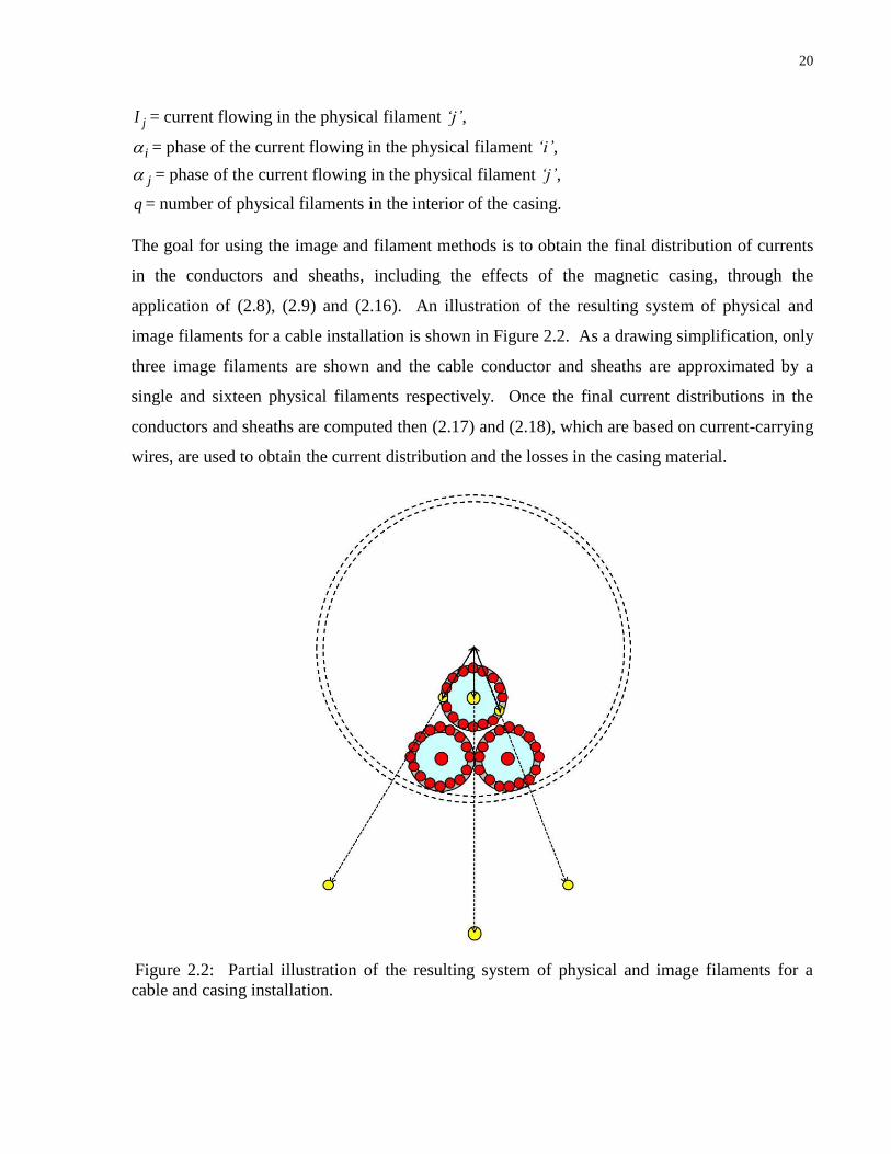
The goal for using the image and filament methods is to obtain the final distribution of currents
in the conductors and sheaths, including the effects of the magnetic casing, through the
application of (2.8), (2.9) and (2.16). An illustration of the resulting system of physical and
image filaments for a cable installation is shown in Figure 2.2. As a drawing simplification, only
three image filaments are shown and the cable conductor and sheaths are approximated by a
single and sixteen physical filaments respectively. Once the final current distributions in the
conductors and sheaths are computed then (2.17) and (2.18), which are based on current-carrying
wires, are used to obtain the current distribution and the losses in the casing material.
Figure 2.2: Partial illustration of the resulting system of physical and image filaments for a
cable and casing installation.

21
When only eddy currents exist in the sheaths, then from the experience of the author, it is enough
to approximate the images of the cable conductor and sheath filaments by a single filament
located at the image position of the center of the cable conductor and carrying a current related to
the given total current in the cable conductor according to (2.9). This is because, when only
eddy currents exist, the sheath image filaments do not carry significant currents that would alter
the losses in the system. This makes the equivalent image system easier to analyze. However,
when circulating currents are flowing in the sheaths, this approximation cannot be made, as
discussed next.
If the cable sheaths are multiple-point bonded in a three-phase circuit, the currents induced in
them will flow from one sheath to another. This circulating sheath current causes considerably
higher losses than the local eddy current losses. The final distribution of the currents in the cable
sheaths that are multiple-point bonded is calculated using the same filament and image methods
described in the previous sections, but with the imposed condition that the sum of all of the
sheath currents equals zero. In this case, it is important to use the images of all the original cable
conductor and sheath filaments, because the currents in the sheath image filaments are large
enough to alter the losses in the system.
2.4.2 Hysteresis loss
The second component of casing losses is called hysteresis loss and arises due to the
phenomenon of magnetic hysteresis [28]-[38]. This section discusses how to approximate
analytically the hysteresis loss for a system of cables inside a magnetic casing.
The B-H curve for a material experiencing magnetic hysteresis typically looks as shown in
Figure 2.3. The magnetic field intensity, H, fluctuates sinusoidally at a specific frequency f,
usually 50 or 60 Hz for power systems. So, one B-H loop is completed every 1/f seconds. The
area enclosed by this loop is equal to the heat dissipated per unit volume of the material due to
hysteresis. Multiplying the area by frequency, one obtains the dissipated power density.
The amplitude of the magnetic field intensity is non uniform in the casing. Its peak value affects
the loop shape and area, and it is generally very complicated to obtain precisely the area of the
loop from the peak of the magnetic field intensity. However, Steinmetz discovered in 1890 that

22
the loop area is related to the peak value of the magnetic flux density, B, through the following
empirical relationship, [21]:
loop area=h
g B (2.19)
where „g‟ and „h‟ are constants, „h‟ usually being around 1.6. Equation (2.19) holds for magnetic
flux density values up to 1.2-1.4T [40], which are not exceeded in typical casing installations.
Figure 2.3: B-H curve for a magnetic material [39].
The values of magnetic flux densities in a steel casing depend on the magnetic permeability of
the casing, which, in turn, depends on the peak value of the magnetic field intensity and the
hysteresis loop shape. The value of the magnetic intensity is also related to the magnetic flux
density. Time stepping is required to solve such a highly nonlinear problem. To simplify the
problem, an important approximation is made here: assume that the casing has a constant,
uniform “effective” magnetic permeability value. This assumption allows the system to be
solved analytically through Maxwell‟s equations with the use of phasors. The final analytical
solutions for the fields and power losses will have a closed form, which are faster to calculate
than by using the finite element or finite difference methods, and with comparable accuracy.

23
This value of constant permeability is calculated so that the resulting eddy current losses agree
with the actual nonlinear system. The calculation of this effective permeability is discussed in
the next section. Its validity is shown here as well.
With the approximation of constant permeability, the magnetic flux density distribution is
computed and the hysteresis loss is calculated from (2.19).
The magnetic flux inside the casing material, due to a single current filament in the interior
(superposition is used for multiple filaments), is given by:
0
1 1- ( ) sin( ( ))II
r n n
n
AB A K kr n n
r r
(2.20)
0
- ( )cos( ( ))IIn n
n
AB A k K kr n
r
(2.21)
Since 1k implies rB B , then:
BB (2.22)
0
( )cos( ( ))
h
hn n
n
A k K kr n
B (2.23)
Therefore, the hysteresis loop area becomes:
0
loop area ( )cos( ( ))
h
n n
n
g A k K kr n
(2.24)
The values of „g‟ and „h‟ are obtained for a specific steel material, given in [28], using curve
fitting, as shown in Appendix D, and are equal to:
5.913, 1.765g h (2.25)
2.4.3 Effective magnetic permeability of a steel casing
Steel casing has a non-constant magnetic permeability that depends on the strength of the
magnetic field excitation. The permeability of the steel casing is chosen to provide a good
approximation for the eddy current loss when compared with the actual nonlinear casing case.
The method presented here for calculating this effective permeability uses the ideas presented in
[20].

24
As shown in Section 2.4.1, the eddy current loss in the casing can be calculated using (2.18). It
can also be shown that, for a casing with constant permeability, the eddy current loss is
calculated by the following equation [20]:
2
0 ( ) 22
r pP f H b b
(2.26)
where 2( )H b is the average squared tangential magnetic field intensity at the casing inner
surface. The experimental B-H curve can be used to calculate r at different values of the
magnetic field intensity H. Because, in the casing the value of the radial magnetic field intensity,
rH , is much smaller than H , it can be assumed that H H (where 2 2
rH H H ). From
known values of r for different values of H , the casing eddy current loss is calculated for
different r . Using (2.26), one can then produce a plot of casing eddy current loss versus r .
On the other hand, a plot of the casing loss versus r can also be obtained by applying (2.18).
This plot and the previous plot can be drawn on the same axes, and because the two equations
must give the same casing loss for some specific value of r , the intersection of the two graphs
determines the value of r , as illustrated in Figure 2.4, for the system described in Section 2.5.2
and shown in Figure 2.9. This r is called the effective permeability. The effective permeability
value, in conjunction with equations (2.18) and (2.24), is used for the calculation of casing eddy
current and hysteresis losses.

25
Figure 2.4: Illustration of the effective permeability calculation
2.5 Results
Several tests were performed to determine the accuracy of the proposed analytical solution. The
results obtained using (2.9), (2.16), (2.18), and (2.24), were compared with the losses computed
using the “Eddy Current” solver of the commercial finite element program Maxwell by Ansoft
[41]. The tests were conducted in two phases. First, only eddy current losses in the casing were
considered, followed by the tests with both eddy current and hysteresis losses. The following
sections describe the tests and the obtained results.
2.5.1 Eddy current loss
This section presents test cases with constant value of the steel casing permeability. The purpose
of these test cases is to compare the eddy current loss calculation presented in this chapter
against results obtained by the Ansoft Maxwell (referred to from this point forward as Ansoft for
short).
The following cable systems were examined:
0 500 1000 15000
100
200
300
400
500
600
700
800
X: 1063
Y: 118.6
Relative permeability
Ca
sin
g e
dd
y c
urr
en
t lo
ss (
W/m
)Eq. (2.18)
Eq. (2.26)

26
1. Three sheathed cables at the center of the casing, sheaths single point bonded,
2. Three sheathed cables at the bottom of the casing, sheaths single point bonded,
3. Three sheathed cables at the bottom of the casing with circulating currents,
4. Two circuits, two sheathed cables per phase and circulating currents.
The four systems are illustrated in Figure 2.5, Figure 2.6, and Figure 2.7. Since the sheaths in
the first two systems are single-point bonded, only local sheath eddy currents are incurred,
whereas the sheaths in systems 3 and 4 are multiple-point bonded and thus sheath circulating
currents exist. System 4 contains two 3-phase circuits with two cables per phase. The first
circuit consists of the top six cables whereas the second circuit is comprised of the remaining
bottom six cables, and such that in each circuit the cables of the same phase are placed above
each other. For system 4, the sheaths of the cables within each circuit are connected together, but
sheaths of different circuits are not.
The cable conductors in systems 1-3 and the first circuit of system 4 are loaded with a balanced
current of 800A peak, while the bottom circuit of system 4 carries 1000A peak.
Figure 2.5: Cable system 1
Figure 2.6: Cable systems 2
and 3
Figure 2.7: Cable system 4
In all systems, the parameters assumed for the steel casing and cables are shown in Table 2.1.

27
Table 2.1: Parameters Common For All Tests
Frequency
(Hz)
Conductor
diameter (mm)
Sheath
thickness
(mm)
Diameter over the
insulation (mm)
Conductor, sheath
conductivity
(S/m)
60 26 2 48 74.46×10
Casing diameter
(mm)
Filament
diameter
(mm)
Casing
thickness
(mm)
Casing
conductivity
(S/m)
Casing relative
permeability
300 1 5 67.413×10 1500
The last value in the table, representing rather large relative permeability, is based on a magnetic
curve in [20] for a carbon-steel casing that has a maximum permeability of about 1750 with an
effective value of 1580.
The percentage difference in the casing eddy current losses computed by the proposed approach
and Ansoft is calculated as follows:
% 100*Analytical Method Ansoft
DifferenceAnsoft
(2.27)
In the following sections, “Error of Ansoft” refers to how close the numerical solution comes to
satisfying the electromagnetic equations that are being solved within the Ansoft program itself.
At the end of every iteration, the numerical solution is plugged back in to the field equations, and
the residual error is computed. If the residual error is zero, then the numerical solution is exact.
Ansoft also computes the total field energy and the field energy contributed to this by the
residual error. If the ratio of the residual error energy to the total field energy is less than a
preset value, then the iterations stop, and the simulation is assumed to have converged.
Otherwise, a finer mesh is generated, especially in the areas with large residual error, and the
simulation continues. The lower the final residual error and the finer the mesh, the more
accurate the solution, but the longer the simulation time will be. So, it is a compromise between
the speed and accuracy. Generally, in solving an eddy current problem with the interest of
calculating casing losses, a very small residual error is sought (less than 0.5% from the
experience of the author). The reason is that, in many cases, most of the residual error can be
concentrated in the casing region due to the very small skin depth of the eddy currents in the

28
casing. Therefore, a very fine mesh is needed there to obtain an accurate value for the casing
losses. The number of mesh triangles across the thickness of the casing is maintained to be at
least ten for all simulations.
The test cases results are given in Table 2.2.
Table 2.2: Eddy current losses computed with two different approaches
System Figure
Calculation
Time
(secs)
Accuracy
of Ansoft
Avg.
conductor
loss / cable
(W/m)
Avg.
sheath
loss
/cable
(W/m)
Total
casing
loss
(W/m)
Total loss
difference
3 sheathed
cables, center
of the casing
Proposed 2 14.81 3.05 0.68
-2.60%
Ansoft 46 0.18% 15.14 3.20 0.71
3 sheathed
cables, bottom
of the casing
Proposed 1.8 15.49 4.53 1.35
-0.52%
Ansoft 90 0.14% 15.45 4.62 1.45
3 sheathed
cables, bottom
of the casing
with
circulating
currents
Proposed 4.3 14.84 10.19 0.60
0.90%
Ansoft 40 0.29% 14.91 9.84 0.69
2 circuits, 2
cables /phase
with
circulating
currents *
Proposed 44 4.72 5.04 0.70
1.30%
Ansoft 193 0.31% 4.72 5.15 0.82
The results show an excellent agreement between the proposed method and the numerical
solution, and with a faster computation time. The results illustrate that the casing eddy current
losses are larger when the cables are in closer proximity to the casing wall, as expected due to
the pipe‟s exposure to a higher magnetic field. Furthermore, multiple-point bonding of the
sheaths gives rise to larger sheath losses but to lower casing losses. The higher sheath losses
arise from bigger circulating currents than the local eddy currents in single-point bonded sheaths.

29
The lower casing losses are due to the electromagnetic shielding effect of the sheath circulating
currents.
2.5.2 Eddy Current and Hysteresis Losses
This section presents test cases where eddy current and hysteresis losses of a nonlinear casing
are considered. The losses calculated by the proposed analytical method are compared with
those obtained using Ansoft. Ansoft is used to simulate both a case where the casing is set to
have a magnetic permeability equal to the “effective” permeability calculated for the analytical
method, and a case where the casing is set to have the experimental nonlinear magnetic curve.
Ansoft can solve directly for eddy current losses, but does not have its own method of
calculating hysteresis losses. So, to test the accuracy of the proposed method of calculating the
hysteresis losses using equation (2.24), which is based on a constant “effective” permeability, the
empirical equation (2.19) is invoked in Ansoft for both cases when the casing has constant
permeability and nonlinear magnetic curve.
The parameters shown in Table 2.3 were assumed for the steel casing and the cables.
Table 2.3: Parameters Common For All Tests
Frequency
(Hz)
Casing diameter
(mm)
Casing
thickness
(mm)
Casing
conductivity
(S/m)
Conductor, sheath
conductivity (S/m)
60 743 8.5 69×10 74.3×10
Conductor
diameter (mm)
Conductor
filament diameter
(mm)
Sheath
thickness
(mm)
Sheath filament
diameter (mm)
Cable diameter (up
to insulation) (mm)
43.8 10 3.75 8.76 106.1
Two cable configurations were considered in order to study the effect of proximity of the cables
to the casing wall and its effect on the accuracy of the effective permeability approximation and
the resulting cables and casing losses. The first case contains three cables arranged
symmetrically close to the center of the casing, as depicted in Figure 2.8. The second case has
the three cables configured non-symmetrically close to the casing wall, as shown in Figure 2.9.

30
The polar coordinates of the cable centers with respect to the casing center are given for the
aforementioned cases in Table 2.4 and Table 2.5, respectively. In both cases, the current loading
is equal to 1839A peak, and the cable sheaths are single-point bonded and therefore allowing for
only local sheath eddy currents.
Figure 2.8: symmetrical arrangement of
cables
Figure 2.9: asymmetrical arrangement of
cables
Table 2.4: Polar coordinates of cables in
Figure 2.8
Polar coordinate with
respect to casing center
Cable 1 (85 mm, 90.0o)
Cable 2 (85 mm, 210.0 o)
Cable 3 (85 mm, 330.0 o)
Table 2.5: Polar coordinates of cables in
Figure 2.9
Polar coordinate with
respect to casing center
Cable 1 (291.4 mm, -45.0o)
Cable 2 (280 mm, 160.0 o)
Cable 3 (290 mm, 200.0 o)
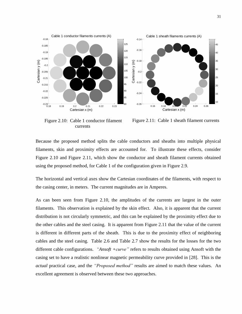
31
Figure 2.10: Cable 1 conductor filament
currents
Figure 2.11: Cable 1 sheath filament currents
Because the proposed method splits the cable conductors and sheaths into multiple physical
filaments, skin and proximity effects are accounted for. To illustrate these effects, consider
Figure 2.10 and Figure 2.11, which show the conductor and sheath filament currents obtained
using the proposed method, for Cable 1 of the configuration given in Figure 2.9.
The horizontal and vertical axes show the Cartesian coordinates of the filaments, with respect to
the casing center, in meters. The current magnitudes are in Amperes.
As can been seen from Figure 2.10, the amplitudes of the currents are largest in the outer
filaments. This observation is explained by the skin effect. Also, it is apparent that the current
distribution is not circularly symmetric, and this can be explained by the proximity effect due to
the other cables and the steel casing. It is apparent from Figure 2.11 that the value of the current
is different in different parts of the sheath. This is due to the proximity effect of neighboring
cables and the steel casing. Table 2.6 and Table 2.7 show the results for the losses for the two
different cable configurations. “Ansoft +curve” refers to results obtained using Ansoft with the
casing set to have a realistic nonlinear magnetic permeability curve provided in [28]. This is the
actual practical case, and the “Proposed method” results are aimed to match these values. An
excellent agreement is observed between these two approaches.
0.18 0.19 0.2 0.21 0.22 0.23-0.23
-0.225
-0.22
-0.215
-0.21
-0.205
-0.2
-0.195
-0.19
-0.185
-0.18
Cartesian x (m)
Ca
rte
sia
n y
(m
)Cable 1 conductor filaments currents (A)
80
85
90
95
100
105
110
115
120
125
0.16 0.18 0.2 0.22 0.24 0.26-0.26
-0.24
-0.22
-0.2
-0.18
-0.16
-0.14
Cartesian x (m)
Ca
rte
sia
n y
(m
)
Cable 1 sheath filaments currents (A)
10
15
20
25
30
35
40
45

32
To provide a comparison with another analytical method available in the literature, the same
problem is solved using Mekjian‟s approach [15], which neglects sheath losses and casing
hysteresis losses. Using the method of [15] the following results are obtained. Total conductor
loss = 110 W/m, total casing loss = 141 W/m. The corresponding total installation loss of
252W/m is 11% smaller than the actual loss of 282 W/m obtained using the “Ansoft +curve”.
Table 2.6: Losses for the system given in Figure 2.8
Proposed Ansoft Ansoft +curve
Casing relative permeability 850 850 non linear
curve in[16]
Calculation Time (s) 2 53 57
Error of Ansoft (%) N/A 0.48 0.09
Conductor loss (W/m) 102 104 103
Sheath loss (W/m) 32 32 31
Casing eddy loss (W/m) 6 7 6
Casing hysteresis loss (W/m) 3 3 2
Total loss (W/m) 143 145 142
Total loss difference (%) N/A -1.4 0.7

33
Table 2.7: Losses for the system given in Figure 2.9
Proposed Ansoft Ansoft +curve
Casing relative permeability 1063 1063 [16]
Calculation Time (s) 2 1920 2700
Error of Ansoft (%) N/A 0.52 0.24
Conductor loss (W/m) 102 103 103
Sheath loss (W/m) 19 18 19
Casing eddy loss (W/m) 118 120 120
Casing hysteresis loss (W/m) 42 42 40
Total loss (W/m) 281 283 282
Total loss difference (%) N/A -0.7 -0.4
Note that the value of relative permeability for the “Proposed” and “Ansoft” columns are
different in Table 2.6 and Table 2.7 for the two installations since it is computed using the
method discussed in Section 2.4.3 that depends on the cable geometry. The following
conclusions can be drawn from the presented results:
1) The total casing losses can be much greater than the total cable losses, as illustrated in
Table 2.7.
2) The total casing losses depend on the geometry of the cables inside. Cables that are
symmetrically arranged and far from the casing wall give rise to smaller losses than when
they are close to the pipe.
To analyze the effect of the assumed permeability on the loss computations with the proposed
method, a sensitivity analysis was conducted. Different constant permeabilities were assumed
and the corresponding installation losses were computed using the proposed method, for the
system consisting of three asymmetrically arranged cables close to the casing wall shown in
Figure 2.9. The results are given in Figure 2.12 - Figure 2.16. Note that the “Ansoft+curve”
values in these figures are identical to the results in Table 2.6, obtained using the actual
permeability curve in [16], and are shown for comparison with the proposed method solutions.
The following points can be inferred from the above graphs:

34
1) The “effective” permeability value determined by the method in Section 2.4.3, and equal
to 1063 in this case, provides losses that are in close agreement with the values given by
the most accurate method “Ansoft +curve”.
2) Although the total conductor loss applying Anosft program given in Figure 2.12 and
obtained using the proposed method do not coincide with the numerical value at any
chosen permeability, the proposed method computation does come very close to the
numerical calculation, especially considering that the values are rounded to the nearest
integer.
3) The conductor losses are almost independent of the chosen permeability value. This is
due to the small effect of the induced casing currents on the conductor current
distribution. A possible explanation is that the conductors carry large currents and are
shielded by the sheaths. Thus, the small current redistribution due to the proximity effect
of the casing gives rise to small changes in losses in comparison with the predominant
skin effect losses.
4) The sheath losses and casing hysteresis losses increase for larger casing permeabilities,
while the casing eddy current losses decrease for higher pipe permeabilities. It is difficult
to pinpoint the exact reasons for these trends, due to the complexity of the
electromagnetic interactions, and whether these variations are always true for any casing
installation. The casing eddy current losses increase with smaller skin depth, which is
smaller for larger permeabilities. However, a larger permeability could give rise to
smaller induced casing currents and, thus, possibly a lower eddy current loss. The
equations that pertain to the calculation of the losses are (2.9), (2.16), (2.18), (2.24).
These equations contain many installation-dependent constants, such as casing radius and
electrical conductivity, sheath and cable radii and conductivities etc. Another sensitivity
analysis could be performed to study the effects of these constants on the resulting trends
for sheath and casing losses versus assumed casing permeabilities. However, since an
exact understanding of these trends is not imperative for the objective of this thesis, the
sensitivity studies are left for possible future work.
5) Section 2.4.3 presents the method for computing the “effective” permeability by
matching casing eddy current losses computed with (2.18) and (2.26). However, Figure
2.14 shows that the determined value of “effective” permeability, 1063, does not
correspond to the exact intersection of the two graphs, although it brings them relatively

35
close. This is because (2.26), which uses the actual permeability curve, is derived based
on a constant casing permeability approximation, and thus the computed losses would be
different from those obtained using the numerical solution “Ansoft+curve”.
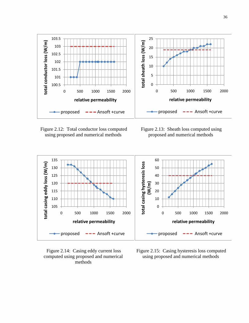
36
Figure 2.12: Total conductor loss computed
using proposed and numerical methods
Figure 2.13: Sheath loss computed using
proposed and numerical methods
Figure 2.14: Casing eddy current loss
computed using proposed and numerical
methods
Figure 2.15: Casing hysteresis loss computed
using proposed and numerical methods
100.5
101
101.5
102
102.5
103
103.5
0 500 1000 1500 2000tota
l co
nd
uct
or
loss
(W
/m)
relative permeability
proposed Ansoft +curve
0
5
10
15
20
25
0 500 1000 1500 2000
tota
l sh
eath
loss
(W
/m)
relative permeability
proposed Ansoft +curve
105
110
115
120
125
130
135
0 500 1000 1500 2000
tota
l cas
ing
edd
y lo
ss (
W/m
)
relative permeability
proposed Ansoft +curve
0
10
20
30
40
50
60
0 500 1000 1500 2000tota
l cas
ing
hys
tere
sis
loss
(W
/m)
relative permeability
proposed Ansoft +curve

37
Figure 2.16: Total installation loss computed
using proposed and numerical methods
2.6 Summary
This chapter presents an analytical solution for the calculation of losses in a steel casing caused
by an arbitrary arrangement of cables inside. The approximation uses the image and filament
methods as well as the concept of equivalent permeability. The results obtained with the
proposed approach agree very well with the solution obtained by application of the finite element
method to solve the same problem. The total loss difference of less than 3% is observed for all
tested cases. This closed form analytical solution is more insightful than its numerical
counterparts and could provide a basis for standardization of the computation of losses in a
system of cables inside a steel casing.
250
255
260
265
270
275
280
285
290
295
0 500 1000 1500 2000
tota
l lo
sse
s (W
/m)
relative permeability
proposed Ansoft +curve

38
Chapter 3 Configuration Optimization of Underground Cables for Best Ampacity
The main contribution of this chapter is:
A method for determining the optimal configuration of cables inside a duct bank and a
steel cylindrical casing resulting in the highest or the lowest total ampacity.
The method uses the following work in the literature:
1) Empirical and analytical equations from the standard IEC60287 relating the currents and
temperatures of cables in an arbitrary configuration,
2) Convex optimization routine for determining the total ampacity of cables in a given
configuration,
3) Genetic algorithm Vector Immune System (VIS) for solving combinatorial optimization
problems.
An important assumption is made in this chapter as follows:
The empirical equations from the IEC60287 standard for typically sized ducts are used
for a bigger sized cylindrical casing.
The material presented in this chapter is largely based on the paper accepted for publication in
the IEEE Transactions on Power Delivery [42].
3.1 Introduction
In large urban areas, cables are often laid in concrete duct banks to permit installation of several
circuits in a fairly confined space. Figure 3.1 shows an example of such an installation.

39
Figure 3.1: Example of cables located in a duct bank buried underground
In a duct bank installation with multiple available ducts, multiple cable configurations are
possible. Each configuration may lead to a different circuit ampacity, because the mutual
heating effect depends on cable locations as do the sheath and armour losses in each cable. The
configuration that leads to the maximum total ampacity is desirable to maximize the usage of a
limited duct bank space. On the other hand, the configuration with the smallest total ampacity is
desirable when cables have already been installed and information regarding which phases were
placed in which ducts is unknown, which happens quite often in practice when a large number of
cables are located in one duct bank. In this case, a worst-case scenario is of interest.
Recently, another important installation configuration has been gaining some attention—namely,
installing cables in steel or plastic casings. These are large casings containing a number of plastic
ducts as shown, for example, in Figure 3.2.

40
Figure 3.2: Cables inside a large casing
In addition to the issue of mutual heating and sheath/armour losses discussed above, this
installation may also result in very large hysteresis and eddy current losses in the magnetic
casing as discussed in Chapter 2. A question arises regarding how the cables should be placed in
the available ducts to minimize the losses in the magnetic casing and to maximize overall circuit
ratings.
A number of published works address the problem of cable ampacity calculations given cable
locations or configurations. There have been no published papers on location optimization
procedures that determine the best or worst cable configurations, from the total ampacity point of
view. The aim here is to present a procedure for finding the optimal cable configuration for
cables located in a duct bank or a casing.
The issue of finding the best configuration for a number of circuits is by its nature a
combinatorial optimization problem, due to the discrete solution space of possible
configurations. Reference [19] solves a problem of optimizing cables configuration with the
combined objectives of reducing the created magnetic fields and the current imbalance. This
problem is similar to the problem at hand from the point of view of optimizing the cable
configuration, but is different with regards to the objective of maximizing the total ampacity.

41
Therefore, the approach in [19], utilizing the Vector Immune System (VIS) algorithm, will be
used in this chapter to solve the problem of configuration optimization for best ampacity.
Section 3.2 provides an overview of a method for calculating the ampacity of a system of cables
placed in a fixed configuration. As a starting point, the method uses the Neher McGrath [1] and
IEC [2] standard equations, which have been verified in [43], and solves them using a convex
optimization algorithm that provides always convergent results. The convex optimization
algorithm finds the ampacity of a fixed cable configuration and, thus, serves as a single iteration
within an outer-level combinatorial optimization algorithm that attempts to find the best cable
configuration, from the point of view of the total system ampacity. The combinatorial
optimization procedure is based on the VIS algorithm and is briefly described in Section 3.3.
The proposed method is illustrated with two complex examples. One is a real-life duct bank
installation consisting of twelve cables and fifteen available ducts, comprising two different
circuits with two cables per phase and the second is a steel casing with six inner ducts in which
one 3-phase circuit is to be located. The results are presented in Section 3.4. Section 3.5
provides a summary.
3.2 Ampacity Calculation
This section presents an overview of a method for calculating the total ampacity of a group of
cables buried underground.
A typical power cable consists of a conductor, insulation, metallic sheath or screen, possible
armour bedding, armour, and external serving layers, as shown in Figure 3.3. The main sources
of heat generated by a cable are the Joule losses in the conductor, sheath/screen, armour, and
casing. In addition, some cables may produce substantial dielectric losses [5]. This heat is
dissipated through the various cable layers and the soil. The thermal resistances of the cable
layers and its surroundings influence the rate at which the heat is dissipated, and hence the rise of
the conductor temperature above the ambient temperature. This thermal interaction can be
represented, for the steady-state conditions, by a lump-parameter thermal circuit that
incorporates the thermal resistances of the cable layers and the soil, the Joule and dielectric
losses, and the ambient and conductor temperatures. The thermal circuit is then solved to obtain

42
the maximum conductor current, given the allowable insulation temperature. The solution for
the current, (A)I , is formulated in (3.1), with a comprehensive derivation given in [5].
0.5
max 1 2 3 4 int
1 1 2 1 2 3 4
(0.5 ( ))
(1 ) (1 )( )
dW T N T T TI
RT NR T NR T T
(3.1)
where:
1 = sheath loss factor, which is the ratio of the total sheath losses to the total conductor losses,
2 = armour loss factor, which is the ratio of the total armour losses to the total conductor losses,
R = conductor ac resistance ( / )m ,
dW = dielectric losses ( / )W m ,
N = number of load-carrying conductors in the cable,
1T = thermal resistance of the insulation ( / )Km W ,
2T = thermal resistance of the armour bedding ( / )Km W ,
3T = thermal resistance of the external serving ( / )Km W ,
4T = thermal resistance of the surrounding medium ( / )Km W ,
max max amb , max being the maximum allowable temperature of the cable conductor
and amb the ambient temperature,
int = conductor temperature reduction factor due to the heating from unequally loaded
neighboring cables.
The cable parameters depend on the material of each layer and its dimensions, and on the laying
conditions. The effect of mutual heating from neighboring cables is accounted for through int
if the cables are unequally loaded, or through a modified 4T , namely 4modT , if the cables are
equally loaded (i.e., are of the same construction and carry the same current). The cables can be
buried directly in the soil, in a thermal backfill, inside ducts within a duct bank, inside a large
cylindrical casing or in air. These different installation conditions are accounted for through
modifications of the surrounding thermal resistance, and an additional heat loss parameter for a
metallic casing installation. Methods for calculating the parameters for each type of installation
are given in Applendix E.

43
Figure 3.3: Underground cable construction
The calculation of the ampacities in a system of equally loaded cables can be done through the
direct use of (3.1) in conjunction with (E.9) for 4modT , for each cable. However, the
computation of the ampacities in a system of unequally loaded cables requires the incorporation
of the int , which is calculated in Section E.10 and gives rise to a set of equations that are not
trivial to solve, as discussed next.
It is evident from (3.1), (E.11) - (E.14) that in order to calculate the ampacity of a cable „i‟, the
currents of all the other cables must be known. However, these currents are not known a priori
because the objective is to compute the ampacities of all the cables in the system. The
application of (3.1) to every cable will result in a system of interrelated equations. In practice,
these equations are solved iteratively [5], [6], [11]. However, the iterative method is not always
convergent. A recently postulated alternative is to express these equations as an optimization
problem and then solve it to obtain the ampacities [9], [10]. This method is always convergent,
and is summarized next.

44
3.2.1 Convex Optimization Problem
Because the ampacity of a cable is the largest current that it can carry while not causing its
conductor temperature to rise above a specified maximum, the total ampacity of a group of
cables is the largest sum of the currents that do not cause any cable to overheat. Using (3.1) for
every cable, the resulting system of interrelated equations can be expressed, through algebraic
manipulations, as an optimization problem with an objective function of maximizing the sum of
all cable currents and with the constraints of having every cable conductor temperature below a
specified maximum. For balanced circuits, the phase currents must be equal and corresponding
equality constraints are added to the optimization problem. The resulting formulation for a
balanced system is given in (3.2), with a complete mathematical derivation detailed in [9].
1 2
2 2 21121 2
1 1 1
2 2 22211 2
2 2 2
2 2 21 21 2
1 1
1 1
1
n
nn
nn
i i ini
i i i i
Minimize I I I
ccsubject to I I I
d d d
ccI I I
d d d
c c cI I I I
d d d d
2
2 2 21 21 2
1
1 1
; 1,...,
n
n nn
n n n
ia ib ic
c cI I I
d d d
I I I i k
(3.2)
where k is the number of circuits composed of single core cables per phase, and ijc and id are
defined as follows:
1 2
1 1 2 1 2 3 4
(1 ) ln2
(1 ) (1 )( )
ijsj j j j j
ijij
i i i i i i i i i i i i
dN R
dc
R T N R T N R T T
, 1,...,
1,...,
i j
i n
j n
(3.2)
1
0.5 ( ) lnmax 1 2 3 4 2
(1 ) (1 )( )1 1 2 1 2 3 4
n
jj i
dijsW T N T T T N Wi di i i i i i j dj dij
di R T N R T N R T Ti i i i i i i i i i i i
, (3.3)
1,...,i n

45
This problem belongs to the class of continuous convex optimization problems [9]. Such type of
problems have a single local optimum, which is also the global optimum, and can be solved
effectively using the barrier method algorithm, which is briefly described in Appendix F and
detailed in [9].
So far, ampacities have been calculated for multiple cables placed at the specific known
positions, by solving a corresponding convex optimization problem. However, in some cases,
there are multiple available laying locations for the cables, and the engineer might be interested
in the optimal cable configuration, which would lead to the largest or the smallest possible total
ampacity. The need to find this optimal configuration leads to another optimization problem at a
different, outer level than the aforementioned convex optimization problem. The convex
optimization problem simply provides the total ampacities for a specific configuration and,
therefore, constitutes a single iteration in the outer-level combinatorial optimization problem that
seeks the best or worst configuration resulting in the optimal attainable total ampacity.
Considering all the possible cable configurations and calculating the total ampacity for each can
be a very time-consuming task. Instead, combinatorial optimization algorithms can be invoked
to solve this problem. The following section presents this outer-level combinatorial optimization
problem and provides an algorithm for solving it.
3.3 Cable Configuration Optimization
This section presents a method for configuring cables for the total ampacity. The method uses
the Vector Immune System (VIS) combinatorial optimization algorithm. Customization of this
algorithm to suit the problem being solved is presented in Appendix G.
Evolutionary algorithms such as the VIS are based on the survival of the fittest, where the traits
of only the fittest population are passed on from one generation to the next. This is achieved in
the VIS algorithm by structuring the operations into two nested loops, as illustrated by the
flowchart in Figure 3.4. In the inner loop, two operations are applied to the population, namely
cloning and mutation and clonal selection. The parent population from the previous iteration is
copied into clonesN clones, and each clone is mutated by random modifications. The mutation
operations are discussed in Appendix F. The parents and their mutated clones, also called
children, are each given a measure of fitness, according to their respective values of the objective

46
function. Among each parent and its children, the one with the best fitness is selected to become
the parent of the next generation, or inner iteration. This process ensures the fitness of the
population improves with every new generation. In the outer loop, the population undergoes
affinity, suppression, and random replacement. This is done by measuring the Euclidean
distance between the memory cells in the objective space, which in our case is the change in the
total system ampacity. All the memory cells, except the ones with distances below a preset
threshold, are suppressed, or deleted, and are replaced by randomly generated new ones. The
optimization algorithm ends when the numbers of outer and inner iterations reach their preset
limits, outN and inN . At this point, the parent solution with the best fitness is output as the final
solution. The greater the number of inner and outer iterations, the larger the probability that the
output solution is the sought optimal for the problem.
Figure 3.4: Flowchart illustrating the VIS algorithm [19].
Appendix G details some of the steps in the aforementioned algorithm and its customization to
suit the problem being solved here.

47
3.4 Numerical Examples
Two real-life installations for which the cable location plays an important role are examined
here. The first is a duct bank with several empty ducts and the second is a steel casing where the
losses in the steel casing are heavily dependent on the location of the cables. Cable dimensions
and parameters that are common to all cables used in the aforementioned two cases are given in
Table 3.1.
Table 3.1: Cable dimensions and current-independent parameters
Cable and Duct Bank Dimensions Cable and Ambient Parameters (current-
independent)
Cu conductor external
diameter (mm) 27.0 2 0
XLPE insulation external
diameter (mm) 49.8 N 1
Lead sheath external
diameter (mm) 53.8 dW ( / )W m (44 kV cable) 0
PE jacket external diameter
(mm) 59.4 1T ( / )Km W 0.341
PVC duct internal diameter
(mm) 170.1 2T ( / )Km W 0
Duct external diameter (mm) 199.0 3T ( / )Km W 0.095
Concrete duct bank
horizontal width (m) 1.6
o
max ( C) 90
o( C)amb 20
Duct bank vertical height
(m) 1.4
( / )soil Km W 1
( / )concrete Km W 0.6
3.4.1 Duct bank installation
We will analyze a 5x3 duct bank in which two circuits composed of two cables per phase each
are to be placed. The initial configuration of the cables is shown in Figure 3.5. The simulation
time on a Intel Pentium Dual Core 2 Ghz computer was about 20 minutes, and the final solutions
computed for the largest and the smallest ampacity cases are shown in Figure 3.6 and Figure 3.7,
respectively. The largest total ampacities per phase are 907A and 994A for circuits 1 and 2,

48
respectively, whereas the smallest total ampacities are 607A and 539A for circuits 1 and 2,
respectively.
Figure 3.5: Duct bank installation showing twelve cables in fifteen ducts and the corresponding
sequence representation
Figure 3.6: Configuration of cables for largest total ampacities per phase of 907A and 994A for
circuits 1 and 2, respectively

49
Figure 3.7: Configuration of cables for smallest total ampacity per phase of 607A and 539A for
circuits 1 and 2, respectively
Table 3.2: Cable ampacities, temperatures, sheath loss factors, ac resistances and thermal
resistances for the configuration in Figure 3.6
Cable Ampacity
(A)
Temperature
(˚C) 1
R ( / )m
4T
( / )Km W
1a 458 -118o
90.0 0.93 41.5 1.06
1a‟ 450 -122o
89.0 1.00 41.3 1.10
1b 496 0.45o
88.3 1.05 41.3 1.04
1b‟ 412 -0.54o
87.1 1.74 41.1 1.15
1c 443 117o
87.2 1.06 41.1 1.08
1c‟ 466 123o
89.7 0.88 41.4 1.09
2a 486 -119o
88.2 1.31 41.3 1.09
2a‟ 508 -121o
88.2 1.18 41.3 1.08
2b 518 5.04o
87.8 0.72 41.2 1.05
2b‟ 480 -5.44o
89.3 0.95 41.4 1.12
2c 530 123o
90.0 0.78 41.5 1.04
2c‟ 465 116o
88.5 1.16 41.3 1.11

50
Table 3.3: Cable ampacities, temperatures, sheath loss factors, ac resistances and thermal
resistances for the configuration in Figure 3.7
Cable Ampacity
(A)
Temperature
(˚C) 1 R ( / )m 4T ( / )Km W
1a 268 -123o
88.3 6.23 41.26 1.14
1a‟ 340 -117o
90.0 3.53 41.46 1.07
1b 297 10.5o
81.4 4.21 40.50 1.05
1b‟ 320 -9.72o
80.26 3.62 40.38 1.04
1c 337 116o
84.5 2.48 40.84 1.04
1c‟ 272 125o
81.2 4.25 40.48 1.09
2a 233 -121o
79.3 5.19 40.27 1.08
2a‟ 306 -119o
82.3 2.63 40.60 1.03
2b 306 2.63o
74.0 2.96 39.69 1.03
2b‟ 233 -3.46o
76.6 5.58 39.98 1.06
2c 289 113o
90.0 5.35 41.46 1.08
2c‟ 254 128o
87.9 7.22 41.23 1.12
The cable ampacities, conductor temperatures, sheath loss factors, ac resistances, and thermal
resistances of the surroundings are given in Table 3.2 and Table 3.3, corresponding to the
configurations in Figure 3.6 and Figure 3.7, respectively.
The simulation time for calculating the total ampacity of a single configuration is about 0.06 s.
Solving the combinatorial optimization problem through a brute force method by considering all
possible cable configurations and comparing their total ampacities would require 722 10
minutes (or 415 years) for 112 10 different permutations. Even if vertical symmetry is
considered, the simulation time would be halved and still be in the order of an unreasonable 207
years.
The size of the population and the number of clones are chosen to be equal to: 50popN and
5clonesN , respectively. There is no proof for the optimality of these choices, but rather they
are picked based on the experience of the author with solving this combinatorial optimization

51
problem. The number of the inner and outer loop iterations are: 12inN and 12outN .
Because the total number of iterations directly corresponds to the probability that the final
solution is identical to the sought optimal, these choices for the number of iterations are
important in determining the accuracy and simulation time of the proposed method. Generally,
the greater the number of iterations, the better the accuracy but the longer the simulation time
will be. The author has chosen the number of iterations such that for at least ten independent
simulations of the entire VIS procedure (clearing all variables and starting with a new random
population), the same final solution is obtained. This provides some level of confidence that the
final solution is the global, rather than a local, optimum for the problem. It is very difficult to
quantify the probability that the obtained solution is the global optimum, since there are multiple
possibilities for the installations, such as multiple circuits, multiple cables per phase, circulating
sheath currents, and the presence of steel casing. This probability quantification problem is left
as possible future work. Nevertheless, since the final solution is chosen only if is obtained in ten
independent simulations (and not iterations within the same simulation) of the entire VIS
program then it is reasonable to assume that the determined final solution is identical or close to
the global optimum. It is of course possible that the solution found is a local optimum and the
only sure way to ascertain that the algorithm has reached a global optimum is to compare the
results with a brute force approach. Such a comparison has been performed for a reasonably
sized practical case and is reported in Appendix H.
A sensitivity analysis was carried out to examine the effect of the number of iterations on the
accuracy and simulation time, with the results for this case presented in Figure 3.8. The total
number of iterations represent the product of inN and outN . While performing the analysis, the
author found that an equal change in the total number of iterations due to an increment of inN or
outN had almost the same effect on the accuracy and simulation time. Thus, only the total
number of iterations is shown. Due to the probabilistic nature of the applied algorithm, the data
points represent the total ampacity averaged over five simulations for a given total number of
iterations. The dashed horizontal line shows the final solution of the algorithm after simulating
for a very long time i.e. 30inN and 30outN . The results in Figure 3.8 provide some
justification for the author‟s selection of the number of iterations. As mentioned above, in order
to make a more precise assessment of the accuracy of the VIS final solution, the algorithm is

52
applied to a simpler duct bank installation, which can be optimized using the brute force method
within a reasonable amount of time, as presented in Appendix H. The VIS process results in a
configuration that is the true global optimal for the problem. Moreover, the VIS algorithm takes
a much shorter time to simulate than with the brute force approach. The agreement in the results
for this simpler case increases the confidence in the accuracy of the VIS search method.
Since for the installation in Figure 3.5 the largest total ampacities per phase are 907A and 994A
for circuits 1 and 2, respectively, whereas the smallest total ampacities are 607A and 539A for
the same circuits, this large difference in ampacity illustrates the importance of selecting proper
cable configuration. The best case scenario results in ampacities that are 49% and 84% larger
than the worst case scenario for circuits 1 and, 2 respectively. If knowledge of the installed
locations of the cable phases is unkown and the cables are loaded with the best case scenario
currents, the cables could overheat, which shortens the lifespan of the installation.
Figure 3.8: Total ampacity and simulation time for different number of iterations
0
300
600
900
1200
1500
5500
5550
5600
5650
5700
5750
1 4 9 16 25 36 49 64 81 100 144
Tim
e (
s)
Tota
l Am
pac
ity
(A)
Total Number of Iterations Total Ampacity
Time
5,703A

53
3.4.2 Cables in steel casing
The proposed method is also applied for an installation consisting of a single circuit inside a
large steel casing, with a single cable per phase and five available ducts. This installation is
illustrated in Figure 3.9, and its relevant parameters are given in Table 3.4. The same cables,
ducts and ambient conditions are used as in the duct bank installation, but the cable sheaths are
single-point bonded and, thus, no sheath circulating current losses are incurred (i.e. 1 0 ). The
cable currents cause eddy-current and hysteresis losses in the magnetic steel casing. These
losses are computed applying the analytical method outlined in Chapter 2. Different cable
configurations give rise to different casing losses and hence different cable ampacity. The
configuration resulting in the largest ampacity is shown in Figure 3.9 whereas the one giving rise
to the smallest ampacity is shown in Figure 3.10. Cable ampacities, temperatures and current
dependent parameters, pertaining to the configurations in Figure 3.9 and Figure 3.10 are
presented in Table 3.5 and Table 3.6, respectively. p is the ratio of the total casing losses to the
total cable conductor losses in the circuit. 41T is the thermal resistance outside of a cable but
inside the casing, whereas 42T is the thermal resistance outside the casing. The combinatorial
optimization algorithm parameters are as follows: 50popN , 5clonesN , 1inN and 1outN
.
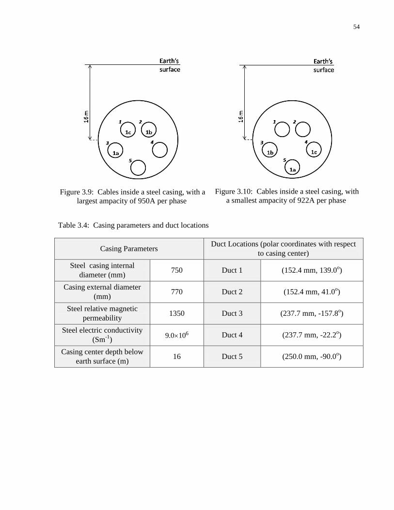
54
Figure 3.9: Cables inside a steel casing, with a
largest ampacity of 950A per phase
Figure 3.10: Cables inside a steel casing, with
a smallest ampacity of 922A per phase
Table 3.4: Casing parameters and duct locations
Casing Parameters Duct Locations (polar coordinates with respect
to casing center)
Steel casing internal
diameter (mm) 750 Duct 1 (152.4 mm, 139.0
o)
Casing external diameter
(mm) 770 Duct 2 (152.4 mm, 41.0
o)
Steel relative magnetic
permeability 1350 Duct 3 (237.7 mm, -157.8
o)
Steel electric conductivity
(Sm-1
)
69.0 10 Duct 4 (237.7 mm, -22.2o)
Casing center depth below
earth surface (m) 16 Duct 5 (250.0 mm, -90.0
o)

55
Table 3.5: Cable ampacities, temperatures, ac resistances, thermal resistances and total casing
loss ratio for the configuration in Figure 3.9
Cable Ampacity
(A)
Temperature
(˚C) R ( / )m 41 42;T T
( / )Km W p
1a 950.4 88.5 22.01 1.81; 0.70
0.69 1b 950.4 88.3 21.91 1.82; 0.70
1c 950.4 90.0 22.60 1.81; 0.70
Table 3.6: Cable ampacities, temperatures, ac resistances, thermal resistances and total casing
loss ratio for the configuration in Figure 3.10
Cable Ampacity
(A)
Temperature
(˚C) R ( / )m 41 42;T T
( / )Km W p
1a 921.9 88.9 21.96 1.79; 0.70
1.07 1b 921.9 88.9 21.96 1.79; 0.70
1c 921.9 90.0 22.44 1.79; 0.70
The results for the casing installation show that the largest ampacity of 950A is different but not
much bigger than the smallest value of 922A. This example illustrates that although the cables
are configured in almost the same way with respect to each other in Figures 3.9 and 3.10, they
are closer to the pipe in the latter and that increases the pipe losses and reduces the total
ampacity. For a larger pipe containing multiple circuits, the largest and smallest possible
ampacity can be drastically different.
3.4.3 Optimizing for total power
So far, the international standards and past work in the field of ampacity calculation have
addessed the problem of computing the maximum currents that circuits can carry without
overheating. However, for installations with multiple circuits having different voltages, the
computed maximum currents may not necessarily give rise to the largest power delivered, which
is important. Adjusting the presented procedure for optimizing the power is relatively simple,
and is achieved by modifying the objective function in (3.2) to represent the maximum total
power (being the sum of the products of current and voltage of the circuits). A numerical
example of the largest power cable configuration and a comparison with the biggest ampacity
configuration follow.

56
Figure 3.11 and Figure 3.12 respectively show the largest power and highest ampacity
configurations of two circuits inside a duct bank. Circuit 1 is comprised of 10kV cables, having
the specifications given in Table 3.1, while circuit 2 is made up of 110kV cables having the
dimensions and parameters as provided in Table 3.7. The cable ampacities and conductor
temperatures for the largest power and biggest ampacity configurations are given in Table 3.8.
Figure 3.11: Largest power configuration of 10kV and 110kV circuits
Figure 3.12: Largest ampacity configuration of 10kV and 110kV circuits
Table 3.7: 110kV cable dimensions and parameters

57
Cable Dimensions Cable Parameters (current-independent)
Cu conductor external
diameter (mm) 42.0 2 0
XLPE insulation external
diameter (mm) 88.0 N 1
Lead sheath external
diameter (mm) 101.0 dW ( / )W m 0
PE jacket external diameter
(mm) 108.0 1T ( / )Km W 0.412
2T ( / )Km W 0
3T ( / )Km W 0.066
o
max ( C) 90
Table 3.8: Cable ampacities and conductor temperatures for the largest power and biggest
ampacity configurations.
Largest power configuration Largest ampacity configuration
Cable Ampacity
(A)
Temperature
(˚C)
Ampacity
(A)
Temperature
(˚C)
1a 134.2 52.9 527.4 88.6
1b 134.2 52.0 527.4 90.0
1c 134.2 50.3 527.4 87.4
2a 685.2 83.3 646.7 87.3
2b 685.2 90.0 646.7 88.6
2c 685.2 84.9 646.7 90.0
These results show that optimizing for power rather than ampacity can lead to a higher total
power delivery and a cooler operation of the cables with lower cable ampacity values. Thus, it
may be beneficial to start analyzing cable systems from the point of view of power rather than
ampacity.
3.4.4 Configuration optimization insights
Since design engineers may not have access to the tools developed in this thesis, it would be very
helpful to develop a set of general conclusions or guidelines for the optimal placement of cables
with respect to ampacity. However, it is very difficult to devise definite rules for the optimal

58
allocation of cables because of the very large number of factors that can change from one
installation to another; to name a few: 1) the number of circuits, 2) the number of cables per
phase, 3) sheaths bonding arrangement, 4) depth of burial, 5) properties of soil, 6) distances
between ducts, 7) size of the pipe, 8)magnetic and electric properties of the pipe etc. The above
listed factors can have opposite effects on the cable placement. For example, cables that are
placed farther apart should be cooler, but the larger the separation the greater the sheath
circulating currents, and the associated heating losses, for multiple point bonded sheaths. Thus,
the optimal positioning would depend on the dominating effect, which may vary from one
installation to another. However, sensitivity analysis was carried out in order to determine
roughly some dominating effects, and the results are summarized below. However, for obtaining
the true optimal congiration, it is advised to use the tools developed in this thesis.
1. For cables in duct banks and casings, one should try to place them in a triangular
configuration (if possible with equal distances), since this reduces the circulating
current losses.
2. For cables in casings, the closer to the centre and more symmetrical the cables are
located, the lower steel losses will be.
3. Also, in cases when some circuits are more heavily loaded than the other, the more
heavily loaded cables should be placed closer to the centre of the casing.
4. For single point or cross bonded systems, in addition to placing the cables in a given
circuit in a triangular configuration, the cables should be separated as much as
possible.
5. For multiple point bonded systems, a triangular configuration is also preferable;
however, the two circuits should be placed below each other with opposite phase
sequence in each circuit. This is due to a magnetic field cancellation effect between
the two circuits that would reduce the eddy current losses in the conductors and
sheaths.
6. In both installations, the larger ampacity circuits should be placed towards the top of
the duct bank close to the earth‟s surface. This is due to a lower external thermal
resistance for cables located at a smaller depth.

59
3.5 Summary
This chapter presents a method for configuring the locations of any number of cables, with the
objective of obtaining either the largest or the smallest total ampacity, or power. The largest
ampacity configuration is useful when designing for a limited space, whereas the lowest
ampacity configuration is important when information regarding which phase occupies which
duct is unknown, and thus a worst-case scenario is considered. The optimal configuration is
obtained through a two-level optimization algorithm. At the outer level, a combinatorial
optimization algorithm that is based on the VIS algorithm explores the different possible
configurations. The performance of every configuration is evaluated according to its total
ampacity that is calculated using a convex optimization algorithm. The convex optimization
algorithm, which forms the inner level of the overall optimization algorithm, is based on the
barrier method. The proposed method is tested for a duct bank installation containing twelve
cables and fifteen ducts, comprising two circuits and two cables per phase, and for an installation
consisting of a single circuit in a large steel casing. The results obtained show that the proposed
method for the duct bank case is in the order of 610 times faster than using a brute force method
of trying all possible configurations. The steel casing example shows the effect of cable
configuration on casing losses and thus the ampacity of the circuit.
Optimizing for power rather ampacity, for installations with different-voltage circuits, shows that
it is possible to obtain a configuration with a higher total power delivery, cooler operation and
lower ampacities of the cables.
Finally, rough guidelines were developed, for specific types of installations, for configuring
cables leading to maximum total ampacity.

60
Chapter 4 Conclusions
4.1 Contributions and Remarks
The work presented in this thesis solves two problems in the field cable ampacity calculations.
One deals with calculation of the electromagnetic losses in steel casing installations containing
sheathed cables and the other concerns the determination of the optimal cable configurations in
the casings or duct banks. The main contributions are summarized as follows:
A new analytical method for approximating the electromagnetic losses in a system of
sheathed cables inside a magnetic steel casing. The method accounts for all of the
following:
arbitrary arrangement of the cables,
multiple circuits and/or multiple cables per phase,
multiple-bonding of sheaths and resulting circulating sheath currents,
nonlinear magnetic permeability of the casing and associated hysteresis losses.
A method for determining the optimal configuration of cables inside a duct bank and a
steel cylindrical casing resulting in the highest or the lowest total ampacity.
The results obtained using the proposed approach for calculating the electromagnetic losses in a
casing installation agree very well with the solutions obtained by application of the finite element
method to solve the same problem. The maximum loss difference of less than 3% is observed for
all tested cases. This closed form analytical solution is more insightful than its numerical
counterparts and could provide a basis for standardization of the computation of losses in a
system of cables inside a steel casing. Although the method presented in this thesis is applied for
cables and sheaths with circular cross-section, the solution process can be applied to cables and
sheaths of any shape, since they are decomposed into filaments.

61
The configuration optimization method presented in this work is tested for a duct bank
installation containing twelve cables and fifteen ducts, comprising two circuits and two cables
per phase, and for an installation consisting of a single circuit in a large steel casing. The results
obtained show that the proposed approach for the duct bank case is in the order of 610 times
faster than using a brute force method of trying all possible configurations. Furthermore, the
best case scenario results in ampacities that are 49% and 84% larger than the worst case scenario
for circuits 1 and 2, respectively. The steel casing example shows the effect of cable
configuration on casing losses and, thus, the ampacity of the circuit.
4.2 Suggested Future Work
The work presented in this thesis tackles the major obstacles arising in the calculation of losses
in a steel casing and in the configuration optimization of power cables. Relevant topics that were
not explored in this thesis but kept for future work are listed below:
1) Figures 2.10-2.14 in Section 2.5.2 show how various components of the losses vary with
the assumed value of casing permeability; some losses, such as casing hysteresis loss,
increase with increasing assumed permeability whereas others, such as casing eddy
current loss, decrease. It is not obvious whether each loss component exhibits the same
trend, for installations having different electrical conductivities and radii for the cable
conductor, sheath and casing. A sensitivity analysis can be conducted to study the effects
of these installation parameters on the losses trends.
2) The circuits considered for the examples in this thesis were balanced and carrying the
fundamental current component. The effects of phase current imbalances and current
harmonics on the casing losses can be investigated. Some insights regarding this study
follow: Since harmonics are of different frequencies, the law of superposition can be
applied to calculate the casing installation losses; the total losses are equal to the sum of
the losses at each current harmonic. The approach proposed in Chapter 2 can be used to
compute the losses at any frequency. Also, the phase current imbalances do not affect the
solution approach in Chapter 2, which provides freedom for the choice of the current for
each cable independently of other cables.

62
3) Installations with cables outside, but in close proximity to, a steel pipe (such as a water
pipe) have not been considered in this work. The effect of the current induced in the steel
pipe on the cable losses can be investigated. The method of images discussed in Chapter
2 for modeling the effect of the casing on the cables pertains to physical filaments inside
a casing and not outside. Electromagnetic analysis can be done to derive a similar
images-method for modeling physical filaments outside a steel pipe. For determining the
“effective” permeability, an equation that is conceptually similar to (2.26), which uses the
tangential magnetic field at the casing inner surface, can be derived in terms of the
magnetic field at the casing outer surface. This derivation is motivated by the fact that
the cable conductor currents are the source of the electromagnetic fields and will
therefore excite the outside surface of the pipe (with skin depth penetration).
4) Different cross-sectional shapes for the casing can be considered, such as square or
rectangular shapes. However, the presented equations using the method of images apply
for cylindrical casings. Therefore, different expressions have to be derived to account for
non-cylindrical steel casings.
5) For practicality purposes, tables or graphs providing losses for common casing and cable
sizes, and cable configurations can be prepared. Relatively simple equations based on
these results for the common cases can be also derived and added to the standards.

63
References
[1] J. H. Neher and M. H. McGrath, “The calculation of the temperature rise and load capability
of cable systems,” AIEE Transactions, Vol. 76, pt. III, pp. 752-772, Oct., 1957.
[2] Calculation of the continuous current rating of cables (100% load factor), IEC Standard
Publication 287, 2nd
ed., 1996.
[3] Carlos Garrido, Antonio F. Otero, and Jose Cidras, “Theoretical model to calculate steady-
state and transient ampacity and temperature in buried cables,” IEEE Transactions on Power
Delivery, Vol. 18, No. 3, July 2003.
[4] Sally M. Sellers and W. Z. Black, “Refinements to the Neher-McGrath model for calculating
the ampacity of underground cables,” IEEE Transactions on Power Delivery, Vol. 11, No. 1,
January 1996.
[5] George J. Anders, Rating of Electric Power Cables, IEEE Press / McGraw Hill, New York,
1997, pp. 190-193.
[6] “CYMCAP, Cable Ampacity Calculation,” CYME International T&D, Quebec, CA. [Online].
Available: http://www.cyme.com/software/cymcap/
[7] Francisco de Leon (2005). Calculation of underground cable ampacity, CYME International
T&D, Quebec, CA. [Online]. Available:
http://www.cyme.com/company/media/whitepapers/.
[8] Power Cable Ampacity Tables, IEEE Standard 835, 1994.
[9] W. Moutassem, “Optimization procedure for rating calculations of unequally loaded power
cables,” M.A.Sc. Thesis, Dept. ECE., University of Toronto, March 2007.
[10] G. J. Anders and W. Moutassam, “Barrier optimization algorithm applied to calculation of
optimal loading of dissimilar cables in one trench,” Proc. 2007 Jicable Conf.
[11] Julius Hegyi and Alex Y. Klestoff, “Current-carrying capability for industrial underground
cable installations,” IEEE Transactions on Industry Applications, Vol. 24, No. 1,
January/February 1988.
[12] Jurgen O. C. Kansog and Matthew T. Brown, “Ampacity calculations for mixed underground
cable systems in the same ductbank,” Proc. of the 1994 IEEE Power Engineering Society, pp.
535-543.
[13] Application of sheath-bonding methods for single conductor cables and the calculation of
induced voltages and currents in cable sheaths, ANSI/IEEE Standard 575, 1988.
[14] J. Poltz and E. Kuffel, “A simple and accurate evaluation of eddy-current loss in magnetic pipe
of a cable,” IEEE Transactions on Power Apparatus and Systems, Vol. PAS-104, No. 8,
August 1985, pp. 1951-1957.
[15] A. Mekjian, M. Sosnowski, and C. Katz, “A new method for calculating alternating current
losses in pipe-type cable systems,” IEEE Transactions on Power Apparatus and Systems, Vol.
PAS-101, No. 7, July 1982, pp. 1850-1858.

64
[16] Xiao-Bang Xu and Guanghao Liu, “Investigation of the magnetic field produced by
unbalanced phase current in an underground three-phase pipe-type cable,” Electric Power
Systems Research, pp. 153-160, 2002.
[17] D. Labridis and P. Dokopoulos, “Finite element computation of eddy current losses in
nonlinear ferromagnetic sheaths of three-phase power cables,” IEEE Transactions on Power
Delivery, Vol. 7, No. 3, July 1992, pp. 1060-1067.
[18] J. Kuang and S. A. Boggs, “Pipe-type cable losses for balanced and unbalanced currents,”
IEEE Transactions on Power Delivery, Vol. 17, No. 2, April 2002, pp. 313-317.
[19] A. Canova, F. Freschi, and M. Tartaglia, “Multiobjective optimization of parallel cable
layout,” IEEE Transactions on Magnetics, Vol. 43, No. 10, October 2007, pp. 3914-3920.
[20] A. Mekjian and M. Sosnowski, “Calculation of alternating current losses in steel pipes
containing power cables,” IEEE Transactions on Power Apparatus and Systems, Vol. PAS-
102, No. 2, February 1983, pp. 382-388.
[21] C. P. Steinmetz, “On the law of hysteresis,” Proceedings of the IEEE, Vol. 72, No. 2, February
1984, pp. 197-221.
[22] W. Moutassem and G. J. Anders, “Calculation of the eddy current and hysteresis losses in
sheathed cables inside a steel pipe,” IEEE Transactions on Power Delivery, accepted for
publication.
[23] R. Harrington, Time-harmonic electromagnetic fields. New York ; Toronto, McGraw-Hill,
1961.
[24] K. Kawasaki, M. Inami and T. Ishikawa, “Theoretical considerations on eddy current losses in
non-magnetic and magnetic pipes for power transmission systems,” Paper 80 SM54-7-0
presented at the IEEE 1980 Summer Power Meeting, Minneapolis, MN.
[25] M. Abramowitz and I. Stegun, Handbook of mathematical functions and formulas, graphs and
mathematical tables. National Bureau of Standards, Applied Mathematics Series-55, 1965
[26] J. Stammen, "Numerical computation of electromagnetic and thermal fields of high voltage
cable routes," Ph.D. dissertation, Dissertation Universität Duisburg, Shaker Verlag, 2001.
[27] J. D. Jackson, Classical Electrodynamics. John Willey & Sons, Inc., New York, 1962.
[28] Z. Cheng, N. Takahashi, Q. Hu, and C. Fan, “Hysteresis loss analysis based on Wh-Bm
function,” IEE Seminar Digests, Vol. 2002, No. 63, pp. 16, January 2002.
[29] G. Bertotti, “General properties of power losses in soft ferromagnetic materials,” IEEE
Transactions on Magnetics, Vol. 24, No. 1, January 1988, pp. 621-630.
[30] D. C. Jiles and D. L. Atherton, “Theory of ferromagnetic hysteresis,” Journal of Magnetism
and Magnetic Materials, Vol. 61, No. 1-2, 1986, pp. 48-60.
[31] I. D. Mayergoyz, Mathematical models of hysteresis and their applications, 1st ed..
Amsterdam ; Boston : Elsevier, 2003, pp. 377-468.
[32] G. Bertotti and I. D. Mayergoyz, The science of hysteresis, 3 v., Amsterdam ; Boston ; London
: Academic, 2006.

65
[33] A. A. Adly, I. D. Mayergoyz, R. D. Gomez, and E. R. Burke, “Computation of magnetic fields
in hysteretic media,” IEEE Transactions on Magnetics, Vol. 29, No. 6, November 1993, pp.
2380-2382.
[34] B. C. W. McGee and F. E. Vermeulen, “Power losses in steel pipe delivering very large
currents,” IEEE Transactions on Power Delivery, Vol. 17, No. 1, January 2002, pp. 25-32.
[35] D. C. Meeker, A. V. Filatov, and E. H. Maslen, “Effect of magnetic hysteresis on rotational
losses in heteropolar magnetic bearings,” IEEE Transactions on Magnetics, Vol. 40, No. 5,
September 2004, pp. 3302-3307.
[36] Z. Sigut and T. Zemcik, “Hysteresis loop analytical approximation,” Journal of Magnetism
and Magnetic Materials, Vol. 73, No. 2, 1988, pp. 193-198.
[37] C. Appino et al., “Power losses in thick steel laminations with hysteresis,” Journal of Applied
Physics, Vol. 79, No. 8, April 1996, pp. 4575-4577.
[38] F. Liorzou, B. Phelps, and D. L. Atherton, “Macroscopic models of magnetization,” IEEE
Transactions on Magnetics, Vol. 36, No. 2, March 2000, pp. 418-428.
[39] http://www.ndt-ed.org/EducationResources/CommunityCollege/MagParticle/Graphics/
BHCurve.gif
[40] F. J. G. Landgraf, M. Emura, and M. F. de Campos, “On the Steinmetz hysteresis law,”
Journal of Magnetism and Magnetic Materials 320, 2008, e531-e534, pp. 531-534.
[41] Ansoft, Maxwell-Electromagnetic field simulation for high-performance electromechanical
design, v12, [Online]. Available: http://www.ansoft.com/products/em/maxwell/
[42] W. Moutassem and G. J. Anders, “Configuration optimization of underground cables for best
ampacity,” IEEE Transactions on Power Delivery, accepted for publication.
[43] F. Aras, C. Oysu, and G. Yilmaz, “An assessment of the methods for calculating ampacity of
underground power cables,” Electric Power Components and Systems, Vol. 33, No. 12, pp.
1385- 1402, Dec. 2005.

66
Appendix A
Calculations of constants , , and C in equations (2.4)-(2.7)
The constants and are determined by imposing boundary conditions, which are the
continuity of the magnetic vector potential and of
between regions I and II.
The continuity of at the casing‟s inner surface (r = b) gives the following equation:
0 0
1 0
1cos( ( - )) - ln( ) ( ) cos( ( ))
2 2
n
n
n n n
n n
I IdB b n b C A K kb n
b n
(A.1)
Since this equation must be satisfied for any angle and since the cosine functions are
orthogonal for different „n‟, the following two equations can be derived from it:
0 1( ) for = 1, ,
2
n
n
n n n
I dB b A K kb n
b n
(A.2)
00 0- ln( ) ( )
2
Ib C A K kb
(A.3)
The continuity of
at the casing inner surface (r = b) gives the following equation:
-1 0 0
11 0
1 1 1cos( ( - )) - ( ) cos( ( ))
2 2
nn
n n nnn nr
n I IdnB b n A kK kb n
b n b
(A.4)
Again, since this equation must hold for any angle and since the cosine functions are
orthogonal for different „n‟, the following two equations can be derived from it:
-1 0
1
1 1( ) for = 1, ,
2
nn
n n nn
r
n I dnB b A kK kb n
b n
(A.5)
00 0
1 1- ( )
2 r
IA kK kb
b
(A.6)
The application of the boundary conditions resulted in four equations and four unknowns,
namely . Solving these four equations simultaneously results in the following
expressions for the unknown constants:

67
0 2
2 ( ) - ( )
n
rn
r n n
I dA
b n K kb kbK kb
(A.7)
0
2
( ) ( )1
2 ( ) - ( )
n
r n nn n
r n n
I n K kb kbK kbdB
n b n K kb kbK kb
(A.8)
0
0
0
-2 ( )
rI
Ab kK kb
(A.9)
0 0
0
( ) - ln( )
2 ( )
rI K kbC b
kbK kb
(A.10)

68
Appendix B
Derivation of the image current value
The expression derived for the magnetic vector potential in the interior of the casing is given by
(2.2) and is repeated here:
0 0
1
1cos( ( - )) - ln( )
2 2
n
n
I n
n
I IdA B r n r C
r n
(B.1)
This expression accounts for the magnetic vector potential contribution due to the physical
source-current filament and the contribution due to the induced current in the casing.
If the source current filament is located at the polar coordinates ( , )d in the interior of the
casing, and if the casing is replaced by an image filament located at ( , )d outside the casing,
the magnetic vector potential, in the region interior to the casing (i.e., 0 r b ), due to the
source and image filaments is given by:
0 0
1
0 0
1
1cos( ( - )) - ln( )
2 2
1cos( ( - )) - ln( )
2 2
n
I
n
n
n
I IdA n r
r n
I Irn d
d n
(B.2)
where I is the current carried by the image filament and is to be determined. There is flexibility
in choosing , ,d I , so that the above expression is equal to (B.1)given for the original system
of a source filament and a casing. If the values of , ,d I can be found to make these two
expressions equal, then the original and the equivalent systems will have the same
electromagnetic fields in the casing interior region. However, it is impossible to find values that
could achieve this. One can only achieve a best approximation. The reason for this is that, to
have the two equations match exactly, one would need to have 0 1 1
2
n
n
IB
d n
or all „n‟ and
0 ln2
IC d
. nB as been determined previously to be a complex number that is given by a
quotient of two polynomials in „n‟. Although I is a complex number, there is no way to
represent exactly a quotient of two polynomials in „n‟ by a quotient of an exponential function

69
and the function „n‟, i.e. 1 1
n
d n
. This is not possible for every integer 1, ,n . An
important assumption is made here: the values of , ,d I will be chosen so that the magnetic
vector potentials for the original system, (B.1), and the equivalent “image” system, (B.2), are
approximately matched at the casing inner surface. This assumption is achieved by equating the
magnetic vector potentials at the point on the casing inner surface that is closest to the filament—
i.e., at ( , )b —and, thus, the condition simplifies to (B.3) and (B.4).
1
0
1
1
2
n
n
n
n
n
B b
Ib
d n
(B.3)
2bd
d (B.4)
Equations (B.3) and (B.4) include only the contribution of the magnetic potential terms that fall
under the summation, because they capture the angular variation of the magnetic potential.
To test the above approximation for the accuracy of the electromagnetic fields in the interior of
the casing, consider the system shown in Figure B.1.

70
Figure B.1: Three filaments inside a steel casing
Table B.1 : Polar coordinates of
filaments in Figure B.1
Polar coordinate w.r.t.
casing center
Filament 1 (202 mm, -29.7o)
Filament 2 (249 mm, 149.8 o)
Filament 3 (221 mm, 213.0 o)
The system consists of a steel casing containing three filaments carrying a balanced current of
1554 A peak. The relevant system parameters are as in Table 2.3, except for a casing
conductivity of 6 -16.41×10 Sm and a casing permeability of 700. The filaments are located as
given in Table B.1. The system is solved using the following approaches: 1) Analytically for
the original system using (B.1), 2) Analytically for the equivalent “images system” using (B.2)
and the proposed approximation given by (B.3) and (B.4), 3) Analytically for the equivalent
“images system” using Mekjian‟s images approximation (from Section 2.2.2). The magnetic
vector potential at the inner surface of the casing using the three different methods is plotted in
Figure B.2.
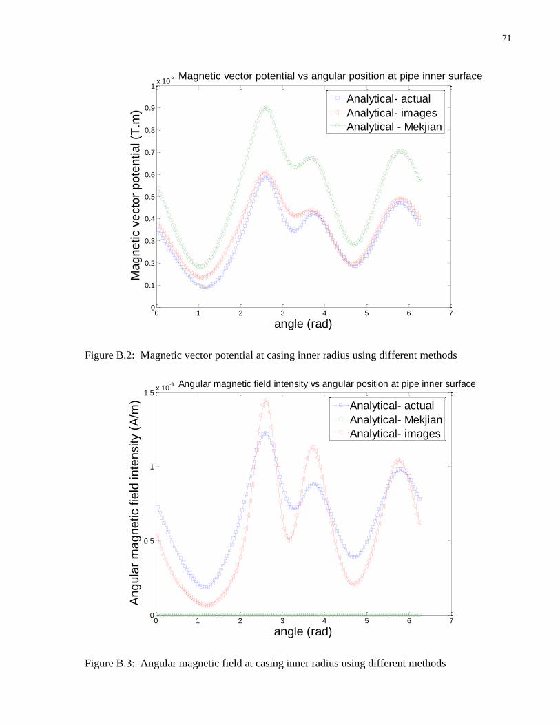
71
Figure B.2: Magnetic vector potential at casing inner radius using different methods
Figure B.3: Angular magnetic field at casing inner radius using different methods
0 1 2 3 4 5 6 70
0.1
0.2
0.3
0.4
0.5
0.6
0.7
0.8
0.9
1x 10
-3
angle (rad)
Ma
gn
etic v
ecto
r p
ote
ntia
l (T
.m)
Magnetic vector potential vs angular position at pipe inner surface
Analytical- actual
Analytical- images
Analytical - Mekjian
0 1 2 3 4 5 6 70
0.5
1
1.5x 10
-3
angle (rad)
An
gu
lar
ma
gn
etic f
ield
in
ten
sity (
A/m
)
Angular magnetic field intensity vs angular position at pipe inner surface
Analytical- actual
Analytical- Mekjian
Analytical- images

72
Figure B.4: Radial magnetic field at casing inner radius using different methods
It can be observed that the magnetic vector potential for the image method has good agreement
with that for the actual original system, whereas agreement is not so good for the magnetic
vector potential obtained with the Mekjian‟s method.
Figures B.3 and B.4 show the angular and radial magnetic field intensities at the inner surface of
the casing for the three different methods. Note that the angular magnetic field in Figure B.3 for
the Mekjian‟s method is zero. It can be seen that the proposed approximation gives rise to the
angular and radial magnetic fields that are in better agreement with the analytical solution of the
original system than given by the Mekjian‟s approximation.
0 1 2 3 4 5 6 70
0.2
0.4
0.6
0.8
1
1.2x 10
-3
angle (rad)
Ra
dia
l m
ag
ne
tic f
ield
in
ten
sity (
A/m
)
Radial magnetic field intensity vs angular position at pipe inner surface
Analytical- actual
Analytical- Mekjian
Analytical- images

73
Appendix C
Derivation of the general power loss with the geometry factor Yn
For a single conductor, the magnetic vector potential inside the casing is as follows:
1
0
( ) cos( ( ))II n n
n
A A K kr n
(C.1)
where 0 1 1 2
2 ( ) - ( )
n
rn
r n n
I dA
b n K kb kbK kb
, and the conductor is located at 1 1( , )d and is
carrying current 1I .
For multiple „m‟ conductors, the magnetic vector potential is:
1 0
( ) cos( ( ))i
m
II n n i
i n
A A K kr n
(C.2)
where 0 2
2 ( ) - ( )i
n
i i rn
r n n
I dA
b n K kb kbK kb
, and the conductor is located at ( , )i id and is
carrying current iI . The resulting current density inside the casing and the associated power loss
are given by (C.3) and (C.4) respectively.
0
- - ( )cos( ( - ))iz p II p n n i
n
J j A j A K kr n
(C.3)
2 22 22
0 0
1 1
2 2p II
p b b
P J rd dr A rd dr
(C.4)
Equation (C.2) can be written in the following form by breaking up complex numbers into their
real and imaginary components:
1 0
Re( ( )) cos( ( )) Im( ( )) sin( ( ))i i
m
II n n i n n i
i n
A A K kr n A K kr n
(C.5)
Calculating
(C.6)
i i
2 2m m
2
n n i n n i
i 1 n 0 i 1 n 0
Re(A K (k )) cos(n( )) Im(A K (k )) sin(n( ))
IIA r r

74
Since the expression for the current density as given by (C.3) leads to the integration of (C.6)
with respect to then only the following terms will be non-zero:
2 20 1 12
0 0
0 1 1
Re( ( )) Re( ( ))cos( ( ))cos( ( ))
Im( ( )) Re( ( ))sin( ( ))sin( ( ))
i j
i j
m m
n n n n i j
n i j
II m m
n n n n i j
n i j
A K kr A K kr n n
A d d
A K kr A K kr n n
(C.7)
Further expansion shows that only the following terms would remain under integration:
2 2
20 1 12
2 20
0 1 1
Re( ( )) Re( ( )) cos ( )cos( )cos( ) sin ( )sin( )sin( )
Im( ( )) Im( ( )) sin ( )cos( )cos( ) cos ( )sin( )sin( )
i j
i j
m m
n n n n i j i j
n i j
II m m
n n n n i j i j
n i j
A K kr A K kr n n n n n n
A d
A K kr A K kr n n n n n n
2
0
d
(C.8)
Performing the integration with respect to results in the following:
20 1 12
0
0 1 1
Re( ( )) Re( ( )) cos( ( ))
Im( ( )) Im( ( )) cos( ( ))
i j
i j
m m
n n n n i j
n i j
II m m
n n n n i j
n i j
A K kr A K kr n
A d
A K kr A K kr n
(C.9)
Define ( )in nA K kr as follows:
0( ) 2i
n
in n i i n n n n
dA K kr I D E
b
(C.10)
2
( ) ( )
rn
r n n
Dn K kb kbK kb
(C.11)
2
( ) ( )
rn
r n nn K kb kbK kb
(C.12)
( )n nE K kr
(C.13)
( )n nK kr
(C.14)
Taking the real and imaginary parts of ( )in nA K kr results in the following:
0Re ( ) cos( )2i
n
in n i n n i n n
dA K kr I E D
b
(C.15)

75
0Im ( ) sin( )2i
n
in n i n n i n n
dA K kr I E D
b
(C.16)
Substituting (C.15) and (C.16) in (C.9) gives:
2
2 22 02
0 1 10
cos( ( )) [cos( )2
cos( ) sin( )sin( )]
nn
jim mi j i j n n i n n
II
n i j
j n n i n n j n n
ddn I I E D
A d b b
(C.17)
222 2 20
0 1 10
cos( )cos( ( ))2
nnm mji
II i j n n i j i j
n i j
ddA d I I E D n
b b
(C.18)
Thus, the following may be derived:
32
2 2 2 21
21
4 2
n p
n
np p p
ZP Y
b n Z n Z
(C.19)
22 2
21 1
2 cos( ( - ))cos( - )
nnk k ki ji
n i i j i j i j
i j i i
d ddY I I I n
b b
(C.20)

76
Appendix D
Calculation of ‘g’ and ‘h’ in equation (2.25) for hysteresis loss
The values of „g‟ and „h‟ for the hysteresis loop area relation given in (2.19) can be obtained by
analyzing the hysteresis loss experimental data given for a specific steel material. The steel
material used in this thesis is analyzed in [28], where the following table is provided showing the
hysteresis loss values for different magnetic flux densities:
Table D.1: Hysteresis loss of steel in [28] at different values of magnetic flux density
B (T) Hysteresis
Loss (W/kg) B (T)
Hysteresis
Loss (W/kg)
0.049 0.02 1.45 11.86
0.101 0.11 1.5 12.8
0.15 0.24 1.55 13.77
0.2 0.41 1.6 14.68
0.299 0.82 1.639 15.28
0.399 1.32 1.67 15.73
0.499 1.88 1.701 16.22
0.601 2.51 1.729 16.84
0.7 3.21 1.76 17.32
0.801 3.98 1.781 17.51
0.899 4.82 1.8 17.57
1.001 5.77 1.83 17.75
1.099 6.81 1.85 17.72
1.2 8.01 1.875 17.82
1.3 9.39 1.9 17.85
1.401 10.99
Since Steinmetz‟s law is accurate for magnetic flux density values up to 1.4 T [40], a plot of
hysteresis loss versus „B‟ is made for „B‟ values up to 1.4 T. This plot is shown in the figure
below:
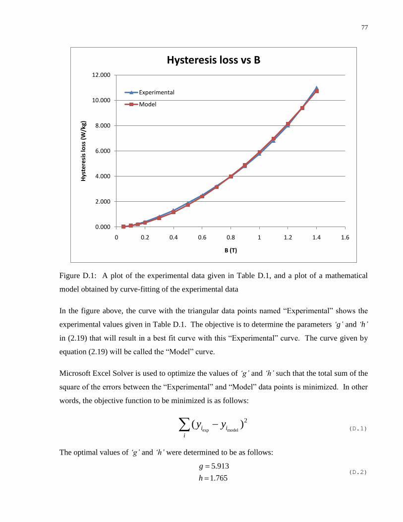
77
Figure D.1: A plot of the experimental data given in Table D.1, and a plot of a mathematical
model obtained by curve-fitting of the experimental data
In the figure above, the curve with the triangular data points named “Experimental” shows the
experimental values given in Table D.1. The objective is to determine the parameters „g‟ and „h‟
in (2.19) that will result in a best fit curve with this “Experimental” curve. The curve given by
equation (2.19) will be called the “Model” curve.
Microsoft Excel Solver is used to optimize the values of „g‟ and „h‟ such that the total sum of the
square of the errors between the “Experimental” and “Model” data points is minimized. In other
words, the objective function to be minimized is as follows:
exp model
2( )i i
i
y y (D.1)
The optimal values of „g‟ and „h‟ were determined to be as follows:
5.913
1.765
g
h
(D.2)
0.000
2.000
4.000
6.000
8.000
10.000
12.000
0 0.2 0.4 0.6 0.8 1 1.2 1.4 1.6
Hys
tere
sis
loss
(W
/kg)
B (T)
Hysteresis loss vs B
Experimental
Model
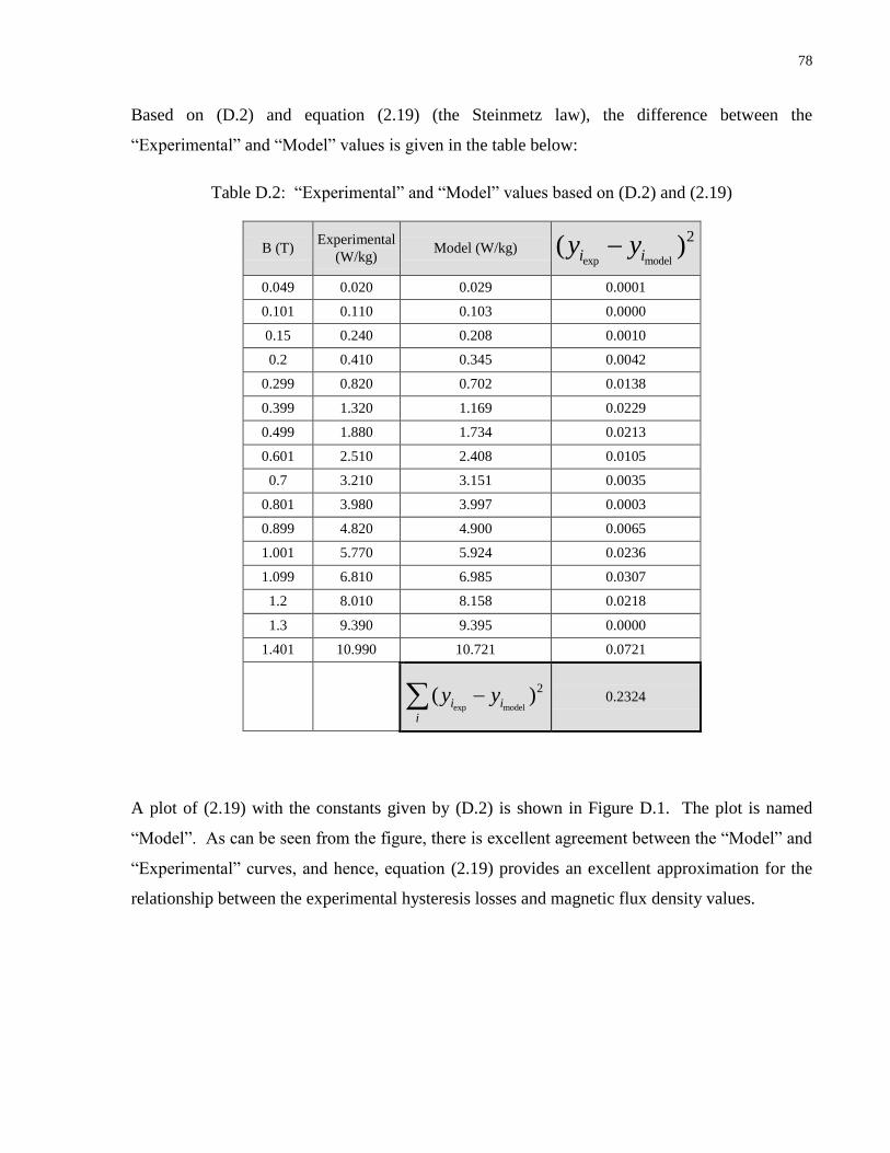
78
Based on (D.2) and equation (2.19) (the Steinmetz law), the difference between the
“Experimental” and “Model” values is given in the table below:
Table D.2: “Experimental” and “Model” values based on (D.2) and (2.19)
B (T) Experimental
(W/kg) Model (W/kg)
exp model
2( )i iy y
0.049 0.020 0.029 0.0001
0.101 0.110 0.103 0.0000
0.15 0.240 0.208 0.0010
0.2 0.410 0.345 0.0042
0.299 0.820 0.702 0.0138
0.399 1.320 1.169 0.0229
0.499 1.880 1.734 0.0213
0.601 2.510 2.408 0.0105
0.7 3.210 3.151 0.0035
0.801 3.980 3.997 0.0003
0.899 4.820 4.900 0.0065
1.001 5.770 5.924 0.0236
1.099 6.810 6.985 0.0307
1.2 8.010 8.158 0.0218
1.3 9.390 9.395 0.0000
1.401 10.990 10.721 0.0721
exp model
2( )i i
i
y y
0.2324
A plot of (2.19) with the constants given by (D.2) is shown in Figure D.1. The plot is named
“Model”. As can be seen from the figure, there is excellent agreement between the “Model” and
“Experimental” curves, and hence, equation (2.19) provides an excellent approximation for the
relationship between the experimental hysteresis losses and magnetic flux density values.

79
Appendix E
Calculation of parameters for cable ampacity computation
This appendix summarizes equations for the calculation of cable parameters that are relevant in
the ampacity computation. The equations are extracted from [5].
E.1 Sheath Loss Factor, 1 :
The sheath losses in cables can be computed using an analytical approach that is based on self
and mutual inductance equations of the cable conductors and sheaths. Cable installations can be
comprised of single or multiple circuits with single or multiple cables per phase. The case of
multiple cables per phase is more complicated to analyze. Thus, the calculation of the sheath
loss factor of a cable is described within Section E.13 that presents a method for analyzing the
calculation of sheath loss factors and conductor current distribution in circuits with multiple
cables per phase. Sheath loss computation for single cables per phase is considered as a special
and simple case of the multiple cables per phase analysis.
E.2 Armor Loss Factor, 2 :
Cables containing a magnetic conductive armor incur losses due to the induced currents in the
armor. The cables considered in this thesis will not contain an armor layer and thus the armor
loss factor will be equal to zero. A complete description of the armor losses can be found in [5].
E.3 Conductor AC resistance, R:
The current in the conductor distributes itself such that it flows close to the conductor outer
surface. This phenomenon is known as the skin effect. Skin effect causes an increase in the
resistance of the conductor. The resistance of the conductor including the skin effect is the ac
resistance of the conductor. The effect of neighboring cables currents on the conductor‟s current
distribution, also known as the proximity effect, is neglected since it is negligible for sheathed
cables. The calculation of the ac resistance of a conductor is carried out according to the
following empirical approximation:

80
7
,
8 60 1 10 ss
dc c
kx
R
(E.1)
4
4192 0.8
ss
s
xy
x
(E.2)
, 1 20cdc c c c
c
RA
(E.3)
, , 1ac c dc c sR R y (E.4)
where sk is an empirical constant that accounts for conductor stranding, , ( / )dc cR m is the dc
resistance, ( )c m is the electrical resistivity, 2( )cA m is the cross-sectional area, 1( )c K is
the temperature coefficient, o( )c C is the temperature, and , ( / )ac cR m is the ac resistance.
E.4 Dielectric losses, dW :
The insulation acts as a dielectric between the cable conductor and metallic sheath/armor. This
dielectric incurs significant dielectric losses for high voltage levels. The voltage levels of the
cables considered in this thesis are relatively low and the dielectric losses can be neglected. The
reader is referred to [5] for a comprehensive review the calculation methods of cable dielectric
losses.
E.5 Thermal Resistance of Insulation, 1T :
The thermal resistance of a cylindrical insulation covering the conductor, 1( / )T Km W , can be
calculated as follows:
1 log 1 22
i i
c
tT
d
(E.5)
where:
i = thermal resistivity of the insulation material
( / )Km W ,
it = thickness of the insulation ( )m ,
cd = outer diameter of the conductor shield ( )m .

81
E.6 Thermal Resistance of Armor Bedding, 2T :
The thermal resistance of a cylindrical armor bedding covering the sheath, 2( / )T Km W , can be
calculated as follows:
2 log 1 22
a a
s
tT
d
(E.6)
where:
a = thermal resistivity of the armor bedding material ( / )Km W ,
at = thickness of the armor bedding ( )m ,
sd = outer diameter of the sheath ( )m .
E.7 Thermal Resistance of External Serving, 3T :
The thermal resistance of a cylindrical external serving covering the armor, 3( / )T Km W , can be
calculated as follows:
3 log 1 22
j j
a
tT
d
(E.7)
where:
j = thermal resistivity of the jacket or external serving material ( / )Km W ,
jt = thickness of the serving ( )m ,
ad = outer diameter of the armor ( )m .
E.8 Thermal Resistance of Surroundings, 4T :
For a single cable buried underground the thermal resistance of the surrounding, 4( / )T Km W ,
can be calculated as follows:
2
4
2 2log 1
2
s
e e
L LT
d d
(E.8)
where:
s = thermal resistivity of the surrounding soil ( / )Km W ,
L = depth of cable center below the earth‟s surface ( )m ,

82
ed = outer diameter of the cable ( )m .
E.9 Modified Thermal Resistance of Surroundings for Equally
Loaded Cables, 4modT :
If all the installation cables are equally loaded, then the principle of superposition is used to
account for the mutual heating effect between the cables through a modification of the external
thermal resistance. The principle of superposition uses some simplifying assumptions, namely:
1) soil resistivity is constant everywhere and does not change with the heat field, 2) the earth‟s
surface is an isotherm, and 3) the cables act as line sources and do not distort the heat field from
other cables. The third assumption is approximately valid if the cables are axially spaced not
less than two cable diameters, which is the case for the duct banks and casing installations
analyzed in this thesis. The modified resistance, 4modT ( / )Km W , is calculated as follows:
4mod
4log
2
s
e
L FT
d
(E.9)
where F is a factor that depends on the geometry of the cables. The value of this factor for a
cable „i‟ in a system of n cables is obtained from:
1
nij
ijjj i
dF
d
(E.10)
where ijd is the distance between centers of cable „i‟ and cable „j‟, ijd is the distance between
center of cable „i‟ and the image, with respect to the earth‟s surface, of cable „j‟. These distances
are illustrated in Figure E.1.

83
Figure E.1: Illustration of the distances between cables and their images for the calculation of
the geometric factor in (E.10)
E.10 Temperature Reduction Factor for Unequally Loaded
Cables, int :
If there are multiple circuits in the installation with unequally loaded cables, the mutual heating
effect is accounted for through a temperature reduction factor, int . The principle of
superposition is used with the same assumption as in Section E.9. Calculating int for the
ampacity equation of the cable of interest „i‟ is obtained by summing up the heat influences of all
neighboring cables, as given by (E.11). The heat influence by cable „j‟ on cable „i‟, ij , is
calculated using (E.12) by multiplying the heat produced by the cable „j‟, jW , and the mutual
thermal resistance ijT between cables „j‟ and „i‟. jW is the sum of the Joule and dielectric losses
of cable „j‟, as expressed in (E.13). ijT depends on the distance between the two cables and their
depth below the earth‟s surface and is calculated using (E.14).

84
int
1
n
ij
jj i
(E.11)
ij j ijW T (E.12)
2
1 2[ (1 ) ]j j j j j j djW N I R W (E.13)
ln2
ijsij
ij
dT
d
(E.14)
In (E.11), n is the total number of cables in the system. For cable „j‟, jI is its conductor
current, jR is its ac resistance ( /m) , 1 j and 2 j are its sheath and armour loss factors,
respectively, N is the number of conductors in the cable, j is its loss factor, and ( / )djW W m is
its dielectric loss. Calculation of the mutual thermal resistance becomes somewhat more
involved when the cables are located in a duct bank, backfill or a large casing [5].
E.11 Cables inside a duct bank
It is very common to have cables inside ducts within a duct bank, especially when the available
space is scarce. This allows for the installation of multiple circuits in the same confined area as
shown in Figure 3.1. The presence of cables inside the ducts within the duct bank alters the
calculation of the thermal resistance of the surroundings, as seen by each cable.
Each cable is located inside a duct, with all the ducts affixed within a thermally favorable
material. The heat generated inside the cable must be dissipated through the medium (air or
fluid) between the cable and the inner surface of the duct, then through the duct wall, into the
duct bank thermal material and finally through the soil. Thus, the total external thermal
resistance of the surroundings as seen by each cable is the sum of the thermal resistances due to
the medium between the cable and duct, 4dT , the duct wall material, 4dT , and the duct bank
material and the soil, 4dT :
4 4d 4d 4dT T T T (E.15)
The calculation of each thermal resistance component is discussed next.
The thermal resistance of the medium between the cable exterior and the inner duct wall is
calculated using an empirical relationship that assumes the cable is located at the center of the

85
duct [5]. This thesis considers only cases where the medium is air and, thus, the equation for air
is presented here, with [5] providing equations for other media.
.4d 3
m e
UT
1 0 1 V Y d 10
(E.16)
where U, V, Y are empirical constants that pertain to the type of duct and medium and ( )o
m C is
the average temperature of the air filling the duct.
The thermal resistance of the cylindrical duct wall, 4( / )T Km W , is calculated using the
following analytical relationship:
4 log2
d did
de
dT
d
(E.17)
where:
d = thermal resistivity of the duct material ( / )Km W ,
did = inner diameter of the duct ( )m ,
ded = external diameter of the duct ( )m .
The thermal resistance of the surrounding duct bank material, 4( / )T Km W , is calculated using
(E.8) that pertains to directly buried cables, but with the replacement of the soil with the duct
bank material, and added a correction for the surrounding soil. The resulting equation is (E.18).
2 2
4
2 2 ( )log 1 log 1
2 2
b b b s b b bd
de de b b
L L L LT
d d r r
(E.18)
exp log log
2bybx bx bx
bby by bx
LL L L1 4r 1
2 L L L 2
(E.19)
where:
b = thermal resistivity of the duct bank material (usually less than that of soil) ( / )Km W ,
bL = depth of the duct bank center below the earth‟s surface ( )m ,
bxL = vertical height of the rectangular duct bank ( )m ,
byL = horizontal width of the rectangular duct bank ( )m ,
br = equivalent radius of a cylindrically shaped duct bank ( )m .

86
The first term of (E.18) accounts for the thermal resistance of the duct bank material whereas the
second pertains to the thermal resistance of the surrounding soil. The calculation of the thermal
resistance of the soil assumes a cylindrical shape for the duct bank and computes its equivalent
radius.
E.12 Cables inside a magnetic conductive large casing
For underground cable paths crossing a railway or a river, using a large casing to house the
cables is a growing trend. Figure 3.2 illustrates such an installation. The casing may be made of
a highly magnetic and electrically conductive material such as carbon steel. The casing may
contain several circuits, with a single or multiple cables placed in ducts that are affixed in
positions using plastic spacers. The air space between the ducts and the large casing may be kept
as is or filled with a thermally favorable material such as grout.
The external thermal resistance seen by every cable must also account for the medium between
the ducts and the casing and the casing wall. However, the magnetic steel casing will incur
losses due to eddy currents and hysteresis that will generate heat within in it. The calculation of
the eddy current and hysteresis losses is presented in Chapter 2. The heat generated in the casing
is dissipated outwards through the casing material and soil. Thus, the total external thermal
resistance of a cable is split into two components, one accounting for materials between the cable
and the inner surface of the casing, 41T , and another for the casing material and the outside soil,
42T . This allows for the incorporation of the casing heat losses in the ampacity equation of each
cable. The thermal resistances of the layers outside each cable duct and the calculation of the
ampacity of the cables are presented next.
An assumption is made here and that is the calculation of the thermal resistance of the air
between the duct and the casing wall can be done through the same empirical equation as that for
the air between a cable and a duct, namely (E.16). Thus, for the calculation of the thermal
resistance of the air between the duct and the casing, it considers the duct to be at the center of
the casing. It also assumes that the empirical constants given for the sizes of typical ducts are
also valid for a larger sized casing. Thus, the thermal resistance of the air between the duct and
the casing wall, 4 ( / )pT Km W , is as follows:

87
,.4 p 3
m p de
UT
1 0 1 V Y d 10
(E.20)
where , ( )o
m p C is the mean temperature of the air inside the casing.
The thermal resistance of the casing wall, 4 ( / )pT Km W , is as follows:
4 log2
p pip
pe
dT
d
(E.21)
where:
p = thermal resistivity of the casing material (negligible for steel) ( / )Km W ,
pid = inner diameter of the casing wall ( )m ,
ped = external diameter of the casing wall ( )m .
The thermal resistance of the soil, 4 ( / )pT Km W , is as follows:
2
4
2 2log 1
2
p p pp
pe pe
L LT
d d
(E.22)
where p ( / )Km W is the thermal resistivity of the soil and pL ( )m is the depth of the casing
center below the earth surface.
Thus, the total thermal resistance between the cable and the casing, and the total thermal
resistance including the casing wall and the outside are respectively as follows:
41 4d 4d 4 pT N T T n T (E.23)
42 4 p 4 pT n T T (E.24)
where n is the total number of cables inside the casing, and N is the number of current-carrying
conductors inside each cable.
The ampacity of a cable including the effect of the casing losses is formulated as follows:
0.5
max 1 2 3 41 42 int
1 1 2 1 2 3 41 1 2 42
(0.5 ( ))
(1 ) (1 )( ) (1 )( )
d
p
W T N T T T TI
RT NR T NR T T NR T
(E.25)

88
where p is casing loss factor, which is equal to the total casing electromagnetic losses divided
by the total conductor losses in the cable and by the number of cables inside the casing.
E.13 Multiple Cables per Phase
To allow for a larger current to be transmitted in a circuit, multiple cables in each phase can be
connected in parallel, which reduces the load in each cable. Thus, the current sharing between
the cables allows for a cooler operation of the cables. However, circulating currents are incurred
in the sheaths of the parallel cables and that leads to extra losses. The following presents a
method for calculating the conductor losses and sheath loss factor of cables in multiple-cables-
per-phase installations.
In an installation with multiple cables per phase, the electromagnetic interaction between the
cables gives rise to circulating currents in the conductors and sheaths of the cables and to the
skin effect in the conductor. Conductors and sheaths of cables belonging to the same phase each
have an equal voltage. Furthermore, the sum of the currents in cable conductors of the same
phase must be equal to the known total phase current, while the total sheath currents of all cables
must be equal to zero. Also, the self reactance of each conductor and sheath and the mutual
reactance between them can be approximated according to (E.26), (E.27), (E.28) [5]. The
aforementioned conditions in combination with the reactance values are used to calculate the
final current distributions in the cable conductors and sheaths. Thus, the associated
electromagnetic losses may be computed. This process is presented mathematically in what
follows.
The self-reactance of a cylindrical solid cable conductor, ( / )csX m , is given by the following:
7
*
21 2 10cs
c
X lnd
(E.26)
where is the diameter of the conductor and ( / )rad s is the power frequency.
The self-reactance of a cylindrical cable sheath, ( / )ssX m , is given by the following:
7
*
21 2 10ssX ln
d
(E.27)
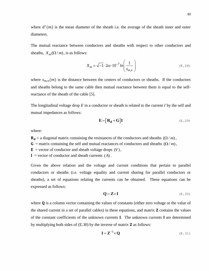
89
where is the mean diameter of the sheath i.e. the average of the sheath inner and outer
diameters.
The mutual reactance between conductors and sheaths with respect to other conductors and
sheaths, ( / )mX m , is as follows:
7
,
11 2 10m
m n
X lns
(E.28)
where is the distance between the centers of conductors or sheaths. If the conductors
and sheaths belong to the same cable then mutual reactance between them is equal to the self-
reactance of the sheath of the cable [5].
The longitudinal voltage drop in a conductor or sheath is related to the current by the self and
mutual impedances as follows:
dE R G I (E.29)
where:
= a diagonal matrix containing the resistances of the conductors and sheaths ( / )m ,
= matrix containing the self and mutual reactances of conductors and sheaths ( / )m ,
= vector of conductor and sheath voltage drops ( )V ,
= vector of conductor and sheath currents ( )A .
Given the above relation and the voltage and current conditions that pertain to parallel
conductors or sheaths (i.e. voltage equality and current sharing for parallel conductors or
sheaths), a set of equations relating the currents can be obtained. These equations can be
expressed as follows:
Q Z I (E.30)
where is a column vector containing the values of constants (either zero voltage or the value of
the shared current in a set of parallel cables) in these equations, and matrix contains the values
of the constant coefficients of the unknown currents . The unknown currents are determined
by multiplying both sides of (E.30) by the inverse of matrix as follows:
1 I Z Q (E.31)
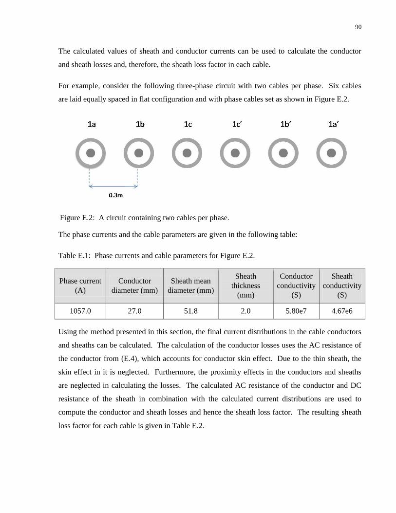
90
The calculated values of sheath and conductor currents can be used to calculate the conductor
and sheath losses and, therefore, the sheath loss factor in each cable.
For example, consider the following three-phase circuit with two cables per phase. Six cables
are laid equally spaced in flat configuration and with phase cables set as shown in Figure E.2.
Figure E.2: A circuit containing two cables per phase.
The phase currents and the cable parameters are given in the following table:
Table E.1: Phase currents and cable parameters for Figure E.2.
Phase current
(A)
Conductor
diameter (mm)
Sheath mean
diameter (mm)
Sheath
thickness
(mm)
Conductor
conductivity
(S)
Sheath
conductivity
(S)
1057.0 27.0 51.8 2.0 5.80e7 4.67e6
Using the method presented in this section, the final current distributions in the cable conductors
and sheaths can be calculated. The calculation of the conductor losses uses the AC resistance of
the conductor from (E.4), which accounts for conductor skin effect. Due to the thin sheath, the
skin effect in it is neglected. Furthermore, the proximity effects in the conductors and sheaths
are neglected in calculating the losses. The calculated AC resistance of the conductor and DC
resistance of the sheath in combination with the calculated current distributions are used to
compute the conductor and sheath losses and hence the sheath loss factor. The resulting sheath
loss factor for each cable is given in Table E.2.

91
To verify the accuracy of the method in the calculation of the sheath loss factors for the above
case, the same configuration was simulated in Ansoft Maxwell. The results are also given in
Table E.2, which shows excellent agreement between both approaches.
Table E.2: Sheath loss factors for cables in Figure E.1, computed using the approach in this
section and a numerical method program Ansoft Maxwell.
Cable # 1a 1b 1c 1c‟ 1b‟ 1a‟
Sheath loss
factor 1.57 0.77 1.46 1.46 0.77 1.57
Ansoft 1.56 0.77 1.45 1.45 0.77 1.56
The method summarized in this section is tested through a sensitivity analysis of the cable
separations. It was determined that the accuracy of the results generally decreased with
decreasing cable separation, probably because the method ignores the variation of the current
density within each sheath caused by the proximity effect. However, the method is reasonably
accurate for most practical distances of interest; the practical distance being no less than about
20cm based on simulations. This distance is practical for the separation of two cables, where
each cable is laid inside a duct. However, for smaller cable separation distances, a more accurate
way for calculating the losses would be to approximate the sheaths and conductors with multiple
physical thin wires and the method of filaments is used for these wires as discussed in Section
2.3.

92
Appendix F
The Barrier method algorithm for solving convex optimization problems
This appendix briefly presents the barrier-method algorithm for solving convex optimization
problems, such as that given by (3.2) for calculating the ampacities of multiple cables with fixed
locations.
The convex optimization problem in (3.2) is of the following form:
0
0 1, ,i
Minimize f (x)
subject to f (x) i n
where 1 2T
nx I I I , 0f (x) and if (x) are polynomial functions in x . The equality
constraints are implicitly enforced by assigning the same current variable name to cables
belonging to the same phase of the circuit.
Optimization problems consisting of a linear objective function and inequality quadratic
constraints can be solved effectively using the barrier method algorithm, as follows:
Given: strictly feasible x , (0) , 1t t , tolerance 0out
Repeat:
1. Compute the solution of 0
1 Minimize f (x)
t
, *( )x t , starting at x , using Newton‟s
method as follows:
Given: starting point feasible *x , ( *x x ), tolerance 0in , 1
0, , 0,12
.
Repeat:
a. Compute *x by solving the matrix equation:

93
*
2 * 2 * * * *0 0
( )
1 1( ) ( ) ( ) ( )
r x
f x x x f x xt t
b. Compute damping factor int for updating *x :
c. Update * * *inx x t x .
d. Stopping criterion: stop if *innorm r x .
2. Update *( )x x t
3. Stopping criterion: stop if / outn t
4. Increase .t t
where
1
log
n
i
i
( f (x))
. 0f and 20f are the gradient and hessian of the objective
function 0f respectively and and 2 are the gradient and hessian of the function
respectively.
* * *
1
1
in
in in
in in
t
while norm r x t x t norm r x
t t

94
Appendix G
VIS customization for best-ampacity-configuration optimization
This appendix describes the VIS algorithm customization for determining best ampacity cable
configuration (relevant to the discussion in Section 3.3).
The customization of the VIS algorithm steps depicted in Figure 3.4 is described in the following
points.
1) Encoding and random generation: Each different cable configuration is a viable solution to
the combinatorial optimization problem, and should be unique in its representation as a solution
candidate in the VIS algorithm. Because the cable configurations are simply the positions of the
cables in fixed ducts, a natural way of representing each configuration is through a sequence of
cable identifiers. Each identifier is assigned to a specific cable, and each position within the
sequence is preset to a specific duct. An illustration of the sequence corresponding to a cable
configuration is shown in Figure G.1.
The identifiers specify the cable circuit and phase. If there are multiple cables per phase, they
are distinguished through the addition of an extra apostrophe. For example, the identifier “ 1a‟ ”
represents one of the two cables belonging to phase “a” of circuit 1, the other cable having the
identifier “ 1a ”. If there is no cable filling a particular duct, then this non-existent cable is
represented by a zero, “ 0 ”. As can be seen in Figure G.1 each duct contains a cable identifier.
Each duct is also preset to a position in the sequence. This preset position is given by a number
at the top left corner of the duct, corresponding to a position index within the sequence going
from left to right.

95
Figure G.1: Duct bank installation showing twelve cables in fifteen ducts and the corresponding
sequence representation
In the first step of the algorithm, a number of allowable sequences, popN , are generated
randomly to represent the initial population. Next, the population undergoes cloning and
mutation operations in the inner loop of the algorithm, as discussed next.
2) Mutation: Evolutionary algorithms explore the solution space generally through crossover
and mutation of the population. However, algorithms that are based on the immune system do
not have a crossover analogy, and, thus, only mutation is implemented in the VIS solution.
Mutation is achieved basically through random local modifications of each sequence. The
mutation operation should be closed—i.e., the resulting sequence should also be legal. Two
mutation operations are implemented in the algorithm—namely, Exchange and Inversion. These
two operations are detailed below.
The Exchange mutation operation exchanges the contents of two random elements in the
sequence. This operation is illustrated in Figure G.2.

96
Figure G.2: Exchange mutation operation
As can be seen in Figure G.2, two elements are exchanged such that the cable in duct “11” is
removed and placed in the previously empty duct “14”.
Inversion mutation is implemented by choosing two random edges within the sequence and
reversing the order of the elements in between. This operation is illustrated in Figure G.3.
As can be seen from Figure G.3, the cables inside ducts “3”-“6” are reversed in order.
Figure G.3: Inversion mutation operation
3) Fitness: The measure of fitness in our problem is the total ampacity, which is computed using
the method discussed in Section 3.2.1 for each cable configuration. Depending on whether the
objective is to minimize or maximize the total ampacity, a solution with a better fitness will have
a lower or higher total ampacity, respectively.
4) Affinity, Suppression, and Random Replacement: The affinity and suppression operations
implemented in [19] are based on comparing sequences together, element by element, and
determining how many elements differ. If the two sequences differ by less than a preset
threshold number of elements, then one of the sequences is deleted and replaced by a randomly
generated one. These operations filter out any similar sequences in the population.

97
However, this approach does not result in optimal performance for the problem being solved
here. This is because two sequences differing by just two elements can correspond to two
different cable configurations with a large difference in the total ampacity. Thus, the suppression
operation is implemented by making an exact comparison between every two sequences. If the
two sequences are exactly the same, then one of them is deleted and replaced by a randomly
generated new one.

98
Appendix H
Comparison of the VIS algorithm approach with the brute-force method for a practical duct bank installation
This appendix provides an assessment of the accuracy of the VIS results in comparison with the
brute-force solutions, for a duct bank installation shown in Figure H.1.
Figure H.1: Duct bank installation for comparing VIS results with brute-force solutions
The cable configuration for the largest total ampacity is obtained using both the VIS approach
and using the brute-force method of solving all possible configurations. The brute-force process
results in 12 different configurations that have the same largest total ampacity (due to
symmetry). One of these configurations is shown in Figure H.2. The VIS program is invoked
with the same parameters as in Section 3.4.1 but with the inner and outer iterations both set to 8.
Ten independent reruns of the VIS program, from scratch with new starting random population,
result in the final solutions that belong to the subset of 12 optimal configurations obtained using
the brute-force method. The VIS method requires 6 minutes to simulate whereas the brute-force
method takes about 5 hours. These results show that although the VIS approach searches only a
portion of the total solution space (about 2% of the total space for this problem), the VIS
program final answer is the global optimum and is obtained in a significantly shorter time than
with the brute-force method.

99
Figure H.2: Global optimum configuration for the largest ampacity, obtained using both the VIS
and the brute-force approaches


![Ch5 Underground Power Cables 2[1]](https://static.fdocuments.net/doc/165x107/54e826974a7959704f8b4920/ch5-underground-power-cables-21.jpg)