CONDUCTANCE OF SUPERCONDUCTOR-NORMAL METAL CONTACT JUNCTIONBEYOND QUASICLASSICAL APPROXIMATION

BY

VLADIMIR LUKIC

BSc, University of Belgrade, 1997

DISSERTATION

Submitted in partial fulfillment of the requirementsfor the degree of Doctor of Philosophy in Physics

in the Graduate College of theUniversity of Illinois at Urbana-Champaign, 2005

Urbana, Illinois

c© Copyright by Vladimir Lukic, 2005

CONDUCTANCE OF SUPERCONDUCTOR-NORMAL METAL CONTACT JUNCTIONBEYOND QUASICLASSICAL APPROXIMATION

Vladimir LukicDepartment of Physics

University of Illinois at Urbana-Champaign, 2005Anthony J. Leggett, Advisor

The subject of this thesis is a study of the superconductor-normal metal (SN) contact

junction by systematically treating the corrections of the order ∆/EF in momentum and

conductance. We isolated the effects that are already present in the original formulation of

Blonder-Tinkham-Klapwijk (BTK) model, but were neglected as the small quantities of the

order ∆/EF .

The corrections studied are: non-equal momenta of various particles in the system, self-

consistent finite gap onset length scale, non-exact retro-reflection in Andreev process of the

particles with finite energy, non-trivial renormalization of the barrier potential due to the

non-equal momenta at finite incidence angle, and effects due to an anisotropy of the systems

in contact. The main question is what is the interplay of these effects, and can they con-

structively add to produce the effect of the order 1. The answer required treatment of all the

effects from the outset at the same level, and incorporation of these effects in a self-consistent

calculation. To achieve that, a new method for self consistent calculation of the behavior

of gap at the SN contact is developed, which does not use the quasiclassical approximation,

but rather finds solution to the Bogoliubov - De Gennes equations in a simplified, step-wise

constant, model of the gap. The conductance is calculated using the same method, thus

guaranteeing the same accuracy.

A study of self-consistently obtained solution shows that these corrections often have an

effect opposite to each other, or have the same target states, which limits the overall effect.

As a consequence even for large ∆/EF the overall correction is still relatively small, and the

conductance of the system does not differ much from the simple BTK model. We have thus

shown the reason for robustness of BTK model, and gained a better view of what might be

the cause of larger discrepancies between this simple model and experiment.

iii

To my family.

To Maki.

iv

Acknowledgments

Thanks to my advisor Tony Leggett, for his patience while I was trying to find myself in

physics (and world in general), and for the innumerable sound advices he gave me during

all these years. Thanks to Jim Eckstein and Laura Greene, who taught me how to perceive

physics from the experimental side. Thanks to my friends and collegues - Joseph Jun,

Geoffrey Warner, Vivek Aji, Carl Tracy, Argyrios Tsolakidis, Julian Velev. Thanks to to my

family - Veljko, Milica and Natasa, for everything. Thanks to Pero, Momir, Zarija, Tijana,

Dimitrios, Nemanja, Sale...to all my friends. Most of all, thanks to Maki.

I acknowledge financial support from the National Science Foundation under grants NSF

DMR 03-50842, NSF DMR 99-86199, NSF DMR 96-14133, NSF DMR 91-2000COOP, from

MRL DOE grant, and from the Department of Physics, University of Illinois.

v

Table of Contents

List of Figures . . . . . . . . . . . . . . . . . . . . . . . . . . . . . . . . . . . . . . . viii

Chapters

1 Introduction . . . . . . . . . . . . . . . . . . . . . . . . . . . . . . . . . . . . . . . 1

1.1 Superconductor-Normal Metal Contact Junctions and Andreev Reflection . . 2

2 The Bogoliubov-De Gennes Equations and the Blonder-Tinkham-Klapwijk Model 8

2.1 Bogoliubov - DeGennes Equations . . . . . . . . . . . . . . . . . . . . . . . . 8

2.2 The Model of Blonder, Tinkham and Klapwijk . . . . . . . . . . . . . . . . . 10

3 The Nature of Gap Edge Conductance Peak, Subgap Conductance and Zero-Bias

Properties . . . . . . . . . . . . . . . . . . . . . . . . . . . . . . . . . . . . . . . . 21

4 Corrections to the BTK Conductance . . . . . . . . . . . . . . . . . . . . . . . . . 28

4.1 Finite Gap Onset Length and Exact Momenta . . . . . . . . . . . . . . . . . 30

4.2 Non-exact Retro-reflection . . . . . . . . . . . . . . . . . . . . . . . . . . . . 32

4.3 Angle Dependence of Effective Barrier Strength . . . . . . . . . . . . . . . . 36

4.4 Corrections Not Taken into Account . . . . . . . . . . . . . . . . . . . . . . 44

5 Calculation of the Conductance . . . . . . . . . . . . . . . . . . . . . . . . . . . . 47

5.1 Particle with Perpendicular Incidence Angle . . . . . . . . . . . . . . . . . . 47

5.2 Finite Incidence Angle . . . . . . . . . . . . . . . . . . . . . . . . . . . . . . 56

6 Self-consistent Gap Calculation . . . . . . . . . . . . . . . . . . . . . . . . . . . . 60

6.1 Quasi-classical Self-consistent Gap Calculations . . . . . . . . . . . . . . . . 61

6.2 Improvement on Quasiclassical Approach . . . . . . . . . . . . . . . . . . . . 64

vi

7 Results and Interpretation . . . . . . . . . . . . . . . . . . . . . . . . . . . . . . . 73

7.1 Effects of Finite Gap Onset Length . . . . . . . . . . . . . . . . . . . . . . . 76

7.2 Effects of Mismatch and Anisotropy on Fermi Surface . . . . . . . . . . . . . 82

7.3 Effects of Non-exact Retro-reflection . . . . . . . . . . . . . . . . . . . . . . 83

7.4 Effects of Self-consistence . . . . . . . . . . . . . . . . . . . . . . . . . . . . . 84

8 Conclusions . . . . . . . . . . . . . . . . . . . . . . . . . . . . . . . . . . . . . . . 86

Appendix

A Quantum Mechanical Ramp Barrier . . . . . . . . . . . . . . . . . . . . . . . . . . 88

A.1 Exact Solution of the Tunneling Problem . . . . . . . . . . . . . . . . . . . . 88

A.2 Numerical Results and Comparison of the Solutions . . . . . . . . . . . . . . 90

B Basic Quasiclassical Equations . . . . . . . . . . . . . . . . . . . . . . . . . . . . . 94

C Definition and Calculation of Gap . . . . . . . . . . . . . . . . . . . . . . . . . . . 96

References . . . . . . . . . . . . . . . . . . . . . . . . . . . . . . . . . . . . . . . . . . 98

Author’s Biography . . . . . . . . . . . . . . . . . . . . . . . . . . . . . . . . . . . . . 100

vii

List of Figures

1.1 SN (A) and SIN (B) junction. Dashed regions are occupied states.Grey block

is an interface barrier. Single particle states are not allowed inside the gap. . 3

1.2 Four processes occurring at SN interface: specular reflection (A), Andreev

reflection (B), transmission as an electron (C), transmission as a hole (D).

Arrows point in a direction of the velocity of the particle, and abbreviations

for the directions are: eR - a right moving electron, eL - a left moving electron,

hR - a right moving hole, hL - a left moving hole. Electron trajectories - full

line, hole trajectories - dashed line. . . . . . . . . . . . . . . . . . . . . . . . 6

2.1 Energy spectrum of BdG equations. Four types of particles with the given

energy E are marked by the dots: left moving electron-like (eL), right moving

hole-like (eL), left moving hole-like (hL), right moving electron-like (eR). . . 10

2.2 Visualisation of the BTK problem. The properties of N and SC are uniform,

and there is a δ-function potential at the boundary. . . . . . . . . . . . . . 12

2.3 The BTK conductance normalized to a high voltage value, for values of Z

(top to bottom curve): 0, 0.3, 0.6, 1.0, 2.0. . . . . . . . . . . . . . . . . . . 15

2.4 The BTK conductance normalized to a normal state conductance of a system

without barrier for values of Z (top to bottom curve): 0, 0.3, 0.6, 1.0, 2.0. . 15

2.5 The conductance contributions from the individual components, Z = 0, EF =

1eV , ∆ = 20meV : (upper row) a - transmission without branch crossing, b

- transmission with branch crossing, (lower row) c - Andreev reflection, d -

specular reflection. The coefficient b and c are zoomed up to a larger scale to

stress that they are exactly zero in BTK. . . . . . . . . . . . . . . . . . . . . 17

viii

2.6 Contribution to the conductance from the individual components, Z = 2,

EF = 1eV , ∆ = 10meV : (upper row) a - transmission without branch cross-

ing, b - transmission with branch crossing, (lower row) c - Andreev reflection,

d - specular reflection. . . . . . . . . . . . . . . . . . . . . . . . . . . . . . . 18

2.7 Temperature dependence of s-wave BCS gap, and the smearing factor ∂f/∂V . 19

2.8 Temperature dependence of the BTK conductance given for Z=0 (left) and

Z=0.5 (right). Curves from the bottom correspond to T=0, 0.2Tc, 0.4Tc,

0.6Tc, 0.8 Tc, Tc. Each curve is offset by +1 from the previous one. We use

µ = 1eV , ∆ = 10meV . . . . . . . . . . . . . . . . . . . . . . . . . . . . . . . 20

2.9 The plots of a zero bias conductance as a function of temperature, normalized

to a high voltage value, for different values of Z - from top: Z=0, 0.3, 0.6, 0.9,

1.2, 1.5. . . . . . . . . . . . . . . . . . . . . . . . . . . . . . . . . . . . . . . 20

3.1 SN junction with a displaced barrier. Three processes represent possible tra-

jectories after AR at the SC interface. The barrier position is a vertical line

with T,R, interface is at the gap onset. . . . . . . . . . . . . . . . . . . . . . 24

4.1 Point contact conductance between Au and c-axis of CeCoIn5, from [14]. . . 29

4.2 A comparison of the BTK conductance (full line) to the similar calculation

with gap onset length ξ, and µ = 1eV , ∆ = 10meV , Z = 0 (left) and

Z = 0.367 (right). Note that y-axis doesn’t start at zero. . . . . . . . . . . . 31

4.3 Andreev reflection for a particle above Fermi surface. . . . . . . . . . . . . . 33

4.4 Particles on the outside of the space limited with lines AB and CD cannot

AR (momenta k1 and k2). Particle k3 is allowed to AR. Left hand side is a

case kFSC > kFN , right side kFSC < kFN . . . . . . . . . . . . . . . . . . . . . 34

4.5 The effect of limited tunneling due to the non-exact retro-reflection in a system

with µ = 1eV , ∆ = 10meV , T = Tc/2 = 33K in a dirty limit (lower curve)

compared to the finite temperature BTK calculation (upper curve). . . . . . 35

4.6 Limit on retro-reflection as given by (4.4) - kmax =√

2kF . . . . . . . . . . . 36

4.7 A contact of two metals with different Fermi wavevectors. Tunneling to (and

from) regions above the line AB and below CD is forbidden. Note that k‖ is

conserved. . . . . . . . . . . . . . . . . . . . . . . . . . . . . . . . . . . . . . 38

ix

4.8 Angle dependence of Zeff for Z0 = 0, m1/m2 = 5 and values of EF1/EF2, from

the bottom curve: 2, 1, 1/2, 1/5, 1/8, 1/10. . . . . . . . . . . . . . . . . . . 39

4.9 Zeff as a function of incident angle, for a system with m1/m2 = (1 + 4 cos θ)

and ratio EF1/EF2 (from the left): 20, 10, 5, 3, 2.5, 2. . . . . . . . . . . . . . . 41

4.10 Zeff as a function of incident angle, for a system with m1/m2 = (1 + 4 cos θ)

and ratio EF1/EF2 (from the left): 2, 1, 1/2, 1/5, 1/10, 1/20. . . . . . . . . . . 42

4.11 Effect of the proper inclusion of the angle dependent Z, for a system with Z0

= 0.1, rk = 2/3. Dots: calculation with correction taken into account; full

line - BTK calculated with corresponding Zeff = 0.367. . . . . . . . . . . . . 43

5.1 Schematics of approximation of a real potential by a piecewise constant model

potential. . . . . . . . . . . . . . . . . . . . . . . . . . . . . . . . . . . . . . 48

5.2 One segment with corresponding particle amplitudes. . . . . . . . . . . . . . 50

5.3 Components of the conductance for a system with step-function gap and exact

momenta retained throughout the calculation, with Z = 0, µ = 1eV , ∆ =

0.2eV (upper row): a-transmission without branch crossing, b - transmission

with branch crossing, (lower row) c - Andreev reflection, d- specular reflection.

Note a different scale in parts c and d. Compare with Fig.2.5 to see an effect of

exact momenta. Vertical axes - current, normalized to the incoming particle;

horizontal axes - energy, in units 0.1meV . . . . . . . . . . . . . . . . . . . . 54

5.4 Distribution of the current in space for each component eR, eL (upper row),

hR, hL (lower row), normalized to the incoming eR current. Z = 0.7, µ = 1eV ,

∆ = 0.1eV . An electron is incoming from the right, position of the barrier is

at the mark 50. Length ξ is 10 divisions on x axis. . . . . . . . . . . . . . . . 55

5.5 Schematics of the change of incident angle for a sequence of segments, due to

the increase of gap at the barrier, as calculated in (4.12) . . . . . . . . . . . 58

6.1 Boundary conditions for a SN contact: an electron incoming from the left (A)

and a hole outgoing to the right (B). Full line - electron, dotted line - hole.

Arrows point in the direction of propagation. N metal is on the left side of

the interface in both figures. . . . . . . . . . . . . . . . . . . . . . . . . . . . 65

x

6.2 Processes (A) and (B) from the Fig.6.1 drawn to include AR along the tra-

jectory (left). Contributions to the gap from two trajectories at every point

in space (right). . . . . . . . . . . . . . . . . . . . . . . . . . . . . . . . . . 68

6.3 The unnormalized contribution to the pair correlation function (6.5) from the

particles of one energy and along one incident angle for Nb, Z=0, T=0 (E ≈ ∆

(left), E ≈ 3∆ (right)). Units on x-axis are 1/10ξ, and contact is at the mark

100, N is to the left, SC to the right of it. . . . . . . . . . . . . . . . . . . . . 69

6.4 The unnormalized contribution to the pair correlation function from particles

at an incident angle θ = 0 (left) and integrated over all angles (i.e. after

complete first iteration) for Nb, Z=0 (E ≈ ∆ (left), E ≈ 3∆ (right). Units

on x-axis are 1/10ξ, and contact is at the mark 100. . . . . . . . . . . . . . . 70

6.5 The calculated gap in each iteration (top to bottom) (right) and the unnor-

malized pair correlation function after three iteration loops (left) for Nb, Z=0

. Units on x-axis are 1/10ξ, and contact is at the mark 100. . . . . . . . . . 70

6.6 Self-consistent gap and normalized pair correlation function for T = 0.95Tc,

all parameters are the same as in other figures. . . . . . . . . . . . . . . . . . 71

6.7 Self-consistent gap and normalized pair correlation function for barrier para-

meter Z = 4.0, T = 0, all parameters the same as in other figures. . . . . . . 71

6.8 Self consistent gap after 4 iterations for EF = 1eV and ∆ = 0.1eV (left) and

∆ = 0.2eV (right) at T=0, Z=0. . . . . . . . . . . . . . . . . . . . . . . . . . 72

7.1 Evolution of the conductance curve formSC/mN = (1+4 cos θ) and EFSC/EFN

1/5, 1/2 (upper row), 2, 3 (lower row). EF = 1eV , ∆ = 10meV , Z0 = 0. Full

line is BTK curve, fitted to the high energy values, dotted line is this cal-

culation. Vertical axis is a conductance, normalized to a perfect contact,

horizontal - energy, in units 1/100∆. . . . . . . . . . . . . . . . . . . . . . . 74

7.2 A conductance curve for mSC/mN = (1+4 cos θ) and EFSC/EFN - 2 (left)and

3 (right) . Z0 = 0, EF = 1eV , ∆ = 100meV (upper row) and ∆ = 200meV

(lower row). Full line is BTK curve, fitted to the high energy values, dotted

line is this calculation. Vertical axis is a conductance, normalized to the

perfect contact, horizontal - energy, in units 1/100∆. . . . . . . . . . . . . . 75

xi

7.3 A comparison of the self-consistent calculation of the gap for a system with

mSC/mN = (1 + 4 cos θ) and EFSC/EFN - 0.2 (dots) and 3 (full line), after

four iterations. Vertical axis is gap in eV , horizontal is distance in units 1/10ξ

- contact at 50. . . . . . . . . . . . . . . . . . . . . . . . . . . . . . . . . . . 75

7.4 Evolution of the subgap structure with incident angle, Z=1.3, Ef = 1eV , ∆ =

1meV : full line - BTK, dots - this calculation, normalized so that conductance

at high voltage without barrier is σ0 = 1. Consequence of this normalization

is that subgap conductance σSN(E) = 2 means that particle at that energy

does not feel the presence of the barrier. . . . . . . . . . . . . . . . . . . . . 77

7.5 The schematics of the model of slowly varying gap. N - normal side, SC -

superconducting side (with gap ∆). Region R is either superconducting (with

gap ∆ < ∆SC), or normal (∆ = 0). . . . . . . . . . . . . . . . . . . . . . . . 78

7.6 The schematics of the condition (7.6): (A) - side view (distance vs. energy),

(B) - view from the above. A thick vertical line is a surface barrier, a thin

line is the position where Andreev reflection occurs . . . . . . . . . . . . . . 81

7.7 Conductance at very large incident angle θ > 88o, Z = 1.3, Ef = 1eV ,

∆ = 1meV . Full lines are BTK formula. Dots are calculation without (left)

and with (right) k = kf approximation. The normalization is the same as

above. . . . . . . . . . . . . . . . . . . . . . . . . . . . . . . . . . . . . . . . 82

A.1 Ramp potential in standard quantum-mechanical problem. We set V0 = 0.01eV . 89

A.2 The reflection coefficient of a ramp potential for U = 0.01eV , and values of

L = 0, 10, 20, 40, 80, 160, 320, 640A (descending curves). . . . . . . . . . . . . 90

A.3 A numerical approximation to the real potential form Fig. A.1 (steps), and

the ramp potential (straight line), for n = 10 steps. . . . . . . . . . . . . . . 91

A.4 Fitting the conductance on the energy scale of a gap. Full line - the exact solu-

tion of the ramp potential problem, dots - the numerical solution. U=0.01eV,

L=10A (upper curve) and L=320A (lower curve) . . . . . . . . . . . . . . . 92

A.5 Fitting the conductance on a very small scale - energy axis is offset so that

gap energy is at zero. Note that R-axis shows details smaller than Fig. A.4.

Full line - the exact solution, dots - the numerical solution. U=0.01eV, L=320A 93

xii

Chapter 1

Introduction

Transport phenomena in a point contact junction between superconductor and normal metal

are dominated by Andreev reflection, a process that transforms an electron into a hole that

retraces the path of an incoming particle. Theoretical description of the conductance of this

system is given by Blonder, Tinkham and Klapwijk, in a theory that is usually referred to as

BTK. Their approach is very simple, requires a single fitting parameter, yet it is extremely

successful. There are many corrections to this equation, but they usually do not produce

significant departures from BTK, and are therefore neglected.

In cases when BTK description is not satisfactory, one may try adding additonal fitting

parameters, such as quasiparticle lifetime. Addition of an extra fitting parameter adds new

fitting curves to the BTK family, but it is not always physically justified. One would natu-

rally like to avoid addition of a new free variable to the data fit.

There is a class of corrections to BTK that does not introduce a new physical effect to the

problem. One can study the physics already there with a higher accuracy. These corrections

do not introduce a new fitting parameter, but they do change family of functions described

by it. In essence, they provide a better fitting functions than BTK for same problem. The

purpose of this work is study of such one-parameter corrections.

The basic problem is that we know of several corrections to BTK of the order ∆/EF ,

and none of them has significant effect...but how do they act together? Do they add inde-

pendently, do they mutually enhance, or suppress? In particular, for a system with ∆/EF

1

of the order several percent, can these corrections add to produce a result of the order 1? To

answer, we will have to treat all corrections on the same level from the beginning and account

for them self-consistently. The answer turns out not to be spectacular - the corrections tend

to cancel each other out, but we can answer how does it happen, and the reasons for it are

interesting. To some extent, we managed to explain why is the BTK so robust and effective.

The motivation for this topic was real life problems of the experimental groups in Urbana.

Point contact junctions conductance data often look surprisingly similar to BTK, but they

are not exactly the same - and the discrepancy cannot be accounted for easily. Depending

on the geometry of the device, ordinary BTK can be twisted into an unrecognizable form. I

cannot say that I managed to describe said experiments well, but it was a great inspiration

for the work, and a pointer to what type of result is interesting to find.

The outline of the thesis is as follows: in the rest of Chapter 1 we will discuss phenom-

enological aspects of Andreev reflection without a quantitative approach. Chapter 2 is a

review of BTK, which we will use as a standard for comparison of all results. Chapter 3 is

a study of the origin of various aspects of BTK. Chapter 4 is a discussion of the corrections

introduced, and isolated effects of each correction separately. Chapter 5 is a discussion of

the algorithm used to calculate the conductance with a given gap profile. Chapter 6 is a

self-consistent calculation of the gap profile using a similar algorithm. Chapter 7 gives results

for the combination of effects and a discussion of their influence on each other, and Chapter

8 is a brief conclusion.

1.1 Superconductor-Normal Metal Contact Junctions and Andreev

Reflection

Contact between superconductor and normal metal can be in two different regimes - a tunnel-

ing junction (also called SIN junction) and a contact junction (SN junction). The difference

between them stems from the properties of the interface. A clean interface (one with no

potential barrier or impurities), which is considerably harder to make, results in a contact

2

Figure 1.1: SN (A) and SIN (B) junction. Dashed regions are occupiedstates.Grey block is an interface barrier. Single particle states are not allowedinside the gap.

regime - particles ballistically propagate between two metals. Interface with a potential

barrier - an insulating layer (therefore SIN)- produces junction in a tunneling regime. An

insulating barrier is usually consequence of a naturally occuring oxide at a metal surface, but

it can also be artificially produced. In a tunneling junction (Fig.1.1 (B)), normal metal (N)

and superconductor (SC) are largely independent of each other, their wave function overlap

is exponentially small and can be treated as a perturbation in a standard method called the

tunneling Hamiltonian approach [1]. In this regime the internal states of SC and N are to a

large extent unaffected by a system on the other side of a junction (though there are situa-

tions where it can be very important, e.g. [2]), and we usually observe how does the given

state influence a particle tunneling from the other side. We find, e.g., that a particle with

energy E smaller then a SC gap ∆ cannot penetrate the SC side, since there are no available

final states for it. Until we give a particle sitting at the Fermi surface enough energy (as an

electric potential offset V ) to reach the gap, there is no charge transfer between two systems

(in case of s-wave SC), and conductance σ = dI/dV = 0. Only for V > ∆ does transport

occur, and we find that conductance measurements effectively map the density of states of

a SC system.

3

In a contact junction (Fig.1.1 (A)), on the other hand, two systems are in a direct physical

contact, and overlap of the wave functions is large. One cannot apply perturbation theory,

but rather has to match the wave functions and solve the problem of two systems in contact

simultaneously. Influence of two systems on each other is much larger than in the SIN case,

and the state of a system near the contact is significantly different from that of an isolated

sample. The mutual effect of SC and N system in SN junction is called the proximity effect.

To study the transport of SN contact properly, one takes into account not only the influence

of a, say, SC state on a particle incoming from a N side, but also the other way around -

effect of the particles from N on the ground state of SC system. It is this problem that we

shall study in the present work.

The dominant effect in a subgap transport (energies E < ∆) in an SN contact junction

and the main cause of proximity effect is Andreev reflection. Andreev reflection (AR) is a

process in which the incoming electron gets reflected as a hole, nearly retracing the trajectory

of the electron. This type of reflection is also called retroreflection. Opposite conversion,

hole into electron, is also possible, but to be definite we shall discuss electron to hole AR

only. Minor differences between two processes will be addressed later.

AR is a process typical of superconducting state, and most prominent in area around an

SN contact. Its overall effect is the transfer of a pair of electrons from N to SC side. Since

only pairs exist in SC at energies E < ∆ and T = 0, this is the only transfer mechanism in

that energy range. An incoming electron with momentum k and E < ∆ can be transfered

to SC, only if it finds a single electron of the opposite momentum −k and forms a Cooper

pair. Since free electrons are not available in SC at that energy, the pairing electron must

come from the N side, leaving behind a hole with the momentum −k.

This effect was first studied by Andreev [3] in order to explain the anomalous heat con-

duction properties at SN contact. Saint-James [4, 5] was the first to study its influence on

transport of charge in SN junction, independently of Andreev’s work. Sometimes the An-

dreev effect used in this context is called Andreev-Saint-James effect [6].

4

If there is a finite barrier at SN interface, a particle can also get specularly reflected

with E < ∆. The particles with energy E > ∆ can be transmitted as electron- or hole-like

quasiparticles into SC. While details of these processes will be given later in Sec.2.2, we can

now note how these processes change perpendicular (v⊥) and parallel (v‖) components of

the velocity (relative to the interface) for two systems in contact with the identical Fermi

surfaces, the same Fermi energy EF and the same effective mass m. These four processes

exhaust all possibilities. In Fig.1.2 we see that these changes are:

• specular reflection : v⊥ → −v⊥, v‖ → v‖

• Andreev reflection : v⊥ → −v⊥, v‖ → −v‖

• transmission as an electron : v⊥ → v⊥, v‖ → v‖

• transmission as a hole : v⊥ → v⊥, v‖ → −v‖

Process of transmission as a hole might look counterintuitive, but one should bear in mind

that the parallel component of the momentum has to be conserved, and it is conserved in

all four processes listed here - by virtue of the fact that the momentum of a hole is opposite

to its direction of propagation.

While the presence of a gap is crucial for the AR, it should be noted that it works only for

a SC gap. A particle entering the region with semiconducting gap will be only specularly

reflected. The reason for this is in the very nature of a SC state. An electron entering a

semiconductor will have its wave function matched to that of a corresponding state in the

gap - which is just an exponentially decaying electron wave function. The hole wavefunction

does not play a role, since neither N nor semiconducting state mix electrons and holes. The

eigenstates of the SC are the coherent mixtures of electron and hole parts. Thus, an electron

entering a SC will have its wave function matched to a decaying part that has both electron

and hole in it. But, then, the hole part on the SC side has to be matched too, and the only

way to do it is to produce a hole wave function on the N metal side. That is the essence of AR.

The transfer of a pair into the SC by AR has the spectacular consequences for the

low-energy electrical transport properties of an SN contact. If an electron along the given

5

Figure 1.2: Four processes occurring at SN interface: specular reflection (A),Andreev reflection (B), transmission as an electron (C), transmission as a hole(D). Arrows point in a direction of the velocity of the particle, and abbrevia-tions for the directions are: eR - a right moving electron, eL - a left movingelectron, hR - a right moving hole, hL - a left moving hole. Electron trajecto-ries - full line, hole trajectories - dashed line.

6

trajectory is transmitted with the energy E > ∆, it carries a charge e to the other side.

Along the same trajectory an electron with E < ∆ is AR - thus transferring a charge 2e to

a SC. The conductance below the gap is increased by a factor 2! This is in great contrast

to a tunneling junction, where there is no charge transfer at all below the gap. There are

no single particle states available at E < ∆, but the pair states are available. Since AR

is a two-particle tunneling process, it is greatly suppressed in a SIN junction, since it is a

higher-order process compared to single particle tunneling. Note that this is in contrast to

an SIS junction - a pair tunneling in that case is a process of a same order as single par-

ticle tunneling (which is the basis of the Josephson effect). An SIS junction has correlated

systems on both sides of the barrier, and tunneling of one electron in a pair automati-

cally ensures tunneling of the other. It is not so in the SIN case - electrons on the N side

are uncorrelated, and they have to tunnel separately, making it a higher order process. The

barrier plays little role in an SN contact, since by definition it is orders of magnitude smaller.

It is this factor of 2 that plays a central role in the study of SN junctions. The method we

employ is simply shooting the electrons toward the barrier one by one at various angles and

energies, and calculating the probabilities for each of the processes listed above. While below

the gap the matter is simplified by the fact that no transmission is allowed (to the extent

that we can get BTK results without actually performing a microscopic calculation), above

the gap we have to take into account properly the combination of all possible processes. The

resulting solutions for the conductance are drastically different in the two energy ranges.

an If for a certain system every trajectory that is transmitted in an NN junction gets Andreev

reflected in SN contact - the overall conductance will have an increase by a factor 2 after the

SC transition. Our main task will be tracing the trajectories that are not Andreev reflected,

and in particular studying the factors not included in the original BTK that can change the

conditions for Andreev reflection. For that we will need a microscopic theory, which we shall

study in the following section.

7

Chapter 2

The Bogoliubov-De Gennes Equations and the

Blonder-Tinkham-Klapwijk Model

This section reviews briefly the Bogoliubov - DeGennes (BdG) equations, used to describe

a superconducting system near the boundaries and the inhomogeneities, and the theory by

Blonder, Tinkham and Klapwijk (BTK) that uses these equations to describe conductance

of a superconducting-normal metal (SN) contact. We will need only the simplest solution of

the BdG, that for an isotropic system.

2.1 Bogoliubov - DeGennes Equations

The Bogoliubov-De Gennes equations [7] are the mean-field equations for a superconducting

system. They are obtained as the equations of motion for the mean-field approximation

to BCS Hamiltonian. In their final form, they are coupled system of the two second-order

differential equations and the two self-consistence conditions:

Enfn(r, t) =

(− h2

2m

∂2

∂r2− µ(r) + U(r)

)fn(r, t) + ∆(r)gn(r, t)

Engn(r, t) = −(− h2

2m

∂2

∂r2− µ(r) + U(r)

)gn(r, t) + ∆(r)fn(r, t)

∆(r) = V Σnfn(r, t)g∗n(r, t) ∗ (1− 2n(En)) (2.1)

U(r) = ΣnU(r)|fn(r, t)|2 ∗ n(En) + |gn(r, t)|2 ∗ (1− n(En)))

8

where n = (1 + exp(−β(E − µ)) is the Fermi occupation factor, β = 1/kBT na inverse

temperature, µ a chemical potential (which, in principle, can be position dependent), U(r)

a single particle potential calculated in the normal metal, ∆ - BCS gap, and u and v - the

wave functions for an electron and a hole.

As written this system is impossible to solve in the general form. For a homogeneous,

clean system it yields the usual BCS value of the gap and the wavefunctions:

E2 = ∆2 + ε2q

fq = eiEt−qr ∗ u0

gq = eiEt−qr ∗ v0 (2.2)

u20 =

1

2

(1 +

√E2 −∆2

E

)v2

0 =1

2

(1−

√E2 −∆2

E

)BdG equations have the solutions for both positive and negative E, connected by (f, g)T (E) =

(−g∗, f∗)(−E). Since these are not independent, we will always deal with the positive en-

ergy solutions only, and therefore all the sums run over the positive values of energy unless

explicitly stated otherwise. For a given energy E we have four solutions propagating along

the direction r. The momentum q corresponding to these solutions is given by:

q± =

√2mSC

h2

√µ±

√E2 −∆2 (2.3)

The particles and their momenta are given in Fig.2.1. The names electron-like and hole-like

are referring to the corresponding solutions in ∆ → 0 limit, whereas in the SC state they

are really mixture of an electron and a hole component - a property explicitly captured in

the spinor representation (an electron component in the first row, a hole in second):

ψeR =

u0

v0

eiq+r;ψeL =

u0

v0

e−iq+r (2.4)

ψhR =

v0

u0

e−iq−r;ψhL =

v0

u0

eiq−r

Later, we will be interested in solving (2.1) in a more complicated case.

9

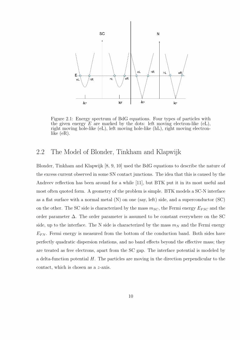
Figure 2.1: Energy spectrum of BdG equations. Four types of particles withthe given energy E are marked by the dots: left moving electron-like (eL),right moving hole-like (eL), left moving hole-like (hL), right moving electron-like (eR).

2.2 The Model of Blonder, Tinkham and Klapwijk

Blonder, Tinkham and Klapwijk [8, 9, 10] used the BdG equations to describe the nature of

the excess current observed in some SN contact junctions. The idea that this is caused by the

Andreev reflection has been around for a while [11], but BTK put it in its most useful and

most often quoted form. A geometry of the problem is simple. BTK models a SC-N interface

as a flat surface with a normal metal (N) on one (say, left) side, and a superconductor (SC)

on the other. The SC side is characterized by the mass mSC , the Fermi energy EFSC and the

order parameter ∆. The order parameter is assumed to be constant everywhere on the SC

side, up to the interface. The N side is characterized by the mass mN and the Fermi energy

EFN . Fermi energy is measured from the bottom of the conduction band. Both sides have

perfectly quadratic dispersion relations, and no band effects beyond the effective mass; they

are treated as free electrons, apart from the SC gap. The interface potential is modeled by

a delta-function potential H. The particles are moving in the direction perpendicular to the

contact, which is chosen as a z-axis.

10

They then consider an incoming particle from the N side. Upon incidence on the in-

terface, it undergoes the reflection (either as a particle or a hole) or the transmission (also

as a particle or a hole). The transmission is such that it does conserve the current, thus a

right-going particle on the N side will produce only a right going particles on the SC side.

We solve the BdG equations (2.1) separately on the SC and the N side, with the appropri-

ate parameters on each side and match the boundary conditions. Bogoliubov quasiparticles

on the SC side have weight u0 in the particle channel and v0 in the hole channel, while

particles on the N side have only one component (either particle or hole). The definition of

the particle momenta in the problem is:

k+ =

√2mN

h2

√EFN + E

k− =

√2mN

h2

√EFN − E

q+ =

√2mSC

h2

√EFSC +

√E2 −∆2 (2.5)

q− =

√2mSC

h2

√EFSC −

√E2 −∆2

where k+ is momentum of an electron on the N side, k− momentum of a hole on the

N side, q+ momentum of an electron-like quasiparticle on the SC side, and q− momentum

of a hole-like quasiparticle on the SC side. We solve the BdG equations separately in two

regions, and match the boundary conditions (see Fig.2.2): 1

0

eik+z0 + C

1

0

e−ik+z0 +D

0

1

eik−z0 = A

u0

v0

eiq+z0 +B

v0

u0

e−iq−z0

(2.6)

where on the left hand side (LHS) we have an incoming particle with the amplitude 1 (and

thus the probability equal to 1), and a reflected electron and a hole with the probabilities

C and D, both moving toward the left. On the right hand side (RHS) we have an outgoing

electron- and a hole-like quasiparticles with the amplitudes A and B, both moving to the

11

Figure 2.2: Visualisation of the BTK problem. The properties of N and SCare uniform, and there is a δ-function potential at the boundary.

right. For the derivatives, we have:

h2

2mN

ik+

1

0

eik+z0 − ik+C

1

0

e−ik+z0 + ik−D

0

1

eik−z0

= (2.7)

h2

2mSC

iq+A

u0

v0

eiq+z0 − iq−B

v0

u0

e−iq−z0

+

H ∗

A

u0

v0

eiq+z0 + B

v0

u0

e−iq−z0

where z0 is the position of the barrier, in the original problem z0 = 0, but this more general

form will be useful for the comparison with the later results.

The system (2.6), (2.7) is a system of four equations with four unknown variables - A,

B, C, D. Their physical meaning is that they are the amplitudes for:

• - a right going electron-like quasiparticle on the SC side: the amplitude for the trans-

mission without branch crossing (A)

• - a right going hole-like quasiparticle on the SC side: the amplitude for the transmission

with branch crossing (B).

12

• - a left going electron on the N side: the amplitude for the specular reflection (C)

• - a left going hole on the N side: the amplitude for the Andreev reflection (AR) (D)

’Branch crossing’ is the name we use for a tunneling process where the particle crosses

from an electron-like to a hole-like branch of the energy spectrum. In that sense the An-

dreev reflection is also a branch crossing process, but we shall exclusively use that name for

a transmitted particle.

The major simplification that BTK use to solve the system (2.6, 2.7) is setting k+ =

k− = kFN and q+ = q− = qFSC (though we will write these terms explicitely in the formulas

(2.10 - 2.14), in order to facilitate comparison with the corrections of the following chapters).

This induces the error of the order δk/kF =√E2 −∆2/2EF , thus of the order ∆/EF . Using

vSCF = hkFSC/mSC and vFN = hkFN/mN , we define Z0 = H/h

√vFN ∗ vFSC , and

Z2 ≡ Z2 = Z20 + (1− rv)

2/4rv

rv = vFN/vFSC =

√EFNmSC

EFSCmN

(2.8)

By using Z instead of Z0, we can set EFN = EFSC and mN = mSC . If the contact is

perfect (H = Z0 = 0) the effect of difference of the masses mSC and mN and the Fermi

energies EFSC and EFN is absorbed into the renormalized barrier strength Zeff through a

single parameter rv. Note that Zeff is insensitive to the exchange mSC ↔ mN , so it retains

the properties of a real barrier. To get the actual transmission coefficients for every branch

we have to take into account the difference in momenta and weight of a hole and a particle

part of the wavefunction. Thus we get:

a =(|A|2 ∗

(u2

0 − v20

)) q+SC

k+N

b = |B|2 ∗(u2

0 − v20

) q−SC

k+N

(2.9)

c = |C|2 d = |D|2 ∗ k−N

k+N

The solution of the system (2.6, 2.7) is very different in two regions E < ∆ and E > ∆,

13

as expected:

a(E) =

0 ; E < ∆

(u20−v2

0)u20(1+Z2)

γ2 ; E ≥ ∆b(E) =

0 ; E < ∆

(u20−v2

0)v20Z2

γ2 ; E ≥ ∆(2.10)

c(E) =

1− d = 4Z2(1+Z2)(∆2−E2)E2+(∆2−E2)(1+2Z2)2

; E < ∆

(u20−v2

0)Z2(1+Z2)

γ2 ; E ≥ ∆d(E) =

∆2

E2+(∆2−E2)(1+2Z2)2; E < ∆

u20v2

0

γ2 ; E ≥ ∆

where we defined γ = u20 + (u2

0 − v20)Z

2.

Knowing A, B, C and D, we can calculate the differential conductance of SC-N junction as:

σSC−N(E) = 2∗|D|2∗ k−N

k+N

+(|A|2∗(u20−v2

0))q+SC

k+N

+|B|2∗(u20−v2

0))q−SC

k+N

= 2∗d(E)+a(E)+b(E)

(2.11)

Since the total current through the junction has to be conserved (and equal to the current

carried by the incoming particle), the following condition is satisfied:

|C|2 + |D|2 ∗ k−N

k+N

+ (|A|2 ∗ (u20 − v2

0))q+SC

k+N

+ |B|2 ∗ (u20 − v2

0))q−SC

k+N

= a+ b+ c+ d = 1 (2.12)

and we have the alternative expression for the conductance:

σSC−N(E) = 1 + |D|2 ∗ k−N

k+N

− |C|2 = 1 + d(E)− c(E) (2.13)

To get these formulas normalized to the high-voltage value (i.e. to the normal state

conductance σN−N), we need to divide them by the same formulas in the limit E →∞. It’s

not hard to see that the normalization coefficient is just (1 + Z2).

The essence of these formulas is following: as we increase the voltage between two sys-

tems by an infinitesimal amount δV , a new particle at the energy E = µ+ V + δV becomes

available for the tunneling. It carries a charge and participates in the total current. The

differential conductance σ = dI/dV is equal to the current carried by that particle. In an

NN junction we get σN(V ), which is constant on the energy scale we are interested in (of

the order ∆). In the superconducting state a particle can undergo the Andreev reflection,

which effectively carries over 2 electrons to a SC. If a particle with energy E gets completely

AR, we get σSC(E)/σN = 2. If it has a finite chance of specular reflection off the barrier, we

have σSC(E)/σN < 2.

14

Figure 2.3: The BTK conductance normalized to a high voltage value, forvalues of Z (top to bottom curve): 0, 0.3, 0.6, 1.0, 2.0.

Figure 2.4: The BTK conductance normalized to a normal state conductanceof a system without barrier for values of Z (top to bottom curve): 0, 0.3, 0.6,1.0, 2.0.

15

This is an one-dimensional problem, but the same rationale applies to a three dimen-

sional system. In that case for every given energy there will be number of particles hitting

the barrier at various angles. In three dimension the ratio σSN/σNN = 2 means that every

single trajectory that was transmitted in a normal state, got reflected in an SN junction.

Saying that certain effect reduces the SN conductance, means that some of the trajectories

are disallowed to undergo AR.

The plots of the conductance are shown in Fig.2.3 for several values of Z. The curves

are normalized to a conductance at a high value of voltage, equivalent to a normal state

conductance σN = σSC(V ∆). The figure 2.4 has different normalization: the curves

are normalized to a conductance of system without a barrier. This normalization has a

nice property that the value σ(E) = 2 means that a particle incoming with energy E is not

affected by a presence of the barrier. Two normalizations are different by the factor (1+Z2).

The contributions to a total conductance from the individual components is given in

Fig.2.5 for Z = 0, and in Fig.2.6 for the case Z = 2.0. We see several interesting features. In

the BTK problem there is no specular reflection and no branch crossing transmission for the

system with the clean contact (Z = 0) (Fig.2.5 b, c)). The branch crossing processes have

a very small probability, negligible everywhere except at the energies E → ∆+ (Fig.2.6, c).

For a system with a strong barrier specular reflection dominates everywhere except close to

the gap, where the AR peak occurs.

To get the current we simply integrate the conductance:

INS =1

R0

∫(1 + d(E)− c(E))dE (2.14)

and at a finite temperature we get:

INS =1

R0

∫(1 + d(E)− c(E)) (f(E − V )− f(E)) dE (2.15)

Where R0 is given by the normal state resistivity, and is as such a fitting parameter. However,

this expression will not be used extensively. Often defined quantity is the excess current

Iexc = (INS − INN)|E∆.

16

Figure 2.5: The conductance contributions from the individual components,Z = 0, EF = 1eV , ∆ = 20meV : (upper row) a - transmission withoutbranch crossing, b - transmission with branch crossing, (lower row) c - Andreevreflection, d - specular reflection. The coefficient b and c are zoomed up to alarger scale to stress that they are exactly zero in BTK.

17

Figure 2.6: Contribution to the conductance from the individual components,Z = 2, EF = 1eV , ∆ = 10meV : (upper row) a - transmission withoutbranch crossing, b - transmission with branch crossing, (lower row) c - Andreevreflection, d - specular reflection.

18

Figure 2.7: Temperature dependence of s-wave BCS gap, and the smearingfactor ∂f/∂V .

Finally, by differentiating 2.15 we get the finite temperature conductance as (using ∂f∂E

=

∂f∂V

):

σSC−N

σN−N

=

∫ ∞

−∞(1 + d(E)− c(E))

(− ∂f∂E

∣∣∣∣E−eV

)dE =

∫ ∞

−∞σ(E)

(− ∂f∂E

∣∣∣∣E−eV

)(2.16)

Clearly,∫ −∞

+∞∂f∂EdE = 1. In practice the limits of integration in (2.16) are ±20T .

There are two effects of the finite temperature - smearing the features by mixing the con-

tributions from different momenta with weight ∂f/∂E, and change of a gap magnitude with

temperature, given by the gap self-consistency equation (2.1) (we assume all features of SC

are of the BCS kind). Fig.2.7 illustrates these two factors. The results of calculation (2.16)

are given in Fig.2.8. We see that finite temperature smears the sharp features prominent at

T = 0. For that reason we shall restrict ourselves mostly to a study of the case T = 0, where

any new features should be clearly visible.

For a study of finite temperature effects, more useful plot is one of the zero-bias con-

ductance as a function of temperature. We simply perform calculation (2.16) for V = 0

over a relevant range of temperatures. The results are given in Fig.2.9. Again, same factors

as above determine the shape of these curves. System with different Z produce strikingly

diverse plots, and this plot is most convenient way to determine Zeff for the contact junction.

19

Figure 2.8: Temperature dependence of the BTK conductance given for Z=0(left) and Z=0.5 (right). Curves from the bottom correspond to T=0, 0.2Tc,0.4Tc, 0.6Tc, 0.8 Tc, Tc. Each curve is offset by +1 from the previous one.We use µ = 1eV , ∆ = 10meV .

Figure 2.9: The plots of a zero bias conductance as a function of temperature,normalized to a high voltage value, for different values of Z - from top: Z=0,0.3, 0.6, 0.9, 1.2, 1.5.

20

Chapter 3

The Nature of Gap Edge Conductance Peak,

Subgap Conductance and Zero-Bias Properties

An obvious question to ask is why is there a conductance maximum at the gap edge? One

is tempted to argue that it is a density of states effect, as in the tunneling Hamiltonian

calculations. But BTK is explicitly an one particle calculation, and there is no density of

states factor appearing anywhere in the formulas. While there is no doubt that the origin of

the effect in BTK and tunneling calculation is the same (by the fact that BTK with large

Z reproduces the tunneling formalism calculations result of SIN junction [8]), a question re-

mains how does it appear in the BTK framework. The answer, as we will now see, is related

to the other properties of the subgap conductance in BTK, and in particular to the apparent

paradox of suppression of the normalized gap conductance for a finite barrier strength.

The nature of this paradox is following. In a BTK-type SN system without the barrier

every electron with E < ∆ is Andreev reflected. Since that process transfers two elec-

trons from N to SC, the normalized conductance for that (and every other) trajectory is

σSS/σSN = 2.

In an NN junction with a barrier, let’s say that the fraction T of all electrons gets

transmitted, and the fraction R reflected (since we shall study only the zero temperature

case, we can use this notation without the possibilily of confusion). T and R are reflection

21

and transmission coefficients, and T +R = 1. In terms of the BTK parameter Z, they are:

R =Z2

1 + Z2;T =

1

1 + Z2(3.1)

The reflected particles do not participate in the conductance, and we are really interested

only in probability of an electron going through the barrier. We have σnn ∝ PNN(eR →

eR) ∝ T .

Since the SC transition does not change the barrier properties, one would naively expect

that in SN junction, exactly the same fraction R of electrons gets reflected, and since for

E < ∆ there is no transmission, the fraction T gets AR. Each of the AR electrons con-

tributes two times the amount of charge transfer compared to the NN case, so we expect

that σSN ∝ 2T , and the normalized conductance is σSN/σNN = 2, regardless of the barrier

strength.

It is not so. Normalized subgap conductance decreases with the increasing barrier

strength, as we can see in Figs. 2.3, 2.4 and 2.8.

The microscopic BTK calculation doesn’t give us much insight into why this happens.

The reason for this, and the nature of the gap edge peak will be demonstrated more clearly in

somewhat unphysical situation presented below. BTK is a special case of this, more general,

argument.

But first we have to observe ∆φ - the change of a phase of a hole wavefunction compared

to that of an incident electron after AR. To isolate this effect let us study a particle with

energy E < ∆, and let us observe penetration of a wave function inside the gapped region

at z = 0 (so that we have no accumulation of phase difference due to the distance traveled).

Then the wave functions at this point are:

ψeR(z = 0−) = e−i∆φ/2

1

0

;ψhL(z = 0−) = ei∆φ/2

0

1

;ψeR(z = 0+) =

ui

vi

(3.2)

Here we explicitly write the amplitudes as complex numbers of the norm 1, since we already

know that under these conditions an electron is completely converted into a hole. Here ui

22

and vi are given by (2.2). On the SC side, for E < ∆, ui ad vi are complex conjugates, and

we included that into the ansatz of the phase of wave function (though that ansatz is in no

way crucial for the final result). To calculate the difference of phases of ψeR(z = 0−) and

ψhL(z = 0−) we seek the difference of phases of an electron and a hole component of the

wave function. We get:

∆φ = arg(ui)− arg(vi) = arg (ui/vi) = arg(E/∆ + i√

∆2 − E2/∆) ⇒

∆φ = arccos(E/∆) (3.3)

We see that AR itself creates the initial phase difference between an electron and a hole. At

E = 0 that phase difference is π/2, and at E = ∆ it is zero. For AR of the particles above

the gap there is no phase change. For the transfer of the incoming hole into the outgoing

electron, the same result is still valid. This is because the matching function on a SC side is

(v, u)T , so the argument is exactly the same.

Going back to a SN system with the barrier, let us displace the barrier from the SN

interface by a distance d, so that we have situation given in Fig.3.1.

For an electron incident from the N side the following processes can occur:

• specular reflection back to N at the barrier - probability 1− T

• Fig.3.1, P1: transmission at barrier (probability T ), AR, transmission (T ) - total

probability for the process T 2

• Fig.3.1, P2: transmission at barrier (T ), AR, specular reflection at the barrier (1−T ),

AR, transmission (T ) - total probability T 2 ∗ (1− T )

• Fig.3.1, P3: transmission (T ), AR, specular reflection (1− T ), AR, specular reflection

(1− T ), AR, transmission (1− T ) - total probability T 2 ∗ (1− T )2

• process with N + 1 AR - probability T 2 ∗ (1− T )N .

Processes with the odd number of ARs, result in transfer of a hole back to the N side,

and are thus akin to a simple AR (total charge transfer 2e). Processes with the even number

of AR, result in transfer of an electron back to the N, and have an overall effect of specular

23

Figure 3.1: SN junction with a displaced barrier. Three processes representpossible trajectories after AR at the SC interface. The barrier position is avertical line with T,R, interface is at the gap onset.

reflection. It is only processes that of the former kind that contribute the conductance.

Thus, of T electrons that get through the barrier, not all of them are reflected back as holes!

Obviously, the conductance will not have zero voltage value equal to 2, as naively expected.

We shall be able to quantify this result.

Just for a purpose of making the intention clear, let us observe what would the result be

if these processes could be considered separately. Then for probability that incident electron

resulted in outgoing hole we would have:

Pincorrect(eR → hL) = T 2 + T 2(1− T )2 + T 2(1− T )4 · · ·

T 2∑∞

n=0(1− T )2n = T 2/(1− (1− T )2) = T/(2− T ) (3.4)

This is not the right thing to do, since wave functions of the outgoing holes should be added

first, and then squared - i.e. in the process of reflection we should be operating with the

wave function amplitudes, not with the probabilities. Recalling that in simple scattering

model with same masses on two sides of the barrier reflection and transmission coefficients

are given by the squares of the amplitude of reflected and transmitted wave, we define

24

r =√R exp(i∆φ) and t =

√T , and with prescription R→ r and T → t we apply the same

recipe for the amplitudes. Factor exp(i∆φ) in definition of r is taking care of change of phase

upon the Andreev reflection. Then we have the amplitude A of an electron resulting in a

backtracing hole, as:

A(eR → hL) = t ∗ t+ t ∗ (r)2 ∗ t+ t ∗ (r)4 ∗ t+ t ∗ (r)6 ∗ t+ · · ·

= t2∑∞

n=0(r)2n = t2/(1− r2) (3.5)

To find the probability we square A, and get:

P (eR → hL) = |A|2 =∣∣t2/(1− r2)

∣∣2 = T 2/∣∣1− e2i∆φR

∣∣2 (3.6)

Where we used property of complex numbers |z−1| = |z|−1. For a particle at E = 0 the

phase change is ∆φ = π/2 and therefore:

P (eR → hL) = T 2/(2− T )2 = 1/(1 + 2Z2)2 (3.7)

and for the normalized conductance we have:

σSN

σNN

= 2 ∗ PSN(eR → hL)/PNN(eR → eR) = 2T/(2− T )2 (3.8)

or in terms of BTK constant Z:

σSN

σNN

= 2 ∗ (1 + Z2)/(1 + 2Z2)2 (3.9)

which is smaller then 2 for a finite Z. Thus for a displaced barrier the SN conductance is

indeed smaller than the clean contact value 2, provided this result is valid in limit d→ 0 (see

below). The reason is that not only the incoming electrons, but also the outgoing holes can

get specularly reflected off the barrier potential. Visualising this effect in the limit d → 0

is much harder, and not accounting for it was a mistake which led us to the naive conclu-

sion that normalized conductance does not depend on presence of the potential. Note that

formulas (3.7) and (3.9) give exactly the same value for conductance as (2.10) and (2.11) in

the limit E → 0, where normalization to the normal state conductance produces the factor

(1+Z2) . One can now plug in various values of Z in (3.9), and make sure that we are really

getting ZB conductance values from figures 2.3 and 2.8.

25

This procedure does not depend on the displacement distance d, as long as the wave func-

tions of an electron and a hole are of the same wave length, so that their scattering properties

in the region of size d change in the same way (so that T is same for both particles). Thus,

for a realistic system it is, strictly speaking, valid only for the particles at Fermi energy.

Zero voltage bias (ZB) conductance at zero temperature is the quantity determined by such

particles only. The resulting formula (3.9) is exact for dependence of ZB SN conductance on

barrier strength.

However, in the framework of BTK it has even wider range of validity, since that proce-

dure sets k+ = k− = kF , and therefore there is no phase accumulation even for the non-zero

energy particles. Let us now consider the equation (3.6) in the limit E → ∆. In this case

the phase change is ∆φ = 0 and we get:

P (eR → hL) = T 2/(1−R)2 = 1 (3.10)

and for normalized conductance at E = ∆ we get:

σSN

σNN

= 2/T = 2(1 + Z2) (3.11)

which is exactly the result we have already seen in Fig.2.4 - conductance at the gap

edge reaches value 2 regardless of the barrier strength, or alternatively, renormalized by a

factor (1 + Z2) we get values from Fig.2.3. We can now see that the gap edge conductance

maximum occurs because of the interference of the exponentially decaying wave functions of

AR holes and electrons in the region of SC to near the barrier.

After considering two special cases, let us now try to see what can we get for the arbitrary

subgap energy E < ∆. We start from Eq.3.6, and get (using expressions for R and T in

terms of Z):

P (eR → hL) = T 2/∣∣1− e2i∆φR

∣∣2 = T 2/ |(1−R) cos 2∆φ− iR sin 2∆φ|2 =

=((1 + Z2 − Z2 cos 2∆φ)2 + Z4 sin2 2∆φ

)−1(3.12)

Now we substitute cos ∆φ = E/∆ ⇒ cos 2∆φ = 2E2/∆2−1, and after some basic algebra

we get:

P (eR → hL) =∆2

E2 + (∆2 − E2)(1 + 2Z2)2(3.13)

26

which is exactly the same expression as that for the probability of AR in equation (2.10)!

We were, thus, able to derive the complete BTK for energies E < ∆ without microscopic

considerations in terms of wave-functions. The only parameter that we used is a phase shift

upon AR for the particle of given ratio E/∆. We therefore conclude that it is that shift that

completely determines subgap conductance in BTK approximation by controlling interfer-

ence of multiple components of Andreev reflected hole wave functions.

Beenakker has shown using similar method in more general and abstract terms that for-

mula similar to the equation (3.7) is valid for ZB conductance of a multichannel SN contact

with impurities [13]. While the results of this section are not novel, the application of this

method to the finite energies and in particular to BTK is. We have been able to point out

exactly what part of BTK is causing the subgap behavior of the BTK conductance.

As explicitly stated, this solution is valid in d→ 0 limit only if there is no phase difference

accumulation between electron and hole along the path. While beyond BTK (k+, k− 6= kF )

it still remains valid for zero temperature ZB conductance, conclusion related to the finite

energies are not. In particular, conclusion that conductance peak has to occur at E = ∆ is

not valid, and as we’ll see later, the peak indeed occurs at different energies.

27

Chapter 4

Corrections to the BTK Conductance

Since the assumptions of BTK are very restrictive, one would expect that various corrections

make it of little practical use. Every restrictive assumption is supplemented by a correspond-

ing correction. BTK is, however, surprisingly robust, and despite obvious deficiencies is still

most useful tool for a description of NS contact. We will now isolate several corrections, in

particular those that are completely determined by the geometry of a problem and do not

induce additional fitting parameters. Later on, we’ll see how these corrections influence each

other, and how they enter the self-consistent calculation.

A motivation for this study was the experiment by Wan Kyu Park and Laura Greene,

on CeCoIn5 in point contact with Au[14]. Their conductance measurements do show many

trends of BTK, but are often off by a large numerical factor. E.g. normalized conductance

reaches only 1.13, but there are no ’coherence peaks’ at E = ∆ (Fig.4.1). CeCoIn5 is a heavy-

fermion superconductor, with ratio ∆/EF of the order several percents. This compound is

very anisotropic, with ratio of the effective masses mz/ma ≈ 80, and as such a perfect choice

for a system where large angle tunneling effects dominate the transport in contact - an effect

that leads to the strange features that will be discussed later. As we will see later, large

part of the renormalization of mass in CeCoIn5 is irrelevant for the tunneling experiments,

and we will use smaller numbers. General belief is that this compound is d− wave SC, but

we will use s-wave model, with an aim to isolate the effects of ’one-parameter’ corrections

only. Once we have developed the method, it is easy to extend to any symmetry of the order

28

Figure 4.1: Point contact conductance between Au and c-axis of CeCoIn5,from [14].

parameter.

Corrections studied here are contained in the starting formulation of the BTK problem,

and then neglected as being small (of the order ∆/EF ). They are:(i) taking into account

the exact momenta of the particles (ii) a finite gap onset length - at the SN contact gap

is not a step function, it falls off on a length scale ξ; (iii) non-exact retro-reflection: BTK

assumes that an electron and AR hole travel along the same trajectory, which is true only

for particles with energy E = 0 and (iv) angle and energy dependence of the effective barrier

strength - an effect that makes the solid angle integration non-trivial, and especially so for

a problem with non-isotropic Fermi surface.

A very important feature of a correction is its discrimination against Andreev processes.

A correction that has same influence on both SC and N state will not affect the normalized

SN characteristic. Normalization is basically counting how many electron trajectories that

are transmitted in the NN contact, get AR in the SN case. Each trajectory that does so,

brings the factor 2 in conductance. The most interesting correction is one that disallows

some trajectories to undergo AR. However, as we have seen in Sec.3, even a simple change

29

in effective barrier potential (which does not disallow AR) changes ratio of AR and normal

reflection.

We will now review the one-parameter corrections and explain how are they dealt with

in the standard treatment with accuracy (∆/EF )0.

4.1 Finite Gap Onset Length and Exact Momenta

The effects of finite gap onset length (FGOL) have been studied immediately after original

BTK by van Son et al.[12]. They studied the non-self consistent gap. Later on, when meth-

ods for the self-consistent calculation became available (see Sec.6.1) Nagai and Hara [43]

calculated conductance with use of the self-consistent gap for a simple system, and Bruder

[47] for a d-wave SC. However, their extension of BTK was somewhat naive, and it does not

capture the relevant physics at the accuracy level ∆/EF .

The effects of a finite length scale are anticipated in analogy with a quantum mechanical

problem of particle incident upon the ramp barrier. That example is worked out in details

in AppendixA. We expect that conductance above the gap should decrease when we include

the finite gap onset length, i.e. in the case of slow gap onset we expect smaller probability

of AR above the gap than in the case of a step function gap, similar to the transmission

coefficient in ramp-barrier problem of Appendix A.

We already said that the BTK makes an error of the order ∆/EF by setting all the

momenta in the problem equal to Fermi momentum. E.g. error induced in a momentum is:

δk = k+ − kF =√k2

F − 2m/h2 (E2 −∆2)− kF ≈ kF1

2

√E2 −∆2/EF ) (4.1)

and for the characteristic energy scale ∆ we get δk/kF ≈ ∆/EF .

It is a same order of magnitude as the error we get by neglecting the length scale ξ. We

have:

δk =1

ξ=

∆i

hvF

=2π∆

kFEF

⇒ δk

kF

=∆

EF

(4.2)

30

Figure 4.2: A comparison of the BTK conductance (full line) to the similarcalculation with gap onset length ξ, and µ = 1eV , ∆ = 10meV , Z = 0 (left)and Z = 0.367 (right). Note that y-axis doesn’t start at zero.

Note that all corrections to the momentum of the order ∆/EF automatically result in

the corrections to the conductance of the same order - which can be seen on the simplest

example of a single particle of charge e and velocity v = hk/m. Current carried by that

particle is I = ehk/m, so clearly correction in the momentum cause corrections in the current

and consequently conductance.

Calculational approach to this problem is described in Section5.1. Here we present the result

of that approach assuming the non-self consistent gap, using Ginzburg-Landau solution

∆(r) = ∆0 ∗ tanh(r/√

2ξ), where ∆0 is the value of an order parameter in bulk, and ξ is

the temperature-dependent correlation length ξ(T ) = h∗vF/π∆(T ). Only zero-temperature

result is shown, integrated over all angles, in Fig.4.2. In Z = 0 case there is a small

suppression of the conductance above the gap, as expected. It is important to note that this

suppression occurs only if we keep exact momenta k± and q±, unlike the BTK. If we make

approximation that these are equal to Fermi momenta the calculation falls exactly on the

BTK-line. In Z = 0.367 case, besides the suppression of conductance above the gap, there

is an enhancement below, as well as slight shift in the position of the maximum. Reason for

this is more subtle and will be discussed with later.

31

4.2 Non-exact Retro-reflection

The effect of non-exact retro reflection (NERR) of AR particles has been discussed in the

context of sound absorption experiments by Gorelik and Kadigrobov [16] and the thermo-

electric phenomena by Dzhikaev [15]. Kadigrobov [17] made estimates of contribution of

this effect to IV characteristic of NS junctions phenomenologically, and Tafuri et al. [18]

discussed its effect on a conductance of SN junction with layered material. In a completely

different context this effect has been interesting to people studying quantum billiards and

quantum chaos [19].

Let us for the moment consider two systems in contact, with same characteristic EF and

isotropic band mass m, the only difference between them being that one is SC and the other

is N metal. If we wanted to extend a zero voltage bias single trajectory BTK calculation to a

3D tunneling problem, we’d have to integrate over the half-space (solid angle 2π) and weigh

each trajectory by cos θ, where θ is the angle measured from a perpendicular direction. At

zero temperature this approach works. At finite T , the contribution to the tunneling char-

acteristics comes not only from the Fermi surface, but also from the excited particles. It is

excited particles that introduce this correction to BTK.

To understand the nature of it, let us first study a plausible and oversimplified case, and

use it to estimate the magnitude of this correction, and later we’ll get more stringent condi-

tions. Let us observe the particle incoming at an angle θ with momentum ke > kF (Fig. 4.3).

We factor out the parallel component of a momentum, which has to be conserved k‖. An

incoming electron has the momentum k+ > kF , but AR hole has the momentum k− < kF

and its perpendicular component is shorter by the amount 2δk = k+− k−. It moves along a

different path compared to that of an incident electron, it is not exactly retroreflected. For

particles close to the Fermi surface this error is small. Assuming that particles retroreflect

exactly, effectively sets their momenta k+ = k− = kF , which, as shown in (4.1), makes an

error of the order δk/k = ∆/EF .

The problem is clearly that not all particles can undergo AR. Let us observe for simplicity

an excited particle at T = 0, Fig.4.4. In these two examples, excited particles outside of the

32

Figure 4.3: Andreev reflection for a particle above Fermi surface.

space bounded by lines AB and CD cannot Andreev reflect, since there is no available hole for

a final state. Particles k1 and k2 cannot Andreev reflect, even though they are transmitted

in a NN junction. Therefore this effect decreases the normalized conductance below the

gap. The limiting condition for the momentum is ky, kx > kF . For h2(k2 − k2F ) < 2m∆

only specular reflection is allowed, whereas for larger momentum (corresponding to the

energies above the gap) transmission is possible as well. Critical angle is apparently given

by sin θ0 = kF/k+.

Let us see what error one makes with procedure described in Sec.2.2 without limiting

angle θ0. By counting the number of states in a layer of thickness kBT we see that a fraction

of the affected states is of the order(

kBTEF

)1/2

. Since these states are situated at very large

angles, their contribution to the overall conductance is weighed by cos θ ≈ (δk/kF )1/2, we get

corrections to the conductance of the order(

kBTEF

). This is exactly the order of magnitude we

are interested in. In some cases it may be much larger. One example is transport dominated

by the large angle scattering events - in that case most of the N-N trajectories have the same

weighing factor as the SC-N trajectories affected by the described correction; cos θ factor

cancels out in the conductance ratio - the overall correction is of the order(

kBTEF

)1/2

. The

other case is that of a dirty N metal layer - the incoming particle scatters several times

before hitting the interface, and all trajectories have the same weight - cos θ factor is lost,

33

Figure 4.4: Particles on the outside of the space limited with lines AB andCD cannot AR (momenta k1 and k2). Particle k3 is allowed to AR. Left handside is a case kFSC > kFN , right side kFSC < kFN .

and correction is again of the order(

kBTEF

)1/2

.

As Andreev reflection is more important effect for particles going from N to SC than

the other way around, one would expect that this correction is unimportant if kFN > kFSC ,

so that large angles are cut off by a critical tunneling angle θc (determined by the parallel

momentum conservation, see 4.3). This is not so, same state-counting argument shows that

corrections are of the same order, and construction of these states is shown in Fig.4.4. Par-

ticle with momentum k1 is allowed to retroreflect, whereas particle k2 is not, even though

both do contribute to a normal state conduction. This clearly suppresses the normalized

SN conductance. Thus the effect is always strong around the critical angle defined by the

conservation of parallel momentum (see equation (4.6) in the following section).

The effect of NERR on conductance is shown in Fig. 4.5. We assume the randomized mo-

menta of the incoming particles, and parameters are chosen so that the effect is pronounced

(see figure). Compared to the finite temperature BTK calculation, we see suppression of the

conductance below the gap (dominated by AR), and little difference above the gap (where

AR plays small or no role), just as expected form the previous discussion.

Let us now turn to the more accurate treatment, taking into account both an electron and

34

Figure 4.5: The effect of limited tunneling due to the non-exact retro-reflectionin a system with µ = 1eV , ∆ = 10meV , T = Tc/2 = 33K in a dirty limit (lowercurve) compared to the finite temperature BTK calculation (upper curve).

a hole with k 6= kF . Let us study the difference between the angle of reflection of a hole and

the incident angle of an electron. Since parallel momentum has to be conserved, we have:

k+ sin θ+ = k− sin θ− ⇒ sin θ− = sin θ+

√EF +

√E2 −∆2

EF −√E2 −∆2

(4.3)

where θ+ and θ− are the angles of incidence of an electron and a hole measured from a

perpendicular direction. Since θ− ≤ π/2, we see that condition for the critical angle is

actually:

sin θ0(E) =k−(E)

k+(E)(4.4)

where we explicitly stated that the critical angle depends on the energy of a particle. This

situation is shown schematically in Fig.4.6: a particle with momentum k1 is not allowed to

Andreev reflect, even though it is within provisional limits specified in Fig.4.4. A simple

estimate of the magnitude of this correction at the zero bias is still valid, since for all

reasonable temperatures (T EF ) the condition (4.4) is restrictive only at very large angles,

where curve given by (4.4) is almost identical to the straight lines given in Fig.4.4. At this

point it is evident that a zero-temperature calculation also has the conductance supressed by

NERR at the finite voltage bias. A characteristic correction to the conductance by NERR,

35

Figure 4.6: Limit on retro-reflection as given by (4.4) - kmax =√

2kF .

by the same argument as before, is of the order ∆/EF . For a finite voltage, corresponding

to a finite energy offset of an electron and a hole from the original chemical potential, the

magnitudes of the momenta of an electron and a hole are different, and therefore NERR

must be taken into account. Note that θ0 is critical angle for AR only - if a particle has

energy above the gap, it can be transmitted regardless of θ0.

4.3 Angle Dependence of Effective Barrier Strength

It is obvious that if the barrier were of a finite width, particles incoming at different angles

would ’see’ different effective width (weighed by factor cos−1 θ), resulting in the larger reflec-

tion coefficient (or barrier strength). That effect is not of interest here, since it introduces

additional fitting parameter (width of the barrier), and we wish to study one-parameter

models only.

This is purely a geometric effect and has been studied before by several groups. Most

notably Mortensen et al. [20] applied it to a study of NS junctions and found analytic

expression for (4.7) valid at small energies. Sipr and Gyoffry [21] used numerical method to

36

find the effect for particles with arbitrary energy. Prada and Sols [22] showed that the result

of Mortensen et al can be seen as a limiting value of a similar effect with a finite barrier

thickness.

If two sides of the junction have different Fermi momenta and/or effective masses, angle

dependence of the barrier strength enters the calculation in a non-trivial way. It comes

from the fact that properties of Fermi surfaces do not enter the expression for Z simply as

rv = vNF /v

SCF (2.8) - the relevant expression is actually angle dependent, as will be shown

below.

In Fig. 4.7 we show a typical case of two metals with the isotropic effective masses and

different Fermi momenta kFN 6= kFSC . Effective mass anisotropy may also be included,

as we’ll see later. We’ll assume that kNF < kSC

F , and let z-axis be perpendicular to the

barrier. Let us for simplicity study the particle with E = 0. Since the system is isotropic

in a direction parallel to the barrier, momentum in that direction has to be conserved, thus

kNx = kSC

x and kNy = kSC

y . Conservation of energy then forces the magnitude of kz. In analogy

with the perpendicular incidence problem, it is a perpendicular component vz = hkz/m that

enters the expression for Z (2.8). But we now see that angle of the incident and transmitted

particles are not equal, and therefore vNz /v

SCz = vN

F cos θN/vSCF cos θSC 6= vN

F /vSCF !

Starting from the requirement of equal parallel momenta and expressing everything in terms

of incoming angle only, we get:

k2Nx + k2

Ny = k2SCx + k2

SCy ⇒ (4.5)

k2SCz = k2

SCF − k2NF sin2 θ ⇒ kSCz = kSCF

√1− r2

k sin2 θ

where rk = kFN/kFSC , and by definition of θ : kzFN = kFN cos θ. We can also see that

transmitted particles obey Snell’s law:

sin θSC = rk sin θN (4.6)

and that there is a limiting angle to the tunneling process, determined by a conservation of

the parallel momentum sin θc = 1/rk.

Taking into account the expressions for kz we can go back to the equations (2.6, 2.7). We

make the BTK approximation that k+ = k− = kF (thus neglecting the terms of the order

37

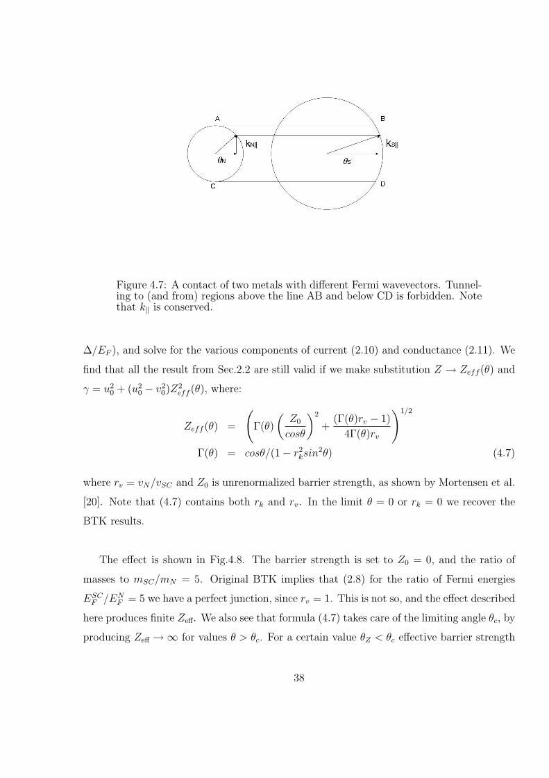
Figure 4.7: A contact of two metals with different Fermi wavevectors. Tunnel-ing to (and from) regions above the line AB and below CD is forbidden. Notethat k‖ is conserved.

∆/EF ), and solve for the various components of current (2.10) and conductance (2.11). We

find that all the result from Sec.2.2 are still valid if we make substitution Z → Zeff (θ) and

γ = u20 + (u2

0 − v20)Z

2eff (θ), where:

Zeff (θ) =

(Γ(θ)

(Z0

cosθ

)2

+(Γ(θ)rv − 1)

4Γ(θ)rv

)1/2

Γ(θ) = cosθ/(1− r2ksin

2θ) (4.7)

where rv = vN/vSC and Z0 is unrenormalized barrier strength, as shown by Mortensen et al.

[20]. Note that (4.7) contains both rk and rv. In the limit θ = 0 or rk = 0 we recover the

BTK results.

The effect is shown in Fig.4.8. The barrier strength is set to Z0 = 0, and the ratio of

masses to mSC/mN = 5. Original BTK implies that (2.8) for the ratio of Fermi energies

ESCF /EN

F = 5 we have a perfect junction, since rv = 1. This is not so, and the effect described

here produces finite Zeff. We also see that formula (4.7) takes care of the limiting angle θc, by

producing Zeff →∞ for values θ > θc. For a certain value θZ < θc effective barrier strength

38

Figure 4.8: Angle dependence of Zeff for Z0 = 0, m1/m2 = 5 and values ofEF1/EF2, from the bottom curve: 2, 1, 1/2, 1/5, 1/8, 1/10.

is Z = 0. At that angle perpendicular components of Fermi velocity are equal:

vN⊥/vSC⊥ = 1 ⇒ tan2 θZ =r2v − 1

1− r2k

(4.8)

Clearly, not all combinations of rk and rv allow the occurrence of a zero-barrier angle. Intu-

itively this minimum corresponds to the increased density of target states corresponding to

the tangential direction on the Fermi surface right before the critical angle is reached.

We will now extend the calculation of Mortensen et al. [20] to include the effects of

anisotropy of a Fermi surface. It should be noted that anisotropic Fermi surface even in

the simplest extension of BTK (i.e.not taking into account the effect of bending of the tra-

jectories (4.6)) produces conductance graphs different from the original, one-dimensional

problem. Since particles incoming at two angles have different Fermi velocity mismatches,

their corresponding Zeff are not equal. They produce different BTK contributions to overall

conductance. However, summing them will not result in BTK-graph, since sum of BTK

graphs for different Z will not produce another BTK graph.

We model a Fermi surface by an ellipsoid, with three principal axis (x, y, z) and the

39

corresponding effective massesmx,my,mz. And let’s say thatmz is large, andmx = my ≈ m.

We’ll parametrize this situation by the angle dependent effective mass m1(θ) = m+δm cos θ.

The other side of the junction is an ordinary isotropic metal with the effective mass m2 = m.

We’ll assume that these functions are known, as well as the Fermi energies on each side

EF1, EF2. We need not worry about which metal is SC and which is N, since equations are

automatically symmetric, so we’ll just call them 1 and 2. We have to take into account

the mismatch of Fermi wave vectors kF1/kF2 and Fermi velocities vF1/vF2 in an anisotropic

system. The problem is that we cannot use the relation (4.6), since rk = rk(θ), as well.

Instead we have:

m1(θ1)EF1 sin2 θ1 = m2(θ2)EF2 sin2 θ2 (4.9)

we can find θ2 solving this equation numerically, and with that value find:

rv(θ1) =v1(θ1)

v2(θ2)=

√EF1

EF2

√m2(θ2)

m1(θ1)

rk(θ1) =k1(θ1)

k2(θ2)=

√EF1

EF2

√m1(θ1)

m2(θ2)(4.10)

Using these values we can find Zeff(θ1) for each incoming angle using (2.8) and (4.7). Note

that even in an anisotropic system:

rv(θ1)rk(θ1) =EF1

EF2

(4.11)

With respect to the large angle scattering events, depending on the ratio of Fermi mo-

menta, there are two possibilities for the geometry of this junction, given in Fig.4.7. A

situation with isotropic kF1 smaller than k2‖ is not interesting, since only particles that are

allowed to tunnel are those with large mass and incident angle close to perpendicular. In

the opposite case these events are allowed, but as we shall now see, strongly suppressed.

To avoid cluttering of the data, the results of this calculation are shown in two figures

- Fig.4.9 and Fig.4.10, for various values of EF1/EF2. These two figures correspond to two

different regimes, similar to k1 < k2 and k1 > k2 in the isotropic case. We see that there

is an expected effect of limiting angle sin θc = 1/rk, and that Zeff grows at large angles.

Thus, despite the fact that large angles are expected to be an easy tunneling direction due

to a good matching of the effective masses and the Fermi velocities for EF1/EF2 = 1, this

40

Figure 4.9: Zeff as a function of incident angle, for a system with m1/m2 =(1 + 4 cos θ) and ratio EF1/EF2 (from the left): 20, 10, 5, 3, 2.5, 2.

does not happen, since conservation of the parallel momentum dictates that this is valid in a

negligible portion of phase space. Even the small variation from π/2 in incident momentum

vector, causes a large difference in perpendicular component of the velocity (since two Fermi

surfaces are tangential to each other), and therefore large Zeff. In comparison with Fig.4.8 we

see that minimum in effective barrier strength occurs not for the combination of parameters

that limits the tunneling angle, but rather for a case where whole Fermi surface is allowed to

tunnel. This is no surprise - the critical angle θc is determined by rk only, whereas the zero

barrier strength is determined by both rk and rv (4.8), thus all combinations are allowed.

The overall effect of this correction is that Zeff (θ) gets larger than Z as defined by original

BTK as we go away from the perpendicular incidence. Consequently, total conductance

(integrated over half-space incident angles) is smaller than it would be calculated by applying

BTK with constant Z at all angles. This is particularly important since (by phase-space

argument) it is tunneling at the incident angles close to π/4 that dominates the transport

in three-dimensional contact junction. The effects can be seen in Fig. 4.11, where correction

is included in the dotted line plot, and pure BTK is given by the full line: tunneling is

suppressed both below and above the gap. The point here is that calculated conductance

cannot be fitted by any value of Z, this curve does not belong to the family of curves

41

Figure 4.10: Zeff as a function of incident angle, for a system with m1/m2 =(1 + 4 cos θ) and ratio EF1/EF2 (from the left): 2, 1, 1/2, 1/5, 1/10, 1/20.

produced by BTK.

As already stressed, equation (4.7) and numerical result for the anisotropic case based on

it are valid only in the limit k+ = k− = kF , which we emphatically want to avoid. Including

this correction is already improvement on existing calculations, but it’s not yet up to the

accuracy we are aiming for.

The problem of finding a refraction angle of the transmitted particle without making

k = kF assumption is easily solved in analogy with (4.9), and for the anisotropic system we

have:

m1(θ1)

(EF1 +

√E2 −∆2

1

)sin2 θ1 = m2(θ2)

(EF2 +

√E2 −∆2

2

)sin2 θ2 (4.12)

which is easy to solve numerically. This equation is interesting, because it shows that in the

limit of two isotropic systems in contact, with slowly varying gap we have:

sin2 θ1

sin2 θ2

=EF +

√E2 −∆2

1

EF +√E2 −∆2

2

=

(k+

1

k+2

)2

⇒

sin θ1

sin θ2

=k+

1

k+2

(4.13)

which is of course Snell’s law. What is interesting is that it shows that even for two perfectly

42

Figure 4.11: Effect of the proper inclusion of the angle dependent Z, for asystem with Z0 = 0.1, rk = 2/3. Dots: calculation with correction taken intoaccount; full line - BTK calculated with corresponding Zeff = 0.367.

matching samples, a particle incoming at an finite angle θ1 slowly bends as it goes from N

to SC. Obviously, the order of this effect is δk⊥/kF⊥ = ∆/EF and it is therefore neglected

in the BTK treatment.

43

4.4 Corrections Not Taken into Account

A few comments are due about the corrections we will not take into account here.

• The effect of a finite lifetime of a particle. This is most often used additional parameter

for the BTK fits. It is application of Dynes’ prescription [26] of substitution of energy

E in teh conductance formulas with E + iΓ, where Γ is inverse quasiparticle lifetime.

Inelastic effects at the interface [27] come as another guise of this correction.

• A finite thickness of the barrier. This is an effect that can be very interesting, since

barrier of a finite width is selective in energy and tunneling angle [22]. However, it

does require an additional fitting parameter, and thus doesn’t fall under the scope of

the corrections we are dealing with here.

• A finite length scale of effective mass onset. Besides the additional parameter, it is

very unlikely to occur in the majoroty of physical systems. For an ordinary BTK our

calculations ([28]) showed that this effect only renormalized Z. This is not surprising,

since slow growth of the mass is equivalent to a change of Fermi velocities. Piece by

piece constant increase of velocity just adds small barriers according to (2.8), but it’s

not so clear how would it affect the full self-consistent calculation.

• Boundary conditions for particles in a band. BTK deals with free electrons, and wave

functions with the wave vector kF , yet it uses an effective mass (band mass), which is

explicitly concept related to a particle in band. As such, it does not describe a wave

function itself, but rather an envelope multiplying rapidly varying Bloch function. This

form of solution is not even well defined at discontinuity, and certainly isn’t continuous.

It has to satisfy only generalized boundary conditions of the form [30, 31] (for time-

reversal invariant system): ψL

∂zψL

a b

c d

=

ψR

∂zψR

(4.14)

where a, b, c and d are real and satisfy unitarity condition ad − cb = 1. They can be

calculated microscopically in a few cases of semiconductor junctions. Our attempts to

see the effect of this change in a simple BTK, showed that any choice of parameters

that satisfies the unitarity condition only renormalizes Z. As if instead three degrees

44

of freedom we had only one. This is likely so because BTK makes ansatz that all

particles are plane waves. This need not be true for a more accurate calculation

with self-consistent gap, where wave functions actually fall off over the length scale

ξ. Question of the boundary conditions and effective masses is also neglected in all

self-consistent calculations, and stays as open and potentially important problem.

• Self-consistent treatment of a condensate. Upon Andreev reflection, pair of electrons

is transfered to a condensate and carried away. Condensate current implies gradient

of a phase, as shown by DeGennes [7]:

∆ = |∆| exp(i2qr) (4.15)

where q is a condensate momentum that has to be determined self-consistently. This

form of the gap in BdG (2.1) in turn produces ’Doppler shift’ - change of energy

of particle with momentum k depending on a direction of motion with respect to

condensate wavevector q:

E = ±

√(h2k2

2m− EF

)2

+ ∆2 +h2

mqk (4.16)

Since in BTK we label the particles by their energy, this produces different momenta

for the particles moving ’left’ and ’right’, and therefore their reflection coefficients.

Obviously, self consistence plays crucial role. However, this task is enormously difficult,

since one has to compute both functional form of the amplitude of a gap and of the

phase. The problem is not yet solved in general, though the calculation with fixed

step-function gap is attempted by Sols and Sanchez-Canizares [29].

This effect becomes prominent in a situation when a bulk SC is connected to a N

side via thin, long (of the order coherence length) SC constriction, and current is

comparable to the critical current of SC. This case is at the moment not interesting

for us, and it remains an important open problem.

• Note that in order to keep the correction of Sec.4.3 in one-parameter regime, it is

necessary to know independently values of EN,SCF and mN,SC , since they enter the

expressions independently through both rk and rv, not only the rv as in the original

BTK (2.8). These quantities can be found by independent measurements, and are

assumed to be known. There is a problem with the nature of the effective mass that

45

enters these expressions - since we are operating with currents, it should be the ’current

mass’ in sense of Landau Fermi liquid theory that enters these expressions. That can

in principle be very different from the effective mass as measured by the specific heat

experiments, e.g. Current mass can be deduced from the experiments that measure

coherence length, likeHc2 in SC materials. Since it is often not independently measured

and known, we have to rely on the band-theory calculations or other experiments, that

measure ’fully dressed’ mass. In that sense, this approximation is a true one-parameter

only if the effective mass is not strongly renormalized by the retarded part of electron-

electron interaction, as explained by Deutscher and Nozieres [23].

46

Chapter 5

Calculation of the Conductance

This section discusses the method of calculation of a conductance in NS junction using

approach similar to the BTK. In practice one has to calculate self-consistent gap first, and

use it to calculate conductance. The order of presentation here is reversed. The reason is

that the method for conductance calculation is natural extension of BTK, and it is easy

to follow. The same method will then be used in a more advanced way to calculate gap

self-consistently. Therefore, in this section we will assume that ∆(r) is known, and in the

Sec.6.2 we will develop a method to calculate it. In essence, both sections are version of

calculation on grid, used in various areas of physics - in context of SC systems it was used

to solve the BdG equations (e.g.Hayashi et al [24]) or the time-dependent Ginzburg-Landau

equations [25].

5.1 Particle with Perpendicular Incidence Angle

If we are given functional form of the gap ∆(r), we can calculate the conductance using

generalized BTK scheme. In the spirit of BTK, we assume that parameters of two sides are

known EFN , EFSC ,mN ,mSC , that there is a delta function barrier at the interface, and that

incoming particles cause no change in the system.

For the moment, let’s study only the particle with perpendicular incident angle. Let

us observe the area of size L around the contact on the SC side. We choose L such that

L ∼= mξ(T ), where m is small number (less then 10). It is obvious that one has to choose

47

Figure 5.1: Schematics of approximation of a real potential by a piecewiseconstant model potential.

length of at least L = ξ(T ) in order to observe the effect of the ’full’ gap ∆0. However, in

order to capture the phase change of the wavefunction upon Andreev reflection properly, one

has to take into account part of the wave function that has exponential decay on the SC side

- for the particles with energy E = ∆ the electron-to-hole conversion occurs at distance ξ(T )

from the boundary, and decay takes another ξ(T ) from the conversion point, thus factor m

has to be larger than 2; it turns out that m = 5, 6 captures all the interesting features and

isn’t wasteful on calculational time.

We then divide the region into n parts of equal length such that ξ(T ) L/n > 1/kf .

Let us call the width of each segment l = L/n. The coordinate of the segment boundaries

are z1 for the contact between N and SC, z2, z3 · · · zn. It is not necessary that all segments

are equal, but it’s very convenient for the implementation in the computer code. Assuming

slow variations of the gap on the length scale l, we make an approximation that gap is piece-

by-piece constant in each segment. Thus for segment i: ∆(r ∈ [zi, zi+1)) = ∆(zi +zi+1)/2) =

∆i = const. See Fig.5.1 for the general idea.

The test of the accuracy of this method on a simple quantum-mechanical system with

known exact solution is given in Appendix A.

With this approximation we can solve separately the BdG equations in each segment

(we get the solution for the homogeneous SC), and match the boundary conditions between

48

the contiguous segments. Following the scattering approach to the problem, we assume a

particle entering from the N-side (left), and there are only outgoing particles on the far right

side (inside SC). However, unlike the original BTK, in all the other segments we have all

four types of the quasiparticles, for i-th segment their amplitudes are (see Fig.5.2):

• - a right-going electron-like quasiparticle (eR): Ai

• - a right-going hole-like quasiparticle (hR): Bi

• - a left-going electron-like quasiparticle (eL): Ci

• - a left-going hole-like quasiparticle (hL): Di.

Thus wave function in segment i is:

Ψi = AiψeRi +Biψ

hRi + Ciψ

eLi +Diψ

hLi (5.1)

where ψ are given by the BdG solutions:

ψeRi =

ui

vi

eiq+i zi ; ψhR

i =

vi

ui

e−iq−i xi (5.2)

ψeLi =

ui

vi

e−iq+i zi ; ψhL

i =

vi

ui

eiq−i zi

For the boundary between i-th and i+1-th segment we have (for i, i+1 6= 1, n) as usual:

Ψi(zi+1) = Ψi+1(zi+1) (5.3)

h2/2mi∂zΨi(zi+1)− h2/2mi+1∂zΨi+1(zi+1) = H ∗ δ1,iΨi(zi+1) (5.4)

where H is unrenormalized delta-function potential, as before; in this case it is present only

at the contact, though the algorithm is applicable to the case of many barriers, as well. For

49

Figure 5.2: One segment with corresponding particle amplitudes.

our case we these conditions read (for i 6= 1):

Ai

ui

vi

eiq+i zi + Bi

vi

ui

e−iq−i zi + Ci

ui

vi

e−iq+i zi + Di

vi

ui

eiq−i zi = (5.5)

Ai+1

ui+1

vi+1

eiq+i+1zi + Bi+1

vi+1

ui+1

e−iq−i+1zi +

Ci+1

ui+1

vi+1

e−iq+i+1zi + Di+1

vi+1

ui+1

eiq−i+1zi

for the continuity condition of the wave function. This is same as (2.6), but now we have

all four types of particles on each side of the boundary. For the continuity of the derivative,

equivalent to 2.7:

Aiiq+i

ui

vi

eiq+i zi −Biiq

−i

vi

ui

e−iq−i zi − Ciiq+i

ui

vi

e−iq+i zi +Diiq

−i

vi

ui

e−iq−i zi =

Ai+1iq+i+1

ui+1

vi+1

eiq+i+1zi −Bi+1iq

−i+1

vi+1

ui+1

e−iq−i+1zi −

Ci+1iq+i+1

ui+1

vi+1

e−iq+i+1zi +Di+1iq

−i+1

vi+1

ui+1

eiq−i+1zi (5.6)

If i = n, the above equations are still valid, but since we have only outgoing particles on

50

the right side, we have to set Cn+1 = Dn+1 = 0 (particle incoming from the left, produces

outgoing particles on the right side).

For the first boundary, we have an incoming particle form the left with amplitude A1 = 1,

and no incoming hole, thus B1 = 0. Also, we have to take into account existence of the

δ-function barrier. Since segment 1 is just the normal metal, we have u1 = 1, v1 = 0.

Altogether, for the wavefunction continuity: 1

0

eiq+1 z1 + C1

1

0

e−iq+1 z1 +D1

0

1

eiq−1 z1 = (5.7)

A2

u2

v2

eiq+2 z1 +B2

v2

u2

e−iq−2 z1 + C2

u2

v2

e−iq+2 z1 +D2

v2

u2

eiq−2 z1

For the boundary condition for derivatives we have (taking into account δ-function bar-

rier):

mSC

mN

iq+1

1

0

eiq+i zi − C1iq

+1

1

0

e−iq+1 z1 +D1iq

−1

0

1

e−iq−1 z1− (5.8)

A2iq+2

u2

v2

eiq+2 z1

+B2iq−2

v2

u2

e−iq−2 z1 +

C2iq+2

u2

v2

e−iq+2 z1 −D2iq

−2

v2

u2

eiq−2 z1 =

2mSC

h2 H

1

0

eiq+1 z1+ C1

1

0

e−iq+1 z1 +D1

0

1

eiq−1 z1

Note that H is unrenormalized barrier strength. This closes the system of 4 ∗ (n + 1)

scalar equations with 4∗(n+1) unknowns (C1, D1, An+1, Bn+1 and Ai, Bi, Ci, Di for i = 2, n).

Casting the system into canonical form (unknowns on the LHS, free-terms on the RHS), we

find the solution by using elementary linear algebra, solving for matrix equation:

M ~A = ~B (5.9)

Where we get M by reading off the coefficients in front of the unknowns C1, D1, A2, B2, C2 . . .,

~A is the solutions vector ~A = (C1, D1, A2, B2, C2 · · ·An+1, Bn+1)T . ~B is given by the incoming

51

particle wavefunction ~B = (−1, 0,−iq1, 0, 0, 0...)T . Similar matrix equation is written out

explicitly in Appendix A.

In order to calculate conductance, we actually need only the terms on the far left and far

right side, thus C1, D1, An+1 and Bn+1. For the particle incoming from the N-side they have

the obvious physical meaning:

• - C1 - an amplitude for the specular reflection

• - D1 - an amplitude for the Andreev reflection

• - An+1 - an amplitude for the transmission without branch-crossing

• - Bn+1 - an amplitude for the transmission with branch-crossing.

Since the total probability is conserved, the following condition is satisfied:

|C1|2 + |D1|2 ∗k−1k+

1

+ (|An+1|2 ∗k+

n+1

k+1

− |Bn+1|2 ∗k−n+1

k+1

)mN

mSC

(u2n+1 − v2

n+1) = 1 (5.10)

similar to the corresponding condition in the original BTK. Additional condition is satisfied

on the boundaries between the segments, also corresponding to the conservation of current.

Ji(zi) = Ji+1(zi) ⇒ Im (Ψi(zi)∇Ψ∗i (zi)) = Im

(Ψi+1(zi)∇Ψ∗

i+1(zi))⇒

(k+i |Ai|2 − k−i |Bi|2 + k+

i |Ci|2 − k−i |Bi|2)(u2i − v2

i ) =

(k+i+1 |Ai+1|2 − k−i+1 |Bi+1|2 + k+

i+1 |Ci+1|2 − k−i+1 |Bi+1|2)(u2i+1 − v2

i+1) (5.11)

Though not of direct use for calculating the observable quantities, Eq.(5.11) is an excellent

tool for checking for the systematic errors in calculation, and is used throughout the present

work.

Finally, the conductance for the single quasiclassical trajectory is given by:

σN−SC = 1 + |D1|2 ∗k−1k+

1

− |C1|2 . (5.12)

To get a conductance at a finite temperature, we employ a small trick and the equation

(2.16). We first calculate profile of ∆(r;T ) for a given T . Then for that profile we calculate

σ(E) from (2.16) (i.e.conductance that would result from a given profile at T = 0, and

which in itself is not a measurable quantity), and using (2.16) we get a self-consistent finite-

temperature conductance, which is measured in the experiments .

52

Already at this point we can get some interesting results. Let us put step function for

a gap profile ∆(r) = ∆ ∗ θ(z − z1), and say that potential barrier is Z = 0. Results of our

calculation should then coincide with the analytic BTK solution. That indeed is the case,

only if we make BTK approximation and set k+ = k− = kF ! E.g. for the components of the

current our graphs fall right on the top of those in Fig.2.5. However, keeping the momenta

exact, makes qualitative change. Results of this calculation are shown in Fig.5.3. Note that

coefficients a and d are not zero, compared to results shown in Fig.2.5. Retaining the exact

momenta enables a particle to be specularly reflected and transmitted with branch crossing

even without interface barrier.

Reason for this is the non-exact matching of say incoming k+ from the N side, and cor-

responding k+ on the SC side. Difference of these wavevectors results in a different particle

velocities. Effect of non-matching velocities is similar to (2.8), in a sense that system be-

haves as if there were a barrier. Particularly interesting is an observation that probability for

the transmission with branch crossing d grows with energy, very different from the behavior

of BTK system with barrier (Fig.2.6), where this coefficients falls off rapidly as energy is

increased. Reason for this is that as energy is increased the difference between wave vectors

k+ and −k− gets smaller, and transition to a hole branch gets easier. The effect is very

small, though, and we can see in Fig.5.3 that even for an extreme case ∆/EF = 0.2, branch

crossing and specularly reflection terms carry only 2% of the total current.

Using this method we can also see how is current distributed among the four types of

particles in the space, as shown in Fig.5.4. Electron is incoming from the right, and since

it has E < ∆ exponentially falls off to the right. Same happens with transmitted hole.

Electron and hole going to the right (specularly and Andreev reflected) have components

only on the right side. At some point there is no more current carried by the quasiparticles,

all current is carried by the condensate.

It is not hard to determine the fall-off length. E.g. for an incoming electron with zero

energy, we have:

k+ =

√2m/h2

√E2

F + i∆ ≈√

2mEF/h2 (1 + i∆/2EF ) (5.13)

and it is the imaginary part that produces the suppression of a wave function through

53

Figure 5.3: Components of the conductance for a system with step-functiongap and exact momenta retained throughout the calculation, with Z = 0,µ = 1eV , ∆ = 0.2eV (upper row): a-transmission without branch crossing,b - transmission with branch crossing, (lower row) c - Andreev reflection, d-specular reflection. Note a different scale in parts c and d. Compare withFig.2.5 to see an effect of exact momenta. Vertical axes - current, normalizedto the incoming particle; horizontal axes - energy, in units 0.1meV

54

Figure 5.4: Distribution of the current in space for each component eR, eL(upper row), hR, hL (lower row), normalized to the incoming eR current.Z = 0.7, µ = 1eV , ∆ = 0.1eV . An electron is incoming from the right,position of the barrier is at the mark 50. Length ξ is 10 divisions on x axis.

55

exp(ik+r) term, with factor exp(−∆kF/2EF ). The suppression factor for a current is square

of this term, and we get for a distance at which current falls off to 1/e of its original value:

r1/e(E = 0) = EF/∆kF = h2kF/2m∆ = π/2 ∗ ξ (5.14)

Thus current of a particle at E = 0 penetrated into the SC to a distance of the order ξ. For

particle with energy that is a fraction α of the gap - E = α∆:

r1/e(E = α∆) = EF/∆kF = h2kF/2m∆ = π/2 ∗ 1/(1− α2) ∗ ξ (5.15)

which can be much larger than correlation length ξ.

5.2 Finite Incidence Angle

It looks as if it were easy to apply the procedure given above to the arbitrary angle. Since the

incoming particle ’sees’ longer effective onset length, one way to do it is to simply rescale all

the lengths by the factor 1/cosθ, where θ is angle of incidence, measured from the direction

perpendicular to the interface, and weigh each trajectory by cosθ (since only perpendicular

component of the current contributes to the conductance). The weighing factor for a con-

tribution from angle θ in three-dimensional sample is 2π sin θ ∗ cos θ, where 2π sin θ is the

phase space factor, and cosθ is a fraction that contributes to the conductance. We see that

this factor has maximum when θ = π/4, thus in isotropic three dimensional sample particles

incoming at the intermediate angles dominate the transport.

We have to be careful with this approach, since we are not solving the equations along

the direction of motion. Procedure has to conform to the symmetry of the problem, so we

shall separate the parallel and the perpendicular components, and apply algorithm from the

previous section to a perpendicular component only. Since we are solving BdG equations

(2.1) separately in each segment, we get solutions of the form (2.2), as in previous section.

The difference is that now we ought to take care of the phase accumulated by a parallel

56

component. Solutions are of the form:

ψeR =

u0

v0

eiq+ cos θ∗zeiq+ sin θ∗ρ;ψeL =

u0

v0

e−iq+ cos θ∗ze−iq+ sin θ∗ρ (5.16)

ψhR =

v0

u0

e−iq− cos θ∗ze−iq− sin θ∗ρ;ψhL =

v0

u0

eiq− cos θ∗zeiq− sin θ∗ρ

where ρ is coordinate in x, y plane, parallel to the interface and perpendicular to the direction

of motion, and from the geometry of the problem ρ = z tan θ. Then we can rewrite this

equation (using cos2 θ + sin2 θ = 1) as:

ψeR =

u0

v0

eiq+z/ cos θ;ψeL =

u0

v0

e−iq+z/ cos θ (5.17)

ψhR =

v0

u0

e−iq−z/ cos θ;ψhL =

v0

u0

eiq−z/ cos θ

Thus the result is identical to a ’naive’ one, and the overall effect is that length scale is

rescaled by cos θ−1.

However, we have already seen in Sec.4.2 that incident angle of electron and hole are not

identical for finite energy and θ > 0. Thus, strictly speaking, the wave functions are:

ψeR =

u0

v0

eiq+z/ cos θ+

;ψeL =

u0

v0

e−iq+z/ cos θ+

(5.18)

ψhR =

v0

u0

e−iq−z/ cos θ− ;ψhL =

v0

u0

eiq−z/ cos θ−

where θ+ and θ− refer to an angle of incidence of electron and hole, and they are related

by equation (4.3). This equation takes care of NERR effects. For every segment, starting

from the known energy E and the incidence angle θ+ of an incoming electron, we calculate

the angle θ− for a hole. If θ+ > θ0 given by (4.4), angle θ− becomes complex. Then we

define coefficients in (5.18) so that the entire term is exponentially suppressed when θ− is

complex (this has to be done by hand, since making cos θ− with complex θ sometimes makes

exploding solution either for ψhL or for ψhR). This still allows particle to be transmitted, if

it has enough energy, but cannot AR.

57

Figure 5.5: Schematics of the change of incident angle for a sequence of seg-ments, due to the increase of gap at the barrier, as calculated in (4.12)

.

Next question is how shall we incorporate results derived in Sec.4.3 without dropping out

terms of the order ∆/EF , as we had to do to derive explicit formula (4.7). The beauty of

this approach is that we don’t have to calculate Zeff at all! What are we really doing here is

solving the system of the equations (5.5, 5.6...) with exact momenta retained in all terms.

In that sense, we do not need to reduce the problem to a single mass m, or momentum kF ,

all terms can be kept just like they are, without any renormalization of the barrier strength.

Only Z that enters the problem is Z0 - given by unrenormalized δ-potential, without contri-

butions from Fermi velocity mismatch etc. The problem of finding angle θi for each segment

is solved in (4.12).

Thus the procedure is following: for every given energy and the incident angle for an in-

coming electron θ+1 , we calculate the propagation angle in subsequent segment using (4.12).

Now having a set θ+i for every i, we can use (4.3) to calculate angle for the hole θ−i in each

segment. We suppress hole wave function in segment i if θi > π/2. Now we have set of

wave functions (5.18), which we plug into the procedure for perpendicular incidence given

in Sec.5.1. We solve the system of equations as described, with unrenormalized Z as barrier

strength. For every energy we run the loop over all angles θ, with weight factor 2π sin θ cos θ

and we automatically get conductance with effects of finite angle incidence, NERR and exact

58

momenta accurate in the order ∆/EF (thus, making error of the order (∆/EF )2)...provided

that we had accurate ∆(z) to start with.

By doing this, we have applied all the corrections mentioned in Sec.4, except self-

consistent gap calculation ∆(z). That is a subject of the following section.

59

Chapter 6

Self-consistent Gap Calculation

Important effect that one has to include in the conductance calculations is that of the fi-

nite length scale. While any functional form of ∆(r) can be plugged into the calculation

scheme for the conductance in Sec.(5.1), to get the correct answer we have to use one that is

obtained self-consistently with the same parameters that we use for the conductance calcula-

tion - Fermi energies (ESCF , EN

F ) and effective masses (mSC ,mN) on two sides of the junction,

bulk gap value ∆0 and temperature T and Z. E.g., electrons that we shoot in to test for

conductance have to see same barrier as those in the SC that determine shape of the gap.

All calculations of this kind so far have been done either non-self consistently or in quasi-

classical limit. The self-consistent calculation presented here does not make the quasiclassical

approximation, and as such is valid even in the limit when ∆/EF is not small. Also, it does

not rely on Green function approach, and therefore does not suffer of the problem of ’ex-

ploding solutions’, common to quasiclassical calculations - this solution is given entirely in

terms of wave functions. The fact that only basic formulas (2.1) are used gives it appealing

simplicity. The wavefunctions of the system are calculated numerically, and ∆(r) obtained

from the definition (2.1). The approximation that we do make is that ∆(r) varies slowly

over the range l = L/n (except at the barrier itself), and can be taken to be constant in a

segment of the width l (n is a number of segments, L total length of the region around the

interface that we study). The accuracy of this approximation will be discussed later.

Whatever our approach, the final aim is to calculate functional form ∆(r). Appendix C

60

summarizes the definition and various equations one can use for this calculation. We can

get ∆(r) either by knowing the off-diagonal component of the quasiclassical SC propagator,

or by knowing the wave-functions of the BdG or Andreev eigenproblem.

6.1 Quasi-classical Self-consistent Gap Calculations

To understand the advantages of our approach, let us first look into the standard, quasi-

classical calculation. The first attempt along these lines was made by McMillan [32], who

considered the SN contact without the barrier, and did one-loop approximation, effectively

ending iterative self-consistent process after first iteration. McMillan used Andreev approxi-

mation, but didn’t use the Eilenberger quasiclassical Green function formalism. Eilenberger

[33] and Larkin and Ovchinnikov [34] formulated the equations of motion for the quasiclas-

sical propagator. These equations are supplemented by the various boundary conditions in

works of Buchholtz and Rainer [35] for a surface wall, Zaitsev [36] for a contact between

two metals, Millis et al. [37] for a magnetically active interface, and later in their work by

Ashauer et al. [38] for a non-conventional SC, and Fenton [41] for the heavy fermions. The

application of the formalism to the study of 3He was done by Serene and Rainer[40]. Zhang

et al. [42] calculated ∆(r) for two semi-infinite slabs in 3He, and Kieselmann [39] for the case

of finite N layer touching the bulk SC. Nagai and Hara [43] found the proper normalization

for the contact of two finite slabs, which is applied to calculate ∆(r) in bilayer by Ashida

et al [44] and Hara et al [45], and tri-layer by Nagato [46]. Anisotropic SC are studied by

Bruder [47], and zero-bias states (and their splitting) are found self-consistently by many

groups, e.g. Matsumoto and Shiba [48], Fogelstrom et al [49], Barash et al [50] etc.

The starting point of all these calculations is linearization of the energy spectrum around

the Fermi surface. By making the following ansatz in BdG equations:

un(r, t) = un(r) ∗ exp (−i(E ∗ t− kF nr) (6.1)

vn(r, t) = vn(r) ∗ exp (−i(E ∗ t− kF nr)

we factor out the x, y dependence and fast oscillating part of the wave function in the

direction of motion of particle (or other, dictated by symmetry of the problem), and by

61

neglecting terms in BdG of the order h2/2m ∗ (k − kF )2/EF =√E2 −∆2/EF ≈ ∆/EF we

get the linearized BdG, also called Andreev equations:

Enun(r) =

(−ihvF

∂

∂r

)un(r) + ∆(r)vn(r) (6.2)

Envn(r) = −(−ihvF

∂

∂r

)vn(r) + ∆(r)un(r)

As usual, problem can be discussed in terms of the wave-functions only, or in terms of

the Green functions. If we apply the same approximation to the Green functions in Gorkov’s

equations, we’d get their quasiclassical equivalent - the Eilenberger equations. The basic

formulas concerning these are given in Appendix B. Since Eilenberger equations provide

a condensed way to write sum over the states, they are the main tool in the quasiclassical

study of NS contacts. As shown in AppendixC, we can use either approach to calculate ∆(r).

Compared to the original BdG system, equations(6.2) have a great advantage that they

are the first order differential equations, and thus very easy to solve numerically. Of course,

they have to be supplemented by the boundary conditions. For a moment we’ll consider two

semiinfinite slabs with the same parameters (Ef ,m), the only difference between them being

that one is SC and another N. In that case, un and vn at ±∞ are given by their bulk SC and

bulk N values. The problem that remains is how to match them at the boundary. By making

Andreev approximation, we integrated out the short length scale degrees of freedom (of the

order 1/kF ), so the continuity equations valid for the BdG wave functions do not apply

here. We can find proper boundary conditions by studying the reflection and transmission

coefficients for the current carried by a particle of given energy. The boundary is described

by the behavior of an incoming particle at Fermi surface:

ψ1 =

e−ik1zz + reik1zz ; z > 0

te−ik2z ; z < 0;ψ2 =

eik2zz + re−ik2zz ; z < 0

teik1z ; z > 0(6.3)

For the case that we consider r =√R, t =

√1−R, and R is the reflection coefficient

at the interface, parametrized by the BTK parameter Z as R = Z2/(1 + Z2). We then use

these equations and the continuity of the exact wave function (un, vn) to find the boundary

conditions for a slowly varying part (un, vn), controlled by the Andreev equation.

62

Zaitsev [36] has applied this alghoritm to study the properties of various components of

the Eilenberger propagator. He observed the part of the propagator constructed by two left-

going (g−−) and two right-going (g++) particles (see AppendixB and the following section)

and derived the boundary conditions satisfied by odd and even components of the propagator

with respect to the contact. One can therefore solve the Eilenberger equations numerically

starting from, say, known bulk value of the propagator, with the boundary conditions given

in AppendixB. This is approach used by, e.g. Kieselmann [39] or Bruder [47].

Another approach is pursued by the Japanese groups. They study the asymptotic behav-

ior of the wave-function solution of (6.2), and construct an evolution operator that transforms

the solution along the coordinate axis. From these solutions they construct the Eilenberger

propagator, which automatically satisfies the boundary conditions [45].

Either way, one has to start, with calculations far on the superconducting side, where all

the variables have known, bulk superconducting values, then calculate the derivative from

(6.2) and use that derivative to calculate values at the next step (this is in essence Runge-

Kutta method for numerical solution of differential equation). At the contact, the value at

the SC side will be known, and from the boundary conditions we can calculate the value at

the N side, and continue with the calculation. From thus obtained wave-function/Green func-

tion, we can calculate a new ∆(r) and repeat the calculation until convergence is achieved.

At this point it is obvious why the method needed modification [43] for the finite SN

slabs: if width of the SC slab dSC is of the order ξ or smaller, the gap never achieves the

bulk value, and we don’t know from the outset how to normalize the calculation (i.e. the

starting value is not known). Rather, normalization has to be determined in the iterative

process itself.

The overall accuracy of this approach is limited by the approximation made in the first

step - neglecting the term (k − kF )2 implies that the energy is calculated with the accuracy

of ∆/EF . Also, quasiclassical particles are allowed to live only on their trajectories, and

effects of NERR are neglected, as well as the effects related to the finite incidence angle

63

we discussed in Sec.5.2. The improved method we will now present takes care of all these

drawbacks, in much the same way we did in sections 5.1 and 5.2.

6.2 Improvement on Quasiclassical Approach

One obvious problem with using quasiclassical gap, is that aim of our conductance calculation

in a first place is to include the corrections of the order ∆/EF . As stressed before, quasiclas-

sical calculation explicitly neglects the terms of this magnitude. In order to be consistent,

we have to keep the terms of this size throughout the calculation. It is also methodologi-

cally interesting problem, since some effects simply cannot be taken into account through

quasiclassical approximation - e.g. drift states due to NERR at the (110) surface of SN

contact of d-wave SC, and thus cannot be taken into account self-consistently in density of

states calculation (drift states may be directly observed in an experiment similar to [51],

though they were not found in that particular work). It was this method that we used for

self-consistent calculations throughout this work. Particular appeal for this choice in study

of the conductance is that exactly the same algorithm is used for both calculations.

Instead of the above described quasiclassical approach, we will make use of the algorithm

described in Section 5.1. We divide the region around the boundary in segments, and as-

sume piecewise constant properties (gap ∆ in particular) in each segment. That enables us

to solve the Bogoliubov de Gennes equation (and not the Andreev equation) exactly in each

segment, and match the boundary conditions between them. The process is equivalent to

that described in the previous section, and will not be repeated. Note that we are match-

ing the boundary conditions of the wave functions, and not envelopes (except in a sense of

comment in Sec.4.4), so we are entitled to use usual boundary conditions of the continuity

of wave function and it’s derivative. We start off with initial guess of ∆(r) which may or

may not be a step function. Our aim is to determine convergent solution ∆(r) in an iterative

process using equation (2.1).

At this point we will not specify which side is is SC and which is N. The entire calculation

is insensitive to the swap, as all the expressions are put in a symmetric form. A N side is

64

Figure 6.1: Boundary conditions for a SN contact: an electron incoming fromthe left (A) and a hole outgoing to the right (B). Full line - electron, dottedline - hole. Arrows point in the direction of propagation. N metal is on theleft side of the interface in both figures.

defined in a same way as SC side, with ∆ = 0 and (consequently) Tc = 0. In that sense,

when we speak of an electron or a hole as an abbreviation for ’electron-like quasiparticle’ or

’hole-like quasiparticle’.

Let us observe an incoming electron from the left (eR) (Fig.6.1, A ). It will propagate

to the boundary, and there either get transmitted or reflected in one of four ways. Note

that there is a finite probability for a transmission to a certain distance even if E < ∆ (see

Fig.5.4). Possible sequence of specular and Andreev reflections is given in Fig.6.2. We see

that in this process we start with pure electron with a wave function in particle-hole space

(1, 0)T , and we end up with a mixture of electron and hole wave-function on every ’branch’

of this process. This is a process that describes transfer N side particles into a SC. Note

that this is exactly the same calculation as the one described in a Sec.5.1 - we shoot electron

from a RHS and calculate it’s wave-function everywhere. The difference is that now we are

not interested in transport properties (i.e. coefficients C1, D1, An+1 and Bn+1), but rather

in the amplitudes of the resulting wavefunctions throughout the system. These amplitudes

were calculated in Sec.5.1, but were not used - they were just intermediate states connecting

65

particles we were interested in (i.e.outgoing particles at the edge of the system).

We also need to include a process that describes transfer of particles from SC to N. We

choose boundary condition of outgoing hole (hR) on the SC side (Fig.6.1, B). Both cases can

be described by a same diagram in Fig.6.2 (left panel). It takes very little modification to

our algorithm from Sec.5.1 to describe wave functions resulting from this boundary condition

(e.g.we can make prescription u ↔ v and k+ ↔ −k− and use the same algorithm). This

process describes transfer of a hole (in this case outgoing) from SC to N metal.

We also need the processes that describe transfer of a hole from N to SC, and an electron

from SC to N. For that we choose outgoing hole on the right (hL) and incoming electron

on the left (eL). These two cases produce diagrams corresponding to Fig.6.2 with all arrows

reversed. They are also calculated easily with prescriptions similar to the algorithm for (hR).

There are also other possible processes, but they are not independent from those described.

Each of these processes results in a wave function of a type (5.1) in each segment. All

we have to do now is to use the self-consistency condition of BdG to calculate the gap:

∆(r) = V Σnfn(r, t)g∗n(r, t) ∗ (1− 2n(En)) (6.4)

Since ∆ exists only on SC side (where V is non-zero), we also define correlation function,

which describes the density of pairs on both SC and N side:

F (r) =∑

n

fng∗n(1− 2n(En)) (6.5)

Sum n runs over all available states. In BdG we have four states for each energy, and those

are the states we described with four boundary conditions (eR, hR, eL, hL). Contribution

to the gap from each of them is added separately. A question left is how to deal with two

intersecting branches of the same wave-function that contribute to the correlation function.

We can either add amplitudes and then make product uv∗ or the other way around. Since

this is one wave function, we really should do the former. However, ’interference’ terms

resulting from such product have the fast oscillating factors of the type exp(i(k+ + k−)) or

exp(2ik±), compared to exp(±i(k+ − k−)) or 1 that we have on a same branch. These fast

66

oscillations get averaged out to zero, and we will not include them (this is also standard

procedure in the quasiclassical theory).

Let us write down explicitly the wave function (f, g)T in segment i:

Ψ =

fi

gi

=

Aiuieik+

i r +Bivie−ik−i r + Ciuie

−ik+i r +Divie

ik−i r

Aivieik+

i r +Biuie−ik−i r + Civie

−ik+i r +Diuie

ik−i r

(6.6)

Summing all the non-fast oscillating terms together we have:

∆(r) = V∑

n,θ,p(1− 2n(En)) (6.7)(ui ∗ Ai ∗ eik+

i r + vi ∗Di ∗ e−ik−i r)(vi ∗ Ai ∗ eik+i r + ui ∗Di ∗ e−ik−i r)∗ +

(vi ∗Bi ∗ eik−i r + ui ∗ Ci ∗ e−ik+i r)(ui ∗Bi ∗ eik−i r + vi ∗ Ci ∗ e−ik+

i r)∗|n,θ,p

where p is counting particles for each state p =eL, eR, hL, hR; the sum now goes over

all positive energy states n and incident angles θ. States with three indices (n, θ, p) are

non-degenerate. Subscript i denotes that functions of r are calculated in the segment at

distance r; r ∈ [i ∗ l, (i+ 1) ∗ l). The notation is same as that of Sec.5.1. Note that u, v,

and k± are all implicit functions of ∆(r) and E. To get actual ∆(r), one has to sum the

contributions from all energies and angles. Exactly the same equation applies to the right

side, with appropriate r and i plugged in. Prefactor V is interaction constant, which we

dispose of by normalizing a gap to the known bulk value far on the SC side.

In drawing Fig.6.1 and Fig.6.2 we pretended that particle specularly reflects only at the

interface. However, as we know from 5.3 if we keep the exact momenta this is not true.

In practice this is not a problem, since algorithm allows mixing of the components of wave

functions at every step.

The results of this calculation are well-known from the quasiclassical approach. Clean

limit contact has a gap that decays on the length scale ξ. At finite temperatures ξ(T ) in-

creases, as consequence of the decrease of ∆(T ).

The presence of barrier disrupts the transport of pairs across the contact, and conse-

quently the fall-off length is shorter then ξ. In the limit Z → ∞ gap stays constant all

the way to the contact. This case is equivalent to the outer surface of SC (’N metal’ is

vacuum), and the result can be explained by the well-known Anderson argument. This goes

67

Figure 6.2: Processes (A) and (B) from the Fig.6.1 drawn to include AR alongthe trajectory (left). Contributions to the gap from two trajectories at everypoint in space (right).

as follows: in s-wave SC, non time reversal breaking impurities (including surfaces) have an

effect of mixing different values of momentum k. This means that k is not a good quantum

number anymore, however, that does not influence the SC properties, since SC Hamiltonian

can be rewritten in terms of new time-reversed states (n, n) instead of the usual (k,−k). In

particular, the gap will not be supressed at such impurities. This is also valid for Z → ∞

case. For finite Z, closer we are to this limit, shorter the gap-onset length.

Although no results by other authors are available to check the application of our method

in the regime ∆/EF ≈ 1, with the choice of parameters appropriate for Nb (EF = 4eV,∆ =

1meV ) the results are in agreement with those of quasiclassical approach (see Fig.6.5).

Following discussion is related to the Nb at T = 0 in contact with isotropic N metal with

same characteristics as Nb.

Fig.6.3 shows the contributions to the pair correlation function (defined by equation (??)

from two different energies. A left figure shows the energy just above the gap. Oscillations

are related to the coherence between electron and a hole, wave length is 2π/(k+ − k−). We

see that it is smaller on the N side - since in SC an electron and a hole just above the gap

have (almost) the same wave vector (see Fig.2.1). Figure on the right side is for energy of

the order 3∆ - electrons and holes in SC are almost decoupled, and interference terms are

68

Figure 6.3: The unnormalized contribution to the pair correlation function(6.5) from the particles of one energy and along one incident angle for Nb,Z=0, T=0 (E ≈ ∆ (left), E ≈ 3∆ (right)). Units on x-axis are 1/10ξ, andcontact is at the mark 100, N is to the left, SC to the right of it.

of the same wave length as in N.

In Fig.6.4 (left) we see the contributions from one angle - θ = 0 integrated over all en-

ergies. The ripples are consequence of electron-hole coherence, and they disappear after we

sum contributions from other angles (right). They are not artifact of the calculation. They

appear because Andreev reflection (the source of electron-hole coherence) occurs in a limited

energy range, and contribution to the pair correlation function from corresponding k+−k− is

dominant. Note that in Fig.6.3, scale along the ’F ’ axis (vertical) is ten times larger for the

particles of smaller energy (two graphs have same normalization, and are thus comparable -

even though they are not normalized with respect to the bulk value of F ).

In Fig.6.5 we have the pair correlation function after three iterations, and the gap cal-

culated from these iterations. The gap value changes somewhat in subsequent iteration, but

the curves are too close to be shown in this figure. A finite temperature calculation is given

in 6.6. To do this calculation we use the transcription of integral with Fermi factor to a sum

over Matsubara frequencies, given in Appendix C. Besides the smaller gap, we see that the

effective correlation length ξ is longer (gap grows to the full value over longer distance). In

Fig.6.7 the same calculation is repeated for barrier with Z = 4. Evidently, there is a jump

in correlation function, and gap offset value (initial jump of gap magnitude) is 0.9∆ (instead

of 0.5∆ for a clean contact).

69

Figure 6.4: The unnormalized contribution to the pair correlation functionfrom particles at an incident angle θ = 0 (left) and integrated over all angles(i.e. after complete first iteration) for Nb, Z=0 (E ≈ ∆ (left), E ≈ 3∆ (right).Units on x-axis are 1/10ξ, and contact is at the mark 100.

Figure 6.5: The calculated gap in each iteration (top to bottom) (right) andthe unnormalized pair correlation function after three iteration loops (left) forNb, Z=0 . Units on x-axis are 1/10ξ, and contact is at the mark 100.

70

Figure 6.6: Self-consistent gap and normalized pair correlation function forT = 0.95Tc, all parameters are the same as in other figures.

Figure 6.7: Self-consistent gap and normalized pair correlation function forbarrier parameter Z = 4.0, T = 0, all parameters the same as in other figures.

71

Figure 6.8: Self consistent gap after 4 iterations for EF = 1eV and ∆ = 0.1eV(left) and ∆ = 0.2eV (right) at T=0, Z=0.

Finally, we show the results in the case when ∆/EF is not small in Fig.6.8. One interesting

feature that we would like to stress is offset value of the gap, which is not 0.5∆ as for other

clean systems, but larger. We saw that large value of gap offset corresponds to the presence

of the barrier (Fig.6.7). The ’barrier’ in this case is a mismatch of wave vectors on N and

SC side due to the large gap, which we already saw to produce an effect similar to finite Z

in Fig.5.3.

.

Let us address the accuracy of the method. As we said above, the quasiclassical method

neglects energy terms of the order ∆/EF . An error that we make using segment model is

of the order (∆/Ef )/n on each segment. Note that for the given boundary conditions (i.e.

solution in the contiguous segments) solution Ψi in the i-th segment is exact - wave function

itself bends to accommodate imposed boundary conditions. For this reason, error in one

segment cannot propagate to other segments, only choice of potential ∆i causes error in

segment i. We see that only if there is a systematic error in choice of potential ∆i, we will

have overall accuracy as big as quasiclassical one. If the choice of potential is ’perfect’ (in a

sense that boundary conditions of a wave function are identical to the exact solution on that

segment for given E), solution is exact in the limit n→∞, and the error propagation is sim-

ilar to the one-dimensional random walk (which is, of course, localized). In a case that there

is a small systematic error in choice of ∆i, this random walk process acquires a drift, and

there is finite error even in the n→∞ limit, although still smaller than the quasiclassical one.

72

Chapter 7

Results and Interpretation

We will now present the results of a fully self-consistent calculation taking into account

the corrections from Sec.4, on a model of a contact junction between highly anisotropic

and isotropic metal. Choice of anisotropy is stipulated by the results of [14]. According

to Deutscher and Nozieres [23] not all the renormalization of electron mass is important

in tunneling, it is also clear that in CeCoIn5 at least part of the anisotropy comes from

lattice structure effects - we choose the numbers so that in the limit of clean contact they

approximately reproduce ZB conductance measured by [14]. We choose model anisotropy as

in Sec.4.3:m1/m2 = 1 + 4 cos θ. Results for the zero-temperature conductance are given in

Fig.7.1.

Conductance plots in Fig.7.1 are compared with the BTK fit that has same value of

high-voltage conductance. We see that plots are not identical to BTK, but they still have

undoubtly BTK features - such as coherence peak and finite subgap conductance. There

is not much difference between the gap onset length scales for these systems - see Fig.7.3

for comparison of the self-consistent gap for systems with ratio of Fermi energies 0.2 and 3.

Thus, most of the differences comes from what in BTK limit (all momenta set to kF ) would

be renormalization of Zeff and NERR.

Let us make a couple of remarks about the results before going to discussion of details. It

is interesting to compare plots of Fig.7.1 and Fig.7.2. We have plots for the ratio of Fermi

energies 2 and 3 given for the same Fermi energy of the N side (1eV) and three different

73

Figure 7.1: Evolution of the conductance curve formSC/mN = (1+4 cos θ) andEFSC/EFN 1/5, 1/2 (upper row), 2, 3 (lower row). EF = 1eV , ∆ = 10meV ,Z0 = 0. Full line is BTK curve, fitted to the high energy values, dotted lineis this calculation. Vertical axis is a conductance, normalized to a perfectcontact, horizontal - energy, in units 1/100∆.

74

Figure 7.2: A conductance curve for mSC/mN = (1 + 4 cos θ) and EFSC/EFN

- 2 (left)and 3 (right) . Z0 = 0, EF = 1eV , ∆ = 100meV (upper row)and ∆ = 200meV (lower row). Full line is BTK curve, fitted to the highenergy values, dotted line is this calculation. Vertical axis is a conductance,normalized to the perfect contact, horizontal - energy, in units 1/100∆.

Figure 7.3: A comparison of the self-consistent calculation of the gap for asystem with mSC/mN = (1 + 4 cos θ) and EFSC/EFN - 0.2 (dots) and 3 (fullline), after four iterations. Vertical axis is gap in eV , horizontal is distance inunits 1/10ξ - contact at 50.

75

values of the gap on SC side - 10meV, 100meV and 200meV. There is a surprisingly little

difference between the plots, and the plots with gap of 10meV and 100meV are almost

identical. Only gap of 20% of Fermi energy bring significant change, mostly due to the

non-matching of various wave-vectors and the effects of NERR. One interesting feature is

that large gap plots have a slight upturn in the conductance as E → 0. This is due to the

mismatch of the momenta, which is smallest at ZB and also due to the NERR, which is

important at finite voltages. As energy increases, the mismatch grows larger, and in a sense

of Fig.5.3 ’an effective barrier’ gets larger. Note that since we do not have a real barrier in

this case, it is not a surprise that there is not much change in the conductance above the gap,

where NERR is not important process - comparing to Fig.5.3 we see that the overal effect

of the mismatch of the momentum vectors is very small, and that current above the gap is

also carried by a branch-crossing process. Also, as the gap increases, the coherence length

gets smaller, and so the effect of the finite length-scale in a system becomes less important.

It is the ratio of conductance at E < ∆ and E ∆ that is to some extent non-BTK like,

and that can be explained by a finite length-scale effects, which we will now discuss.

7.1 Effects of Finite Gap Onset Length

As expected in analogy with the quantum-mechanical ramp potential, and as discussed in the

connection with Fig.4.2, the finite gap onset length combined with the momentum mismatch

leads to the suppressed excess conductance above the gap. This effect is more prominent

with the longer gap onset length, which is of the order L ≈ ξ. On the other hand, L ≈ ξ is

inversely proportional to ∆. A momentum-mismatch on two sides, which also reduces the

conductance, is proportional to ∆ (for small ∆, at least). Thus only one of these two effects

can be large.

A self-consistent calculation limits the size of ξ. This restricts a behavior very different

from the BTK to the quasiclassical trajectories at very large incident angles (with effective

L(θ) = L/cos(θ) ξ). However those particles carry a small perpendicular component of

momentum, and have a little influence on the overall tunneling characteristic (integrated

over all angles).

76

Figure 7.4: Evolution of the subgap structure with incident angle, Z=1.3,Ef = 1eV , ∆ = 1meV : full line - BTK, dots - this calculation, normalized sothat conductance at high voltage without barrier is σ0 = 1. Consequence ofthis normalization is that subgap conductance σSN(E) = 2 means that particleat that energy does not feel the presence of the barrier.

We have seen both in Fig.4.2 and in Fig.7.1, that there is a slight shift of a maximum

conductance from the gap edge to the values of energy E < ∆, accompanied with the

enhanced subgap conductance (compared to the BTK), as if gap were ’filling up’. To see

why this happens, let us isolate the effect of the trajectories at very large incidence angles.

Fig.7.4 shows the sequence of the trajectories incoming at a large angle. In this calculation,

to make the effect more prominent, we did not use the self-consistently calculated gap (it

will be clear later why - it tends to suppress the effect we are to demonstrate). Instead, we

use Ginzbug-Landau form. We see that maximum is shifted more as the angle, and thus

the effective length L/cosθ increases. The conventional interpretation of that effect is that

quasiparticles probe only the length-scale ξ inside SC, and thus cannot reach the distance

where the full gap is achieved (see Fig.5.4). But what is the mechanism of that effect in this

calculation?

77

Figure 7.5: The schematics of the model of slowly varying gap. N - normal side,SC - superconducting side (with gap ∆). Region R is either superconducting(with gap ∆ < ∆SC), or normal (∆ = 0).

Our interpretation is following: the maximum of conductance appears when a wave

function in the region between interface and reflection point has a node at the position of

the barrier. Let us see how that happens.

Let us consider the situation given in Fig.7.5: the region R is between the SC on the right

and the N metal on the left. The gap in SC is ∆SC . Between R and N there is a potential

barrier. We consider the situation when R itself is a superconductor with a constant gap

∆ < ∆SC or a normal metal (with zero gap).

Let us first consider the case when R is a normal metal, and observe the wave func-

tion made up of an electron and AR hole of the same amplitude A = 1/√

2, and find the

probability density of such state:

ΨN = ψeR + ψhL = 1√2

1

0

eik+r +

0

1

eik−r+∆φ

(7.1)

|ΨN |2 = 12(1 + 1) = 1 = const. (7.2)

where ∆φ is the change of phase upon Andreev reflection, cos ∆φ = E/∆SC . Since elec-

trons and holes do not mix in normal state, there is no interference effects, and probability

78

density is constant.

We now look at the similar situation with R being SC. A state corresponding to ΨN is:

ΨSC = ψeR + ψhL =1√2

u

v

eik+r +

v

u

eik−r+∆φ

(7.3)

with probability density given by:

|ΨSC |2 = 12

2|u|2 + 2|v|2 + (uv∗ + vu∗)ei(k+−k−)r−∆φ + (uv∗ + vu∗)e−i(k+−k−)r+∆φ

=

1 + uv∗ cos((k+ − k−)r −∆φ) + v∗u cos(−(k+ − k−)r + ∆φ) = (7.4)

1 + 2 Re (uv∗) cos ((k+ − k−)r −∆φ)

And with the constant gap in R and energy E positive, using the explicit formula for u

and v we get:

|ΨSC |2 = 1 +∆

Ecos((k+ − k−)r −∆φ

)(7.5)

Thus in a superconducting system, wave function is a mixture of an electron and a hole,

and has a modulations of probability density on a scale 2π/(k+ − k−). If the barrier is at

a position of the minimum, tunneling is enhanced. Position of the minimum is given by

(setting ∆φ = 0)

(k+ − k−) ∗ Lmin = π → L ≈ hπvF

4√

(E2 −∆2)(7.6)

where Lmin is measured along the trajectory, from the Andreev reflection point. In our sim-

ple model, for every energy E there is an angle θ, such that distance d/ cos θ = Lmin (where

d is a size of region R), and the other way around - for every effective length L = d/ cos θ we

can find an energy that corresponds to a wave function with minimum at the position of the

barrier, resulting in a conductance peak. In real life the situation is more complicated, since

different energies have different reflection points distances (i.e. distance d in this model).

the higher energy terms result in an oscillations on a shorter length scale.

However, note that because of the pre-factor ∆/E in equation (7.6) a short distance

Lmin corresponds to a very shallow minimum in the probability density. To get small overall

|ΨSC |2 one needs small E, and therefore large incidence angle. To get effective coupling

reduced by a factor 5, since δ-function potential couples to the probability density, we need

79

E = 5/4∆. This results in Lmin = ξ ∗ π2/3 ≈ 3ξ, or incident angle such that cos θ = 1/3,

θ ≈ 70o. Thus, this is clearly not an extreme angle effect. If we observe a single trajectory,

we will find that conductance maximum shifts toward lower energy as we increase the in-

cidence angle. Note that arguments from Sec.3 do not apply here, since we are explicitly

taking into account difference in momenta of an electron and a hole.

We can demonstrate that our interpretation is correct by performing the same calculation

as in Fig.7.4 with q+ = q− = kf , so that phase difference doesn’t accumulate along the path.

As shown in Fig. 7.7, with this approximation a maximum does not shift from ∆.

Thus ’filling up’ of the subgap conductance is due to the shift of conductance maxima at

large angles toward E < ∆. Note that this ’filling of the gap’ is not related to the transfer

of a spectral weight of particles from higher to lower energy. It is consequence of the change

of the reflection coefficient for a particle of given energy due to the geometry of the problem.

Also, note that there are oscillations of wave length

λ =2π

(k+ − k−)≈ hπvF√

(E2 −∆2)(7.7)

exist for all energies. For E = 2∆ wave length of the oscillations is exactly λ = hvFπ∆ =

π2 ∗ ξ. These oscillations are of the same origin as those we have seen in Sec.6.2 - coherence

between electron-like and a hole-like wave functions.

Another possibility is that the conductance peak may be a signature of the bound state.

This state at energy E should be localized inside the SC, between the barrier and the point

where gap reaches value E. This is equivalent to De Gennes-Saint-James [4] states that

occur in the thin N overlayer on the surface of SC. This has been suggested by Nagai et al.

[43], but that is just a different interpretation of the same phenomenon. Condition for the

existence of the bound state is that wave-functions add coherently - with the same phase.

This is achieved when integer number of wave lengths fits in the binding potential region,

which is exactly the condition given above (7.7) - with RHS multiplied by an integer. Thus

two ways to resolve this effect are equivalent. It should be stressed that these bound states

are automatically included in the self-consistent calculation of the gap function, and do not

80

Figure 7.6: The schematics of the condition (7.6): (A) - side view (distance vs.energy), (B) - view from the above. A thick vertical line is a surface barrier,a thin line is the position where Andreev reflection occurs

.

require special handling.

The process is shown in Fig.7.6. Part (A) shows sideview (distance vs. energy), and part

(B) view from above (x vs. y coordinate). When condition (7.6) is satisfied, we have the

upper case in (B): particle goes in and out of the barrier-gap potential well. The reflection

line is defined as a position at which wave-vector of electron becomes imaginary. If (7.6)

does not apply, there is a finite probability that (i) the incident electron will get reflected

and (ii) the outgoing hole will be reflected back, transfered to an electron again, and make

another attempt to go through the barrier as the electron. The latter process results in a

smaller conductance than the former. This figure demonstrates what is basically De Gennes-

Saint-James [4] bound state, with limitation of zero-barrier at surface of SC (i.e. only ’one

reflection’ states are allowed), and somewhat different energy spectrum (since k+ and k− are

space-dependent).

To conclude, is evident that most interesting effects due to the finite gap onset length

occur when transport is dominated by the large angle tunneling events. An obvious choice

is isotropic material in contact with a nearly two-dimensional metal, such that there is a

large mismatch of Fermi velocities at 0 incident angle, and a good match close to π/2. These

are exactly the conditions when the other two effects we study become prominent, and we’ll

81

Figure 7.7: Conductance at very large incident angle θ > 88o, Z = 1.3, Ef =1eV , ∆ = 1meV . Full lines are BTK formula. Dots are calculation without(left) and with (right) k = kf approximation. The normalization is the sameas above.

have to study their interplay.

7.2 Effects of Mismatch and Anisotropy on Fermi Surface

We saw in Sec.4.3 that the effect of the non-matching Fermi energies and the non-matching

effective masses suppresses the tunneling at the large angles, and in particular it suppresses

the large angle tunneling in a system that is natural choice for the prominence of the large

angle tunneling events - one with our model of the effective mass. In other words effects of a

finite gap onset length scale and non-matching Fermi surfaces to a large extent cancel each

other. Though in some cases this effect leaves an easy tunneling channel open at a large angle

(Fig.fig:Eratio2) that channel is either not wide enough for the effects of phase accumulation

to be prominent, or it is not at the angle where cos−1 θ makes effective length sufficient for it.

Note that the conductance in Fig.7.1 has an interesting feature as function of EFS/EFN .

It almost doesn’t change between the values 0.2 and 0.5, and then it falls off for the values

2 and 3. Value 2 is a limiting number, where we still have a minimum for Zeff = 0 in Fig.4.9

and Fig.4.10, however that minimum for ratio 2 occurs at a large angle, and thus has little

consequence for the transport. Besides that, at the finite voltage it tends to be suppressed

by the effects of NERR. One expects that smaller values of ratio of Fermi energies still have

82

an easy tunneling channel open at smaller angles, resulting in a much higher conductance.

Even though that channel is also open in k = kF limit for EFS/EFN = 2, it does’t seem

important in these figures. We conclude that the difference between ratios 0.5 and 2 is due

to the features of Zeff that survive even when not taking the BTK-like limit k = kF .

7.3 Effects of Non-exact Retro-reflection

There is another effect dominant at the large angles - non-exact retro-reflection (NERR).

Effect discussed in previous section changes only the effective barrier strength, which affects

equally N-N and N-SC junction. As shown in Sec.3 small change in this quantity changes

the normalized conductance by less than factor of 1/2 for selected trajectories. On the con-

trary, Andreev refection is exclusively SC effect, and anything that affects it must result in

a change of normalized conductance of given trajectory by a factor of 1/2, or not at all. The

main effect has already been shown in Sec.4.2, and we will here only briefly comment on its

interplay with other factors.

As we already said in Sec.4.2, we are dealing once more with the effect that in general

suppresses the conductance. In particular, it suppresses the conductance at large incident

angles. That means that at finite temperature trajectories that result in the most interesting

features associated with finite gap onset length will be suppressed. Thus here NERR works

in the same direction as the effect of FS mismatch and both against a finite onset length.

What is more interesting is the effect close to the critical angle (4.6). We saw in Fig.4.8

that for a particle incoming with an angle just below θx, Zeff → 0. These particles have an

easy tunneling channel, and as such a strong influence (and if θc ≈ π/4 the strongest) on

tunneling characteristic in both NN and NS junctions. And that is exactly the channel that

will have AR suppressed by non-retroreflection.

To conclude: even if Fermi velocities are not equal, we can have a direction in which ef-

fective barrier is zero - an easy tunneling channel (contrary to original BTK), but transport

along that direction is limited by NERR. In this case, FS mismatch and NERR work against

83

each other.

7.4 Effects of Self-consistence

As the main point of this work is taking all the effects into account in a self-consistent man-

ner, we will now discuss how does the self-consistent calculation limit the effects discussed

above, and how is the calculation itself changed to accommodate them.

Self-consistence determines the precise functional form of a gap, and therefore limits the

length scale available for the finite gap onset length events. Not only that length is limited,

but a functional form is very peculiar, Fig.6.5. There is a sudden jump, steep growth, and

then slow settling toward the bulk value. Below the offset value of a gap (which is ∆/2 for

a clean boundary, and more than that for a finite barrier), there can be no bound states

or conductance peaks discussed in Sec.(6.5), since there is no space between the interface

barrier and reflection point for the wave function oscillations to take place. Thus these are

severely suppressed everywhere but in the energy range just below the bulk value of the gap.

That is a region where a conductance peak related at E = ∆ occurs in BTK. Width of that

peak is smaller as a barrier strength is increased, but exacty the same effect makes onset

length shorter. This brings us to another counterintuitive property of this system - that

BTK should work better for imperfect junctions than for the perfect one. A rationale is that

the large effective barrier strength by self-consistency produces the short gap onset length,

thus suppressing one source of the discrepancy with BTK. This is easily seen even without

the self-consistent calculation: a good contact of two metals with equal vf produces L ≈ ξ,

whereas at a contact with the vacuum (at least for a s-wave case) gap has basically the form

of a step function, thus L→ 0, which is exactly the BTK ansatz. All real-life junctions are

somewhere in between.

Self-consistency plays an important limiting factor in the system described in Sec[7.2).

We required a large mismatch in Fermi velocities at the angle θ = 0 in order to enhance the

effects of large scattering events. However, a large effective barrier created that way produces

84

very short effective gap onset length, L ξ. Thus even the large angle tunneling events

cannot accumulate enough phase difference to produce a significant shift of the maximum,

which was a purpose of this choice of system. In general, self-consistence limits the effects

of the very feature it creates - finite length scale in NS junctions.

85

Chapter 8

Conclusions

Even if the overall effect of the studied corrections is not very interesting (being relatively

small and not producing significant departures from the BTK), the reason for it is inter-

esting - it comes about because the various corrections work opposite of each other, and

self-consistency gives the negative feed-back to any attempt of a large discrepancy with

BTK. This to some extent explains the robustness of the BTK model. It is worth pointing

out again that this claim explicitly applies only to the corrections that do not introduce an

additional fitting parameter - situation is quite different if we introduce a finite-width barrier

or a finite quasiparticle lifetime. None of the effects described, nor their combination, seems

to suppress the conductance peaks close to E = ∆ - all peaks in Fig.7.1 have their peak

reaching exactly 2.

To be fair, it should be stressed that detailed changes in the shape of gap, even though

interesting in itself, have very little influence on the resulting conductance curve. It is the

main features - as onset value of the gap (i.e.jump at the barrier), bulk value, and length scale

that govern the conductance, and it matters very little what is the exact functional shape.

In retrospect, had one been able to determine these features for the general combination of

parameters, whole exercise presented here would be futile. However, we do not have such

’rule of thumb’, and the full self-consistent calculation presented here is not only a matter

of principle and methodology, but a necessity.

Though the conductance plots we get are to some extent different from BTK, they still

86

show unmistakable features of the BTK calculation. The fact that various renormalizations

may change Z appreciably, does not matter, since the experimentalist is still fitting the data

in the same way - using effective Z as a fitting parameter, regardless of its origin.

Our program to find better fitting functions for BTK approach is fulfilled. With given

Fermi surface parameters we can now construct the new fitting function which is certainly

better than the BTK, although not spectacularly different. We are not introducing any new

physical effects, but simply considering physics already in the starting formulation of the

BTK, to the higher degree of accuracy.

In connection with the experiment discussed [14], it is evident that the corrections de-

scribed here cannot account for its results. In particular, none of the corrections we studied

can account for the suppression of the ZB conductance without emergence of the conduc-

tance peaks at the gap edge. It is likely that other effects described in Sec.4.4 may play an

important role. Also, corrections studied here are to a large extent purely kinematic, and the

heavy-fermion compounds are strongly interacting system with correlated dynamics. Before

undertaking more complex calculation, it is good to get simpler possible causes out of the

way.

87

Appendix A

Quantum Mechanical Ramp Barrier

The purpose of this section is twofold: to give a motivation for a study of the finite gap

onset length scale effects in tunneling experiments, and to demonstrate the accuracy of the

approximation scheme used for the conductance calculation. We will calculate the reflection

coefficient in a simple one-dimensional quantum-mechanical problem of a particle incident on

a ramp potential, for which we know the exact solution, and compare it with the numerical

prediction.

A.1 Exact Solution of the Tunneling Problem

Let us consider the Schrodinger equation

− h2

2m∗∂2

∂x2ψ(x) + V (x)ψ(x) = E ∗ ψ(x)

with potential V (x) given by:

V (x) =

0 x < 0

V0 ∗ x/L 0 ≤ x ≤ L

V0 L < x

(A.1)

and shown in Fig. A.1. The exact solution of the Schroedinger equation in this potential in

88

Figure A.1: Ramp potential in standard quantum-mechanical problem. Weset V0 = 0.01eV .

scattering formulation is:

ψ(x) =

eik1x + a ∗ e−ik1x x < 0

b ∗ Ai(x) + c ∗Bi(x) 0 ≤ x ≤ L

d ∗ eik2x L < x

(A.2)

where Ai and Bi are Airy functions, and coefficients a, b, c, d can be determined from the

boundary conditions; momentum on left and right-hand side is k21 = (2m∗/h2) ∗ E and

k22 = (2m∗/h2) ∗ (E − U). For m∗ we use the free electron mass, and we’ll set V0 = 0.01eV .

The problem features characteristic length and energy scales V0 and L, and natural units

of energy and length are l0 = (h2V0/2m∗L)−1/3 and e0 = (V0/L)2/3 ∗ (2m∗/h2)1/3. Defining

the dimensionless quantities λ = L/l0, ε = E/e0 and

α = −i ∗ k2 ∗Bi(λ− ε)− 1/l0 ∗Bi′(λ− ε)

i ∗ k2 ∗ Ai(λ− ε)− 1/l0 ∗ Ai′(λ− ε)(A.3)

to find transmission coefficient we need only amplitude

d =2ik1e

−i∗k2∗L ∗ (α ∗ Ai(λ− ε) +Bi(λ− ε))

(α ∗ (i ∗ k1 ∗ Ai(ε) + 1/l0 ∗ Ai′(ε)) + i ∗ k1 ∗Bi(−ε) + 1/l0 ∗Bi′(−ε))(A.4)

where Ai′ and Bi′ are the derivatives of Airy functions. We can now find the transmission

coefficient as T (E) = k2/k1 ∗ |d|2 and the reflection coefficients as R(E) = 1− T (E). We’ll

concentrate on the reflection in this example, since that is the process that corresponds to

the Andreev reflection in clean contact which dominates the trnasport in N-SC junctions.

The result of this calculation is shown in Fig. A.2. For the same size of the barrier height

89

Figure A.2: The reflection coefficient of a ramp potential for U = 0.01eV , andvalues of L = 0, 10, 20, 40, 80, 160, 320, 640A (descending curves).

(V0 = 0.01eV ), and energies E > V0 reflection coefficient gets smaller as we increase the

length scale over which the potential sets in (i.e. as we decrease the slope of the ramp). In

the limit L→∞, R = 0 even for E → V0 +0. Therefore in the Andreev problem, we expect

that inclusion of the finite gap onset lenght should decrease excess conductance above the

gap.

A.2 Numerical Results and Comparison of the Solutions

We now implement the algorithm given in Chapter 2. We divide region 2 in n segments of

the length x0 = L/n with the constant potential in each segment (Fig. A.3):

V (x) =

0 x < 0

V0 ∗m ∗ x0/L (m− 1)x0 ≤ x ≤ m ∗ x0, m = 1, n− 1

V0 L < x

(A.5)

and solutions are

90

Figure A.3: A numerical approximation to the real potential form Fig. A.1(steps), and the ramp potential (straight line), for n = 10 steps.

ψ(x) =

eik0x + a ∗ e−ik0x x < 0

bm ∗ eikmx + cm ∗ e−ikmx (m− 1) ∗ x0 ≤ x ≤ m ∗ x0, m = 1, n− 1

d ∗ eik(m+1)x L < x

(A.6)

with momentum in m-th segment given by k2m = (2m∗/h2) ∗ (E − U ∗m/n).

Amplitudes a, bm, cm and d have obvious physical meaning:

• a - an amplitude for the reflection off the barrier

• d - an amplitude for the transmision through the barrier

• bm - an amplitude for the left moving solution in m-th segment

• cm - an amplitude for the right-moving solution in m-th segment

To find these amplitudes we impose the usual boundary conditions:

for x < L

1 + a = b1 + c1

ik0 − ik0a = ik1b1 − ik1c1

for m = 1, n− 1

bmeikmx0m + cme

−ikmx0m = bm+1eikm+1x0m + cm+1e

−ikm+1x0m

ikmbmeikmx0m − ikmcme

−ikmx0m = ikm+1bm+1eikm+1x0m − ikm+1cm+1e

−ikm+1x0m

for L < x

bn−1eikn−1L + cn−1e

−ikn−1L = deiknL

ikn−1cn−1eikn−1L − ikn−1dn−1e

−ikn−1L = ikndeiknL

(A.7)

91

Figure A.4: Fitting the conductance on the energy scale of a gap. Full line -the exact solution of the ramp potential problem, dots - the numerical solution.U=0.01eV, L=10A (upper curve) and L=320A (lower curve)

This is ordinary system of 2(n+ 1) equations and 2(n+ 1) unknowns:

0BBBBBBBBBBBBBBBBBBBB@

1 −1 −1 0 · · ·

−ik0 −ik1 ik1 0 · · ·

· · · · · ·

· · · eikmx0m e−ikmx0m −eikm+1x0m −e

−ikm+1x0m · · ·

· · · ikmeikmx0m −ikme−ikmx0m −ikm+1eikm+1x0m

ikm+1e−ikm+1x0m · · ·

· · · · · ·

· · · 0 eikn−1L

e−ikn−1L −eiknL

· · · 0 ikn−1eikn−1L −ikn−1e

−ikn−1L −ikneiknL

1CCCCCCCCCCCCCCCCCCCCA

0BBBBBBBBBBBBBBBBBBBBBBBB@

a

b1

.

.

.

bm

cm

.

.

.

cn

d

1CCCCCCCCCCCCCCCCCCCCCCCCA

=

0BBBBBBBBBBBBBBBBBBBBBBBB@

−1

−ik0

.

.

.

0

0

.

.

.

0

0

1CCCCCCCCCCCCCCCCCCCCCCCCA

We solve for transmision amplitude d, which we use to calculate conductance as we did in

the previous section.

Results of the calculation are given in Fig. A.4 and Fig. A.5. The fit is perfect. Note that

numerical solution captures even the small oscilations above the gap, with the amplitude two

times smaller than the primary effect - these are characteristics of this particular functional

form of the barrier we chose.

It’s easy to check the convergence of the process by ploting several conductance curves for

various size of l. It’s clear that the process converges rather quickly. While it is in principle

possible to devise numerical limit to the size of the segment for desired accuracy, we shall

utilize the convergence check to determine the maximum segment size. All the results shown

henceforth are well inside the convergence limits.

92

Figure A.5: Fitting the conductance on a very small scale - energy axis isoffset so that gap energy is at zero. Note that R-axis shows details smallerthan Fig. A.4. Full line - the exact solution, dots - the numerical solution.U=0.01eV, L=320A

93

Appendix B

Basic Quasiclassical Equations

A quasiclassical propagator is a matrix with the single particle propagators g on the diagonal,

and the pair correlation function f at the off-daigonal position:

g(k, z; εn) =

g(k, z; εn) f(k, z; εn)

f(k, z; εn) g(k, z; εn)

(B.1)

It satisfies the Eilenberger equation, obtained by applying the quasiclassical approximation

on Gorkov propagator and Gorkov equation - in effect integrating out the fast oscillating

degree of freedom (length scale 1/kF ):[iεnτ3 − ∆(k, z), g(k, z; εn)

]+ ivF (kz)

d

dzg(k, z; εn) = 0 (B.2)

We define

dN = g(kN , 0−; εn)− g(ˆkN , 0−; εn) (B.3)

sN = g(kN , 0−; εn) + g(ˆkN , 0−; εn)

with

k = k− 2zkz (B.4)

with the corresponding equations forN ↔ S (where s and d are defined with 0+ in argument).

The boundary condition for a speculary reflecting wall at x = −a:

g(kN ,−a; εn) = g(ˆkN ,−a; εn) (B.5)

94

And for the contact interface between SC and N metal we have:

dN = dS (B.6)

−iπ1−R

1 +R

[sS

(1− idS/2π

), sN

]= dS (sS)2

and similarly for N ↔ S.

The normalization is chosen so that the bulk value of the gap is acheved in the self-

consistency equation:

g(k, z; εn)2 = −π21 (B.7)

Symmetry relations simplify the solution:

g(k, z; εn) = −g+(−k, z; εn) = −g+(ˆk, z; εn) (B.8)

In particular, for the system with particle-hole symmetry:

g(k, z; εn) = −g(k, z; εn) (B.9)

The self-consistency condition reads:

∆(z) =2T∑

n

∫dΩk/(4π)g(k, z; εn)1,2

ln (T/Tc(z)) +∑

n 1/(n− 1/2)(B.10)

Thus by solving the Eilenberger equation for each component of the matrix separately,

using the symmetry relations, we get two coupled linear differential equations. The initial

values of g and f are known, being just the bulk SC values. Starting from these values at

point z0, we calculate the derivatives ∂zg and ∂zf , which we use to calculate new values

g1(z0 + ∆z) = g0(z0) + ∂zg0∆z + (∂g0/∂f0)∂zf0∆z).

In bulk SC:

g(k, z; iεn) =−π√

ε2n +∣∣∣∆(k)

∣∣∣2 iεn −∆(k)

∆+(k) −iεn

(B.11)

95

Appendix C

Definition and Calculation of Gap

If we assume a point-like interaction, and zero-spin pairs, the gap is given by:

∆(r) = V 〈ψ↓(r)ψ↑(r)〉 (C.1)

We express ψ in terms of Bogoliubov operators γ and γ+:

∆(r) = V

⟨ ∑Ek,El>0

(uk↓(r)γk + v∗k↓(r)γ+k )(ul↑(r)γl + v∗l↑(r)γ

+l )

⟩(C.2)

Using 〈γkγ+l 〉 = δk,lf(Ek), where f is Fermi occupation factor, we get:

∆(r) = V∑Ek>0

(uk↑(r)v∗k↓(r) (1− f(Ek)) + uk↓(r)v

∗k↑(r)f(Ek) (C.3)

We express the occupation factors in terms of sum over Matsubara frequencies:

f(Ek) =1

1 + eβEk=

1

β

∑ωn

1

iωn − Ek

(C.4)

where Matsubara frequencies are given by ωn = π(2 ∗ n + 1)/β and β = 1/kBT . Finally, in

the second term we change the summation variable Ek → −Ek to get summation over all

energies (positive and negative)

∆(r) =1

βV∑ωn

∑k

uk↑(r)v∗k↓(r)

iωn − Ek

(C.5)

In practice, both sums will have a high-energy cutoff ωc. In terms of Gorkov’s Green’s

functions, this is just an off-diagonal element:

∆(r) =1

βV∑ωn

G(r, r; iωn)1,2 (C.6)

96

and similar equation is valid for Eilenberger’s function:

∆(r) =πN(0)V

2β

∑ωn

∫dθ sin θ(g(z; iωn)++ + g(z; iωn)−−)1,2 (C.7)

where g++ and g−− correspond to product states of eR and hL (++) and eL and hR (−−)

in terms of language of AppendixB. To express everything in the terms of the measurable

quantities, we substitute:

1

N(0)V= log

T

Tc

+

ωc/2πT∑n=0

1

n+ 1/2(C.8)

which eliminates N(0)V and introduces measurable quantity Tc.

97

References

[1] M.H.Cohen, L.M.Falicov, J.C.Philips, Phys.Rev.Lett. 8, 316, (1962).

[2] W.L.McMillan, Phys.Rev. 175, 537 (1968).

[3] A.F.Andreev, Zh.Eksp.Teor.Fiz 46, 1823 (1964); Sov.Phys.JETP 19, 1228 (1964).

[4] P.G.De Gennes, D.Saint-James, Phys.Lett. 4, 151 (1963).

[5] D.Saint-James, J.de Physique 25, 899 (1964).

[6] G.Deutcher, Rev.Mod.Phys.77, 109 (2005).

[7] P.G.DeGennes, ’Superconductivity of Metals and Alloys’, Benjamin, New York, 1966)Ch.5.

[8] G.E.Blonder, M.Tinkham, T.M.Klapwijk, Phys.Rev.B 25, 4515 (1982).

[9] G.E.Blonder, M.Tinkham, Phys.Rev.B 27, 112 (1983).

[10] G.E.Blonder, PhD thesis, Harvard University, 1982 (unpublished).

[11] J.Demmers, A.Griffit, Phys.Rev.B 4, 2202 (1971).

[12] P.C.van Son, H.van Kempen, P.Wyder, Phys.Rev.Lett 51, 817 (1983).

[13] C.W.J.Beenakker, Phys.Rev.B 46, 12841 (1992).

[14] W.K.Park, L.Greene, cond-mat/0507353

[15] Yu.K.Dzikhaev, Sov.Phys.-JETP 41, 144 (1975)

[16] L.Yu.Gorelik, A.M.Kadigrobov, Sov.J.Low.Temp.Phys 7(1), 65 (1981)

[17] A.M.Kadigrobov, Sov.J.Low.Temp.Phys, 14(4), 236 (1988)

[18] A.Golubov, F.Tafuri, Phys. Rev. B 62, 15200 (2000)

[19] A.V.Shytov, P.A.Lee, L.S.Levitov Soviet Physics Uspekhi (Usp. Fiz. Nauk) 168(2), 222(1998)

[20] N.A.Mortensen, K.Flensberg, A.P.Jauho Phys.Rev.B 59, 10176 (1999)

[21] O.Sipr, B.L.Gyoffry J.Phys.:Condens.Matter 8, 169 (1996); J.Low.Temp.Phys.106, 315(1997)

[22] E.Prada, F.Sols cond-mat/0307500 (2003)

[23] G.Deutcher, P.Nozieres, Phys.Rev.B 50, 13557 (1994).

98

[24] M.Hayashi, H.Ebisawa, K.Kuboki, Phys.Rev.B 72, 024505 (2005)

[25] M.B.Tarlie, PhD thesis, University of Illinois, 1995.)

[26] R.C.Dynes et al, Phys.Rev.Lett. 21, 1209 (1978)

[27] J.R.Kirtley Phys.Rev.B 47, 11379 (1993)

[28] J.Elenewsky, V.Lukic, unpublished.

[29] J.Sanchez-Canizares, F.Sols, Phys.Rev.B 55, 53 (1997).

[30] T.Ando, S.Mori, Surface Science 113, 124 (1982).

[31] T.Ando, S.Wakahara, H.Akera, Phys.Rev.B 40, 11609 (1989).

[32] W.L.McMillan, Phys.Rev. 175, 559 (1968).

[33] G.Eilenberger, Z.Phys.214, 195 (1968).

[34] A.I.Larkin, Yu.N.Ovchinnikov, Zh.Eksp.Teor.Fiz. 55, 2262 (1968),Sov.Phys.-JETP 28,1200 (1968).

[35] L.J.Buchholtz, D.Rainer, Z.Physik B 35, 151 (1979).

[36] A.V.Zaitsev, Zh.Eksp.Teor.Fiz. 86, 1742 (1984), Sov.Phys.-JETP 59, 1015 (1984).

[37] A.Millis, D.Rainer and J.A.Sauls, Phys.Rev.B 38, 4504 (1988).

[38] B.Ashauer, G.Kieselman, D.Rainer, J.Low Temp.Phys. 63, 349 (1986).

[39] G.Kieselmann, Phys.Rev.B 35, 6762 (1987).

[40] J.W.Serene, D.Rainer, Phys.Rep.101, 221 (1983).

[41] E.W.Fenton, Solid State Commun. 54, 709 (1985).

[42] W.Zhang, J.Kurkijarvi, E.V.Thuneberg, Physics Lett. 109A, 238 (1985).

[43] K.Nagai, J.Hara, J.Low Temp.Phys. 71, 351 (1988)

[44] M.Ashida, S.Aoyama, J.Hara, K.Nagai, Phys.Rev.B 40, 8673 (1989)

[45] J.Hara, M.Ashida, K.Nagai, Phys.Rev.B 47, 11263 (1993)

[46] Y.Nagato, PhD thesis, Hiroshima University, 1994.

[47] Chr.Bruder, Phys.Rev.B 41, 4017 (1990).

[48] M.Matsumoto, H.Shiba, J.Phys.Soc.Japan 64, 3386 (1995).

[49] D. Rainer et al., J.Physics Chem.Solids, (1998)

[50] Y.S.Barash, A.A.Svizdinsky, H.Burkhardt, Phys.Rev.B 55, 15282 (1997)

[51] P.A.M.Benistat, H.van Kempen, P.Wyder, Phys.Rev.Lett.51, 817 (1983)

99

Author’s Biography

Vladimir Lukic was born on January 24, 1973, in Valjevo, Socialist Federal Republic of Yu-

goslavia, a country that subsequently changed its name and size several times. He graduated

from Dept.of Physics, University of Belgrade in 1997.

100