Conditional Probabilities for Euro Area

Sovereign Default Risk*

SYstemic Risk TOmography:

Signals, Measurements, Transmission

Channels, and Policy Interventions

2nd Conference on Credit Analysis and Risk

Management

Basel, Sep 6, 2013

Andre Lucas, Bernd Schwaab, Xin ZhangVU University Amsterdam / ECB / Riksbank

*: Not necessarily the views of ECB or Sveriges Riksbank

Introduction Model Joint and cond risk SMP and EFSF Conclusion

Contributions

We propose a novel modeling framework to infer conditional and

joint probabilities for sovereign default risk from observed CDS.

Novel framework? Based on a dynamic GH skewed—t multivariate

density/copula with time-varying volatility and correlations.

Multivariate model is sufficiently flexible to be calibrated daily to credit

market expectations. Not an "official opinion".

Analysis is based on Euro area CDS data from 2008 to end-2012.

Event study: SMP/EFSF and OMT announcement & impact on risk.

Introduction Model Joint and cond risk SMP and EFSF Conclusion

Literature

1. Sovereign credit risk: e.g. Pan and Singleton (2008), Longstaff,Pan, Pedersen, and Singleton (2011), Ang and Longstaff (2011).

2. Risk contagion, see e.g. Forbes and Rigobon (2002), Caporin,Pelizzon, Ravazzolo, Rigobon (2012).

3. Observation-driven time-varying parameter models, see Creal,Koopman, and Lucas (2011, 2012), Zhang, Creal, Koopman, Lucas

(2011), Creal, Schwaab, Koopman, Lucas (2011), Harvey (2012).

4. Non-Gaussian dependence/copula/credit modeling, see e.g.Demarta and McNeil (2005), Patton and Oh (2011).

Introduction Model Joint and cond risk SMP and EFSF Conclusion

Empirical questions

(Q1) Financial stability information: Based on credit market

expectations, what is ...

Pr(two or more credit events in Euro area)?

Pr(i|j)-Pr(i), for any i,j?Spillovers, e.g. Pr(PT|GR) - Pr(PT|not GR)?Corrt (i,j) at time t?

(Q2) Model risk: For answering (a), how important are parametric

assumptions? Normal vs Student-t vs GH skewed-t.

(Q3) Event study: did the May 09, 2010 SMP/EFSF announcement

change risk dependence? How?

Did the Aug 02, 2012 OMT announcement change risk dependence?

Introduction Model Joint and cond risk SMP and EFSF Conclusion

Copula framework

Sovereign defaults iff benefits (vit ) exceed a cost (c it ), where

vit = (ςt − µς)L̃itγ+√

ςt L̃itǫt , i = 1, ..., n,

ǫt ∼N(0, In) is a vector of risk factors,L̃it contains risk factor loadings,

γ ∈ Rn determines skewness,

ςt ∼ IG is an additional scalar risk factor for, say, interconnectedness.

A default occurs with probability pit , where

pit = Pr[vit > cit ] = 1− Fi (cit ) ⇔ cit = F−1i (1− pit ),

where Fi is the CDF of vit .

Focus on conditional probability Pr[vit > cit |vjt > cjt ], i 6= j .

Introduction Model Joint and cond risk SMP and EFSF Conclusion

GH skewed-t dependence

yt = µ+ Ltet , t = 1, ...,T , et ∼ GHST, E[ete′t ] = In,

p(y t ; ·) =υ

υ2 21−

υ+n2

Γ�

υ2

�π

n2

��Σ̃t�� 12·K υ+n

2

�pd(yt ) · (γ′γ)

�eγ′L̃−1t (yt−µ̃t )

(d(yt ) · (γ′γ))−υ+n4 d(yt )

υ+n2

,

where

d(yt ) = υ+ (yt − µ̃t )′Σ̃−1t (yt − µ̃t ),

µ̃t = −υ/(υ− 2) L̃tγ,Σ̃t = L̃t L̃

′t is scale matrix

If γ = 0, then GH skewed-t simplifies to Student’s t density.If in addition υ−1 → 0, then multivariate Gaussian density.Σ̃t (ft ) = L̃t (ft )L̃t (ft )′ is driven by 1st and 2nd derivative of the pdf.

Introduction Model Joint and cond risk SMP and EFSF Conclusion

The model with time varying parameters

Assume that Σt = DtRtDt = Lt (ft )Lt (ft )′ and that

ft+1 = ω+∑p−1i=0

Ai st−i+∑q−1j=0

Bj ft−j ,

where st = St∇t is the scaled score

∇t = ∂ ln p(y t ; Σ̃(f t ),γ, υ)/∂f tSt = Et−1[∇t∇′t |yt−1, yt−2, ...]−1,

Scaling matrix St is inverse conditional Fisher information matrix.

Introduction Model Joint and cond risk SMP and EFSF Conclusion

Time varying parameters: score

Important: first two derivatives are available in closed form.

∇t = ∂ ln p(y t ; Σ̃(f t ),γ, υ)/∂f t

=∂vech(Σt )′

∂ft

∂vech(Lt )′

∂vech(Σt )

∂vec(L̃t )′

∂vech(Lt )

∂ ln pGH (yt |ft )∂vec(L̃t )

= ...

= Ψ′tH′tvec

�wtyty

′t − Σ̃t −

�1− υ

υ− 2wt�L̃tγy

′t

�

where Ψt = ∂vech(Σt )/∂f ′tHt = messy

wt =υ+ n

2 · d(yt )−k ′v+n

2

�pd(yt ) · (γ′γ)

�

pd(yt )/γ′γ

; k ′a(b) =∂ lnKa(b)

∂b.

Introduction Model Joint and cond risk SMP and EFSF Conclusion

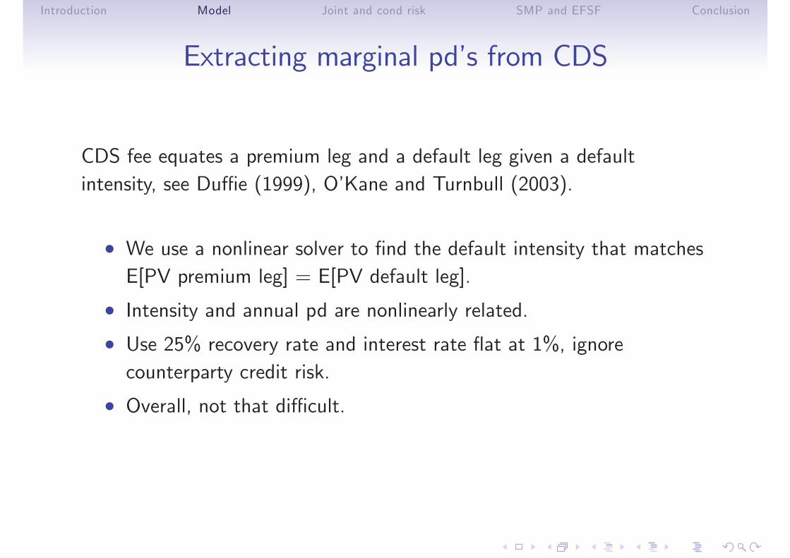
Extracting marginal pd’s from CDS

CDS fee equates a premium leg and a default leg given a default

intensity, see Duffie (1999), O’Kane and Turnbull (2003).

• We use a nonlinear solver to find the default intensity that matchesE[PV premium leg] = E[PV default leg].

• Intensity and annual pd are nonlinearly related.• Use 25% recovery rate and interest rate flat at 1%, ignore

counterparty credit risk.

• Overall, not that difficult.

Introduction Model Joint and cond risk SMP and EFSF Conclusion

Marginal pd’s from CDS

2008 2009 2010 2011 2012 2013

0.025

0.050

0.075

0.100

0.125

0.150

0.175

0.200

AustriaBelgiumGermanySpainFranceGreeceIrelandItalyThe NetherlandsP ortugal

Introduction Model Joint and cond risk SMP and EFSF Conclusion

Pr[ 2 or more credit events ]

Pr[2 or more credit events], one year horizon

2008 2009 2010 2011 2012 2013

0.025

0.050

0.075

0.100

0.125

0.150

0.175

0.200

For comparison: announcement of SMP and EFSF on 10 May 2010

26 July 2012

02 Aug 2012

06 Sep 2012

Pr[2 or more credit events], one year horizon

Introduction Model Joint and cond risk SMP and EFSF Conclusion

Pr[ 2 or more credit events ]

Wessel, D: "ECB’s Tutorial in Successful Jawboning", WSJ, 09 Jan 2013.

Introduction Model Joint and cond risk SMP and EFSF Conclusion

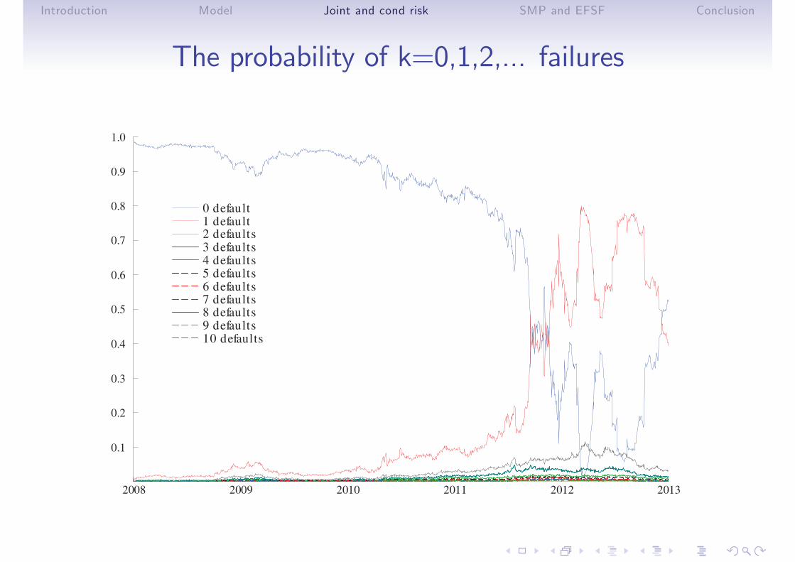
The probability of k=0,1,2,... failures

0 default

1 default

2 defaults

3 defaults

4 defaults

5 defaults

6 defaults

7 defaults

8 defaults

9 defaults

10 defaults

2008 2009 2010 2011 2012 2013

0.1

0.2

0.3

0.4

0.5

0.6

0.7

0.8

0.9

1.0

0 default

1 default

2 defaults

3 defaults

4 defaults

5 defaults

6 defaults

7 defaults

8 defaults

9 defaults

10 defaults

Introduction Model Joint and cond risk SMP and EFSF Conclusion

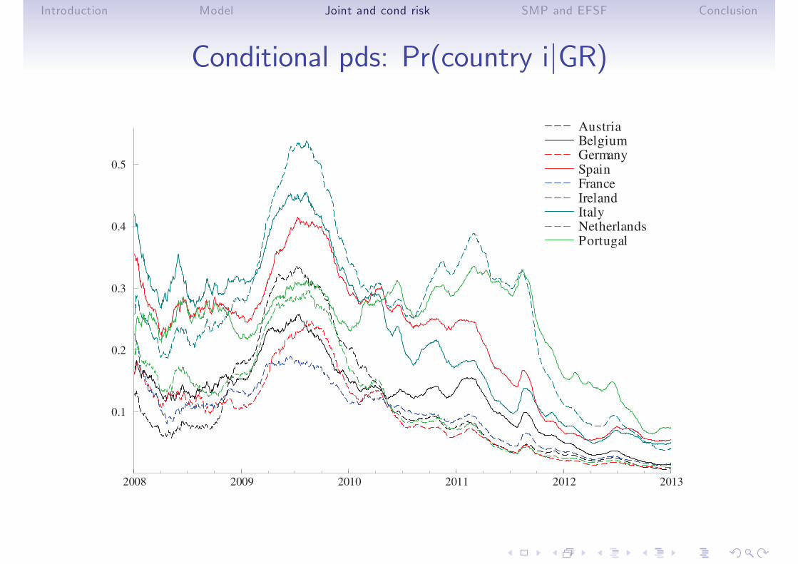
Conditional pds: Pr(country i|GR)

AustriaBelgiumGermanySpainFranceIrelandItalyNetherlandsPortugal

2008 2009 2010 2011 2012 2013

0.1

0.2

0.3

0.4

0.5

AustriaBelgiumGermanySpainFranceIrelandItalyNetherlandsPortugal

Introduction Model Joint and cond risk SMP and EFSF Conclusion

The SMP/EFSF package, 10 May 2010

Joint risk, Pr(i ∩ j)

Thu 06 May 2010 Tue 11 May 2010

PT GR ES PT GR ES

AT 1.1% 1.1% 1.0% 0.6% 0.7% 0.5%

BE 1.2% 1.4% 1.1% 0.9% 1.0% 0.8%

DE 1.0% 1.1% 0.9% 0.8% 0.8% 0.6%

ES 3.0% 3.3% 1.5% 1.6%

FR 1.0% 1.0% 0.8% 0.8% 0.9% 0.7%

GR 4.8% 3.3% 2.3% 1.6%

IR 2.6% 3.1% 2.2% 1.4% 1.8% 1.2%

IT 2.8% 2.9% 2.4% 1.4% 1.5% 1.3%

NL 0.9% 0.9% 0.7% 0.6% 0.7% 0.5%

PT 4.8% 3.0% 2.3% 1.5%

Avg 2.0% 2.2% 1.7% 1.1% 1.2% 0.9%

Introduction Model Joint and cond risk SMP and EFSF Conclusion

The SMP/EFSF package, 10 May 2010

Conditional risk, Pr(i | j)Thu 06 May 2010 Tue 11 May 2010

PT GR ES PT GR ES

AT 17% 8% 26% 22% 10% 27%

BE 20% 10% 28% 32% 15% 40%

DE 16% 8% 23% 26% 12% 30%

ES 49% 25% 50% 23%

FR 16% 8% 22% 28% 12% 35%

GR 78% 87% 80% 81%

IR 43% 23% 57% 49% 26% 58%

IT 45% 22% 63% 49% 21% 65%

NL 14% 7% 19% 21% 10% 24%

PT 36% 79% 33% 74%

Avg 33% 16% 45% 40% 18% 48%

Bottom line: joint risks ↓↓, but dependence ↑ / → .

Introduction Model Joint and cond risk SMP and EFSF Conclusion

The OMT annoucement(s)

Joint risk, Pr(i ∩ j)

Thu 24 Jul 2012 Fri 07 Sep 2012

PT GR ES PT GR ES

AT 1.2% 1.4% 1.2% 0.8% 0.7% 0.7%

BE 1.8% 2.4% 2.0% 1.3% 1.5% 1.5%

DE 0.9% 1.1% 0.9% 0.8% 0.9% 0.9%

ES 3.8% 7.0% 2.5% 4.0%

FR 1.6% 2.1% 1.8% 1.1% 1.3% 1.2%

GR 9.5% 7.0% 5.6% 4.0%

IR 4.3% 6.4% 3.5% 2.7% 4.2% 2.6%

IT 3.5% 6.2% 5.0% 2.5% 3.5% 3.2%

NL 1.2% 1.4% 1.0% 1.0% 1.1% 1.1%

PT 9.5% 3.8% 5.6% 2.5%

Avg 3.1% 4.1% 2.9% 2.0% 2.5% 2.0%

Announcements on 26 Jul 12, 02 Aug 12, and 06 Sep 12.

Introduction Model Joint and cond risk SMP and EFSF Conclusion

The OMT annoucement(s)

Conditional risk, Pr(i | j)Thu 24 Jul 2012 Fri 07 Sep 2012

PT GR ES PT GR ES

AT 11% 1% 16% 11% 1% 15%

BE 17% 3% 26% 20% 2% 31%

DE 8% 1% 11% 11% 1% 19%

ES 35% 8% 37% 5%

FR 15% 2% 23% 17% 2% 25%

GR 87% 90% 83% 83%

IR 40% 7% 45% 40% 5% 54%

IT 32% 7% 64% 37% 4% 66%

NL 11% 2% 13% 15% 1% 22%

PT 10% 48% 7% 52%

Avg 28% 5% 37% 30% 3% 41%

Bottom line: joint risks ↓↓, but dependence ↑ / → . "Firewall"-analogy?

Introduction Model Joint and cond risk SMP and EFSF Conclusion

Conclusion

We proposed a novel modeling framework to infer conditional and

joint probabilities for sovereign default risk from observed CDS.

Based on a dynamic skewed—t multivariate density with time-varying

volatility and correlations.

Central bank lage-scale asset purchase program announcements (such as

SMP, OMT) affected joint risk primarily through impact on marginal

risks, not perceived connectedness.

This project is funded by the European Union

under the 7th Framework Programme

(FP7-SSH/2007-2013) Grant Agreement n°320270

www.syrtoproject.eu