Conditional Frequentist Sequential Tests for the Drift of

Brownian Motion

By Rui Paulo∗

National Institute of Statistical Sciences

and

Statistical and Applied Mathematical Sciences Institute

Abstract

In this paper, we consider the problem of sequentially testing simple hypotheses con-

cerning the drift of a Brownian motion process from a unified Bayesian and frequentist

perspective.

The conditional frequentist approach to testing statistical hypotheses has been utilized

in a variety of settings to produce tests that are virtually equivalent to their objective

Bayesian counterparts. Herein, we show that, at least for standard classes of stopping

boundaries, the unified theory developed so far does not directly apply to the problem

at hand. We thus motivate the need for a new conditioning strategy that ensures the

existence of a conditional frequentist test whose answer essentially matches the objective

Bayesian test. Under a quite general set of assumptions, we show that the new form

of conditioning can still be interpreted as conditioning on the evidence present in the

data as represented by P -values. Further properties of the resulting procedure, including

ancillarity of the partition associated to the conditioning statistic and the characterization

of the no-decision region, are studied in detail in the setting of the familiar sequential

probability ratio test.

∗Research was supported by the U.S. National Science Foundation, Grants DMS-0073952 at the National

Institute of Statistical Sciences, DMS-0103265, and the Statistical and Applied Mathematical Sciences Insti-

tute. This research formed part of the author’s Ph.D. thesis at Duke University, where he was supported by

a Ph.D. Fellowship awarded by Fundacao para a Ciencia e a Tecnologia, Portugal, with reference PRAXIS

XXI/BD/15703/98.

1 Introduction

1.1 Testing the Drift of Brownian Motion

Suppose we are interested in sequentially testing simple hypotheses concerning the

drift parameter, θ, of a Brownian motion process, W (t), t ≥ 0, starting at the

origin. Without loss of generality (see Section 2.1) one can assume that the problem

is of the form

H0 : θ = 0 versus H1 : θ = θ0 , (1.1)

where θ0 > 0. A sequential test of (1.1) is simply a pair (τ, δ), where τ is a stopping

time and δ is the terminal decision rule, which states which decision to take upon

stopping.

An important example of a sequential test for this scenario is the sequential

probability ratio test (SPRT), introduced in its general formulation by Wald (e.g.

Wald, 1947) and studied in detail for the case of Brownian motion by Dvoretzky

et al. (1953). It possesses the attractive pre-experimental property that there is no

other test with at least as low unconditional error probabilities that has a smaller

expected sample size under either hypotheses. It is described as follows: one should

stop observing the process at the stopping time

τ = inft : Bθ0

t 6∈ (a, b) , (1.2)

where 0 < a < 1 < b < ∞ are fixed constants and Bθ0

t , which is defined in (2.1),

can be interpreted as the likelihood ratio of H1 to H0 (cf. Section 2.1). Since the

Brownian motion paths are continuous a.s., upon stopping at τ = t it will either be

Bθ0

t = a or Bθ0

t = b. If the likelihood ratio process exits the set (a, b) at b, one should

reject H0; otherwise, one should reject H1. Let R = IBθ0

τ = b = Ireject H0.

It is easy to show that the test will terminate with probability one under either

hypotheses, i.e., that the stopping rule (1.2) is proper, and furthermore, using the

Optional Sampling Martingale Theorem, it is possible to explicitly compute the

unconditional properties of this test, which we will state here for future reference:

α =

0R = 1 =1 − a

b− a(1.3)

β =

θR = 0 = ab− 1

b− a. (1.4)

1

From an objective Bayesian perspective, the situation is also straightforward.

Since Bθ0

t is a likelihood ratio, it is also the Bayes factor in favor of H1, and as

a consequence, upon stopping at τ = t, the posterior probability of H1 (assuming

each hypothesis is equally likely a priori) is

PH1 | W (s), 0 ≤ s ≤ t, τ = t =Bθ0

t

1 +Bθ0

t

, (1.5)

whereas the posterior probability of H0 is

PH0 | W (s), 0 ≤ s ≤ t, τ = t =1

1 +Bθ0

t

. (1.6)

Note that when H0 is rejected, and therefore Bθ0

τ = b is observed, the reported

frequentist error probability depends on the quantity a. In contrast, the Bayesian

answer depends exclusively on the observed data since Bθ0

τ depends only on the

observed data (and is, indeed, a sufficient statistic). It is, in part, this clash between

the unconditional error probabilities and the objective Bayesian error probabilities

that we seek to alleviate by producing a conditional frequentist test appropriate for

this situation, which essentially agrees with the objective Bayesian test.

Often, the simple versus simple structure is just an approximation to a more

complex situation. For instance in the clinical trials setting, the drift of the process

is related to the added efficacy of a new treatment over a standard. In that case,

the null hypothesis stands for no improvement, while θ0 represents the minimum

improvement that is of practical interest. As such, the interval (0, θ0) is called

the ‘indifference region.’ Unfortunately, precisely in this indifference region, the

expected sample size is in general relatively large. In an effort to address this prob-

lem, Anderson (1960) introduced the triangular boundaries that we will describe in

Section 2.2.

The pre-experimental properties of the ensuing sequential tests are considerably

more involved, and although analytical formulas exist, typically numerical approxi-

mations are needed. As we construct a conditional frequentist test that is applicable

in this situation and furthermore agrees with the Bayesian answer, we will see that

the test is trivial from a computational perspective. The only potential complica-

tion has to do with the so-called no-decision region, but that is seldom of practical

importance (See Section 3.1.)

2

Another point of interest is that the reported error probabilities for the objective

Bayesian test do not depend on the stopping rule used, in accordance with the

Stopping Rule Principle. Since the conditional frequentist test we derive has the

same error probabilities as the Bayesian test, it will also have error probabilities

that abide by that principle.

1.2 Background and Motivation

The Neyman-Pearson approach to testing statistical hypotheses has been criticized

because of its lack of ability to produce data-adaptive measures of conclusiveness

regarding the decisions reached. No matter how extreme the data are — deep into

the rejection region or close to its boundary — one always reports the same (pre-

experimental) error probabilities. Neyman (1942) argues that this is as much as

a theory of testing statistical hypotheses can achieve and still claim a frequentist

interpretation of its conclusions.

Another contentious idea in Statistics is the Stopping Rule Principle, especially

in the area of sequential clinical trials where it has significant ethical implications.

The frequentist approach as long been thought of as incompatible with this principle,

a fact that many people find disturbing and counter-intuitive.

The seminal paper of Berger, Brown and Wolpert (1994), building on work

by Kiefer and co-authors — Kiefer (1976, 1977), Brownie and Kiefer (1977) and

Brown (1978) —, essentially showed that the above conceptions are not true in

general. To be more precise, they showed that, in the simple versus simple case,

it is possible to construct statistical tests that produce sensible data-dependent

measures of conclusiveness and yet have a frequentist interpretation. Furthermore,

these tests essentially abide by the Stopping Rule Principle.

Generalizations of Berger et al. (1994) were carried out in Wolpert (1995), Berger,

Boukai and Wang (1997a,b, 1999), Sellke, Bayarri and Berger (2001), Dass (2001),

Dass and Berger (2003) and Berger (2003). The most relevant reference for the

present article is Berger et al. (1999), where particular emphasis is placed on se-

quential testing. Here, we extend the conditioning strategy described in that paper

to the case of sequential testing of simple hypotheses concerning the drift of a Brow-

nian motion process.

The basic idea behind conditional frequentist testing is very simple, and one of

3

the first attempts at formalizing it dates back to Kiefer (1977): instead of reporting

unconditional type I and type II error probabilities, one should select a suitable

conditioning statistic S, say, measuring ‘strength of evidence in the data,’ and

report error probabilities conditional on the observed value of that statistic, namely

α(s) = Preject H0 | H0, S = s

β(s) = Preject H1 | H1, S = s .

The obvious question is, how should one select in general a suitable S? Berger,

Brown and Wolpert (1994) proposed using Bayesian insight to select S, and indeed

showed that, in simple versus simple problems, one can construct a conditioning

statistic such that the resulting conditional frequentist answer essentially coincides

with the default Bayesian one. More recently, it has been realized that this choice

of S has a particularly interesting interpretation: Sellke et al. (2001) and Berger

(2003) have pointed out that the induced partition matches points on the sample

space that lead to the same P -value when testing H0 versus H1 and vice-versa, in

essence using P -values to measure strength of evidence in the data, as advocated

by Fisher, but converting these P -values into actual error probabilities having a

clear frequentist interpretation, in the spirit of Neyman. The actual answer hap-

pens to numerically coincide with the Bayesian default posterior probability of the

hypotheses, as advocated by Jeffreys.

A by-product of these observations is that, since the final answer coincides with

the Bayesian answer, and Bayesian inference abides by the Stopping Rule Principle,

the resulting procedure necessarily also respects this principle. Indeed, Berger,

Boukai and Wang (1999) showed that, as long as a sequential test satisfies a certain

number of assumptions, this holds even in the simple versus composite problem.

Their paper fully discusses the advantages of this approach, in a sequential setting,

over the standard (unconditional) frequentist approach.

The conditions alluded to above can be summarized as follows. The range of the

likelihood ratio at the stopping time, BN , must be a union of two (not necessarily

disjoint) intervals, and the distribution function of BN must be invertible in its

range under both hypotheses. Also, it is tacitly assumed that the terminal rule is

based on the value of BN alone, and that in particular one can write the rejection

region as BN > r, for a suitable constant r, assuming the likelihood ratio has the

4

likelihood under the null in its denominator. Also, only discrete time is covered.

We will see in Section 2.2 that the standard form of conditioning, developed in

earlier papers, does not apply to the testing problem we address herein, at least

when considering standard stopping boundaries. This clearly motivates the need

for a new conditioning strategy, which we fully describe in Section 2.4.

Interestingly, the new form of conditioning turns out to also possess the P -value

conditioning interpretation that the earlier strategies exhibit, and we explain why

in Section 2.5.

Section 3 explores several aspects of the conditional frequentist test we describe

in this paper. In particular, we address the issue of the presence of the no-decision

region and of the ancillarity (or lack thereof) of the partition associated with the

conditioning strategy we propose.

2 A New Conditioning Strategy and Unified Test

2.1 General Remarks and Notation

Let Ω = C ( +0 ) be the space of all continuous functions ω : +

0 → and F = B(Ω)

the Borel sigma field generated by the sup norm. Consider the coordinate mapping

process Wt(ω) = ω(t) and let W ≡ Wt : 0 ≤ t < ∞. Denote by

θ the measure

defined on (Ω,F ) such that, under

θ, the stochastic process W is Brownian motion

with drift θ with respect to the filtration Ft = σWs, 0 ≤ s ≤ t. In particular,

under

0, W is standard Brownian motion. We will write θ for the expectation

operator under

θ. Note that we have taken the variance parameter σ2 to be

one, which is tantamount to assuming it is a known quantity. This is in fact the

case, since the quadratic variation of the process converges almost surely to σ2,

and therefore observing the process along an interval enables us to calculate an

arbitrarily precise estimate of this parameter.

Recall that we are interested in simple versus simple hypotheses testing problems.

The well-known fact that, if W is Brownian motion with drift θ, then (−W ) is again

Brownian motion but with drift (−θ), and W ? ≡ Wt + ψt, t ≥ 0 is Brownian

motion with drift (θ − ψ) make it evident that one can without loss of generality

assume that the problem is of the form (1.1) with θ0 > 0.

5

Define, for θ 6= 0,

Bθt = exp

(

θWt −12θ2t

)

, t ≥ 0 . (2.1)

Girsanov’s Theorem, cf. Karatzas and Shreve (1991), establishes that for each fixed

T ,

θ(A) = 0[BθT IA] , A ∈ FT (2.2)

where IA stands for the indicator function of the set A. This means that BθT is

the Radon-Nikodym derivative of the restriction to FT of

θ with respect to the

same restriction of

0. Wald’s likelihood ratio identity (cf. Siegmund, 1985) es-

tablishes that furthermore (2.2) is valid if T is replaced by any stopping rule, τ ,

which is proper under both measures

0 and

θ. The quantity (2.1) can therefore

be interpreted as the likelihood ratio of Wt, t ≤ τ under

θ with respect to

0.

2.2 Stopping Boundaries and the Need for a New Condi-

tioning Strategy

Suppose that we observe Brownian motion W (t) starting at the origin and with

drift θ. In order to sequentially test statistical hypotheses concerning the drift pa-

rameter θ, it is common to consider stopping boundaries of the following general

form: two linear boundaries, sometimes complemented with a vertical (or trunca-

tion) boundary at time T . Borrowing from Hall (1997), these can be formalized

asa1 + b1 t for t < T upper

a2 + b2 t for t < T lower

t = T vertical

(2.3)

with a2 < 0 < a1 and 0 < T ≤ ∞; nonetheless, if b2 > b1, it must be T ≤

(a2 − a1)/(b2 − b1), whereas if b2 < b1, then it must be T <∞.

These include as a special case the sequential probability ratio test (SPRT)

boundaries, also referred to as parallel boundaries, when b1 = b2, possibly truncated

(if T < ∞). This type of boundary has been studied in the context of Brownian

motion by Dvoretzky, Kiefer and Wolfowitz (1953). It also includes triangular

boundaries (b2 > b1, with apex at tmax = (a1 − a2)/(b2 − b1), possibly truncated

(T < tmax)), and restricted boundaries (b2 < b1 and T < ∞). These two classes of

6

boundaries were introduced by Anderson (1960) in an effort to reduce the sample

size required by the traditional SPRT.

When testing H0 : θ = 0 versus H1 : θ = θ0, where θ0 > 0, we saw in Section 2.1

that the likelihood ratio is given by expression (2.1). In Figure 1 we have plotted

a few instances of the linear boundaries (2.3) expressed in terms of the likelihood

ratio.

Since the paths of Brownian motion are continuous almost surely, it is clear

that in the case of the open-ended SPRT the likelihood ratio at the stopping time

will assume one of two values. In the truncated version of the SPRT, the range of

the likelihood ratio at the stopping time is indeed an interval, but there is positive

probability that it assumes the upper or the lower limit of that interval, and hence

its distribution function is not invertible in a very important region of the sample

space.

Looking at Figure 1, it is clear that other types of linear boundaries may or may

not satisfy the assumptions of Berger, Boukai and Wang (1999) because, although

the range of the likelihood ratio at the stopping time is indeed an interval, the

terminal decision cannot be expressed exclusively as a function of the statistic Bθ0

t

— in particular, note how it is possible for the same value of Bθ0

t to be on either

the lower or upper boundary, depending on t.

1

PSfrag replacements

Bθ0

t

t

Figure 1: Instances of linear boundaries in the likelihood ratio space.

In effect, we do not know of any commonly used class of stopping boundaries

that, in the context of Brownian motion, always yields a sequential test that satisfies

the needed assumptions, and this clearly motivates the search for a new condition-

ing strategy that assures the matching of the Bayesian and conditional frequentist

7

answers.

2.3 Formal Assumptions

In order to state and prove a general result, we will have to make some assumptions,

especially regarding the stopping rule. To be more specific, we will assume that the

following conditions hold.

Conditions:

(a) The stopping rules we will consider are of the form

τ = inft ≥ 0 : (Bθ0

t , t) 6∈ C (2.4)

where C is the so-called continuation set.

(b) The stopping rule should be proper under both hypotheses:

0τ <∞ =

θ0τ <∞ = 1 . (2.5)

(c) There is a one-to-one and onto correspondence between the observable data

(Bθ0

τ , τ) and the statistic φτ given by

φτ = arctanBθ0

τ − 1

τ. (2.6)

Figure 2 exemplifies the meaning of φτ in the context of the truncated SPRT

test. We will take the branch of the tangent function defined on ] − π/2, π/2[.

(d) The terminal decision rule is such that it can be expressed as

reject H0 iff φτ > c (2.7)

for some constant c.

Since the Brownian motion paths are almost surely continuous, these conditions

are satisfied by all but very strange rules, and they are certainly satisfied by the

class of linear boundaries introduced in Section 2.2.

The last condition that we need deals with the distribution of φτ . We will assume

that the distribution function of φτ is strictly increasing under both hypotheses,

except possibly at a finite number of points. For simplicity, we will denote by Fi(·)

the distribution function of φτ under hypotheses Hi, i.e.

Fi(x) = Pφτ ≤ x | Hi , i = 0, 1 . (2.8)

8

PSfrag replacements

1

Bθ0

t

t

b

φτ

a

Tτ

Figure 2: Schematic representation of the definition of φτ

For completeness, we state

Conditions (cont.):

(e) We assume that for i = 0, 1, Fi(·) is a strictly increasing function, except

possibly at a finite number of points.

Again, this condition will be satisfied virtually always.

2.4 The Conditioning Strategy and Test

We are now in position to describe the conditioning statistic that we will subse-

quently show achieves the unification goal. To that end, define φ? to be the solution

to the equation

1 − F0(φ?) = F1(φ?) , (2.9)

and let

a = c, r = F−11 (1 − F0(c)) if φ? > c

a = F−10 (1 − F1(c)), r = c if φ? < c .

(2.10)

Consider the terminal decision rule

δU =

accept H0 if φτ ≤ a

make no decision if r < φτ < a

reject H0 if φτ ≥ r ,

(2.11)

9

and the conditioning statistic

S = max1 − F0(φτ ), F1(φτ ) . (2.12)

In this setting, we have the following result.

Theorem 2.1 Under Conditions (a)–(e), the conditional frequentist test given by

δU in (2.11) and the conditioning statistic S in (2.12) has conditional error proba-

bilities such that, upon rejection of H0,

α(s) =1

1 +Bθ0

τ

, (2.13)

and, upon acceptance of H0,

β(s) =Bθ0

τ

1 +Bθ0

τ

. (2.14)

Proof: See Appendix A.

Note that this result does not say anything about when to stop, but rather how

to proceed upon stopping. As long as the stopping time belongs to a fairly large

class of rules, then the test just described essentially agrees with its Bayesian default

counterpart and hence it is essentially independent of the stopping rule.

It is clear that certain scenarios covered by the present construction will also

satisfy the assumptions of the strategy described in the Berger et al. (1999) paper.

That will happen whenever τ is of the form

τ = inft ≥ 0 : Bθ0

t ≥ h(t) or Bθ0

t ≤ g(t) (2.15)

where g(t) is increasing, h(t) is decreasing, and g(t) < c < h(t) for some constant c.

If Gi(·) is the distribution function of Bθ0

τ under Hi, i = 0, 1, then the conditioning

statistic introduced in the Berger et al. (1999) paper can be written as

S ′ = max1 −G0(Bθ0

τ ), G1(Bθ0

τ ) . (2.16)

It is easy to check that the partition induced by the statistic S defined by (2.12) and

the one induced by S ′ are indeed the same, so that the present strategy constitutes

in fact an extension of the previous work in the area.

10

2.5 Interpretation as P -value conditioning

As we already mentioned, in the conditional frequentist theory developed so far there

is more to the conditioning statistic than just allowing for the agreement between

the default Bayes and conditional frequentist answers — the statistic actually has a

very important interpretation that allows one to understand how it takes P -values

and converts those quantities into actual errors probabilities. Curiously, the statistic

we have introduced in this paper also shares that attractive feature.

The most important ingredient in defining a P -value is the ordering of the pos-

sible outcomes in terms of the evidence they convey against the null hypothesis. In

a sequential setting that ordering is not always straightforward, and various choices

are in general possible.

In the present setting, the following reasoning is usually accepted as sensible,

cf. Siegmund, 1985, Section III.4. It is clear that

θWt/t > c is an increasing

function of θ for every fixed constant c, so that larger values of Wt/t convey more

evidence against H0. This justifies ordering the observed data in terms of this ratio:

(Wt1 , t1) is perceived as more extreme than (Wt2 , t2) iff Wt1/t1 > Wt2/t2.

At least for the large class of linear boundaries described by (2.3), it is clear that

this argument induces an ordering in the likelihood ratio space such that evidence

increases as one moves along the boundary of the continuation set counterclockwise.

Having seen that, it is now clear that the conditioning statistic S given by (2.12)

matches points in the sample space that lead to the same P -value when testing H0

versus H1 and vice-versa, exactly as in the previously recommended conditioning

strategy.

In the next sections we will study finer details of the proposed conditioning

strategy, such as properties of the no-decision region and the ancillarity of the

associated partition.

3 Properties of the Unified Test

Common concerns regarding the theory of unified testing include the presence of the

no-decision region and the potential lack of ancillarity of the conditioning statistic

S. In this section, we will address these issues in a setting that is particularly

amenable to analytical treatment: that of the open-ended SPRT.

11

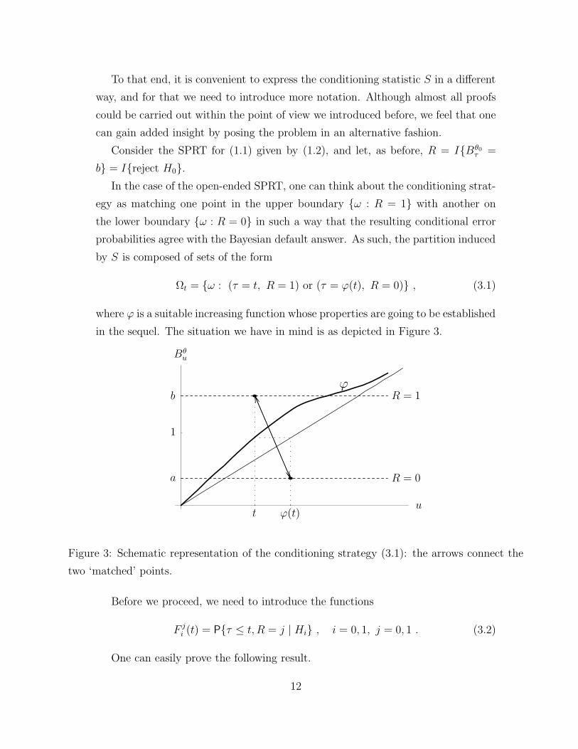
To that end, it is convenient to express the conditioning statistic S in a different

way, and for that we need to introduce more notation. Although almost all proofs

could be carried out within the point of view we introduced before, we feel that one

can gain added insight by posing the problem in an alternative fashion.

Consider the SPRT for (1.1) given by (1.2), and let, as before, R = IBθ0

τ =

b = Ireject H0.

In the case of the open-ended SPRT, one can think about the conditioning strat-

egy as matching one point in the upper boundary ω : R = 1 with another on

the lower boundary ω : R = 0 in such a way that the resulting conditional error

probabilities agree with the Bayesian default answer. As such, the partition induced

by S is composed of sets of the form

Ωt = ω : (τ = t, R = 1) or (τ = ϕ(t), R = 0) , (3.1)

where ϕ is a suitable increasing function whose properties are going to be established

in the sequel. The situation we have in mind is as depicted in Figure 3.PSfrag replacements

1

Bθu

u

bϕ

a

t ϕ(t)

R = 0

R = 1

Figure 3: Schematic representation of the conditioning strategy (3.1): the arrows connect the

two ‘matched’ points.

Before we proceed, we need to introduce the functions

F ji (t) = Pτ ≤ t, R = j | Hi , i = 0, 1, j = 0, 1 . (3.2)

One can easily prove the following result.

12

Proposition 3.1 The function ϕ that corresponds to the partition induced by S

satisfies

F 00 (ϕ(t)) = F 1

1 (t) ⇔ ϕ(t) = [F 00 ]−1[F 1

1 (t)] . (3.3)

Proof: See Appendix B.

In this setting, the no-decision region corresponds to the set of sample points for

which (3.3) has no solution. In the sequel of this section we will study the existence

of solutions to that equation and the related issue of characterizing the no-decision

region.

That study will arm us with results that will allow for a thorough consideration

of the ancillarity of the partition associated with S, and also of the consequences of

the imposition of ancillarity.

3.1 The No-decision Region

There is one circumstance in which ϕ is easy to determine: the case a = 1/b. To

see this, note that, under H1,

1/Bθ0

t ∼

exp−θ0(W?t + θ0 t) + 1

2θ20 t

∼

exp−θ0W?t − 1

2θ20 t

∼

expθ0W?t − 1

2θ20 t

where W ?t is standard Brownian motion and the last step follows from the fact that

if Xt is standard Brownian motion, so is −Xt. We conclude that Bθ0

t | H0 ∼

1/Bθ0

t | H1.

This simple fact enables us to write that, when a = 1/b,

F 00 (t) =

0B

θ0

u hits 1/b before b for some u ≤ t

=

θ01/Bθ0

u hits 1/b before b for some u ≤ t

=

θ0Bθ0

u hits b before 1/b for some u ≤ t

= F 11 (t) ,

and consequently to conclude that ϕ(t) = t. This means that the point (t, b) is

“matched” with the point (t, 1/b). In this case, we have ∪t≥0Ωt = Ω and hence that

the no-decision region is empty.

13

In general, it will not be the case that ∪t≥0Ωt = Ω, meaning that when trying

to match one point of the rejection region with one of the acceptance region, some

of the points will be left unmatched. The situation here is such that the rejection

region is fixed, and therefore if the unconditional test is minimax, i.e. a = 1/b, the

no-decision region is empty; otherwise, one has to introduce the no-decision region,

unless we are willing to reject H0 for some of the points on the lower boundary or

accept H0 for some points of the upper boundary.

The next result characterizes the no-decision region and states the corresponding

probabilities of no decision.

The important fact to retain is that the probabilities of no decision are never

larger than the largest unconditional error probability. Furthermore, the no-decision

region takes place at large t, which, according to the interpretation of the condi-

tioning statistic espoused in Section 2.5, corresponds to the region of the sample

space where the evidences against H0 and against H1, as measured by P -values,

are most similar. This is particularly assuring and reaffirms the idea conveyed by

earlier papers in this subject that the no-decision region is often of no real practical

relevance.

Proposition 3.2 For the open-ended SPRT of (1.1), the no-decision region is of

the form

ΩND =

∅ if a = 1/b

τ > t0, R = 1 if a < 1/b

τ > t1, R = 0 if a > 1/b

(3.4)

where t0 = [F 11 ]−1(1 − α) and t1 = [F 0

0 ]−1(1 − β). The probabilities of no decision,

under the null and under the alternative, satisfy

if a < 1/b,

0 (ΩND) =1

b

1 − ab

b− a≤

θ0

(ΩND) =1 − ab

b− a≤ α (3.5)

if a > 1/b,

θ0(ΩND) = a

ab− 1

b− a≤

0(ΩND) =

ab− 1

b− a≤ β . (3.6)

Above, α and β are respectively given by (1.3) and (1.4).

Proof: See Appendix B.

14

3.2 Ancillarity

In the case of the open-ended SPRT, a statistic equivalent to S in the sense of

inducing the same partition on the sample space, is clearly, in view of (3.1) and

Proposition 3.1, given by

S?(ω) =

ϕ−1(τ) − R × (ϕ−1(τ) − τ) if ω 6∈ ΩND

0 if ω ∈ ΩND .(3.7)

This observation makes it easy to show the following result.

Proposition 3.3 In the case of the open-ended SPRT, the conditioning statistic

S is ancillary if and only if a = 1/b. Moreover, an ancillary partition of the type

described in (3.1) does exist, but leads to conditional error probabilities that match

the unconditional ones given by (1.3) and (1.4).

Proof: See Appendix B.

Proposition 3.3 can indeed be shown to be true in more general settings, but

even in the simple open-ended SPRT context it illustrates a very important point:

the statistic S is in general not ancillary, but the imposition of ancillary can lead

to quite undesirable results. A similar point is illustrated by Example 2 of Berger

et al. (1997a).

4 Acknowledgments

The author would like to thank Professor James Berger for his guidance and insight-

ful discussions. He would like also to thank Professor Robert Wolpert for suggestions

that led to part of the material in this paper.

15

APPENDIX

A Proofs of Section 2

Proof of Theorem 2.1:

According to Wald’s identity ratio, since the stopping time is proper, for any set

A ∈ Fτ ,

θ0(A) = 0B

θ0

τ IA

where IA stands for the indicator function of set A. Hence, we have

θ0φτ ≤ y = 0B

θ0

τ Iφτ ≤ y

=

∫

φτ≤y

Bθ0

τ d

0

=

∫ y

0

Bθ0

τ (u) d

0 φτ ≤ u

where Bθ0

τ (u) corresponds to the value of the likelihood ratio associated to φτ = u

— recall Condition (c). As a consequence, we have that, whenever the derivatives

existddyF1(y) = Bθ0

τ (y) ddyF0(y) . (A.1)

For s 6∈ (a, r), it is possible to show that

Preject H0 | S = s = 1/

1 + 1/ dds

[F0 F−11 ](s)

= 1/

1 +Bθ0

τ [F−11 (s)]

where the last step follows from (A.1). Upon rejection of H0, s = F1(φτ ), which

shows (2.13). The proof of (2.14) is similar and hence omitted.

B Proofs of Section 3

Proof of Proposition 3.1: Looking at Figure 3, let φ be the angle corresponding

to the data (a, ϕ(t)), and φ′ the angle associated to the data (b, t). It is clear that

F 00 (ϕ(t)) =

0φτ ≤ φ = F0(φ) = 1 − F1(φ

′) = F 11 (t) ,

which shows (3.3).

16

Proof of Proposition 3.2: Let us make explicit the dependence of the stopping

rule on the pair (a, b) and F ji (· | a, b). Note that the case a = 1/b has been treated

already, and we showed that F 00 (t | 1/b, b) = F 1

1 (t | 1/b, b).

In the case where a < 1/b, a moment of reflection is enough to convince oneself

that

ω : τa,b ≤ t, R = 0 ⊂ ω : τ1/b,b ≤ t, R = 0

ω : τa,b ≤ t, R = 1 ⊃ ω : τ1/b,b ≤ t, R = 1 ,

which in particular implies that F 00 (t | a, b) ≤ F 0

0 (t | 1/b, b) and F 11 (t | a, b) ≥ F 1

1 (t |

1/b, b). Consequently,

F 00 (t | a, b) ≤ F 0

0 (t | 1/b, b) = F 11 (t | 1/b, b) ≤ F 1

1 (t | a, b)

and we conclude F 00 (t | a, b) ≤ F 1

1 (t | a, b).

Next, we note that limt→+∞ F 11 (t) =

θ0R = 1 = 1 − β > 1 − α. That being

said, it is obvious that the function ϕ is well defined only in the interval [0, t0[,

where t0 = [F 11 ]−1(1 − α). Furthermore, ϕ(t) ≥ t for all t in that interval, and

limt→t0 ϕ(t) = +∞.

Given these properties of ϕ, it is easy to understand that the sample points on

the set ω : τa,b > t0, R = 1 are left ‘unmatched.’ In other words,

Ω =[

∪t∈[0,t0 [Ωt

]

∪ ΩND ,

where ΩND = ω : τa,b > t0, R = 1 is the the region of the sample space where

agreement between conditional frequentists (with this conditioning strategy) and

objective Bayesians does not take place.

It is possible to explicitly calculate the probabilities of no decision, both under

the null and under the alternative:

0(ΩND) =

0R = 1 − F 1

0 (t0 | a, b)

θ0(ΩND) =

θ0R = 1 − F 1

1 (t0 | a, b)

= α−1

bF 1

1 (t0 | a, b) = α− β

=1

b

1 − ab

b− a=

1 − ab

b− a.

We have used the facts that, for all a and b,

F 01 (t) = a F 0

0 (t) (B.1)

F 11 (t) = b F 1

0 (t) . (B.2)

17

which follows easily from the definition and Wald’s likelihood ratio identity.

The case a < 1/b is essentially the reverse situation, and thus is omitted.

Proof of Proposition 3.3: In the case a = 1/b, S? ≡ τ , so that

iS ≤ s =

iτ ≤ s = F 0i (s)+F 1

i (s). This and the fact that F ji = F i

j when a = 1/b (because

of (B.1) and (B.2) and since in that case F 00 (t) = F 1

1 (t)) shows that S? has the same

distribution under both hypotheses, i.e., S?, and hence S, is an ancillary statistic.

The cases a < 1/b and a > 1/b are similar. In both circumstances we have

iS

? ≤ s =

i(ΩND) + F 0i (ϕ(s)) + F 1

i (s) , (B.3)

so that

0S

? ≤ s =

0(ΩND) + (1 + 1/b) F 11 (s)

θ0S? ≤ s =

θ0

(ΩND) + (1 + a) F 11 (s) .

One important distinction between the two situations is that the above formulas

are valid for s ∈ [0, t0[ in the case a < 1/b and for s ∈ +0 when a > 1/b.

When a < 1/b, we can rewrite the last pair of equations as

0S

? ≤ s =1

b

θ0

(ΩND) + (1 + 1/b) F 11 (s)

θ0S? ≤ s =

θ0

(ΩND) + (1 + a) F 11 (s) ,

whereas in the case a > 1/b we have

0S

? ≤ s =

0(ΩND) + (1 + 1/b) F 11 (s)

θ0S? ≤ s = a

0 (ΩND) + (1 + a) F 1

1 (s) .

As a consequence, S?, and hence S, is ancillary if and only if a = 1/b, which proves

the first part of the result.

It is easy to check that a partition of the form of (3.1) with ϕ substituted by ψ

given by the formula

ψ(t) = [F 00 ]−1

[

b− 1

b (1 − a)F 1

1 (t)

]

is ancillary, and that the associated conditional error probabilities coincide with the

unconditional ones.

18

References

Anderson, T. W. (1960). A modification of the sequential probability ratio test

to reduce the sample size. Annals of Mathematical Statistics 31 165–197.

Berger, J. O. (2003). Could Fisher, Jeffreys and Neyman have agreed on testing?

Statistical Science 18 1–32.

Berger, J. O., Boukai, B. and Wang, Y. (1997a). Properties of unified

bayesian-frequentist tests. In Advances in Statistical Decision Theory and Ap-

plications (S. Panchapakesan and N. Balakrishnan, eds.). Birkhauser, Boston,

207–223.

Berger, J. O., Boukai, B. and Wang, Y. (1997b). Unified frequentist and

Bayesian testing of a precise hypothesis (Disc: p149-160). Statistical Science 12

133–148.

Berger, J. O., Boukai, B. and Wang, Y. (1999). Simultaneous Bayesian-

frequentist sequential testing of nested hypotheses. Biometrika 86 79–92.

Berger, J. O., Brown, L. D. and Wolpert, R. L. (1994). A unified conditional

frequentist and Bayesian test for fixed and sequential simple hypothesis testing.

The Annals of Statistics 22 1787–1807.

Brown, L. D. (1978). A contribution to Kiefer’s theory of conditional confidence

procedures. The Annals of Statistics 6 59–71.

Brownie, C. and Kiefer, J. (1977). The ideas of conditional confidence in the

simplest setting. Communications in Statistics, Part A – Theory and Methods 6

691–752.

Dass, S. (2001). Unified Bayesian and conditional frequentist testing for discrete

distributions. Sankya Series B, Indian Journal of Statistics 63 251–269.

Dass, S. and Berger, J. O. (2003). Unified conditional frequentist and Bayesian

testing of composite hypotheses. Scandinavian Journal of Statistics 30 193–210.

19

Dvoretzky, A., Kiefer, J. and Wolfowitz, J. (1953). Sequential decision

problems for processes with continuous time parameter. Testing hypotheses. An-

nals of Mathematical Statistics 24 254–264.

Hall, W. J. (1997). The distribution of Brownian motion on linear stopping

boundaries. Sequential Analysis 16 345–352.

Karatzas, I. and Shreve, S. (1991). Brownian Motion and Stochastic Calculus.

2nd ed. No. 113 in Graduate Texts in Mathematics, Springer-Verlag, New York.

Kiefer, J. (1976). Admissibility of conditional confidence procedures. The Annals

of Statistics 4 836–865.

Kiefer, J. (1977). Conditional confidence statements and confidence estimators

(C/R: p808-827). Journal of the American Statistical Association 72 789–807.

Neyman, J. (1942). Basic ideas and some recent results of the theory of testing

statistical hypotheses. Journal of the Royal Statistical Society 105 292–327.

Sellke, T., Bayarri, M. and Berger, J. (2001). Calibration of p values for

testing precise null hypotheses. The American Statistician 55 62–71.

Siegmund, D. (1985). Sequential Analysis: Tests and Confidence Intervals.

Springer-Verlag.

Wald, A. (1947). Sequential Analysis. John Wiley and Sons.

Wolpert, R. L. (1995). Testing simple hypotheses. In Studies in Classification,

Data Analysis, and Knowledge Organizaion (H. H. Bock and W. Polasek, eds.),

vol. 7. Springer-Verlag, Heidelberg, 289–297.

National Institute of Statistical Sciences

Statistical and Applied Mathematical Sciences Institute

19 T.W. Alexander Drive

P.O. Box 14006

Research Triangle Park, NC 27709–4006

USA

E-Mail: rui@niss.org

20