
Condition Monitoring - Qucosa: Startseite€¦ · Condition Monitoring...
92
Condition Monitoring Using Computational intelligence methods Master Thesis for the fulfillment of the academic degree M.Sc in Automotive Software Engineering Faculty of Computer Science Professorship of Computer Engineering June 2015 Submitted by: Anwesh Kotta Matr Nr.:300669 Supervisors: Prof. Dr. Wolfram Hardt (TU Chemnitz) Dr.Ariane Heller (TU Chemnitz) Dipl.-Ing. Abdelhakim Laghmouchi (Fraunhofer IPK)
-
Upload
phungduong -
Category
Documents
-
view
218 -
download
0
Transcript of Condition Monitoring - Qucosa: Startseite€¦ · Condition Monitoring...

Condition MonitoringUsing Computational intelligence methods
Master Thesis
forthe fulfillment of the academic degree
M.Sc in Automotive Software Engineering
Faculty of Computer ScienceProfessorship of Computer Engineering
June 2015
Submitted by: Anwesh KottaMatr Nr.:300669
Supervisors: Prof. Dr. Wolfram Hardt (TU Chemnitz)Dr.Ariane Heller (TU Chemnitz)Dipl.-Ing. Abdelhakim Laghmouchi (Fraunhofer IPK)

Acknowledgement
This master thesis would not be possible without the extensive support and encourage-ment of many people. I am very grateful to my mentors Prof. Dr. Wolfram Hardt andDr. Ariane Heller who supported me throughout my master’s degree. It is only with theguidance of Prof. Dr. Hardt, I have been able to successfully pursue by master thesisat Fraunhofer IPK, Berlin under the department of Production Machines and SystemsManagement.
I would like to acknowledge and extend my heartfelt gratitude to my master thesisadvisor, Mr. Abdelhakim Laghmouchi, for his constant guidance and support duringmy thesis work. I am very thankful to Daniel Reißner for supervising my work at theuniversity. I wish to acknowledge Fraunhofer IPK for giving me an opportunity to pursuemy master thesis and technical support provided to me during my thesis work.
I would like to thank all the members of the Production Machines and System Manage-ment for their warm welcome and the great working environment they created.
Finally, I would like to thank my family, without their continuous support this workwould not have been possible.
Thank you.
i

Abstract
Machine tool components are widely used in many industrial applications. Inaccordance with their usage, a reliable health monitoring system is necessary todetect defects in these components in order monitor machinery performance and
avoid malfunction. Even though several techniques have been reported for fault detectionand diagnosis, it is a challenging task to implement a condition monitoring system in realworld applications due to their complexity in structure and noisy operating environment.The primary objective of this thesis is to develop novel intelligent algorithms for a reliablefault diagnosis of machine tool components. Another objective is to use Micro ElectroMechanical System (MEMS) sensor and interface it with Raspberry pi hardware for thereal time condition monitoring.
Primarily knowledge based approach with morphological operators and Fuzzy InferenceSystem is proposed, the effectiveness of this approach lies in the selection of structuringelements(SEs). When this is evaluated with different classes of bearing fault signals, itis able to detect the fault frequencies effectively. Secondarily, An analytical approachwith multi class support machine is proposed, this method has uniqueness of learning onits own with out any prior knowledge, the effectiveness of this method lies on selectedfeatures and used kernel for converging. Results have shown that RBF (Radial BiasFunction) kernel, which is commonly known as gauss kernel has good performance inidentifying faults with less computation time. An idea of prototyping these methods hastriggered in using Micro Electro Mechanical System (MEMS) sensor for data acquisitionand real time Condition Monitoring. LIS3DH accelerometer sensor is used for the dataacquisition of spindle for capturing high frequency fault signals. The measured data isanalyzed and compared with the industrial sensor k-shear accelerometer type 8792A.
ii

Table of Contents
Page
List of Figures vi
List of Tables viii
1 Introduction 11.1 Overview . . . . . . . . . . . . . . . . . . . . . . . . . . . . . . . . . . . . 11.2 Thesis Organization . . . . . . . . . . . . . . . . . . . . . . . . . . . . . . 2
2 State of the Art 32.1 Related works . . . . . . . . . . . . . . . . . . . . . . . . . . . . . . . . . 32.2 Stages in Condition Monitoring (CM) . . . . . . . . . . . . . . . . . . . . 6
2.2.1 General Approach of Condition Monitoring . . . . . . . . . . . . . 72.3 Basics related to this work . . . . . . . . . . . . . . . . . . . . . . . . . . 11
2.3.1 Fault detection and diagnosis . . . . . . . . . . . . . . . . . . . . 112.3.2 Vibration Monitoring System (VMS) . . . . . . . . . . . . . . . . 112.3.3 Data used in Condition Monitoring (CM) . . . . . . . . . . . . . 132.3.4 Morphological Analysis (MA) . . . . . . . . . . . . . . . . . . . . 15
2.4 Summary . . . . . . . . . . . . . . . . . . . . . . . . . . . . . . . . . . . 15
3 Support Vector Machine (SVM) in Condition Monitoring 173.1 Introduction . . . . . . . . . . . . . . . . . . . . . . . . . . . . . . . . . . 173.2 Theory of Support Vector Machine . . . . . . . . . . . . . . . . . . . . . 19
3.2.1 Multi class Support Vector Machine . . . . . . . . . . . . . . . . . 233.3 Developed Concept for Roller Bearing Fault Diagnosis using Support
Vector Machine . . . . . . . . . . . . . . . . . . . . . . . . . . . . . . . . 283.3.1 Data Acquisition . . . . . . . . . . . . . . . . . . . . . . . . . . . 283.3.2 Feature Extraction . . . . . . . . . . . . . . . . . . . . . . . . . . 29
iii

TABLE OF CONTENTS
3.3.3 Feature Selection . . . . . . . . . . . . . . . . . . . . . . . . . . . 303.3.4 Multi class Support Vector Machine Classification . . . . . . . . . 31
3.4 Summary . . . . . . . . . . . . . . . . . . . . . . . . . . . . . . . . . . . 31
4 Fuzzy Set Theory in Conditon Monitoriong 324.1 Introduction . . . . . . . . . . . . . . . . . . . . . . . . . . . . . . . . . . 324.2 Computational Intelligence . . . . . . . . . . . . . . . . . . . . . . . . . . 334.3 Developed Concept for Fault Diagnosis using Morphological Analysis and
Fuzzy Inference System (MAFIS) . . . . . . . . . . . . . . . . . . . . . . 404.4 Summary . . . . . . . . . . . . . . . . . . . . . . . . . . . . . . . . . . . 41
5 Implementation and Integration 435.1 Development Environment . . . . . . . . . . . . . . . . . . . . . . . . . . 435.2 Experimental Data . . . . . . . . . . . . . . . . . . . . . . . . . . . . . . 445.3 Fraunhofer IPK’s Condition Monitoring Tool . . . . . . . . . . . . . . . . 45
5.3.1 Structure of the Tool . . . . . . . . . . . . . . . . . . . . . . . . . 465.4 Implementation of Muti class Support Vector Machine . . . . . . . . . . 51
5.4.1 Performance Evaluation . . . . . . . . . . . . . . . . . . . . . . . 555.5 Impimentation of Morphological Analysis and Fuzzy Inference System . . 56
5.5.1 Morphological Analysis (MA) . . . . . . . . . . . . . . . . . . . . 585.5.2 Fuzzy Inference System (FIS) . . . . . . . . . . . . . . . . . . . . 61
5.6 Summary . . . . . . . . . . . . . . . . . . . . . . . . . . . . . . . . . . . 63
6 Embedded Implementation 646.1 Development Board . . . . . . . . . . . . . . . . . . . . . . . . . . . . . . 646.2 MEMS Vibration Sensor . . . . . . . . . . . . . . . . . . . . . . . . . . . 656.3 Preparing Raspberry . . . . . . . . . . . . . . . . . . . . . . . . . . . . . 66
6.3.1 Sensor Interface . . . . . . . . . . . . . . . . . . . . . . . . . . . . 666.3.2 I2C Communication . . . . . . . . . . . . . . . . . . . . . . . . . 676.3.3 SPI Communication . . . . . . . . . . . . . . . . . . . . . . . . . 69
6.4 Sensor Position and Measurement . . . . . . . . . . . . . . . . . . . . . . 706.5 Suppor Vector Machine Implementation on Raspberry Pi . . . . . . . . . 72
6.5.1 Development Environment . . . . . . . . . . . . . . . . . . . . . . 726.6 Evaluation of Spindle Data . . . . . . . . . . . . . . . . . . . . . . . . . . 73
6.6.1 Computation time on Raspberry . . . . . . . . . . . . . . . . . . 776.7 Summary . . . . . . . . . . . . . . . . . . . . . . . . . . . . . . . . . . . 78
iv

TABLE OF CONTENTS
7 Conclusion and Future Work 79
Bibliography 81
v

List of Figures
Figure Page
2.1 Reliability curve for machinery failure [2] . . . . . . . . . . . . . . . . . . . . 42.2 Failures occur in a machinery [2] . . . . . . . . . . . . . . . . . . . . . . . . 42.3 Failures in a rotating machinery [3] . . . . . . . . . . . . . . . . . . . . . . . 52.4 Costs associated with maintenance strategies [2] . . . . . . . . . . . . . . . 62.5 Condition Monitoring System (CMS) stages [4] . . . . . . . . . . . . . . . . 72.6 Condition Monitoring System (CMS) components[4] . . . . . . . . . . . . . . 82.7 Failures symptops of components over time [2] . . . . . . . . . . . . . . . . . 92.8 Steps involved in VBCMS[2] . . . . . . . . . . . . . . . . . . . . . . . . . . . 122.9 Signal view in time and frequency domain [9] . . . . . . . . . . . . . . . . . 14
3.1 Libsvm for linear classification [14] . . . . . . . . . . . . . . . . . . . . . . . 213.2 Concept of MSVM for faut Diagnosis . . . . . . . . . . . . . . . . . . . . . . 293.3 Overview of time domain feature extraction [3] . . . . . . . . . . . . . . . . . 30
4.1 MF curve defining transition not tall to tall . . . . . . . . . . . . . . . . . . 344.2 Straight line MF’s defined over specific range [17] . . . . . . . . . . . . . . . 354.3 Curved MF’s with specific range[18] . . . . . . . . . . . . . . . . . . . . . . 354.4 Interpretation of If then rules . . . . . . . . . . . . . . . . . . . . . . . . . . 374.5 Concept of MAFIS for Fault diagnosis . . . . . . . . . . . . . . . . . . . . . 404.6 Membership funtions range [12] . . . . . . . . . . . . . . . . . . . . . . . . . 41
5.1 Test rig for roller bearing data acquisition [19] . . . . . . . . . . . . . . . . . 445.2 Condition monitoring toolbox (Fraunhofer IPK) [19] . . . . . . . . . . . . . 465.3 Data structure of the toolbox . . . . . . . . . . . . . . . . . . . . . . . . . . 475.5 (a)Time Domain IR small fault (b)Frequency Domain IR small fault 485.6 (a)Time Domain IR small fault (b)Frequency Domain IR small fault 495.7 (a)Time Domain OR small fault (b)Frequency Domain OR small fault 49
vi

List of Figures
5.8 (a)Time Domain OR heavy fault (b)Frequency Domain OR heavyfault . . . . . . . . . . . . . . . . . . . . . . . . . . . . . . . . . . . . . . . . 49
5.9 Feature Extraction . . . . . . . . . . . . . . . . . . . . . . . . . . . . . . . . 505.10 Classification window . . . . . . . . . . . . . . . . . . . . . . . . . . . . . . . 515.11 Preparing data set for classification . . . . . . . . . . . . . . . . . . . . . . . 535.12 Performance analysis of all methods . . . . . . . . . . . . . . . . . . . . . . . 595.13 Fuzzy rules for fault classification . . . . . . . . . . . . . . . . . . . . . . . . 625.14 Detected frequency peak of IR fault . . . . . . . . . . . . . . . . . . . . . . . 625.15 Detected frequency peak of OR fault . . . . . . . . . . . . . . . . . . . . . . 63
6.1 Raspberry pi configuration menu . . . . . . . . . . . . . . . . . . . . . . . . 676.2 Sensor connected with Raspberry . . . . . . . . . . . . . . . . . . . . . . . . 696.3 Sensor mounted next to spindle ball screw . . . . . . . . . . . . . . . . . . . 706.4 Measured data- Sensor Position far from spindle . . . . . . . . . . . . . . . . 716.5 Measured data- Sensor Position closer to spindle . . . . . . . . . . . . . . . . 716.6 Signal split for different speeds . . . . . . . . . . . . . . . . . . . . . . . . . 726.7 Folder structure on Raspberry . . . . . . . . . . . . . . . . . . . . . . . . . . 736.8 3D feature space of faults at 1000 mm/min speed . . . . . . . . . . . . . . . 746.9 3D feature space of faults at 2000 mm/min speed . . . . . . . . . . . . . . . 746.10 3D feature space of faults at 3000 mm/min speed . . . . . . . . . . . . . . . 756.11 3D feature space of faults at 4000 mm/min speed . . . . . . . . . . . . . . . 756.12 3D feature space of faults at 5000 mm/min speed . . . . . . . . . . . . . . . 76
vii
List of Tables
Table Page
5.1 No of data files used for evaluation . . . . . . . . . . . . . . . . . . . . . . . 455.2 Amount of data used for training and testing . . . . . . . . . . . . . . . . . 465.3 Classification accuracy of MSVM . . . . . . . . . . . . . . . . . . . . . . . . 555.4 Computational time for all methods . . . . . . . . . . . . . . . . . . . . . . . 59
6.1 Market analysis on different development boards . . . . . . . . . . . . . . . . 646.2 Cost comparison between proposed approach and conventional approach . . 656.3 Market analysis for different MEMS sensors . . . . . . . . . . . . . . . . . . 666.4 SPI pin connectivity between raspberry and LIS3DH . . . . . . . . . . . . . 686.5 SPI pin connectivity between raspberry and LIS3DH . . . . . . . . . . . . . 696.6 Package required for Python on raspberry . . . . . . . . . . . . . . . . . . . 736.7 Classification accuracy at different speeds . . . . . . . . . . . . . . . . . . . 776.8 Computation speed comparison between pc and raspberry pi for 6 features . 786.9 Computation speed comparison between pc and raspberry pi for 3 features . 78
viii

Ch
ap
te
r 1Introduction
Condition monitoring is defined as the continuous or periodic measurement andinterpretation of data to indicate the condition of an item and also to determinethe need for maintenance [1].
1.1 Overview
Industrial machineries are composed of various subsystems, such as electrical drivesystems, controlling units and actuators, these components are involved in performing thedesired operation of machines. The availability and efficient utilization of these machineriesare the key factors in effecting the economy of manufacturing company. When thereis any deadlock during the operation of machineries due to scheduled or unscheduledmaintenance, component or process failure will have a negative effect on both availabilityand utilization. Structural components of a machinery such as bearings, spindles andball screws are subjected to wear over the time. Monitoring of these components on aregular basis is therefore necessary to reduce the risk of failures and breakdowns. Forinstance, these breakdown of these components can lead to unexpected failure in themachinery and they should be detected in early stages.
Condition monitoring of wear susceptible machinery have been a challenging task forthe researchers and engineers mainly in industries. The primary objective of this thesis isto research and implement different condition monitoring algorithms using computationalintelligence methods for the wear susceptible machinery. The proposed methods use the
1
CHAPTER 1. INTRODUCTION
vibration data that has been acquired from roller bearing test rig for the evaluationof different fault signals, to scale the performance of these algorithms. Although thereare many methods in performing the Condition Monitoring, early fault diagnosis canbe achieved through vibration analysis and diagnosis. This work mainly focuses ondeveloping efficient algorithm for Vibration Based Condition Monitoring (VBCM) andalso to develop a system which is cost effective in VBCM. Although there are manymethods in performing the Condition Monitoring, early fault diagnosis can be achievedthrough vibration analysis and diagnosis. This work mainly focuses on developing efficientalgorithm for VBCM and also to develop a system which is cost effective in VBCM.
Another objective is to develop hardware for data acquisition of ball screw usingMEMS sensor and also to deploy these methods into the hardware for reliable and costeffective Condition Monitoring.
Condition monitoring definition: "The process of systematic data collection andevaluation to identify changes in performance or condition of a system, or its components, so that remedial action may be planned in a cost effective manner to maintain reliability"[23].
1.2 Thesis Organization
The first chapter gives a glance about Condition Monitoring and current trends in theindustry in regard with different measurement factors. The second chapter deals withcurrent industry problems and basic building blocks and fundamentals that are necessaryin employing a Condition Monitoring system. The third and fourth chapter addressesthe core side of Condition Monitoring System (CMS), where different computationalintelligence methods used in CMS are discussed. Third and fourth chapters present thetheory behind two different approaches namely knowledge based approach and analyticalapproach, that used in the Condition Monitoring of machine tool components. The fifthchapter highlights the implementation part, which throws light on both the approaches.The sixth chapter is an idea to deploy these methods into an embedded hardware, it alsodiscusses the results of cost effective MEMS sensors used for real time data acquisitionand condition monitoring.
2
Ch
ap
te
r 2State of the Art
2.1 Related works
Continuous health monitoring and establishing stable working of machining processesin a machinery is of major importance to reduce the risk of malfunctioning equipment,ensuring high quality of parts that are produced by the machinery. This can be possibleby testing of the critical machine tool components and online measuring and analysis oneor more parameters of the machining process in order to attain stable working process.The curve shown in Fig.2.1 shows the unexpected failure rate Vs time in a machinery [2],where β < 1 represents decrease in failure rate, β = 1 represents constant failure rate,and β > 1 represents an increase failure rate over time [2].
Fig.2.2 shows total failure components in side a wind turbine and survey was done on1500 wind turbines and for a duration of 15 years. For the successful diagnosis of thesefailures is to find and analyze all the occurring causes, which lead to component failure andensuring condition based maintenance to these components. This approach of conditionbased maintenance mainly helps in machine diagnosis when making modifications on thecomponent that has no fault .
The major causes in component failure of the rotating machinery can be varied.These causes can be due to high ambient temperature, persistent overloading, abnormalmoisture, abnormal voltage and frequency, high vibration, aggressive chemicals, poorlubrication, poor ventilation or cooling, normal age deterioration. Simple probabilisticapproaches are used to estimate the reliability levels of these machinery. Research shows
3

CHAPTER 2. STATE OF THE ART
Figure 2.1: Reliability curve for machinery failure [2]
Figure 2.2: Failures occur in a machinery [2]
that there are three major components of faults in a rotating machinery : stator faults,bearing faults and rotor faults as shown in Fig.2.3.
4

CHAPTER 2. STATE OF THE ART
Figure 2.3: Failures in a rotating machinery [3]
. Costs associated with the maintenance strategies is shown in Fig. By observing thecurves, preventive strategy will reduce the failures but will be expensive. In reactivemaintenance strategy number of faults and cost for the repair are high but low cost inprevention.
Thus we need intelligent maintenance, a combination of preventive and reactive toimprove reliability, availability and maintainability of machine tool components. Thiscan be achieved by performing condition monitoring on these components.
5

CHAPTER 2. STATE OF THE ART
Figure 2.4: Costs associated with maintenance strategies [2]
2.2 Stages in Condition Monitoring (CM)
The main objective of any CM process is to predict the state of health of a machine ora structure from the measure data [4]. This can be carried out in five stages, which isshown in Fig.2.5.
First stage is detection of presence or absence of fault. feature identification and pulseshape analysis of measured data are most commonly used methods for fault detection.
Second stage is fault classification which is commonly refereed as fault diagnosis,at this stage we not only detect the detect the fault but also find the nature of fault(e.g.,which category the fault falls in). Differnt computational methods are used inclassifying the types of faults.
Third stage is identification of fault location.Fourth stage is quantification of fault. It gives the magnitude fault, i.e, how severe
the faultFifth stage is estimating the remaining useful life of the machine component or
structure being monitored.
6

CHAPTER 2. STATE OF THE ART
Figure 2.5: Condition Monitoring System (CMS) stages [4]
2.2.1 General Approach of Condition Monitoring
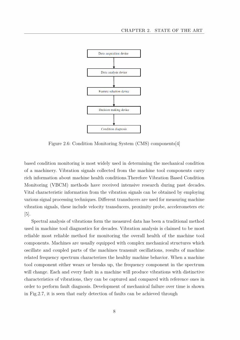
In building a CMS there are different stages involved. each and every stage is itselfhas individual components or subsystem , all these these constitute together to formcondition monitoring system [4]. The fig.2.6 below gives a glance idea for building anyCMS
In accordance with the sensor measurements used, The most common conditionmonitoring techniques which are currently used in the machinery are:
• Vibration analysis
• Oil/debris condition analysis
• Temperature monitoring
• Acoustic emission monitoring
• Current/power monitoring
2.2.1.1 Vibration Analysis
There are so many approaches developed for the condition monitoring of machinery.Even though there are many approaches used in condition monitoring, the vibration
7
CHAPTER 2. STATE OF THE ART
Figure 2.6: Condition Monitoring System (CMS) components[4]
based condition monitoring is most widely used in determining the mechanical conditionof a machinery. Vibration signals collected from the machine tool components carryrich information about machine health conditions.Therefore Vibration Based ConditionMonitoring (VBCM) methods have received intensive research during past decades.Vital characteristic information from the vibration signals can be obtained by employingvarious signal processing techniques. Different transducers are used for measuring machinevibration signals, these include velocity transducers, proximity probe, accelerometers etc[5].
Spectral analysis of vibrations form the measured data has been a traditional methodused in machine tool diagnostics for decades. Vibration analysis is claimed to be mostreliable most reliable method for monitoring the overall health of the machine toolcomponents. Machines are usually equipped with complex mechanical structures whichoscillate and coupled parts of the machines transmit oscillations, results of machinerelated frequency spectrum characterizes the healthy machine behavior. When a machinetool component either wears or breaks up, the frequency component in the spectrumwill change. Each and every fault in a machine will produce vibrations with distinctivecharacteristics of vibrations, they can be captured and compared with reference ones inorder to perform fault diagnosis. Development of mechanical failure over time is shownin Fig.2.7, it is seen that early detection of faults can be achieved through
8

CHAPTER 2. STATE OF THE ART
Figure 2.7: Failures symptops of components over time [2]
Most of the faults generated in the mechanical components cause vibrations withdifferent characteristic frequencies. The percentage of vibration diagnosis in the industrieshas increased over the years, since it is found that mechanical vibrations are more accurateand precise indicators of a machine condition. The vibration analysis can be used todetect stress in the form of imbalance, alignment errors, fitting problems, and electricaldefects etc., therefore condition monitoring and fault detection systems mostly employvibration based techniques. However major disadvantages of vibration monitoring arehigh cost and sensors and equipment are inevitably subject to failure. As a result thiscauses additional problems with system reliability and maintenance costs.
2.2.1.2 Oil/Debris Analysis
Lubricants are widely used in almost all moving parts of machinery in order to reducethe friction, wear and tear and also for the purpose of cooling. Damages in engines occurwhen there are any chemical reactions or contamination due to the foreign particles fromthe environment of the machine. These changes can deteriorate the lubricating functionand cooling mechanism over the time which further causes the wear and tear of themachine. Sensors will continuously measure the viscosity, temperature, specific electricalconductivity and also the dielectric constant of the medium. Changes in these parametersgive the information about the aging process of the lubricant [6]. Sensors use opticalnear-infrared reflectance method to verify the quality of grease during the operation ofroller bearings. The lubricant oil monitoring can optimize the time for the exchange ofthe lubricant and also to predict the possible defects in the machine based on the oil
9

CHAPTER 2. STATE OF THE ART
state [5].
2.2.1.3 Temperature monitoring
Temperature should be in a certain range during the operation conditions of machinery[7]. Temperature is the most common indicator in regard with the structural health ofmachinery equipment and components. Damages around corroded electrical connections,material components, etc., can cause abnormal temperature distribution [5]. As tem-perature is most useful parameter that indicates the structural health of components,monitoring the temperature of machinery can be undoubtedly one of the best way ofpredictive maintenance method. Major disadvantage of temperature monitoring is thattemperature change is determined by various factors. For example bearing tempera-ture depends on bearing fault, generator rotating speed, environment temperature..etc.therefore it is complicated to only relay on temperature monitoring of machine toolcomponents.
2.2.1.4 Acoustic emission monitoring
Acoustic emission monitoring provides significant improvement (from 1 kHz to 2 MHz)over vibration monitoring, when there is a situation with high surrounding noise [8]. AEbased method provides the real-time measurement of friction and mechanical shocks ofoperating machinery. By measuring the shock and friction events, AE technique is ableto detect wear and damage at the earliest stages and this also enables the tracking ofdefect progression throughout the failure process. This is possible because as the damageprogresses, the energy measured for any friction and shock events increases. The obtainedstress energy graph is then used as a reference to the measured and tracked againstnormal machine operating conditions.
The digital analysis of stress signal involves in computing both the amplitude andenergy of the detected stress signals. The amplitude peak of the signal is a function of theintensity of single friction or a shock event. The disadvantage of AE emission monitoringis high cost, since the frequency range of AE signal is up to 100 MHz, the sensors usedand data acquisition equipment are expensive than other fault detection methods.
2.2.1.5 Current/power monitoring
Wear of electrically controlled units will often lead to higher power consumption. Thismeans that there is an important need for the measurement of energy consumption and
10
CHAPTER 2. STATE OF THE ART
its maintenance. By the means of current-voltage relationship the power consumption ofelectric motors, coils, and transformers can be monitored [5]. For example deterioration bywear will lead to unusual fluctuations in the performance and efficiency. Major advantageof current/power monitoring is it uses the current and/or measurements of the controlsystem of the machine; no additional sensors or data acquisition is required. However thereare some challenges in using current, voltage signals for the condition monitoring andfault detection. The useful information from the current, voltage signals has nonstationarystatistics due to the variable speed of machine. It is difficult to extract fault signaturesfrom nonstationary signals by using traditional spectrum analysis methods.
2.3 Basics related to this work
2.3.1 Fault detection and diagnosis
• Fault detection: Identification of failure in a machinery with out knowing theroot cause.
• Fault diagnosis: Finding root causes for the failures, to the point where correctiveactions can be taken.
2.3.2 Vibration Monitoring System (VMS)
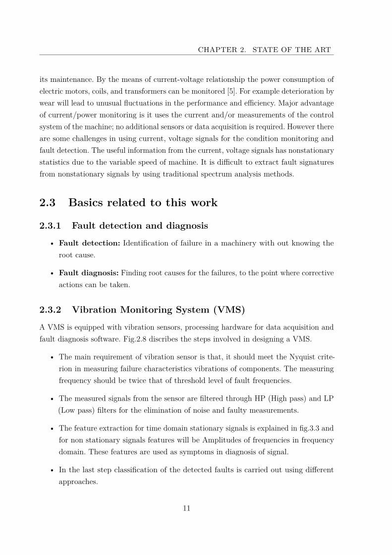
A VMS is equipped with vibration sensors, processing hardware for data acquisition andfault diagnosis software. Fig.2.8 discribes the steps involved in designing a VMS.
• The main requirement of vibration sensor is that, it should meet the Nyquist crite-rion in measuring failure characteristics vibrations of components. The measuringfrequency should be twice that of threshold level of fault frequencies.
• The measured signals from the sensor are filtered through HP (High pass) and LP(Low pass) filters for the elimination of noise and faulty measurements.
• The feature extraction for time domain stationary signals is explained in fig.3.3 andfor non stationary signals features will be Amplitudes of frequencies in frequencydomain. These features are used as symptoms in diagnosis of signal.
• In the last step classification of the detected faults is carried out using differentapproaches.
11
Figure 2.8: Steps involved in VBCMS[2]
CHAPTER 2. STATE OF THE ART
2.3.3 Data used in Condition Monitoring (CM)
There are four major domains in the representation of data: Time domain, frequencydomain, time frequency domain, modal domain. The raw data is measured in time domain[4]. Fourier transformation can be used to transform the measured data into frequencydomain. The modal properties of the signal can be extracted from frequency domain,sometimes directly from time domain.
2.3.3.1 Time Domain
Time domain data is measured data over a period of time, which is unprocessed. someform of statistical features such as mean,variance are extracted when time domain dataare used. For example a higher displacement output can convey the shifting of the anydevice beyond its limit or a increase in temperature can convey greater friction thanexpected. Deducing something from signals based on its changes over time domain datais known as Time Domain Analysis.
2.3.3.2 Modal Domain
Modal domain data are segmented as natural frequencies, mode shapes and dampingratios.
• Natural frequencies: By analyzing the shifts that occur in natural frequencies, whichare caused by change in condition of structures or machines the structural faultscan be identified. But these changes are small in magnitudes and this limits thatthe level of fault that natural frequencies can identify to high magnitudes.
• Damping ratios: Damping ratios are used to detect the presence of fault in structures,this has been applied to composite materials. –studied the changes of compositematerials, observed that delamination of graphite increased the damping ration ofspecimen.
• Mode shapes: Mode shapes are properties of a structure, which show physical topol-ogy of structure at various natural frequencies. However, they are computationallyexpensive to identify, susceptible to noise due to modal analysis. These are easyto implement for fault detection and mostly in detecting large faults which aredirectly linked to shape of the structure.
13

CHAPTER 2. STATE OF THE ART
2.3.3.3 Frequency Domain Analysis (FDA)
Frequency Domain Analysis is done when the measured time domain signal isconverted into a equivalent frequency domain signal (F = 1/T ) and then signalcomponent frequencies are analyzed.Jean Baptiste Fourier is the one who formulatedmathematical equations for visualizing the frequency spectrum of a time basedsignal [9]. Time-frequency transformation can be shown in fig.2.9
Figure 2.9: Signal view in time and frequency domain [9]
Energy from the generated pulse signal is distributed over a range of frequenciesby transforming the acquired signal into frequency domain, individual frequencycomponents with their corresponding amplitudes can be obtained. In real timeanalysis, the result of transformation should be fast. Frequency domain analysiscomes under real time analysis which makes the use of Fast Fourier Transformation(FFT) algorithm for the calculation of spectrum to the blocks of data. This is anefficient way of discrete fourier transformation. The equations below describe thebasic relationships of signal transformation from time domain signal to frequencydomain signal and vice versa [10].
(2.1) Sx(f)=∞∫−∞
x(t)e−i2πftdt
(2.2) x(t)=∫ ∞−∞
Sx(f)e−i2πftdf
14

CHAPTER 2. STATE OF THE ART
where
x(t) is time history
Sx(f) is fourier transformation of x
DFT pair equivalent to equation (2.1) and (2.2)
(2.3) Sx(m∆f)=∆tn−1∑i=0
x(n∆t)e−i2∏m∇fn∆t
2.3.4 Morphological Analysis (MA)
Morphological signal processing involves in decomposing the original signal into severalphysical parts according to certain geometric characteristics. This method is free fromthe drawbacks of other signal processing methods like FFT, which cannot be used fornonlinear and non-stationary signals and when it comes to wavelet transform method, ithas the problem of mode fixing for empirical mode decomposition (EMD) and also it needsa long time to compute basic wavelet [11]. The main advantage of morphological filter isit requires less computational time than other signal processing methods Morphologicalanalysis is a nonlinear spatial analysis method, mostly used in image processing. Thebasic idea in morphological analysis to transform the shape of the signal through theintersection another object called structuring element (SE). SE is determinative factorfor morphological operations, it has decisive effect on the analysis . The effectiveness ofthe morphological analysis relies on the structuring element chosen. Feature extractionand de-noising can be achieved by constantly moving SE to match the signal. Flat SEs(height =1) are considered more in most of the cases because they are simple and shapeof the SE has little effect on the analysis. The only parameter to be considered is thelength of SE, which is very crucial. Santhana and Murali [12] have a new method forselecting the better SE based on the kurtosis value. The idea is to dispose ten SEs ofdifferent lengths upon considering the range of the fault frequency threshold and selectthe SE which has maximum kurtosis value for the analysis.
2.4 Summary
• Different components failures that occur in machinery are discussed with thepossible causes of failure.
• Need for the condition based maintenance is illustrated form the fig.[2.4].
15

CHAPTER 2. STATE OF THE ART
• Stages of condition monitoring involves, finding the remaining useful life of compo-nents for the pleasant operation of the machinery to avoid future failures.
• Different data domains are explained, how the signal in frequency domain will showthe spectrum of important frequencies in frequency domain.
• why the vibration monitoring is a very effective way in determining structuralfailures of comments is discussed. A simple construction of vibration monitoringsystem is explained from the components to diagnosis.
• How the morphological analysis is more efficient in extracting vibrational impulsesfrom signals is discussed using structuring element.
16

Ch
ap
te
r 3Support Vector Machine (SVM) in Condition
Monitoring
This chapter summarizes and review recent research and developments of SVM inCondition Monitoring.
3.1 Introduction
In recent times, the development of conditioned based maintenance strategy is supportedby computer technology both in hardware and software. The recent advancements madeuse of artificial intelligence (AI) techniques as tool for condition based maintenance. Theidea of reliable, effective and easy maintenance has lead the practical maintenance to thelevel of Intelligent maintenance system . Intelligent maintenance system consists of partslike hardware and software, which are used for the system to perform maintenance routinelike human being. The use of expert system (ES) as a branch of AI in maintenanceis one solution. The basic idea of ES is simply that expertise, which is the transferof task-specific knowledge from a human to a computer. This knowledge is stored inthe computer and users call upon the computer for specific assistance as needed. Thecomputer can make inferences and arrive at a specific conclusion with out any humanhelp. And also, like human consultant, it gives advice and explains the logic behind theadvice.
Support vector machine is a computational learning method which is based on super-
17

CHAPTER 3. SUPPORT VECTOR MACHINE (SVM) IN CONDITIONMONITORING
vised learning theory, it can serve as ES. SVM roots are based on Vapnik Chervonenkis(VC) theory which is a general mathematical framework in learning dependencies offinite data samples. VC theory combines fundamental concepts and self-consistent math-ematical theory, well-defined formulation and principles related to learning. Moreover,concepts of VC-theory can be used for improved understanding various machine learningmethods developed in statistics, fuzzy systems, signal processing and neural networksetc [13]. A major conceptual contribution of VC-theory is revisiting the problem state-ment appropriate for modern supervised learning method that makes a clear distinctionbetween the problem formulation and solution approach. Considering VC dimension,the bounds on the generalization are optimized using a training algorithm, proposed inthat automatically maximizes the margin between the training patterns and the decisionboundary. There are Numerous algorithms for the classification of faults for machinetool diagnostics such as Bayesian classifier, Discriminant analysis, SVM and ArtificialNeural Networks.SVM belong to the family of kernel methods, this method is highlypopular in the field of supervised machine learning. It has several benefits when comparedwith other statistical classifiers like MLPs. MLP and RBF networks don’t care aboutthe quality of classification i.e, they stop converging in finding the hyper plane thatcorrectly classifies the training data. Hyper plane is the classifier which separates twodistinct classes. If the number of hidden neurons in NN is big, the training error becomessmall and this increases the generalization error, computational complexity and thismakes the usage intractable. The most significant benefit of SVM is higher efficiency inhigh dimensional nonlinear classification problems while the other statistical classifiersoften fail in achieving it. The idea is to maximise the margin between hyper plane andthe training examples. This can be done by finding the optimal hyper plane which hasmaximal margin.
The problem of nonlinear classification can be solved by mapping the original datainto higher dimensional feature space which has to be done in accordance with coverstheorem on the separability of patterns (1965). The computations is implicitly done bymeans of kernel function, by defining dot product between points in the feature space.This is called kernel trick while the linear algorithm only relies on the inner productbetween input vectors.
SVM been used successfully in many real-world classification problems like text catego-rization, image classification, Bioinformatics (Protein classification, Cancer classification),and hand-written character recognition [14]. Here we use SVM to learn the characteristicsof vibration signals for different fault classes in the measured data and to predict class of
18

CHAPTER 3. SUPPORT VECTOR MACHINE (SVM) IN CONDITIONMONITORING
the unknown measured signal. Training of the SVM is done offline and best SVM modelfor classification is selected based on cross validation. New data can be given to selectedmodel either offline measured data or online later.
In the condition monitoring and fault diagnosis problem, SVM is employed forrecognizing special patterns from acquired signal, and then these patterns are classifiedaccording to the fault occurrence in the machine [15]. After signal acquisition, a featurerepresentation method can be performed to define the features, e.g., statistical featureof signal for classification purposes. These features can be considered as patterns thatshould be recognized using SVM
3.2 Theory of Support Vector Machine
Classical learning methods are usually designed to minimize the generalization errorwhen training the data set and this called as empirical risk minimization (ERM). Neuralnetworks are best example for methods which follow ERM. In contrast, SVM follow theapproach of structural risk minimization (SRM), a derived approach from statisticallearning theory . SVM is designed in achieving better minimization generalization error[16].
SVM is more efficient in handling very large datasets, the dimensions of classifiedvectors does not effect the performance of SVM. On the other hand dataset dimensionshas distinct influence on conventional classifiers that is why SVM is considered to be moreefficient in dealing with large classification problems. This will give advantage in choosingmore statistical features in the case of fault diagnosis. In training the SVM Classifierthe minimization structural miss classification error is being done, whereas conventionalclassifiers are trained in such a way to reduce emphirical risk. SVM performance insolving various classification problems can be e.g., in Christiani and Shawe-Taylor [14].
Considering the input data to be xi(i=1,2, ..,M), where m is the number of samples.The samples of this data set xi assumed to have two classes namely positive and negativeclasses. Each of classes are associated with class labels be yi=1 for positive class and yi=−1for negative class, respectively. Considering this linear data classification problem, thehyperplane (which determines the class boundary) f(x)=0 that separates the considereddata set is given by
(3.1) f(x)=wTx b=M∑j=1
wjxj b=0
19

CHAPTER 3. SUPPORT VECTOR MACHINE (SVM) IN CONDITIONMONITORING
where ’w’ is M -dimensional vector and b represents a scalar. The position of hy-perplane separating the classes is adjusted in accordance with the vector w and scalarb. The decision function for determining the newly given input variable is made usingsign(f(x)), which creates separating hyperplane that classify data in either positive classor negative class. This hyperplane constructed should satisfy the following constraintsfor linear classification
f(xi)=1 if yi=1
f(xi) =−1 if yi=−1(3.2)
or this can be presented in complete equation
(3.3) yif(xi)=yi(wTx b)≥ 1 for i=1,2, ...,M
SVM algorithm converges in finding the hyperplane which has maximum distance betweenthe data points, it is called optimal hyperplane. An example of the optimal hyperplaneof separating two data sets is presented in fig.3.1
Fig.3.1 shows a series data points with two different classes of data, wherein whitecircles represent positive class and black squares represent negative class. The SVMclassifier tries to make a linear class boundary between these two different classes, andorientate this hyperplane in such way that the margin for the data points is maximized,which is represented with dotted line. SVM classifier also attempts to adjust the hyper-plane to ensure that the distance between the hyperplane and the nearest data point ofeach class is maximal (creates maximum functional margin). Therefore, the boundary isplaced in the middle of this margin between two points, The nearest data points whichdefine the define the margin are called support vectors, the grey circles and squares aredata points which constitute to support vectors. Support vectors are the data in both theclasses which have unit functional margin. Functional margin of ith example in datasetis defined as the distance of point from hyperplane. when the data points which are usedto define the support vectors are determined the rest of the feature set is not need, thesesupport vectors contains all the information needed for defining the classifier. From thegeometry the geometrical margin is found to be ||w||−2
Slack variables are the data points which are on and other side the margin i.e,between support vectors and hyperplane. The optimal hyperplane can be obtained whenconsidering slack variables ξi and the error penalty C by in solving the optimizationproblem,:
20

CHAPTER 3. SUPPORT VECTOR MACHINE (SVM) IN CONDITIONMONITORING
Figure 3.1: Libsvm for linear classification [14]
(3.4) minimize 12 ||w||
2 CM∑j=1
ξi
(3.5) subject to {yi(wTx b)≥ 1− ξi, i=1, . . . ,M,
ξi ≥ 0, i=1, . . . ,M
where ξ is the measuring distance between margin and the data points xi lying on thewrong side i.e, slack variables. This optimization problem can be simplified by
(3.6) minimize L(w,b,α)=12 ||w||
2−M∑i=1
αiyi(w.xi b)M∑i=1
αi.
T w and b, while the derivatives of L to α need to vanish. At the optimal point, we havethe following saddle-point equations:
(3.7) ∂L
∂w=0 ∂L
∂b=0
which replacing into form
(3.8) w=M∑i=1
αiyixi,M∑i=1
αiyi=0
21

CHAPTER 3. SUPPORT VECTOR MACHINE (SVM) IN CONDITIONMONITORING
From Eq. (3.8), we find that w is vector containing subspace of dataset xi. Bysubstituting Eq. (8) into Eq. (6), we obtain dual quadratic optimization problem [? ]maximize
(3.9) L(α)=M∑i1αi−
12
M∑i,j=1
αiαjyiyjxixj
(3.10) which subject to αi ≥ 0, i=1, . . .M,M∑i=1
αiyi
Thus, by solving this dual optimization problem, we obtain the coefficients αi, which isrequired to express the w to solve Eq. (3.4). This leads to non-linear decision function.
(3.11) f(x)=signM∑i,j=1
αiyi(xixj) b
Non linear classification problems can also be solved using SVM, with the use ofkernel functions . The non linear data can be mapped into high dimensional featurespace, where the data can be linearly separable. The use of non linear function φ(x) =(φ(x), . . . ,φl(x)) to map the n-dimensional input space vector x onto l dimensionalfeature space, the decision function for this dual form is given by
(3.12) f(x)=sign (M∑i,j=1
αiyi(φT (xi).φ(xj) b)
In other words giving flexibility to eliminate slack variables, this constructed hy-perplane is said to be Soft margin classifier. SVM is nothing but soft margin classifierequipped with Kernel function. Working on high-dimensional features space no onlyenables the expression of complex decision functions, but it also generates computationalproblem. Over fitting problem arises due to high dimensionality problem and also thisleads to computational problem due to large vectors. Kernel functions solve these prob-lems by reducing the number of computations. Kernel function returns the dot productof feature space of data set mapped, given as K(xi,xj) = (φT (xi).φ(xj)). When kernelfunction is applied the learning in feature space don’t need φ evaluation explicitly andthe decision function will be:
(3.13) f(x)=sign (M∑i,j=1
αiyiK(xi,xj) b).
22

CHAPTER 3. SUPPORT VECTOR MACHINE (SVM) IN CONDITIONMONITORING
This method is called "kernel trick", kernel functions have been introduced for differenttypes of sequence data,text,graphs,images, as well as vectors. The efficiency of the SVMdepends on the selected kernel. Generally gauss Radial Bias Function (RBF) kernelis preferred for most of the applications. Most widely used kernel functions and theirrepresentations are listed below
Kernel Functions Representationkernel K(x,xj)Linear xT .xj
Polynomial (γxTxj r)d,γ ≥ 0Gaussian RBF exp(−‖x−xj‖2/2γ2)
Any function which satisfies mercer’s theorem can be used as a kernel function tocompute a dot product in feature space for the reduction of dimensionality. The selectionof the appropriate kernel function is very important, since the kernel mapping givesthe feature space to which training data points needs to be classified. The definition oflegitimate kernel function is given in mercer’s theorem, the function must be continuousand positive definite. I
3.2.1 Multi class Support Vector Machine
The above discussion deals with binary classification, where the class labels can takeonly two values: 1 and -1. In the real-world classification problems, however, we findmore than two classes for examples: the fault diagnosis of rotating machineries like rollerbearing there are several fault classes such as Inner ring damage, outer ring damage, balldamage, cage damage etc. Therefore, in this section the multi-class classification strategyusing SVM will be discussed[14].
3.2.1.1 One Vs All (OVA)
One Vs All is the earliest implemented for multi class problems [14]. It builds k numberof SVM models, where k is the number of different classes, where the ith SVM modelis trained with all of examples in the ith class of dataset with positive labels, and restof examples from all other classes with negative labels. For given l training dataset(x1,y1), . . . ,(xl,yl), Where xi ∈Rn,1=1, . . . , l and yi ∈ 1, . . . ,k is the class of xi, the ithSVM can solve the following problem: minimize:
(3.14) 12‖w
i‖2 Cl∑
i=1ξij(wi)T
23

CHAPTER 3. SUPPORT VECTOR MACHINE (SVM) IN CONDITIONMONITORING
subject to:
(3.15) (wi)Tφ(xj) bi ≥ 1− ξij if y=i,
(3.16) (wi)Tφ(xj) bi ≤−1 ξij if y 6 i,
(3.17) ξij ≥ 0, j=1, . . . , l,
where the training data with model xi is mapped to a higher-dimensional space byfunction φ and C, as the penalty parameter.
Minimizing Eq. (3.14) means we would like to maximize 2/‖wi‖, the margin between
two groups of data. When dataset is not linearly separable the penalty parameter Cl∑
i=1ξij ,
will reduce the number of training errors.The Fig shows OVA classification for three different classes by constructing three
different hyperplanes, where each hyperplane is used to classify one class with rest of allclasses
24


CHAPTER 3. SUPPORT VECTOR MACHINE (SVM) IN CONDITIONMONITORING
3.2.1.2 One Vs One (OVO)
Another major method is known as One Vs One method. This approach builds k(k−1)/2hyperplanes where each class is trained on data from two classes [14]. In training datasetfrom the ith and the jth classes, it can be solved as binary classification problem.
minimize:
(3.18) 12‖w
ij‖2 C∑t
ξijt (wij)T
subject to:
(3.19) (wij)Tφ(xt) bij ≥ 1− ξijt if yt=i,
(3.20) (wij)Tφ(xt) bij ≤−1 ξijt if yt=j,
(3.21) ξijt =0, j=1, . . . , l,
Different methods are used to test k(k−1)/2 classifiers that are constructed. Aftertest, the decision in choosing the model is done using this strategy: sign ((wij)Tφ(xt) bij)tells x is in ith class, then the vote for the ith class is raised by one. Otherwise, the jthvote is raised by one. x is predicted for the class which has highest votes. The votingmethod described is called as Max Win strategy.
26


CHAPTER 3. SUPPORT VECTOR MACHINE (SVM) IN CONDITIONMONITORING
3.3 Developed Concept for Roller Bearing FaultDiagnosis using Support Vector Machine
In this section, the review of condition monitoring and fault diagnosis using SVM will beaddressed to machines, which have symptoms lead to failure.
Here we give an overview about SVM classification and how this method is transformedin order to classify multiple classes. Then we explain the concept behind the constructionof hyper sphere which is analogous to hyper plane in linear classification. The work flowfor this concept is shown in the block diagram below:
3.3.1 Data Acquisition
Roller bearings has widespread of domestic and industrial application, which include allbearings which make use of rolling action in machinery in order to reduce the friction. Inindustrial Machinery, these components are considered as critical components and defectsin these bearings, not detected in time causes malfunctioning and may even lead to theunexpected failure of whole machinery. Early detection of faults is important from systemview point of maintenance and process automation. The typical occurrence of failure iscaused when there is fault or scratch on the surface of the bearing, which is results surfacefatigue of the bearing due the repeated loading of rotating shaft and it is difficult to avoidthis in operating conditions. Whenever a defective surface makes contacts with matchingsurface placed it will generate a short pulse and this will resonate whole bearing assembly.If the bearings are rotating at constant speed then these pulses will be generated with aperiodic frequency, this frequency is a function of bearing geometry, rotational rate andfault location. There is lot of research on bearing fault detection and fault diagnosis.
In this concept test case of roller bearing, machine casing acceleration is measurean used for fault detection. This can be done by mounting piezoelectric accelerometerexternally over the machine casing, preferably near or on the roller bearing housing. Sincemost of the machinery faults are due to temperature increase, piezoelectric sensors are notmore sensitive to temperature this allows the bearing vibration to transmit through thestructure of transducer. Main reason for considering accelerometer is that they have theadvantage of providing a wide dynamic frequency range of measurement. Accelerometersare found to be more reliable and accurate of the vibration transducers available.
28

CHAPTER 3. SUPPORT VECTOR MACHINE (SVM) IN CONDITIONMONITORING
Figure 3.2: Concept of MSVM for faut Diagnosis
3.3.2 Feature Extraction
Feature extraction constitutes in construction of feature matrix and selection of featuresfrom the data, i.e, feature construction and feature selection. Feature selection is necessaryto select relevant features, a good feature extraction can achieve:
• Data reduction, to limit storage requirements and increase algorithm speed;
• Feature matrix reduction, to save resources in the next round of data collection orduring utilization;
• Performance improvement, improves prediction accuracy;
• Data understanding, visualization of data on a feature space for better knowledgeand understanding of data
In general the vibration data measured contains series of velocity, proximity, accelera-tion values. The time domain features that can be computed for this data are shown inFig[2.8]
Fig.3.3 shows the statistical features used in time domain to construct feature matrix.If the number of features are too high, it will increase the dimensionality and this in turn
29

CHAPTER 3. SUPPORT VECTOR MACHINE (SVM) IN CONDITIONMONITORING
Figure 3.3: Overview of time domain feature extraction [3]
increases the number of computations. If the features are less then it will directly effectthe performance of algorithm. Feature extraction can be done by extracting the timedomain signal characteristics like mean, variance, kurtosis etc. from the raw accelerationdata. Feature vector has to be constructed upon these calculated statistical parameters.Different fault classes will have unique statistical parameters, SVM model is trainedbased on these parameters.
• Mean
• RMS value
• Kurtosis
• Variance
• Skewness
3.3.3 Feature Selection
Feature selection is crucial for the development of classification model. Proper featureselection can help to simplify the design of SVM model. On the other hand, improperfeature selection will deteriorate the performance of SVM. Here we have used sequentialfeature selection method for finding the goodness of selected features which are useful indesigning a model. Research suggests that changing the sensor data will directly reflecton selected features i.e. different sensor measurements are will have different featureswhich are good in classification.
30

CHAPTER 3. SUPPORT VECTOR MACHINE (SVM) IN CONDITIONMONITORING
3.3.4 Multi class Support Vector Machine Classification
Although SVM’s have good efficiency in various classification applications, one of theirdrawbacks is that they are confined to 2 class classifiers. In many real world applicationslike fault classification of machine tools, it should be able to classify multi class classifi-cation problem. This problem can be solved by decomposing multi class into several 2class problems, training these linear classifiers and reconstructing the solution from theoutput of individual classifiers. The simplest way is to do one vs. others classificationand combining these classifiers output. In this method N classifiers are built in way thateach classifier separates one class from rest of all, Where N is number of unique classes.
3.4 Summary
This chapter outlines different multi class classification approaches of SVM and how thegeneralized SVM works in building a hyper plane in solving a classification problem.Thereare several algorithms for the classification of faults for machine tool diagnostics suchas Bayesian classifier, Discriminant analysis, SVM and Artificial Neural Networks.SVMbelong to the family of kernel methods, this method is highly popular in the field ofsupervised machine learning. It has several benefits when compared with other statis-tical classifiers like MLPs. MLP and RBF networks do not care about the quality ofclassification i.e, they stop converging in finding the hyper plane that correctly classifiesthe training data. Hyper plane is the classifier which separates two distinct classes. Ifthe number of hidden neurons in NN is big, the training error becomes small and thisincreases the generalization error, computational complexity and this makes the usageintractable.
The most significant benefit of SVM is higher efficiency in high dimensional nonlinearclassification problems while the other statistical classifiers often fail in achieving it. Theidea is to maximize the margin between hyper plane and the training examples. Thiscan be done by finding the optimal hyper plane which has maximal margin. Reason forchoosing the MSVM with One vs ALL approach is that, it needs less computationalpower and convergence speed is better than other approach One Vs One classification.
31

Ch
ap
te
r 4Fuzzy Set Theory in Conditon Monitoriong
4.1 Introduction
Over the years, Fuzzy theory has been applied successfully in many number of applications.Some of these include relating operators in chemical plants on their skill availability,age and health, in pattern recognition and in control systems. The main advantage ofFuzzy Set Theory (FST) is the capability to model the uncertainty of many systemsand environments exhibit. This enables FST to explore the interaction of variables thatdefine a system, and how each of these variables affect the system’s behavior.
This chapter unveils the FST for the Condition Monitoring of wear susceptiblemechanical components. In essence, this chapter presents the application of FST todiagnose the condition of roller bearings. This procedure applies Morphological analysis(MA) for the data from the roller bearing test bench. Faults produced in rotatingmachinery can be traced as impulses in the vibration signal, they are represented byunique frequency peaks. These signals are modulated with a number of high frequencycomponents resulting from the structural response to individual impacts. This results inloss of characteristic frequency in the noise, however morphological operators can be usedfor removing noise and to extract the characteristic peaks of a vibration signal. Whenfuzzy rules are trained based on the morphological analysis of different fault signals, thetrained fuzzy system can now be used for the detection of faults for unknown signals. InMA there is a relationship between the resulting failure and impulses extracted usingmorphological operation. The beauty of this approach is MA combined with FST makes
32
CHAPTER 4. FUZZY SET THEORY IN CONDITON MONITORIONG
the condition monitoring on line for the early detection of faults. Implementing FST onroller bearing data is essential because the degree at which the assessment standard isunder the cut off or threshold point for a safe operation of bearings. This inconsistencyto be accounted for the assessment procedure by applying FST. Impulses extracted arevital measure in the evaluation process and denotes both the operating frequencies ofthe bearings and peaks of fault frequencies that occur during operation.
4.2 Computational Intelligence
This section explains the use of tools namely Fuzzy Logic Theory (FLT), Fuzzy RulesMembership Functions, Decisions based on Fuzzy Rules and Defuzzification [4].
4.2.0.1 Fuzzy Logic Theory
The method Fuzzy Logic is of mapping input space to output space by means of somelisted linguistic rules, which entail to if-then statements. In fuzzy logic we define humanreadable rules to form the target system. For example, considering room temperaturecontrol problem, firstly the uncertainty of the system should be modeled into simple itthen rules:
• If the room is hot then cool it down
• If the room is normal then don’t change temperature
• If the room is cold then heat it up
Basic fuzzy logic comprises four components namely Membership functions, Fuzzysets, Fuzzy logic operators and Fuzzy rules, which map input and output space of asystem.
The aim of the fuzzy logic is to allow more flexible representation of sets of objects bymaking fuzzy sets. A fuzzy set does not have perfect margins like classical set, rather theobjects are characterized by degree of membership to specific set. Accordingly, transitionalvalues of objects can be characterized in a way nearer to that the human brain thinks, ascompared to clear cut-off margins in classical sets.
4.2.0.2 Membership Functions
A membership function specifies the degree of the object characterized into certain setor class. The membership function curve maps the input space variables into numbers
33

CHAPTER 4. FUZZY SET THEORY IN CONDITON MONITORIONG
between 0 to 1, which signifies the degree of confidence weather a specific input variableis the element of specific class or a set. The membership curve can be of any shape.Consider an example of two subsets where one denotes tall people and the other denotesshort ones. In determining a class of an unknown person, partial participation in each ofthese sets is possible. Membership function consequently determines the degree to whicha person is tall or short.
The fig.4.1 shows smoothly varying curve from short to tall. Here the output-axis is anumber known to be membership value between 0 and 1.
Figure 4.1: MF curve defining transition not tall to tall
The condition of a membership function must satisfy is that it must vary between 0and 1. The MF can be itself an arbitrary curve whose shape can be defined as a functionthat improvises from the point of simplicity, speed, convenience and efficiency.
There are wide variety of membership functions, among them simplest membershipfunctions are defined using straight lines. A simple triangular membership function is acollection of three points forming a triangle. A trapezoidal membership function has aflat top with a truncated triangle curve. These straight line membership functions havethe advantage of simplicity as shown in fig.4.2
34

CHAPTER 4. FUZZY SET THEORY IN CONDITON MONITORIONG
Figure 4.2: Straight line MF’s defined over specific range [17]
There are other membership functions which are built on gaussian and polynomialbased curves.The gaussian membership function can be specified with two parameterswhereas bell MF has one more parameter, hence it can approach a non-fuzzy set whenthe free parameter is tuned. Due to their smoothness and concise notation, Gaussianand bell membership functions are popular methods in specifying fuzzy sets. Both ofthese MF curves have the advantage of being smooth and nonzero at all the points.
Figure 4.3: Curved MF’s with specific range[18]
The Three characteristics namely input membership function, If-then rules, andoutput membership function define the characteristics of the fuzzy inference system (FIS)and determine the efficiency to classify the newly given input variables. Therefore, it isimportant to correctly define them.
35

CHAPTER 4. FUZZY SET THEORY IN CONDITON MONITORIONG
Thus in the context of vibration analysis the input and output membership functionsare chosen as simple triangular and the ranges are defined based on the input frequencyrange and provide a way to classify the fault signal.
4.2.0.3 If-then Rules
Fuzzy sets and fuzzy operators constitute to subjects and verbs of fuzzy logic. In orderextract something useful one need to make complete sentences. One such way is conditionalstatements, if-then rules, They make fuzzy logic useful [4]. A simple fuzzy if-then ruleassumes the form
if x is A then y is BHere A and B are linguistic values which are defined by fuzzy sets on the ranges X
and Y, respectively. The if-part of rule "x is A" is called the premise or antecedent, whilethe then-part of rule "y is B" is called the conclusion or consequent. Here is an examplefor such a rule.
if service is good then tip is ok
The antecedent is an interpretation that returns a single number between 0 and 1,whereas consequent is a kind of assignment which assigns the entire fuzzy set B to theoutput variable y. So the word "is" is used in two entirely different ways depending onwhether it comes in the antecedent or the consequent. In terms of programming, this isthe distinction between a relational test using "==" and a variable assignment using the"=" symbol. A less confusing representation of rule would be [18]:
if service == good then tip = okHence the input to an if-then rule is current value for the input variable (service) and
the output belongs to an entire fuzzy set (ok). Interpreting an if-then rule involves twodistinct parts: firstly, evaluating the antecedent (which involves in Fuzzification of inputand applying any necessary fuzzy operators) and secondly, applying this result to theconsequent (this is known as implication). In the case of binary logic or two valued logic,It is not difficult to define If-then rules. If the antecedent is true, then the consequentis true. When the restrictions of binary or two valued logic is not considered, if theantecedent is true to some degree of membership function cure, then the consequent isalso true to that same degree of membership curve. It can be shown below
In Binary logic: p → q (p and q are either true or false)In fuzzy logic: 0.5 p → 0.5 q (partial antecedents imply partially)
36

CHAPTER 4. FUZZY SET THEORY IN CONDITON MONITORIONG
The antecedent and consequent of a rule may have multiple parts, as given in belowexamples:
multiple antecedent parts:if sky is gray and wind is strong and barometer is falling, then ...In this case all parts are calculated simultaneously and resolved into one single number
on membership curve using logical operators.multiple consequent parts:if temperature is cold then hot water valve is open and cold water valve is shutIn all these consequents are affected equally by the result of antecedent. The consequent
specifies a fuzzy set to be assigned to the output. The Implication function then transformsfuzzy set specified by the antecedent. The below fig.4.4 describes the interpretation ofIf-then rules.
Figure 4.4: Interpretation of If then rules
The rules, that define the classification are written by the interpretation of comparinginputs and corresponding expected outputs. This prior knowledge rules gives the FIS todetermine the fault signal class.
4.2.0.4 Morphological Operations on Signals
Morphological analysis is a nonlinear spatial analysis method, mostly used in imageprocessing. The basic idea in Morphological analysis to modify the shape of the signal by
37

CHAPTER 4. FUZZY SET THEORY IN CONDITON MONITORIONG
transforming it through the intersection with another object called structuring element(SE). SE is determinative factor for morphological operations, it has decisive effect onthe analysis . The effectiveness of the morphological analysis relies on the structuringelement chosen [12]. Feature extraction and De-noising can be achieved by constantlymoving SE to match the signal. In context to vibration analysis considering flat SE’s(height =1) is better for computations because they are simple and shape of the SE haslittle effect on the analysis. The only parameter to be considered is the length of SE,which is very crucial. Santhana and Murali [12] proposed a new method for selecting thebetter SE based on the kurtosis value. .
Morphological operations does the modification of the geometrical characteristicsof the signal by morphologically processing the signal with another signal or function,called the Structuring Element (SE), which, in practice, is compact and of simple shape.This structuring element is considered based on the threshold fault frequency level of thefault signals.
Morphological operators:There are different morphological operators used extensively, which efficiently ex-
tract the impulse signals from vibration signals without considering the noise [12]. Themorphological four basic operations in contrast image processing are discussed below :
For an Image f and a structuring element (SE) B denoted by δB(f)
• Erosion: It is the minimum of translation of image f by the vectors -b of B i.e; theeroded value of a given pixel x is the minimum value of the image in the windowdefined by the SE when its origin is x
(4.1) [εB(f)](x)=minb∈Bf(x b)
• Dilation: It is the maximum of translation of image f by the vectors -b of B i.e; thedilated value of a given pixel x is the maximum value of the image in the windowdefined by the SE when its origin is x
(4.2) [δB(f)](x)=maxb∈Bf(x b)
• Opening: It is defined as erosion of signal with SE B followed by dilation withreflected SE B′
38

CHAPTER 4. FUZZY SET THEORY IN CONDITON MONITORIONG
(4.3) γB(f)=δB′ [εB(f)]
• Closing: It is defined as dilation of signal with SE B followed by erosion withreflected SE B′
(4.4) φB(f)=εB′ [δB(f)]
In the above equations, symbols corresponds to εB(f) erosion,δB(f) dilation, γB(f)opening and φB(f)closing operations. All these operations are based on set theory,integral geometry and lattice algebra.
The closing operation is done to fill small holes in the image (signal), whereas opening isdone to eliminate sharp and thin parts from the image. It is to be noted that furtheroperation of closing or opening will not change the final result. Other operators:
The morphological operator and the SE are two determinative factors for MA. In realworld applications, different morphological operators are chosen based on applicationscenarios of signal processing techniques.
• Gradient: In contrast to vibration signal fault analysis, for easy extraction of peaks,the variations in the signal density need to be enhanced, which is done by gradientoperators. Morphological gradients are operators to enhance pixel intensity in aneighborhood defined by the SE.
a) Beucher gradient: It is the basic morphological gradient, defined as arithmeticdifference between dilation and erosion.
(4.5) ρB=δB(f)− εB(f)
• Top hats: The top-hat-based designed morphological filter uses knowledge aboutthe shape characteristics which are not shared by the relevant signal structures.Sometimes, it is easier to remove relevant signatures rather than trying to directlysuppress the irrelevant signatures. The advantage of this gradient method lies in thefact that it is not necessary to have a one-to-one correlation between the knowledgeabout what a signal object is and the knowledge about what it is not, which isexactly in the case of vibration signal analysis.
39

CHAPTER 4. FUZZY SET THEORY IN CONDITON MONITORIONG
Figure 4.5: Concept of MAFIS for Fault diagnosis
a) Self-complementary top hat: It will extract all signal structures which doesn’tcontain the SE, regardless of their relative contrast. It can be defined as thearithmetic difference between the closing and opening of the image
(4.6) %=φB(f)−γB(f)
4.3 Developed Concept for Fault Diagnosis usingMorphological Analysis and Fuzzy InferenceSystem (MAFIS)
Fig.4.5 shows the adopted scheme for the evaluation of roller bearing. Morphologicalsignal processing involves decomposing the signal into several physical parts according tocertain geometric characteristics. This method is free from the drawbacks of other signalprocessing methods like FFT, which cannot be used for nonlinear and non-stationarysignals and when it comes to wavelet transform method, it has the problem of mode fixingfor empirical mode decomposition (EMD) and also it needs a long time to compute basicwavelet[12]. Morphological operators are chosen depending on the different applicationscenarios of signal processing. The idea is to dispose ten SEs of different lengths uponconsidering the range of the fault frequency threshold and select the SE which hasmaximum kurtosis value for the analysis for the detection of peaks, variations in thesignal density are enhanced which can be done by gradient operators. Two gradientsnamely besucher and self contemporary top hat are considered in this concept to analyzethe faults in vibration signals.
40

CHAPTER 4. FUZZY SET THEORY IN CONDITON MONITORIONG
Frequency peaks are extracted after computing these gradients for the signal usingFFT, these frequency peaks are served as input to fuzzy inference system (FIS). Theinput membership functions of fuzzy inference system are defined accordingly with rangeof fault frequencies, which are calculated theoretically using the geometry of the bearings.FIS do the process of mapping between given input and output MF’s using some setof rules defined based on fuzzy logic. The two important fuzzy inference methods areMamdani’s and Sugeno. Mamdani’s FIS is most commonly used and this concept is basedon this method for fault detection. Morphological analysis equipped with FIS enable thesystem to detect early faults.
Figure 4.6: Membership funtions range [12]
Fig.4.6 shows the example for configuring membership functions (triangular) for bothinput(a) and output(b). Here input membership functions (Mf1,Mf2,Mf3) are defined asper the input peak frequency range and output membership function defines the degreeof confidence from 0 to 1. These MF’s signify the class of fault frequency which fallsin a particular range. The main disadvantage of FIS is that, one must know the priorknowledge of these fault frequencies before defining the MF’s and Fuzzy rules that mapthese functions.
4.4 Summary
This chapter describes the fundamentals of FST and the determinative factors that playkey role for the proper design of FIS. And also a glance introduction to MathematicalMorphology (MM) of image processing. The main advantage of morphological filter is itextracts impulses from vibration signal more effective way than other signal processing
41

CHAPTER 4. FUZZY SET THEORY IN CONDITON MONITORIONG
methods. Different gradients that are useful for the morphological filtering were discussed.The efficiency of a morphological filter for the signal analysis dependent on SE chosen.
Morphological analysis when combined with fuzzy inference system can make thesystem on line for the early detection of faults
FIS is modeled based on mainly three characteristics, namely input membershipfunction, rules and the output membership function. Fuzzy ules define the classificationfrom the interpretation of comparing the inputs and the corresponding expected outputs.Steps involved in fuzzy inference system are:
• Set of fuzzy rules are to be determined
• Fuzzification of inputs using input membership functions
• Interpretation of inputs according to the fuzzy rules to establish a rule strength
• Finding rules consequences by combining rule strength and output membershipfunction
• Combining these consequences to get an output distribution in the form of degree
• Defuzzification of the output distribution to get the output class
42

Ch
ap
te
r 5Implementation and Integration
This chapter deals with the implementation of multi class support vector machine andmorphological analysis with fuzzy inference system for the condition monitoring of rollerbearing and integration of methods into condition monitoring tool.
5.1 Development Environment
MATLAB offers wide variety of toolboxes depending on the applications. This workmainly takes the use of signal processing toolbox, machine learning toolbox and fuzzylogic tool boxes in MATLAB.
• Signal processing toolbox includes functions and applications to transform, filter,and visualize the measured sensor data. The toolbox provides easy integration ofalgorithms for re sampling, smoothing, and synchronizing signals, designing andanalyzing filters, estimating power spectra, and measuring peaks, bandwidth, anddistortion. Signal processing toolbox can be used to analyze and compare signalsin time, frequency, and time-frequency domains. This allows us to identify patternsand trends, extract features, and develop and validate custom algorithms to gaininsight into the data extracted
• Machine learning toolbox gives the power to build predictive models for classi-fication, regression and clustering problems. This toolbox includes the functions,which can used for training, testing and partitioning the measured data.
43

CHAPTER 5. IMPLEMENTATION AND INTEGRATION
• Fuzzy logic toolbox provides easy interface in designing a fuzzy inference system.
5.2 Experimental Data
Figure 5.1: Test rig for roller bearing data acquisition [19]
Fig.5.1 shows the test test bench deployed for the evaluation of these implementedmethods from the acquired sensor data of the roller bearings in operation . This test rigenables in acquisition of several conditions relevant sensor signals such as temperature,vibration and acoustic emission. In this evaluation, vibration data was used. The datawas acquired using a Brüel & Kjaer 4518-003 piezoelectric accelerometer by insertingit into the sensor mount of bearing block. A National Instruments cDAQ module datalogger which supports "IEPE" (Integrated Electronics Piezo Electric) sensors was used inrecording data. Each data file has two seconds of measured data with a sampling rate of25 kHz. For this evaluation case, the roller bearings were operated at a rotational speedof 1800 RPM. Damages are made artificially on the surface of the bearings, differentdamage classes created are
• Signal 1: Small damage on outer ring
44

CHAPTER 5. IMPLEMENTATION AND INTEGRATION
• Signal 2: Small damage on inner ring
• Signal 3: Heavy damage on outer ring
• Signal 4: Ball Damage
There are 156 data files of measurements for all the damage classes. Each file hasdata which is recorded for 2 seconds.
Signal Number offiles
IR small damage 27No damage 52OR heavy damage 14OR small damage 25Ball damage 38Total 156
Table 5.1: No of data files used for evaluation
A measured signal for the duration of 2 secs has 50000 samples with column datacontaining different sensor measurements. A MATLAB script is written to combinethese files for each damage class into a single file containing only vibration data. Afterseparating and combining vibration data for all the classes, all these signals are visualized.The time stamps of faulty measurements are eliminated after visualizing the data.
In general approach, the data is partitioned into training and test in a static way bycreating folders for training and test data. Tab.5.2 shows the data files separation for thedamage classes. In this implementation an intelligent way of data separation using rossvalidation technique is performed. All the files are combined into a complete data setwith the corresponding group vector containing group labels of these classes and thenseparated using ’CV partition’ function in MATLAB.
5.3 Fraunhofer IPK’s Condition Monitoring Tool
The condition monitoring tool developed at Fraunhofer IPK has wide range of optionsfor the analysis of measured raw data. Fig.5.2 shows three major planes- Project creationplane, Navigation plane, visualization plane for the user. The user can start a new projector open existing project by clicking the project menu.
45
CHAPTER 5. IMPLEMENTATION AND INTEGRATION
Signal Training TestingIR small damage 17 10No damage 42 10OR heavy damage 8 5OR small damage 15 10Ball damage 27 10Total 109 (70%) 45 (30%)
Table 5.2: Amount of data used for training and testing
The navigation menu plane can be altered to investigate different problems like’classification’, ’clustering’ and ’performance analysis’ by selecting from the drop downlist above the navigation menu.
Figure 5.2: Condition monitoring toolbox (Fraunhofer IPK) [19]
5.3.1 Structure of the Tool
Fig.5.3 shows the project structure inside the toolbox.
46

CHAPTER 5. IMPLEMENTATION AND INTEGRATION
Figure 5.3: Data structure of the toolbox
5.3.1.1 Signal
Signal has measured data. In the case of measured roller bearing data, second columnvector in the ’chanvals’ variable represents the vibration data. This can selected byswitching to measurement data in the navigation menu and uploading the .mat datafile. once the vibration data vector column from the data table is selected, it can bevisualized in time domain
5.3.1.2 Signal Preprocessing
The raw data can be filtered using methods like FFT, Butterworth filter and envolopedetection. After loading the signal and selecting the vibration data it can viewed in timedomain and frequency domains for all the fault signals.
47
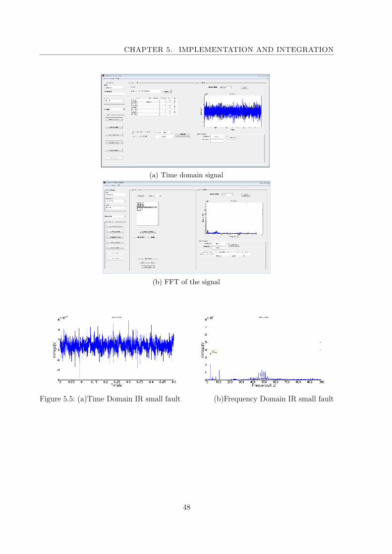
CHAPTER 5. IMPLEMENTATION AND INTEGRATION
(a) Time domain signal
(b) FFT of the signal
Figure 5.5: (a)Time Domain IR small fault (b)Frequency Domain IR small fault
48

CHAPTER 5. IMPLEMENTATION AND INTEGRATION
Figure 5.6: (a)Time Domain IR small fault (b)Frequency Domain IR small fault
Figure 5.7: (a)Time Domain OR small fault (b)Frequency Domain OR smallfault
Figure 5.8: (a)Time Domain OR heavy fault (b)Frequency Domain OR heavyfault
5.3.1.3 Feature Matrix
The features needed for the classification can be seen by switching to the feature extractionblock of navigation menu. The toolbox provides in total of 17 features, form which only therequired features are selected for the classification. The best features for the classificationcan be determined by doing feature analysis on the data. Number of columns in a feature
49

CHAPTER 5. IMPLEMENTATION AND INTEGRATION
matrix is dependent on the selected number of features. And each row of the featurematrix contains features computed for one data file as observation to classifier.
Figure 5.9: Feature Extraction
5.3.1.4 Training Data
Training data contains the folders of signals with all the fault classes, which can givento algorithm for training. This can be done by switching to the classification blockof navigation menu. Fig.5.10 shows the GUI of classification plane. The training datacontains the class names and listed files of these classes. After loading the training datafolders, the feature matrix of all the training data is computed by clicking the button’create features of all classes’.
5.3.1.5 Test Data
Test data is the folder of the fault class of unknown to be tested. This folder path can beincluded by clicking ’choose folder’ button in the testing plane of classification windowas shown in Fig.5.10 After loading the data and choosing the classifier the classificationresult can be viewed in percentage for the detected class in the table.
50

CHAPTER 5. IMPLEMENTATION AND INTEGRATION
Figure 5.10: Classification window
5.3.1.6 Classifiers
Classifiers contains the paths of all the classification algorithms. Implemented SVMfunction is included in this path.
5.4 Implementation of Muti class Support VectorMachine
Support Vector Machine (SVM) adapted for this classfication fault classes is shown inthe figure below.
51


CHAPTER 5. IMPLEMENTATION AND INTEGRATION
For the measured raw data the time domain features are calculated for every 50000samples, here the sampling frequency is 25kHz it means that features are calculated forevery 2 seconds of measured data and given as a cumulative observation for the classifier.Each row of the feature vector specifies the observation of measured samples for 2 secondsand each column represent one corresponding feature of the measured sensor data. Inthe same way a group vector is constructed for every row observation of feature vector,this string specifies the unique group name of the observation.
Figure 5.11: Preparing data set for classification
MATLAB developed code for svm classification:function [prediction] = svm(trainingmatrix,groupvector,testmatrix)%This function creates a model for the training vector with corresponding group
labels in the group vector, classifies a given test set using an SVM classifier according toa one vs. all relation.
53

CHAPTER 5. IMPLEMENTATION AND INTEGRATION
function [ p r ed i c t i o n ] = svm( t ra in ingmatr ix , groupvector , t e s tmat r i x )%This func t i on c r ea t e s a model f o r the t r a i n i n g vec t o r wi thcor re spond ing group l a b e l s in the group vec to r%c l a s s i f i e s a g iven t e s t s e t us ing an SVM c l a s s i f i e raccord ing to a one vs . a l l r e l a t i o n .
u=unique ( groupvector ) ;% s e l e c t i n g number o f c l a s s e s as l e n g t h o f unique va l u e sin group vec to r
C la s s e s=length (u ) ;%cons i de r ing l e n g t h f o r p r ed i c t e d c l a s s l a b e l s
p r ed i c t i o n = zeros ( length ( t e s tmat r i x ( : , 1 ) ) , 1 ) ;
%This f o r loop c r ea t e s k number o f svm modelswhere ’ k ’ i s no . o f f a u l t c l a s s e s
for k=1: C la s s e s%Vector i zed s ta tement t ha t b i n a r i z e s Group where1 i s the cur rent c l a s s and 0 i s a l l other c l a s s e s
OneVsAll=(groupvector==u(k ) ) ;models ( k )= svmtrain ( t ra in ingmatr ix , OneVsAll , ’ ke rne l_funct ion ’ , ’RBF ’ ) ;end
%c l a s s i f y i n g t e s t samplesfor j =1: s ize ( tes tmatr ix , 1 )
%Taking row l engh t h as no . o f t e s t i n g v a r i a b l e sfor k=1: C la s s e si f ( s vmc l a s s i f y ( models ( k ) , t e s tmat r i x ( j , : ) ) )break ;endendp r ed i c t i o n ( j ) = k ;end
When an unknown folder containing signals is given as an input for testing the model,
54

CHAPTER 5. IMPLEMENTATION AND INTEGRATION
the calculation of features is automated for this data and the model will result thepredicted group in estimated percentage
The integrated method in the toolbox is tested with all test data which containsthe folders of fault classes. After testing the data it is compared with actual data andaccuracy of the classifier is measured.
Signal Training Testing MSVM accu-racy
IR small damage 17 10 100%No damage 42 10 100%OR heavy damage 8 5 100%OR small damage 15 10 100%Ball damage 27 10 100%Total 109 (70%) 45 (30%) 100%
Table 5.3: Classification accuracy of MSVM
5.4.1 Performance Evaluation
As we have tested this model with off-line measured data, we have used CV partitionmethod in MATLAB for randomly partitioning training and test vectors in differentinstances for testing model efficiency. The classification result is 100% for the data thatis separated before the training process. In this case the data is fixed for training andtesting the data, which gives the same result if the algorithm is test for any number oftimes.
5.4.1.1 Cross Validation (CV) partitioning
This section describes the way how the data is partitioned using cross validation. Inthis implementation an intelligent way of data separation is done using the function’cvpartition’. All the files are joined into a complete data set with the corresponding groupvector containing group labels of these classes and then separated using "CV partition"function in MATLAB.Partitioning the available data into sets can reduce the number of samples which can beused for learning model and the results can depend on that particular random choice forthe pair of training and test sets.
Cross Validation gives the solution for this problem in finding the best model. In this
55
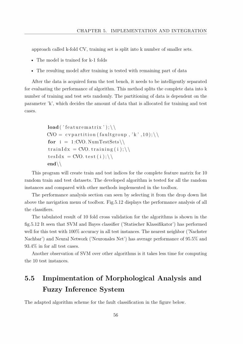
CHAPTER 5. IMPLEMENTATION AND INTEGRATION
approach called k-fold CV, training set is split into k number of smaller sets.
• The model is trained for k-1 folds
• The resulting model after training is tested with remaining part of data
After the data is acquired form the test bench, it needs to be intelligently separatedfor evaluating the performance of algorithm. This method splits the complete data into knumber of training and test sets randomly. The partitioning of data is dependent on theparameter ’k’, which decides the amount of data that is allocated for training and testcases.
load ( ’ f e a tu r emat r i x ’ ) ; \ \CVO = cvpa r t i t i o n ( fau l tgroup , ’ k ’ , 1 0 ) ; \\for i = 1 :CVO. NumTestSets\\t r a i n Idx = CVO. t r a i n i n g ( i ) ; \ \t e s Idx = CVO. t e s t ( i ) ; \ \end\\
This program will create train and test indices for the complete feature matrix for 10random train and test datasets. The developed algorithm is tested for all the randominstances and compared with other methods implemented in the toolbox.
The performance analysis section can seen by selecting it from the drop down listabove the navigation menu of toolbox. Fig.5.12 displays the performance analysis of allthe classifiers.
The tabulated result of 10 fold cross validation for the algorithms is shown in thefig.5.12 It seen that SVM and Bayes classifier (’Statischer Klassifikator’) has performedwell for this test with 100% accuracy in all test instances. The nearest neighbor (’NachsterNachbar’) and Neural Network (’Neuronales Net’) has average performance of 95.5% and93.4% in for all test cases.
Another observation of SVM over other algorithms is it takes less time for computingthe 10 test instances.
5.5 Impimentation of Morphological Analysis andFuzzy Inference System
The adapted algorithm scheme for the fault classification in the figure below.
56


CHAPTER 5. IMPLEMENTATION AND INTEGRATION
A tool is developed for doing morphological operations on the given input signal. Thistool outputs the actual FFT plot of the signal and three gradient operators obtained bymorphologically filtering the signal. It has two input parameters
• RPM: Rotation per minute numerical value of the the machinery to be tested.
• fault freq: This specifies the threshold fault frequency, detecting fault should bebelow this value.
5.5.1 Morphological Analysis (MA)
Vibration signal is given as input to the function along with the parameters ’RPM’, ’faultfr’ as shown in fig.?? The length of the signal can be indefinite, sampling frequency 25Khz is preset inside the function. Ten Structuring Elements (SE’s) of different lengthsare created based on ’fault fr’ input and the best of it selected which has highest kurtosisvalue.
Morphological gradients are computed for all the samples of the vibration signalwith the SE chosen upon kurtosis value. The function outputs the impulses of the inputvibration signal as ’frequency peaks’. Later this array of containing peaks are given asinput to Fuzzy Inference System (FIS).Selection of SE:
SE is one of the determinative factor for morphological operation, which has asignificant effect on the result. In general, only when the scale and shape of the signalare matched to those of SE, the signal will be reserved. Therefore, the shape,height(amplitude) and length (domain) of SE should be selected accordingly to the signal to beanalyzed.
In our work, flat SEs (height=1) are chosen. Research shows that shape of SE willhave little effect on the analysis. Length of the SE is crucial.If we consider much shorterlength, much more impulse features will be extracted, while much noise will be retainedin the signal, this makes the demodulation of the signal to be difficult. If we considerwith larger length, less impulse features will be extracted, and some useful informationwill be reserved.A kurtosis based criterion is used for the selection of length of SE.
The obtained signal data from the test bench can be morphologically filtered withten different SEs with different lengths spaced by 10% of the pulse repetition values. Thepulse repetition value (T) is the pulse period from either the Inner Ring (IR) or OuterRing (OR) fault. The kurtosis of the morphologically filtered signals are calculated, thesevalues give an approximate estimate of the peaks present in the signal. Therefore, the
58
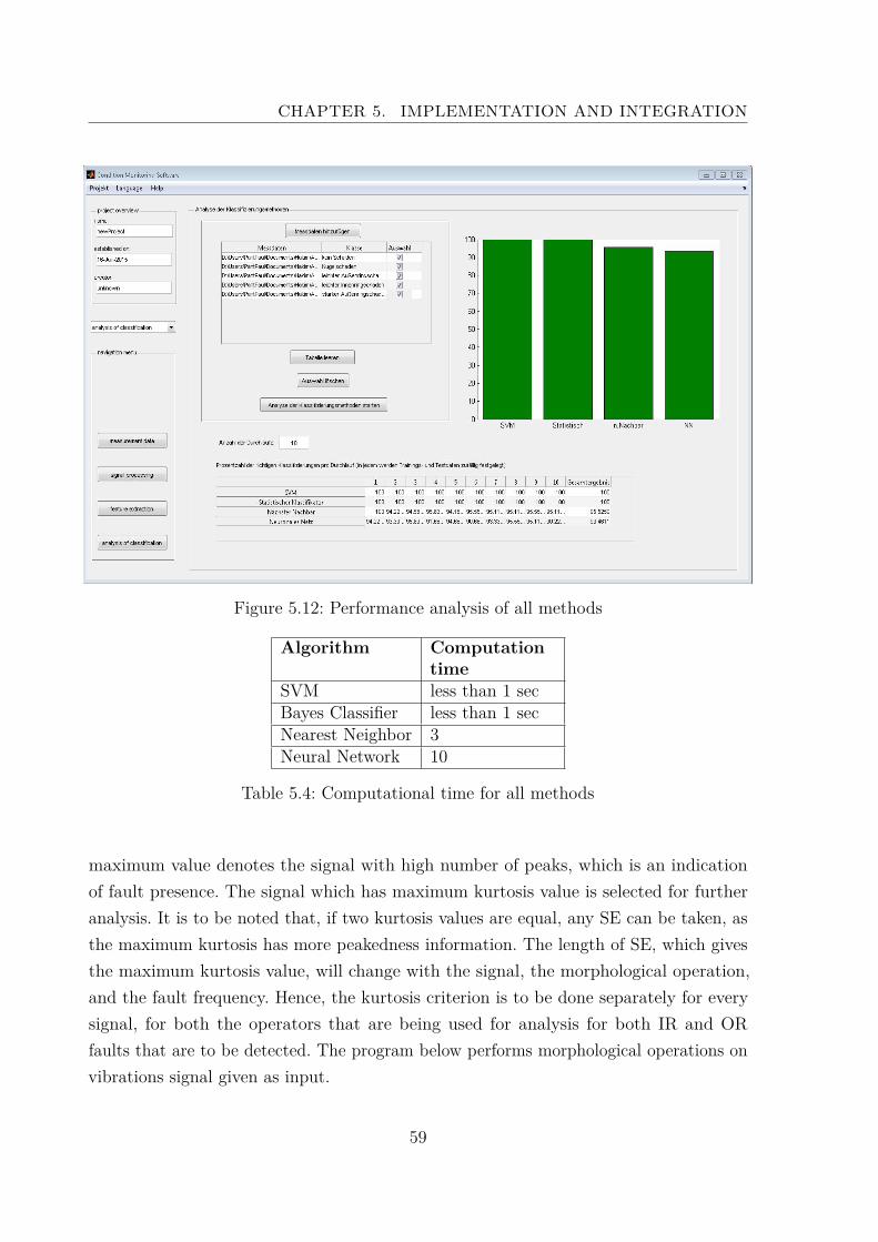
CHAPTER 5. IMPLEMENTATION AND INTEGRATION
Figure 5.12: Performance analysis of all methods
Algorithm Computationtime
SVM less than 1 secBayes Classifier less than 1 secNearest Neighbor 3Neural Network 10
Table 5.4: Computational time for all methods
maximum value denotes the signal with high number of peaks, which is an indicationof fault presence. The signal which has maximum kurtosis value is selected for furtheranalysis. It is to be noted that, if two kurtosis values are equal, any SE can be taken, asthe maximum kurtosis has more peakedness information. The length of SE, which givesthe maximum kurtosis value, will change with the signal, the morphological operation,and the fault frequency. Hence, the kurtosis criterion is to be done separately for everysignal, for both the operators that are being used for analysis for both IR and ORfaults that are to be detected. The program below performs morphological operations onvibrations signal given as input.
59
CHAPTER 5. IMPLEMENTATION AND INTEGRATION
fault_tym=1/ f au l t_ f r ;X=25000∗ fault_tym ;
%for t a k ing d i f f e r e n t S t ruc tu re Element l e n g t h sXk=[0.1∗X 0.2∗X 0.3∗X 0.4∗X 0.5∗X 0.6∗X 0.7∗X 0.8∗X 0.9∗X 1∗X] ;Xk=round(Xk ) ; i =1;clear d i l 1 erd1 grad∗ s i g_f k f r e q ∗ max∗ peak ∗ ;
for X1=Xkclear se ;% crea t i n g S t ruc tu r ing Elementsse=s t r e l ( ones (X1 , 1 ) ) ;d i l 1 ( i , : )= imd i l a t e ( s ig , se ) ;erd1 ( i , : )= imerode ( s ig , se ) ;
grad1 ( : , i )= imd i l a t e ( s ig , se )− imerode ( s ig , se ) ; % Beucher g rad i en tgrad2 ( : , i )= imc lo se ( s ig , se )−imopen ( s ig , se ) ; % Se l f contemporary hat% c a l c u l a t i n g k u r t o s i s va lue f o r s e l e c t i o n o fSE form 10 d i f f e r e n t SE usedk ( i ,1)= ku r t o s i s ( grad1 ( : , i ) ) ; k ( i ,2)= ku r t o s i s ( grad2 ( : , i ) ) ;%k ( i ,3)= ku r t o s i s ( grad3 ( : , i ) ) ;
i=i +1;end[ a , b]= sort ( k ) ;
% For p l o t t i n g graphsN=32768;Fs=25000;T=N/Fs ; f req_s =(0:N−1)/T;% f i g u r e ( ) ;s i g_f=abs ( f f t ( s i g ( 1 :N) ,N) ) ;%subp l o t ( 2 , 2 , 1 ) ;plot ( f req_s ( 1 : 5 5 0 ) , s i g_f ( 1 : 5 5 0 ) ) ; t i t l e ( ’ s i g n a l ’ ) ;grad1_f=abs ( f f t ( grad1 ( 1 :N, b ( 10 , 1 ) ) ,N) ) ;%subp l o t ( 2 , 2 , 2 ) ;plot ( grad1_f ( 1 : 5 5 0 ) ) ; t i t l e ( ’ besucher ’ ) ;subplot ( 2 , 2 , 3 ) ; plot ( grad2_f ( 1 : 5 5 0 ) ) ;
60

CHAPTER 5. IMPLEMENTATION AND INTEGRATION
t i t l e ( ’ s e l f ␣ contemporarys ␣ top␣hat ’ ) ;
%Finding Frequency peaks in Gradient 1[ c , d]= sort ( grad1_f ( 1 : 5 5 0 ) , 1 , ’ descend ’ ) ;
for i =1:10max_f_grad1 ( i )=freq_s (d( i +1)) ;% peak_freq_1 ( i )=freq_1 (d ( i +1));
end
5.5.2 Fuzzy Inference System (FIS)
The mamdami fuzzy is chosen from fuzzy tool box of MATLAB. Both input and outputmembership functions are chosen as triangular shaped (’trimf’). Three input membershipfunctions are defined over the ranges of the fault classes, which are calculated theoretically.The output membership functions are fault classes with ranges from 0 to 1, this specifiesthe degree of belief for that damage. The fuzzy classifier ouputs the class label which iscloser to 1. If then rules are formulated.
For example when the frequency peaks are given as input the looks for the membershipfunctions where these peaks come under and the if-then rule knowledge given to fuzzycomputes the out membership function degree. Fig.5.13 shows the formulation of fuzzyrules to the membership functions defined.
The classification results for the vibration with determined impuses are shown in Fig
61

CHAPTER 5. IMPLEMENTATION AND INTEGRATION
Figure 5.13: Fuzzy rules for fault classification
Figure 5.14: Detected frequency peak of IR fault
62

CHAPTER 5. IMPLEMENTATION AND INTEGRATION
Figure 5.15: Detected frequency peak of OR fault
5.6 Summary
• Two different approached namely multi class support vector machine (MSVM) andmorphological analysis and fuzzy inference system (MAFIS) are implemented forthe condition monitoring of roller bearing
• The performance of implemented analytical approach SVM is compared with theother methods.
• The classification accuracy is 100% because the data can be linearly separable forthe selected features. This shows that the features chosen are good for classification.
• This performance analysis is carried out by cross validation partitioning of thewhole data set wherein the the whole dataset is randomly chosen for 10 instances.The classification accuracy for all these instances is computed.
• The advantage of cross validation is that the best model for the classification isdetermined from a set of disposed models.
63

Ch
ap
te
r 6Embedded Implementation
6.1 Development Board
After doing the market analysis, there are three major platforms which suit for thisapplication. The table illustrates the features of the these different platforms.
Specification Raspberry pi Raspberry pi 2 UdooArchitecture 32 bit ARM 700 MHz 32 bit Quadcore ARM
Cortex-A7 900 MHz32 bit Cortex-A9Quadcore 1GHz
RAM 512 MB DDR3 1 GB DDR3 1 GB DDR3OS Linux Linux,Windows LinuxGPIO’s 17 available 40 available 76 availableUSB X X XSPI X X XI2c X X XProgramming C,C++,MATLAB,
PythonC,C++,MATLAB,Python
C,C++,Python
Price 25e 40e 110e
Table 6.1: Market analysis on different development boards
For building an embedded system one must follow this paradigm: Developed algorithmsare tested on host pc and the best performing algorithm should be deployed intohardware. In order to deploy the standalone application on embedded system the followingrequirements has to be fulfilled:
64

CHAPTER 6. EMBEDDED IMPLEMENTATION
• It should meet the memory constraints for the developed algorithm.
• It should have good support from MATLAB in developing standalone for embeddedto speed up the deployment process.
We have chosen Raspberry pi 2 for our application prototyping, as it has a powerfulARM v7 quad core processor with a clock speed of 900 MHz. The main reason forchoosing this board as it is highly customizable and all the framework developed for itsearlier version is compatible for this newer version.
The main idea in deploying this concept into embedded hardware is to reduce thecost and also to make this system real time in capturing the machine condition. Thisdeveloped hardware has following features:
• Wireless communication form a host PC for measuring and accessing the data
• Condition monitoring is done through a efficient algorithm, which is tested on hostPC
The table gives the cost comparison between developed hardware and traditional approachusing industrial sensors.
Developed hardware Conventional methodSensor 2.50e Sensor 2000eSensor eval board 20e Data logger board 1500eRaspberry pi 2 Board 40e Lab viewWifi Module 9e MiscellaneousConnecting wires 5e othersPrice 79e Price 4000e
Table 6.2: Cost comparison between proposed approach and conventional approach
The advantage of developed hardware is that it be used for both data extraction andon board condition monitoring.
6.2 MEMS Vibration Sensor
There are wide variety of sensors available for the measurement of acceleration on themarket, it is important to choose right sensor for the application . The selected sensor
65

CHAPTER 6. EMBEDDED IMPLEMENTATION
should capture the damage frequencies, for this it has output rate double the range ofdamage frequencies as per the Nyquist criterion.
The selected sensor has to meet the following requirements:
• Output rate greater than 3 kHz
• Digital Interface(SPI,I2C)
• Small size
• Low cost
The table shows various sensors that are available in the market
Sensor Operating Fre-quency[Hz]
Acceleration[m/s2]
Interface Size[mm] Cost
ADXL345BCCZ 3200 3 x 160 SPI 5 4.80eLIS3DH 5000 3 x 160 SPI 3 2.50eBU-21771-000 3000 1 x Vibration Analog 8 85eADIS16227CMLZ 100000 3 x 700 SPI 15 70eADXL001-70 22000 1 x 700 Analog 5 28eMMA6825BKW 1000 2 x100 SPI 6 9.50eBMA280 500 3 x 160 SPI 3 0.85eADXL345BCCZ 3200 3 x 160 SPI 5 4.80e
Table 6.3: Market analysis for different MEMS sensors
From the analysis LIS3DH fits best as per the requirements, It’s has good outputfrequency and also less in price.
6.3 Preparing Raspberry
Initially the board is connected to the sensor using I2c interface, but this has limitationin recording the data. Later SPI interface is used to increase the data logging speed. Thepin layout of the raspberry pi 2 is shown in Fig
6.3.1 Sensor Interface
Raspberry pi 2 comes with micro SD card slot. RASPBIAN (Debian Wheezy) operatingsystem can be downloaded and flashed into sd card. Once the SD card is inserted intothe board and powered on, the following default login credentials are used after the bootscreen.
66

CHAPTER 6. EMBEDDED IMPLEMENTATION
• Username pi
• Password raspberry
The following procedure is used for enabling the I2C and SPI communication withthe peripheral devices. The command sudo rasp-config is used to get into raspberry piconfiguration window.
Figure 6.1: Raspberry pi configuration menu
Enable SPI,I2C,SSH through advanced options. After enabling the board needs toreboot and command startx is used to jump into RASPBIAN desktop graphical interface.
6.3.2 I2C Communication
Here we have LIS3DH sensor embedded on STEVAL-MKI105V1 adapter board. Theconnection between board and the raspberry are done accordingly with the pin descriptionon the board. The pin connections of the sensor to the board are given in the table.
The register addresses of the connected I2C Peripherals can be accessed by usingcommand sudo i2cdetect -y 1 or sudo i2cdetect -y 0.
67

CHAPTER 6. EMBEDDED IMPLEMENTATION
Sensor board I2C pins Rasp-berry
CS Pin 24SCL Pin 23SDA Pin 19SDO Pin -GND Pin 39VCC Pin 01
Table 6.4: SPI pin connectivity between raspberry and LIS3DH
The Fig shows LIS3DH sensor is detected on register 0X19. A python program iswritten to access the data form the sensor. The functions required to access the registerdata are included in SMBUS package of python, this can be downloaded and importedin the program. LI3DH sensor manufacturer data sheet has register mapping details toenable the registers for sensor data acquisition. A simple python script is written toenable the registers and get the 3 axes data from the sensor.
The sensor output has two’s compliment output for each axis. This can be convertedinto acceleration value by logical shift operation and combining low and high value ofeach axis. A Linux shell script is written to log the printed acceleration data output ofpython program into a text file, later this can be analyzed in MATLAB. But the mainproblem is that it limits the data recording to 700 Mhz sampling frequency. This can beovercomed by switching to SPI protocol
68
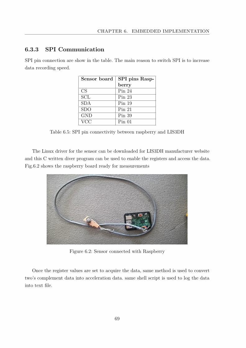
CHAPTER 6. EMBEDDED IMPLEMENTATION
6.3.3 SPI Communication
SPI pin connection are show in the table. The main reason to switch SPI is to increasedata recording speed.
Sensor board SPI pins Rasp-berry
CS Pin 24SCL Pin 23SDA Pin 19SDO Pin 21GND Pin 39VCC Pin 01
Table 6.5: SPI pin connectivity between raspberry and LIS3DH
The Linux driver for the sensor can be downloaded for LIS3DH manufacturer websiteand this C written diver program can be used to enable the registers and access the data.Fig.6.2 shows the raspberry board ready for measurements
Figure 6.2: Sensor connected with Raspberry
Once the register values are set to acquire the data, same method is used to converttwo’s complement data into acceleration data. same shell script is used to log the datainto text file.
69
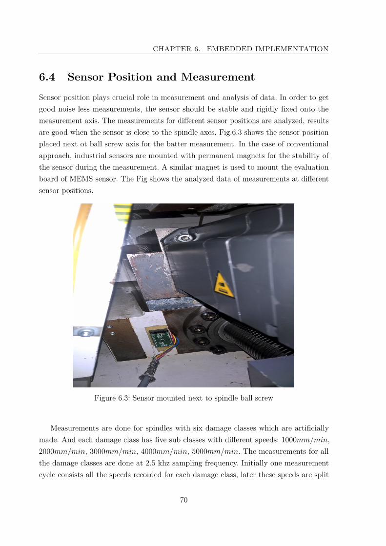
CHAPTER 6. EMBEDDED IMPLEMENTATION
6.4 Sensor Position and Measurement
Sensor position plays crucial role in measurement and analysis of data. In order to getgood noise less measurements, the sensor should be stable and rigidly fixed onto themeasurement axis. The measurements for different sensor positions are analyzed, resultsare good when the sensor is close to the spindle axes. Fig.6.3 shows the sensor positionplaced next ot ball screw axis for the batter measurement. In the case of conventionalapproach, industrial sensors are mounted with permanent magnets for the stability ofthe sensor during the measurement. A similar magnet is used to mount the evaluationboard of MEMS sensor. The Fig shows the analyzed data of measurements at differentsensor positions.
Figure 6.3: Sensor mounted next to spindle ball screw
Measurements are done for spindles with six damage classes which are artificiallymade. And each damage class has five sub classes with different speeds: 1000mm/min,2000mm/min, 3000mm/min, 4000mm/min, 5000mm/min. The measurements for allthe damage classes are done at 2.5 khz sampling frequency. Initially one measurementcycle consists all the speeds recorded for each damage class, later these speeds are split
70

CHAPTER 6. EMBEDDED IMPLEMENTATION
Figure 6.4: Measured data- Sensor Position far from spindle
Figure 6.5: Measured data- Sensor Position closer to spindle
into five sub classes for the analysis. The measurement cycle recorded with 5 differentspeeds is shown in fig.6.6
After partitioning the fault damage classes form the measurement they can be usedto analyze on Condition Monitoring tool developed in MATLAB. These measurementsare compared with measurements done using industrial sensor (Conventional Approach).Feature matrix is generated and Fig. shows features space comparison between MEMSsensor and Industrial sensor.
71

CHAPTER 6. EMBEDDED IMPLEMENTATION
Figure 6.6: Signal split for different speeds
6.5 Suppor Vector Machine Implementation onRaspberry Pi
The idea is to deploy SVM on a embedded hardware for ensuring real time conditionmonitoring.
6.5.1 Development Environment
The MATLAB developed script cannot be deployed on Raspberry pi 2. Using pythonon the raspbian wheezy OS for the algorithm development is the best available solution.In contrast to toolboxes in MATLAB different packages are available in python withdeveloped frameworks. Once the packages are downloaded, they can be imported to theprogram in performing specific functions. the list of packages needed for this project andtheir use given the table below
"sudo apt-get install python-smbus" installs smbus package, In the same way ’smbus’is replaced with other package names to install them on raspberry[22]. The package’scikit-learn’ contains frame work developed for many Machine Learning (ML) algorithms,these algorithms can be used to develop solving problems such as classification, regression,clustering similar to ML tool box in MATLAB. SVM classification function can usedfrom this package for the implementation.
72

CHAPTER 6. EMBEDDED IMPLEMENTATION
Packages RequirementNumPy For scientific
computingSciPy For mathemati-
cal oprationsscikit-learn Machine Learn-
ing PythonSMBUS For I2C commu-
nication
Table 6.6: Package required for Python on raspberry
6.6 Evaluation of Spindle Data
The measured data from the MEMS sensor is spited according to speeds and stored indifferent folders as shown in Fig.6.7 for the preparation dataset.
Figure 6.7: Folder structure on Raspberry
The dataset is computed as similar to roller bearing, Which is illustrated Fig.5.11 inthe chapter 5. Each fault class with different speed has different class label. In total thereare 6 fault classes with 5 different speeds, which constitute 30 individual class labels. Fortesting the algorithm these fault classes are tested for all speeds separately to capturethe dynamic behavior of the spindle.
73

CHAPTER 6. EMBEDDED IMPLEMENTATION
The python script[] is developed for the calculation of feature vectors for these damageclasses and plot them in 3D space. The calculated features spread over 3D space can beviewed.
Figure 6.8: 3D feature space of faults at 1000 mm/min speed
Figure 6.9: 3D feature space of faults at 2000 mm/min speed
74

CHAPTER 6. EMBEDDED IMPLEMENTATION
Figure 6.10: 3D feature space of faults at 3000 mm/min speed
Figure 6.11: 3D feature space of faults at 4000 mm/min speed
75
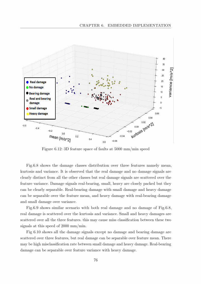
CHAPTER 6. EMBEDDED IMPLEMENTATION
Figure 6.12: 3D feature space of faults at 5000 mm/min speed
Fig.6.8 shows the damage classes distribution over three features namely mean,kurtosis and variance. It is observed that the real damage and no damage signals areclearly distinct from all the other classes but real damage signals are scattered over thefeature variance. Damage signals real-bearing, small, heavy are closely packed but theycan be clearly separable. Real-bearing damage with small damage and heavy damagecan be separable over the feature mean, and heavy damage with real-bearing damageand small damage over variance.
Fig.6.9 shows similar scenario with both real damage and no damage of Fig.6.8,real damage is scattered over the kurtosis and variance. Small and heavy damages arescattered over all the three features. this may cause miss classification between these twosignals at this speed of 2000 mm/min.
Fig 6.10 shows all the damage signals except no damage and bearing damage arescattered over three features, but real damage can be separable over feature mean. Theremay be high misclassification rate between small damage and heavy damage. Real-bearingdamage can be separable over feature variance with heavy damage.
76
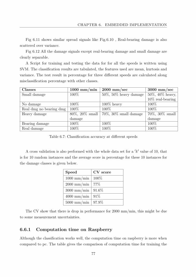
CHAPTER 6. EMBEDDED IMPLEMENTATION
Fig 6.11 shows similar spread signals like Fig.6.10 , Real-bearing damage is alsoscattered over variance.
Fig 6.12 All the damage signals except real-bearing damage and small damage areclearly separable.
A Script for training and testing the data for for all the speeds is written usingSVM. The classification results are tabulated, the features used are mean, kurtosis andvariance. The test result in percentage for three different speeds are calculated alongmisclassification percentage with other classes.
Classes 1000 mm/min 2000 mm/sec 3000 mm/secSmall damage 100% 50%, 50% heavy damage 50%, 40% heavy,
10% real-bearingNo damage 100% 100% heavy 100%Real dmg no bearing dmg 100% 100% 100%Heavy damage 80%, 20% small
damage70%, 30% small damage 70%, 30% small
damageBearing damage 100% 100% 100%Real damage 100% 100% 100%
Table 6.7: Classification accuracy at different speeds
A cross validation is also performed with the whole data set for a ′k′ value of 10, thatis for 10 random instances and the average score in percentage for these 10 instances forthe damage classes is given below.
Speed CV score1000 mm/min 100%2000 mm/min 77%3000 mm/min 91.6%4000 mm/min 91%5000 mm/min 97.9%
The CV show that there is drop in performance for 2000 mm/min, this might be dueto some measurement uncertainties.
6.6.1 Computation time on Raspberry
Although the classification works well, the computation time on raspberry is more whencompared to pc. The table gives the comparison of computation time for training the
77

CHAPTER 6. EMBEDDED IMPLEMENTATION
data between pc and raspberry.
speed PC trainingtime [sec]
Raspberry training time [sec] classes
1000 8.7779 137.4732 62000 5.5842 81.9726 63000 3.866 52.2472 64000 3.1706 40.2787 65000 3.0629 38.9367 6
Table 6.8: Computation speed comparison between pc and raspberry pi for 6 features
speed PC trainingtime [sec]
Raspberry training time [sec] classes
1000 8.4775 137.3145 62000 5.4367 81.4436 63000 3.8041 51.8508 64000 3.1384 39.7422 65000 3.0335 38.5836 6
Table 6.9: Computation speed comparison between pc and raspberry pi for 3 features
6.7 Summary
• The proposed concept performs well on condition monitoring tool. The idea ofprototyping algorithms like SVMmethods on a embedded hardware for the conditionmonitoring is discussed in this chapters.
• For this evaluation a LIS3DH MEMS sensor and Raspberry pi 2 hardware is chosen.And the proposed algorithm developed on Python environment.
• Data acquisition for a spindle is done to its dynamic behavior for speeds rangingform 1000 mm/sec to 5000 mm/sec.
• Classification test is performed for different fault classes of spindle and their resultsare tabulated. According the computation time for this method is compared forboth PC and Raspberry.
78

Ch
ap
te
r 7Conclusion and Future Work
In this work, two different approaches for the early fault diagnosis of machine toolcomponents are investigated and implemented. The first approach is analytical in natureand uses support vector machine (SVM) which has its foundations in statistical learningtheory. The second approach is knowledge based, namely morphological analysis withfuzzy inference system (MAFIS). These methods use vibrational data from two differentmachine tool components; the roller bearings and the spindle.
The major difference between MAFIS and SVM based approach is that MAFISutilizes a priori knowledge (geometry of the roller bearings) and then fuzzy inferencesystem (FIS) will use this knowledge to predict the class labels. On the other hand SVMlearns directly from the training data which has to be first acquired from the machinesspindle to determine the spread of feature space for different class labels. Thus in casethe components are replaced MAFIS can work while the SVM needs to be retrained withnew data.
Additionally, the advantage of using SVM approach is it can easily work with any nonlinear system without the need of modelling the system first. The developed SVM formultiple fault classes classification is tested and integrated into the condition monitoringtool at Fraunhofer IPK. Performance analysis is carried on all methods in the toolusing cross validation (CV) for the whole data. The results of this test shows the SVMexhibits higher accuracy with lesser computation cost. This better functioning algorithmis prototyped on raspberry pi hardware for the condition monitoring of a spindle.
79

CHAPTER 7. CONCLUSION AND FUTURE WORK
The results of SVM on raspberry are shown and the main concern is the computationalcost during training. The training of developed SVM in Python environment on raspberrypi takes more time than PC. But the raspberry pi with SVM is cost effective for thecondition monitoring of machine tool components. On the other hand the conventionalapproach in industries make use different hardware for data acquisition and differentenvironment for the processing of signal which is very expensive way of doing.
Future work:
The developed hardware can be extended to support warning system wherein ononset of a fault the system reports to the user over the web.
Another idea is to deploy multiple sensor nodes for the condition monitoring toolchain of different components in a big machinery plant and make all these nodes tointeract through wireless communication with the master node. Here each and everynode is equipped with all the necessary components needed for fault diagnosis.Thisapproach allows industries to reach the goal of more efficient and cost effective intelligentmaintenance system.
80

Bibliography
[1] J.H. WilliamsCondition-based Maintenance and Machine Diagnostics [page 11]
[2] Pierre TchakouaWind Turbine Condition Monitoring: State-of-the-Art Review, New Trends, and
Future ChallengesEnergies 2014, 7, 2595-2630; doi:10.3390/en7042595
[3] Hongyu Yang Vibration Feature Extraction Techniques for Fault Diagnosis of RotatingMachinery Asia- Pacific Vibration Conference, 12-14 November 2003, Gold Coast,Australia.
[4] Tshilidzi MarwalaCondition Monitoring Using Computational Intelligence MethodsISBN 978-1-4471-2379-8
[5] Xiang Gong University of Nebraska-LincolnONLINE NONINTRUSIVE CONDITION MONITORING AND FAULT DETEC-
TION FOR WIND TURBINES
[6] Temperature dependent friction estimation: Application to lubricant health monitoringMechatronics 22 (2012) 1078–1084
[7] S. BagavathiappanInfrared thermography for condition monitoring – A reviewInfrared Physics and Technology 60 (2013) 35–55
[8] D. Mba and Raj B. K. N. RaoDevelopment of Acoustic Emission Technology for Condition Monitoring and Diagno-
sis of Rotating Machines: Bearings, Pumps, Gearboxes, Engines, and RotatingStructures
81

BIBLIOGRAPHY
The Shock and Vibration Digest 01/2006; 38(1):3-16. DOI: 10.1177/0583102405059054
[9] @onlineCondition Monitoring within a Reliability Context,url = http://algoengines.com/condition-monitoring-in-time-and/, OPTsubtitle =
Condition Monitoring
[10] Abhinay V. DubeVibration Based Condition Assessment Of Rollingelement Bearings With Local-
ized Defects. INTERNATIONAL JOURNAL OF SCIENTIFIC TECHNOLOGYRESEARCH VOLUME 2, ISSUE 4, APRIL 2013.
[11] A new structuring element for multi-scale morphology analysis and its applicationin rolling element bearing fault diagnosis
Journal of Vibration and Control 0(0) 1–25 The Author(s) 2013
[12] A. Santhana Raj and N. MuraliEarly Classification of Bearing Faults Using Morphological Operators and Fuzzy
InferenceIEEE TRANSACTIONS ON INDUSTRIAL ELECTRONICS, VOL. 60, NO. 2,
FEBRUARY 2013
[13] S. B. KotsiantisSupervised Machine Learning: A Review of Classification TechniquesInformatica 31 (2007) 249-268
[14] Achmad WidodoSupport vector machine in machine condition monitoring and fault diagnosisMechanical Systems and Signal Processing 21 (2007) 2560–2574
[15] Christian Weiss, Holger Frohlich and Andreas Zell Department of Computer ScienceVibration-based Terrain Classification Using Support Vector Machines.
[16] Julian VitayAI lab, Dept. of computer science, Tu Chemnitz @bookletSVM-Machine learn-
ing,Chapter 5-SVM
[17] Isabella GuyonAn Introduction to Feature Extraction
[18] Fuzzy Systems Toolbox, M. Beale and H DemuthPractical Implementation of a fuzzy inference system:examples
82

BIBLIOGRAPHY
[19] Eckart Uhlmann,Abdelhakim LaghmouchiConfigurable Condition Monitoring Methods for Industrial Product Service Systems.
[20] HOSSEIN A. ESTILAFBEARING FAULT DIAGNOSIS OF ELECTRICAL MACHINE BASE ON VIBRA-
TION SIGNAL USING MULTI-CLASS SUPPORT VECTOR MACHINEIndian J.Sci.Res.. 2(1) : 46-53, 2014 ISSN :
[21] Jeevanand S, Member IEEEState of Art on Condition Monitoring of Induction Motors
[22] @onlinePhysical computing with Raspberry Pi,url = https://www.cl.cam.ac.uk/projects/raspberrypi/tutorials/robot/downloads/,
OPTsubtitle = Installing extra packages
[23] @onlineCondition Monitoring within a Reliability Context,url = http://www.lifetime-reliability.com/free-articles/maintenance-
management/condition-monitoring-as-a-reliability-improvement-strategy.html,OPTsubtitle = Condition Monitoring
[24] Vibration Based Condition Assessment Of Rollingelement Bearings With LocalizedDefects
INTERNATIONAL JOURNAL OF SCIENTIFIC and TECHNOLOGY RESEARCHVOLUME 2, ISSUE 4, APRIL 2013
[25] A Generic Data Processing Framework for Heterogeneous Sensor-Actor-Networks.Matthias Vodel, Rene Bergelt, and Wolfram HardtDept. of Computer Science Chemnitz University of TechnologyInternational Journal on Advances in Intelligent Systems, vol 5 no 3 & 4, year 2012
83