Concurrency Preserving Partitioning Algorithm...

VLSI DESIGN1999, Vol. 9, No. 3, pp. 253-270Reprints available directly from the publisherPhotocopying permitted by license only

(C) 1999 OPA (Overseas Publishers Association) N.V.Published by license under

the Gordon and Breach SciencePublishers imprint.

Printed in Malaysia.

Concurrency Preserving Partitioning AlgorithmParallel Logic Simulation

HONG K. KIM and JACK JEAN*

Department of Computer Science and Engineering, Wright State University, Dayton, Ohio 45435, USA

(Received 26 May 1998)

A partitioning algorithm for parallel discrete event gate-level logic simulations isproposed in this paper. Unlike most other partitioning algorithms, the proposedalgorithm preserves computation concurrency by assigning to processors circuit gatesthat can be evaluated at about the same time. As a result, the improved concurrencypreserving partitioning (iCPP) algorithm can provide better load balancing throughoutthe period of a parallel simulation. This is especially important when the algorithm isused together with a Time Warp simulation where a high degree of concurrency can leadto fewer rollbacks and better performance. The algorithm consists of three phases andthree conflicting goals can be separately considered so to reduce computationalcomplexity.To evaluate the quality of partitioning algorithms in terms of preserving concurrency,

a concurrency metric that requires neither sequential nor parallel simulation isproposed. A levelization technique is used in computing the metric so to determinegates which can be evaluated at about the same time. A parallel gate-level logicsimulator is implemented on an INTEL Paragon and an IBM SP2 to evaluate theperformance of the iCPP algorithm. The results are compared with several otherpartitioning algorithms to show that the iCPP algorithm does preserve concurrencypretty well and reasonable speedup may be achieved with the algorithm.

Keywords: Parallel logic simulation, partitioning algorithm, discrete event simulation, concur-rency, load balancing, time warp

1. INTRODUCTION

Logic simulation is a primary tool for validationand analysis of digital circuits. To reduce thesimulation time of large circuits, parallel logicsimulation has attracted considerable interest in

recent years [1]. As in many other parallelsimulations, a good partitioning algorithm is akey to achieve good performance in parallel logicsimulation, especially since the event granularity isrelatively small compared to other types ofsimulations. Partitioning algorithms can usually

* Corresponding author. Tel." 937-775-5106, Fax: 937-775-5133; e-mail: {hkim,jjean}@cs.wright.edu

253

254 H.K. KIM AND J. JEAN

be classified into two categories: static anddynamic. Static partitioning is performed prior tothe execution of the simulation and the resultingpartition is fixed during the simulation. A dynamicpartitioning scheme attempts to keep systemresources busy by migrating computation pro-cesses during the simulation. Since dynamicpartitioning involves a lot of communicationoverhead [16], static partitioning is considered inthis paper.A good partitioning algorithm is expected to

speed up parallel simulations. This may beachieved by focusing on three competing goals:to balance processor workload, to minimizeinterprocessor communication and synchroniza-tion, and to maximize concurrency. Among thosegoals, the maximization of concurrency is mostlyoverlooked by previous partitioning algorithmsfor logic simulation. Maximizing concurrencymeans partitioning a circuit such that at any timeinstance as many independent logic gates as

possible are assigned to different processors. Thiscan be achieved if workload is balanced among theprocessors all the time. However, most previousalgorithms balance the accumulated amount ofworkload over the whole simulation period insteadof the workload at any time instance.The improved concurrency preserving partition-

ing (iCPP) algorithm proposed in this paper forparallel logic simulation takes the above threegoals into consideration. It achieves a goodcompromise with a high degree of concurrency, abalanced workload, and reasonable amount ofinterprocessor communication. The compromiseleads to a significant speedup obtained with a TimeWarp parallel logic simulator implemented on anIntel Paragon and an IBM SP2. In Section 2,previous partitioning works in parallel logicsimulation are summarized. Section 3 describesthe rationale and the three phases of the proposedalgorithm. A concurrency metric is proposed inSection 4 for the evaluation of partitioningalgorithms. The algorithm is evaluated and com-

pared to several other algorithms in Section 5.Section 6 concludes the paper.

2. PREVIOUS WORKS

A number of partitioning algorithms have beenproposed for circuit simulations with slightlydifferent emphasis. The iterative improvementalgorithms perform a sequence of bi-partitioning.During each bi-partitioning, either a vertex ex-

change scheme or a one-way vertex movingscheme is used to iteratively reduce the interpro-cessor communication subject to some constraintson processor workload [7, 13]. In [23], Sanchisapplied iterative improvements to multiple-waypartitioning with a more frequent informationupdating after each vertex exchange or movingand obtained better results. Nandy and Loucksapplied this iterative improvements to the initialrandom partitioning for the parallel logic simula-tion [22]. Sanchis’s algorithm is adapted and usedin the third phase of the algorithm proposed in thispaper.To achieve a compromise between interproces-

sor communication and processor load balancing,simulated annealing may be used for partitioning[3, 10]. However, methods based on simulatedannealing are usually slow, especially when highquality solutions are to be found.

Partitioning algorithms such as the cone parti-tioning method or the Corolla method are basedon clustering techniques [4, 20, 21, 24, 26]. Thesealgorithms consist of two phases: a fine grainedclustering phase and an assignment phase. In thefirst phase, clustering is performed to increasegranularity. In the second phase, clustersare assigned to processors so to either reduceinter-processor communication or achieve loadbalancing.A problem with most previous partitioning

algorithms is that they do not produce a highdegree of concurrency [5]. They usually try tobalance the accumulated workload instead oftrying to balance the instantaneous workload. Thisleads to performance degradation caused by roll-backs when a Time Warp parallel simulation isperformed. Two exceptions are the randompartitioning which has a good chance of producing

PARALLEL LOGIC SIMULATION 255

a high degree of concurrency and the stringpartitioning [17] which did take concurrency intoaccount. However, either one tends to generate alarge amount of interprocessor communication[24]. The proposed iCPP algorithm is designed totake concurrency into consideration and achieve agood compromise among the different competinggoals.

3. PARTITIONING ALGORITHM

For partitioning purposes, a circuit may berepresented as a directed graph, G(V, E), whereV is the set of nodes, each denoting a logic gate ora flip-flop, and E E (V x V) is the set of directededges between nodes in V. Three special subsets ofV are/, O, and D, representing the set of primaryinput nodes, the set of primary output nodes, andthe set of flip-flop nodes, respectively. Severalassumptions are made in this paper regarding acircuit graph.

1. For each node, the in-degree and the out-degreeare bounded by a constant. This assumptioncorresponds to the finite amount of fan-ins andfan-outs of logic gates in a circuit.

2. Associated with each node vi, there is an activitylevel, ai, that denotes the estimated number ofevents to be simulated for the node.

3. Associated with each edge ei, there is an edgeweight, wi, that denotes the estimated numberof events to be sent over the edge.

Note that both activity levels and edge weightsmay be obtained through circuit modeling orthrough pre-simulation [6]. They are assumed tobe unity when neither modeling nor pre-simulationis attempted. Another point to mention is that thegraph may contain cycles due to the existence offlip-flops.The partitioning algorithm proposed in this

paper assigns nodes in a directed graph toprocessors of an asynchronous multiprocessor. Itconsists of three phases so that conflicting goalsmay be considered separately and computational

complexity may be reduced. For a graph with [VInodes these three phases are as follows.

Phase 1: Divide a graph into a set of disjointedsubgraphs so that (1) each subgraphcontains a primary input node (or a flip-flop) and a sizable amount of othernodes that can be reached from theprimary input node (or the flip-flop)and (2) the weighted number of edgesinterconnecting different subgraphs isminimized. The computational complex-ity of this phase is a linear function ofthe total number of vertices.

Phase 2: Assign the subgraphs to processors intwo steps. In the first step, the number ofsubgraphs is repeatedly cut into half bymerging pairs of subgraphs until thenumber of subgraphs left is less than fivetimes the number of processors. Aheavy-edge matching is used during themerging process to find pairs of sub-graphs with high inter-subgraph connec-tivity and each pair is merged into asingle larger subgraph. In the secondstep, the remaining subgraphs are as-signed to processors with considerationsof both interprocessor communicationand load balancing. This phase is differ-ent from the second phase of the originalCPP algorithm and it uses the HEM(Heavy Edge Matching) technique in[11].

Phase 3: Apply iterative improvement to fine tunethe partitions and reduce interprocessorcommunication. Iterative improvementis applied to two different levels of graphgranularity. It is first applied to thegraph that contains about 40. N sub-graphs, where N is the number ofprocessors. At this level, a subgraph ismoved as a whole from one processor toanother and two sets of subgraphs maybe exchanged to reduce interprocessorcommunication and to maintain good


load balancing. Afterwards, the iterativeimprovement is applied to the graphwhere each node is a logic gate or a flip-flop so that gates with heavy-weightededge are assigned to the same processorand the workload of processors arebalanced within some pre-specifiedbound.

In the first phase, primary input gates and flip-flops which are the starting points of the parallelsimulation are assigned to different subgraphs soas to increase simulation concurrency. At the sametime, the goal of minimizing interprocessor com-munication is considered. In the second phase,minimizing interprocessor communication is stillthe goal and a rough load balancing is to beachieved. In the last phase, the interprocessorcommunication is further reduced and the proces-sor workload is better balanced.The authors proposed the original CPP algo-

rithm in [14] to produce a high degree ofconcurrency and well balanced partitions. Thedisadvantage of that algorithm is that the inter-processor communication overhead is still toohigh. Both the CPP algorithm and the newimproved algorithm (so called iCPP) consist ofthree phases and they have the same first phase.The CPP algorithm produces very well balancedpartitions with the emphasis on a linear timealgorithm while the iCPP with its new second andthird phases produces relatively fewer interproces-sor communication. If the partitioning time is notcritical, the iCPP produces better quality ofpartitions. Otherwise, the original CPP may be abetter choice.

3.1. Phase 1: Subgraph Division

Concurrency in Primary Inputs and Flip-flops

In Figure 1, primary inputs and outputs areindicated for a graph where the majority of edgesare assumed to go vertically from primary inputsto primary outputs. Also shown in the figure arethree potential partitioning solutions: pipelining,

output

FIGUREhybrid.

input Partition line....._

(a) Pipelining (b) Parallel (c) hybrid

Partitions: (a) Pipelining, (b) Parallel, and (c)

parallel, and hybrid. With the pipelining scheme,the processors work in a pipelined fashion where aprocessor cannot start until its predecessor (theone above it) has finished some tasks and sent anevent over. Even though this scheme works verywell for combinational circuits with large numberof input vectors, this may cause erroneous

computations and introduce a lot of rollbacksfor sequential circuits in a Time Warp parallelsimulation. The problem becomes even worsewhen the circuit size is increased, even forcombinational circuits. On the contrary, theparallel scheme produces maximum concurrencyat the beginning of execution. It reduces thedifferences between local virtual times (LVT’s)and distances of rollbacks in optimistic simula-tions. This scheme is adopted in this phase in away that preserves concurrency and minimizesinterprocessor communication.The first phase divides a graph into a set of

disjointed subgraphs, each subgraph containing aprimary input node (or a flip-flop) and a sizableamount of other nodes that can be reached fromthe primary input node (or a flip-flop). It is alsodesirable that the weighted number of edgesinterconnecting different subgraphs is minimized.A greedy algorithm is used to achieve these two

objectives. Basically, a node is assigned to a

subgraph only after all its parent nodes have beenassigned. Furthermore, only those subgraphs towhich its parent nodes belong are considered in thenode assignment.


A description of the detailed algorithm is shownin Figure 2 where an array Visited[.] is used to keeptrack of the sum of the number of parent nodesthat have been assigned and the number of parentnodes that are driven by flip-flop outputs. There-fore a node can be assigned only after its Visited[.]value is the same as its in-degree. At that time, thenode is assigned in a greedy way to minimizepotential interprocessor communication. To assigna node to one of those subgraphs that its parentnodes belong to, the criterion used is to select theone with the largest sum of edge weights betweenthe node and the subgraph. When there is a tie, thenode is assigned to the subgraph that contains theparent node with the smallest rank. Here the rankof a node is the length of the shortest path from

the root of the subgraph to which it belongs to thenode. The tie-breaker is used so to somehowbalance the sizes of subgraphs. A simple proofbased on induction on node ranks can be used toshow that all the nodes will eventually be assignedwith the algorithm.The algorithm used to traverse the graph and

assign all the nodes is pretty efficient. Thetraversing method is called data-dependency tra-

versing (DDT) method. Since each edge is visitedonly once and the number of edges per node isassumed to be bounded by a constant, the timecomplexity of this phase is of 0(I V I) where IV [) isthe number of gates in a circuit. Because a node isnot assigned until all its parent nodes have beenassigned, the division into subgraphs is not

Phasel_Procedure(G, D, I)/* G is an input graph, D is the set of flip-flop gates, and I is the set of primary input gates.

Initially, there are IDI +III subgraphs, each one containing either one flip-flop gateor one primary input node. At the end, there are still IDI + III subgraphs. */

for(each v in D t2 I)assign_child_to_subgraphs_recursively(v);

procedure assign_child_to_subgraphs_recursively (v)/* The global variables Visited[.] are initially set to zero */If (v is not a primary input gate) and (v is not a flip-flop)then assign_to_subgraph (v);

for(each child vertex w of v)Increase Visited[w] by 1if(Visited[w] is equal to in_degree[w] )/* all parents have been assigned */

then assign_child_to_subgraphs_recursively(w);endfor

procedure assign_to_subgraph (v)For each subgraph that the parent nodes of v belong to,compute the sum of edge weights between v and the subgraph.

If (v is not a flip-flop)then Assign v to the subgraph that has the largest sum of edge weights. If there

is a tie, assign to the one that leads to smaller rank for v.

/* The rank of v is the length of the shortest path from the root of the subgraph to v. */endifClculate the rank to v from parents in the assigned subgraph.Update the connectivity matrix that shows the sum of edge weights between different subgraphs./* The connectivity matrix is used in the second phase of the algorithm. */

FIGURE 2 Phase 1: Divide a graph into disjoined subgraphs.


influenced by the ordering of primary inputs orflip-flops other than during a tie-breaking situationwhen there is a need to pseudo-randomly select aparent subgraph.

Several interesting differences between thisphase and other algorithms are noted here. (1)Since redundant computations as used in conepartitioning [20, 21] are not allowed, a circuit ispartitioned into disjointed subcircuits withoutoverlapping. (2) The assignment of each node isbased on parent nodes. This is different from otherschemes that are based on children nodes [19, 24].The advantage is in the higher concurrency thatcan be preserved in this scheme. (3) A node isassigned only after all its parent nodes are assignedand the greedy assignment is adopted. In someprevious works, a node is assigned right after itsfirst parent (child) is assigned and the node isassigned to the parent (child) without consideringother parent (child) nodes [17, 19, 20, 21]. Suchmethods may lead to unbalanced global structures,namely, the first subgraph is significantly largerthan the others.

In [24], primary input gates are evenly assignedto processors. Since subgraphs may be of verydifferent sizes, such a scheme may produce anunbalanced assignment. With the second and thirdphases, our algorithm resolves the problem byallowing a subgraph to be assigned to multipleprocessors without compromising much about theconcurrency and the interprocessor communica-tion issues.

3.2. Phase 2: Assignment

In the previous phase an undirected graph with]D + ]I] nodes, each representing a subgraph, isconstructed from the original directed graph. Inthis phase, those [D] + III nodes are assigned to Nprocessors according to a connectivity matrixobtained in the first, phase and the size of eachsubgraph. Here a connectivity matrix is a p x pmatrix, where p(= ]D + [II) is the number ofgraph nodes, and the matrix element at location(i,j), Cij, denotes the sum of edge weights betweensubgraphs and j.

This phase consists of two steps. In each step, aprocessor workload upper bound is set to be 105%of the average number of graph nodes assigned toa processor.

Step 1 The number of subgraphs is repeatedly cutinto half by merging pairs of subgraphsuntil the number of subgraphs left is lessthan 5 N. During the merging process theHEM (Heavy Edge Matching) technique in[11] is used to group subgraphs into pairswhere subgraphs with high edge weightsare grouped together. The technique isgreedy since, for each subgraph, it simplychooses the neighboring subgraph with themaximal edge weights to the subgraph.Therefore for a graph of IE[ edges betweensubgraphs, the technique’s complexity is

O(IEI). Note that during the matchingprocess the sum of the sizes of subgraphsin a pair is not allowed to be larger thanthe processor workload upper bound. Thefirst partition when the number of sub-graphs is below 40.N is recorded and usedin Phase 3.

Step 2 The remaining less than 5. N subgraphsare assigned to N processors with con-siderations of both interprocessor commu-nication and load balancing. First, thelargest N subgraphs are each assigned toa processor. Then each of the remainingsubgraphs is assigned one by one to indi-vidual processors. From among those pro-cessors whose workloads would not exceedthe upper bound with the assignment, asubgraph is assigned to the one that hasthe heaviest edge to the target subgraph.If no processor can satisfy the upper boundwith the assignment, a subgraph is as-signed to the processor with the smallestworkload.

3.3. Phase 3: Refinement

Iterative improvement is applied in this phase tofine tune the partitions and reduce interprocessor


communication. Iterative improvement is appliedto two different levels of graph granularity. It isfirst applied to the graph that contains about40. N subgraphs, where N is the number ofprocessors, and then to the graph where eachnode is a logic gate or a flip-flop.

Coarse Granularity RefinementAt this level of refinement, there are about 40.Nsubgraphs. The objective is to reduce interproces-sor communication and to improve load balancingby moving a subgraph as a whole from oneprocessor to another or to exchange two sets ofsubgraphs. To achieve this objective, the well-known concept of cut gain is employed [7, 13].That is, candidate subgraphs are selected based onthe gain in edge cut by moving them or exchangingthem. In addition, the moving or exchangingof subgraphs must satisfy a lower bound (= 95%of averaged load) and an upper bound (= 105% ofaveraged load) of processor workload.

Previous algorithms [7, 13, 23] that are based onmove-based methods only allow one-way move ortwo-node exchange scheme. They do not allowmany to many exchanges that are used in the iCPPalgorithm. As a result, when two subgraphs cannotbe exchanged without violating workload con-straints, the subgraph with larger workload mayprobably be exchanged with two subgraphs withsmaller workload. The algorithm to performmovements or exchanges is as follows:

1. One-Way Movement: For each node in thegraph (with 40 N nodes), check if it is possibleto move the node to a different processor to getgain and satisfy the workload constraint. If themoving does not satisfy the workload con-straint, put this node into a candidate list forthe following many to many exchange.

2. Exchange: For each processor pair, say, pro-cessors and j, there is a candidate list. Eachcandidate list is sorted according to the gainvalues.2.1. Exchanging two sets of subgraphs is

considered. Initially two subgraphs, the

first elements from each list, are comparedand, if this exchange does not satisfy theworkload constraint, additional subgraphis added from the processor with largerworkload to satisfy the workload con-straint.

2.2. If it is impossible to find two sets ofsubgraphs, from among the two firstcandidates from the two lists, delete theone with larger workload and start Step2.1 again. If there is no additional element,go to Step 3.

3. Repeat Steps to 2 for a given amount ofiterations or until no more gain is achieved.

Fine Granularity Refinement

At this level, the iterative improvement is appliedto the graph where each node is a logic gate or aflip-flop so that gates with heavy-weighted edge areassigned to the same processor and theworkloadof processors are balanced within some prespeci-fled bound.Even though the iterative improvement is

employed in Phase 3 to get better load balancingand to reduce the interprocessor communication,it usually produces better concurrency. This effect,not by design, is detected by using the concurrencymetric as described in the next section.

4. CONCURRENCY METRIC

Since the iCPP algorithm is to preserve concur-rency, how to measure concurrency is discussed inthis section and a concurrency metric is developed.In [25], concurrency was defined as the number ofactive gates at a given simulation cycle for paralleldiscrete event logic simulation under the assump-tion that there is an infinite number of processors.In the same paper, the average parallelism isdefined as the average concurrency during theentire simulation. A different definition of con-currency was used by Smith et al., so to take intoaccount the number of processors [24]. However,


both definitions can be used only for a synchro-nous simulation that performs at lock steps. In anasynchronous parallel simulation as in a TimeWarp simulation, it is difficult to measure theconcurrency because the "simulation cycle" is notclearly defined.Most asynchronous parallel simulation studies

use the performance of real parallel simulations toevaluate partitioning algorithms. Recently, a fewworks based on the critical path analysis have beenperformed to estimate the execution time ofparallel simulations [9, 12, 18]. However, theirapproaches require the execution of either asequential simulation or a parallel simulation.Since the performance of parallel simulation isaffected not only by partitioning but also by manyother factors such as synchronization algorithmsand target architectures, it is desirable to have a

concurrency metric for partitioning that is inde-pendent of those factors and requires neitherparallel simulation nor sequential simulation. Sucha metric for concurrency has never been definedpreviously.

Given a partitioned directed graph, we want todefine a concurrency metric that can be evaluatedwithout performing a parallel simulation or asequential simulation. Since concurrency is relatedto the number of active gates at a simulation cycle,nodes in a partitioned directed graph need to beclassified into linearly ordered levels so that eachlevel can be evaluated at about the same time onall processors. This classification process, calledlevelization, is based on the distances of individualgraph nodes from primary input gates or flip-flopsand the processor assignment. Once the leveliza-tion procedure has been applied to a directedgraph, the concurrency can then be defined.

different ranks may be executed at the same timeduring an asynchronous parallel simulation, sucha simple levelization technique may not work verywell in terms of measuring concurrency.A better levelization procedure should allow

graph nodes of different ranks to be assigned tothe same level as long as the workload in each levelis (roughly) balanced across different processors.Here we propose such a better concurrencylevelization procedure which consists of threephases.

In the first phase, the lower bounds for the levelsof individual graph nodes are determined basedon data dependency by traversing through thegraph.In the second phase, the upper bounds for thelevels of individual graph nodes are determinedby reversely traversing through the graph.In the last phase, specific level is assigned toeach graph node, starting from the first level, sothat the workload in each level is as muchbalanced as possible across different processors.In this way, the concurrency is expected to bemore closely related to what happens during anasynchronous parallel simulation.

The three-phase procedure is similar to thecommonly used graph scheduling based on criticalpath. The only difference is that, in our case, whena parent node and its child node are assinged tothe same processor, they are allowed to beassigned to the same level.

Phase 1: Determine Lower Bounds

Four principles are adopted in our levelizationprocedure to determine the lower bounds.

4.1. Concurrency Levelization

A simple levelization procedure may simply rankgraph nodes based on their ranks, where the rankof a graph node is defined as the maximumdistance from all primary input gates or flip-flopsthat can reach the node. Since two nodes of

1. All primary input nodes and flip-flops areassigned to the first level. Namely, the lowerbound level and upper bound level are zero.

2. All child nodes with the same set of parents areassigned to the same level. This is based on anassumption that all child nodes are executed atabout the same time.


3. Two connected nodes are assigned to differentlevels if their dependency is inter-processordependency. Otherwise, they are assigned tothe same level. (If two nodes are assigned to thesame processor, their dependency is calledintra-processor dependency. Otherwise, it iscalled inter-processor dependency.) Inter-pro-cessor dependency is the main reason forprocessors to block and is, therefore, consid-ered to be important in evaluating concurrency.

4. The number of levels should be minimized ifpossible.

The algorithm to determine lower bounds startsfrom the primary input gates and ffip-flops byassigning 0 for their bounds and then the lowerbound of each node can be determined from thelower bounds of its parent nodes as

f 0 if has no parent node,low(t)

maxsf(s) otherwise

(1)

where S is the set of parent nodes of and

low(s) if s and all its child nodes areassigned to the same processorf(s)-

low(s)/l otherwise

The computation of low(t) for all graph nodesadopts the data-dependency traversing (DDT)method that is used in the first phase of the iCPP.

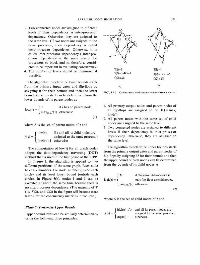
In Figure 3, the algorithm is applied to twodifferent partitions of the same graph. Each nodehas two numbers: the node number (inside eachcircle) and its level lower bound (outside eachcircle). In Figure 3(b), nodes and 5 can beexecuted at about the same time because there isno interprocessor dependency. (The meaning of T(1), T(2), and C(2) in the figure will become clearlater after the concurrency metric is introduced.)

Phase 2: Determine Upper Bounds

Upper bound levels can be similarly determined byusing the following three principles.

T(1)=8 T(1)=8T(2): 1+4+3: 8 T(2)= 1+3+1 5C(2) 8/8 C(2): 8/5

(a) (b)

FIGURE 3 Concurrency levelization and concurrency metric.

1. All primary output nodes and parent nodes ofall flip-flops are assigned to be M( maxtlow(t)).

2. All parent nodes with the same set of childnodes are assigned to the same level.

3. Two connected nodes are assigned to differentlevels if their dependency is inter-processordependency. Otherwise, they are assigned tothe same level.

The algorithm to determine upper bounds startsfrom the primary output gates and parent nodes offlip-flops by assigning M for their bounds and thenthe upper bound of each node can be determinedfrom the bounds of its child nodes as

M if has no child node or has

high(t) only flip-flops as child nodes,

minsesf(s) otherwise

where S is the set of child nodes of and

(2)

high(s) if s and all its parent nodes areassigned to the same processorf(s)

high(s)- otherwise


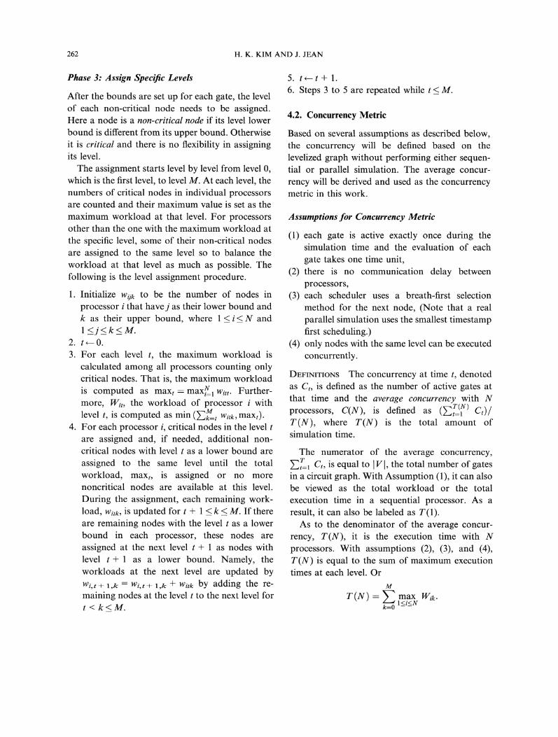
Phase 3: Assign Specific Levels

After the bounds are set up for each gate, the levelof each non-critical node needs to be assigned.Here a node is a non-critical node if its level lowerbound is different from its upper bound. Otherwiseit is critical and there is no flexibility in assigningits level.The assignment starts level by level from level 0,

which is the first level, to level M. At each level, thenumbers of critical nodes in individual processorsare counted and their maximum value is set as themaximum workload at that level. For processorsother than the one with the maximum workload atthe specific level, some of their non-critical nodesare assigned to the same level so to balance theworkload at that level as much as possible. Thefollowing is the level assignment procedure.

1. Initialize wijk to be the number of nodes inprocessor that have j as their lower bound andk as their upper bound, where _< i_< N and<_j<_k <_ M.

2. tO.3. For each level t, the maximum workload is

calculated among all processors counting onlycritical nodes. That is, the maximum workloadis computed as maxt- max/U__l witt. Further-more, Wit, the workload of processor withlevel t, is computed as min ()-]t:t witk, maxt).

4. For each processor i, critical nodes in the levelare assigned and, if needed, additional non-critical nodes with level as a lower bound are

assigned to the same level until the totalworkload, maxt, is assigned or no morenoncritical nodes are available at this level.During the assignment, each remaining work-load, Witk, is updated for + <_ k < M. If thereare remaining nodes with the level as a lowerbound in each processor, these nodes areassigned at the next level + as nodes withlevel + as a lower bound. Namely, theworkloads at the next level are updated byWi,t+ 1,k Wi,t+ 1,k -- Witk by adding the re-

maining nodes at the level to the next level fort<k<M.

5. tt+l.6. Steps 3 to 5 are repeated while < M.

4.2. Concurrency Metric

Based on several assumptions as described below,the concurrency will be defined based on thelevelized graph without performing either sequen-tial or parallel simulation. The average concur-rency will be derived and used as the concurrencymetric in this work.

Assumptions for Concurrency Metric

(1) each gate is active exactly once during thesimulation time and the evaluation of eachgate takes one time unit,

(2) there is no communication delay betweenprocessors,

(3) each scheduler uses a breath-first selectionmethod for the next node, (Note that a realparallel simulation uses the smallest timestampfirst scheduling.)

(4) only nodes with the same level can be executedconcurrently.

DEFINITIONS The concurrency at time t, denotedas Ct, is defined as the number of active gates atthat time and the average concurrency with N

[-T(N) Ct) /processors, C(N), is defined as

T(N), where T(N) is the total amount ofsimulation time.

The numerator of the average concurrency,

=l Ct, is equal to Vl, the total number of gatesin a circuit graph. With Assumption (1), it can alsobe viewed as the total workload or the totalexecution time in a sequential processor. As aresult, it can also be labeled as T(1).As to the denominator of the average concur-

rency, T(N), it is the execution time with Nprocessors. With assumptions (2), (3), and (4),T(N) is equal to the sum of maximum executiontimes at each level. Or

M

max Wik.r(g)I<i<N

k=O


where M is the maximum level in a levelizeddirected graph and Wik the number of level-knodes that are in processor such that < < N. (Ifwe consider graphs with weighted nodes, e.g., atask graph, Wik should be the sum of weights oflevel-k nodes in partition i.)

Therefore the concurrency metric C(N) can becomputed as

T(1) IWlC(N) T(N) t=0 max,<i<u Wik

Since VI- ’=0 E/N-- Wi, it can be shownmathematically that _< C(N)<_ N. If C(N)= N,which occurs when Wi is independent of i, thepartitioning is optimal from the point of con-currency. If C(N) 1, which occurs when-’]/N= Wik maxl<i<N Wik for all k, the partition-ing causes sequential processing even thoughmultiple processors are used.

In Figure 3, the levelization algorithm is appliedto two different partitions of the same graph. Ithappens that all the nodes are critical in eitherpartition and the node levels are indicated outsidethose nodes. For each partition, the concurrencymetric is computed and illustrated in the figure. Asshown in the figure, the partition in Figure 3(b)has higher concurrency metric value than the otherone. This result is consistent with the intuition andis as expected.

5. SIMULATION RESULTS ANDCOMPARISON

of that event. Even though the Time Warpalgorithm has a high degree of parallelism, thenumber of rollbacks must be reduced to get betterperformance.The experiments were performed on an Intel

Paragon XP/S machine and an IBM SP2 machine.The Paragon machine is a massively parallelprocessor that has a large number of computingnodes interconnected by a high-speed mesh net-work. Each node has two identical 50 MHz Intel i-860XP processors and 32 Mbytes of memory. Oneprocessor executes user and operating systemcodes while the other is dedicated to messagepassing. Each node runs the XP/S operationsystem using MPI communication environment.The IBM SP2 is also a massively parallel processorthat has a large number of computing nodesinterconnected by a high-speed multistage net-work. Each node of SP2 has a 75 MHz processorand 64 Mbytes of memory. Several of the largestsequential ISCAS benchmark circuits [2] were usedas test cases. Their characteristics are summarizedin Table I. One hundred random input vectorswere used for the simulation of each circuit and thefirst ten of them were used in the pre-simulation toget estimates of node activity levels and edgeweights. Note that in this section the pre-sirnulationis used only where it is explicitly specified. The gate-level unit delay model was adopted for thesimulations. For each of those ISCAS circuits,the CPP algorithm finished the partitioning part ofsimulation within 5 seconds on a sequential DECalpha 3000/400 workstation.

5.1. Simulation Model and Environment

In this paper, the effects of the CPP algorithm onthe Time Warp algorithm are studied. In the TimeWarp algorithm [8], a processor executes events ina timestamp order and the local simulation time ofa processor is called a local virtual time (LVT).Whenever a processor receives an event with atimestamp less than the LVT, it rolls backimmediately to the state just before the timestamp

TABLE ISCAS benchmark circuits

c6288 3376 32 32 0c7552 4951 206 108 0s9234 5808 36 39 211s13207.1 8651 62 152 638s15850.1 10383 77 150 534s38417 23843 28 106 1636s38584.1 20717 38 304 1426

No. of No. of No. of No. of No. ofCircuit gates input output flip-flops

gates gates


5.2. Performance Comparison

To facilitate comparison, three other partitioningalgorithms, including the random partitioning, thedepthfirst search (DFS) partitioning, and the stringpartitioning, were implemented and the MeTispackage that supported the multilevel partitioning[11] was used.

1. The random partitioning scheme randomlyassigns circuit gates into processors with theconstraint that each processor is allocatedroughly the same number of circuit gates. Eventhough the random partitioning scheme intro-duces a lot of communication overhead, it isexpected to provide pretty good load balancing[16, 24].

2. The DFS partitioning scheme uses a basicdepth first search to traverse a circuit graphstarting from a pseudo root that has onedirected edge to each primary input gate. Thetraversing is therefore guaranteed to visit eachgate once. The sequence of gates is thenassigned to the processors, with each processorgetting roughly equal number of gates [10, 15].This scheme generates partitions with relativelylow interprocessor communication andachieves balanced processor workloads. How-ever, the DFS scheme does not considerconcurrency issue, unlike the CPP algorithm.Note that both node activity levels and edgeweights were not considered in either randomor DFS scheme.

3. The string partitioning algorithm [17] is the firstalgorithm to consider concurrency and itproduces solutions of high degree of concur-rency. However it generates a lot of interpro-cessor communication because communicationbetween strings is not considered.

4. MeTis is a software package that implements amultilevel partitioning algorithm for irregulargraphs. It is known to produce high qualitysolutions for different applications, especially inreducing interprocessor communication [11].

The CPP algorithm was originally compared tothe random and the DFS algorithms on an Intel

Paragon machine. Because that machine wasphased out right before the development of theiCPP algorithm, the simulation results of the iCPPalgorithm, along with the string algorithm and theMeTis were from an IBM SP2 machine. That iswhy in this section not all algorithms arecompared together for parallel simulation results.When parallel simulations are not required for aperformance metric, such as the concurrencymetric, all those algorithms are compared at thesame time.The algorithms were evaluated by comparing

the following performance measures: concurrency,load balancing, the ratio of edge cut, the ratio ofexternal events, the ratio of erroneous events, theexecution time, and the speedup. Here the ratio ofedge cut is defined as the number of cut-edges (i.e.,edges between nodes on different processors)divided by the total number of edges in a circuit.The ratio of external events is defined as thenumber of external events divided by the totalnumber of external and internal events. These twoperformance measures are related to interproces-sor communication. Note that a cut-edge does notnecessarily produce an external event while anexternal event does imply the existence of a cut-edge.

Concurrency

The inherent parallelism of a circuit depends on itsstructure, such as the number of primary inputgates, the number of flip-flops, and the connectiv-ity of circuit gates. In general, a loosely connectedcircuit has high concurrency while a tightlyconnected circuit has relatively low concurrency.Table II summarizes the concurrency of severalcircuits after the application of those partitioningalgorithms. Figure 4 displays those results graphi-cally for the circuit s38417 with three partitioningalgorithms that produce a high degree of con-currency. It shows that the iCPP algorithmproduces better concurrency than MeTis doeswhile the string algorithm is the best in terms ofconcurrency.


TABLE II Concurrency metric

ExperimentCircuit Partitioning 2

No. of Processors5 10 16 20 32 40 52 64

String 2.0s38417 DFS 2.0

MeTis 2.0iCPP 1.9

s38584.1 iCPP 1.9s15850.1 iCPP 1.9

3.9 5.0 9.7 15.2 19.0 28.8 35.2 41.9 48.44.0 4.8 7.7 10.5 11.3 15.5 16.3 20.1 22.24.0 5.0 9.9 15.0 17.8 21.8 20.6 26.0 27.33.9 5.0 9.8 15.0 16.6 22.2 22.0 28.8 28.33.9 4.9 6.8 8.0 9.5 12.1 15.1 17.1 19.53.9 4.9 7.1 8.6 9.1 12.1 12.8 12.8 13.4

Concurrency50

45

40

35

30

25

20

15

10

Asyn + String + s38417Asyn + iCPP + s38417Asyn + Metis + s38417

0 8 16 24 32 40 48 56 64Number of Processors

FIGURE 4 Concurrency.

Ratio of Communication (percentage)100

90 RANDOM + s38584.1 -----/ String + s38584.1 --,--.80 j, DFS + s38584.170 CPP + s38584.1

iCPP + s38584.160

5O

4O

30

..-I0 ’ ’"’:

..-’0 ’-" *-: t: 7" "0 8 16 24 32 40 48 56 64

Number of Processors

FIGURE 5 Edge cut ratio.

Interprocessor Communication

In Figure 5, partitioning results of the s38584.1circuit are summarized in terms of the ratio of edgecut. As can be seen from the diagram, curves fordifferent partitioning algorithms exhibit the sametrend as the number of processors increases.Another observation is that the iCPP and theMeTis algorithms consistently produce lower ratioof edge cuts than those other four algorithms. As amatter of fact, when bi-partitioning (two-proces-sor partitioning) is performed, the ratio of externalevents for the iCPP algorithm is 1.5%. Thiscompares favorably with several other partitioningalgorithms such as Flip-flop-Clustering (10%),Min-Cut (15%), and Levelizing (20%). These

results were reported in [26]. Even though theCorolla-clustering algorithm [26] with its 0.6%ratio of external events for bi-partitioning defi-nitely outperforms the iCPP algorithm in thisregard, it is relatively slow and does not takeconcurrency into consideration. The figure alsoshows that the ratio of edge cuts with the iCPPalgorithm is only 12.5% even when 64 processorsare used. It is therefore interesting to check out theother limiting factor in Time Warp simulation, i.e.,the rollback overhead.

Event Rollback

The ratios of erroneous events versus the numberof processors are summarized in Figure 6 for the


Ratio of Erroneous Events (percentage)50

4O

3O

2O

10

,l,

0 8 16 24 32 40 48 56 64Number of Processors

FIGURE 6 Ratio of erroneous events.

Execution Time (in seconds)

ii

0

0

0

RANDOM + s38584.1DFS + s38584.1CPP + s38584.1

90 iki"\60

\ "-,. ",..30 ,,. "..,. .....

=================================0 8 16 24 32 40 48 56 64


FIGURE 7 Execution time.

three partitioning schemes. The circuit is thes38584.1 circuit that has 20717 gates. To read thediagram, see for example, less than 18 percent ofevents were canceled when the CPP algorithm wasused for 64 processors. Apparently the CPPalgorithm introduces lower ratios of erroneousevents than those of the DFS and the RANDOMschemes.

Simulation Execution Time

Figure 7 shows the execution times for simulatingthe s38584.1 circuit with different algorithms. Herethe execution time excludes the time for partition-ing, reading input vectors, and printing outputvectors. Note that, when the number of processorsis fixed, experiments show that the execution timeincreases linearly with the number of randomlygenerated input vectors. For real circuit simula-tions, the circuit is expected to be larger and muchhigher number of input vectors are required. Ittherefore makes sense to exclude the time toperform partitioning since it is performed onlyonce as an initialization step.

Table III lists the values used in Figure 7 as wellas the execution times for simulating two othercircuits. It shows that the parallel simulation ofs38584.1 can be executed in 5 seconds using 64processors (with node activities and edge weightsobtained through pre-simulation) while the se-quential simulation takes 140seconds. It alsoshows that, when the same number of processorsis used, the parallel simulation with the CPPalgorithm is usually faster than with the other twoalgorithms for the s38584.1 circuit. In particular,when two processors are used, the RANDOM andDFS algorithms do not get any speedup becausethe RANDOM algorithm suffers from a lot ofinterprocessor communication while the DFSalgorithm does not provide a high degree of loadbalancing over time, i.e., it does not provideenough concurrency and therefore causes a lot ofrollbacks.Note that the pre-simulation speeds up parallel

simulations in two ways. Edge weights represent-ing event frequencies over edges can be used toreduce the interprocessor communication and thenode activity level representing event frequencies


TABLE III The execution time (in seconds); CPP (= CPP without node activity), Cp3(-- CPP with pre-simulation)

Experiment No. of ProcessorsCircuit Partitioning 2 4 8 16 24 32 40 48 56 64

RAN DOM 141.0 209.9 118.0 68.2 38.8 26.1 22.9 19.1 16.1 15.4 12.0s38584.1 DFS 141.0 148.4 77.0 49.8 22.9 17.9 12.8 10.8 9.2 8.1 7.5

CPP 141.0 117.9 55.9 27.6 14.5 10.7 9.4 10.9 9.5 7.6 6.6CP 141.0 99.2 49.1 25.5 13.8 9.7 7.9 6.8 6.4 5.3 5.0

s38417 CP 103.0 67.9 32.4 15.2 8.2 6.3 4.8 4.7 4.2 3.2 3.3s15850.1 CP 42.5 28.4 14.1 8.3 5.8 5.0 4.3 4.0 3.9 3.2 3.4

inside a node can be used to get better loadbalancing.

Load Balancing

Figure 8 shows the processor workloads obtainedwith parallel simulations when the CPP algorithmis used with or without the pre-simulation. Eachpoint in the figure denotes the total number ofevents evaluated for a specific processor. Appar-ently better load balancing is achieved when thenode activity levels and edge weights are availablein Phase 3 of the CPP algorithm. Note thatunbalanced workload increases the number oferroneous events, increases the amount of roll-backs, and prolongs a parallel simulal:ion.

Processor Workload (No. of events evaluated)120000

100000

80000

60000

40000

20000

NO NODE ACTIVITY + CPP + s38584.1NODE ACTIVITY + CPP + s38584.1

8 16 24Processor Number

32

Speedup

Speedup is defined as the ratio of the executiontime of the best sequential simulator to that of theparallel simulator. For most circuits, reasonablespeedups may be obtained when the number ofprocessors is small and there are enough events tobe executed concurrently. In Figure 9, speedupsobtained with different algorithms are shown. Thefigure shows that the performance of a Time Warpsimulation is very sensitive to partitioning whenlarge number of processors are employed and theCPP algorithm achieves better speedup than thoseof the RANDOM and the DFS partitioningalgorithms. Note that when the number ofprocessors is near 40, the CPP algorithm withoutpre-simulation degrades and performs roughly the

Speedup35

30

25

20

15

10

" CPP+s38584.1’--,- "DFS + s38584.1 --.-

RANDOM + s38584.1

""0 8 16 24 32 40 48 56 64


FIGURE 8 Processor workload with 32 processors. FIGURE 9 Speedups without pre-simulation.


same as DFS does. By comparing this phenomen-on to the 538584.1 curve in Figure 10 where thespeedups of three large ISCAS89 circuits aredisplayed for the CPP with pre-simulation, an-other observation is that, when the number ofprocessors is below 32, the performance of theCPP algorithm is almost not influenced by thedecision to consider node activity levels and edgeweights. However, when more processors areadded, the advantage of having extra knowledgefrom the pre-simulation becomes critical. Also canbe observed from Figure 10 is that a significantspeedup of 31 with 64 processors was obtained forthe s38417 circuit.

Performance on the IBM SP2

Among the algorithms considered, three of themthat are more competitive are tested on an IBMSP2 machine. These include the proposed iCPPalgorithm, the string algorithm, and the MeTis. Allsimulations are performed with 1000 input vectorsusing the Time Warp parallel simulation modeland is globally synchronized every 100 inputvectors. Figure 11 shows the resulting speedups

Speedup35

3O

25

2O

15

10

ACTIVITY + CPP- s384 7’ --,----ACTIVITY + CPP + s38584.1ACTIVITY + CPP + s15850.1 /

// .-’"

..A ./"

/// //’"

,,//’" ...//,/..............’"

0 8 6 24 a2 40 48 56 64Number of Processors

FIGURE 10 Speedups with pre-simulation for differentcircuits.

25SpeedupMeTis+s38417iCPP + s38417String + s38417

20

15

10

8 16 24 32Number of Processors

FIGURE 11 Speedups on the IBM SP2 wihout pre-simula-tion.

for the s38417 circuit without pre-simulation.Among those three partitioning algorithms, thestring algorithm is the slowest one while the MeTisoutperforms the iCPP algorithm with only twoexceptions (when there are 8 processors and 32processors, respectively). Recall that in Figure 4, interms of concurrency, the string algorithm per-forms the best and the MeTis is the worst one. Itseems that the amount of interprocessor commu-nication for the iCPP algorithm still needs to beminimized. An analysis of the results shows thatthe iCPP produces much more rollbacks than theMeTis does. Therefore for the iCPP algorithm tobe more competitive, there is a need to reduce therollback ratio which may be achieved by resyn-chronizing the simulation more frequently. This inturn requires a more efficient algorithm for theGVT (global virtual time) computation.

6. CONCLUSIONS

In this study, the effect of concurrency, orinstantaneous load balancing, is considered in the


development of a partitioning algorithm forparallel logic simulation. The resulting algorithmis called the improved concurrency preservingpartitioning (iCPP) algorithm. The algorithm hasthree phases so that three different goals can beseparately considered in order to achieve a goodcompromise. Unlike most other partitioning algo-rithms, the iCPP algorithm preserves the concur-rency of a circuit by dividing the entire circuit intosubcircuits according to the distribution of primaryinputs and flip-flops. Preserving concurrency pro-duces better instantaneous load balancing andreduces the gap between local virtual times (LVTs).It in turn reduces the number of erroneous events.Therefore with a good compromise among threeconflicting goals, the iCPP algorithm producesreasonably good performance for large circuits.To measure the concurrency, a concurrency

metric that requires neither sequential nor parallelsimulation is developed and used to compare sixdifferent algorithms, including the random, thedepth-first-search (DFS), the string, the MeTis,the CPP, and the iCPP. The results indicate thatthe iCPP algorithm preserves concurrency prettywell while at the same time it achieves lower inter-processor communication compared to the stringalgorithm (which also targets concurrency expli-citly). In addition to using the concurrency metric,optimistic discrete event simulations are per-formed on an Intel Paragon and an IBM SP2 tocompare the effects of different partitioning algo-rithms on parallel logic simulations. The largescale comparison effort by itself represents a prettyunique contribution to the research community ofparallel logic simulation.

Acknowledgements

This research is supported by an Ohio State Boardof Regent Research Investment grant. The authorswould like to thank the ASC Major SharedResource Center of the US Air Force for provid-ing Paragon access and Argonne National La-boratory and Ohio Supercomputer Center forallowing the use of their IBM SP2 machines.

References

[1] Bailey, M. L., Briner, J. V. Jr. and Chamberlain, R. D.(1994). "Parallel Logic Simulation of VLSI Systems",ACM Computing Surveys, 26(3), 255-294.

[2] Brglez, F., Bryan, D. and Kozminski, K. (1989)."Combinational Profiles of Sequential Benchmark Cir-cuits", Proc. of the IEEE International Symp. on Circuitsand Systems, pp. 1929-1934.

[3] Boukerche, A. and Tropper, C. (1994). "A StaticPartitioning and Mapping Algorithm for ConservativeParallel Simulations", Proc. of 8th Workshop on Paralleland Distributed Simulation, pp. 164-172.

[4] Boukerche, A. and Tropper, C. (1995). "SGTNE: Semi-Global Time of the Next Event Algorithm," Proc. of 9thWorkshop on Parallel and Distributed Simulation,pp. 68- 77.

[5] Briner, J. V. Jr. (1990). "Parallel Mixed-Level Simulationof Digital Circuits Using Virtual Time," Ph.D. Disserta-tion, Duke University.

[6] Chamberlain Roger, D. and Henderson Cheryl, D. (1994)."Evaluating the Use of Pre-Simtilation in VLSI CircuitPartitioning," Proc. of 8th Workshop on Parallel andDistributed Simulation, pp. 139-146.

[7] Fiduccia, C. M. and Mattheyses, R. M. (1982). "A Linear-Time Heuristic for Improving Network Partitions,"Proc. of the Design Automation Conference, pp. 175-181.

[8] Jefferson, D. R. (1985). "Virtual Time," ACM Trans. onProgramming Languages and Systems, 7(3), 404-425.

[9] Vikas Jha and Rajive Bagrodia (1996). "A PerformanceEvaluation Methodology for Parallel Simulation Proto-cols," Proc. of lOth Workshop on Parallel and DistributedSimulation, pp. 180-185.

[10] Kapp, K. L., Hartrum, T. C. and Wailes, T. S. (1995)."An Improved Cost Function for Static Partitioning ofParallel Circuit Simulations Using a Conservative Syn-chronization Protocol," Proc. of9th Workshop on Paralleland Distributed Simulation, pp. 78- 85.

[11] Karypis, G. and Kumar, V. (1995). "Multilevel graphpartition and sparse matrix ordering," Int’l Conf onParallel Processing, 3, 113 122.

[12] Keller, J., Rauber, T. and Rederlechner, B. (1996)."Conservative Circuit Simulation on Shared-MemoryMultiprocessors," Proc. of lOth Workshop on Paralleland Distributed Simulation, pp. 126-134.

[13] Kernighan, B. W. and Lin, S. (1970). "An EfficientHeuristic Procedure for Partitioning Graphs," Bell SystemTechnical Journal, 49, pp. 291 307.

[14] Hong, K., Kim and Jack, Jean (1996). "ConcurrencyPreserving Partitioning (CPP) for Parallel Logic Simula-tion," Proc. of lOth Workshop on Parallel and DistributedSimulation, pp. 98-105.

[15] Pavlos, Konas and Pen-Chung, Yew (1991). "ParallelDiscrete Event Simulation on Shared-Memory Multi-processors," The 24th Annual Simulation Symposium,pp. 134- 148.

[16] Kravitz, S. A. and Ackland, B. D. (1988). "Static vs.Dynamic Partitioning of Circuits for a MOS TimingSimulator on A Message-Based Multiprocessor," Proe. ofthe SCS Multiconference on Distributed Simulation,pp. 136- 140.

[17] Levendel, V. H., Menon, P. R. and Patel, S. H. (1982)."Special Purpose Computer for Logic Simulation UsingDistributed Processing," Bell System Technical Journal,61(10), 2873-2909.


[18] Yi-Bing, Lin (1992). "Parallelism analyzers for paralleldiscrete event simulation," ACM Transactions on Model-ing and Computer Simulation, pp. 239-264.

[19] Malloy, B. A., Lloyd, E. L. and Sofia, M. L. (1994)."Scheduling DAG’s for Asynchronous MultiprocessorExecution," IEEE Transactions on Parallel and DistributedSystems, 5(5), 495- 508.

[20] Manjikian, N. and Loucks, W. M. (1993). "HighPerformance Parallel Logic Simulation on a Network ofWorkstations," Proc. of 7th Workshop on Parallel andDistributed Simulation, pp. 76-84.

[21] Mueller-Thuns, R. B., Saab, D. G., Damiano, R. F. andAbraham, J. A. (1993). "VLSI Logic and Fault Simulationon General-Purpose Parallel Computers," IEEE Trans. onComputer-Aided Design, 12(3), 446-460.

[22] Biswajit Nandy and Loucks, W. M. (1992). "An Algo-rithm for Partitioning and Mapping Conservative ParallelSimulation onto Multicomputers," Proc. of6th Workshopon Parallel and Distributed Simulation, pp. 139- 146.

[23] Laura, A., Sanchis (1989). "Multiple-Way NetworkPartitioning," IEEE Transactions on Computers, 38(1),62-81.

[24] Smith, S. P., Underwood, B. and Mercer, M. R. (1987)."An Analysis of Several Approaches to Circuit Partition-ing for Parallel Logic Simulation," IEEE InternationalConference on Computer Design, pp. 664-667.

[25] Soule, L. and Gupta, A. (1989). "Characterization ofParallelism and Deadlocks in Distributed Digital LogicSimulation," Proc. of the 26th Design Automation Conf.,pp. 81-86.

[26] Sporrer, C. and Bauer, H. (1993). "Corolla Partitioningfor Distributed Logic Simulation of VLSI-Circuits," Proc.of 7th Workshop on Parallel and Distributed Simulation,pp. 85- 92.

Authors’ Biographies

Hong K. Kim is currently working towards thePh.D degree in computer science at Wright StateUniversity, Dayton, Ohio. He received the M.S.degree in computer science and the B.S. degree inindustrial engineering from New Jersey Institute ofTechnology, Newark, N.J., and Korea University,Korea, respectively. His research interests includeparallel simulation, partitioning algorithms, com-puter aided design of circuits, and distributedcomputing. He is a member of ACM and SCS.

Jack Shiann-Ning Jean received the B.S. andM.S. degrees from the National Taiwan University,Taiwan, in 1981 and 1983, respectively, and thePh.D. degree from the University of SouthernCalifornia, Los Angeles, C.A., in 1988, all in elec-trical engineering. In 1989, he received a researchinitiation award from the National Science Foun-dation. Currently he is an Associate Professor in theComputer Science and Engineering DePartment ofWright State University, Dayton, Ohio. Hisresearch interests include parallel processing,reconfigurable computing, and machine learning.

International Journal of

AerospaceEngineeringHindawi Publishing Corporationhttp://www.hindawi.com Volume 2010

RoboticsJournal of

Hindawi Publishing Corporationhttp://www.hindawi.com Volume 2014


Active and Passive Electronic Components

Control Scienceand Engineering

Journal of



RotatingMachinery


Hindawi Publishing Corporation http://www.hindawi.com

Journal ofEngineeringVolume 2014

Submit your manuscripts athttp://www.hindawi.com

VLSI Design



Shock and Vibration


Civil EngineeringAdvances in

Acoustics and VibrationAdvances in



Electrical and Computer Engineering

Journal of

Advances inOptoElectronics

Hindawi Publishing Corporation http://www.hindawi.com

Volume 2014

The Scientific World JournalHindawi Publishing Corporation http://www.hindawi.com Volume 2014

SensorsJournal of


Modelling & Simulation in EngineeringHindawi Publishing Corporation http://www.hindawi.com Volume 2014


Chemical EngineeringInternational Journal of Antennas and

Propagation




Navigation and Observation



DistributedSensor Networks


Concurrency Preserving Partitioning Algorithm...

Documents

Transcript of Concurrency Preserving Partitioning Algorithm...