ARGONNE NATIONAL LABORATORY

9700 South Cass Avenue

Argonne, Illinois 60439

Concrete Structure Design Using Mixed-Integer NonlinearProgramming with Complementarity Constraints

Andres Guerra, Alexandra M. Newman, and Sven Leyffer

Mathematics and Computer Science Division

Preprint ANL/MCS-P1869-1109

November 24, 2009

This work was supported by the Office of Advanced Scientific Computing Research, Office of Science, U.S. Department of

Energy, under Contract DE-AC02-06CH11357.

Contents

1 Introduction and Literature Review 1

2 Problem Description and Formulation 4

2.1 Parameters and Constants . . . . . . . . . . . . . . . . . . . . . . . . . . . . . . . . . . . . . . 4

2.2 Variables . . . . . . . . . . . . . . . . . . . . . . . . . . . . . . . . . . . . . . . . . . . . . . . 4

2.3 Objective and Constraints . . . . . . . . . . . . . . . . . . . . . . . . . . . . . . . . . . . . . . 4

2.4 Problem Discussion . . . . . . . . . . . . . . . . . . . . . . . . . . . . . . . . . . . . . . . . . . 12

3 Model Instances 16

3.1 Parameter Values . . . . . . . . . . . . . . . . . . . . . . . . . . . . . . . . . . . . . . . . . . . 16

3.2 Initialization of Variables . . . . . . . . . . . . . . . . . . . . . . . . . . . . . . . . . . . . . . 17

3.3 Problem Size and Structure . . . . . . . . . . . . . . . . . . . . . . . . . . . . . . . . . . . . . 18

3.4 Choice of MINLP Algorithm . . . . . . . . . . . . . . . . . . . . . . . . . . . . . . . . . . . . 18

4 Numerical Results 19

4.1 Algorithm Performance . . . . . . . . . . . . . . . . . . . . . . . . . . . . . . . . . . . . . . . 19

4.2 Objective Function Values . . . . . . . . . . . . . . . . . . . . . . . . . . . . . . . . . . . . . . 20

4.3 Solution Characteristics . . . . . . . . . . . . . . . . . . . . . . . . . . . . . . . . . . . . . . . 22

5 Conclusions 24

A Convex Hull Reformulation 25

Concrete Structure Design Using Mixed-Integer NonlinearProgramming with Complementarity Constraints

Andres Guerra† • Alexandra M. Newman‡ • Sven Leyffer∗

†Division of Engineering, Colorado School of Mines, Golden, CO 80401

‡Division of Economics and Business, Colorado School of Mines, Golden, CO 80401∗Mathematics and Computer Science Division, Argonne National Laboratory, Argonne, IL 60439

aguerra@mines.edu • newman@mines.edu • leyffer@mcs.anl.gov

November 24, 2009

Keywords: complementarity problems, applications in optimization, mixed integer programming

Abstract

We present a mixed-integer nonlinear programming (MINLP) formulation to achieve minimum-costdesigns for reinforced concrete (RC) structures that satisfy building code requirements. The objectivefunction includes material and labor costs for concrete, steel reinforcing bars, and formwork according totypical contractor methods. Restrictions enforce correct geometry of the cross-section dimensions for eachelement and relative sizes of cross-section dimensions of elements within the structure. Other restrictionsdefine a stiffness and displacement correlation among all structural elements via finite element analysis.

The design of minimum cost RC structures introduces a new class of optimization problems, namely,mixed-integer nonlinear programs with complementarity constraints. The complementarity constraintsare used to model RC element strength and ACI code-required safety factors. We reformulate thecomplementarity constraints as nonlinear equations and show that the resulting ill-conditioned MINLPscan be solved by using an off-the-shelf MINLP solver. Our work provides discrete-valued design solutionsfor an explicit representation of a process most often performed implicitly with iterative calculations.

We demonstrate the capabilities of a mixed-integer nonlinear algorithm, MINLPBB, to find optimalsizing and reinforcing for cast-in-place beam and column elements in multistory RC structures. Probleminstances contain up to 678 variables, of which 214 are integer, and 844 constraints, of which 582 arenonlinear. We solve problems to local optimality within a reasonable amount of computational time, andwe find an average cost savings over typical-practice design solutions of 13 percent.

1 Introduction and Literature Review

Reinforced concrete (RC) is commonly used to build cost-efficient and durable structures. Important prop-

erties of RC are (1) significant compressive strength that increases over time, (2) low maintenance, (3) fire

resistance, and (4) constitution of inexpensive local materials such as sand, gravel, and water. RC consists

of large portions of sand and gravel and smaller portions of cement and steel reinforcing bars. The cement

and water chemically interact to cohere the sand and gravel into a solid mass surrounding the reinforcing

bars. Cast-in-place RC construction refers to methods used to fabricate structural elements in the intended

design position and location. Wet concrete is placed into a wooden or steel formwork that holds the concrete

in place until it develops sufficient self supporting strength. Reinforcement is placed within the formwork

before pouring the concrete so that the concrete hardens around the reinforcement. The combination of

concrete and reinforcing bars provides elements that can withstand large forces. The design of RC involves

1

selecting dimensions consisting of discrete-valued element width and depth, reinforcing bar sizes, and the

number of bars ensuring structural integrity. The goal of this paper is to provide a sound mathematical

model and solution methodology that yield minimum cost designs of large and complex RC buildings.

The analysis procedures for RC that are typically adopted in practice assume a structural system with

a fixed initial stiffness. The demand on the RC elements in terms of displacements and forces depends on

the applied loads and relative stiffness of elements, where stiffness is a measure of displacement with respect

to force. A fixed initial stiffness distribution is necessary to calculate the demand, or internal forces, in a

statically indeterminate structure. Engineers then design element dimensions to resist these internal forces,

which, unfortunately, are inconsistent with the internal forces associated with the final design dimensions.

This inconsistency creates unnecessarily expensive and overengineered solutions.

An explicit formulation of the RC design problem improves the fidelity of the current-practice structural

analysis by resolving inconsistencies between the initial design assumptions and the final design dimensions.

We develop an explicit formulation for the RC design problem using continuous and continuously differ-

entiable expressions to enforce relationships between decision variables. We represent Boolean expressions

with binary variables whose continuous relaxations yield differentiable expressions. An explicit formulation

provides a feasible solution directly and completely computed without an iterative procedure, and in our

case, locally optimal solutions that can be easily evaluated. An explicit formulation also allows for the use

of a robust solver on larger problems that produce better-quality solutions in less computation time.

In our explicit mixed-integer nonlinear optimization model, we use integer variables to represent the width

and depth of each element and the number of reinforcing bars. We employ binary variables to select discrete

reinforcing bar sizes from a set of potential sizes and to represent discrete decisions for formwork reuse.

Continuous decision variables relate to applied forces and resistive capacity of each element. Formulating

the problem with integer variables allows for an objective function including material and labor costs for

concrete, steel reinforcing bars, and formwork in accordance with typical methods used by contractors.

Constraints or restrictions enforce (1) the correct geometry of the cross-section dimensions for each element,

(2) the relative sizes of cross-section dimensions of elements within the structure, (3) finite-element analysis

equilibrium equations that define the appropriate relationships between forces, displacements, and stiffness,

(4) the resistive capacities of each element, (5) bounds on the applied loads relative to the resistive capacities

of each element, and (6) upper and lower bounds on the variables.

Our model provides an example of a new class of challenging optimization problems, namely mixed-integer

nonlinear optimization problems with complementarity constraints. The complementarity constraints are

necessary to model the resistive forces provided by the concrete, elastic-perfectly plastic material response

for the steel reinforcement. We use American Concrete Institute (ACI) code requirements to include the

appropriate safety factors and minimum axial load requirements for flexural elements. We reformulate the

complementarity constraints as nonlinear inequalities. This approach gives rise to a degenerate MINLP that

violates the Mangasarian-Fromowitz constraint qualification at any feasible point; see, for example, Scheel

and Scholtes (2000). We show that the resulting MINLP can nonetheless be solved reliably using a suitable

off-the-shelf MINLP solver. We demonstrate the capability of our explicit formulation to find lower-cost and

more efficient solutions than currently found in practice, extending RC design optimization.

The use of optimization in RC design is not new. The first instances of optimization techniques for RC

structures were explicit methods to determine inelastic solutions with fixed element dimensions. Inelastic

material behavior incorporates material nonlinearities, whereas elastic material behavior contains linear

material properties. De Donato and Maier (1972) were among the first to minimize a quadratic function

subject only to sign constraints, incorporating inelastic material behavior for RC structural analysis. Prior

to the problem posed by De Donato and Maier, an inelastic solution of an RC structure with fixed element

2

dimensions was difficult to obtain, especially for statically indeterminate problems that require discretization

into finite-elements in order to accurately capture structural behavior (most real-world problems require

discretization). A study by Corradi et al. (1974) formulates and solves a linear complementarity problem

by overrelaxation to find inelastic solutions for multistory frames discretized into finite elements with fixed

element dimensions. Kaneko (1977), Maier et al. (1982), and Dinno and Mekha (1995) expand the use

of complementarity to perform inelastic analysis of RC structures with fixed element dimensions. When

the element dimensions are fixed, finite element methods model constitutive behavior using mathematical

operations on linear systems of equations. When element dimensions are variables, finite element analysis

becomes increasingly difficult because the system of equations contains nonlinear functions of the element

dimensions. We further discuss finite element methods for frames in Section 2.3.1.

While the methods previously discussed use mathematical programming techniques to model inelastic

behavior for structures with fixed element dimensions, Krishnamoorthy and Mosi (1981) and Dinno and

Mekha (1993) include element dimensions as design variables and search for minimum cost solutions in

addition to using complementarity constraints to define inelastic behavior of RC frames. However, to find

solutions for reasonably sized buildings, Krishnamoorthy and Mosi (1981) include variables to describe

the reinforcing bar areas and determine the width and depth of elements a priori. Dinno and Mekha

(1993) include variables to describe the width and depth of elements and to determine the reinforcing bar

areas a priori. The objective functions in these studies include simplified costs for concrete, formwork, and

reinforcement that do not entirely capture construction practices. Both papers enforce structural stability

by ensuring that resistive forces are greater than applied forces, which are determined by finite element

analysis. Reducing the number of design variables facilitates solving problems with a larger number of story

levels but requires implicit, or iterative, methods to find a feasible solution because the number and size of

reinforcing bars depend on the width and height of each structural element.

Ferris and Tin-Loi (1999) present an explicit formulation to find minimum-weight solutions for trusslike

structures with complementarity constraints that incorporate inelastic behavior. We consider structures with

a greater number of degrees of freedom than trusslike structures have. However, this work demonstrates the

use of complementarity constraints in explicit structural optimization problems. Horowitz and Moraes (2005)

utilize MINLPBB to solve a problem with complementarity constraints to determine failure loads (rather

than actual dimensions) of a continuous RC beam with inelastic material properties. Horowitz and Moraes

demonstrate the ability to conduct complex inelastic analysis of RC structures using explicit methods.

Much of the remaining work in optimal design of RC structures excludes complementarity constraints

and evaluates structural behavior with elastic material properties to find solutions for buildings with a

larger number of design variables. Models using elastic (rather than inelastic) material properties generally

preclude the need for complementarity constraints. Fadaee and Grierson (1996), Balling and Yao (1997),

and Balling (2002) develop multistep approaches in conjunction with NLP techniques to find minimum-cost

solutions with elastic material properties. Fadaee and Grierson (1996) develop implicit methods for three-

dimensional RC frames with fewer than 25 continuous-valued variables. Balling and Yao (1997) and Balling

(2002) use postprocess rounding operations to obtain discrete-valued, constructible design solutions for two-

dimensional RC frames. To find solutions for problems with a larger number of story levels, Balling and

Yao (1997) reduce the number of variables that require rounding. However, their simplifying assumptions

diminish solution quality. More recently, Guerra and Kiousis (2006) use sequential quadratic programming to

determine optimal design solutions of two-dimensional RC structures. They implement a rounding heuristic

that requires the solution of a secondary optimization problem in which many of the decision variable values

are fixed based on the solution of the monolith. Guerra and Kiousis find solutions for problems with a similar

number of story levels as those demonstrated by Balling and Yao (1997) without simplifying assumptions

3

that reduce solution quality. The objective function presented by Guerra and Kiousis advances previous

studies by including changing unit costs as a function of the decision variables to more accurately incorporate

construction practices. Lee and Ahn (2003) and Camp et al. (2003) implement genetic algorithms that search

for discrete-valued solutions of beam and column elements in RC frames. Like many others, the authors

implement elastic material properties. The search for discrete-valued solutions using genetic algorithms is

difficult because of the nonlinearities in the model, as well as the large number of combinations of possible

element dimensions.

The remainder of this paper is organized such that in Section 2 we present the problem description and

formulation and in subsequent sections we present numerical results.

2 Problem Description and Formulation

We begin by describing the model in general terms, then present and justify the mathematical formulation,

and finally describe the formulation in detail.

2.1 Parameters and Constants

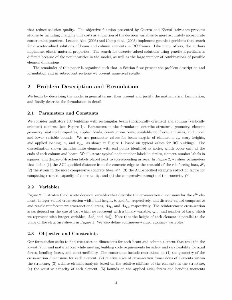
We consider multistory RC buildings with rectangular beam (horizontally oriented) and column (vertically

oriented) elements (see Figure 1). Parameters in the formulation describe structural geometry, element

geometry, material properties, applied loads, construction costs, available reinforcement sizes, and upper

and lower variable bounds. We use parameter values for beam lengths of element e, le, story heights,

and applied loading, ue and vψje, as shown in Figure 1, based on typical values for RC buildings. The

discretization shown includes finite elements with end points identified as nodes, which occur only at the

ends of each column and beam. We illustrate typical node number labels in circles, element number labels in

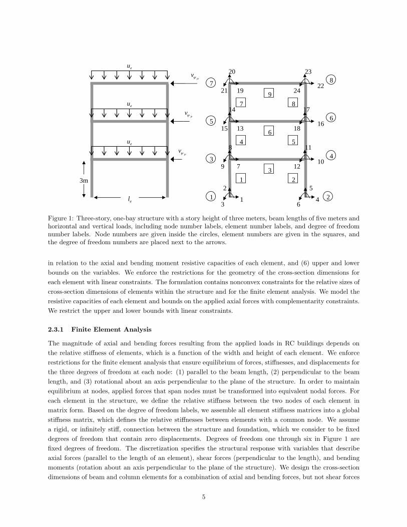
squares, and degree-of-freedom labels placed next to corresponding arrows. In Figure 2, we show parameters

that define (1) the ACI-specified distance from the concrete edge to the centroid of the reinforcing bars, dp,

(2) the strain in the most compressive concrete fiber, ǫcu, (3) the ACI-specified strength reduction factor for

computing resistive capacity of concrete, β1, and (4) the compressive strength of the concrete, fc′.

2.2 Variables

Figure 2 illustrates the discrete decision variables that describe the cross-section dimensions for the eth ele-

ment: integer-valued cross-section width and height, be and he, respectively, and discrete-valued compressive

and tensile reinforcement cross-sectional areas, As1e and As2e, respectively. The reinforcement cross-section

areas depend on the size of bar, which we represent with a binary variable, yem, and number of bars, which

we represent with integer variables, As#1e and As#2e. Note that the height of each element is parallel to the

plane of the structure shown in Figure 1. We also define continuous-valued auxiliary variables.

2.3 Objective and Constraints

Our formulation seeks to find cross-section dimensions for each beam and column element that result in the

lowest labor and material cost while meeting building code requirements for safety and serviceability for axial

forces, bending forces, and constructibility. The constraints include restrictions on (1) the geometry of the

cross-section dimensions for each element, (2) relative sizes of cross-section dimensions of elements within

the structure, (3) a finite element analysis based on the relative stiffness of the elements in the structure,

(4) the resistive capacity of each element, (5) bounds on the applied axial forces and bending moments

4

31

2

8

9 7

4

5

6

10

11

12

43

1 2

1 2

3

14

15 1316

17

18

65

4 5

6

20

21 1922

23

24

87

7 8

9

jev\

jev\

jev\

eu

eu

eu

el

3m

Figure 1: Three-story, one-bay structure with a story height of three meters, beam lengths of five meters andhorizontal and vertical loads, including node number labels, element number labels, and degree of freedomnumber labels. Node numbers are given inside the circles, element numbers are given in the squares, andthe degree of freedom numbers are placed next to the arrows.

in relation to the axial and bending moment resistive capacities of each element, and (6) upper and lower

bounds on the variables. We enforce the restrictions for the geometry of the cross-section dimensions for

each element with linear constraints. The formulation contains nonconvex constraints for the relative sizes of

cross-section dimensions of elements within the structure and for the finite element analysis. We model the

resistive capacities of each element and bounds on the applied axial forces with complementarity constraints.

We restrict the upper and lower bounds with linear constraints.

2.3.1 Finite Element Analysis

The magnitude of axial and bending forces resulting from the applied loads in RC buildings depends on

the relative stiffness of elements, which is a function of the width and height of each element. We enforce

restrictions for the finite element analysis that ensure equilibrium of forces, stiffnesses, and displacements for

the three degrees of freedom at each node: (1) parallel to the beam length, (2) perpendicular to the beam

length, and (3) rotational about an axis perpendicular to the plane of the structure. In order to maintain

equilibrium at nodes, applied forces that span nodes must be transformed into equivalent nodal forces. For

each element in the structure, we define the relative stiffness between the two nodes of each element in

matrix form. Based on the degree of freedom labels, we assemble all element stiffness matrices into a global

stiffness matrix, which defines the relative stiffnesses between elements with a common node. We assume

a rigid, or infinitely stiff, connection between the structure and foundation, which we consider to be fixed

degrees of freedom that contain zero displacements. Degrees of freedom one through six in Figure 1 are

fixed degrees of freedom. The discretization specifies the structural response with variables that describe

axial forces (parallel to the length of an element), shear forces (perpendicular to the length), and bending

moments (rotation about an axis perpendicular to the plane of the structure). We design the cross-section

dimensions of beam and column elements for a combination of axial and bending forces, but not shear forces

5

because the influence of shear forces is not significant in long, slender elements (Inel and Ozmen, 2006). In

the formulation we show all constraints for the finite element analysis but provide only that the relative

stiffnesses between elements are functions of the element dimensions. The specific equations for the relative

stiffnesses of elements are given in Guerra (2008).

2.3.2 Resistive Capacity of Reinforced Concrete

The capacity to resist applied forces, or resistive capacity, of an RC element is a function of the element

width and height as well as the reinforcement areas and strain. Recall that the magnitude of applied forces

is also a function of the element width and height. Strain is a unitless variable that describes the change

of length relative to the effective length over which the displacements occur. Axial and bending forces in

RC buildings result in cross-sections that experience both elongating and shortening strains. We enforce

restrictions to develop a linear strain distribution as shown in Figure 2 using variables that describe the

location of the neutral axis, ce, and strain at the location of the compressive and tensile reinforcement, ǫseand ǫte, respectively. The neutral axis defines the location of zero strain. Figure 2 illustrates one instance of a

linear strain distribution in which compressive strain above the location of the neutral axis is associated with

shortening and tensile strain below the neutral axis is associated with elongation. Concrete provides large

resistance for compressive strains but cracks when elongated and provides no resistance to tensile strains.

Compressive reinforcement resists forces associated with shortening an element, and tensile reinforcement

predominately resists forces associated with elongating an element. Tensile reinforcement sometimes provides

compressive resistance when the location of the neutral axis is below the location of the tensile reinforcement.

The resistive forces provided by the concrete, compressive reinforcement, and tensile reinforcement are a

function of the location of the neutral axis, the strain in the compressive reinforcement, ǫse, and strain in the

tensile reinforcement, ǫte, respectively. Figure 2 illustrates the resistive forces of the concrete, compressive

reinforcement, and tensile reinforcement in relation to the linear strain distribution. The concrete resistive

force is a function of the neutral axis reduced by an ACI-specified factor, β1, 85 percent of the concrete

compressive strength, 0.85 ·fc′, and the element width, be. For instances in which the location of the neutral

axis occurs outside of the concrete cross-section, we use complementarity constraints to enforce the resistive

capacity to be a function of the element height rather than the location of the neutral axis. While it is

necessary to allow the neutral axis to occur outside the cross-section, appropriate resistive capacity of the

concrete includes only cross-section extents.

Resistive forces provided by the compressive and tensile reinforcement are a function of the strain in

the reinforcement, the modulus of elasticity of the reinforcement, Es, and the cross-sectional area of re-

inforcement. We incorporate elastic-perfectly plastic (i.e., inelastic) reinforcement material behavior using

complementarity constraints that enforce a limit on resistive force when strains are greater than the yield

strain of the reinforcement.

In RC elements, the locus of combinations of axial and bending forces that results in failure defines the

resistive capacity and is termed the interaction diagram in structural engineering. Structural stability is

maintained by enforcing that the demand, or applied bending and axial forces, is less than the resistive

capacities defined by an interaction diagram. While we enforce structural stability based on ACI code

requirements for axial and bending forces, we assume that the cross-section dimensions are not sensitive to

connection design between elements or displacements of the structural elements. For structures in Seismic

Design Categories A, B, and C, as classified in the ASCE 7 Standard (SEI/ASCE 7-98), these assumptions

are acceptable.

6

ec�1Eec

Linear Strain Resistive Forces

eAs1

eAs2

eh

pd

eb

z

Tensile Reinforcement Resistive Force (kN)

Compressive Reinforcement Resistive Force (kN)

Concrete Resistive Force (kN) Location of

applied internal axial force and bending moment around the z-axis

$�

$� $�

$� $�

$� '85.0 fc�

Figure 2: Reinforced concrete cross-section element dimensions, linear strain distribution, and resistivecapacities. A′ denotes a profile of the cross-section from the left-most figure.

2.3.3 Problem Notation

Our notation largely follows structural engineering notation. We use single, lower-case Roman letters for

the index names and single, capital Roman letters with and without superscripts for set names. Parameter

names are Greek and Roman letters following structural engineering notation. The notation of the problem

and the associated formulation follow.

Sets:

e ∈ E set of all elements e in the structure

e ∈ Eb set of all elements e that are beams

e ∈ Ec set of all elements e that are columns

e ∈ Ed set of elements e with distributed loads

e ∈ Ex set of all elements e subject to strength-related constraints

d ∈ De set of global degrees of freedom d for each element e

d ∈ Df set of free degrees of freedom d

d ∈ Dx set of fixed structural degrees of freedom d in each element

j ∈ D# set of number of degrees of freedom j in each element (1..6)

m ∈ M set of reinforcement sizes = {#13,#16,#19,#22}

ACI (be, he, yem, As#1e, As#2e) set of all elements e that conform to ACI code requirements for reinforce-

ment spacing and percentages

SYMM (be, he, As1e, As2e) set of all elements e that conform to structural geometry symmetry require-

ments

7

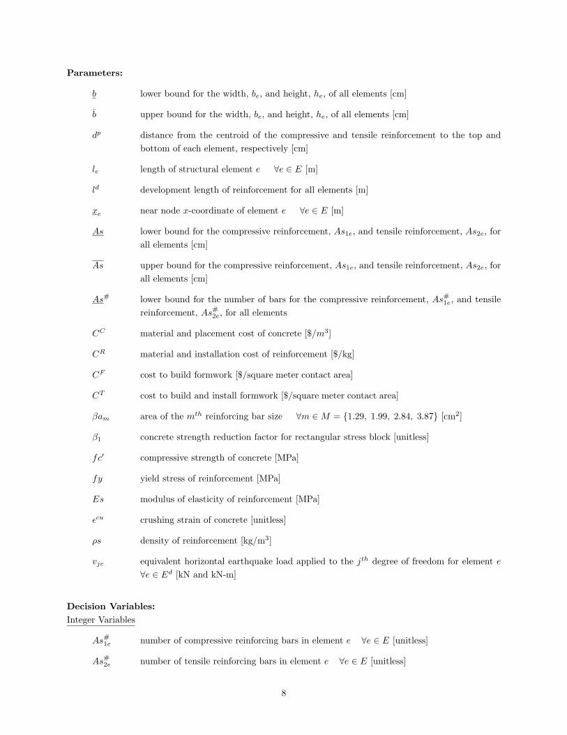
Parameters:

b lower bound for the width, be, and height, he, of all elements [cm]

b upper bound for the width, be, and height, he, of all elements [cm]

dp distance from the centroid of the compressive and tensile reinforcement to the top and

bottom of each element, respectively [cm]

le length of structural element e ∀e ∈ E [m]

ld development length of reinforcement for all elements [m]

xe near node x-coordinate of element e ∀e ∈ E [m]

As lower bound for the compressive reinforcement, As1e, and tensile reinforcement, As2e, for

all elements [cm]

As upper bound for the compressive reinforcement, As1e, and tensile reinforcement, As2e, for

all elements [cm]

As# lower bound for the number of bars for the compressive reinforcement, As#1e, and tensile

reinforcement, As#2e, for all elements

CC material and placement cost of concrete [$/m3]

CR material and installation cost of reinforcement [$/kg]

CF cost to build formwork [$/square meter contact area]

CT cost to build and install formwork [$/square meter contact area]

βam area of the mth reinforcing bar size ∀m ∈ M = {1.29, 1.99, 2.84, 3.87} [cm2]

β1 concrete strength reduction factor for rectangular stress block [unitless]

fc′ compressive strength of concrete [MPa]

fy yield stress of reinforcement [MPa]

Es modulus of elasticity of reinforcement [MPa]

ǫcu crushing strain of concrete [unitless]

ρs density of reinforcement [kg/m3]

vje equivalent horizontal earthquake load applied to the jth degree of freedom for element e

∀e ∈ Ed [kN and kN-m]

Decision Variables:

Integer Variables

As#1e number of compressive reinforcing bars in element e ∀e ∈ E [unitless]

As#2e number of tensile reinforcing bars in element e ∀e ∈ E [unitless]

8

Discrete Variables

be width of element e ∀e ∈ E [cm]

he height of element e ∀e ∈ E [cm]

As1e total compressive area of reinforcement in element e ∀e ∈ E [cm2]

As2e total tensile area of reinforcement in element e ∀e ∈ E [cm2]

Binary Variables

yem = 1 if the mth rebar size is used for element e ∀e ∈ Ex, ∀m ∈ M , 0 otherwise

we = 1 if the eth element formwork is already built ∀e ∈ Ex, 0 otherwise

zcee′ = 1 if column element e is the same size as column element e′ ∀e, e′ ∈ Ex ∩Ec ∋ e ≤ e′, 0

otherwise

zbee′ = 1 if beam element e is the same size as beam element e′ ∀e, e′ ∈ Ex ∩ Eb ∋ e ≤ e′, 0

otherwise

Auxiliary Variables

ce distance from the most compressive concrete fiber to the neutral axis for element e ∀e ∈

Ex [cm]

ce reduced distance from the most compressive concrete fiber to incorporate appropriate

concrete resistive strength of element e ∀e ∈ Ex [cm]

fed applied axial force, shear force, and bending moments at the dth degree of freedom for

element e ∀e ∈ E, ∀d ∈ De [kN and kN/m]

kedd′ stiffness between degrees of freedom d and d′ for element e ∀e ∈ E, ∀d, d′ ∈ De [kN and

kN/m]

Kdd′ stiffness between the free degrees of freedom d and d′ ∀d, d′ ∈ Df [kN and kN/m]

qed equivalent nodal load for the dth degree of freedom for element e with distributed loads

∀e ∈ Ed, ∀d ∈ De [kN and kN-m]

Qd nodal load for the dth free degree of freedom ∀d ∈ Df [kN and kN-m]

s+e positive slack variable for determining strain in the tensile reinforcement in element e

∀e ∈ E [unitless]

s−e negative slack variable for determining strain in the tensile reinforcement in element e

∀e ∈ E [unitless]

Te slack variable for minimum applied axial force requirements in element e ∀e ∈ E [MPa]

∆d nodal displacement for the dth free global degree of freedom ∀d ∈ Df [m]

δed nodal displacement at the dth global degree of freedom for element e ∀e ∈ E ∀d ∈ De

[m]

9

φe ACI strength reduction factor for element e ∀e ∈ Ex [unitless]

ǫse strain in the compressive reinforcement for element e ∀e ∈ Ex [unitless]

ǫte strain in the tensile reinforcement for element e ∀e ∈ Ex [unitless]

ǫse strain in compressive reinforcement of element e that remains within yield strain limits

∀e ∈ Ex [unitless]

ǫte strain in tensile reinforcement of element e that remains within yield strain limits ∀e ∈

Ex [unitless]

ǫφe strain in tensile reinforcement of element e to formulate the strength reduction factor, φe

[unitless]

ude factored distributed load including the self weight of element e ∀e ∈ Ed [kN/m]

xe location of the plastic centroid from the most compressive concrete fiber ∀e ∈ E [cm]

We now state the full model before commenting on some of its aspects in detail.

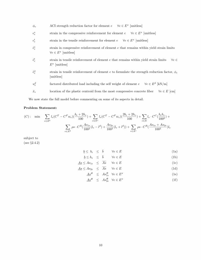
Problem Statement:

(C) : min∑

e∈Eb

le(CT − CFwe)(

be + 2he100

) +∑

e∈Ec

le(CT − CFwe)(

2be + 2he100

) +∑

e∈E

le · CC(

behe1002

) +

∑

e∈Eb

ρs · CR(As1e1002

(le − ld) +As2e1002

(le + ld)) +∑

e∈Ec

ρs · CR(As1e +As2e

1002)le

subject to

(see §2.4.2)

b ≤ be ≤ b ∀e ∈ E (1a)

b ≤ he ≤ b ∀e ∈ E (1b)

As ≤ As1e ≤ As ∀e ∈ E (1c)

As ≤ As2e ≤ As ∀e ∈ E (1d)

As# ≤ As#1e ∀e ∈ Ex (1e)

As# ≤ As#2e ∀e ∈ Ex (1f)

10

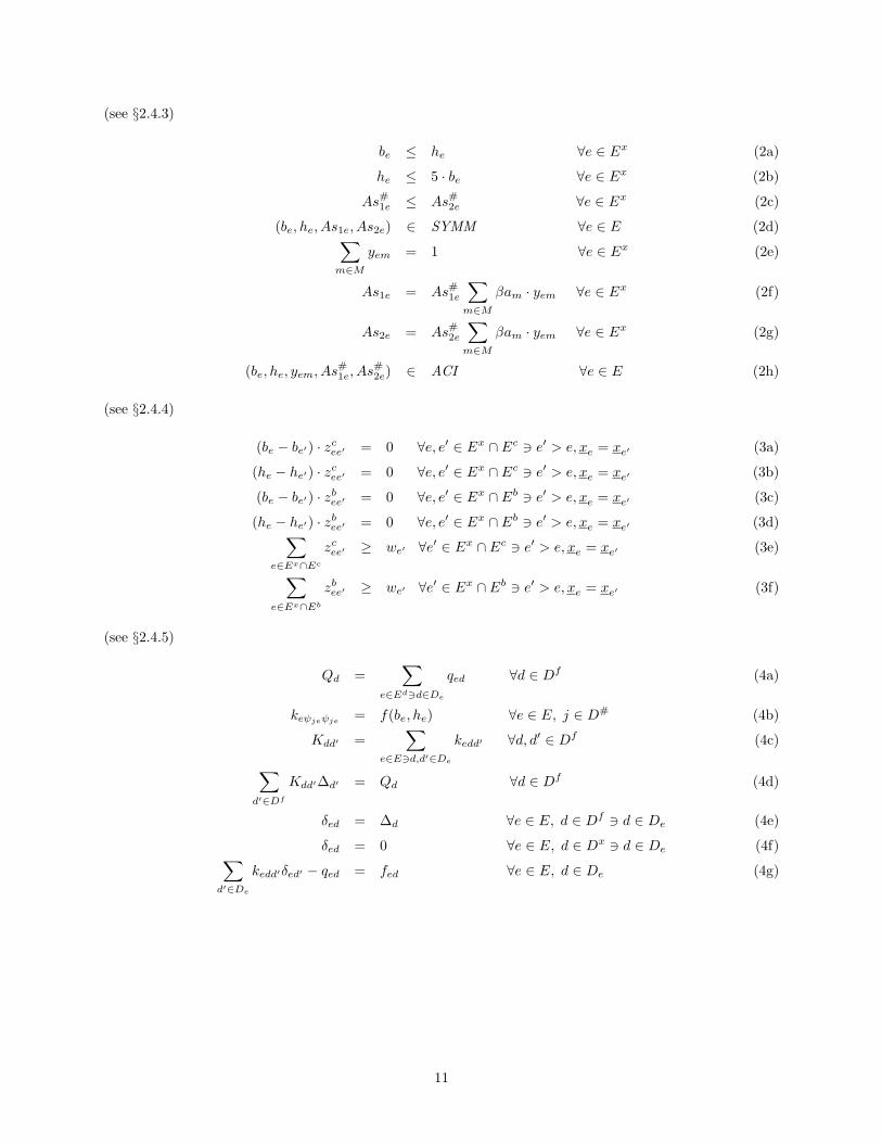
(see §2.4.3)

be ≤ he ∀e ∈ Ex (2a)

he ≤ 5 · be ∀e ∈ Ex (2b)

As#1e ≤ As#2e ∀e ∈ Ex (2c)

(be, he, As1e, As2e) ∈ SYMM ∀e ∈ E (2d)∑

m∈M

yem = 1 ∀e ∈ Ex (2e)

As1e = As#1e∑

m∈M

βam · yem ∀e ∈ Ex (2f)

As2e = As#2e∑

m∈M

βam · yem ∀e ∈ Ex (2g)

(be, he, yem, As#1e, As#2e) ∈ ACI ∀e ∈ E (2h)

(see §2.4.4)

(be − be′) · zcee′ = 0 ∀e, e′ ∈ Ex ∩ Ec ∋ e′ > e, xe = xe′ (3a)

(he − he′) · zcee′ = 0 ∀e, e′ ∈ Ex ∩ Ec ∋ e′ > e, xe = xe′ (3b)

(be − be′) · zbee′ = 0 ∀e, e′ ∈ Ex ∩ Eb ∋ e′ > e, xe = xe′ (3c)

(he − he′) · zbee′ = 0 ∀e, e′ ∈ Ex ∩ Eb ∋ e′ > e, xe = xe′ (3d)

∑

e∈Ex∩Ec

zcee′ ≥ we′ ∀e′ ∈ Ex ∩ Ec ∋ e′ > e, xe = xe′ (3e)

∑

e∈Ex∩Eb

zbee′ ≥ we′ ∀e′ ∈ Ex ∩ Eb ∋ e′ > e, xe = xe′ (3f)

(see §2.4.5)

Qd =∑

e∈Ed∋d∈De

qed ∀d ∈ Df (4a)

keψjeψje= f(be, he) ∀e ∈ E, j ∈ D# (4b)

Kdd′ =∑

e∈E∋d,d′∈De

kedd′ ∀d, d′ ∈ Df (4c)

∑

d′∈Df

Kdd′∆d′ = Qd ∀d ∈ Df (4d)

δed = ∆d ∀e ∈ E, d ∈ Df ∋ d ∈ De (4e)

δed = 0 ∀e ∈ E, d ∈ Dx ∋ d ∈ De (4f)∑

d′∈De

kedd′δed′ − qed = fed ∀e ∈ E, d ∈ De (4g)

11

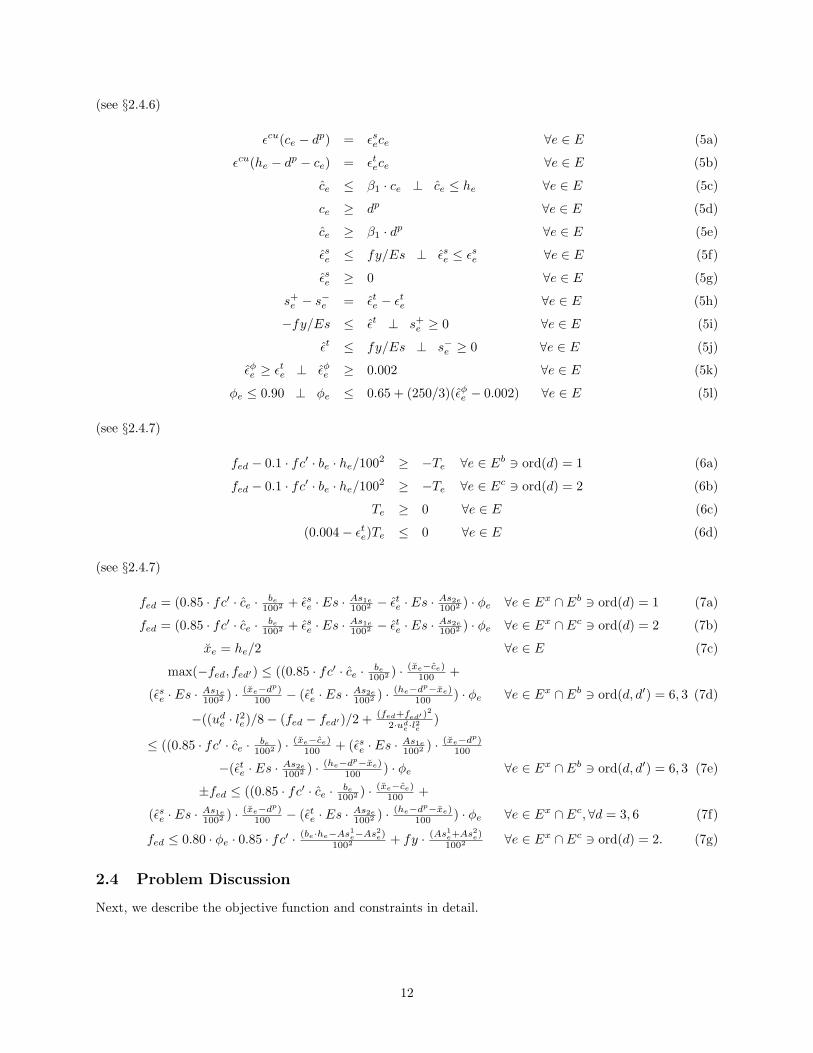
(see §2.4.6)

ǫcu(ce − dp) = ǫsece ∀e ∈ E (5a)

ǫcu(he − dp − ce) = ǫtece ∀e ∈ E (5b)

ce ≤ β1 · ce ⊥ ce ≤ he ∀e ∈ E (5c)

ce ≥ dp ∀e ∈ E (5d)

ce ≥ β1 · dp ∀e ∈ E (5e)

ǫse ≤ fy/Es ⊥ ǫse ≤ ǫse ∀e ∈ E (5f)

ǫse ≥ 0 ∀e ∈ E (5g)

s+e − s−e = ǫte − ǫte ∀e ∈ E (5h)

−fy/Es ≤ ǫt ⊥ s+e ≥ 0 ∀e ∈ E (5i)

ǫt ≤ fy/Es ⊥ s−e ≥ 0 ∀e ∈ E (5j)

ǫφe ≥ ǫte ⊥ ǫφe ≥ 0.002 ∀e ∈ E (5k)

φe ≤ 0.90 ⊥ φe ≤ 0.65 + (250/3)(ǫφe − 0.002) ∀e ∈ E (5l)

(see §2.4.7)

fed − 0.1 · fc′ · be · he/1002 ≥ −Te ∀e ∈ Eb ∋ ord(d) = 1 (6a)

fed − 0.1 · fc′ · be · he/1002 ≥ −Te ∀e ∈ Ec ∋ ord(d) = 2 (6b)

Te ≥ 0 ∀e ∈ E (6c)

(0.004− ǫte)Te ≤ 0 ∀e ∈ E (6d)

(see §2.4.7)

fed = (0.85 · fc′ · ce ·be

1002 + ǫse · Es · As1e1002 − ǫte · Es · As2e1002 ) · φe ∀e ∈ Ex ∩ Eb ∋ ord(d) = 1 (7a)

fed = (0.85 · fc′ · ce ·be

1002 + ǫse · Es · As1e1002 − ǫte · Es · As2e1002 ) · φe ∀e ∈ Ex ∩ Ec ∋ ord(d) = 2 (7b)

xe = he/2 ∀e ∈ E (7c)

max(−fed, fed′) ≤ ((0.85 · fc′ · ce ·be

1002 ) ·(xe−ce)

100 +

(ǫse · Es · As1e1002 ) ·(xe−d

p)100 − (ǫte · Es · As2e1002 ) ·

(he−dp−xe)

100 ) · φe ∀e ∈ Ex ∩ Eb ∋ ord(d, d′) = 6, 3 (7d)

−((ude · l2e)/8− (fed − fed′)/2 +

(fed+fed′ )2

2·ude ·l

2e

)

≤ ((0.85 · fc′ · ce ·be

1002 ) ·(xe−ce)

100 + (ǫse · Es · As1e1002 ) ·(xe−d

p)100

−(ǫte · Es · As2e1002 ) ·(he−d

p−xe)100 ) · φe ∀e ∈ Ex ∩ Eb ∋ ord(d, d′) = 6, 3 (7e)

±fed ≤ ((0.85 · fc′ · ce ·be

1002 ) ·(xe−ce)

100 +

(ǫse · Es · As1e1002 ) ·(xe−d

p)100 − (ǫte · Es · As2e1002 ) ·

(he−dp−xe)

100 ) · φe ∀e ∈ Ex ∩ Ec, ∀d = 3, 6 (7f)

fed ≤ 0.80 · φe · 0.85 · fc′ ·

(be·he−As1

e−As2

e)1002 + fy ·

(As1e+As2

e)1002 ∀e ∈ Ex ∩ Ec ∋ ord(d) = 2. (7g)

2.4 Problem Discussion

Next, we describe the objective function and constraints in detail.

12

2.4.1 Objective Function

The objective function includes, in order of appearance, formwork cost for all elements, concrete cost for all

elements, and reinforcement cost for all elements. We separate formwork costs into terms for beams and

columns because columns require formwork on all four sides whereas beams require formwork on only three

sides. Similarly, we develop reinforcement costs with terms for beams and columns because the length of

reinforcement relative to the element length is different for beams and columns. We utilize binary variables,

we, in the objective function, as explained in Section 2.4.4, to develop a cost model for formwork reuse that

follows the estimating methods of RC construction companies.

2.4.2 Upper and Lower Variable Bounds

Constraints (1a) through (1d) define lower and upper bounds on the variables that describe the cross-section

dimensions of each element e. Constraints (1e) and (1f) incorporate lower bounds for the number of bars for

the compressive and tensile reinforcement, As#1e and As#2e.

2.4.3 Geometry Restrictions

While constraint (2a) ensures that the width is less than the height, constraint (2b) prevents the creation of

tall, slender elements and maintains dimensions corresponding to typical behavior for beams and columns.

Constraint (2c) ensures that the area of tensile reinforcement is always greater than the area of compressive

reinforcement to maintain flexible elements. Constraint (2d) restricts all symmetric elements with respect to

horizontal location to contain the same width, height, and reinforcement area. Constraints (2e) through (2g)

define a special ordered set for selecting a discrete reinforcement bar size from the set of |M | sizes, where

the parameter βam is the cross-sectional area for the mth bar size. Constraint (2h) enforces reinforcing bar

spacing and percentage requirements based on ACI code specifications.

2.4.4 Formwork Reuse

Nonlinear equality constraints (3a) and (3b) restrict the formwork reuse binary variables for columns, zcee′ ,

to equal 1 if and only if the column element e has the same width and height as a column element, e′, on a

higher story level, indicated by a larger element number, with the same horizontal ordinate (xe). The same

convention follows for beam elements in constraints (3c) and (3d). When columns or beams, respectively, on

a higher story level contain the same width and height as columns or beams on a lower story level, formwork

costs are substantially lower because formwork is reused. While constraints (3a) through (3d) compare the

dimensions of elements on each story level, constraints (3e) and (3f) define the binary variable, we, in terms

of the values of the binary variables zcee′ and zbee′ . Essentially, constraints (3e) and (3f) allow we to equal 1

if a beam or column element, respectively, on a higher story level contains the same dimensions as a beam

or column on any lower story level. Note that we force columns that are symmetrically located about the

horizontal midpoint of the structure to have equal cross-section width and height.

2.4.5 Finite Element Analysis

Constraints (4a) through (4g) define the relations between stiffness, applied forces, and displacements for

finite element analysis with beam and column elements. Constraint (4a) defines the equivalent nodal loads

for all elements in the structure based on equivalent nodal loads for each element. Equation (4b) defines the

element stiffnesses as a function of element widths and heights. Element stiffness is a highly nonlinear function

of the element widths and depths. Constraint (4c) assembles the global stiffnesses at each degree of freedom

13

d and d′ from element stiffnesses, kedd′ . Constraint (4d) defines equilibrium of forces, displacements, and

stiffnesses for the finite element analysis. Constraint (4e) defines the nodal displacements for each element by

extracting the appropriate values from the displacement vector, ∆d. Constraint (4f) sets the displacements

at each fixed degree of freedom to zero. Constraint (4g) defines internal forces, fed, at the dth degree of

freedom for element e. The internal forces include the shear, axial, and bending moments at the two nodes

in each beam and column element. Further details about the finite element analysis can be found in Guerra

(2008).

2.4.6 Resistive Forces: Complementarity Constraints

While the finite element analysis provides demand in terms of bending and axial forces that must be resisted

in each element, constraints (5a) through (5l) express the capacity in terms of bending and axial forces that

each element can resist. In order to meet structural stability, which is discussed in Section 2.4.7, the resistive

capacity must be greater than or equal to the demand in each element. Constraints (5a) and (5b) define

a linear strain distribution across the height of each element in order to determine the resistive capacity

of the reinforced cross-section. Complementarity constraints (5c) through (5e) ensure appropriate concrete

compressive resistance when the entire cross-section contains compressive strains and when only a portion

of the cross-section contains compressive strains. (See the left hand side of Figure 3.) Complementarity

constraints (5f) and (5g) define elastic-perfectly plastic material response for the resistive capacity of the

compressive reinforcement when the strain in the compressive reinforcement is less than and greater than

the yield strain. Elastic-perfectly plastic material response ensures that the maximum resistive capacity

corresponds to the yield strain. (See the first quadrant of the right hand side of Figure 3.) Complementarity

constraints (5h) through (5j) define elastic-perfectly plastic material response for the resistive capacity of

the tensile reinforcement using positive and negative slack variables, s+e and s−e , respectively. (See Figure

3 in its entirety.) Complementarity constraints (5k) and (5l) define the appropriate value for the strength

reduction factor according to ACI code requirements as a function of the strain in the tensile reinforcement.

The strength reduction factor incorporates factors of safety into the design. (See the left hand side of Figure

4.)

2.4.7 Restrictions for Structural Stability

In general, in order to maintain structural stability, the capacity of each element must be greater than the

demand. Constraints (6a) through (6d) enforce ACI code requirements for minimum eccentricity of applied

forces using conditional complementarity depending on the value of a slack variable, Te. For situations in

which the strain in the tensile reinforcement is greater than or equal to 0.004 (an ACI-specified value), there

is sufficient bending in the element, the value of the slack variable must only be greater than or equal to

zero, conditional complementarity is not invoked, and requirements for minimum eccentricity do not apply.

For situations in which the strain in the tensile reinforcement is less than 0.004, the value of Te must equal

zero, and the applied axial force must be greater than 10 percent of the maximum axial concrete resistance.

(See the right hand side of Figure 4.)

Constraints (7a) and (7b) restrict the resistive axial force of the cross-section to be equal to the applied

axial force in each beam and column element, respectively. Because the bending resistive force can increase

with increasing applied axial forces, equality of the resistive and applied forces ensures that the magnitude

of the resistive bending force corresponds to the appropriate applied axial force. Constraint (7c) defines

the location of the plastic centroid from the most compressive concrete fiber, which represents the point

about which the bending resistance is computed. Constraints (7d) and (7e) enforce that the corresponding

14

)100/('85.0 ebfc ��

)100/(1 ec�E

(meters)

Concrete Resistive Force

(kN)

eh /100

2100

)Ö('85.0 ee bcfc ���

fy

Esfy /

Strain in Tensile Reinforcement,

Esfy /�

fy�

Es

Stress in Tensile Reinforcement

(Mpa)

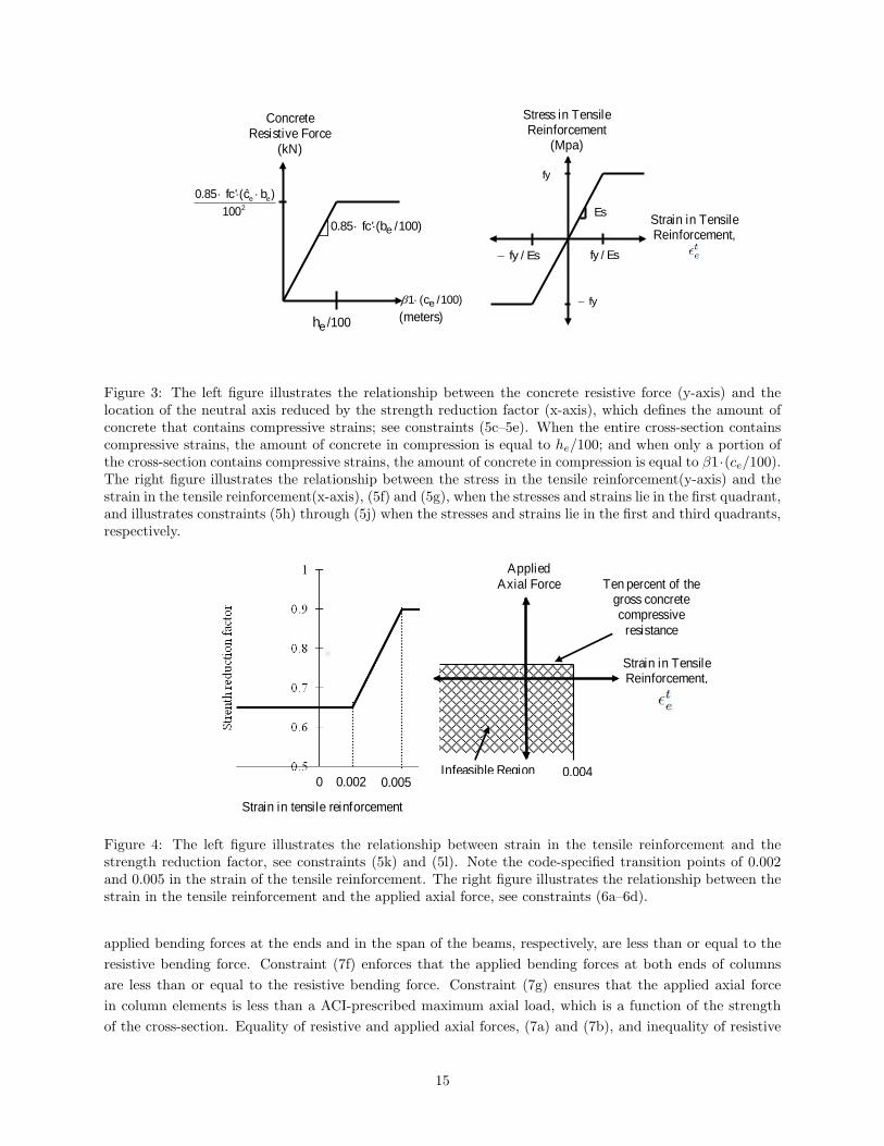
Figure 3: The left figure illustrates the relationship between the concrete resistive force (y-axis) and thelocation of the neutral axis reduced by the strength reduction factor (x-axis), which defines the amount ofconcrete that contains compressive strains; see constraints (5c–5e). When the entire cross-section containscompressive strains, the amount of concrete in compression is equal to he/100; and when only a portion ofthe cross-section contains compressive strains, the amount of concrete in compression is equal to β1·(ce/100).The right figure illustrates the relationship between the stress in the tensile reinforcement(y-axis) and thestrain in the tensile reinforcement(x-axis), (5f) and (5g), when the stresses and strains lie in the first quadrant,and illustrates constraints (5h) through (5j) when the stresses and strains lie in the first and third quadrants,respectively.

0.004

Applied Axial Force

Infeasible Region

Ten percent of the gross concrete compressive

resistance

Strain in Tensile Reinforcement,

0.005 0.002

Strain in tensile reinforcement

0

Figure 4: The left figure illustrates the relationship between strain in the tensile reinforcement and thestrength reduction factor, see constraints (5k) and (5l). Note the code-specified transition points of 0.002and 0.005 in the strain of the tensile reinforcement. The right figure illustrates the relationship between thestrain in the tensile reinforcement and the applied axial force, see constraints (6a–6d).

applied bending forces at the ends and in the span of the beams, respectively, are less than or equal to the

resistive bending force. Constraint (7f) enforces that the applied bending forces at both ends of columns

are less than or equal to the resistive bending force. Constraint (7g) ensures that the applied axial force

in column elements is less than a ACI-prescribed maximum axial load, which is a function of the strength

of the cross-section. Equality of resistive and applied axial forces, (7a) and (7b), and inequality of resistive

15

and applied bending forces, (7d–7f), ensure that the applied axial and bending forces fall within the locus

of failure for any feasible combination of axial and bending forces. Constraint (7g) enforces an upper bound

on the applied axial force.

2.4.8 Fixed Case of Formwork Reuse Constraints

We can reduce the combinatorial complexity of the problem by adding logical constraints that force a

particular formwork reuse. We do so by fixing the binary variables zcee′ and zbee′ to a value of 0 or 1 to force

a particular formwork reuse distribution. We include formwork distributions such that all columns contain

the same dimensions and all beams contain the same dimensions by forcing: zcee′ = 1 ∀e, e′ ∈ Ex ∩ Ec ∋

e′ > e, xe = xe′ and zbee′ = 1 ∀e, e′ ∈ Ex ∩ Eb ∋ e′ > e, xe = xe′ . We also include formwork distributions in

which subsets of beams and columns contain the same dimensions, by forcing a subset of the binary variable

values to 1 and the remaining values to 0. For example, for eight stories, we force two to be one size and

six to be another, three to be one size and five to be another; for three form sizes we force, for example,

two stories to be one size, two to be another, and four to be yet another. Forcing values for these binary

variables eliminates the associated nonlinear equality and inequality constraints (3a–3f) in the formulation.

In Section 4, we compare the algorithm performance for the fixed case of the formulation, which contains

additional restrictions, and the free case of the formulation, which does not contain additional restrictions

on the binary variables.

2.4.9 Potential Convex Reformulations

Rather than using nonlinear constraints as shown in (3a–3f), we also examine the effect on model tractability

of a convex hull formulation for formwork reuse. Unfortunately, this reformulation does not result in faster

solve times; we give this reformulation in the appendix.

In addition, we study a convex reformulation of the nonlinear equality constraints (2f) and (2g) by

replacing them with the following linear constraints:

−2 ·As · (1− yem) ≤ As1e − βam ·As#1e ≤ 2 ·As · (1− yem) ∀e ∈ Ex, ∀m ∈ M (8a)

−2 ·As · (1− yem) ≤ As2e − βam ·As#2e ≤ 2 ·As · (1− yem) ∀e ∈ Ex, ∀m ∈ M (8b)

which is a big-M formulation.

3 Model Instances

We include two-dimensional design examples for one-bay structures with one- to eight-story levels. We use

beam lengths of five meters, typical for RC structures, and a load case with both horizontal and vertical loads

to demonstrate optimal solutions for combinations of applied axial force and bending moment magnitudes

that cover a wide range of values typically observed in RC elements.

3.1 Parameter Values

The parameters in this study contain common values used in the design of RC structures. Table 1 presents

the material properties used for all examples. All structures are loaded by their self weight, wG, an additional

gravity dead load, wD = 30kN/m, and a gravity live load, wL = 30kN/m, which are typical values for office

buildings. We calculate the parameters that describe horizontal seismic forces, vje, for the jth degree of

16

freedom for element e using the ASCE 7 (SEI/ASCE 7-98) equivalent lateral load procedure for a structure

in Denver, Colorado, the failure of which would result in a substantial public hazard. Buildings subjected to

gravity and seismic loads contain factored loads of 1.2wG+1.2wD+1.0wL+1.0vje = 1.2wG+66kN/m+1.0vje.

Table 2 summarizes the values of the seismic horizontal forces for the multistory design examples with beam

lengths of five meters. For all examples, the horizontal loads increase for each story level so that the top

story level contains the largest horizontal load.

Table 1: Material properties for concrete and reinforcement

Description Parameter Name Value UnitsLower bound for the width and depth of elements b 20 cmUpper bound for the width and depth of elements b 200 cmConcrete cover dp 7 cmLength of structural element e le 3-10 mDevelopment length of reinforcement ld 1.11 mNear node x-coordinate of element e xe 0-20 mLower bound for reinforcement As 2.58 cmUpper bound for reinforcement As 2.58 cm

Lower bound for the number of reinforcing bars As# 2 unitlessMaterial and placement unit price of concrete CC 192.80 $/m3

Material and installation unit price of reinforcement CR 1.55 $/kgUnit price to build formwork CF 32.60 $/SMCAUnit price to build and install formwork CT 38.00 $/SMCAACI Section 10.2.7.3 reduction factor β1 0.85 unitlessConcrete compressive strength fc′ 28 MPaReinforcement yield stress fy 420 MPaReinforcement modulus of elasticity Es 200,000 MPaCrushing strain of concrete ǫcu 0.003 unitlessDensity of reinforcement ρs 7870 kg/m3

Table 2: Horizontal loads for spans of five meters

Total Horizontal Load on Story Level:Number of One Two Three Four Five Six Seven EightStory Levels (kN) (kN) (kN) (kN) (kN) (kN) (kN) (kN)1 15.6 – – – – – – –2 10.4 20.8 – – – – – –3 7.8 15.6 23.4 – – – – –4 6.3 12.5 18.8 25.0 – – – –5 4.8 9.9 14.9 20.0 25.1 – – –6 3.3 6.9 10.7 14.5 18.4 22.3 – –7 2.3 5.0 7.9 10.9 13.2 17.0 20.2 –8 1.9 3.8 6.2 8.6 11.1 13.6 16.3 19.0

3.2 Initialization of Variables

Initial variable values provide a starting point for the algorithm and strongly influence the performance. We

set an initial value for all variables in the optimization formulation based on a typical design practice that

17

meets all the constraints in the problem formulation. This “typical solution” provides a feasible starting point

and can be compared with solutions from MINLPBB to determine cost savings potential for the structures

we consider. We develop the typical solution with a method often used in practice: (1) approximate an

initial width and depth of beam and column elements using applied loads and beams lengths, (2) determine

the applied forces and moments on each element using finite element analysis, (3) determine the number and

size of reinforcing bars to resist applied forces and moments, and (4) determine whether the number and size

of reinforcing bars fits within the cross-section with required spacing and concrete cover. If the reinforcement

does not fit, then element widths and/or depths are increased in five-centimeter increments and we repeat

steps 2 through 4. While we could use various initial variable values and compare the corresponding objective

function values to find the best locally optimal solution, we use only the initial variable values from the typical

solution.

3.3 Problem Size and Structure

The mathematical structure of the RC design problem is highly nonlinear and nonconvex. Discrete-valued

variables describe constructible design solutions and continuous-valued variables model material response.

Nonlinear equality and complementarity constraints make the problem nonconvex. We present information

about the size of the problems in terms of the number of story levels, number of variables (including integer

variables), number of constraints (including nonlinear constraints) and number of complementarity constraint

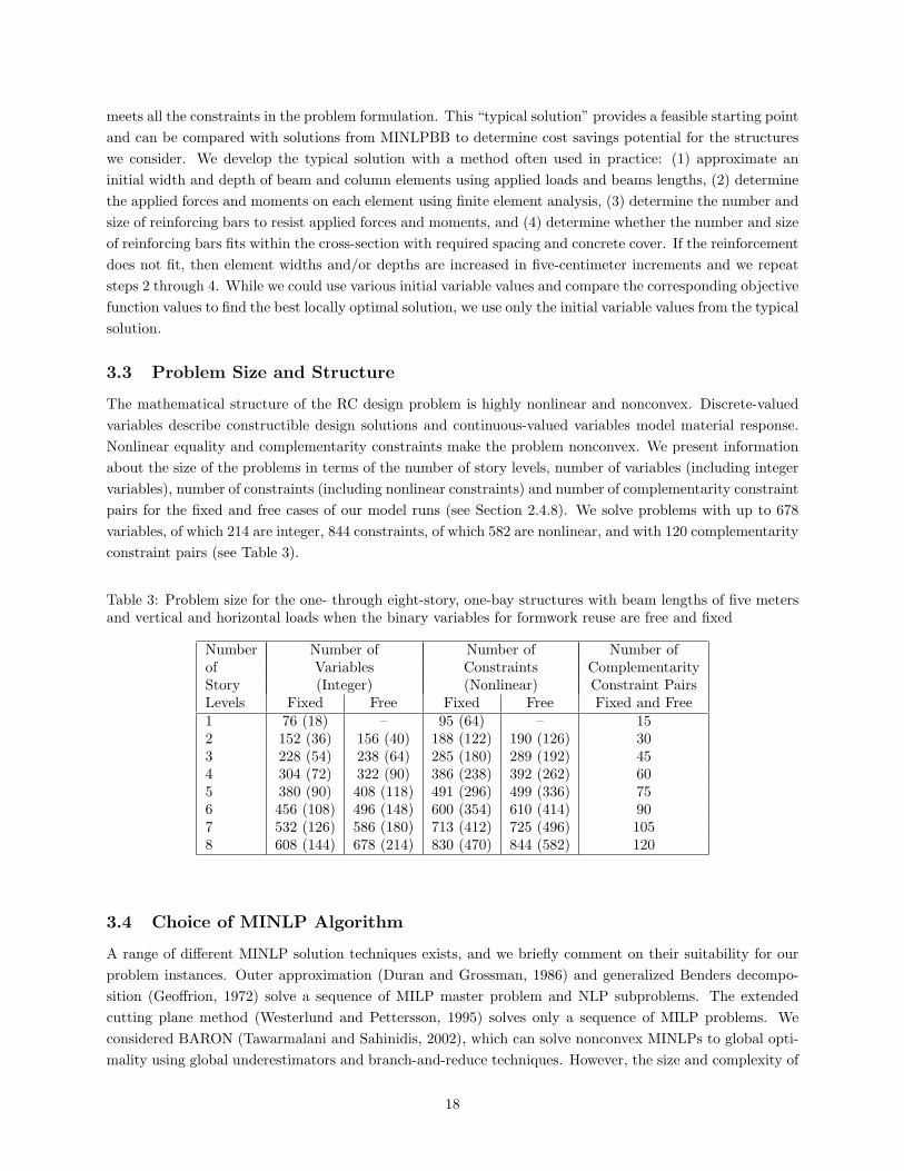
pairs for the fixed and free cases of our model runs (see Section 2.4.8). We solve problems with up to 678

variables, of which 214 are integer, 844 constraints, of which 582 are nonlinear, and with 120 complementarity

constraint pairs (see Table 3).

Table 3: Problem size for the one- through eight-story, one-bay structures with beam lengths of five metersand vertical and horizontal loads when the binary variables for formwork reuse are free and fixed

Number Number of Number of Number ofof Variables Constraints ComplementarityStory (Integer) (Nonlinear) Constraint PairsLevels Fixed Free Fixed Free Fixed and Free1 76 (18) – 95 (64) – 152 152 (36) 156 (40) 188 (122) 190 (126) 303 228 (54) 238 (64) 285 (180) 289 (192) 454 304 (72) 322 (90) 386 (238) 392 (262) 605 380 (90) 408 (118) 491 (296) 499 (336) 756 456 (108) 496 (148) 600 (354) 610 (414) 907 532 (126) 586 (180) 713 (412) 725 (496) 1058 608 (144) 678 (214) 830 (470) 844 (582) 120

3.4 Choice of MINLP Algorithm

A range of different MINLP solution techniques exists, and we briefly comment on their suitability for our

problem instances. Outer approximation (Duran and Grossman, 1986) and generalized Benders decompo-

sition (Geoffrion, 1972) solve a sequence of MILP master problem and NLP subproblems. The extended

cutting plane method (Westerlund and Pettersson, 1995) solves only a sequence of MILP problems. We

considered BARON (Tawarmalani and Sahinidis, 2002), which can solve nonconvex MINLPs to global opti-

mality using global underestimators and branch-and-reduce techniques. However, the size and complexity of

18

the nonlinear expressions in the finite element analysis make it unlikely that BARON can succeed in solving

our problem (Sahinidis, 2006). All four methods rely heavily on the convexity of the problem functions or

the ready availability of underestimators. Unfortunately, our models do not easily admit underestimators,

and we cannot apply these techniques. We also considered using NOMADm (Abramson, 2005, 2006), a

pattern search technique that does not require derivative information (Torczon, 1997).

An alternative to these techniques is nonlinear branch-and-bound. This method solves a sequence of

nonlinear problems at every node of a tree. One advantage of this approach is that nonlinear solvers often find

good solutions even to nonconvex problems. The MINLPBB solver is attractive because the underlying SQP

method has been shown to be an efficient and robust solver for optimization problems with complementarity

constraints (Fletcher and Leyffer, 2004).

We solve the RC design problem with a software package, MINLPBB (Leyffer 1999), on Linux-based

servers with dual-core AMD Opteron processors with a CPU speed of 2.41 GHz and random access memory

of approximately one gigabyte. MINLPBB uses a branch-and-bound framework with a sequential quadratic

programming technique to solve the continuous relaxations of the problem (Fletcher and Leyffer, 1998;

Leyffer, 1999; Leyffer, 2001). The branch and bound method in MINLPBB uses a depth-first search and

solves the NLP relaxations using filterSQP (Fletcher and Leyffer, 1998). The user can influence branching by

supplying priorities for integer variables, as well as by choosing node selection strategies and branching rules

(Leyffer, 1999). We use a depth-first search strategy, branching on the variable with the highest user-defined

priority. MINLPBB guarantees global optimality only for convex problems. However, it also provides a

more robust solution technique for nonconvex MINLP problems in comparison to outer approximation and

Benders decomposition (Leyffer, 1999). Outer approximation and Benders decomposition often reduce the

size of the feasible region by using cuts, which can eliminate optimal solutions in nonconvex problems like

our RC design problem. Fletcher and Leyffer (2004) have demonstrated the abilities of the NLP solver in

MINLPBB, filterSQP, to solve over 150 optimization problems with complementarity constraints.

4 Numerical Results

We present design examples to illustrate three key aspects: (1) MINLPBB algorithm performance for the

RC design problem, (2) cost savings over typical practice, and (3) characteristics of the optimal solution,

namely, optimal formwork reuse and stiffness distributions. We detail these aspects and the corresponding

results in the following three subsections.

4.1 Algorithm Performance

Recall that we solve two cases of the optimization formulation: the original formulation that allows solutions

with any formwork reuse distribution, termed the free case, and the formulation that contains restrictions

that enforce a particular formwork reuse distribution, the fixed case. While we find solutions for up to an

eight-story, one-bay structure for the original problem formulation, we can find solutions in less CPU time

when a particular formwork reuse distribution is enforced. Figure 5 illustrates on a logarithmic scale the

CPU time as a function of the number of integer variables for both the fixed and free cases.

Table 4 summarizes the number of nonlinear programs solved and the algorithm performance (in terms of

solution time) for the the fixed and free cases for one-bay structures with up to eight story levels. In each case,

we run MINLPBB until termination or until we reach a memory limit. The fixed cases require significantly

less CPU time, on average, than do the free cases. As expected, the CPU time increases exponentially as

the problem size increases in both cases. In the fixed case, however, the amount of CPU time is less than

19

Figure 5: Number of nonlinear programs solved to reach the optimal solution vs. number of integer variablesfor the one-bay structures for the fixed case of the optimization formulation

two hours for the eight-story scenario, whereas for the free case, the largest scenario requires days of CPU

time.

We study a convex formulation of constraints (2f) and (2g), which is a special ordered set formulation,

using a Big-M construct; see constraints (8a) and (8b). As expected, the objective function value is the same

as that of the original formulation. However, the CPU time is about 100 times longer than that resulting

from the special ordered set formulation for the three-story one-bay structure with vertical loads only. We

also study the convex formulation of constraints (3a) through (3f), which are nonlinear equality constraints,

using a convex hull formulation (see the appendix). The objective function value for the NLP relaxation

of the convex hull is slightly lower than the NLP relaxation of the original formulation, indicating a looser

lower bound. The objective function value for the convex hull formulation is the same as that of the original

formulation. However, the CPU time for the three-story case is about 375 times longer than that of the

original formulation with nonlinear equality constraints.

4.2 Objective Function Values

To justify the use of integer variables, we compare rounded solutions from the root node found with

MINLPBB and discrete-valued solutions from MINLPBB for the one- through eight-story, one-bay struc-

tures with beam lengths of five meters and vertical and horizontal loads. In both rounding and MINLP

methods, the initial variable values equal those of the typical solution. Additionally, rounding and branching

operations both begin from a root node in which the binary variables for formwork reuse are fixed such that

all beams contain the same dimensions and all columns contain the same dimensions. We also enforce this

formwork distribution in rounding operations. We allow the solver to determine discrete reinforcing bar sizes

before rounding.

We obtain an integer feasible solution by rounding as follows: (1) if element width and depth, be and he,

are continuous-valued, then round be and he up to the nearest five-centimeter increment; (2) if the number

of compressive and tensile reinforcing bars, As#1e and As#2e, are continuous-valued, then round up As#1e and

As#2e to the nearest integer value; (3) if the number and size of reinforcing bars does not fit with appropriate

cover and spacing, then round up be to the next five-centimeter increment; (4) if minimum reinforcement

ratios are violated, then round up the bar size to the next largest size or round up the number of bars if

20

already at largest bar size; (5) if maximum reinforcement ratios are violated, then round up be one increment

and, if needed after rounding be one increment, round up he one increment; (6) if the location of the neutral

axis is less than the lower bound of 7 centimeters, then round up the reinforcing bar size one increment, then

round up number of bars one increment, if needed, and then round up be one increment, if needed; (7) if the

bending force resistive capacity contains a smaller magnitude than the applied bending force, then round up

the bar size one increment and then he one increment, if needed; and (8) repeat steps 1 through 7 until a

feasible discrete solution is obtained.

To evaluate the relative quality of our solutions given various methods of increasing difficulty in obtaining

them, we make the following comparisons relative to the objective function value from a typical solution:

(1) the objective function value at the root node of the fixed case of the nonlinear programming relaxation;

(2) the objective function value from a rounded, feasible root node solution to the fixed problem; (3) the

objective function value found using MINLPBB with fixed formwork; and (4) the objective function value

found using MINLPBB allowing formwork reuse to vary. The last four columns of Table 4 show these results.

On average, the objective function value at the root node is 19 percent better (lower) than that provided

by the typical solution. We expect this marked contrast because the root node solution is not necessarily

integer feasible. On average, the solutions rounded from the fixed case show no improvement from the

typical solutions; some cases show a slight degradation, whereas others show a slight improvement. These

data demonstrate that rounding is not an effective means of improving on typical practice and underscores

the necessity of solving an integer nonlinear program to achieve savings over typical practice. The integer

feasible solution given by the fixed formwork case is 13 percent better than the typical solution, with no clear

trend in solution quality improvement as the number of story levels increases. The fixed solution generally

gives the same quality objective as the free solution, though the latter requires considerably more CPU time

to obtain. (In the largest two cases, the objective degrades slightly, indicating that an inferior local optimum

is found.) These results indicate that it is generally sufficient for these examples (cost structures) to consider

just the fixed case, though, in general, this would not be true.

Table 4: Number of nonlinear programs and the CPU time (seconds) for the fixed and free cases. Alsoreported are the percent savings over the typical solution (obtained heuristically) as given by the root nodesolution and the rounded solution (both heuristic solutions) and the local optimal solutions for the fixed andfree cases obtained with the MINLP solver.

Number of Number of CPU Time Percent Savings with Respect to Typical SolutionStory Levels Nonlinear Programs (seconds) Heuristic MINLP

Root Rounded Fixed FreeFixed Free Fixed Free Solution Solution Solution Solution

1 198 - 1 – 13.1 2.2 9.4 –2 239 284 4 5 19.1 -0.1 13.7 13.73 576 1637 20 56 22.0 0.8 16.0 16.04 1166 5133 84 357 21.4 2.6 14.2 14.95 2014 4776 215 562 20.6 4.9 13.9 13.96 7707 11038 1218 1527 18.9 -4.3 11.6 11.67 12611 55622 2651 14486 19.4 -2.4 12.2 11.68 18318 842945 5244 196606 18.0 0.7 10.6 10.2

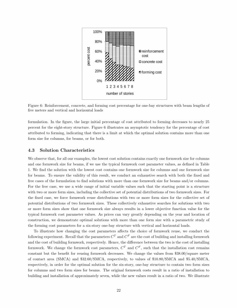
In Figure 6, we show the distribution of reinforcement, concrete, and forming costs for the one-bay

structures with beam lengths of five meters and vertical and horizontal loads for the fixed case of the

21

0%

20%

40%

60%

80%

100%

1 2 3 4 5 6 7 8pe

rcen

t cos

tnumber of stories

reinforcement cost

concrete cost

forming cost

Figure 6: Reinforcement, concrete, and forming cost percentage for one-bay structures with beam lengths offive meters and vertical and horizontal loads

formulation. In the figure, the large initial percentage of cost attributed to forming decreases to nearly 25

percent for the eight-story structure. Figure 6 illustrates an asymptotic tendency for the percentage of cost

attributed to forming, indicating that there is a limit at which the optimal solution contains more than one

form size for columns, for beams, or for both.

4.3 Solution Characteristics

We observe that, for all our examples, the lowest cost solution contains exactly one formwork size for columns

and one formwork size for beams, if we use the typical formwork cost parameter values, as defined in Table

1. We find the solution with the lowest cost contains one formwork size for columns and one formwork size

for beams. To ensure the validity of this result, we conduct an exhaustive search with both the fixed and

free cases of the formulation to find solutions with more than one formwork size for beams and/or columns.

For the free case, we use a wide range of initial variable values such that the starting point is a structure

with two or more form sizes, including the collective set of potential distributions of two formwork sizes. For

the fixed case, we force formwork reuse distributions with two or more form sizes for the collective set of

potential distributions of two formwork sizes. These collectively exhaustive searches for solutions with two

or more form sizes show that one formwork size always results in a lower objective function value for the

typical formwork cost parameter values. As prices can vary greatly depending on the year and location of

construction, we demonstrate optimal solutions with more than one form size with a parametric study of

the forming cost parameters for a six-story one-bay structure with vertical and horizontal loads.

To illustrate how changing the cost parameters affects the choice of formwork reuse, we conduct the

following experiment. Recall that the parameters CT and CF are the cost of building and installing formwork

and the cost of building formwork, respectively. Hence, the difference between the two is the cost of installing

formwork. We change the formwork cost parameters, CT and CF , such that the installation cost remains

constant but the benefit for reusing formwork decreases. We change the values from $38.00/square meter

of contact area (SMCA) and $32.60/SMCA, respectively, to values of $10.80/SMCA and $5.40/SMCA,

respectively, in order for the optimal solution for the six-story, one-bay structure to contain two form sizes

for columns and two form sizes for beams. The original formwork costs result in a ratio of installation to

building and installation of approximately seven, while the new values result in a ratio of two. We illustrate

22

139 kN-m

-100 kN-m

-84 kN-m

-104 kN-m

-130 kN-m

-118 kN-m

-186 kN-m

-232 kN-m

94 kN-m

183 kN

113 kN-m1217 kN

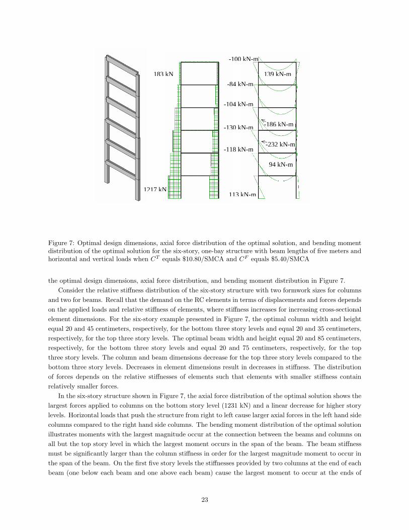
Figure 7: Optimal design dimensions, axial force distribution of the optimal solution, and bending momentdistribution of the optimal solution for the six-story, one-bay structure with beam lengths of five meters andhorizontal and vertical loads when CT equals $10.80/SMCA and CF equals $5.40/SMCA

the optimal design dimensions, axial force distribution, and bending moment distribution in Figure 7.

Consider the relative stiffness distribution of the six-story structure with two formwork sizes for columns

and two for beams. Recall that the demand on the RC elements in terms of displacements and forces depends

on the applied loads and relative stiffness of elements, where stiffness increases for increasing cross-sectional

element dimensions. For the six-story example presented in Figure 7, the optimal column width and height

equal 20 and 45 centimeters, respectively, for the bottom three story levels and equal 20 and 35 centimeters,

respectively, for the top three story levels. The optimal beam width and height equal 20 and 85 centimeters,

respectively, for the bottom three story levels and equal 20 and 75 centimeters, respectively, for the top

three story levels. The column and beam dimensions decrease for the top three story levels compared to the

bottom three story levels. Decreases in element dimensions result in decreases in stiffness. The distribution

of forces depends on the relative stiffnesses of elements such that elements with smaller stiffness contain

relatively smaller forces.

In the six-story structure shown in Figure 7, the axial force distribution of the optimal solution shows the

largest forces applied to columns on the bottom story level (1231 kN) and a linear decrease for higher story

levels. Horizontal loads that push the structure from right to left cause larger axial forces in the left hand side

columns compared to the right hand side columns. The bending moment distribution of the optimal solution

illustrates moments with the largest magnitude occur at the connection between the beams and columns on

all but the top story level in which the largest moment occurs in the span of the beam. The beam stiffness

must be significantly larger than the column stiffness in order for the largest magnitude moment to occur in

the span of the beam. On the first five story levels the stiffnesses provided by two columns at the end of each

beam (one below each beam and one above each beam) cause the largest moment to occur at the ends of

23

the beams. On the top story level in which the beam is attached only to one column at the end points, the

relative stiffness is such that the largest moment occurs in the span of the beam. The moment distribution

remains the same for the first five story levels because the relative stiffness of the beams and columns is

about the same for these story levels. This six-story example with two formwork sizes demonstrates the

range of stiffness distributions that we find for all other examples.

5 Conclusions

We present, for the first time, an explicit MINLP formulation of the RC design problem. We find optimal

solutions for RC structures that result in an average of 13 percent cost savings over the typical solution,

and we demonstrate the ability of MINLPBB to solve a new class of hard optimization problems: mixed

integer nonlinear problems with complementarity constraints. For the size of the problems considered in

this study, we find locally optimal solutions that contain one form size for columns and one form size for

beams. We find various distributions of relative element widths and depths, or stiffness, depending on the

structure size, geometry, and applied loads. In general, the most efficient concrete cross-section is one that

resists only compressive axial forces. The loads applied to multistory RC structures cause bending of the

elements, which creates elements of which only a portion of the concrete provides resistance.

Efficient designs for RC structures contain a large number of same-size elements to substantially reduce

formwork cost. For typical formwork unit prices we find optimal solutions with one form size and must

drastically decrease the unit price to find solutions with two form sizes. Further exploration of the transition

between one and two form sizes would provide a significant contribution to this research topic. Solving

systems with a larger number of story levels is necessary to explore such a transition. We find that the

performance of MINLPBB is affected by the number of variables and constraints and by the number of

different size cross-sections that must be determined. We find a decrease in the number of NLPs solved and

CPU time for the fixed case of the optimization formulation in comparison to the free case. We also find that

the free and fixed cases result in nearly the same quality of solutions. While the fixed case contains a smaller

number of integer variables, number of NLPs solved, and CPU time than does the free case, we find that

the fixed case quickly reaches a very large number of NLPs and CPU time. We show the limits of attainable

results when using MINLPBB for the RC design problem and find that we can solve one-bay structures with

up to eight story levels. To find solutions for structures with a larger number of story levels, we suggest

reducing the number of integer and binary variables and improving the branching scheme. One method to

reduce the number of integer and binary variables in the RC design problem without losing model fidelity

would be to describe the cross-section width and depth of a group of elements with only two variables so

that all elements in the group contain the same dimensions. Although the method would require a dynamic

group of elements in order to find the optimal number of elements that should contain the same dimensions,

the large number of same-size elements indicates that there is always some formwork reuse. Improvements

to the branching scheme could also increase tractability for larger problems. Any improvements to the

branching scheme in reference to the behavior of the RC design problem could substantially increase the

tractability of the RC design problem and allow the solution of instances with a larger number of degrees of

freedom. A sensitivity study of the variables in the problem could be used to determine the best types of

improvements for the branching scheme specific to the RC design problem. A better understanding of the

algorithm performance for the RC design problem could also help improve the branching scheme.

24

Acknowledgments

This work was supported by the Office of Advanced Scientific Computing Research, Office of Science, U.S.

Department of Energy, under Contract DE-AC02-06CH11357 and through the grant DE-FG02-05ER25694.

The authors are also grateful to Professor Panos Kiousis in the Engineering Division at the Colorado School

of Mines for introducing this problem to us.

A Convex Hull Reformulation

We replace the nonlinear equality constraints given in (3a–3f) with the convex hull formulation for formwork

reuse, as shown below.

k ∈ K set of sizes for element width and depth, be and he, respectively

Binary Variables

zbek =

{

1 if the kth size is used for the width of element e ∀e ∈ Ex, ∀k ∈ K

0 otherwise

zhek =

{

1 if the kth size is used for the depth of element e ∀e ∈ Ex, ∀k ∈ K

0 otherwise

Continuous Variables

be width of element e ∀e ∈ E (cm)

he height of element e ∀e ∈ E (cm)

we =

{

1 if the eth element formwork is already built ∀e ∈ Ex

0 otherwise

zcbee′k =

1 if width of column element e is the same kth size as the width of column element e′

∀e, e′ ∈ Ex ∩ Ec, ∀k ∈ K ∋ e ≤ e′

0 otherwise

zchee′k =

1 if the depth of column element e is the same kth size as the depth of column element e′

∀e, e′ ∈ Ex ∩ Ec, ∀k ∈ K ∋ e ≤ e′

0 otherwise

zbbee′k =

1 if the width of beam element e is the same kth size as the width of beam element e′

∀e, e′ ∈ Ex ∩ Eb, ∀k ∈ K ∋ e ≤ e′

0 otherwise

zbhee′k =

1 if the depth of beam element e is the same kth size as the depth of beam element e′

∀e, e′ ∈ Ex ∩ Eb, ∀k ∈ K ∋ e ≤ e′

0 otherwise

ycee′ =

1 if column element e contains the same width and depth as column element e′

∀e, e′ ∈ Ex ∩ Ec ∋ e ≤ e′

0 otherwise

25

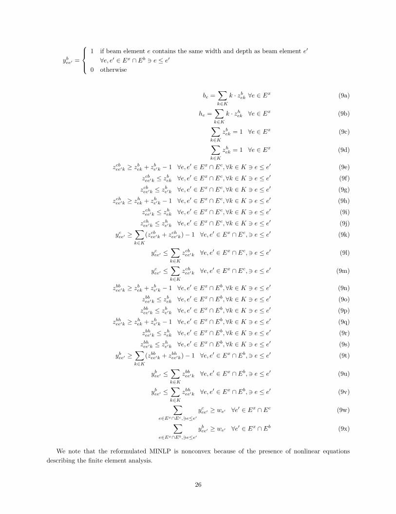
ybee′ =

1 if beam element e contains the same width and depth as beam element e′

∀e, e′ ∈ Ex ∩ Eb ∋ e ≤ e′

0 otherwise

be =∑

k∈K

k · zbek ∀e ∈ Ex (9a)

he =∑

k∈K

k · zhek ∀e ∈ Ex (9b)

∑

k∈K

zbek = 1 ∀e ∈ Ex (9c)

∑

k∈K

zhek = 1 ∀e ∈ Ex (9d)

zcbee′k ≥ zbek + zbe′k − 1 ∀e, e′ ∈ Ex ∩ Ec, ∀k ∈ K ∋ e ≤ e′ (9e)

zcbee′k ≤ zbek ∀e, e′ ∈ Ex ∩ Ec, ∀k ∈ K ∋ e ≤ e′ (9f)

zcbee′k ≤ zbe′k ∀e, e′ ∈ Ex ∩ Ec, ∀k ∈ K ∋ e ≤ e′ (9g)

zchee′k ≥ zhek + zhe′k − 1 ∀e, e′ ∈ Ex ∩ Ec, ∀k ∈ K ∋ e ≤ e′ (9h)

zchee′k ≤ zhek ∀e, e′ ∈ Ex ∩ Ec, ∀k ∈ K ∋ e ≤ e′ (9i)

zchee′k ≤ zhe′k ∀e, e′ ∈ Ex ∩ Ec, ∀k ∈ K ∋ e ≤ e′ (9j)

ycee′ ≥∑

k∈K

(zcbee′k + zchee′k)− 1 ∀e, e′ ∈ Ex ∩ Ec,∋ e ≤ e′ (9k)

ycee′ ≤∑

k∈K

zcbee′k ∀e, e′ ∈ Ex ∩ Ec,∋ e ≤ e′ (9l)

ycee′ ≤∑

k∈K

zchee′k ∀e, e′ ∈ Ex ∩ Ec,∋ e ≤ e′ (9m)

zbbee′k ≥ zbek + zbe′k − 1 ∀e, e′ ∈ Ex ∩ Eb, ∀k ∈ K ∋ e ≤ e′ (9n)

zbbee′k ≤ zbek ∀e, e′ ∈ Ex ∩ Eb, ∀k ∈ K ∋ e ≤ e′ (9o)

zbbee′k ≤ zbe′k ∀e, e′ ∈ Ex ∩ Eb, ∀k ∈ K ∋ e ≤ e′ (9p)

zbhee′k ≥ zhek + zhe′k − 1 ∀e, e′ ∈ Ex ∩ Eb, ∀k ∈ K ∋ e ≤ e′ (9q)

zbhee′k ≤ zhek ∀e, e′ ∈ Ex ∩ Eb, ∀k ∈ K ∋ e ≤ e′ (9r)

zbhee′k ≤ zhe′k ∀e, e′ ∈ Ex ∩ Eb, ∀k ∈ K ∋ e ≤ e′ (9s)

ybee′ ≥∑

k∈K

(zbbee′k + zbhee′k)− 1 ∀e, e′ ∈ Ex ∩ Eb,∋ e ≤ e′ (9t)

ybee′ ≤∑

k∈K

zbbee′k ∀e, e′ ∈ Ex ∩ Eb,∋ e ≤ e′ (9u)

ybee′ ≤∑

k∈K

zbhee′k ∀e, e′ ∈ Ex ∩ Eb,∋ e ≤ e′ (9v)

∑

e∈Ex∩Ec,∋e≤e′

ycee′ ≥ we′ ∀e′ ∈ Ex ∩ Ec (9w)

∑

e∈Ex∩Eb,∋e≤e′

ybee′ ≥ we′ ∀e′ ∈ Ex ∩ Eb (9x)

We note that the reformulated MINLP is nonconvex because of the presence of nonlinear equations

describing the finite element analysis.

26

References

Abramson M.A. (2006, May). Air Force Institute of Technology, Retrieved from

http://www.afit.edu/en/enc/Faculty/MAbramson/nomadm.html

Abramson, M.A. (2005). “Second Order Behavior of Pattern Search,” SIAM Journal on Optimization.

16(2): 315-330.

American Concrete Institute (ACI). (2005). Committee 318 Building Code Requirements for Structural

Concrete (ACI 318-05) and Commentary (ACI 318R-05), Detroit.

AMPL Optimization LLC. (2001). AMPL Version 10.6.16. www.ampl.com.

Balling, R.J. (2002). “Decomposition Methods in Structural Optimization,” in ASCE Recent Advances

in Optimal Structural Design, Burns, S.A., editor. 41-53. New York.

Balling, R.J., and Yao, X. (1997). “Optimization of Reinforced Concrete Frames,” J. of Structural

Engineering, ASCE. 123(2): 193-202.

Bussieck, M.R., and Pruessner, A. (2003). “Mixed-Integer Nonlinear Programming,” GAMS Develop-

ment Corporation.

Camp, C.V., Pezeshk, S., and Hansson, H. (2003). “Flexural Design of Reinforced Concrete Frames

using a Genetic Algorithm,” Journal of Structural Engineering. 129(1): 105.

Corradi, L., De Donato, O., and Maier, G. (1974). “Inelastic Analysis of Reinforced Concrete Frames,

Journal of the Structural Division,” J. of the Structural Division, ASCE. 100(9): 1925-1942.

De Donato, O., and Maier, G. (1972). “Mathematical Programming Methods for the Inelastic Analysis

of Reinforced Concrete Frames Allowing for Limited Rotation Capacity,” Int. J. Num. Meth. Engng.

4: 307-329.

Dinno K.S., and Mekha, B.B. (1993). “Optimal Design of Reinforced Concrete Frames Based on

Inelastic Analysis,” Computers and Structures. 47(2): 245-252.

Dinno K.S., Mekha, B.B. (1995). “A Developed Algorithm for the Inelastic Analysis of Reinforced

Concrete Frames,” Computers and Structures. 57(2): 227-232.

Duran M., and Grossman, I.E. (1986). “An Outer-Approximation Algorithm for a Class of Mixed

Integer Nonlinear Programs,” Mathematical Programming 36: 307.

Fadaee, M.J., and Grierson, D.E. (1996). “Design Optimization of 3D Reinforced Concrete Structures,”

Structural Optimization, Springer-Verlag. 12(1-2): 127-134.

Ferris, M.C., and Tin-Loi, F. (1999). “On the Solution of a Minimum Weight Elastoplastic Problem

Involving Displacement and Complementarity Constraints,” Computer Methods in Applied Mechanics

and Engineering. 174: 107-120.

Fletcher, R., and Leyffer, S. (2004). “Solving Mathematical Program with Complementarity Con-

straints as Nonlinear Programs,” Optimization Methods and Software, 19(1): 15-40.

Fletcher, R., and Leyffer, S. (1998). User Manual for filterSQP. Numerical Analysis Report NA/181,

Dundee University, Dundee, Scotland.

27

Fourer, R., Gay D., and Kernighan, B. (2003). AMPL A Modeling Language for Mathematical Programming,

Thompson Learning, Pacific Grove, CA.

Geoffrion, A.M. (1972). “Generalized Benders Decomposition,” Journal of Optimization Theory and

Applications 10: 237-260.

Guerra, A., and Kiousis P.D. (2006). “Design Optimization of Reinforced Concrete Structures,” Com-

puters and Concrete. 3(5): 313.

Guerra, A. (2008). “Design of Reinforced Concrete Using Mixed Integer Nonlinear Programming,”

Ph.D. Dissertation. Colorado School of Mines, Golden CO.

Horowitz, B., and Moraes, G.R. (2005). “Mathematical Programming with Complementarity Con-

straints Applied to Limited Ductility Analysis of Concrete Beams,” 6th World Congresses of Structural

and Multidisciplinary Optimization. Rio De Janeiro, Brazil.

Inel, M., and Ozmen, H.B. (2006). “Effects of Plastic Hinge Properties in Nonlinear Analysis of

Reinforced Concrete Buildings,” Engineering Structures. 28: 1494-1502.

Kaneko, I. (1977). “A Mathematical Programming Method for the Inleastic Analysis of Reinforced

Concrete Frames,” International J. for Numerical Methods in Engineering, Wiley and Sons. 11: 1137.

Krishnamoorthy, C.S., and Mosi, D.R. (1981). “Optimal Design of Reinforced Concrete Frames Based

on Inelastic Analysis,” Engineering Optimization. 5: 151-167.

Lee, C., and Ahn, J. (2003). “Flexural Design of Reinforced Concrete Frames by Genetic Algorithm,”

Journal of Structural Engineering. 129(6): 762.

Leyffer, S. (1999). User Manual for MINLPBB, University of Dundee Numerical Analysis Report

NA/XXX. Dundee University, Dundee, Scotland.

Leyffer, S. (2001). “Integrating SQP and Branch-and-Bound for Mixed Integer Nonlinear Program-

ming,” Computational Optimization and Applications. 18: 295-309.

Maier, G., Giannessi, F., and Nappi, A. (1982). “Indirect Identification of Yield Limits by Mathemat-

ical Programming,” Engineering Structures. 4: 86-98.

Scheel, H., and Scholtes, S. (2000). “Mathematical Programs with Complementarity Constraints:

Stationarity, Optimality, and Sensitivity,” Mathematics of Operations Research. 25(1): 1-22.

Sahinidis, N.V. (2006). Private communication.

SEI/ASCE 7-98. (2000). Minimum Design Loads for Buildings and Other Structures, American Society

of Civil Engineers, Reston, VA.

Tawarmalani, M., and Sahinidis, N.V. (2002). “Convexification and Global Optimization in Contin-

uous and Mixed-Integer Nonlinear Programming: Theory, Algorithms, Software, and Applications,

Nonconvex Optimization and its Applications series,” Kluwer Academic Publishers. Boston MA. 65.

Torczon, V. (1997). “On the Convergence of Pattern Search Algorithms,” SIAM Journal on Opti-

mization. 7(1): 1-25.

28

The submitted manuscript has been created by the UChicago Argonne, LLC, Operator of Argonne National Laboratory (“Argonne”)

under Contract No. DE-AC02-06CH11357 with the U.S. Department of Energy. The U.S. Government retains for itself, and others

acting on its behalf, a paid-up, nonexclusive, irrevocable worldwide license in said article to reproduce, prepare derivative works,

distribute copies to the public, and perform publicly and display publicly, by or on behalf of the Government.

29