Concept Hierarchy in Data Mining: Specificat ion, Generat ion and ... · Data mining is the...
117
Concept Hierarchy in Data Mining: Specificat ion, Generat ion and Implement at ion Yijun Lu M.Sc., Simon Fraser University, Canada, 1995 B.Sc., Huazhong University of Science and Technology, China, 1985 A THESIS SUBMITTED IN PARTIAL FULFILLMENT OF THE REQUIREMENTS FOR THE DEGREE OF MASTER OF SCIENCE in the School of Computing Science @ Yijun Lu 1997 SIMON FRASER UNIVERSITY December 1997 All rights reserved. This work may not be reproduced in whole or in part, by photocopy or other means, without the permission of the author
Transcript of Concept Hierarchy in Data Mining: Specificat ion, Generat ion and ... · Data mining is the...

Concept Hierarchy in Data Mining: Specificat ion, Generat ion and Implement at ion
Yijun Lu
M.Sc., Simon Fraser University, Canada, 1995
B.Sc., Huazhong University of Science and Technology, China, 1985
A THESIS SUBMITTED I N PARTIAL FULFILLMENT
OF T H E REQUIREMENTS FOR T H E DEGREE O F
MASTER OF SCIENCE in the School
of
Computing Science
@ Yijun Lu 1997
SIMON FRASER UNIVERSITY
December 1997
All rights reserved. This work may not be
reproduced in whole or in part, by photocopy
or other means, without the permission of the author

National Library Bibli-ue nationale du Canada
A~quisitions and Acquisitions et '
Bibliographic Services services bibliographiques
395 Wellington Street 395, rue Wellington OnawaON KlAON4 OnawaON K l A O N 4 Canada Canada
The author has granted a non- exclusive licence allowing the National Library of Canada to reproduce, loan, distribute or sell copies of h s thesis in microform, paper or electronic formats.
The author retains ownership of the copyright in hs.thesis. Neither the thesis nor substantial extracts from it may be printed or otherwise reproduced without the author's
Your fib Vorre ~ k r s n c a
Our hle Nofre reference
L'autelir a accorde une licence non exclusive permettant a la Bibliotheque nationale du Canada de reproduire, prEter, distribuer ou vendre des copies de cette these sous la forme de microfiche/film, de reproduction sur papier ou sur format electronique.
L'auteur conserve la propriete du droit d'auteur qui protege cette these. Ni la these ni des extraits substantiels de celle-ci ne doivent &re imprimes ou autrement reproduits sans son autorisation.

APPROVAL
Name:
Degree: \ las ter of Science
Title of thesis: Concept Hierarchy in D a t a >lining: Specification. Gen-
erat ion and b Implementation
Examining Committee: Dr. Hassan :lit-Kaci
('hair
Dr. Jiakvei Han
Senior Sulwrvisor
-
Dr . \'eronica Dahl
Supervisor
Dr. Qiang l .ang
Estvrnal Esariiincr
-- \)pi I & , 1'1'17 Date Approved: l
.

Abstract
Data mining is the nontrivial extraction of implicit, previously unknown, and po-
tentially useful information from data. As one of the most important background
knowledge, concept hierarchy plays a fundamentally important role in data mining.
It is the purpose of this thesis to study some aspects of concept hierarchy such as the
automatic generation and encoding technique in the context of data mining.
After the discussion on the basic terminology and categorization, automatic gen-
eration of concept hierarchies is studied for both nominal and numerical hierarchies.
One algorithm is designed for determining the partial order on a given set of nominal
attributes. The resulting partial order is a useful guide for users to finalize the concept
hierarchy for their particular data mining tasks. Based on hierarchical and partition-
ing clustering methods, two algorithms are proposed for the automatic generation of
numerical hierarchies. The quality and performance comparisons indicates that the
proposed algorithms can correctly capture the distribution nature of the concerned
numerical data and generate reasonable concept hierarchies. The applicability of the
algorithms is also discussed and some useful guides are given for the selection of the
algorithms. As an important technique for efficient implementation, encoding of con-
cept hierarchy is investigated. An encoding method is presented and its properties are
studies. The superior advantages of this method are shown by comparing the storage
requirement and performance with some other techniques. Finally, the applications
of concept hierarchies in processing typical data mining tasks are discussed.

Acknowledgments
I would like to express my deepest gratitude to my senior supervisor, Dr.Jiawei Han.
He has provided me with inspiration both professionally and personally during the
course of my degree. The completion of this thesis would not have been possible
without his encouragement, patient guidance and constant support.
I am very grateful to Dr.Veronica Dahl for being my supervisory committee mem-
ber and Dr.Qiang Yang for being my external examiner. They were generous with
their time to read this thesis carefully and make thoughtful suggestions.
My thanks also go to Dr.Yongjian Fu for his valuable suggestions and comments,
and to my fellow students and colleagues in the Database Systems Laboratory, Jenny
Chiang, Sonny Chee, Micheline Kamber, Betty Xia, Cheng Shan, Wan Gong, Nebojsa
Stefanovic, and Kris Koperski for their assistance and friendship.
Financial supports from the research grants of Dr.Jiawei Han and from the School
of Computing Science at Simon Fraser University are much appreciated.
Finally, my special thanks are due to my wife, Ying Zhang, for her love and care
these years.

Contents
... . . . . . . . . . . . . . . . . . . . . . . . . . . . . . . . . . . . . . Abstract 111
. . . . . . . . . . . . . . . . . . . . . . . . . . . . . . . . Acknowledgments iv ... . . . . . . . . . . . . . . . . . . . . . . . . . . . . . . . . . . List of Tables v11l
. . . . . . . . . . . . . . . . . . . . . . . . . . . . . . . . . . List of Figures ix
1 Introduction . . . . . . . . . . . . . . . . . . . . . . . . . . . . . . . 1
. . . . . . . . . . . . . 1.1 Data Mining and Knowledge Discovery 3
. . . . . . . . F1.2 The Role of Concept Hierarchy in Data Mining 4
. . . . . . . . . . . . . . . . . . . . . . . . . . . . . 1.3 Motivation 6
1.4 Outline of the Thesis . . . . . . . . . . . . . . . . . . . . . . . 7
. . . . . . . . . . . . . . . . . . . . . . . . . . . . . . . 2 Related Work 9
. . . . . . . . . . . . 2.1 Concept Hierarchy in Data Warehousing 9
. . . . . . . . . . . . . . . / . 2.2 Concept Hierarchy in Data Mining 11
. . . . . . . . . . . . . . . . 2.3 Concept Hierarchy in Other Areas 12
. . . . . . . . . . . . . . . . . . . . . . . . . . . . . 2.4 Summary 14
. . . . . . . . . . . . . . . . . . . 3 Specification of Concept Hierarchies 15
. . . . . . . . . . . . . . . . . . . . . . . . . . . 3.1 Preliminaries 15
. . . . 3.2 A Portion of DMQL for Specifying Concept Hierarchies 22
. . . . . . . . . . . . . . . . . . 3.3 Types of Concept Hierarchies 23

. . . . . . . . . . . . . . . . . . . . 3.3.1 Schema hierarchy 23
. . . . . . . . . . . . . . . . . 3.3.2 Set-grouping hierarchy 25
. . . . . . . . . . . . . . 3.3.3 Operation-derived hierarchy 27
. . . . . . . . . . . . . . . . . . 3.3.4 Rule-based hierarchy 28
. . . . . . . . . . . . . . . . . . . . . . . . . . . . . 3.4 Summary 32
. . . . . . . . . . . . . 4 Automatic Generation of Concept Hierarchies 33
. . . . . . . . . . 4.1 Automatic Generation of Nominal Hierarchies 34
4.1.1 Algorithm . . . . . . . . . . . . . . . . . . . . . . . . 34
. . . . . . . . . . . . . . . 4.1.2 On date/time Hierarchies 37
. . . . . . . . 4.2 Automatic Generation of Numerical Hierarchies 38
. . . . . . . . . . . . . . . . . . . . 4.2.1 Basic Algorithm 39
. . . . . 4.2.2 An Algorithm Using Hierarchical Clustering 41
. . . . . 4.2.3 An Algorithm Using Partitioning Clustering 46
. . . . . . . . 4.2.4 Quality and Performance Comparison 53
. . . . . . . . . . . . . . . . . . . . . 4.3 Discussion and Summary 59
. . . . . . . . . . . . . . . . . . . . . . 5 Techniques of Implementation 61
. . . . . . . . . . . . . . . . . . . . 5.1 Relational Table Approach 62
. . . . . . . . . . . . . . . . . 5.2 Encoding of Concept Hierarchy 66
. . . . . . . . . . . . . . . . . . . . . . . . 5.2.1 Algorithm 68
. . . . . . . . . . . . . . . . . . . . . . . . 5.2.2 Properties 69
. . . . . . . . . . . . . . . . . . . . . . . . . 5.2.3 Remarks 72
. . . . . . . . . . . . . 5.3 Performance Analysis and Comparison 75
. . . . . . . . . . . . . . . . . . 5.3.1 Storage Requirement 77
. . . . . . . . . . . . . . . . . . . . 5.3.2 Disk Access Time 84
. . . . . . . . . . . . . . . . . . . . . 5.4 Discussion and Summary 87

. . . . . . . . . . . . . . . . 6 Data Mining Using Concept Hierarchies 88
. . . . . . . . . . . . . . . . . . . . . . . . . 6.1 DBMiner System 89
. . . . . . . . . . . . . . . . . . . . . 6.2 DMQL Query Expansion 89
. . . . . . . . . . . . . . . . . . . . . . 6.3 Concept Generalization 91
. . . . . 6.4 On the Utilization of Rule-based Concept Hierarchies 93
. . . . 6.5 Concept Lookup for Displaying Results of Data Mining 94
. . . . . . . . . . . . . . . . . . . . . . . . . . . . . 6.6 Summary 95
. . . . . . . . . . . . . . . . . . . . . . 7 Conclusions and Future Work 96
. . . . . . . . . . . . . . . . . . . . . . . . . . . . . 7.1 Summary 96
. . . . . . . . . . . . . . . . . . . . . . . . . . . . 7.2 Future Work 98
. . . . . . . . . . . . . . . . . . . . . . . . . . . . . . . . . . Bibliography 101
vii

List of Tables
. . . . . . . . . . 4.1 Optimal combination of fan-out and number of bins 58
. . . . . . . . . . . . . . . . . . . . . . . . 5.1 Hierarchy table for location 65
. . . . . . . . . . . . . . . . . . . . . . . 5.2 An date/time hierarchy table 66
. . . . . . . . . . . . . . . . . . . . . . . 5.3 An encoded hierarchy table 74
. . . . . . . . . . . . . . . . . . . . . 5.4 Hierarchy tables for approach A 75
. . . . . . . . . . . . . . . . . . . . . 5.5 Hierarchy tables for approach B 76
* * .
V l l l

List of Figures
3.1 Four sample concept hierarchies . . . . . . . . . . . . . . . . . . . . . .
3.2 A concept hierarchy location for the provinces in Canada . . . . . . . .
3.3 A lattice-like concept hierarchy science . . . . . . . . . . . . . . . . . .
3.4 Top-level DMQL syntax for defining concept hierarchies . . . . . . . .
3.5 A set-grouping hierarchy statusHier for attribute status . . . . . . . .
3.6 A rule-based concept hierarchy gpaHier for attribute GPA . . . . . . .
3.7 Generalization rules for concept hierarchy gpaHier . . . . . . . . . . . .
3.8 A variant of the concept hierarchy gpa Hier . . . . . . . . . . . . . . . .
4.1 A histogram for attribute A . . . . . . . . . . . . . . . . . . . . . . . .
4.2 A concept hierarchy for attribute A generated by algorithm AGH F . . .
4.3 A concept hierarchy for attribute A generated by algorithm AGHC . .
4.4 A concept hierarchy for attribute A generated by Algorithm 4.5 using
WGS (4.1). . . . . . . . . . . . . . . . . . . . . . . . . . . . . . . . .
4.5 A concept hierarchy for attribute A generated by Algorithm 4.5 using
WGS (4.2). . . . . . . . . . . . . . . . . . . . . . . . . . . . . . . . .
4.6 A concept hierarchy for attribute A generated by Algorithm 4.5 using
WGS (4.3). . . . . . . . . . . . . . . . . . . . . . . . . . . . . . . . .
4.7 Another histogram for attribute A . . . . . . . . . . . . . . . . . . . .

4.8 A concept hierarchy for attribute A generated by algorithm AGHC with
input histogram given in Figure 4.7. . . . . . . . . . . . . . . . . . . .
4.9 A concept hierarchy for attribute A generated by algorithm AGPC with
input histogram given in Figure 4.7. . . . . . . . . . . . . . . . . . . .
. . . . . . . . . . 4.10 Comparison of execution time when the fan-out is 3
. . . . . . . . . . 4.11 Comparison of execution time when the fan-out is 5
5.1 Post-order traversal encoding of a small hierarchy . . . . . . . . . . . .
. . . . . . . . . . . . . . . . . . . . . . . 5.2 An encoded concept hierarchy
5.3 Storage comparison for different number of dimensions . . . . . . . . .
5.4 Storage comparison by varying number of levels . . . . . . . . . . . . .
5.5 Storage comparison for different fan-out in hierarchies . . . . . . . . .
5.6 Storage comparison for different concept lengths . . . . . . . . . . . . .
5.7 Storage comparison the number of leaf nodes in hierarchies is fixed . .
5.8 Comparison of disk access time for generalizing a concept . . . . . . .
. . . . . . . . . . . . . . . . . 6.1 Ar~hit~ecture of the DBMiner system
6.2 A sample procedure of code chopping off . . . . . . . . . . . . . .
. . . . . . . . . . . . . . . . . 7.1 A concept hierarchy for attribute age
. . . . . . . . . . . . . 7.2 Another concept hierarchy for attribute age
. . . . . . . . . . . . . . . . . . . . . 7.3 A histogram for attribute age

Chapter 1
Introduction
With the rapid growth in size and number of available databases in commercial,
industrial, administrative and other applications, it is necessary and interesting to
examine how to extract knowledge automatically from huge amount of data.
Knowledge discovery in databases (KDD), or data mining is the nontrivial extrac-
tion of implicit, previously unknown, and potentially useful information from data[l7].
Through the extraction of knowledge in databases, large databases serve as rich, re-
liable sources for knowledge retrieval and verification, and the discovered knowledge
can be applied to information management, decision making, process control and
many other applications. Therefore, data mining has been considered as one of the
most important and challenge research areas. Researchers in many different fields,
including database systems, knowledge-base systems, artificial intelligence, machine
learning, knowledge acquisition, statistics, spatial databases and data visualization,
have shown great interest in data mining. Many industrial companies are approaching
this important area and realize that data mining will provide an opportunity of major
revenue.

C H A P T E R 1 . INTRODUCTION 2
A popular myth about data mining is to expect that a data mining engine (often
called a data miner) will dig out all kinds of knowledge from a database autonomously
and present them to users without humans instructions or intervention. This sounds
appealing. However, as one may aware, an overwhelmingly large set of knowledge,
deep or shallow, from one perspective or another, could be generated from many
different combinations of the sets of the data in the database. The whole set of
knowledge generated from the database, if measured in bytes, could be far large than
the size of the database. Thus it is neither realistic nor desirable t o generate, store,
or present such set of the knowledge discoverable from the database.
A relatively realistic goal is that a user or an expert communicate with a data
miner using a set of data mining primitives for effective and fruitful data mining.
Such primitives include the specification of the portion of a database in which one is
interested, the kind of knowledge or rules to be mined, the background knowledge that
a mining process should use, the desired forms to present the discovered knowledge,
etc.
As one of the useful background knowledge, concept hierarchies organize data or
concepts in hierarchical forms or in certain partial order, which are used for expressing
knowledge in concise, high-level terms, and facilitating mining knowledge at multiple
levels of abstraction. Concept hierarchies are also utilized to form dimensions in
multidimensional databases and thus are essential components for data warehousing
as we11[29].
In this chapter, the tasks of data mining are described in section 1.1, where differ-
ent kinds of rules are introduced. In section 1.2, the role of concept hierarchies in the
basic attribute-oriented induction (AOI) and multiple-level rule mining is discussed.
Motivation of this thesis is addressed in section 1.3. Section 1.4 gives an overview of
the thesis.

C H A P T E R 1. INTRODUCTION
1.1 Data Mining and Knowledge Discovery
There have been many advances on researches and developments of data mining, and
many data mining techniques and systems have recently been developed. Different
philosophical considerations on knowledge discovery in databases may lead to differ-
ent methodologies in the development of KDD techniques. Based on the kinds of
knowledge to be mined, data mining tasks may be classified as follows.
1. Characteristic Rule Mining, the summarization of the general characteristics of a
set of user-specified data in a database. For example, the symptoms of a specific
disease can be summarized by a set of characteristic rules.
2. Discriminant Rule Mining, the discovery of features or properties that distin-
guish one set of data, called target class, from some other set(s) of data, called
contrasting class(es). For example, to distinguish one disease from others, a
discriminant rule summarizes the symptoms that differentiate this disease from
the others.
3. Association Rule Mining, the discovery of association among a set of objects, say,
{A;)z"=,nd {Bj),"=, , in the form of Al A - - . A A, + B1 A . . - A B,. For example,
one may discover that a set of symptoms often occurs together with another set
of symptoms.
4. Classification Rule Mining, the categorization of the data into a set of known
classes. For example, a set of cars associated with many features may be clas-
sified based on their gas mileages.
5. Clustering, the identification of clusters (classes or groups) for a set of objects
based on their attributes. The objects are so clustered that the within-group
similarity is minimized and between-group similarity is maximized based on

C H A P T E R 1 . INTRODUCTION 4
some criteria. For example, a set of diseases can be clustered into several clusters
based on the similarities of their symptoms.
6. Prediction, the forecast of the possible values of some missing data or the dis-
tribution of certain attribute(s) in a set of data. For example, an employee's
salary can be predicted based on the salary distribution of similar employees in
a company.
7. Evolution Rule Mining, the discovery of a set of rules which reflect the general
evolution behavior of a set of data. For example, one may discover the major
factors which influence the fluctuations of certain stock prices.
The data mining tasks described above are part of widely recognized ones. Other data
mining tasks in the form of different knowledge rules have also been studying. Even
for the above stated rules, there exist special forms or variants in different cases. For
example, quantitative association rule mining is the new development of the general
case association rule mining.
1.2 The Role of Concept Hierarchy in Data Min-
ing
Usually, data can be abstracted at different conceptual levels. The raw data in a
database is called at its primit,ive level and the knowledge is said to be at a primitive
level if it is discovered by using raw data only. Knowledge discovery at the primitive
level has been studied extensively. For example, Most of the statistic tools for data
analysis are based on the raw data in a data set.
Abstracting raw data to a higher conceptual level, and discovering and expressing

C H A P T E R 1 . INTRODUCTION 5
knowledge at higher abstraction levels have superior advantages over data mining at
a primitive level. For example, if we have discovered a rule at a primitive level as
follows.
Rule 1: 80% of peoples who are titled as professor, senior engineer,
doctor and lawyer are have salary between $60,000 and $1 00,000.
After abstracting data to certain higher levels, we may have the following rule.
Rule 2: General speaking, well educated people get well paid.
Obviously, Rule 2 is much conciser than Rule 1, and, to certain extent, convey more
information. What we have done here is to abstract people titled with professor, senior
engineer, doctor and lawer to a higher conceptual level, i.e., well educated people. And
we generalize salary between $60,000 and $100,000 to higher level concept well paid.
Different sets of data could have different abstractions and then organized to form
different concept hierarchies. A formal definition of concept hierarchy will be given
in 53.1.
Concept hierarchies can be used in the processing of all the tasks stated in the last
section. For a typical data mining task, the following basic steps should be executed
and concept hierarchies play a key role in these steps.
1. Retrieval o f t he task-related data set. Generation of a data cube.
2. Generalization o f raw data t o certain higher abstraction level.
3. Further generalization or specialization. Multiple-level rule mining.
4. Display o f discovered knowledge.

CHAPTER 1. INTRODUCTION
Before proceeding to the next section, It is worth pointing out that concept hi-
erarchies also have the fundamental importance in data warehousing techniques. In
a typical data warehousing system, dimensions are organized in the form of concept
hierarchies. Therefore, the OLAP operations roll-up and drill-down can be performed
by concept (or data) generalization and specialization.
Motivation
The incoperation of concept hierarchies into data mining and data warehousing tech-
niques has produced many important research results as well as useful systems. How-
ever most of the effort in research and industry has been put on the utilization of
concept hierarchies. Of course, it is the ultimate goal of all the studies on concept
hierarchies. However, their efficient use should be based upon the complete under-
standing of different aspects and techniques concerning concept hierarchies. Some of
the problems related to concept hierarchies are listed as follows.
1. Basic terminology is necessary for unifying the study on concept hierarchies.
2. Different attributes in a database may be of different types, and concept hier-
archies for those attributes may also have different types. Thus, what possible
types of concept hierarchies can we have and what are their properties? How
do we specifiy or define those concept hierarchies?
3. Construct a large concept hierarchy is tedious and very time-consurmming even
for a domain expert. Can we generate concept hierarchies automatically? How
do we design generation algorithms and how to use those algorithms?
4. In our mind a concept hierarchy may have a layered structure, in a data mining
system, however, how to store a,nd manipulate it? How to provide a machinisim

CHAPTER 1. INTRODUCTION
to concept hierarchies to realize efficient use in data mining?
These and other problems let us recognize the fundamental importance of concept
hierarchies and motivate us to conduct an indepth study on concept hierarchy. The
concept hierarchies may be applied to other areas and may have other problems, but
we confine our study in the context of data mining and data warehousing.
Outline of the Thesis
The remainder of the thesis is organized as follows. In Chapter 2, a brief survey of the
related work on concept hierarchies is given. Some interesting problems concerning
concept hierarchies are also stated there.
In Chapter 3, the preliminaries of concept hierarchy such as its formal definition,
properties, classification, language specification a,nd basic terminology are described
and discussed. These will serve as the base of our study in latter chapters.
In Chapter 4, we focus on the automatic generation of concept hierarchies for
nominal and numerical attributes. The algorithm presented there for the automatic
generation of schema hierarchies is based on the statistics of data in a relation. The
two algorithms proposed for automatic generation of numerical hierarchies are based
on clustering methods with order constraints. Both hierarchical and partitioning clus-
tering techniques are utilized as components in our design of generation algorithms.
The quality and performance comparison of the algorithms gives a guidance for the
selection of different algorithms.
Chapter 5 discusses the techniques for efficient implementation of concept hier-
archies in our new version of DBMiner system. The relational table approach is

C H A P T E R 1. INTRODUCTION
addressed with a comparison with the traditional file operating approach. The en-
coding technique of concept hierarchies and its application substantially improve the
performance of our data mining system. An algorithm is developed for the purpose of
hierarchy encoding. The performance comparison of the employment of encoded hier-
archies against non-encoded ones conducted there shows the evendence of the superior
of our encoding technique.
Chapter 6 considers the application of concept hierarchies in the typical data
mining system, DBMiner. Where we will discuss how to utilize concept hierarchies in
DMQL query processing, concept generalization, handling information loss problems
in use of rule-based hierarchies and display of finial mining results.
Finally, we summarize the thesis in Chapter 7, in which some interesting problems
are addressed for future study.

Chapter 2
Related Work
In the early studies or in areas other than data mining, concept hierarchy is commonly
called taxonomy. We adopt the term concept hierarchy because of the popularity of
this term in the community of data mining and knowledge discovery.
In this chapter, we briefly go through the previous work related to concept hier-
archy in the context of data warehousing, data mining and some other areas.
Concept Hierarchy in Data Warehousing
While operational databases maintain state information, data warehouses typically
maintain historical information. Although there are several forms of schema, e.g.,
star schema and snowflake schema, in the design of a data warehouse, the fact tables
and dimension tables are its essential components. Users typically view the fact tables
as multidimensional data cubes. Usually the attributes of a dimension table may be
organized as one or more concept hierarchies.

CHAPTER 2. RELATED WORK 10
The use of concept hierarchies in a data warehousing system provides the foun-
dation of operations roll-up and drill-down. Harinarayan, Rajaraman and Ullman[29]
studied the view materialization problem when hierarchical dimensions are involved
in the construction of data cubes. To improve the performance of executing OLAP
operations, a lattice framework is used to express dependencies among views. These
dependencies are actually introduced by using concept hierarchies. A more recent re-
search by Wang and Iyer[49] proposed an encoding method of concept hierarchies for
benefiting the roll-up and drill-down queries of OLAP. The post-order labeling method
used in [49] demonstrates better performance than the traditional join method in the
DB2 V2 system. Different from other researches, this work focuses on the topic of how
to efficiently use concept hierarchies to improve the performance of OLAP queries.
Many commercial products of OLAP systems are available, and Cognos PowerPlay
[42], Oracle Express[S] and Microstrategy DSS[11] are among the most popular ones.
Since the analysis of historical information for decision support is the ultimate goal
of any data warehousing systems, at least one time dimension should be involved in
the construction of data cubes. Once the time period is specified, a time dimension
is reasonably stable. The flexibility of time schema lets PowerPlay, Express and DSS
put a great deal of effort to handle different time dimensions. One interesting thing is
that, usually numerical attributes are taken as measurements and thus assigned as a
measure or fact in the fact tables. Of course, one can take attribute age as a measure-
ment and obtain some aggregates such as avg(age) over a set of data. However, when
we compare attributes accou nt-balance with age we can find that account-bala nce has
more meaning of measurement. It could be more useful to build a concept hierarchy
for age and place attribute age in a dimension table. The vacancy of the generation
of concept hierarchies for numerical attributes is the common disadvantage of the
current commercial OLAP products.

CHAPTER 2. RELATED WORK
Concept Hierarchy in Data Mining
The formal use of concept hierarchies as the most important background knowledge
in data mining is introduced by Han, Cai and Cercone[24]. The incorporation of
concept hierarchy into the attribute-oriented induction (AOI) leads A01 to be one
of the most successful techniques in data mining. Concept hierarchies have been
used in various algorithms such as characteristic rule mining[24] [27], multiple-level
association mining[26], classification[31] and prediction.
Association rule and its initial mining algorithm is proposed by Agrawal, Imielinski
and Swami[2] and fast algorithms are reported in Agrawal and Srikant [3]. However,
they do not consider any concept generalization and only discover patterns using
raw data, in other words, the discovered knowledge is solely at the primitive level.
Upon recognizing the importance of concept hierarchies, they proposed algorithms
for mining generalized association rules in Srikant and Agrawal[46], in which concept
hierarchies are used for mining association rules and interesting rule detections. In-
terestingness is an important measure to determine the value of the discovered knowl-
edge. In [21], the complexity of a concept hierarchy is defined in terms of the number
of its interior nodes, and the depth and height of each of these interior node. This
complexity is then used to measure the interestingness of the discovered knowledge
rules.
In the term of structured attributes, Michalski, e t a1 [39, 331 studied the discovery of
generalization rules using concept hierarchies. For numerical attributes, a generation
method called ChiMerge is employed. ChiMerge is proposed by Kerber[36] in order
to discretize numerical attributes such that classification could be done with higher
accuracy. ChiMerge is designed solely for classification in which several classification
attributes must be pre-specified. Otherwise, the X 2 value is impossible to be obtained

CHAPTER 2. RELATED WORK
if there is no any classification attributes given.
In 1994, Han and Fu[25] reported a study on the automatic generation and dynamic
adjustment of concept hierarchies based on data mining tasks. The role of concept
hierarchies in the attribute-oriented induction is clarified and several algorithms are
developed for the generation and adjustment of concept hierarchies.
The term rule-based concept hierarchy is first used in Cheung, Fu and Han[7] for
the purpose of extending generalization of concepts from unconditional to conditional.
Some difficulties are discussed in using rule-based concept hierarchies and an algorithm
is presented to solve the problems and to complete the AOI procedure.
Date mining and data warehousing are not the two totally independent fields.
Actually, when we look at their internal architectures, we find that they are essen-
tially built on the same data source called data cube. One can take data mining as
an extension of data warehousing by adding many more powerful functionalities or
functional modules for discovering more types of knowledge rules. In this sense, we do
not differentiate the techniques, especially those for concept hierarchies, used in data
mining and data warehousing. As a matter of fact, the integration of the function-
alities of data warehousing and data mining has been implemented in our DBMiner
system. Refer to Han[23] for more details on this issue.
Concept Hierarchy in Other Areas
Concept hierarchies have long been used in other areas in the name of taxonomies. As
a matter of fact, many important research results on data mining are from machine
learning and statistics, etc. Concept hierarchies play an important role in knowledge
representation and reasoning[38, 51. As the size of concept hierarchies increases, there

CHAPTER 2. RELATED WORK
is a growing need to represent them in a form that is amenable to performing op-
erations efficiently. Encoding hierarchies in a manner that permits quick execution
of such operations has been a goal in logic programming and other areas of com-
puter science[l4]. Many encoding schemes have been proposed such as in Dahl[9, 101,
Brew[5] and Ai't-Kaci, e t a1 [4]. Although those encoding schemes are successful in
their particular fields, research is ongoing in the quest for general purpose, compact,
flexible and efficient encoding techniques.
Interesting studies on the automatic generation of concept hierarchies for nominal
data can also be seen in other areas, which can be categorized into different ap-
proaches: machine learning approaches[40, 151, statistical approaches[2], visual feed-
back approaches[35], and algebraic (lattice) approaches[41].
Machine learning approach for concept hierarchy generation is a problem closely
related to concept formation. Many influential studies have been performed on i t ,
including Cluster/2 by Nlichalski and Stepp[40], COBWEB by Fisher[l5], hierarchical
and parallel clustering by Hong and Ma[30].
As a fundamental component in the automatic generation of concept hierarchies
which will be discussed in Chapter 4 of this thesis, data clustering techniques have
been used in many field such as biology, social science, planning and image processing
(see [43]). Although its statistical background is not that strict, numerous researches
on clustering have been conducted since Sokal and Sneath[45] introduced methods for
numerical taxonomy which made a big progress from subjectivity to objectivity. Clus-
ter analysis is highly empirical. Different methods can lead to different grouping[l].
Furthermore, since the groups are not known a priori, it is usually difficult to judge
whether the results make sense in the context of the problem being studied. That is
also the reason we reconsider the particular clustering methods when order constraints
are involved in the automatic generation of numerical hierarchies.

CHAPTER 2. RELATED W O R K
2.4 Summary
Some related work on the research of concept hierarchy in the context of data ware-
housing, data mining and some other areas such as machine learning, statistics, plan-
ning and image processing are summarized. A great deal of those researches is con-
cerning the utilization of concept hierarchies in different algorithms. The research
work on the generation and techniques for efficient implementation of concept hierar-
chy is relatively little. These are the major topics of the thesis and will be studied in
the rest chapters of the thesis.

Chapter 3
Specificat ion of Concept
Hierarchies
The importance of concept hierarchies stimulate us to conduct a systematic study on
them. In this Chapter, we give a formal definition of concept hierarchy, and study
its properties in section 3.1. Some basic terms such as nearest ancestor, level name,
schema level partial order are introduced. In section 3.2, the portion of DMQL for
specifying concept hierarchies is described. In section 3.3, concept hierarchies are
categorized into four types based on t,he methods of specifying them. Finally, we
summarize this chapter in section 3.4.
3.1 Preliminaries
The definition of concept hierarchy is introduced in this section. Some basic terms
are also discussed.
In traditional philosophy, a concept is determined by its extent and intent, where
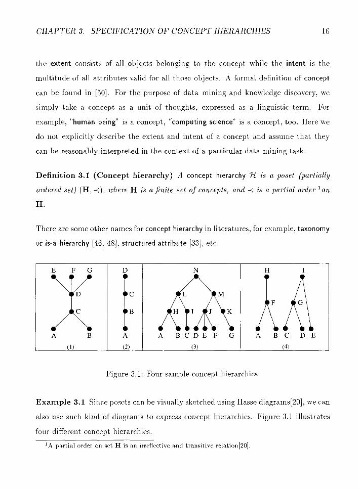
CHAPTER 3. SPECIFICATION OF CONCEPT HIERARCHIES 16
the extent consists of all objects belonging to the concept while the intent is the
multitude of all attributes valid for all those objects. A formal definition of concept
can be found in [50]. For the purpose of data mining and knowledge discovery, we
simply take a concept as a unit of thoughts, expressed as a linguistic term. For
example, "human being" is a concept, "computing science" is a concept, too. Here we
do not explicitly describe the extent and intent of a concept and assume that they
can be reasonably interpreted in the context of a particular data mining task.
Definition 3.1 (Concept hierarchy) A concept hierarchy 'FI is a poset (partially
ordered set) ( H , +), where H is a finite set of concepts, and + is a partial order ' o n
H .
There are some other names for concept hierarchy in literatures, for example, taxonomy
or is-a hierarchy [46, 481, structured at t r ibute [33], etc.
A B C D E F G
Figure 3.1 : Four sample concept hierarchies.
Example 3.1 Since posets can be visually sketched using Hasse diagrams[20], we can
also use such kind of diagrams to express concept hierarchies. Figure 3.1 illustra.tes
four different concept hierarchies.
'A partial order on set H is an irreflective and transitive relation[20].

CHAPTER 3. SPEClFlCATION OF CONCEPT HIERARCHIES 17
Definition 3.2 (Nearest ancestor) A concept y is called the nearest ancestor of
concept x if x, y E H with x -4 y , x # y, and there i s no other concept z E H such
that x 4 z and z 4 y .
Definition 3.3 (Regular concept hierarchy) A concept hierarchy 'FI = (H, 4) is
regular if there is a greatest element in H and there are sets H l , 1 = 0,1, ..., (n - 1))
such that n-1
H = U Hl and H i n H j = 0 for z # j , 1=0
and, if a nearest ancestor of a concept in Hi is in H j , then the nearest ancestors of
the other concepts in Hi are all in H j
Example 3.2 Following definition 3.3, we find that concept hierarchies (2) and (3)
in Figure 3.1 are regular concept hierarchies. For concept hierarchy (3) , the greatest
element is N and we have Ho = {N), H1 = { L , M ) , H2 = { H , I , J, I<) and H3 =
{ A , B , C , D, E , F, (3.
From now on, we will focus our discussions on regular concept hierarchies and call
regular concept hierarchy as concept hierarchy or, simply, hierarchy.
Usually, the partial order 4 in a concept hierarchy reflects the special-general
relationship between concepts, which is also called subconcept-superconcept relation
(see [50, 471). Another important term for describing the degree of generality of
concepts is level number. We assign zero as the level number of the greatest element
(called most general concept) of H, and the level number for each of the other concepts
is one plus its nearest ancestor's level number. A concept with level number 1 is also
called a concept a t level 1.
Due to the layered structure of a hierarchy as described in definition 3.3, we notice
that all the concepts with the same level number must be in set Hr for one and only
one I , 1 = 0 , . . . , (n - 1). We thus simply call Hl as level 1 of the concept hierarchy.

CHAPTER 3. SPECIFICATION OF CONCEPT HIERARCHIES
Now, let us define function g : H + H as
x i f x e H o , g(x) =
y if y is a nearest ancestor of x.
If we impose a constraint that function g is single valued, that is, for any x, y E Hl,
if gl(x) # gr(y) then x # y, then the Hasse diagram of a concept hierarchy is actually
a tree. Therefore, all the terminology for a tree such as node, root, path, leaf, parent,
child, sibling etc. are applicable to the concept hierarchy as well. It is not difficult to
see that g(Hl) C Hl-l for each I = 1,2 , . . . , (n - 1). In the case that g(Hl) = Hl-1 for
each I = 1 ,2 , . . . , (n - l ) , we conclude that every node except the ones in HnP1 has
at least one child.
Definition 3.4 (Level name) A level name is a semantic indicator assigned to a
particular level.
If level numbers are already assigned to the levels of a hierarchy, a simple way to
figure out a level name to each level is to combine word level with its level number.
For example, we assign level2 as the level name of the level with level number 2.
Based on the above discussion, when we talk about a level in a concept hierarchy,
we could use a set of concepts, or the level name assigned to it without any difference.
Example 3.3 A concept hierarchy location for provinces in Canada is shown in Fig-
ure 3.2, which consists of three levels (n = 3) with level names country, region a n d
province, respectively. We have Ho = {Canada), HI = {Western, Central, Mari t ime),
and Hz = {BC, AB, MT, SK, ON, QU, NS, NB, N F , PEI), and relation 4 is defined
as
BC 4 Western 4 Canada:
A B 4 Western 4 Canada;

CHAPTER 3. SPECIFICATION OF CONCEPT HIERARCHlES
Canada country
BC AB MB SK ON Qc NS NB NF PE province
Figure 3.2: A concept hierarchy locat ion for the provinces in Canada.
M B 4 W e s t e r n 4 C a n a d a ;
SIrI 4 W e s t e r n 4 C a n a d a ;
ON 4 C e n t r a l 4 C a n a d a ;
QC 4 C e n t r a l 4 C a n a d a ;
N S 4 M a r i t i m e 4 C a n a d a ;
N B 4 M a r i t i m e 4 C a n a d a ;
N F 3 M a r i t i m e 4 C a n a d a ;
P E 4 M a r i t i m e 4 C a n a d a ;
All the other expressions for this relation, such as BC 4 C a n a d a , ON 4 C a n a d a ,
can be derived from the above expressions using transitivity of the relation. 0
Definition 3.5 (Schema level partial order) A schema level partial order of a con-
cept hierarchy 7-t is a partial order o n S, the set of level names of concept hierarchy
7-t.

CHAPTER 3. SPECIFICATION OF CONCEPT HIERARCHIES 2 0
Let us derive a relation 5 on S from the relation 4 on H as follows: There is a
relation between level names a and b, i.e. a 5 b, if there are two concepts x and y
such that x is in H; whose level name is a , y is in Hj whose level name is b, and a 4 b.
It is not difficult to prove the following
Theorem 3.1 T h e derived relation 5 i s not on ly a partial order o n S, but a total
order as well.
For example, the derived schema level partial order on the set of the level names in
Example 3.3 is
province 4 reg ion 4 c o u n t r y .
On the other hand, if a partial order is given on the set { H 1 } ~ ~ ~ , we can define
a partial order on set Uyzi H1. This is convenient especially when we are concerned
with a relational database, in which HI could be a set of values or instances of an
attribute for each I . A possible relationship between a pair of concepts from different
levels can be naturally created if they belong to the same tuple in a relational table.
Based on this observation, we will use only one notation 4 to denote a partial
order defined for a concept hierarchy regardless of it is defined on the set of concepts
or the set of levels (or level names). Accordingly, a concept hierarchy can be specified
on either schema level or instance level.
Example 3.4 A concept hierarchy da te can be defined as:
d a y 4 m o n t h 4 q u a r t e r 4 year.
This hierarchy is basically regarded as a schema hierarchy which will be discussed
in section 3.3. Here we actually define a schema level partial order from which a
equivalent partial order for the set of the instances of these level names can be derived.

CHAPTER 3. SPECIFICATION OF CONCEPT HlERARCHIES 2 1
For example, the following two expressions demonstrate the application of the partial
order on the set of instances of date values.
Jan.l2,1996 4 January 1996 4 Q1 1996 -i 1996,
Ju1.25,1997 4 Ju ly 1997 4 Q3 1997 4 1997.
In general, functions gl for 1 = 1,2, ..., n can also be multi-valued. In this case, the
concept hierarchy cannot be illustrated as a tree. A lattice-like graph is employed to
visually describe it. More detailed discussion can be seen in 53.3.4 and 56.4.
Example 3.5 A lattice-like hierarchy science is shown in Figure 3.3. where the dis-
cipline data mining has three parents AI , database and statistics.
math & stats physics . . .
A1 . . . database statistics . . . . . . . . .
Figure 3.3: A lattice-like concept hierarchy science.
To ease the latter discussion, we need the following
Definition 3.6 (Root-leaf path) A root-leaf path in a concept hierarchy 'FI is a
path from a node in Ho (called root) to a node in HnW1 (called leaf).

CHAPTER 3. SPECIFICATION OF CONCEPT HIERARCHIES 2 2
3.2 A Portion of DMQL for Specifying Concept
Hierarchies
A data mining query language, DMQL, has been designed and implemented in our
data mining system, DBMiner, for mining several kinds of knowledge in relational
databases at multiple levels of abstraction [28]. It can be employed to specify different
mining tasks such as mining characteristic rules, discriminant rules, association rules,
classification rules and prediction rules. DMQL can also be used for specifying and
manipulating concept hierarchies.
This section describes the portion of DMQL for the specification of hierarchies.
The applications of it will be illustrated using examples in the next section.
The top-level syntax of DMQL for specifying concept hierarchies is shown in Fig-
ure 3.4.
(hierarchy definition) ::= define hierarchy (hierName) [on (relName)] as (hierDef) (hierDef) ::= (attrNameList) [where (condition)]
I (levelsame): (setvalue) (partialorder) (IevelName) : (onevalue) [if (condition)]
I (usingoperation) (attrNameList) ::= (attribute){, (attribute)) (attribute) ::= [(dbName) ..] [(relName) .] (attrName) (set Value) ..- . . - (onevalue) { , (onevalue)) (onevalue) ::= (string) (partialorder) ::= <
Figure 3.4: Top-level DMQL syntax for defining concept hierarchies
The syntax of the DMQL is defined in an extended BNF grammar, where "[ 1" represents 0 or one occurrence, "{ )" represents 0 or more occurrences, and the words

CHAPTER 3. SPECIFICATION OF CONCEPT HIERARCHIES
in sans serif font represent keywords.
3.3 Types of Concept Hierarchies
Concept hierarchies can be categorized into four basic types: schema, set-grouping,
operation-derived and rule-based concept hierarchies. The following subsections give
detailed discussion of these types of concept hierarchies concerning their definitions
and language specifications.
3.3.1 Schema hierarchy
This kind of hierarchy is formed at the schema level by defining the partial order to
reflect relationships among the attributes in a database. For example, the attributes
house-number, street, city, province, and country form a partial order at the schema
level,
house-number 4 street 4 city 4 province 4 country.
For a concrete address, such as "351 Powell street, Vancouver, BC, Canada", its
partial order is determined by the partial order at the schema level for the whole data
relation, and there is no need to specify the generalization or specialization paths for
each record in that data relation.
The following example shows how to use DMQL to define schema hierarchies.
Example 3.6 The home address of the attributes of a relation employee in a company
database is defined in DMQL as follows.
define hierarchy IocationHier on employee as
[house.number, street, city, province, country]

CHAPTER 3. SPECIFICATION OF CONCEPT HIERARCHIES 24
This statement defines the partial order among a sequence of attributes: house-number
is a t one level lower than street, which is in turn at one level lower than city, and so on.
Notice that multiple hierarchies can be formed in a data relation based on different
combinations and orderings of the attributes.
Similarly, a concept hierarchy for date(day, month, quarter, year) is usually pre-
defined by a data mining system, which can be done by using the following DMQL
statement.
define hierarchy timeHier on date as
[day, month, quarter, year]
A concept hierarchy definition may cross several relations. For example, a hier-
archy productHier may involve two relations, product and company, defined by the
following schema.
product (product-id, brand, company, place-made, date-made)
company(name, category, headquarter-location, owner, size, asset, revenue)
The hierarchy productHier is defined in DMQL as follows.
define hierarchy productHier on product, company as
[ p o d u c t i d , brand, product.company, company.category]
where product .company = company.name
In this definition, an attribute name which is shared by two relations has the
corresponding relation name specified in front of the attribute name using the dot
notation as in SQL, and the join condition of the two relations is specified by a where
clause. 0

C H A P T E R 3. SPECIFICATION OF CONCEPT HIERARCHIES 25
An alternative to define a hierarchy involving two or more relations is to define a view
using the relations and where clause, on which the hierarchy is then specified.
Although a hierarchy defined at the schema level determines its partial order and
the generalization and specialization directions, for the purpose of executing a data
mining task, we need to instantiate this schema hierarchy over the related data in a
database to get a concrete or instance hierarchy. The partial orders at both schema
level and instance level should be stored for the purpose of data mining. Some of the
related issues will be discussed in Chapter 5.
3.3.2 Set-grouping hierarchy
This kind of hierarchy is formed by defining set grouping relationships for a set of
concepts (or values of attributes) in order to reflect semantic relationships character-
istic to the given application domain. It is in this sense that Michalski [39] introduced
structured at t r ibute to name this kind of concept hierarchies. A set-grouping hierar-
chy is also called a instance hierarchy because the partial order of the hierarchy are
defined on the set of instances or values of an attribute. We prefer set-grouping to
others because it has more operational sense.
Example 3.7 The concepts freshman, sophomore, junior, senior, undergraduate,
and M.Sc, Ph.D, graduate, which are values of the attribute status in a university
database, form a hierarchy statusHier, such as
{freshman, sophomore, junior, senior) 4 undergraduate
{M.Sc, Ph.D) 4 graduate
{undergraduate, graduate) 4 allstatus

CHAPTER 3. SPECIFICATION OF CONCEPT HIERARCHIES 2 6
Here we use the notation that {Al, A2, ..., Ak) 4 B is equivalent to that A; 4 B for
each i = 1,2, ..., k. This hierarchy can also be visually expressed in Figure 3 .5 .
graduate undergraduate
A M.Sc Ph.D freshman sophomore junior senior
Figure 3.5: A set-grouping hierarchy statusHier for attribute status
The following statement gives the specification of this hierarchy in DMQL.
define hierarchy statusHier as
level2: {freshman, sophomore, junior, senior) < levell: undergraduate;
level2 {M.Sc, Ph.D) < levell: graduate;
levell: {graduate, undergraduate) < level0: allstatus 0
A set-grouping hierarchy can be used for modifying a schema hierarchy or another
set-grouping hierarchy to form a refined hierarchy. For example, one may define a set
grouping relationship within WesternCanada as follows:
{AB, SK, MB) 4 Prairies
{BC, Prairies) 4 WesternCanada
These definitions add a refined layer to the existing definition in the schema hier-
archy location shown in Figure 3.2.
CHAPTER 3. SPECIFICATION OF CONCEPT HIERARCHIES
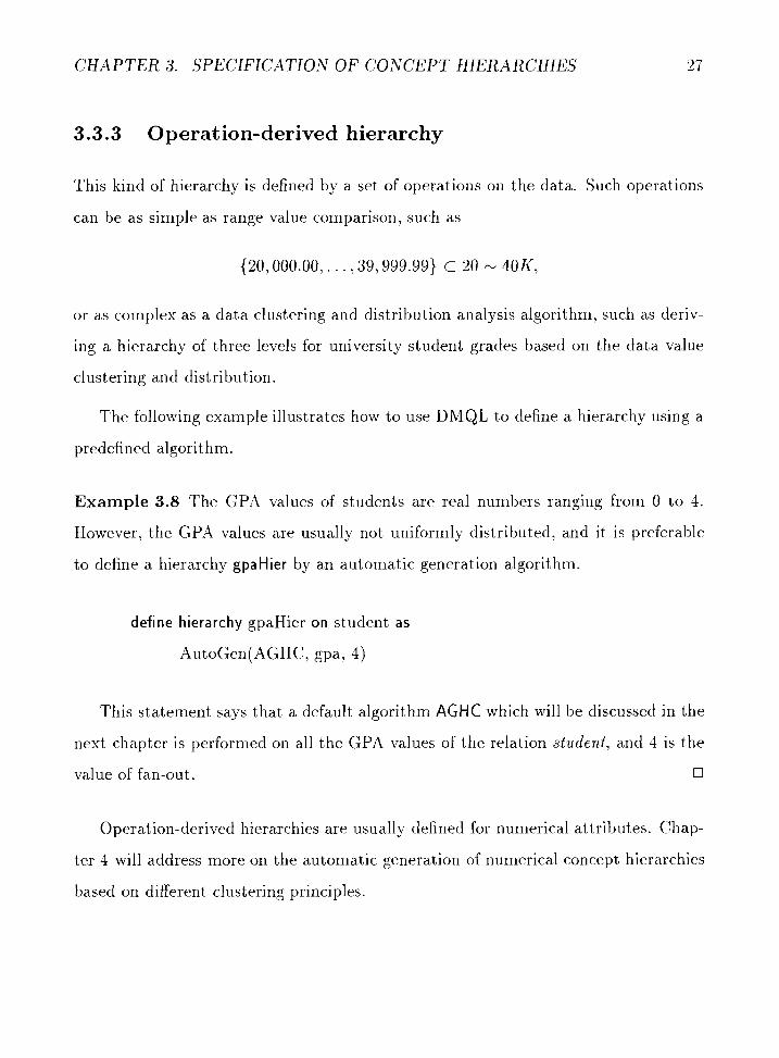
3.3.3 Operation-derived hierarchy
This kind of hierarchy is defined by a set of operations on the data. Such operations
can be as simple as range value comparison, such as
or as complex as a data clustering and distribution analysis algorithm, such as deriv-
ing a hierarchy of three levels for university student grades based on the data value
clustering and distribution.
The following example illustrates how to use DMQL to define a hierarchy using a
predefined algorithm.
Example 3.8 The GPA values of students are real numbers ranging from 0 to 4.
However, the GPA values are usually not uniformly distributed, and it is preferable
to define a hierarchy gpa Hier by an automatic generation algorithm.
define hierarchy gpaHier on student a s
AutoGen(AGHC, gpa, 4)
This statement says that a default algorithm AGHC which will be discussed in the
next chapter is performed on all the GPA values of the relation student, and 4 is the
value of fan-out . 0
Operation-derived hierarchies are usually defined for numerical attributes. Chap-
ter 4 will address more on the automatic generation of numerical concept hierarchies
based on different clustering principles.

CHAPTER 3. SPECIFICATION OF CONCEPT HIERARCHIES
3.3.4 Rule-based hierarchy
The concept hierarchies defined above have the characteristics that, for each concept,
there is only one higher level correspondence, hence a concept can be generalized to
its higher level correspondence unconditionally. For example, in a concept hierar-
chy gpaHier defined for the attribute GPA of database student, a 3.6 GPA (in a 4
points grading system) can be generalized t o a higher level concept, say, excellent.
This concept generalization depends only on the GPA value but not on any other
information of a student. However, in some cases, it may necessary to represent the
background knowledge in such a way that concept generalization would depend not
only on the concept itself but also on other conditions. The same 3.6 GPA may only
deserve a good, if the student is a graduate; and it may be excellent, if the student is
an undergraduate.
A rule-based hierarchy is defined by a set of rules whose evaluation often involves
the data in a database. A lattice-like structure is used for graphically describing this
kind of hierarchies, in which every child-parent path is associated with a generalization
rule.
Example 3.9 Suppose we have a database university, in which a relation student is
defined by the schema student(name, status, sex, major, age, birthplace, GPA). A
rule-based concept hierarchy is shown in Figure 3.6 for its graphical expression and
Figure 3.7 for its generalization rules. Using DMQL, we can define this hierarchy by
statements such as:
define hierarchy gpaHier on student as
level3: "2.0-2.5" < level2: average
i f status = "undergraduate"

CHAPTER 3. SPECIFICATION OF CONCEPT HIERARCHIES
poor average good excellent
R1 Rm 0.0-2.0 2.0-2.5 2.5-3.0 3.0-3.5 3.5-3.8 3.8-4.0
Figure 3.6: A rule-based concept hierarchy gpaHier for attribute GPA
R1 : (0.0-2.0) t poor; Rz : (2.0-2.5) A {graduate) t poor; R3 : (2.0-2.5) A {undergraduate) -+ average; R4 : (2.5-3.0) -+ average; R5 : (3.0-3.5) + good; Rs : (3.5-3.8) A {graduate) -t good; R7 : (3.5-3.8) A {undergraduate) -+ excellent; Rs : (3.8-4.0) -+ excellent; R9 : {poor) -+ weak; Rlo: {average) A {senior, graduate} + weak; Rll: {average) A {freshman, sophomore, junior) -+ strong; Rlz: {good) + strong; R13: {excellent) t strong.
Figure 3.7: Generalization rules for concept hierarchy gpa H ier.
For the seek of simplicity, we have adapt the following convention in the thesis for
numerical ranges: a value x of an attribute A is in range "a - b" if a 5 x < b. The
only exception is when b is the maximum value of the attribute, in that case we can
have a 5 x 5 b.
Sometimes it is possible to convert the lattice-like structure of a rule-based hier-
archy to a tree-like correspondence. Assume that each of the generalization rules is

CHAPTER 3. SPECIFICATION OF CONCEPT HIERARCHIES
in the form of
A(x) A B ( x ) -+ C ( x )
that is, for a tuple x, concept A can be generalized to concept C (higher level at-
tribute values) if condition B can be satisfied by x. If B is also a value of certain
attribute, we can take A A B as a new concept and the above rule is actually a
subconcept-superconcept relationship. Therefore, a tree-structured concept hierarchy
can be derived from the given generalization rules.
Consider again the above hierarchy gpaHier, we can see that, besides gpa, there
is one more attribute status involved in the generalization rules. With the assistance
of hierarchy shown in Figure 3.5, we can replace the higher level concepts of status
with their corresponding leaf level concepts and transform one generalization rule into
several ones. For instance, rules Rlo and RI1 can be split into
Rlo.1 : {average) A {senior} t weak;
Rlo.z : {average} A {M.Sc) -+ weak;
R103 : {average) A {Ph.D) t weak;
RI1.l : {average) A {freshman} t strong;
Rll.z : {average) A {sophomore} t strong;
R11.3 : {average} A {junior} t strong.
The other rules can be dealt with similarly. Finally there are 30 detailed generalization
rules.

CHAPTER 3. SPECIFICATION OF CONCEPT HIERARCHIES
Figure 3.8: A variant of the concept hierarchy gpaHier

CHAPTER 3. SPECIFICATION OF CONCEPT HIERARCHIES
Figure 3.8 shows the hierarchy derived from those rules where we use fr, so, ju
and se to represent freshman, sophomore, junior and senior, respectively, and every
concept (node) is a pair of concepts for attributes gpa and status. The sign "-" means
any value of an attribute. This hierarchy is equivalent to the one shown in Figure 3.6
in the sense that we will obtain the same result if we generalize a tuple using these
tlwo hierarchies separately. This kind of transformation from a rule-based hierarchy
to a equivalent but non-rule-based one is important in order to apply our encoding
algorithm which will be addressed in Chapter 5 . Another advantage of the splitting
is that we can avoid the information loss problems (see [7]) encountered during the
attribute-oriented induction. We will return t o this issue in Chapter 6.
Finally, it is necessary to notice that, in practical applications, a concept hierarchy
can be composited as a mixed type of hierarchy which could be formed by merging
severa,l different types of concept hierarchies described in the above three subsections.
3.4 Summary
As the base of our study on concept hierarchies, we first defined and discussed some
terminology and characteristics of concept hierarchies. The top-level data mining
query language (DMQL) portion for specifying concept hierarchies is stated and illus-
trated by examples for defining different hierarchies. Concept hierarchies are classified
into four types, i.e., schema, set-grouping, operation-derived and rule-based, each of
which is discussed concerning their characteristics and specifications.

Chapter 4
Automatic Generation of Concept
Hierarchies
As we mentioned in earlier chapters that concept hierarchies could be provided by
knowledge engineers, domain experts or users. The effort of constructing a concept
hierarchy is mostly depends on the size of the hierarchy. It is feasible to manually
construct a hierarchy of small size. However, it could be too much work for a user or an
expert to specify every concept hierarchy, especially large sized ones. Moreover, some
specified hierarchies may not be desirable for a particular data mining task. Therefore,
mechanisms should be introduced for automatic generation and/or adjustment of
concept hierarchies based on the da,ta distributions in a data set. The data set could
be the whole database or a portion of it, or the whole set or a portion of the set
of the data relevant to a particular mining task. The former is independent of a
particular mining task and is thus called a s ta t i c data set or a database data set;
whereas the latter is generated dynamically (after the mining task is submitted t o
a mining system), and is thus called a dynamic data set or a query-relevant data set.
In this context, the generation of a concept hierarchy based on a static (or dynamic)

CHAPTER 4. AUTOMATIC GENERATION OF CONCEPT HIERARCHIES 34
data set is called static (or dynamic) generation of concept hierarchy.
In this chapter, algorithms are proposed for the automatic generation of nominal
hierarchies, i.e., concept hierarchies involving nominal (or categorical) attributes, in
section 4.1 and numerical hierarchies, i.e., concept hierarchies involving numerical at-
tributes in section 4.2. The analysis and comparison for the generation algorithms
of numerical hierarchies are given in 54.2.4. All these algorithms can be applied to
either static or dynamic data sets.
4.1 Automatic Generat ion of Nominal Hierarchies
Attributes can be classified into nominal and numerical types. For example, attribute
profession is nominal (or called categorical), whereas attribute population is numerical.
In this section we discuss the automatic generation of concept hierarchies for nominal
attributes and leave the same problem for numerical attributes to the next section.
We base our study on the assumption that a set nominal attributes are given,
and the problem is to figure out a partial order over this set based on the given
data relation (or view) in a database. An algorithm is proposed in 54.1.1 and some
discussion on the date/time hierarchies is given in 54.1.2.
4.1.1 Algorithm
Intuitively, based on the structure of a concept hierarchy, we may say that the hierar-
chy is reasonable if any level Hl has fewer nodes (or concepts) than each of its lower
levels. This consideration leads the following algorithm to find out the hidden partial
order on a set of nominal attributes.

CHAPTER 4. AUTOMATIC GENERATION OF CONCEPT HIERARCHIES 35
Algorithm 4.1 (Automatic generation of nominal hierarchy) Work out a par-
tial order on a set of attributes based on the numbers of distinct values for the subsets
of the attributes in a given database.
Input: A set of nominal attributes S = { A ; } z l , and a relation R in a database.
Output: A partial order 4 over the set S, or equivalently, reorganize S to S =
{ B ; } z l such that B, 4 Bm-1 4 - 0 . 4 B1.
Method: Execute the following steps.
1. Let R := S , find an attribute B1 E fl such that the number of distinct
values of B1 in R is the minimal among all the attributes in R;
2. while ( k < m ) {
R := R - {Blc};
minNum := co;
for (each attribute A; in 0) {
count the number of distinct tuples with respect to attribute
list B1, BP, . . . , Bk, A; . Denote this number by myNum;
if (m inNum > myNum), then {
minNum := myNum;
Bk+1 := A; ;
} / / end of if
) //end of for loop
k := 1; + 1;
} //end of while loop
3. Assign the only attribute in R to B,

CHAPTER 4. AUTOMATIC' GENERATION O F CONCEPT HIERARCHIES 36
The major operations in the above algorithm can be implemented by SQL func-
tionalities. For example, the operation count the number o f distinct tuples in R with
respect t o attr ibute list B1, B 2 , . . . , Bk, A may be fulfilled by the following SQL query:
SELECT DISTINCT B1, B2, . . . , Bk, A
FROM R
and count the number of the retrieved tuples.
Theorem 4.1 A partial order on a set S of attributes can be worked out b y Algo-
r i thm 4.1 in 0 (m3n log n ) time, where m = IS[, and n is the total number of tuples
with respect to the attribute set S in a database table.
Proof Assume that there are no indices on the target database table. It is easy to
see that the time for retrieving distinct tuples with respect t o a set of t attributes is
( t n log n) . Since, for each t = 1 , 2 , . . . , m , we need to execute this kind of retrieval
(m - t ) times, the total time is
m-l
[ ( m - t ) O ( t n log n ) + (m -
Thus the theorem follows.
t ) ] = 0 (m3n log n ) .
It is important to point out that users have the freedom of adjusting the partial
order obtained from the algorithm because they may have a better understanding
about the database schema. A partial order worked out from the semantics of those
attributes may result in a better interpretation for the final mining results. Base on
the same reason, sometimes, it may not be necessary to apply the above algorithm
and use the initially assigned order on a set of attributes as the partial order.
Example 4.1 Consider database CITYDATA consisting of statistics describing in-
comes and populations, collected for cities and counties in the United States. We can

CHAPTER 4. AUTOMATIC GENERATION OF CONCEPT HIERARCHIES 37
find that a schema hierarchy could be formed using attributes state, areaname and
county which are attributes in relation cif-pop. By applying the algorithm 4.1, we
obtain the partial order: areaname 4 county 3 state, which is consistent with the
real geographic natures in the United States.
4.1.2 On dateltime Hierarchies
Dateltime hierarchies are special schema ones and are useful especially for business
data mining applications, where people may need to obtain the summary information
over different time categories.
Usually, dateltime categories include day, week, month, quarter, year, etc. The
data in a database relation may involve one or several datetime attributes. Once
the user has determined the attributes for defining the schema hierarchy, the partial
order is not difficult to decide since we only need to compare the attributes given by
the user with the predefined partial order and rearrange, if necessary, the order of
the given atbributes. The partial order of a dateltime hierarchy can be identified by
assigning a positive number to each attribute and a higher level is given a relatively
smaller number than that for any lower levels.
To generate a dateltime hierarchy, we need to use so called dateltime function
for each level. For example, there should be three functions for generating values
for week, month and quarter if a value, say, "May 28 1995 1:34PMV, is given for a
dateti,me attribute.
Obviously, month is not a parent of week in strict sense because a particular week
may across two months. Our relational table approach which will be addressed in the
next chapter can be used to solve this problem naturally.
The manipulation of dateltime hierarchies should be flexible such that it can

CHAPTER 4. AUTOMATIC GENERATION OF CONCEPT HIERARCHIES 38
handle irregular time period, for example, fiscal year, semester year, etc., are usually
employed in different companies or institutions, the resulting hierarchies should be
able to characterize those cases.
Automatic Generat ion of Numerical Hierar-
chies
Numerical attributes occur frequently in databases. Generation of numerical hier-
archies might he able to avoid user's subjectivity and save data mining cost. In a
numerical concept hierarchy, each node or concept is actually a range or interval. A
higher level node (which is semantically more general than some lower level concepts)
is formed by merging one or more lower level nodes. Therefore, the problem of the
automatic generation of concept hierarchies for numerical attributes can be divided
into the following subproblems:
1. How to form the leaf level nodes? This is equivalent to the problem of descretiz-
ing the numerical attribute into a number of subintervals. One method called
equal-width-interval is to partition the whole interval of the attribute into equal
width subintervals. The width or number of these subintervals can be adjusted
in order to obtain reasonable granularity of the partition. Because the leaf level
can be replaced with any higher level, finer partition of the whole interval will
give us good feature of the row data distribution. However, more computational
time is needed in the finer partition case. An alternative, called equal-frequency-
interval, is to choose the interval boundaries so that each subinterval contains
approximately the same number of values of the attribute.

CHAPTER 4. AUTOMATIC GENERATION OF CONCEPT HIERARCHIES 39
2. How to merge the leaf level nodes to form higher level nodes? Any higher
level node is obtained by merging some leaf nodes. One constraint is that
only contiguous nodes could be merged. The methods equal-width-interval or
equal-frequency-interval could also be used to produce higher level nodes. Other
methods could be designed based on different purposes of using the numerical
hierarchies. In 54.2.1, a basic algorithm for generating numerical hierarchies is
described. An algorithm based on hierarchical clustering with order constraint
is proposed in $4.2.2, and another algorithm based on partitioning clustering is
developed in 34.2.3. Performance analysis and quality comparison are presented
in 54.2.4.
4.2.1 Basic Algorithm
Han and Fu[25] reported an algorithm for the automatic genera.tion of numerical
hierarchies. The idea is based on the consideration that it is desirable to present
rules or regularities by a set of nodes with relatively even data distribution, i.e., not
a blend of very big nodes and very small nodes at the same level of abstraction. Thus
the equal-width-interval method is used for producing leaf level nodes and a histogram
is produced. The higher levels are obtained using a method similar to that of the
equal-frequency-interval method. The algorithm provides a simple and efficient way of
generating numerical hierarchies. The computational complexity of the algorithm is
O ( n ) , where 12 is the total number of bins of the histogram. For latter reference, this
algorithm is called A G H F .
Example 4.2 Suppose a histogram has been produced as shown in Figure 4.1 for
attribute A. Applying the algorithm A G H F we generate a concept hierarchy shown in
Figure 4.2. If we look at the count for each node at level 1, we observe that the count

CHAPTER 4. AUTOMATIC GENERATION OF CONCEPT HIERARCHIES 40
is 14 for node "0 50", 19 for node "50 N 90", and 17 for node "90 - 120". This is
an approximately even distribution of counts.
Figure 4.1: A histogram for attribute A.
Figure 4.2: A concept hierarchy for attribute A generated by algorithm AGHF.

CHAPTER 4. AUTOMATIC GENERATION OF CONCEPT HIERARCHIES 41
4.2.2 An Algorithm Using Hierarchical Clustering
The algorithms equal-width-interval, equal-frequency-interval and A G H F described above
in most cases can produce reasonably good concept hierarchies for numerical at-
tributes. However, there are many situations where they perform poorly. Fbr ex-
ample, if attribute salary is divided up into 5 equal-width intervals when the highest
salary is $500,000, then all people with salary less than $100,000 would wind up in
the same interval. On the other hand, if the equal-frequency-interval methods is used
the opposite problem will occur: everyone making over $50,000 per year might be put
in the same category as the person with the $500,000 salary (depending on the dis-
tribution of salaries). With each of these methods it would be difficult or impossible
to lean certain knowledge. The primary reason that ihese methods fail is that they
ignore the grouping structures hidden in the raw data, making it very unlikely that
the interval boundaries just happen to occur in the places that best facilitate accurate
categorization.
Kerber[36] proposed an algorithm ChiMerge to descretize a numerical attribute by
trying to capture the natural structure in the data set. But the algorithm is used
only for classification because certain number of classification attributes should be
available to execute the algorithm.
For the purpose of generating concept hierarchies for different data mining tasks,
we develop in this subsection an algorithm based on hierarchical data clustering with
order constraints. First, we give a brief description of a method of clustering a set of
objects with order constraints. Then our algorithm is presented with some discussion
and illustration by examples.
Clustering with Order Constraint

CHAPTER 4. AUTOMATIC GENERATION OF CONCEPT HIERARCHIES 42
The problem of clustering involves the partitioning of a set of objects into groups or
clusters in order to maximize the homogeneity within each group and to also maximize
the discrimination between groups. See [19], [43] and [13] for detailed discussion of
clustering algorithms and their applications. By obtaining clusters we expect to figure
out the hidden structures of the data. Two types of clustering approaches are available
in literature: hierarchical and partitioning ones. The algorithms proposed in this and
next section are based on these two approaches, respectively.
As addressed before, we can only merge contiguous intervals (or nodes) to form
a higher level nodes in a numerical hierarchy. If we take an interval as an object, in
the terminology of clustering, we confront the problem of clustering a set of objects
with order constraint (see [19] and [37]). For example, given a set of nonoverlapped
intervals O1 = [O, 2), 0 2 = [2,3), o3 = [4,7) and Oq = [7,9], we are actually given
order "<" which is defined as: O1 < 0 2 < O3 < 04. During the clustering, object O1
can be merged only with 0 2 , but O1 cannot be merged with O3 without the involving
of 02.
Some algorithms for clustering with order constraint are developed in [19] and
[37]. The algorithm we will utilize in the automatic generation of concept hierarchies
is outlined below. Refer to Lebbe and Vignes[37] for a detailed discussion of the
algorithm.
Assume that there is a set of N objects on which an order between objects is
also given. Thus the N objects are denoted by 0 = { o ; ) ~ , where the indices of the
objects are the representation of the order. A hierarchical clustering H on the set 0
of N object,s is defined as a set of clusters, that is H = {cj}gl , where ill is a positive
integer and cj is a set of objects, such that
(1) o E H ;
(2) o E 0 =+ { o ) E H ;

CHAPTER 4. AUTOMATIC GENERATION OF CONCEPT HIERARCHIES 43
The quality of the clustering is defined as
where qt (c) is a similarity measure on cluster c. Notice that there are a large number
of similarity measures proposed[l3] and the use of different measures could produce
different clustering results. In the discussions below we employ the sum of squared
deviation which has been widely used in clustering researches and applications. Let
Q = [qij] and P = [p i j ] be the matrices for storing the qualities and splitting positions
respectively. The algorithm is described as follows:
Algorithm 4.2 (Hierarchical clustering with order constraint)
for ( i = l ; i 5 N ; i + +) {
qii = ql (c i , i ) ;
p;i = 0 ; ) / / end for i
for ( k = 2; k 5 N ; k + +) {
f o r ( z = l ; i < N - k + l ; i + + ) {
j = i + k - 1 ;
q . . 23 = q , . 23 + ql (c; , j ) ;
) / / end for i
} / / end for k

CHAPTER 4. AUTOMATIC GENERATION OF CONCEPT HIERARCHIES 44
Generat ion Algorithm
After applying algorithm 4.2 to a set of objects with order constraints, we actually
obtain two matrices P and Q. The resultant clustering is formed by tracking back in
matrix P. Because only two clusters are involved in each merge, the final clustering
of the algorithm is a binary tree. This tree might be used as our concept hierarchy
directly in data mining. However, this kind of concept hierarchy may have a large
number of levels, and thus cannot make the drill-down or roll-up focus on interesting
results quickly. Moreover, this kind of concept hierarchy may need much more storage.
Usually, a parameter called fan-out[32] is specified by for a tree and this param-
eter can be used in the generation of a desirable concept hierarchy. The algorithm
presented below is based on the data clustering algorithm 4.2 and reconstruction of
the clustering result such that the fan-out condition is satisfied for each node except
the leaf nodes at the bottom level.
Algorithm 4.3 (AGHC) Automatic generation of a numerical concept hierarchy
based on the clustering of values of a numerical attribute.
Input: A histogram of attribute A; a fan-out F .
Output: A concept hierarchy 'H with fan-out F for attribute A.
Method: Execute the following steps.
1. Use algorithm 4.2 to obtain a hierarchical clustering on a set of bins derived
from the histogram. Denote by H the resultant clustering.
2. Take the whole interval [min, m a x ] of attribute A as the top level node of
'?-I!; k := 0; mo := 1; Hk := { A k , ) z l is the set of nodes at level k .
3. Hk+1 := H k ; mk+l := m k . Make node Ak,, i = 1 , ..., mk, in Hk+l the child
of node Ah, in Hk.

CHAPTER 4. AUTOMATIC GENERATION OF CONCEPT HIERARCHIES 45
4. Select a nonleaf node, say Ak, from Hk+1, which has the greatest quality
among all the nodes in Hk+l; expand Hk+l by replacing Ak, with its two
children in H and make the parent of Ak, the parent of these two children;
mk+l := mk+l + 1.
5. Repeat the above step until the fan-out condition is satisfied for each non-
leaf node in HI, except those whose children are all leaf nodes of H.
6. If each node in Hk+l is a leaf node of H, stop; otherwise k := k + 1? go to
step 3. 0
Theorem 4.2 The computational complexity of algorithm AGHC is 0(n3) , where n
is the number of bins of the given histogram for attribute A.
Proof First of all, consider algorithm 4.2. Since for each group of consecutive bins
from bin i to bin j , where i = 1,2, ..., n; j = i + 1, i + 2, ..., n, we have to examine
( j - i) positions and perform a comparison, the time for detecting the best position
is 2( j - i). The computation of quality for this group is of time 4( j - i). Thus the
time for process this group is 6 ( j - i) and the total time for executing algorithm 4.2
= n3 t lower order terms
Now, let us examine step 2 through 6 of the algorithm 4.3. Since we need to perform
~3 operations to form the nodes at level j , the total time for these steps is proportional

CHAPTER 4. AUTOMATIC GENERATION OF CONCEPT HIERARCHIES 46
Summing up the above calculations (4.1) and (4.2), we conclude that the time com-
plexity of algorithm AGHC is 0(n3) .
Example 4.3 Consider the histogram shown in Figure 4.1 for attribute A. Applying
algorithm AGHC we produce a concept hierarchy illustrated in Figure 4.3.
Figure 4.3: A concept hierarchy for attribute A generated by algorithm AGHC.
4.2.3 An Algorithm Using Partitioning Clustering
Based on the distribution of values of an attribute, a concept hierarchy can be gen-
erated by reconstructing or adjusting the clustering result for the set of bins in a his-
togram of the attribute as described in the last subsection. The generated hierarchy
is reasonably good in the sense that a natural grouping of data will be corresponding
to a node in the hierarchy. However, some important groups or patterns may not be
produced at the same level of the hierarchy. In addition, the algorithm 4.3 is based
on the hierarchical clustering which could introduce a distortion of the structure in
the data[l6] because a merged group can never be split later in the clustering pro-
cess. Different from hierarchical clustering, partitioning clustering methods attempt

CHAPTER 4. A UTOMATIC GENERATION OF CONCEPT HIERARCHIES 47
to search an optimized grouping of the data for a certain number of groups and may
be a better way of finding structures in the data.
In this subsection, we present an algorithm of generating numerical hierarchies
using partitioning clustering methods. A new quality measure is provided based on
the characteristics of our clustering problem. Examples are given to demonstrate the
selection of quality measures.
As in the previous subsection, we assume that a histogram of a numerical attribute
is given. The collection of the bins of the histogram is the set of objects on which
clustering algorithms are performed. Denoted by f i the frequency of bin 0; . Based on
the nature of the set of objects with order constraint, for a given number of clusters,
say k, we try to find ( k - 1) partition points such that the resultant k clusters will
have an optimal quality. In the second round, the clustering method is applied to
each of these k clusters. This procedure is repeated until each cluster has no more
than certain number of objects. Clearly, a hierarchical structure is built up during
this iterative application of the partitioning clustering method.
Assume that the ( k - 1) partition points are {oaJ 1::;. Define ko = -1 and kk = n.
The quality measures or within-group similarities (WGS) for the j-th group specified
from point o ~ , + I to ~ k ~ + ~ widely employed in literature (see for example [19]) are as
follows:
1. Sum of squared deviation:
2. Information content:

CHAPTER 4. AUTOMATIC GENERATION OF CONCEPT HIERARCHIES 48
where m j = 1 3 : ~ k ~ - ~ + ~ f i / ( k j + ~ - kj).
In our algorithm, we also propose to use the following within-group similarity,
called variance quality:
where
No matter which within-group similarity is used, the criteria for determining the
( k - 1) optimal partition points is that the resultant k groups are of the minimal total
within-group similarity.
The following partitioning clustering algorithm which will be utilized in algo-
rithm 4.5is designed based on the traditional PAM (Partitioning Around Medoids)[34]
method and can be taken as a variant of PAM applied in the case of clustering with
order constraints.
Algorithm 4.4 (Partition Clustering) Partition a set of n objects with order con-
straint into k groups such that certain quality measure is optimized.
Input: A set of ordered objects; a positive integer k.
Output: k clusters or (k - 1) partition points.
Method: Execute the following steps.
1. Select ( k - 1) initial partition points R = { o n J } : ~ ~ arbitrarily; Calculate
the total wit hin-group similarity

CHAPTER 4. AUTOMATIC GENERATION OF CONCEPT HIERARCHIES 49
2. For any pair of objects o; and oh, where o; E R and oh $ R, compute
quality improvement A if o; is replaced with oh, that is, replace o; with oh,
calculate total within-group similarity WGS, for the set of partition points
R, := (R - (0;)) u {oh}, and compute A = WGS, - WGS,;
3. Select the pair o; and oh such that the corresponded A is the minimal
among all A's; swap o; and oh if the A is negative, i.e., R := (R - (0;)) U
{oh), and go back to step 2;
4. Otherwise, i.e., A 2 0, output the (k - 1) partition objects in R or the k
clusters formed by these ( k - 1) partition objects. 0
Before presenting the clustering results using different quality measures, we de-
scribe our algorithm of generating numerical hierarchy for a numerical attribute for
which a histogram is given based on the distribution of this attribute in a database.
Algorithm 4.5 (AGPC) Based on the data distribution of a numerical attribute,
recursively apply partitioning clustering algorithm 4.4 to construct a concept hierarchy.
Input: A histogram for attribute A; a fan-out F
Output: A concept hierarchy 3-1 with fan-out F.
Method: Execute the following steps.
1. Initialization: let S := { o ; } ~ = ~ which is the set of bins of the given histogram
and S is associated wit,h the top level node [min, max] of hierarchy X;
2. If IS1 5 F, return; else apply algorithm 4.4 to S to get F groups denoted
by St , t = 1,2 , ..., F. These F groups are used to form F nodes in the
hierarchy 3-1 and are the children of the node associated with S;

CHAPTER 4. AUTOMATIC GENERATION OF CONCEPT HIERARCHIES 50
3. For each St for t = 1,2, ..., F, let S := St , goto step 2; 0
As we pointed out before, different quality measures may produce different results.
The following example illustrates the effect of the selection of different within-group
similarity measures when applying the algorithm 4.5 to a particular data distribution.
Example 4.4 Again, let us consider the attribute A with histogram shown in Figure
4.1. Applying algorithm 4.5 to this data distribution using the within-group similarity
measures given in (4.3), (4.4) and (4.5), we obtain three concept hierarchies with
F = 3 shown in Figures 4.4, 4.5 and 4.6.
Figure 4.4: A concept hierarchy for attribute A generated by Algorithm 4.5 using WGS (4.1).
It is easy to see from the histogram (Figure 4.1) that there are three modes in
the data distribution. The boundary bins are (30-40) and (70-80). Clearly, the
hierarchy shown in Figure 4.6, which is generated by algorithm 4.5 using within-group
similarity measure (4.5), captures the structure of the data. However, the hierarchies
shown in Figures 4.4 and 4.5, which are produced by the same algorithm using within-
group similarity measures (4.3) and (4.4) respectively, distort the structure. Actually,
if we look at level 1 of these two hierarchies, the hierarchy displayed in Figure 4.4

CHAPTER 4. AUTOMATlC GENERATION OF CONCEPT HIERARCHIES 51
Figure 4.5: A concept hierarchy for attribute A generated by Algorithm 4.5 using WGS (4.2).
Figure 4.6: A concept hierarchy for attribute A generated by Algorithm 4.5 using WGS (4.3).

CHAPTER 4. AUTOMATIC GENERATION OF CONCEPT HIERARCHIES 52
merged the first two modes together, whileas the hierarchy shown in Figure 4.5 cannot
demonstrate the last two modes. The effect illustrated here lets us choose the variance
quality as the within-group similarity measure in the generation of numerical concept
hierarchies using algorithm 4.5.
Using variance quality as the measure in algorithm AGPC, we have the following
complexity result.
Theorem 4.3 The worst case computational complexity of algorithm AGPC is 0(n3)
and i ts best case computational complexity is 0 ( n 2 ) , where n is the number of bins of
the given histogram for attribute A.
Proof Assume that there are m nodes at level j of the hierarchy. These m nodes
correspond to m groups of bins in the given histogram. Denote by n; the number of
bins in the i th group, i = 1,2, ..., m. It is not difficult to see that to split the i th
group into F subgroups, we have to perform kF(n; - F)(5n; + 1) operations, where
k is the number of iterations to find the best boundary bins. Thus to construct the
nodes at level j + 1 we have to take time
where a = 5 m F and b = (1 - 5 F ) n - F . Using the methods of calculus we find the
the above function achieves its maximum when only one of these ni's is (n - m + 1)
and the rest of them are all equal to 1. And the minimum of this function is reached
when each of these n;'s is equal to z . These two cases are respectively corresponding
to the worst and best cases computational complexities of the algorithm.
In the worst case, there are levels in the hierarchy and me need to take time
k F ( n - i F + i)[5(n - i f + i ) + 11 to form level ( j + 1) from level j . Adding together
the times for constructing these levels, we can see that the total time is 0 (n3) .

CHAPTER 4. AUTOMATIC GENERATION OF CONCEPT HIERARCHIES 53
In the best case, there are totally (logFn) levels in the hierarchy and the time
needed for generating level ( j + 1) from level j is
By summation, we conclude that the total time for the best case is 0 (n2 ) .
4.2.4 Quality and Performance Comparison
We have presented three algorithms, i.e., AGHF, AGHC and AGPC, for the automatic
generation of numerical concept hierarchies in the last three subsections. It is worth
comparing their performance and quality. In this subsection, we first give the quality
comparison of the hierarchies generated by the algorithms by using different his-
tograms as the inputs. Second, we compare the execution time of the algorithms as a
function of the number of bins of the input histogram and the fan-out of the expected
concept hierarchy. Finally, some discussions are given.
Comparison of Quality
Notice that the concept hierarchies shown in Figures 4.2, 4.3 and 4.6 are respectively
generated by using algorithms A G H F , A G H C and AGPC to the same input histogram
given in Figure 4.1. Obviously, the hierarchy (Figure 4.2) generated by A G H F does
not catch the structure of the data. The effort of balancing count or frequency for the
nodes at each level makes the algorithm totally ignore the modes in the distribution
of the data. The simplicity and the efficiency of the algorithm is still attractive in
certain situations such as the data distribution is approximately uniform or there are
too many modes in the distribution.
The concept hierarchy generated by algorithm AGHC is good in the sense that
the hidden structure of the data is reasonably represented by the hierarchy (Figure

CHAPTER 4. AUTOMATIC GENERATION OF CONCEPT HIERARCHIES 54
4.3). Comparing Figure 4.3 with Figure 4.6 which is produced by algorithm AGPC,
we notice that the difference occurs only at the boundary bins. In most applications
it does not make much difference to include boundary bins into their left-hand groups
or right-hand groups. Thus we consider the two hierarchies shown in Figures 4.3 and
4.6 have the same quality.
Now, we consider another input histogram, shown in Figure 4.7, which is an exten-
sion of that shown in Figure 4.1. Here we add some perturbations in the third mode.
Executing algorithms AGHC and AGPC, we obtain two concept hierarchies shown in
Figures 4.8 and 4.9, respectively.
Figure 4.7: Another histogram for attribute A.
As we can see from level 2 of the two hierarchies that both of the algorithms
successfully detect the three modes in the histogram (Figure 4.7), even though the
third mode has been added some noisy data, and all the branches in the hierarchies
correspond to the reasonable boundary bins. Both algorithms are robust because the
perturbations in the third mode does not confuse the algorithms to capture the overall
structure of the data.

CHAPTER 4. AUTOMATIC GENERATION OF CONCEPT HIERARCHIES 55
Figure 4.8: A concept hierarchy for attribute A generated by algorithm A G H C with input histogram given in Figure 4.7.
Figure 4.9: A concept hierarchy for attribute A generated by algorithm AGPC with input histogram given in Figure 4.7.

CHAPTER 4. AUTOMATIC GENERATION OF CONCEPT HIERARCHIES 56
Based on our testing of the two algorithms AGHC and AGPC, we conclude that
these two algorithm are robust and in most cases they can produce very similar con-
cept hierarchies.
Comparison of Execution Time
Now, let us examine the execution times of the three algorithms AGH F, AGHC and
AG PC. Actually, the computational complexity analysis of the algorithms has given
us some insight view of their efficiency. However, several factors may influence the
performance of the algorithms. The execution times of the algorithms are closely
related to the distribution of the input data, the size (number of bins) of the histogram,
and the fan-out of the final hierarchy.
In Figures 4.10 and 4.11 we show two graphs, which are obtained using simulation,
of the execution times of the three algorithms when the fan-out is 3 and 5 respectively.
From the figures we can see that, comparing to algorithms AGHC and AGPC,
the execution time of the algorithm A G H F is almost nothing. Actually it is a linear
function of the number of bins of the input histograms. Thus the high efficiency of
algorithm AGH F make it attractive in many cases.
Comparing algorithm AGHC with algorithm AGPC, we find that, in the case that
the fan-out is 3, AGHC is faster than AGPC when the number of bins of the input
histogram is less that 60. Once the number of bins is greater than 60, AGPC becomes
more efficient. Figure 4.11 for fan-out 5 illustrates a result similar to Figure 4.10.
Here the critical point is approximately 110. In other words, when the number
of bins is less than 110, algorithm AGHC is better, whileas algorithm AGPC is faster
when the number of bins is greater than 110.
Recall from the last paragraph that the qualities of the algorithms AGHC and AG PC

CHAPTER 4. AUTOMATIC GENERATION OF CONCEPT HIERARCHIES 57
AGHF +
AGHC -s- AGPC -rt
Figure 4.10: Comparison of execution time when the fan-out is 3.
20 40 60 80 100 120 160 number of bins
Figure 4.11: Comparison of execution time when the fan-out is 5.

CHAPTER 4. AUTOMATIC GENERATION OF CONCEPT HIERARCHIES 58
1 1 fan-out 1 number of bins 11
Table 4.1: Optimal combination of fan-oul and number of bins
are, in most cases, very close. Therefore the number of bins of the input histogram
and the fan-out could be used to deter~nine which algorithm to use. Based on our
experiment, Table 4.1 is obtained and may be used as guidance for the selection of
the algorithms.
To utilize Table 4.1, we check the input fan-out, say 8, and look up its correspond-
ing number of bins from Table 4.1, in this ca,se it is 170. If the number of bins of a
input histogram is less than 170, then we chose algorithm AGH C to perform automatic
generation of a concept hierarchy. Otherwise, we select algorithm AGPC to generate
a concept hierarchy.

CHAPTER 4. AUTOMATIC GENERATION O F CONCEPT HIERARCHIES 59
Discussion and Summary
Algorithms have been proposed for the automatic generation of nominal and numer-
ical concept hierarchies. The purpose here is to dig out the hidden structures of the
data and represent them by concept hierarchies. By hidden structure here we mean
the data distribution. Actually, the generation of concept hierarchies is itself a knowl-
edge discovery process. In the nominal case, the automatic generation algorithm can
be used for assisting users of a data mining system to figure out better organization
of schema hierarchies. But what we need to watch out is that the generated hierar-
chies are sometimes possibly incorrect. For example, given a set of attributes year,
month, weekday, a partial order month < weekday < year could be generated, which
is apparently wrong. Users have the freedom of adjust the generated partial order.
In the numerical case, hierarchical and partitioning clustering approaches have
been employed as basic components in the design of automatic generation algorithms
of numerical hierarchies. The variance quality proposed for measuring within-group
similarity is more suitable for our order-constraint clustering problems. Algorithms
AGHF, AGHC and AGPC can be utilized in different situations depending on data
mining tasks, user preference and the parameters (i.g., fan-out of expected concept
hierarchy and the number of bins of an input histogram). The qualities of concept
hierarchies generated by algorithms AGHC and AGPC are approximately the same
and both algorithms are robust. Table 4.1 provides a guide for selecting a hierarchy
generation algorithm. Concerning the assumption that a histogram of a numerical
attribute is already given, we point out that the histogram should correctly represent
the distribution of the attribute. A generated hierarchy is not reliable if the input
histogram distorts the data distribution. Another issue related to the automatic
generation of numerical hierarchies is the specification of fan-out. Intuitively, we need
to specify a fan-out such that all the important modes in the data distribution should

CHAPTER 4. AUTOMATIC GENERATION OF CONCEPT HIERARCHIES 60
be presented at the same level of the generated hierarchy. However, the number of
modes is not known a priori. Users can obtain some idea on this number by visually
observe the given histogram, but the histogram may include some noise or distortion.
In addition, even if the number of modes is known there is no simple way to guarantee
the all the nodes corresponding to those modes can be produced at the same level of
the hierarchy. These and other unclear features of the generation algorithms make it
difficult to judge the qualities of the generated hierarchies.

Chapter 5
Techniques of Implement at ion
In this chapter, we discuss the implementation of concept hierarchies. A relational
table strategy is employed for storing concept hierarchies in section 5.1 by consider-
ing that we are discovering knowledge from relational databases and, as an important
background knowledge, concept hierarchies should be a natural component of data
sources. To incorporate the concept hierarchies into a data mining system, encod-
ing plays a key role. A generic encoding algorithm is developed in section 5.2. By
"generic" we mean that the encoded hierarchies can be used for any data mining mod-
ules when concept generalization is involved. The performance comparison between
with-encoding and without-encoding hierarchies is conducted concerning the storage
requirement and disk access time. The superior performance of our encoding approach
is demonstrated on both of the two factors in section 5.3. Finally, we summarize the
chapter in section 5.4.

CHAPTER 5. TECHNIQUES OF IMPLEMENTATION
5.1 Relational Table Approach
To implement the operations of concept hierarchies, we can use file-processing ap-
proach. That is we use files to store the concept hierarchies, and use read and wr i t e
and other operations to manipulate them. However, the conventional file-processing
approach has several disadvantages, for example,
There are problems to restrict the data duplication and inconsistency.
It is difficult to specify indices on a file, and hence difficult to access the data
in the file efficiently.
When there are multiple users, it is hard to solve the concurrency problem.
It is difficult to enforce security to a file.
These and other problems with the file-processing approach let us take relational
database approach. The theory and practice of the relational database have been
arrived at a very mature stage. The problems with the file-processing approach men-
tioned above have been successfully solved by relational database management sys-
tems (DBMS). We favor the relational table approach which will be discussed below is
also because we are dealing with data mining problems in large relational databases.
It will make the storing and manipulating concept hierarchies consistent with the
mining knowledge from a relational databases if we store the background knowledge
in a database using relational tables and utilize it by the facilities of the relational
DBMS.
Three kinds of tables are employed for storing hierarchies. Tables chHeader and
chLevel are used to store header and level information which is essentially conceptual
information of the hierarchies. Metadata and schema level partial order are stored in
these tables. The schema of the two tables are described as follows.

C H A P T E R 5. TECHNIQUES OF IMPLEMENTATION 63
chHeader = (chID, chName, alias, attrName, relName, type, numNodes, numlevels),
where
c h l D
chName
alias
a t t rName
re lName
tY Pe
numNodes
nu m Levels
and
A positive integer assigned to each hierarchy;
The name of a concept hierarchy;
The nick name of the hierarchy;
The name of an attribute for which the hierarchy is specified;
The relational table name from which the hierarchy is derived;
The type of the hierarchy;
The total number of nodes in this hierarchy;
The number of levels of this hierarchy.
chLevel = (chID, levelName, alias, type, levelNum, numNodes, ~maxNumSiblings),
where
c h l D - The join key with the chHeader table;
IevelName - The name of a level in the concept hierarchy;
alias - The nick name of the levelName;
t Y Pe - The type of this level;
level N u m - The level number assigned to this level;
numNodes - The number of nodes at this level;
maxNumSibl ings - The maximum number of siblings at this level.
In addition to tables chHeader and chLevel for storing general information for concept
hierarchies, we need to have third kind of tables, called hierarchy tables, to store the
contents of hierarchies. Actually, there are several approaches to implement this task.
One possible approach is to store all the parent-child relations of a hierarchy as tuples
in relational tables. This approach is adopted in Oracle's OLAP tool Express. In
our old version of the DBMiner system, a variant of this approach is used for storing

CHAPTER 5. TECHNIQUES OF IMPLEMENTATION 64
hierarchies, in which there is a concept id (cid for short) for each node in the hierarchy.
In a typical tuple of the table, we record a node's cid, name, its parent cid and other
useful information. This approach is also widely used in other OLAP systems[49].
The advantages of these methods are that each of the child-parent relationships
can be directly represented by tuples of a relational table and the contents of all
the hierarchies might be put in one table, thus all those hierarchies can be handled
uniformly. However, once we need to use several dimensions organized as hierarchies
to generate a data cube for executing data mining tasks, the disk space consumed may
be very large, and the disk access time might be very long because the disk access is
required for each concept generalization.
In order to handle large databases and large number of dimensions, and manipulate
data cubes efficiently, we adopt the following approach: each hierarchy has its own
table (also called hierarchy table) for storing it contents. Each tuple of the table
records a path of the hierarchy from the root to a leaf node. The reason of using
different tables for different hierarchies is that different hierarchies may have different
number of levels, and thus the lengths of root-leaf paths for different hierarchies may
be different. The advantages of this method will be addressed in the next two sections.
Example 5.1 For the concept hierarchy shown in Example 3.3 (Figure 3.2), its hier-
archy table is shown in Table 5.1. Notice that a default top level allLocation, which
has one node ANY, is added to the hierarchy in order to guarantee that the hierarchy
is regular. It is not really necessary for the current hierarchy because at the country
level there is only one node Canada. However, as an uniform method, adding a default
top level can be used to handle any hierarchies.
This relational table strategy for storing concept hierarchies can be used for solving
the concept duplication problem frequently encountered in dateltime hierarchies. The
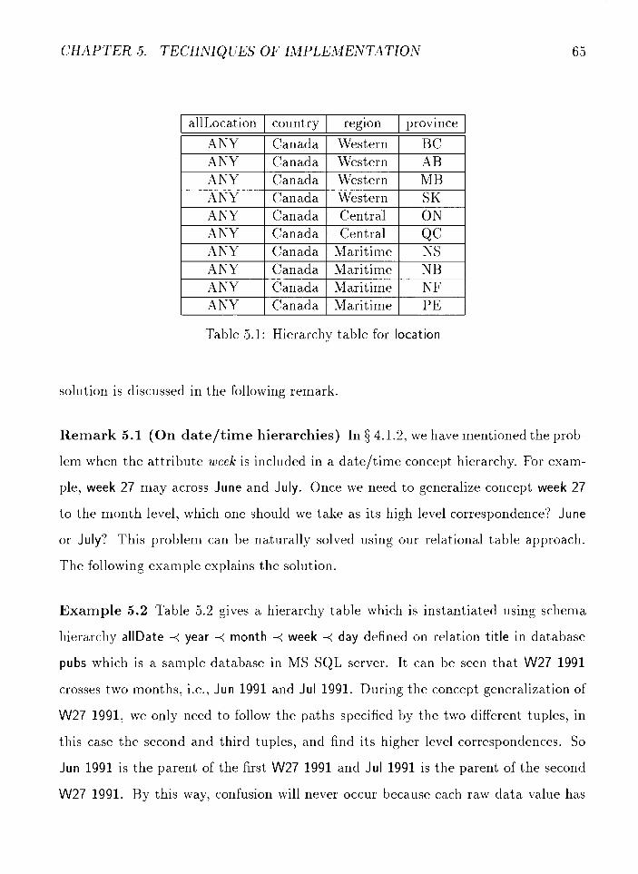
CHAPTER 5. TECHNIQUES OF IMPLEMENTATION
I allLocation I country I region I province
Table 5.1: Hierarchy table for location
solution is discussed in the following remark.
Remark 5.1 (On date/time hierarchies) In 3 4.1.2, we have mentioned the prob-
lem when the attribute week is included in a date/time concept hierarchy. For exam-
ple, week 27 may across June and July. Once we need to generalize concept week 27
to the month level, which one should we take as its high level correspondence? June
or July? This problem can be naturally solved using our relational table approach.
The following example explains the solution.
Example 5.2 Table 5.2 gives a hierarchy table which is instantiated using schema
hierarchy allDate 4 year 4 month 4 week 4 day defined on relation t i t le in database
pubs which is a sample database in MS SQL server. It can be seen that W27 1991
crosses two months, i.e., Jun 1991 and Jul 1991. During the concept generalization of
W27 1991, we only need to follow the paths specified by the two different tuples, in
this case the second and third tuples, and find its higher level correspondences. So
Jun 1991 is the parent of the first W27 1991 and Jul 1991 is the parent of the second
W27 1991. By this way, confusion will never occur because each raw data value has

CHAPTER 5. TECHNIQ UES OF IMPLEMENTATION
I I I I I ANY 1 1991 1 Jun 1991 1 W27 1991 1 Jun 30, 1991 /
allDate
ANY
I I I I 1 ANY I 1991 I Oct 1991 1 W43 1991 / Oct 21. 1991 1
year
1991
ANY ANY
I I 1 ANY 1 1994 1 Jun 1994 1 W25 1994 1 Jun 12, 1994 1 1 ANY 1 1995 1 Jun 1995 1 W23 1995 1 Jun 7, 1995 1
month
Jun 1991
Table 5.2: An date/ t ime hierarchy table
1991 1991
its unique higher level correspondence.
week
W24 1991
W27 1991 W40 1991
Jul 1991 Oct 1991
Finally, it is valuable to notice that to achieve the goal of efficient access, related
indices are created on the tables described above. The advantage of our relational
table approach for storing hierarchies is gained incorporating with the hierarchy en-
coding strategy which is presented in the next section.
day Jun 12, 1991
Jul 2, 1991 Oct 5 . 1991
5.2 Encoding of Concept Hierarchy
As addressed in the last section, concept hierarchies can be stored in relational
databases by using three kinds of tables: chHeader and chLevel and hierarchy ta-
ble. To use the hierarchies for concept generalization in data mining, however, the
above described hierarchy tables still does not fit our need. It is not feasible to retrieve
the tables to memory or put concepts directly into corresponding cube cells because
some hierarchies might be as large as or bigger than the database on which we are
executing mining tasks, and the character strings for describing those concepts could
be very long. The direct concept retrieval might only allow us to handle small size

CHAPTER 5. TECHNIQUES OF IMPLEMENTATION 6 7
data cubes, and in this case we need to spend a lot of time to process mining tasks
because of the memory page swapping. Hierarchy encoding strategy is introduced to
tackle this problem. We attempt to encode a concept hierarchy in such a way that
the partial order of the hierarchy is exactly represented by the codes so that we only
need to manipulate the codes when we process mining tasks. The access of the stored
concept hierarchy is only needed when we want to create a data cube and to display
a mining result once a mining task is fulfilled.
store
Figure 5.1 : Post-order traversal encoding of a small hierarchy.
A hierarchy encoding method is proposed in Wang and Iyer[49] according to a
post-order traversal of the hierarchy. For example, Figure 5.1 illustrates an encoded
simple hierarchy for a retail store data. The post-order traversal encoding has the
following property: for any node with label j, if the smallest label of its descendents
is i , then i < j and it has exactly ( j - i ) descendents with labels from i to ( j - 1).
Thus all the integers in the range [i, j - 11 gives the labels of all its descendents.
This encoding scheme is suitable for the drill-down operation in OLAP, especially
when cooperated with the DB2 features[6]. However, there does not appear to be any
reasonable way to extend it to the other operations or data mining functionalities.

CHAPTER 5. TECHNIQUES OF IMPLEMENTATION
5.2.1 Algorithm
A new hierarchy encoding algorithm is proposed in this subsection which can be
treated as a generic purpose encoding strategy suitable for any data mining function-
alities. The main idea is to assign each node (or concept) of a hierarchy a unique
binary code which consists of j fields, where j is the level number of the node in
this hierarchy. Once a hierarchy is encoded, we only need to retrieve the codes of
the hierarchy to the memory and realize generalization and specialization by manip-
ulating the codes. The performance analysis discussed in the next section will clearly
demonstrate the advantage of our hierarchy encoding scheme.
To describe our encoding algorithm, let us first introduce several notations.
Denote by {Pi)zl the set of all the distinct root-leaf paths in the hierarchy 3.1,
and let
Pi = (ai07 ail, - . -> ai.l-l), i = 1 , 2 ,..., m.
where aij is the j t h node which corresponds to the j t h level of the hierarchy on the
path Pi. The encoding algorithm is described as follows.
Algorithm 5.1 (Encoding of Concept Hierarchy) Assign a binary code to each
node of a concept hierarchy such that the partial order of the hierarchy is represented
by the set of codes.
Input: A concept hierarchy 3.1 from which the set of root-leaf paths {P;)z"=,s sorted
in ascending order and the maximum number of siblings, denoted by s j for each
level j = 0,1, ..., (1 - 1) is given.
Output: A set of binary codes which are assigned to the root-leaf paths of hierarchy
3.1.

CHAPTER 5. TECHNlQUES OF IMPLEMENTATION
Method: The encoding algorithm consists of the following steps:
1. Initialize the array of binary numbers (co, cl, ..., cl-I), i.e., cj := 1 (3 =
0,1, ..., (1 - I ) ) , where each binary number cj has [log,(sj + 1)J bits.
2. Assign code c = coc l...cj which is the concatenation of j binary numbers
ck, k = 0,1, .., j, to node a l j for each j = 0,1, ..., ( I - 1); set i = 2 and do
while ( i 5 m) {
for ( j = O ; j < I ; j + + ) {
if aij # a;-I j {
cj := cj + 1;
assign code c = co ... cj to node a;j;
for (k = j + 1; k < I; k + +) {
cl, := 1;
assign code c = cck to node ail,; }
j : = l - 1 ; ) )
i : = i + l ; }
To ease our discussion below, we call cj a partial code corresponding to level j in a
code cocl. . . ~ j - ~ c j c j + ~ ... eldl.
Example 5.3 Apply the above algorithm to the concept hierarchy shown in Fig-
ure 5.1, we get an encoded hierarchy demonstrated in Figure 5.2.
5.2.2 Properties
For the computational complexity of the encoding algorithm 5.1, we have the following

CHAPTER 5. TECHNIQUES OF IMPLEMENTATION
Figure 5.2: An encoded concept hierarchy.
Theorem 5.1 The computational complexity of the algorithm 5.1 is O ( l m ) , where 1
is the number of levels, and m is the number o f leaf nodes of a hierarchy.
Proof The theorem follows from the fact that we have to perform 1 operations for
each root-leaf path and there are m paths.
To explain the relationship between the partial order of a concept hierarchy and
its codes produced by algorithm 5.1, we first give a property of the codes.
Lemma 5.1 For any two nodes A and B with codes C A ~ C A ~ ... CA, and c ~ , c ~ , ... c ~ , ,
respectively, A is a child o f B if and only i f i = j + 1 and c ~ , = c ~ , for k = 0, 1, . . . j .
Proof If A is a child of B, then the code for A has one more field than of B and the
code of A is formed by concatenating a binary number to that of B, thus i = j $ 1
and CA, = CB, for k = O,l, ...j.
On the other hand, if i = j + 1 and c ~ , = c ~ , for k = 0, 1, ...j, but A is not a child
of B, we attempt to generate contradiction. We only need to consider the situation
that A and B are not at the same level, since otherwise we will have i = j which is
an obvious contradiction t o i = j + 1. Since A is not a child of B, we have the cases
of either they are on the same root-leaf path or on two different root-leaf paths. Let
us first consider the same path case. Since A is not a child of B, according to the

C H A P T E R 5. TECHNIQUES OF IMPLEMENTATION 71
algorithm, the number of fields in the code for A is at least two more or no larger
than that of B , in other words, i > j + 2 or i < j . This contradict to i = j + 1.
Now let us consider the case that A and B are on two different root-leaf paths and
2 = j + 1. In t,his ca.se7 A's parent P with code, say, cpocp, ... cp,, is at the same level
as B. P # B since A and B are on different paths, thus there must be at least one
t such that 0 5 t 5 j, cs , # cp,. Since the code for A is formed by concatenating
cp,cp, ... cp, with another binary number, we have c ~ , = cp, for k = 0, 1, ..., j, and
thus eg, # C A , , which contradicts to that CA, = C B ~ for k = O , l , ...j.
From this Lemma, it is easy to see that the code for the parent of a node at level
j with code cocl ... cj can be formed by dropping its partial code cj corresponding to
level j and get ~ ~ c ~ . . . c j - ~ . Based on this property, we only need to store the codes of
leaf nodes. The codes for other nodes can be easily obtained by simply chopping off
one of its leaf node code to certain levels.
The following theorem reveals the relationship between the partial order of a hi-
erarchy and its codes.
Theorem 5.2 Given the partial order 4 of hierarchy 'FI and the codes obtained by
applying algorithm 5.1 we have, for any pair of nodes A and B with codes c ~ , c ~ ~ ... c ~ ,
and cgocg I . . . cgj, respectively, A 4 B i f and only i f i > j and c ~ , = c ~ , for k =
0, l7 .. . j .
Proof A 4 B if and only if B is an ancestor of A. The theorem follows by repeatedly
applying Lemma 5.1. 0
According to this theorem, we can realize the manipulations of a concept hierarchy
by only using its codes. This is the base of executing concept generalization and
specialization in our data mining system.

C H A P T E R 5. TECHNIQUES OF IMPLEMENTATION
5.2.3 Remarks
In the input statement of the encoding algorithm 5.1, we posed the requirements that
the set of root-leaf paths is sorted and that the maximum number of siblings at each
level is available. These requirements can be achieved using the methods discussed in
the remarks below.
Remark 5.2 As discussed in the previous section, the content of a hierarchy is stored
in a relational table. So the requirement that the set of root-leaf paths is sorted in
the input of the above algorithm is easy to be implemented using a SQL query by
specifying an attribute list on which an order by statement is formed. This utilization
of SQL allow us to avoid coding sorting algorithms and, together with the indices
created on the hierarchy table, to obtain efficient execution. For example, assuming
that we have level names ao, a l , ..., and a / - I , and the hierarchy table is hierTable,
then the following SQL query realizes the sorting task and the result is stored in table
tempHierTa ble.
SELECT a0, al, . . . , al-I INTO t empHierTable FROM hierTable ORDER BY aO, a1, . . . , al-I ASC
Remark 5 .3 To satisfy the second requirement that the maximumnumber of siblings
sl for each level I = 0 ,1 , ..., ( I - 1) is calculated, we need to execute several SQL queries
and introduce a couple of auxiliary tables. The solution is detailed in the following
algorithm.
Algorithm 5.2 (Count Maximum Numbers of Siblings) Count the maximum
number of siblings at each level of a hierarchy based on its hierarchy table.

CHAPTER 5 . TECHNIQUES OF IMPLEMENTATION 7 3
Input . A concept hierarchy li whose hierarchy table is hierTable and level names are
ao, a l l ..., and
Output . The maximum number of siblings for each level.
Method. Execute the following SQL queries sequentially for each i = 0,1, . . . , (1 - 1).
1. SELECT aO, . . . , ai, thecount = COUNT(*)
INTO tempstatsl FROM hierTable GROUP BY aO, . . . , ai
SELECT thecount = COUNT(*) INTO tempStats2 FROM tempStats1 GROUP BY aO, . . . , ai-I
SELECT MAX (thecount) FROM tempStats2
To ease the task of calculating the maximum numbers of siblings, an alternative
is to count the number of nodes at each level by executing queries:
1. SELECT aO, . . . , ai, thecount = COUNT(*) INTO tempStats1
FROM hierTable GROUP BY aO, . . . , ai
SELECT COUNT(*)
FROM tempstatsl
If we replace the maximum numbers of siblings with the numbers of nodes, and still
denoted by s j , j = 0,1, ..., ( I - l ) , the method in the algorithm 5.1 can be executed
for hierarchy encoding without any modification. Although s j , j = 0,1, ... , ( I - 1)

CHAPTER 5 . TECHNIQUES OF IMPLEMENTATION 74
might be larger in the case of numbers of nodes, [log2(sj + I)], _I = 0,1, ..., (1 - l ) ,
are excepted to be not much larger than the corresponding numbers in the case of
maximum numbers of siblings. Hence, it is feasible to employ this simple approach in
Step 2 of algorithm 5.1.
Remark 5.4 Because each tuple in the hierarchy table represents a root-leaf path in
X, and the codes generated for the leaf nodes are actually associated with these paths
respectively, we can record these codes by adding one more attribute (column), say
code, to the hierarchy table. An index can also be created on this attribute in order
to efficiently access the codes of the hierarchy.
I alllocation 1 country I region 1 province I code /
Table 5.3: An encoded hierarchy table
ANY ANY
Example 5.4 After applying the encoding algorithm 5.1, the hierarchy table 5.1 be-
comes Table 5.3 . Where the data type for attribute code is binary. Since one byte
of binary data is expressed by a group of two characters, the values of code look like
hexadecimal data, but in fact they are in bit patterns. For example, 6A is actually
01101010.
Canada Canada
Maritime Maritime
NF PE
72 74

C H A P T E R 5 . TECHNIQUES OF IMPLEMENTATION
pName
Western Western Western Western Central Central
Maritime Maritime Maritime Maritime
I 1 Central I Canada /
cName
Western
I / Maritime I Canada I
pName
Canada
Table 5.4: Hierarchy tables for approach A
5.3 Performance Analysis and Comparison
In this section, we analyze the performance of using concept hierarchies without and
with encoding. Analytical estimates for both storage requirement and disk access
time are given for the following three approaches:
Approach A: without encoding. Use a collection of several tables for storing one
concept hierarchy in which real concepts are used as join key.
A concept hierarchy consists of several relations, each of which is a map table
from a lower level to its next higher level. For example, the hierarchy location
shown in Figure 3.1 is stored by using the two tables shown in Table 5.4.
Approach B: without encoding. Use a collection of several map tables for storing
a hierarchy in which concept identifier is used as join key.
Adopted by usual OLAP systems (see [49]), this approach is similar to approach
A, but, instead of using real concept name as join key between tables, here an
unique integer identifier is assigned to each node for the purpose of table join.

C H A P T E R 5. TECHNIQUES OF IMPLEMENTATION
Table 5.5: Hierarchy tables for approach B
1 cID I d a m e I pID 1
Again we use the hierarchy location to illustrate the idea of the approach. The
collection of the three tables in Table 5.5, which have the schema of (clD, cName,
cID
14
plD), gives the whole hierarchy.
cName
Canada
Approach C: with encoding. Use one relational table for each concept hierarchy.
This is the approach we employed in our implementation. An example is given
in Table 5.3.
Before proceeding to the comparison of storage requirement and disk access time,
we state the assumptions and notations used in the analysis below. First, for a typical
concept hierarchy, say, hiera,rchy X;, we denote by 1; its number of levels, F; its fan-out ,
n;j its number of nodes at level j and s;j its maximum nurnber of siblings at level j for
j = 0,1, . . . , (2; - 1). We assume that each concept in this hierarchy is represented by a
character string with length Ri bytes. Second, we assume that B f -tree indices have
been built on the related attributes on relational tables for storing concept hierarchies
and a node of the B+-tree just fits one page having size of B bytes in the disk storage.
Hence, if the sizes of a search key value and a pointer in a B+-tree are B bytes and

CHAPTER 5. TECHNIQUES OF IMPLEMENTATION 77
P bytes, respectively, the number of search key values in a node of the tree is ( k - 1)
and the number of pointers in a node of the tree is k, where k = [ZJ, L is the size
of the search key. Therefore, the number of levels of the B+-tree with N search keys
is /10g(~-~) N ] . It is easy to see that we need to have at most 1 + log^,-,) Nj dish
accesses to access a tuple in a relational table on which a B f -tree index is built on
the search key.
5.3.1 Storage Requirement
Storage requirement includes disk space for storing both hierarchy tables and data
cubes. Let us first consider the disk space for storing a typical hierarchy 3-C;.
For approach A, we need to use ( I ; - 1) tables. There are nij tuples for the table of
representing the relationship between level j and level ( j - 1). Since a concept is of
length R;, the size of this table is nij2R;. Thus the total size of the (1; - 1) tables is
For approach B, 1; tables are needed. There are nij tuples for the table of rep-
resenting the relationship between level j and level ( j - 1). If we assume that each
integer occupies I bytes, then each tuple of the table needs (R; + 21) bytes. So the
size for this table is (R; + 21)nij bytes. Totally, we need
1,-1 1,-1
S H ~ = C ( R ~ + 21)nii = (Ri + 21) nij (bytes) (5.2)
to store a hierarchy.
For approach C, since the maximum number of siblings at level j is s; j for j =
0,1, ..., ( I ; - I ) , we can easily figure out that the length of the code for a leaf node is
1,-1
Li = log,(sij + 1)/8 (bytes) j=O

CHAPTER 5. TECHNIQUES OF IMPLEMENTATION 78
There are n;,(r,-l) tuples in the encoded hierarchy table and each tuple is of size
(liRi + L;), thus the size of this hierarchy table is
Now, let us consider the storage requirement for a typical least generalized data
cube. Suppose there are d dimensions in the data cube, each of which is organized
as a hierarchy. We also assume that the measurements of the data cube requires m
bytes t o store in each cube cell.
Since there are totally n$l(ni,(l ,-l) + 1) cube cells in the least generalized cube,
we conclude that the storage requirements for approaches A, B and C are respectively
and
bytes, where L; is given by (5.3).
Summing up the above analysis, especially equations (5.1)-(5.7), we have the
following
Theorem 5.3 The storage requirements of both d concept hierarchies and the cor-
responding least generalized data cubes consisting of d dimensions organized as the
hierarchiesfor approaches A, B and C , denoted by SA, SB and Sc, are respectively

CHAPTER 5. TECHNIQUES OF IMPLEMENTATION 79
In the special case of n;j = F! for i = 1,2, ..., d and j = 0,1, ..., (1; - I ) , we can
simplify the above formula and have
where L; = [l + (li - 1) log2(Fi + 1)]/8.
Example 5.5 Let us consider the case that R; = R, I ; = 1, F; = F for i = 1,2 , .. , d.
And 1 = 4(bytes), m = 4(bytes). Figures 5.3, 5.4, 5.5, 5.6 and 5.7 demonstrate the
comparisons of storage requirement for the following five cases:
1. We vary the number of dimensions from which a data cube is built, and the
other parameters are fixed as R = 20, 1 = 4, F = 6. Figure 5.3 is plotted
using a linear scale for x-axis and a logarithmic scale for y-axis. As shown
in the figure, the required disk space is increased exponentially with respect to
the number of dimensions for each of these approaches. approach C needs less
space than the other two. For each different number of dimensions, the encoding
approach saves more than 80% and 36% of the space required by approaches A
and B respectively.
2. We change the number of levels of concept hierarchies and the other parameters
are fixed as d = 3, R = 20, F = 6. By the semilog plotting for the total disk

C H A P T E R 5. TECHNIQUES OF IMPLEMENTATION
0.0001
1 e-05 2 2.5 3 3.5 4 4.5 5
number of dimensions
Figure 5.3: Storage comparison for different number of dimensions.
Approach A - Approach B + Approach C +
2 2.5 3 3.5 4 4.5 5 5.5 6 number of levels
Figure 5.4: Storage comparison by varying number of levels.

C H A P T E R 5. TECHNIQUES OF IMPLEMENTATION 81
space, we can see from Figure 5.4 that, with the increase of number of levels, the
required space is also increasing exponentially for each approach. And approach
C needs the least space among the three methods. It respectively saves more
than 84% and 37% of the space needed by approach A and approach B.
3. We change the fan-out of concept hierarchies from 2 to 10 and fix the other
parameters as d = 3, R = 20, 1 = 5. Figure 5.5 shows, again, that the encoding
approach is the best among the three and it respectively saves about 84% and
38% of the space needed by approach A and approach B when the fan-out is no
larger than 8. The degree of the space savings is decreasing when the fan-out
is increasing. Notice that the number of leaf nodes of each hierarchy is also
increasing in this case.
I I - 1 I 1 I 7--
Approach A - Approach B -+ Approach C +
Figure 5.5: Storage comparison for different fan-out in hierarchies.
4. We vary the average length of character strings representing concepts from 5 to
30 and fix the other parameters as d = 3, 1 = 5, F = 6. In this case, the disk

CHAPTER 5 . TECHNIQUES OF IMPLEMENTATION
22
20
18
16
14
12
10
8
6
4
2 5 10 15 20 25 30
average length of concepts
Figure 5.6: Storage comparison for different concept lengths.
spaces needed for approaches B and C are increasing very slowly. We even cannot
detect the changes from Figure 5.6. The linear increasing nature for approach A is
obvious. The conclusion we can draw from this observation is that the changing
of the concept length has little affect to the length of code in approach C and
the spaces required for storing data cubes in the three approaches dominate
the total spaces. Again, the approach C is the best and it saves from 70% to
89% space relative to approach A when the concept length varies from 10 to 30.
Approach B is 37% better than approach A in any case.
5. The number of leaf nodes of each hierarchy is fixed as N = 5000. And cl = 3,
R = 10. Let the fan-out vary from 2 to 30 and the number of levels is calculated
using I = 1 + [logF N1. In this case the number of nodes at the last but one level
may not exactly follow the formula n;j = Fl. The formula in Theorem 5.3 is used
in the calculation. We can find from Figure 5.7 that all the three approaches are

CHAPTER 5. TECHNIQUES OF IMPLEMENTATION
Approach A +- ~ ; ^ 3 3 : C + + + 4 ~ C . ^ ; c ^ r + - 4 O ^ ^ ~
approach C +-
0 5 10 15 20 25 30 f an-out
Figure 5.7: Storage comparison the number of leaf nodes in hierarchies is fixed.
not sensitive t o the changing of fan-out and number of levels while the number
of leaf nodes are fixed, which indicates that the overall storage is dominated by
the number of leaf nodes. Again, the encoding approach (approach C) is the best
among the three methods and it is about 61% and 19% better than approaches
A and B respectively when the fan-out is greater than 2. The curve for approach
C also gives us indication of how to choose a reasonable fan-out. Apparently,
too large fan-out will make the number of levels too small, and too small fan-out
will give us too large number of levels. In the current case, fan-out around 6
give us better saving of storage.
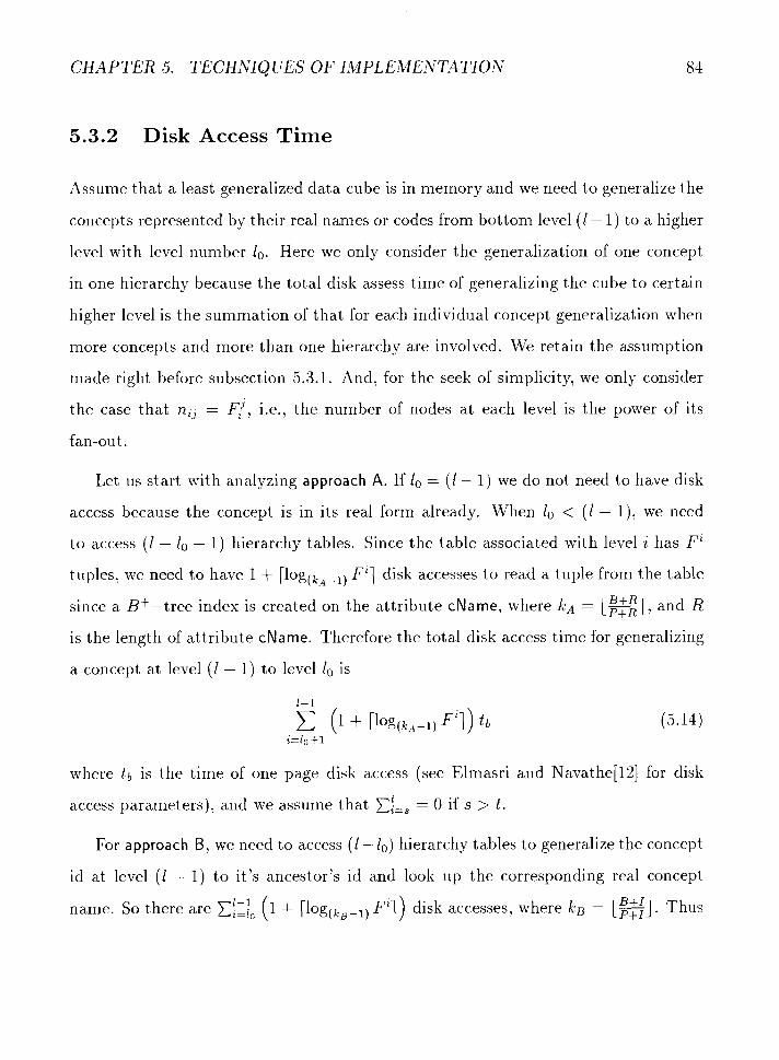
C H A P T E R 5. TECHNIQUES OF IMPLEMENTATION
5.3.2 Disk Access Time
Assume that a least generalized data cube is in memory and we need to generalize the
concepts represented by their real names or codes from bottom level ( I - 1 ) to a higher
level with level number lo. Here we only consider the generalization of one concept
in one hierarchy because the total disk assess time of generalizing the cube to certain
higher level is the summation of that for each individual concept generalization when
more concepts and more than one hierarchy are involved. We retain the assumption
made right before subsection 5.3.1. And, for the seek of simplicity, we only consider
the case that n;i = F!, i.e., the number of nodes at each level is the power of its
fan-out.
Let us start with analyzing approach A. If lo = (1 - 1) we do not need t o have disk
access because the concept is in its real form already. When lo < ( I - 1)' we need
to access ( I - lo - 1) hierarchy tables. Since the table associated with level i has Fi
tuples, we need to have 1 + [log(kA-,) F'] disk accesses to read a tuple from the table
since a B+-tree index is created on the attribute =Name, where ka = i s ] , and R
is the length of attribute cName. Therefore the total disk access time for generalizing
a concept at level (1 - 1) to level lo is
where tb is the time of one page disk access (see Elmasri and Navathe[12] for disk
access parameters), and we assume that Cf=, = 0 if s > t .
For approach B, we need to access ( I - l o ) hierarchy tables to generalize the concept
id at level ( 1 - 1) to it's ancestor's id and look up the corresponding real concept
name. So there are c/I:, (1 + [log(kB-,) ~ ' 1 ) disk accesses, where ks = [ E l . Thus

CHAPTER 5 . TECHNIQ UES OF lMPLEMENTATlON
we conclude that the total disk access time for approach B is
For approach C, to generalize a concept with a code from level ( I - 1) to level lo
we only need to chop off the code by ( I - lo - 1) fields. Disk access is need to look up
the real concept name corresponding to this generalized code in order to display the
mining result. The method of chopping off code and looking up real concept names
will be addressed in the next chapter. Again, since a B+-tree index is created on
the attribute code for the hierarchy table, we need to access disk 1 + [log(kc-l) FL1l times, where kc = [El, and L is the length of a code. Thus, the disk access time
for approach C is
Based on the above discussion, we have the following
Theorem 5.4 Th,e disk access times of generalizing a concept in hierarchy 'FI, with
number of levels 1 and fan-out F , from bottom level ( I - 1 ) to its ancestor at level lo
for approaches A, B and C are, respectively
Example 5.6 Figure 5.8 illustrates the comparison of disk access times for the three
approaches. The typical values of parameters used in plotting the graph are as follows:
B = 512(bytes), P = 5(bytes), t b = 30(msec), F = 6, R = 20, I = 4, 1 = 5. The
x-axis is the number of generalized levels, i.e., (1 - lo - 1). As shown in the figure,
the disk access time using encoded hierarchy (approach C) is constant which can also
be detected from equation (5.19). It is more important to notice that the disk access

C H A P T E R 5. TECHNIQUES OF IMPLEMENTATION
I I I I
Approach A -+
Approach B +
0 1 2 3 4 5 number of generalized levels
Figure 5.8: Comparison of disk access time for generalizing a concept.
time of approach C is much less than that of approaches A and B, except that we do not
perform any generalization and display only the result in the least generalized cube.
With the increasing of the number of generalized levels, the performance superior
of the encoding method is also increasing. For example, the encoding approach is 4
times faster than approach A or approach B when a concept is generalized from level
4 to level 1. Finally, we point out that approach B is slower that approach A because,
comparing to approach A, we need to access one more hierarchy table in using approach
B to generalize a concept to a certain level.
Based upon the comparison of storage and disk access time for the three approaches,
we can conclude that the encoding approach outperforms the two without-encoding
approaches. The encoding method gives us a way to spend less storage and obtain
more efficient processing of data mining tasks.

CHAPTER 5. TECHNIQ UES OF IMPLEMENTATION
5.4 Discussion and Summary
After discussing the relational table method of storing concept hierarchies, we focus on
study of the encoding technique in order to efficiently implement concept hierarchies
in data mining systems. The idea of assigning binary numbers to the nodes of concept
hierarchies has also been employed in other areas such as logic programming, digital
source coding and data compression. The encoding algorithm we developed here can
be natural integrated with the relational database approaches. The algorithm could
be utilized for any task of data mining when concept generalization is the base of a
data mining system. Actually, the encoding algorithm implemented in our DBMiner
system is used for data cube creation as well as for all the functional modules such
as summarizer, comparator, associator, classifier and predictor. The performance
analysis for both storage requirement and disk access time shows the superior of our
encoding approach.
We emphasize that the encoding algorithm we proposed is useful and efficient
especially for concept generalization. There may exist other encoding techniques for
other applications of concept hierarchies. We did not perform a comparison study
for those ones because there are no applications in data mining. We even did not
compare our technique with the one proposed by Wong and Iyer[49] because their
encoding technique can only be used for the drill-down operation. Further research is
needed to examine other encoding methods in artificial intelligence, data compression
and other fields in order to extend their applications to data mining.
Notice that, the CPU times of executing functional modules are not compared
here because, for any particular module, once shorter codes (compared to real concept
names) are involved in the related operations, less computational time will also be
gained.

Chapter 6
Data Mining Using Concept
Hierarchies
As one of the core parts of the DBMiner system, concept hierarchies play a central
role in processing data mining tasks. In this chapter, we will discuss the application of
concept hierarchies in mining knowledge from databases, especially, in the DBMiner
system. The system is briefly addressed in section 6.1. Following the flow of executing
a particular data mining query (or task), we will discuss why and how to expand the
query in order to correctly retrieve the so called task-relevant data in section 6.2. In
section 6.3, the issue of concept generalization is discussed. The problem of using
rule-based concept hierarchies is examined in section 6.4. In section 6.5, we consider
the issue of concept lookup which is the last step of processing a data mining task for
displaying final results. Finally, this chapter is summarized in section 6.6.

C H A P T E R 6. DATA MINING USING CONCEPT HIERARCHIES
6.1 DBMiner System
A data mining system, DBMiner, has been developed, which is the integration of
functional modules, including data mining modules, data communication module,
GUI and concept hierarchy module. Figure 6.1 illustrates the architecture of the
system. It is clear that the utilization of concept hierarchies is the base of the system.
Graphical User Interface
DB Server
Concept Hierarchy &---TL- Figure 6.1: Architecture of the DBMiner system.
Discovery modules include summarizer, comparator, associator, classifier and pre-
dictor. The application of concept hierarchies is involved in the data cube generation
and each of the above functional modules. The major applications are discussed in
the rest sections.
6.2 DMQL Query Expansion
First of all, let us consider a data mining example:
Example 6.1 Suppose that a database U NlVERSlTY has the following schema:

CHAPTER 6. DATA MINING USING CONCEPT HIERARCHIES
student(name, sno, status, major, gpa, birth-date, birth-city, birth-province)
course(cno, name, department)
grading(sn0, cno, instructor, semester, grade)
In order to discover some hidden regularities in this database, we specify the following DMQL query:
USE d a t a b a s e UNIVERSITY MINE CHARACTERISTIC RULE FROM s t u d e n t WHERE major="cs" and gpa=I13. 5-4.0" and bir th-place="CanadaW I N RELEVANCE TO gpa , b i r t h - p l a c e ANALYZE count
One may immediately find from this query that birth-place is not an attribute in table
student, and "3.5-4.0" is not a value for attribute gpa. Actually, the two dimension
gpa and birth-place appearing in the IN RELEVANCE TO statement are associated with
concept hierarchies gpa and birth-place. And "3.5-4.0" and Canada are two concepts
in the mentioned hierarchies, respectively.
To transform this query into a SQL query to retrieve task-relevant data and to
complete the mining task, we need to get the following two things done.
Expand dimensions. The dimensions involved in the "in relevance to" clause should
be expanded in order to get a SQL select statement. The attributes in the SQL
select statement must be available in database tables. In the above DMQL query,
dimension gpa is an attribute in table student, but birth-place is not. Assume that
hierarchy birt h-place has level names all-place(C), count ry(C), birt h-province(S)
and birth-city(S), where the letters C or S in the parentheses indicate the type of
the levels. The dimension birth-place is replaced with birth-province and birt h-city
which are of type S(schema). Now, the SQL select statement is
SELECT gpa , b i r th -p rov ince , b i r t h - c i t y

C H A P T E R 6. DATA MINING USING CONCEPT HIERARCHIES 9 1
Expand where clause. The higher level concepts in the where clause of DMQL
query have to be expanded so that only raw data values are involved in the
formed SQL where clause. For example, "Canada" is not a value in table student.
We use concept hierarchy birth-place, which is identical to hierarchy location
shown in Figure 3.2, to find the nearest descendents of schema type which
have level name birth-province and values of the nine provinces. Thus, after
expanding, the condition b i r t h - p l a c e = "Canada" is replaced with
b i r t h - p r o v i n c e = BC OR b i r t h - p r o v i n c e = "AB"
OR b i r th -p rov ince = "MB" OR b i r th -p rov ince = "SK"
OR b i r th -p rov ince = "ON" OR b i r th -p rov ince = "QC"
OR b i r th -p rov ince = "NS" OR b i r t h - p r o v i n c e = "NB"
OR b i r th -p rov ince = "NF" OR b i r t h - p r o v i n c e = "PEW.
Other conditions having higher level concepts can be handled similarly.
6.3 Concept Generalization
Roll-up and drill-down are two of the most useful and attractive operations in data
mining and data warehousing. These two operations are all cooperated with concept
generalization using concept hierarchies. We have considered some of the operations
in Chapter 5 for the purpose of estimating disk access time. Here are the detailed
discussions.
Intuitively, roll-up corresponds to concept ascension using concept hierarchies.
Whileas d rill-down corresponds to concept specialization, i.e. find the children or
descendents and perform related operations. In our DBMiner system, the two oper-
ations are implemented in a uniformed way, that is they are all realized by concept
generalization. Actually, a least generalized data cube is stored as a base data for all

C H A P T E R 6. DATA MINING USING CONCEPT HIERARCHIES
the operations. Once we need to roll up to a particular level of a concept hierarchy, we
generalize the data in the least generalized data cube to that level and perform related
computation. On the other hand, if we need to drill down to some level, we also use
that data cube and generalize its data to that level. Therefore, concept generalization
is core part of roll-up and drill-down.
Using the concept hierarchies which have been encoded using the method ad-
dressed in Chapter 5 , concept generalization is an easy task. Since there is a code
for each root-leaf path in a hierarchy, that is there is a code for each leaf node. The
codes of the concept hierarchy will be retrieved when we create the least generalized
data cube. Recall that our codes are structured as a concatenation of several fields or
levels, hence a simple chop off of last several fields of a code will realize the concept
generalization to a particular level.
Figure 6.2: A sample procedure of code chopping off
Example 6.2 Figure 6.2 illustrates the procedure for concept generalization, where
the related concept hierarchy is assumed to have four levels, and we want to generalize
the cid to level one. So the last two fields or levels are chopped off, and the code 29257
is changed to x9000.

CHAPTER 6. DATA MINING USING CONCEPT HIERARCHIES 93
6.4 On the Utilization of Rule-based Concept Hi-
erarchies
In the basic attribute-oriented induction (AOI), the values of attributes can always be
uniquely generalized to their ancestors at a given level of the corresponding concept
hierarchies. However, this is not the case in concept generalization using rule-based
hierarchies which are not converted to the non-rule-based ones like we did in $3.3.4.
Generalization may sometimes results in the loss of information[7], which could be
crucial in the following cases:
1. A generalization rule may depend on an attribute which has been removed;
2. A generalization rule may depend on an attribute value whose abstraction level
is too high to match the condition of the rule;
3. A rule may depend on a condition which can only be evaluated against the
initial relation.
To solve this information loss problem, a backtracking algorithm is proposed in
[7], in which a covering-tuple-id is introduced for each tuple in the prime relation.
To get a final mining result, the algorithm must go back to the original data relation
to find the corresponding tuple which is marked by it covering-tuple-id and execute
concept generalization again. This solution has the obvious drawback that we have
to access raw data every time when we need to perform concept generalization and
display the consequent results.
The conversion principle we presented in 53.3.4 can be used to solve the information
loss problem naturally. As a matter of fact, after a rule-based concept hierarchy
is transformed into its non-rule-based equivalence, we can perform any operations

CHAPTER 6. DATA MINING USING CONCEPT HIERARCHIES 94
applicable to a usual hierarchy, such as storing into relational tables and encoding.
To create a data cube, one needs to relate the attributes appeared in that rule-based
hierarchy together and pick up the corresponding code from the hierarchy table.
Once the data cube has been created, we no longer need to access the raw data
and all the other data mining functionalities can be executed normally.
6.5 Concept Lookup for Displaying Results of Data
Mining
By using concept codes we can perform computations related to a mining task until
we get the final stage of displaying mining results. Obviously, it does not make sense
to display the results such as rules or graphs using codes because they are meaningless
to users. We need to use the given codes to look up their corresponding concept names
from concept hierarchy tables by submitting SQL queries.
However, a simple look up will not solve the problem since, at most times, the
given codes are generalized ones, that is they are produced by concept chopping off as
described in 56.3. These codes usually does not exist in the encoded hierarchy tables.
A method for solving this problem is to find the original correspondences of the
given codes. Observing that a generalized code must have some fields which are of
value zero, we add those fields of value zero by 1 to construct a new code. This
newly formed code must appear in the hierarchy table by investigating the hierarchy
encoding algorithm 5.1. Concept name can be obtained by submitting a SQL query,
and retrieve a concept at a level corresponding to that of the generalized code.

CHAPTER 6. DATA MINING USING CONCEPT HIERARCHIES
Example 6.3 Using Example 6.2, we consider the concept look up for cid
By adding a 1 to each of the chopped off fields we get
which can be used to specify a SQL query such as
SELECT al, a2 FROM aHierTable WHERE code = lookupcode
where a1 and a2 are the first two level names of the concerned concept hierarchy.
Finally we can use the retrieved values for a1 or (at, a2) for displaying our mining
results. 0
6.6 Summary
The architecture of the DBMiner system is briefly introduced. Concept hierarchies
are used in the data cube construction and all the other functional modules. The
major applications of concept hierarchies, including DMQL query expansion, concept
generalization, the use of rule-based hierarchies and display of mining results, are
discussed using examples. Many other applications, including the retrieval and search
of hierarchy-related information, and the special treatment of timeldate hierarchies,
are also implemented in the DBMiner system.

Chapter 7
Conclusions and Future Work
Data mining and knowledge discovery in databases have been attracting a signifi-
cant amount of research, industry and media attention. As one of the important
background knowledge for data mining, concept hierarchy provides any data mining
methods with the ability of generalizing raw data to some abstraction level, and make
it possible to express knowledge in concise and simple terms. Concept hierarchies also
make it possible to mining knowledge at multiple levels. This thesis is focused on the
study of concept hierarchy concerning its specification, generation, implementation
and application. In this last chapter of the thesis, we give a brief summary of the
work we have done in the thesis and discuss some related topics which are important
and interesting for future research.
7.1 Summary
The efficient use of concept hierarchy in data mining is the ultimate goal of the study.
Different aspects of the concept hierarchy are investigated in the thesis, including its

CHAPTER 7. CONCLUSIONS AND FUTURE W O R K 97
properties, specification, automatic generation, implementation and application. In
particular, we consider the following as the major contributions of this thesis.
1. The terminology and properties of concept hierarchies have been discussed. A
set of basic terms and their definitions have introduced. The relationship be-
tween the set of concepts and the set of level names has indicated the flexibility
of specifying a hierarchy. The discussion on the four types of concept hierar-
chies has clarified their general properties and made it possible to apply specific
techniques to different types of hierarchies.
2. The automatic generation of concept hierarchies has been studied. The algo-
rithm designed for detecting a partial order on a set of nominal attributes is a
useful guide for users to defining their hierarchies. The two algorithms proposed
for automatic generation of numerical hierarchies and the performance analysis
have provided us novel tools of handling the concept generalization of numerical
attributes. The introduction of the variance quality in the partitioning cluster-
ing method has resulted in a better similarity measure for a group of objects.
Due to the popularity of numerical attributes in databases, the automatic gen-
eration of numerical hierarchies is desirable for any data mining systems.
3. The strategy for the implementation of concept hierarchies has been investi-
gated. The encoding technique of concept hierarchies has been presented. The
analysis on the storage requirement and disk access time has ensured the effi-
ciency and effectiveness of the application of concept hierarchies in data mining
systems.

CHAPTER 7. CONCLUSIONS AND FUTURE WORK
7.2 Future Work
There are still many interesting problems which are worth continuing research, some
of which are discussed as follows.
(1) How t o specify fan-out in the automatic generation o f a numerical hierarchy?
In the applications, we can display the histogram of an attribute on which a
hierarchy is to be built, and decide the value of the fan-out based on the number of
modes in the histogram. However, if this number is too large or the histogram is too
mess for us to find this number, we should have a method to make reasonably good
decision.
(2) How t o measure the qualities o f hierarchies generated by different algorithms?
There are quality measures for clustering methods. However they cannot be ap-
plied directly to measure the qualities of hierarchies. In Chapter 4, we basically
compare the qualities of hierarchies using our observation on the given histogram. It
might be difficult to judge their qualities when the given histogram is very compli-
cated.
Figure 7.1: A concept hierarchy for attribute age.
As we mentioned in Chapter 2, [21] defined the complexityof a concept hierarchy in
terms of its number of interior nodes, and the depth and height of each of these interior

CHAPTER 7. CONCLUSIONS AND FUTURE W O R K 99
nodes. This complexity is then used to measure the interestingness of discovered
rules. It seems that the quality of a concept hierarchy could be measured also by this
complexity because more interesting a rule is, higher quality the concept hierarchy
is. However, the situation is not that simple. For example, we have two concept
hierarchies as shown in Figures 7.1 and 7.2.
Figure 7.2: Another concept hierarchy for attribute age.
count
80
60
40
20
0 32 48 64 80 96 112 age
Figure 7.3: A histogram for attribute age.
Each of them is constructed by using the input histogram as shown in Figure 7.3.

C'HAPTER 7. CONCLUSIONS A N D F l
If we use the measure defined in [21]
JTURE WORK 100
, we find that the second concept hierar-
chy (Figure 7.2) has a higher quality than that of the first hierarchy (Figure 7.1).
Nevertheless, only the first hierarchy correctly describes the hidden structure of the
attribute on which the histogram is produced. Therefore, one can make sure that
knowledge rules discovered using the second hierarchy are definitely worse than those
using the first hierarchy. How to measure the quality of a concept hierarchy is still
an open problem.
(3) How t o handle complex rule-based concept hierarchies?
A deductive generalization rule has the form: A(x) A B ( x ) -+ C(x), which means
that, for a tuple x, concept A can be generalized to concept C if condition B is satisfied
by x. The condition B ( x ) can be a simple predicate or a very complex logic formula
involving different attributes and relations. The technique used in Chapter 3 can
only deal with simple predicate cases. Further researches are needed on implementing
complex rule-based concept hierarchies.

Bibliography
[I] A. A. Afifi and V. Clark. Computer-aided multivariate analysis. 3rd edition,
Chapman and Hall, NY, 1996.
[2] R. Agrawal, T. Imielinski and A. Swami. Mining association rules between sets
of items in large databases. In Proc. of the ACM SIGMOD conf. on Management
of Data, Washington, D.C., 207-216, 1993.
[3] R. Agrawal and R. Srikant. Fast algorithms for mining association rules. In Proc.
1994 Int. Conf. Very Large Data Bases, Santiago, Chile, 487-499, 1994
[4] H. Ait-Kaci, R. Boyer, P. Lincoln and R. Nasr. Efficient implementation of lattice
operations. ACM Transactions on Programming Languages, 11(1):115-146, 1989.
[5] C. Brew. Systemic classification and its efficiency. Computational Linguistics,
17(4):375-408, 1991.
[6] D. Chamberlin. Using the new DB2: IBM's object-relational database system.
Morgan Kaufmann, 1996.
[7] D. W. Cheung, A. W. Fu and J. Han. Knowledge discovery in databases: a rule-
based attribute-oriented approach. In Proc. 1994 Int. Symp. on Methodologies
for Intelligent Systems (ISMIS'94), Charlotte, NC, 164-173, 1994.

BIBLIOGRAPHY 102
[8] M. J . Corey and M. Abbey. Oracle data warehousing. Osborne McGraw-Hill:
Oracle Press, CA, 1997.
[9] V. Dahl. On database systems development through logic. ACM Transactions on
Database Systems, 7(1), 1982.
[lo] V. Dahl. Incomplete types for logic databases. Applied Math. Letters, 4(3):25-28,
1991.
[ll] DSSArchitect. Microstrategy Incorporated, VA, 1997.
[12] R. Elmasri and S. B. Navathe. Fundamentals of database systems. The Ben-
jamin/Cummings Publishing Company Inc., 1989.
[13] B. S. Everitt. Cluster analysis. Edward Arnold, 1993.
[14] A. Fall. Reasoning with taxonomies. Ph.D Thesis, School of Computing Science,
Simon Fraser University, 1996.
[15] D. Fisher. Improving inference through conceptual clustering. In Proc. 1987
A A A I Conf., Seattle, Washington, 461-465, 1987.
[16] L. Fisher and J. W. Van Ness. Admissible clustering procedures. Bipmetrika, 58,
91-104, 1971.
[17] W. J. Frawley, G. Piateetsky-Shapiro and C. J.Matheus. Knowledge discovery
in databases: An overview. In G. Piatetsky-Shapiro and W. J . Frawley, eds.
Knowledge Discovery in Databases, 1-27, AAAI/MIT Press, 1991.
[IS] M. Genesereth and N. Nilsson. Logical foundations of artificial intelligence. Mor-
gan Kaufmann. San Francisco, CA, 1987.

BIBLIOGRAPHY 103
[19] A. D. Gordon. Classification: Methods for the Exploratory Analysis and Multi-
variate. Chapman and Hall, 1981.
[20] R. P. Grimaldi. Discrete and combinatorial mathematics: An applied introduc-
tion. Addison-Wesley Publishing Company, 1994.
[21] H. J. Hamilton and D. R. Fudger. Estimating DBLearn's potential for knowledge
discovery in databases. Computational Intelligence, 11 (2), 280-296, 1995.
[22] J. Han. Mining knowledge at multiple concept levels. In Proc. 4th Int. Conf.
on Information and Knowledge Management (CIKM'95), Baltimore, Maryland,
19-24, 1995.
[23] J. Han. Conference Tutorial Notes: Integration of data mining and data ware-
housing technologies. 1997 Int71 Conf. on Data Engineering (ICDE'g?'), Birm-
ingham, England, 1997.
[24] J. Han, Y. Cai and N. Cercone. Data-driven discovery of quantitative rules in
relational databases. IEEE Tran. on Knowledge and Data Engineering, 5(1), 29-
40, 1993.
[25] J. Han and Y. Fu. Dynamic generation and refinement of concept hierarchies for
knowledge discovery in databases. In Proc. AAA1794 Workshop on Knowledge
Discovery in Databases(KDD794), Seattle, WA, 157-168, 1994.
[26] J. Han and Y. Fu. Discovery of multiple-level association rules from large
databases. In Proc. 1995 Int. Conf. Very Large Data Bases (VLDB795), Zurich,
Switzerland, 420-431, 1995.
[27] J. Han and Y. Fu. Exploration of the power of attribute-oriented induction in
da ta mining. In U. Fayyad, G. Piatetsky-Shapiro, P. Smyth and R. Uthurusamy,

BIBLIOGRAPHY 104
editors, Advances in I{nowledge Discovery and Data Mining, AAAI/MIT Press,
399-421, 1996.
[28] J . Han, Y. Fu, K. Koperski, W. Wang and 0. Zaiane. DMQL: A data mining
query language for relational databases. 1996 SIGMOD '96 Workshop on Re-
search Issues on Data Mining and Knowledge Discovery (DMKD796), Montreal,
Canada, 27-34, June 1996.
[29] V. Harinarayan, A. Rajaraman and J. D. Ullman. Implementing data cubes ef-
ficiently. Proc. 1996 ACM-SIGMOD Int. Conf. Management of Data, 205-216,
Montreal, Canada, June 1996.
[30] J. Hong and C. Mao. Incremental discovery of rules and structure by hierar-
chical and parallel clustering. In G.Piatetsky-Shapiro and W.J.Frawley, editors,
Icnowledge Discovery in Databases, 449-462, AAAI/MIT press, 1991.
[31] M. Kamber, L. Winstone, W. Gong, S. Cheng and J . Han. Generalization and
Decision Tree Induction: Efficient Classification in Data Mining. In Proc. of
1997 Int'l Workshop on Research Issues on Data Engineering (RIDE'S?'), Birm-
ingham, England, 111-120, 1997.
[32] N. Katayama and S. Satoh. The SR-tree: an index structure for high-dimensional
nearest neighbor queries. In SIGMOD797, AZ, USA, 369-380, 1997.
1331 K. A. Kaufman and R. S. Michalski. A method for reasoning with structured and
continuous attributes in the INLEN-2 multistrategy knowledge discovery system.
In Proc. The Second Int. Conf. on Knowledge Discovery & Data Mining, 232-237,
1996.
[34] L. Kaufman and P. J. Rousseeuw. Finding groups in data: an introduction to
cluster analysis. John Wiley & Sons, 1990.

BIBLIOGRAPHY 105
[35] D. Keim, H. Kriegel and T. Seidl. Supporting data mining of large databases by
visual feedback queries. In Proc. 10th Int. Conf. on Data Engineering, 302-313,
Houston, TX, Feb. 1994.
[36] R. Kerber. ChiMerge: Discretization of numeric attribute. In Proc. Tenth Na-
tional Conf. on Artificial Intelligence (AAAI-92), San Jose, CA, 123-127, 1992.
[37] J. Lebbe and R. Vignes. Optimal hierarchical clustering with order constraint. In
Ordinal and Symbolic Data Analysis, E.Diday, Y.Lechevallier and O.Opitz, eds.,
Springer-Verlag, 265-276, 1996.
[38] C. Mellish. The description identification problem. Artificial Intelligence,
52(2):151-167, 1991.
[39] R. S. Michalski. Inductive learning as rule-guided generalization and conceptual
simplification of symbolic description: unifying principles and a methodology.
Workshop on Current Developments in Machine Learning, Carnegie Mellon Uni-
versity, Pittsburgh, PA, 1980.
[40] R. S. Michalski and R. Stepp. Automated construction of classifications: Con-
ceptual clustering versus numerical taxonomy. lEEE Trans. Pattern Analysis and
Machine Intelligence, 5:396-410, 1983.
[41] R. Missaoui and R. Godin. An incremental concept formation approach for learn-
ing from databases. In V.S.Alagar, L.V.S.Lakshmanan and F.Sadri, editors, For-
mal Methods in Databases and Software Engineering, Springer-Verlag, 39-53,
1993.
[42] Powerplay: Packaging information with transformer. Cognos Incorporated, 1996.
[43] H. C. Romesburg. Cluster analysis for researchers Krieger Publishing Company,
Malabar, Florida, 1990.

BIBLIOGRAPHY 106
[44] S. J. Russell. Tree-structured bias. In Proc. 1988 AAAI Conf., Minneapolis, MN,
641-645, 1988.
[45] R. R. Sikal and P. H. A. Sneath. Principles of numerical taxonomy. W.H.Freeman
and Co., London, 1963.
[46] R. Srikant and R. Agrawal. Mining generalized association rules. In Proc. 1995
Int. Conf. Very Large Data Bases, Zurich, Switzerland, 407-419, 1995.
[47] G. Stumme. Exploration tools in formal concept analysis. In Ordinal and symbolic
data analysis, E. Diday, Y. Lechevallier and 0. Opitz (Eds.), 31-44, 1995.
[48] P. Valtchew and J. Euzenat. Classification of concepts through products of con-
cepts and abstract data types. In Ordinal and symbolic data analysis, E. Diday,
Y. Lechevallier and 0. Opitz (Eds.), 3-12, 1995.
1491 M. Wang and B. Iyer. Efficient roll-up and drill-down analysis in relational
database. In 1997 SIGMOD Workshop on Research Issues on Data Mining and
Knowledge Discovery, 39-43, 1997
[50] R. Wille. Concept lattices and conceptual knowledge systems. Computer &' Math-
ematics with Applications, 23, 493-515, 1992.